Noname manuscript No.(will be inserted by the editor)

Mixed deterministic and probabilistic networks

Robert Mateescu · Rina Dechter

Received: date / Accepted: date

Abstract The paper introducesmixed networks, a new graphical model framework for ex-pressing and reasoning with probabilistic and deterministic information. The motivation todevelop mixed networks stems from the desire to fully exploit the deterministic informa-tion (constraints) that is often present in graphical models. Several concepts and algorithmsspecific to belief networks and constraint networks are combined, achieving computationalefficiency, semantic coherence and user-interface convenience. We define the semantics andgraphical representation of mixed networks, and discuss the two main types of algorithmsfor processing them: inference-based and search-based. A preliminary experimental evalua-tion shows the benefits of the new model.

1 Introduction

Modeling real-life decision problems requires the specification of and reasoning with prob-abilistic and deterministic information. The primary approach developed in artificial intel-ligence for representing and reasoning with partial information under conditions of uncer-tainty is Bayesian networks. They allow expressing information such as “if a person has flu,he is likely to have fever.” Constraint networks and propositional theories are the most ba-sic frameworks for representing and reasoning about deterministic information. Constraintsoften express resource conflicts frequently appearing in scheduling and planning applica-tions, precedence relationships (e.g., “job 1 must follow job 2”) and definitional information(e.g., “a block is clear iff there is no other block on top of it”). Most often the feasibilityof an action is expressed using a deterministic rule betweenthe pre-conditions (constraints)and post-conditions that must hold before and after executing an action (e.g., STRIPS forclassical planning).

R. MateescuElectrical Engineering Department, California Institute of Technology, Pasadena, CA 91125E-mail: mateescu@paradise.caltech.edu

R. DechterSchool of Information and Computer Sciences, University of California Irvine, Irvine, CA 92697E-mail: dechter@ics.uci.edu

2

The two communities of probabilistic networks and constraint networks matured in par-allel with only minor interaction. Nevertheless some of thealgorithms and reasoning princi-ples that emerged within both frameworks, especially thosethat are graph-based, are quiterelated. Both frameworks can be viewed as graphical models,a popular paradigm for knowl-edge representation in general.

Markov random fields (MRF) are another type of graphical model commonly used instatistical machine learning to describe joint probability distributions concisely. Their keyproperty is that the graph is undirected, leading to isotropic or symmetric behavior. This isalso the key difference compared to Bayesian networks, where a directed arc carries causalinformation. While the potential functions of an MRF are often assumed to be strictly posi-tive, and are therefore not meant to handle deterministic relationships they can be easily ex-tended to incorporate deterministic potentials with no need of any modification. Our choicehowever is the Bayesian network due to its appeal in semanticclarity and its representationof causal and directional information. In fact, our mixed networks can be viewed not onlyas a hybrid between probabilistic and deterministic information but also as a framework thatpermits causal information as well as symmetrical constraints.

Researchers within the logic-based and constraint communities have recognized forsome time the need for augmenting deterministic languages with uncertainty information,leading to a variety of concepts and approaches such as non-monotonic reasoning, prob-abilistic constraint networks and fuzzy constraint networks. The belief networks commu-nity started more recently to look into mixed representation [Poole(1993), Ngo and Had-dawy(1997), Koller and Pfeffer(1998), Dechter and Larkin(2001)] perhaps because it is pos-sible, in principle, to capture constraint information within belief networks [Pearl(1988)].

In principle, constraints can be embedded within belief networks by modeling each con-straint as a Conditional Probability Table (CPT). One approach is to add a new variablefor each constraint that is perceived as itseffect(child node) in the corresponding causalrelationship and then to clamp its value totrue [Pearl(1988), Cooper(1990)]. While this ap-proach is semantically coherent and complies with the acyclic graph restriction of beliefnetworks, it adds a substantial number of new variables, thus cluttering the structure of theproblem. An alternative approach is to designate one of the arguments of the constraint asa child node (namely, as its effect). This approach, although natural for functions (the argu-ments are the causes or parents and the function variable is the child node), is quite contrivedfor general relations (e.g.,x+6 6= y). Such constraints may lead to cycles, which are disal-lowed in belief networks. Furthermore, if a variable is a child node of two different CPTs(one may be deterministic and one probabilistic) the beliefnetwork definition requires thatthey be combined into a single CPT.

The main shortcoming, however, of any of the above integrations is computational.Constraints have special properties that render them computationally attractive. When con-straints are disguised as probabilistic relationships, their computational benefits may be hardto exploit. In particular, the power of constraint inference and constraint propagation maynot be brought to bear.

Therefore, we propose a framework that combines deterministic and probabilistic net-works, calledmixed network. The identity of the respective relationships, as constraints orprobabilities, will be maintained explicitly, so that their respective computational power andsemantic differences can be vivid and easy to exploit. The mixed network approach allowstwo distinct representations: causal relationships that are directional and normally quanti-fied by CPTs and symmetrical deterministic constraints. Theproposed scheme’s value is inproviding: 1) semantic coherence; 2) user-interface convenience (the user can relate betterto these two pieces of information if they are distinct); andmost importantly, 3) computa-

3

tional efficiency. The results presented in this paper are based on the work in [Dechter andMateescu(2004), Dechter and Larkin(2001), Larkin and Dechter(2003)].

The paper is organized as follows: section 2 provides background definitions and con-cepts for graphical models; section 3 presents the framework of mixed networks, providesmotivating examples and extends the notions of conditionalindependence to the mixedgraphs; section 4 contains a review of inference and search algorithms for graphical mod-els; section 5 describes inference-based algorithms for mixed networks, based on BucketElimination; section 6 describes search-based algorithmsfor mixed networks, based onAND/OR search spaces for graphical models; section 7 contains the experimental evalu-ation of inference-based and AND/OR search-based algorithms; section 8 describes relatedwork and section 9 concludes.

2 Preliminaries and Background

Notations. A reasoning problem is defined in terms of a set of variables taking valueson finite domains and a set of functions defined over these variables. We denote vari-ables or subsets of variables by uppercase letters (e.g.,X,Y, . . .) and values of variablesby lower case letters (e.g.,x,y, . . .). Sets are usually denoted by bold letters, for exampleX = {X1, . . . ,Xn} is a set of variables. An assignment (X1 = x1, . . . ,Xn = xn) can be abbre-viated as ¯x = (〈X1,x1〉, . . . , 〈Xn,xn〉) or x = (x1, . . . ,xn). For a subset of variablesY, DYdenotes the Cartesian product of the domains of variables inY. The projection of an assign-mentx= (x1, . . . ,xn) over a subsetY is denoted byxY or x[Y]. We will also denote byY = y(or y for short) the assignment of values to variables inY from their respective domains. Wedenote functions by lettersf , g, h etc.

Graphical models.A graphical modelM is a 3-tuple,M = 〈X,D,F〉, where: X ={X1, . . . ,Xn} is a finite set of variables;D = {D1, . . . ,Dn} is the set of their respective finitedomains of values;F = { f1, . . . , fr} is a set of non-negative real-valued discrete functions,each defined over a subset of variablesSi ⊆X, called its scope, and denoted byscope( fi). Agraphical model typically has an associated combination operator1 ⊗, (e.g.,⊗ ∈ {∏,∑,1}(product, sum, join)). The graphical model represents the combination of all its functions:⊗r

i=1 fi . A graphical model has an associated primal graph that captures the structural infor-mation of the model:

Definition 1 (primal graph) Theprimal graphof a graphical model is an undirected graphthat has variables as its vertices and an edge connects any two variables that appear in thescope of the same function. We denote the primal graph byG = (X,E), whereX is the setof variables andE is the set of edges.

Belief networks.A belief network is a graphical modelB = 〈X,D,G,P〉, whereG = (X,E)is a directed acyclic graph over the variablesX. The functionsP = {Pi} are conditionalprobability tablesPi = {P(Xi | pai)}, wherepai = scope(Pi) \ {Xi} is the set ofparentsofXi in G. The primal graph of a belief network obeys the regular definition, and it can alsobe obtained as themoral graphof G, by connecting all the nodes in everypai and thenremoving direction from all the edges. When the entries of the CPTs are “0” or “1” only,they are calleddeterministic or functional CPTs. The scope ofPi is also called thefamilyofXi (it includesXi and its parents).

1 The combination operator can also be defined axiomatically [Shenoy(1992)].

4

A

F

B C

D

G

Season

Sprinkler Rain

Watering Wetness

Slippery

(a) Directed acyclic graph

A

F

B C

D

G

(b) Moral graph

Fig. 1 Belief network

A belief network represents a probability distribution over X having the product formPB(x) = P(x1, ....,xn) = Πn

i=1P(xi | xpai ). An evidence sete is an instantiated subset of vari-ables. The primary query over belief networks is to find the posterior probability of eachsingle variable given some evidencee, namely to computeP(Xi |e). Another important queryis finding themost probable explanation(MPE), namely, finding a complete assignment toall the variables having maximum probability given the evidence. A generalization of theMPE query ismaximum a posteriori hypothesis(MAP), which requires finding the mostlikely assignment to asubsetof hypothesis variables given the evidence.

Definition 2 (ancestral graph)Given a directed graphG, the ancestral graph relative to asubset of nodesY is the undirected graph obtained by taking the subgraph ofG that containsY and all their non-descendants, and then moralizing the graph.

Example 1Figure 1(a) gives an example of a belief network over 6 variables, and Figure1(b) shows its moral graph . The example expresses the causalrelationship between variables“Season” (A), “The configuration of an automatic sprinkler system” (B), “The amount ofexpected rain” (C), “The amount of necessary manual watering” (D), “How wet is the pave-ment” (F) and “Is the pavement slippery” (G). The belief network expresses the probabilitydistributionP(A,B,C,D,F,G) = P(A) ·P(B|A) ·P(C|A) ·P(D|B,A) ·P(F|C,B) ·P(G|F).

Constraint networks.A constraint network is a graphical modelR = 〈X,D,C〉. The func-tions are constraintsC = {C1, ...,Ct}. Each constraint is a pairCi = (Si ,Ri), whereSi ⊆ X isthe scope of the relationRi . The relationRi denotes the allowed combination of values. Theprimary query over constraint networks is to determine if there exists a solution, namely,an assignment to all the variables that satisfies all the constraints, and if so, to find one. Aconstraint network represents the set of all its solutions.We sometimes denote the set ofsolutions of a constraint networkR by ϕ(R).

Example 2Figure 2(a) shows a graph coloring problem that can be modeled as a constraintnetwork. Given a map of regions, the problem is to color each region by one of the given col-ors{red, green, blue}, such that neighboring regions have different colors. The variables ofthe problem are the regions, and each one has the domain{red, green, blue}. The constraintsare the relation“different” between neighboring regions. Figure 2(b) shows the constraintgraph, and a solution (A=red, B=blue, C=green, D=green, E=blue, F=blue, G=red) is givenin Figure 2(a).

5

C

A

B

D

E

F

G

(a) Graph coloring problem

A

BD

CG

F

E

(b) Constraint graph

Fig. 2 Constraint network

Propositional theories.Propositional theories are special cases of constraint networks inwhich propositional variables which take only two values{true, f alse} or {1,0}, are de-noted by uppercase lettersP,Q,R. Propositionalliterals (i.e., P,¬P) stand forP = true orP = f alse, and disjunctions of literals, orclauses, are denoted byα,β etc. For instance,α = (P∨Q∨R) is a clause. Aunit clauseis a clause that contains only one literal. Theresolutionoperation over two clauses(α ∨Q) and (β ∨¬Q) results in a clause(α ∨ β ),thus eliminatingQ. A formula ϕ in conjunctive normal form (CNF) is a set of clausesϕ = {α1, . . . ,αt} that denotes their conjunction. The set ofmodelsor solutionsof a for-mula ϕ, denoted bym(ϕ), is the set of all truth assignments to all its symbols that donotviolate any clause.

3 Mixing Probabilities with Constraints

As shown in the previous section, graphical models can accommodate both probabilisticand deterministic information. Probabilistic information typically associates a strictly posi-tive number with an assignment of variables, quantifying our expectation that the assignmentmay be realized. The deterministic information has a different semantics, annotating assign-ments with binary values, eithervalid or invalid. The mixed network allows probabilisticinformation expressed as a belief network and a set of constraints to co-exist side by sideand interact by giving them a coherent umbrella meaning.

3.1 Defining the Mixed Network

We give here the formal definition of the central concept ofmixed networks, and discuss itsrelationship with the auxiliary network that hides the deterministic information through zeroprobability assignments.

Definition 3 (mixed networks)Given a belief networkB = 〈X,D,G,P〉 that expresses thejoint probability PB and given a constraint networkR = 〈X,D,C〉 that expresses a set ofsolutionsρ(R) (or simply ρ), a mixed network based onB andR denotedM(B,R) =〈X,D,G,P,C〉 is created from the respective components of the constraintnetwork and thebelief network as follows. The variablesX and their domains are shared, (we could allownon-common variables and take the union), and the relationships include the CPTs inP and

6

the constraints inC. The mixed network expresses the conditional probabilityPM (X):

PM (x) =

{

PB(x | x∈ ρ), i f x∈ ρ0, otherwise.

Clearly,PB(x | x∈ ρ) = PB(x)PB(x∈ρ) . By definition,PM (x) = ∏n

i=1 P(xi | xpai ) whenx∈ ρ, and

PM (x) = 0 whenx /∈ ρ. When clarity is not compromised, we will abbreviate〈X,D,G,P,C〉by 〈X,D,P,C〉 or 〈X,P,C〉.

The auxiliary network.The deterministic information can be hidden through assignmentshaving zero probability [Pearl(1988)]. We now define the belief network that expresses con-straints as pure CPTs.

Definition 4 (auxiliary network) Given a mixed networkM(B,R), we define the auxiliarynetworkS(B,R) to be a belief network constructed by augmentingB with a set of auxiliaryvariables defined as follows. For every constraintCi = (Si ,Ri) in R, we add the auxiliaryvariableAi that has a domain of 2 values, “0” and “1”. We also add a CPT overAi whoseparent variables are the setSi , defined by:

P(Ai = 1 | t) =

{

1, i f t ∈ Ri

0, otherwise.

S(B,R) is a belief network that expresses a probability distribution PS. It is easy to see that:

Proposition 1 Given a mixed networkM(B,R) and its associated auxiliary network S=S(B,R) then:∀x PM (x) = PS(x | A1 = 1, ...,At = 1).

3.2 Queries over Mixed Networks

Belief updating, MPE and MAP queries can be extended to mixednetworks straight-forwardly. They are well defined relative to the mixed probability distribution PM . SincePM is not well defined for inconsistent constraint networks, wealways assume that the con-straint network portion is consistent, namely it expressesa non-empty set of solutions. Anadditional relevant query over a mixed network is to find the probability of a consistent tuplerelative toB, namely determiningPB(x∈ ρ(R)). It is calledCNF Probability Evaluationor Constraint Probability Evaluation (CPE). Note that the notion of evidence is a specialtype of constraint. We will elaborate on this next.

The problem of evaluating the probability of CNF queries over belief networks has var-ious applications. One application is to network reliability described as follows. Given acommunication graph with a source and a destination, one seeks to diagnose the failure ofcommunication. Since several paths may be available, the reason for failure can be describedby a CNF formula. Failure means that for all paths (conjunctions) there is a link on that path(disjunction) that fails. Given a probabilistic fault model of the network, the task is to assessthe probability of a failure [Portinale and Bobbio(1999)].

Definition 5 (CPE) Given a mixed networkM(B,R), where the belief network is definedover variablesX = {X1, ...,Xn} and the constraint portion is a either a set of constraintsR or a CNF formula (R = ϕ) over a set of subsetsQ = {Q1, ...Qr}, whereQi ⊆ X, theconstraint(respectivelyCNF) probability evaluation (CPE) taskis to find the probabilityPB(x∈ ρ(R)), respectivelyPB(x∈m(ϕ)), wherem(ϕ) are the models (solutions ofϕ).

7

4255386 46454084210626

secure keys modify table thread disabled caret clicked handle selection

browser file worker reopening editor prevent disabling properties message

hangs resource field menu value closing read-only restart text disappear

started service background switching freeze machines editable listenercomponent

≠ ≠

≠

Fig. 3 Two-layer network with root not-equal constraints (Java Bugs)

Belief assessment conditioned on a constraint network or ona CNF expressionis thetask of assessingPB(X|ϕ) for every variableX. SinceP(X|ϕ) = α ·P(X∧ϕ) whereα is anormalizing constant relative toX, computingPB(X|ϕ) reduces to a CPE task overB forthe query((X = x)∧ϕ), for everyx. More generally,P(ϕ|ψ) = αϕ ·P(ϕ ∧ψ) whereαϕ isa normalization constant relative to all the models ofϕ.

3.3 Examples of Mixed Networks

We describe now a few examples that can serve as motivation tocombine probabilities withconstraints in an efficient way. The first type of examples arereal-life domains involvingboth type of information whereas some can conveniently be expressed using probabilisticfunctions and others as constraints. One such area emerged often in multi-agent environ-ments. The second source comes from the need to process deterministic queries over a beliefnetwork, or accommodating disjunctive complex evidence which can be phrased as a propo-sitional CNF sentence or as a constraint formula. As a third case, a pure belief network mayinvolve deterministic functional CPTs. Those do not present semantical issues but can stillbe exploited computationally.

Java bugs.Consider the classical naive-Bayes model or, more generally, a two-layer net-work. Often the root nodes in the first layer are desired to be mutually exclusive, a propertythat can be enforced byall-different constraints. For example, consider a bug diagnosticssystem for a software application such as Java Virtual Machine that contains numerous bugdescriptions. When the user performs a search for the relevant bug reports, the system out-puts a list of bugs, in decreasing likelihood of it being the culprit of the problem. We canmodel the relationship between each bug identity and the keywords that are likely to triggerthis bug as a parent-child relationship of a two-layer belief network, where the bug identitiesare the root nodes and all the key words that may appear in eachbug description are the childnodes. Each bug has a directed edge to each relevant keyword (See Figure 3). In practice,it is common to assume that a problem is caused by only one bug and thus, the bugs on thelist are mutually exclusive. We may want to express this factusing a not-equal relationshipbetween all (or some of) the root nodes. We could have taken care of this by putting all thebugs in one node. However, this would cause a huge inconvenience, having to express the

8

Past-Grade(S1,C4) Past-Grade(S1,C5)

Type(S1) Professor(C1) Enrolled(S1,C1) Professor(C2) Enrolled(S1,C2) Professor(C3) Enrolled(S1,C3)

Grade(S1,C1) Grade(S1,C2) Grade(S1,C3)

Class-Size(C1) Class-Size(C2) Class-Size(C3)Number-of-classes(S1)

Fig. 4 Mixed network for class scheduling

conditional probability of each key word given each bug, even when it is not relevant. Javabug database contains thousands of bugs. It is hardly sensible to define a conditional proba-bility table of that size. Therefore, in the mixed network framework we can simply add onenot-equal constraint over all the root variables.

Class scheduling.Another source of examples is reasoning about the behavior of an agent.Consider the problem of scheduling classes for students. A relevant knowledge base can bebuilt from the point of view of a student, of the administration or of the faculty. Perhaps, thesame knowledge base can serve these multiple reasoning perspectives. The administration(e.g., the chair) tries to schedule the classes so as to meet the various requirements of thestudents (allow enough classes in each quarter for each concentration), while faculty maywant to teach their classes in a particular quarter to maximize (or minimize) the attendanceor to better allocate their research vs. teaching time throughout the academic year.

In Figure 4 we demonstrate a scenario with 3 classes and 1 student. The variables cor-responding to the studentSi can be repeated to model all the students, but we keep thefigure simple. The dotted lines indicate deterministic relationships, and the solid arrowsindicate probabilistic links. The variables are:Enrolled(Si ,Cj) meaning “studentSi takescourseCj ”; Grade(Si ,Cj) denoting the grade (performance) of studentSi in courseCj ; Past-Grade(Si ,Cj) is the past performance (grade) of studentSi in Cj (if the class was taken); thevariablePro f essor(Cj) denotes the professor who teaches the classCj in the current quar-ter, andType(Si) stands for a collection of variables denoting studentSi ’s characteristics(his strengths, goals and inclinations, time in the programetc.). If we have a restrictionon the number of students that can take a class, we can impose aunary constraint (Class-Size(Ci) ≤ 10). For each student and for each class, we have a CPT forGrade(Si ,Cj) withthe parent nodesEnrolled(Si ,Cj), Pro f essor(Cj) andType(Si). We then have constraintsbetween various classes such asEnrolled(Si ,C1) andEnrolled(Si ,C2) indicating that bothcannot be taken together due to scheduling conflicts. We can also have all-different con-straints between pairs ofPro f essor(Cj) since the same professor may not teach two classeseven if those classes are not conflicting (for clarity we do not express these constraints inFigure 4). Finally, since a student may need to take at least 2and at most 3 classes, we canhave a variableNumber-o f-Classes(Si) that is the number of classes taken by the student.If a class is a prerequisite to another we can have a constraint that limits the enrollmentin the follow-up class. For example, in the figureC5 is a prerequisite to bothC2 andC3,and thereforeEnrolled(S1,C2) andPast-Grade(S1,C5) are connected by a constraint. If the

9

past grade is not satisfactory, or missing altogether (meaning the class was not taken), thenthe enrollment inC2 andC3 is forbidden. The primary task for this network is to find anassignment that satisfies all the preferences indicated by the professors and students, whileobeying the constraints. If the scheduling is done once at the beginning of the year for all thethree quarters, the probabilistic information related toGrade(Si ,Ci) can be used to predictthe eligibility to enroll in follow-up classes during the same year.

Retail data analysisA real life example is provided by the problem of analyzing largeretail transaction data sets. Such data sets typically contain millions of transactions in-volving several hundred product categories. Each attribute indicates whether a customerpurchased a particular product category or not. Examples ofthese product attributes aresports-coat, rain-coat, dress-shirt, tie, etc. Marketing analysts are in-terested in posing queries such as “how many customers purchased a coat and a shirtand a tie?” In Boolean terms this can be expressed (for example) as the CNF query(sports-coat∨rain-coat)∧ (dress-shirt∨casual-shirt)∧tie. A queryexpressed as a conjunction of such clauses represents a particular type of prototypical trans-action (particular combination of items) and the focus is ondiscovering more informationabout customers who had such a combination of transactions.We can also have ad prob-abilistic information providing prior probabilities for some categories, or probabilistic de-pendencies between them yielding a belief network. The queries can then become the CNFprobability evaluation problem.

Genetic linkage analysis.Genetic linkage analysis is a statistical method for mapping genesonto a chromosome, and determining the distance between them [Ott(1999)]. This is veryuseful in practice for identifying disease genes. Without going into the biology details, webriefly describe how this problem can be modeled as a reasoning task in a mixed network.

Figure 5(a) shows the simplest pedigree, with two parents (denoted by 1 and 2) and anoffspring (denoted by 3). Square nodes indicate males and circles indicate females. Figure5(c) shows the usual belief network that models this small pedigree for two particular loci(locations on the chromosome). There are three types of variables, as follows. TheG vari-ables are the genotypes (the values are the specific alleles,namely the forms in which thegene may occur on the specific locus), theP variables are the phenotypes (the observablecharacteristics). Typically these are evidence variables, and for the purpose of the graphicalmodel they take as value the specific unordered pair of alleles measured for the individual.TheSvariables are selectors (taking values 0 or 1). The upper script p stands for paternal,and them for maternal. The first subscript number indicates the individual (the number fromthe pedigree in 5(a)), and the second subscript number indicates the locus. The interactionsbetween all these variables are indicated by the arcs in Figure 5(c).

Due to the genetic inheritance laws, many of these relationships are actually determinis-tic. For example, the value of a selector variable determines the genotype variable. Formally,if a is the father andb is the mother ofx, then:

Gpx, j =

{

Gpa, j , if Sp

x, j = 0

Gma, j , if Sp

x, j = 1and Gm

x, j =

{

Gpb, j , if Sm

x, j = 0

Gmb, j , if Sm

x, j = 1

The CPTs defined above are in fact deterministic, and can be captured by a constraint,depicted graphically in Figure 5(b). The only real probabilistic information appears in theCPTs of two types of variables. The first type are the selectorvariablesSp

i, j andSmi, j . The

10

21

3

(a) Pedigree

pG 1,1mG 1,1

pG 1,3pS 1,3

(b) Constraint

pG 1,1mG 1,1

1,1P

pG 1,2mG 1,2

1,2P

pG 1,3mG 1,3

1,3P

pS 1,3mS 1,3

pG 2,1mG 2,1

2,1P

pG 2,2mG 2,2

2,2P

pG 2,3mG 2,3

2,3P

pS 2,3mS 2,3

Locus 1

Locus 2

(c) Bayesian network

Fig. 5 Genetic linkage analysis

second type are the founders, namely the individuals havingno parents in the pedigree, forexampleGp

1,2 andGm1,2 in our example.

Genetic linkage analysis is an example where we do not “need”the mixed networkformulation, because the constraints are “causal” and can naturally be part of the directedmodel. However, it is an example of a belief network that contains many deterministic orfunctional relations that can be exploited as constraints.The typical reasoning task is equiva-lent to belief updating or computing the probability of the evidence, or to maximum probableexplanation, which can be solved by inference-based or search-based approaches as we willdiscuss in the following sections.

3.4 Processing Probabilistic Networks with Determinism byCPE queries

In addition to the need to express non-directional constraints, in practice pure belief net-works often have hybrid probabilistic and deterministic CPTs as we have seen in the link-age example. Additional example networks appear in medicalapplications [Parker andMiller(1987)], in coding networks [McEliece et al(1998)McEliece, MacKay, and Cheng]and in networks having CPTs that arecausally independent[Heckerman(1989)]. Using con-straint processing methods can potentially yield a significant computational benefit and wecan address it using CPE queries as explained next.

11

Belief assessment in belief networks having determinism can be translated to a CPEtask over a mixed network. The idea is to collect together allthe deterministic informationappearing in the functions ofP, namely to extract the deterministic information from theCPTs, and then transform it all to one CNF or a constraint expression that will be treatedas a constraint network part relative to the original beliefnetwork. Each entry in a mixedCPTP(Xi |pai), havingP(xi |xpai ) = 1 (x is a tuple of variables in the family ofXi), can betranslated to a constraint (not allowing tuples with zero probability) or to clausesxpai → xi ,and all such entries constitute a conjunction of clauses or constraints.

Let B = 〈X,D,G,P〉 be a belief network having determinism. Given evidencee, as-sessing the posterior probability of a single variableX given evidencee requires computingP(X|e) = α ·P(X∧e). Let cl(P) be the clauses extracted from the mixed CPTs. The deter-ministic portion of the network is nowcl(P). We can write:P((X = x)∧e) = P((X = x)∧e∧cl(P)). Therefore, to evaluate the belief ofX = x we canevaluate the probability of the CNF formulaϕ = ((X = x)∧e∧cl(P)) over the original be-lief network. In this case redundancy is allowed because expressing a deterministic relationboth probabilistically and as a constraint is semanticallyvalid.

3.5 Mixed Graphs as I-Maps

In this section we define themixed graphof a mixed network and an accompanying sep-aration criterion, extending d-separation [Pearl(1988)]. We show that a mixed graph is aminimal I-map (independency map) of a mixed network relative to an extended notion ofseparation, calleddm-separation.

Definition 6 (mixed graph) Given a mixed networkM(B,R), the mixed graphGM =(G,D) is defined as follows. Its nodes correspond to the variables appearing either inBor in R, and the arcs are the union of the undirected arcs in the constraint graphD of R, andthe directed arcs in the directed acyclic graphG of the belief networkB. The moral mixedgraph is the moral graph of the belief network union the constraint graph.

The notion of d-separation in belief networks is known to capture conditional inde-pendence [Pearl(1988)]. Namely any d-separation in the directed graph corresponds to aconditional independence in the corresponding probability distribution defined over the di-rected graph. Likewise, an undirected graph representation of probabilistic networks (i.e.,Markov random fields) allows reading valid conditional independence based on undirectedgraph separation.

In this section we define adm-separationof mixed graphs and show that it provides acriterion for establishing minimal I-mapness for mixed networks.

Definition 7 (ancestral mixed graph)Given a mixed graphGM = (G,D) of a mixed net-work M(B,R) whereG is the directed acyclic graph ofB, andD is the undirected constraintgraph ofR, the ancestral graph ofX in GM is the graphD union the ancestral graph ofXin G.

Definition 8 (dm-separation)Given a mixed graph,GM and given three subsets of vari-ablesX, Y andZ which are disjoint, we say thatX andY are dm-separated givenZ in themixed graphGM , denoted< X,Z,Y >dm, iff in the ancestral mixed graph ofX∪Y∪Z, allthe paths betweenX andY are intercepted by variables inZ.

12

X

Z

P Q

Y X

Z

P Q

Y X

Z

P Q

Y

A

(a) (b) (c)

Fig. 6 Example of dm-separation

The following theorem follows straightforwardly from the correspondence betweenmixed networks and auxiliary networks.

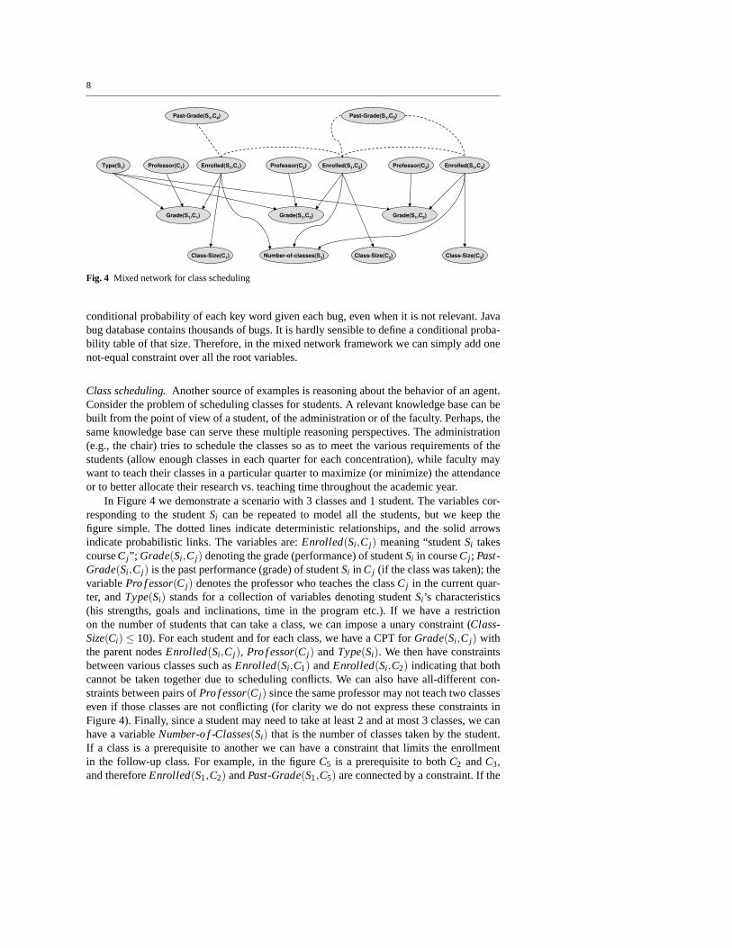
Theorem 1 (I-map) Given a mixed networkM = M(B,R) and its mixed graph GM , thenGM is a minimal I-map ofM relative to dm-separation. Namely, if< X,Z,Y >dm thenPM (X|Y,Z) = PM (X|Z) and no arc can be removed while maintaining this property.

Proof Assuming< X,Z,Y >dm we should provePM (X|Y,Z) = PM (X|Z). Namely, weshould prove thatPS(X|Y,Z,A = 1) = PS(X|Z,A = 1) , whenS= S(B,R), andA = 1 isan abbreviation to assigning all auxiliary variables inS the value 1 (Proposition 1). SinceS= S(B,R) is a regular belief network we can use the ancestral graph criterion to deter-mine d-separation. It is easy to see that the ancestral graphof the directed graph ofSgivenX ∪Y ∪ Z ∪A is identical to the corresponding ancestral mixed graph (ifwe ignore theedges going into the evidence variablesA), and thus dm-separation translates to d-separationand provides a characterization of I-mapness of mixed networks. The minimality of mixedgraphs as I-maps follows from the minimality of belief networks relative to d-separationapplied to the auxiliary network. ut

Example 3Figure 6(a) shows a regular belief network in whichX andY are d-separatedgiven the empty set. If we add a constraintRPQ betweenP andQ, we obtain the mixed net-work in Figure 6(b). According to dm-separationX is no longer independent ofY, becauseof the pathXPQY in the ancestral graph. Figure 6(c) shows the auxiliary network, with vari-ableA assigned to 1 corresponding to the constraint betweenP andQ. D-separation alsodictates a dependency betweenX andY.

We will next see the first virtue of “mixed” network when compared with the “auxiliary”network. Namely, it will allow the constraint network to be processed by any constraintpropagation algorithm to yield another, equivalent, well defined, mixed network.

Definition 9 (equivalent mixed networks)Two mixed networks defined on the same setof variablesX = {X1, ...,Xn} and the same domains,D1, ...,Dn, denoted byM1 = M(B1,R1)

and M2 = M(B2,R2), are equivalent iff they are equivalent as probability distributions,namely iffPM1 = PM2 (see Definition 3).

Proposition 2 If R1 andR2 are equivalent constraint networks (i.e., they have the same setof solutions), then for any belief networkB, M(B,R1) is equivalent toM(B,R2).

Proof The proof follows directly from Definition 3. ut

The following two propositions show that if we so desire, we can avoid redundancy orexploit redundancy by moving deterministic relations fromB to R or vice versa.

13

Proposition 3 LetB be a belief network and P(x|pax) be a deterministic CPT that can beexpressed as a constraint C(x, pax). Let B1 = B \P(x|pax). ThenM(B,φ) = M(B1,C) =M(B,C).

Proof All three mixed networksM(B,φ), M(B1,C) andM(B,C) admit the same set of tu-ples of strictly positive probability. Furthermore, the probabilities of the solution tuples aredefined by all the CPTs ofB exceptP(x|pax). Therefore, the three mixed networks areequivalent. ut

Corollary 1 Let B = 〈X,D,G,P〉 be a belief network andF a set of constraints extractedfromP. ThenM(B,φ) = M(B,F).

In conclusion, the above corollary shows one advantage of looking at mixed networksrather than at auxiliary networks. Due to the explicit representation of deterministic rela-tionships, notions such as inference and constraint propagation are naturally defined and areexploitable in mixed networks.

4 Inference and Search for Graphical Models

In this section we review the two main algorithmic approaches for graphical models: in-ference and search. Inference methods process the available information, derive and recordnew information (typically involving one less variable), and proceed in a dynamic program-ming manner until the task is solved. Search methods performreasoning by conditioning onvariable values and enumerating the entire solution space.In sections 5 and 6 we will showhow these methods apply for mixed deterministic and probabilistic networks.

4.1 Inference Methods

Most inference methods assume an ordering of the variables,that dictates the order in whichthe functions are processed. The notion ofinduced widthor treewidthis central in charac-terizing the complexity of the algorithms.

Induced graphs and induced width.An ordered graphis a pair(G,d) whereG is an undi-rected graph, andd = X1, ...,Xn is an ordering of the nodes. Thewidth of a nodein an orderedgraph is the number of the node’s neighbors that precede it inthe ordering. Thewidth of anordering d, denotedw(d), is the maximum width over all nodes. Theinduced width of anordered graph, w∗(d), is the width of the induced ordered graph obtained as follows: nodesare processed from last to first; when nodeX is processed, all its preceding neighbors areconnected. Theinduced width of a graph, w∗, is the minimal induced width over all itsorderings. Thetreewidthof a graph is the minimal induced width over all orderings.

Bucket elimination.As an example of inference methods, we will give a short review ofBucket Elimination, which is a unifying framework for variable elimination algorithms ap-plicable to probabilistic and deterministic reasoning [Bertele and Brioschi(1972), Dechterand Pearl(1987), Zhang and Poole(1994), Dechter(1996)]. The input to a bucket-eliminationalgorithm is a knowledge-base theory specified by a set of functions or relations (e.g.,clauses for propositional satisfiability, constraints, orconditional probability tables for be-lief networks). Given a variable ordering, the algorithm partitions the functions (e.g., CPTs

14

Algorithm 1 : ELIM -BEL

input : A belief networkB = {P1, ...,Pn}; an ordering of the variables,d; observationse.output : The updated beliefP(X1|e), andP(e).PartitionB into bucket1, . . ., bucketn // Initialize1for p← n down to 1 do // Backward2

Let λ1,λ2, ...,λ j be the functions inbucketpif bucketp contains evidence Xp = xp then

for i← 1 to j doAssignXp← xp in λiMove λi to the bucket of its latest variable

elseGenerateλ p = ∑Xp Π j

i=1λi

Add λ p to the bucket of its latest variable

return P(X1|e) by normalizing the product inbucket1, andP(e) as the normalizing factor.3

or constraints) into buckets, where a function is placed in the bucket of its latest argument inthe ordering. The algorithm processes each bucket, from last to first, by a variable elimina-tion procedure that computes a new function that is placed inan earlier (lower) bucket. Forbelief assessment, when the bucket does not have an observedvariable, the bucket procedurecomputes the product of all the probability tables and sums over the values of the bucket’svariable. Observed variables are independently assigned to each function and moved to thecorresponding bucket, thus avoiding the creation of new dependencies. Algorithm 1 showsElim-Bel, the bucket-elimination algorithm for belief assessment.The time and space com-plexity of such algorithms is exponential in the induced width w∗. For more information see[Dechter(1999)].

4.2 AND/OR Search Methods

As a framework for search methods, we will use the recently proposed AND/OR searchspace framework for graphical models [Dechter and Mateescu(2007)]. The usual way to dosearch (called hereOR search) is to instantiate variables in a static or dynamic order. Inthesimplest case this defines a search tree, whose nodes represent states in the space of partialassignments, and the typical depth first (DFS) algorithm searching this space would requirelinear space. If more space is available, then some of the traversed nodes can be cached,and retrieved when encountered again, and the DFS algorithmwould in this case traverse agraph rather than a tree.

The traditional OR search space however does not capture anyof the structural prop-erties of the underlying graphical model. IntroducingAND nodes into the search space cancapture the structure of the graphical model by decomposingthe problem into independentsubproblems. TheAND/OR search spaceis a well known problem solving approach de-veloped in the area of heuristic search, that exploits the problem structure to decomposethe search space. The states of an AND/OR space are of two types:ORstates which usuallyrepresent alternative ways of solving the problem (different variable values), andANDstateswhich usually represent problem decomposition into subproblems, all of which need to besolved. We will next present the AND/OR search space for a generalgraphical modelwhichin particular applies to mixed networks. The AND/OR search space is guided by a pseudotree that spans the original graphical model.

15

A

D

B C

E

f3(ABE)

f2(AB)

f4(BCD)

f1(AC)

(a) Graphical model

A

D

B

CE

(b) Pseudo tree

0

A

B

0

E C

0 1

D

0 1

D

0 1 0 1

1

E C

0 1

D

0 1

D

0 1 0 1

1

B

0

E C

0 1

D

0 1

D

0 1 0 1

1

E C

0 1

D

0 1

D

0 1 0 1

(c) Search tree

Fig. 7 AND/OR search tree

Definition 10 (pseudo tree)A pseudo treeof a graphG= (X,E) is a rooted treeT havingthe same set of nodesX, such that every edge inE is a backarc inT (i.e., it connects nodeson the same path from root).

Given a reasoning graphical modelM (e.g., belief network, constraint network, influ-ence diagram) its primal graphG and a pseudo treeT of G, the associated AND/OR tree isdefined as follows [Dechter and Mateescu(2007)].

Definition 11 (AND/OR search tree of a graphical model)Given a graphical modelM =〈X,D,F〉, its primal graphG and a pseudo treeT of G, the associated AND/OR search treehas alternating levels of OR and AND nodes. The OR nodes are labeledXi and correspondto variables. The AND nodes are labeled〈Xi ,xi〉 (or simply xi) and correspond to valueassignments. The structure of the AND/OR search tree is based onT . The root is an ORnode labeled with the root ofT . The children of an OR nodeXi are AND nodes labeledwith assignments〈Xi ,xi〉 (or xi) that are consistent with the assignments along the path fromthe root. The children of an AND node〈Xi ,xi〉 are OR nodes labeled with the children ofXi

in T . A solution subtreeof an AND/OR search graph is a subtree that: (1) contains the rootnode of the AND/OR graph; (2) if an OR node is in the subtree, then one and only one ofits children is in the subtree; (3) if an AND node is in the subtree, then all of its children arein the subtree; (4) the assignment corresponding to the solution subtree is consistent withrespect to the graphical model (i.e., it has a non-zero valuewith respect to the functions ofthe model).

Example 4Figure 7 shows an example of an AND/OR search tree. Figure 7(a) shows agraphical model defined by four functions, over binary variables, and assuming all tuples areconsistent. When some tuples are inconsistent, some of the paths in the tree do not exists.Figure 7(b) gives the pseudo tree that guides the search, from top to bottom, as indicatedby the arrows. The dotted arcs are backarcs from the primal graph. Figure 7(c) shows theAND/OR search tree, with the alternating levels of OR (circle) and AND (square) nodes,and having the structure indicated by the pseudo tree. In this case we assume that all tuplesare consistent.

The AND/OR search tree for a graphical model specializes thenotion of AND/ORsearch spaces for state-space models as defined in [Nilsson(1980)]. The AND/OR searchtree can be traversed by a depth first search algorithm, thus using linear space. It was al-ready shown [Freuder and Quinn(1985), Bodlaender and Gilbert(1991), Bayardo and Mi-ranker(1996), Darwiche(2001), Dechter and Mateescu(2004), Dechter and Mateescu(2007)]that:

16

A

D

B

CE

[ ]

[A]

[AB]

[BC]

[AB]

(a) Pseudo tree

0

A

B

0

E C

0 1

D

0 1

D

0 1 0 1

1

E C

0 1

D

0 1

D

0 1 0 1

1

B

0

E C

0 1 0 1

1

E C

0 1 0 1

(b) Context minimal graph

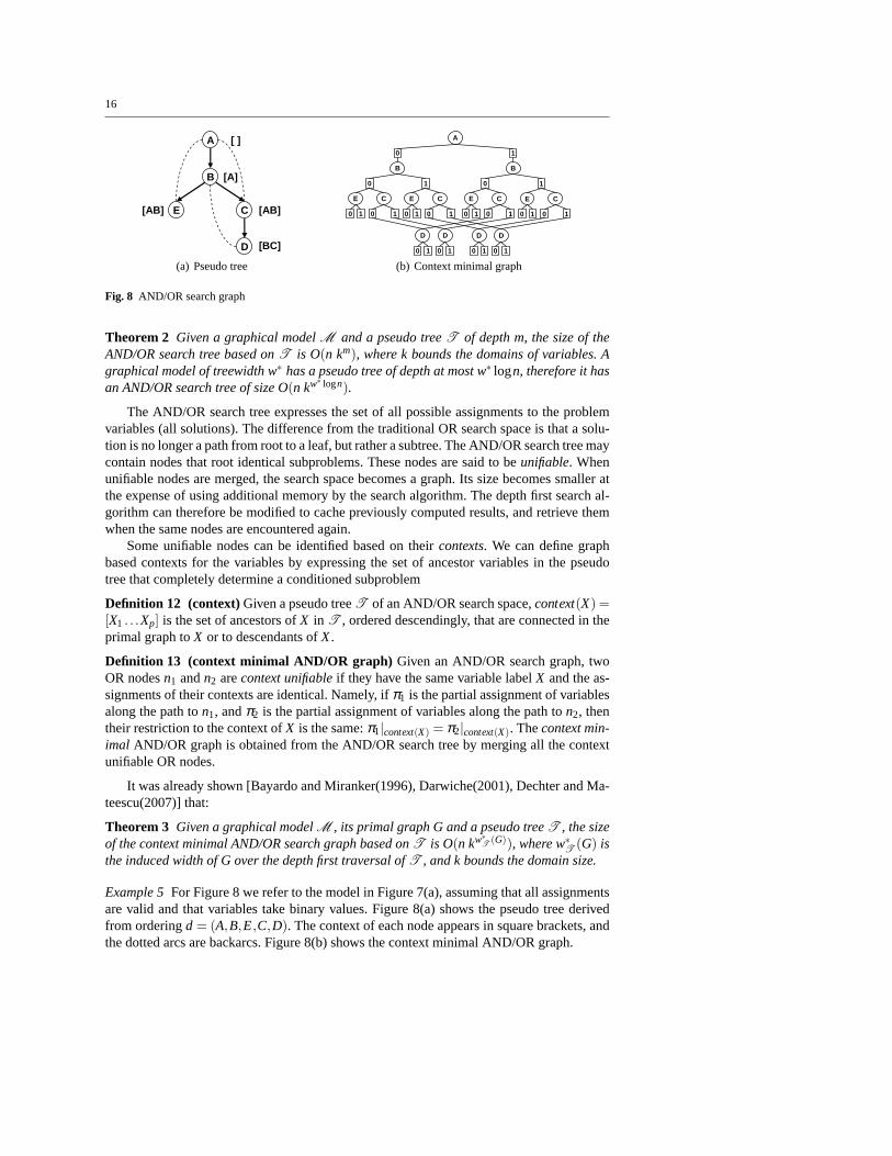
Fig. 8 AND/OR search graph

Theorem 2 Given a graphical modelM and a pseudo treeT of depth m, the size of theAND/OR search tree based onT is O(n km), where k bounds the domains of variables. Agraphical model of treewidth w∗ has a pseudo tree of depth at most w∗ logn, therefore it hasan AND/OR search tree of size O(n kw∗ logn).

The AND/OR search tree expresses the set of all possible assignments to the problemvariables (all solutions). The difference from the traditional OR search space is that a solu-tion is no longer a path from root to a leaf, but rather a subtree. The AND/OR search tree maycontain nodes that root identical subproblems. These nodesare said to beunifiable. Whenunifiable nodes are merged, the search space becomes a graph.Its size becomes smaller atthe expense of using additional memory by the search algorithm. The depth first search al-gorithm can therefore be modified to cache previously computed results, and retrieve themwhen the same nodes are encountered again.

Some unifiable nodes can be identified based on theircontexts. We can define graphbased contexts for the variables by expressing the set of ancestor variables in the pseudotree that completely determine a conditioned subproblem

Definition 12 (context)Given a pseudo treeT of an AND/OR search space,context(X) =[X1 . . .Xp] is the set of ancestors ofX in T , ordered descendingly, that are connected in theprimal graph toX or to descendants ofX.

Definition 13 (context minimal AND/OR graph) Given an AND/OR search graph, twoOR nodesn1 andn2 arecontext unifiableif they have the same variable labelX and the as-signments of their contexts are identical. Namely, ifπ1 is the partial assignment of variablesalong the path ton1, andπ2 is the partial assignment of variables along the path ton2, thentheir restriction to the context ofX is the same:π1|context(X) = π2|context(X). Thecontext min-imal AND/OR graph is obtained from the AND/OR search tree by merging all the contextunifiable OR nodes.

It was already shown [Bayardo and Miranker(1996), Darwiche(2001), Dechter and Ma-teescu(2007)] that:

Theorem 3 Given a graphical modelM , its primal graph G and a pseudo treeT , the sizeof the context minimal AND/OR search graph based onT is O(n kw∗

T(G)), where w∗

T(G) is

the induced width of G over the depth first traversal ofT , and k bounds the domain size.

Example 5For Figure 8 we refer to the model in Figure 7(a), assuming that all assignmentsare valid and that variables take binary values. Figure 8(a)shows the pseudo tree derivedfrom orderingd = (A,B,E,C,D). The context of each node appears in square brackets, andthe dotted arcs are backarcs. Figure 8(b) shows the context minimal AND/OR graph.

17

4.2.1 Weighted AND/OR graphs

In [Dechter and Mateescu(2007)] it was shown how the probability distribution of a givenbelief network can be expressed using AND/OR graphs, and howqueries of interest, suchas computing the posterior probability of a variable or the probability of the evidence, canbe computed by a depth-first search traversal. All we need is to annotate the OR-to-ANDarcs with weights derived from the relevant CPTs, such that the product of weights on thearc of any solution subtree is equal to the probability of that solution according to the beliefnetwork.

Formally, given a belief networkB = 〈X,D,G,P〉 and a pseudo treeT , the bucketof Xi relative toT , denotedBT (Xi), is the set of functions whose scopes containXi andare included inpathT (Xi), which is the set of variables from the root toXi in T . Namely,BT (Xi) = {Pj ∈P|Xi ∈ scope(Pj),scope(Pj)⊆ pathT (Xi)}. A CPT belongs to the bucket ofa variableXi iff its scope has just been fully instantiated whenXi was assigned. Combiningthe values of all functions in the bucket, for the current assignment, gives the weight of theOR-to-AND arc:

Definition 14 (OR-to-AND weights)Given an AND/OR graph of a belief networkB, theweight w(n,m)(Xi ,xi) of arc (n,m) whereXi labelsn andxi labelsm, is thecombinationofall the CPTs inBT (Xi) assigned by values along the current path to the AND nodem, πm.Formally,w(n,m)(Xi ,xi) =⊗Pj∈BT (Xi)Pj(asgn(πm)[scope(Pj)]).

Definition 15 (weight of a solution subtree)Given a weighted AND/OR graph of a beliefnetworkB, and given a solution subtreet having the OR-to-AND set of arcsarcs(t), theweight oft is defined byw(t) =⊗e∈arcs(t)w(e).

Example 6Figure 9 shows a weighted AND/OR tree for a belief network. Figure 9(a) showsthe primal graph, 9(b) is the pseudo tree, and 9(c) shows the conditional probability tables.Figure 9(d) shows the weighted AND/OR search tree. Naturally, this tree could be trans-formed into the context minimal AND/OR graph, similar to theone in Figure 8(b).

Value of a node.When solving a reasoning task, each node of the AND/OR graph can beassociated with avalue. The value could be the number of solutions restricted belowthenode, or the probability of those solutions. Whenever a subproblem is solved, the solutionvalue is recorded and pointed to by the context assignment ofthe node. Whenever the samecontext assignment is encountered again along a different path, the recorded solution valueis retrieved.

Example 7We refer again to the example in Figure 9. Considering a constraint network thatimposes thatD = 1 andE = 0 (this can also be evidence in the belief network), the traceofthe depth first search algorithm without caching (algorithmAND-OR-CPE, described laterin Section 6) is given in Figure 10. To make the computation straightforward, the consistentleaf AND nodes are given a value of 1 (shown under the square node). The final value ofeach node is shown to its left, while the OR-to-AND weights are shown close to the arcs. Thecomputation of the final value is detailed for one OR node (along the pathA = 0,B = 1,C)and one AND node (along the pathA = 1,B = 1).

In Sections 5 and 6 we will extend the inference and search algorithms to solve the CPEquery over the new framework of mixed networks.

18

A

D

B C

E

(a) Belief network

A

D

B

CE

(b) Pseudo tree

.2

.7

.5

.4

E=0

.811

.301

.510

.600

E=1BA

.1

.4

B=0

.91

.60

B=1A

.7

.2

C=0

.31

.80

C=1A

.4

.6

P(A)

1

0

A

.5

.3

.1

.2

D=0

.511

.701

.910

.800

D=1CB

P(E | A,B)P(D | B,C)

P(B | A) P(C | A)P(A)

(c) CPTs

0

A

B

0

E C

0

D

0 1

1

D

0 1

0 1

1

E C

0

D

0 1

1

D

0 1

0 1

1

B

0

E C

0

D

0 1

1

D

0 1

0 1

1

E C

0

D

0 1

1

D

0 1

0 1

.7.8 .9 .5 .7.8 .9 .5

.4 .5 .7 .2.2 .8 .2 .8 .1 .9 .1 .9

.4 .6 .1 .9

.6 .4

.6 .5 .3 .8

.2 .1 .3 .5 .2 .1 .3 .5

(d) Labeled AND/OR tree

Fig. 9 Labeled AND/OR search tree for belief networks

0

A

B

0

E C

0

D

1

1

D

1

0

1

E C

0

D

1

1

D

1

0

1

B

0

E C

0

D

1

1

D

1

0

1

E C

0

D

1

1

D

1

0

.7.8 .9 .5 .7.8 .9 .5

.4 .5 .7 .2.2 .8 .2 .8 .1 .9 .1 .9

.4 .6 .1 .9

.6 .4

.8 .9

.8 .9

.7 .5

.7 .5

.8 .9

.8 .9

.7 .5

.7 .5

.4 .5 .7 .2.88 .54 .89 .52

.352 .27 .623 .104

.3028 .1559

.3028 .1559

P(D=1,E=0) = .24408

1

1 1 1 1

1 1 1 1 1 1 1

(.2*.7) + (.8*.5)

(.2*.52)

Fig. 10 AND/OR search tree with final node values

5 Inference Algorithms for Processing Mixed Networks

We will focus on the CPE task of computingP(ϕ), whereϕ is the constraint expression orCNF formula, and show how we can answer the query using inference. A number of relatedtasks can be easily derived by changing the appropriate operator (e.g. using maximizationfor maximum probable explanation - MPE, or summation and maximization for maximuma posteriori hypothesis - MAP). The results in this section are based on the work in [Dechterand Larkin(2001)] and some of the work in [Larkin and Dechter(2003)].

5.1 Inference by Bucket Elimination

We will first derive a bucket elimination algorithm for mixednetworks when the determin-istic component is a CNF formula and latter will show how it generalizes to any constraint

19

expression. Given a mixed networkM(B,ϕ), whereϕ is a CNF formula defined on a subsetof variablesQ, theCPE task is to compute:

PB(ϕ) = ∑xQ∈models(ϕ)

P(xQ).

Using the belief network product form we get:

P(ϕ) = ∑{x|xQ∈models(ϕ)}

n

∏i=1

P(xi |xpai ).

We assume thatXn is one of the CNF variables, and we separate the summation over Xn andX \{Xn}. We denote byγn the set of all clauses that are defined onXn and byβn all the restof the clauses. The scope ofγn is denoted byQn, we defineSn = X \Qn andUn is the set ofall variables in the scopes of CPTs and clauses that are defined overXn. We get:

P(ϕ) = ∑{xn−1|xSn∈models(βn)}

∑{xn|xQn∈models(γn)}

n

∏i=1

P(xi |xpai ).

Denoting bytn the set of indices of functions in the product thatdo notmentionXn and byln = {1, . . . ,n}\ tn we get:

P(ϕ) = ∑{xn−1|xSn∈models(βn)}

∏j∈tn

Pj · ∑{xn|xQn∈models(γn)}

∏j∈ln

Pj .

Therefore:P(ϕ) = ∑

{xn−1|xSn∈models(βn)}

(∏j∈tn

Pj) ·λ Xn,

whereλ Xn is defined overUn−{Xn}, by

λ Xn = ∑{xn|xQn∈models(γn)}

∏j∈ln

Pj . (1)

The case of observed variables.WhenXn is observed, or constrained by a literal, the sum-mation operation reduces to assigning the observed value toeach of its CPTsand to eachof the relevant clauses. In this case Equation (1) becomes (assumeXn = xn andP=xn is thefunction instantiated by assigningxn to Xn):

λ xn = ∏j∈ln

Pj=xn, i f xQn ∈m(γn∧ (Xn = xn)). (2)

Otherwise,λ xn = 0. Since ¯xQn satisfiesγn ∧ (Xn = xn) only if xQn−Xn satisfiesγxn =resolve(γn,(Xn = xn)), we get:

λ xn = ∏j∈ln

Pj=xni f xQn−Xn ∈m(γxn

n ). (3)

Therefore, we can extend the case of observed variable in a natural way: CPTs are assignedthe observed value as usual while clauses are individually resolved with the unit clause(Xn = xn), and both are moved to appropriate lower buckets.

In general, when we dont have evidence in the bucket ofXn we should computeλ Xn.We need to collect all CPTs and clauses mentioningXn and then compute the functionin Equation (1). The computation of the rest of the expression proceeds withXn−1 in the

20

Algorithm 2 : ELIM -CPE

input : A belief networkB = {P1, ...,Pn}; a CNF formula onk propositionsϕ = {α1, ...αm}defined overk propositions; an ordering of the variables,d = {X1, . . . ,Xn}.

output : The beliefP(ϕ).Place buckets with unit clauses last in the ordering (to be processed first). // Initialize1PartitionB andϕ into bucket1, . . . ,bucketn, wherebucketi contains all the CPTs and clauseswhose highest variable isXi .Put each observed variable into its appropriate bucket. LetS1, ...,Sj be the scopes of the CPTs,andQ1, ...Qr be the scopes of the clauses. (We denote probabilistic functions byλs and clausesby αs).for p← n down to 1 do // Backward2

Let λ1, . . . ,λ j be the functions andα1, . . . ,αr be the clauses inbucketpProcess-bucketp(∑, (λ1, . . . ,λ j ),(α1, . . . ,αr ))

return P(ϕ) as the result of processingbucket1.3

ProcedureProcess-bucketp(⇓, (λ1, . . . ,λ j),(α1, . . . ,αr ) )

if bucketp contains evidence Xp = xp (or a unit clause)then1. AssignXp = xp to eachλi and put each resulting function in the bucket of its latestvariable2. Resolve eachαi with the unit clause, put non-tautology resolvents in the buckets of theirlatest variable andmove any bucket with unit clause to top of processing

elseGenerateλ p =⇓{xp|xUp∈models(α1,...,αr )} ∏ j

i=1 λi

Add λ p to the bucket of the latest variable inUp, whereUp =⋃ j

i=1 Si⋃r

i=1 Qi −{Xp}

same manner. This yields algorithmElim-CPE described in Algorithm 2 with ProcedureProcess-bucketp. The elimination operation is denoted by the general operator symbol⇓ that instantiates to summation for the current query.

For every ordering of the propositions, once all the CPTs andclauses are partitioned(each clause and CPT is placed in the bucket of the latest variable in their scope), the algo-rithm process the buckets from last to first. It process each bucket as eitherevidence bucket, ifwe have a unit clause (evidence), or as afunction computationbucket, otherwise. Letλ1, ...λt

be the probabilistic functions in bucketP over scopesS1, ...,St andα1, ...αr be the clausesover scopesQ1, ...,Qr . The algorithm computes a new functionλ P overUp = S∪Q−{Xp}whereS= ∪iSi , andQ = ∪ jQ j , defined by:

λ P = ∑{xp|xQ∈models(α1,...,αr )}

∏j

λ j (4)

From our derivation we can already conclude that:

Theorem 4 (correctness and completeness)Algorithm Elim-CPE is sound and completefor the CPE task.

Example 8Consider the belief network in Figure 11 and the queryϕ = (B∨C)∧ (G∨D)∧(¬D∨¬B). The initial partitioning into buckets along the orderingd = A,C,B,D,F,G, aswell as the output buckets are given in Figure 12. We compute:In bucketG: λ G( f ,d) = ∑{g|g∨d=true}P(g| f )In bucketF : λ F(b,c,d) = ∑ f P( f |b,c)λ G( f ,d)

21

A

F

B C

D

G

(a) Directed acyclic graph

A

F

B C

D

G

(b) Moral graph

Fig. 11 Belief network

Bucket G: P(G|F,D)

Bucket F: P(F|B,C)

Bucket D: P(D|A,B)

Bucket B: P(B|A)

Bucket C: P(C|A)

Bucket A: P(A)

)( CB∨ ),,( CBADλ

)( DG ∨

)( BD ¬∨¬

),( CABλ

)(ACλ

),,( DCBfλ

),( DFGλ

)(ϕP

Fig. 12 Execution of ELIM -CPE

Bucket G: P(G|F,D)

Bucket D: P(D|A,B)

Bucket B: P(B|A),P(F|B,C),

Bucket C: P(C|A)

Bucket F:

Bucket A:

)( CB∨ ),( BADλ

),( CFBλ

)(1 ABλ

G )( ¬∨ DG

D ),( ), ( DFBD Gλ¬∨¬

)(FCλ

)(2 ABλ )(ACλ Fλ

C

)(ϕP

B¬

)(FDλ

Fig. 13 Execution of ELIM -CPE (evidence¬G)

In bucketD: λ D(a,b,c) = ∑{d|¬d∨¬b=true}P(d|a,b)λ F(b,c,d)

In bucketB: λ B(a,c) = ∑{b|b∨c=true}P(b|a)λ D(a,b,c)λ F(b,c)In bucketC: λC(a) = ∑c P(c|a)λ B(a,c)In bucketA: λ A = ∑a P(a)λC(a)The result isP(ϕ) = λ A.For exampleλ G( f ,d = 0) = P(g = 1| f ), because ifd = 0 g must get the value “1”, whileλ G( f ,d = 1) = P(g = 0| f )+P(g = 1| f ).

Note that some saving due to constraints can be obtained in each function computation.Consider the bucketD that has functions over 4 variables. Brute force computation wouldrequire enumerating 16 tuples, because the algorithm has tolook at all possible assignmentsof four binary variables. However since the processing should be restricted to tuples whereb andd cannot both be true, there is a potential for restricting thecomputation to 12 tuplesonly. We will elaborate on this more later when discussing sparse function representations.

We can exploit constraints in Elim-CPE in two ways followingthe two cases for pro-cessing a bucket either as evidence-bucket, or as a function-computation bucket.

Exploiting constraints in evidence bucket.Algorithm Elim-CPE is already explicit in howit takes advantage of the constraints when processing an evidence bucket. It includes a unitresolution step whenever possible (see ProcedureProcess-bucketp) and a dynamic re-

22

ordering of the buckets that prefers processing buckets that include unit clauses. These twosteps amount to applyingunit propagationwhich is known to be a very effective constraintpropagation algorithm for processing CNF formulas. This may have a significant compu-tational impact because evidence buckets are easy to process, because unit propagation in-creases the number of buckets that will have evidence and because treating unit clauses asevidence avoids the creation new dependencies. To further illustrate the possible impact ofinferring unit clauses we look at the following example.

Example 9Let’s extend the example by adding¬G to our earlier query. This will place¬Gin the bucket ofG. When processing bucketG, unit resolution creates the unit clauseD,which is then placed in bucketD. Next, processing bucketF creates a probabilistic functionon the two variablesB andC. Processing bucketD that now contains a unit clause will assignthe valueD to the CPT in that bucket and apply unit resolution, generating the unit clause¬B that is placed in bucketB. Subsequently, in bucketB we can apply unit resolution again,generatingC placed in bucketC, and so on. In other words, aside from bucketF , we wereable to process all buckets as observed buckets, by propagating the observations. (See Figure13.) To incorporate dynamic variable ordering, after processing bucketG, we move bucketD to the top of the processing list (since it has a unit clause).Then, following its processing,we process bucketB and then bucketC, thenF , and finallyA.

Exploiting constraints in function computation. Sometimes there is substantial determin-ism present in a network that cannot yield a significant amount of unit clauses or shrinkthe domains of variables. For example, consider the case when the network is completelyconnected with equality constraints. Any domain value for any single variable is feasible,but there are still onlyk solutions, wherek is the domain size. We can still exploit suchconstraints in the function-computation. To facilitate this we may need to consider differentdata structures, other than tables, to represent the CPT functions.

In [Larkin and Dechter(2003)] we focused on this aspect of exploiting constraints. Wepresented the bucket-elimination algorithm calledElim-Sparsefor the CPE query, that usesa sparse representation of the CPT functions as a relation. Specifically, instead of recordinga table as large as the product of the domain sizes of all the variables, a function is main-tained as a relation of non-zero probability tuples. In the above example, with the equalityconstraints, defining the function as a table would require atable of sizekn wheren is thenumber of variables in the scope of the function, but onlynk (k tuples of sizen each) asa relation. Efficient operations to work with these functions are also available. These aremainly based on the Hash-Join procedure which is well-knownin database theory [Korthand Silberschatz(1991)] as described in [Larkin and Dechter(2003)].

In Elim-Sparse, the constraints are absorbed into the (relation-based) CPTs (e.g., in ageneralized arc-consistency manner) and then relational operators can be applied. Alter-natively, one can also devise efficient function-computation procedures using constraint-based search schemes. We will assume the sparse function representation explicitly in theconstraint-based CPE algorithmElim-ConsPE(i)described in section 5.2.2.

5.2 Extensions of Elim-CPE

Unit propagation and any higher level of constraint processing can also be applied a priorion the CNF formula before we apply Elim-CPE. This can yield stronger CNF expressionsin each bucket with more unit clauses. This can also improve the function computation innon-evidence buckets. Elim-CPE(i) is discussed next.

23

5.2.1 Elim-CPE(i)

One form of constraint propagation is bounded resolution [Rish and Dechter(2000)]. It ap-plies pair-wise resolution to any two clauses in the CNF theory iff the resolvent size does notexceed a bounding parameter,i. Bounded-resolution algorithms can be applied until quies-cence or in a directional manner, calledBDR(i). After partitioning the clauses into orderedbuckets, each one is processed by resolution relative to thebucket’s variable, with boundi.

This suggests extending Elim-CPE into a parameterized family of algorithms Elim-CPE(i) that incorporatesBDR(i). All we need is to include ProcedureBDR(i) describedbelow in the “else” branch of the ProcedureProcess-bucketp.

ProcedureBDR(i)

if the bucket does not have an observed variablethenfor each pair{(α ∨Q j ),(β ∨¬Q j )} ⊆ bucketp do

if the resolventγ = α ∪β contains no more than i propositionsthenplace the resolvent in the bucket of its latest variable

5.2.2 Probability of Relational Constraints

When the variables in the belief network are multi-valued, the deterministic query can beexpressed using a constraint expression with relational operators. The set of solutions of aconstraint network can be expressed using the join operator. The join of two relationsRAB

andRBC denotedRAB 1 RBC is the largest set of solutions overA,B,C satisfying the twoconstraintsRAB andRBC. The set of solutions of the constraint expressionR = {R1, ...Rt} issol(R) =1

ti=1 Ri .

Given a belief network and a constraint expressionR we may be interested in computingP(x∈ sol(R)). A bucket-elimination algorithm for computing this task isa simple general-ization of Elim-CPE, except that it uses the relational operators as expressed in Algorithm 4.Algorithm Elim-ConsPE uses the notion of arc-consistency which generalizes unit propaga-tion and it is also parameterized to allow higher levels of directionali-consistency (DIC(i))[Dechter(2003)], generalizingBDR(i) (see step 1 of the ”else” part of theprocess-bucket-relprocedure). The algorithm assumes sparse function representation and constraint-exploitingcomputation for the bucket-functions.

Clearly, in both Elim-CPE(i) and its generalized constraint-based version Elim-ConsPE(i), higher levels of constraint propagation may desirably infer more unit and non-unit clauses. They may also require more computation however and it is hard to assess inadvance what level ofi will be cost-effective. It is known that the complexity ofBDR(i)andDIC(i) areO(exp(i)) and therefore, for small levels ofi the computation is likely to bedominated by generating the probabilistic function ratherthan byBDR(i).

Moreover, whether or not we use high level of directional consistency to yield moreevidence, a full level of directional consistency is achieved anyway by the function compu-tation. In other words, the set of positive tuples generatedin each bucket’s function compu-tation is identical to the set of consistent tuples that would have been generated by full di-rectional consistency (also known asadaptive-consistencyor directional-consistency) withthe same set of constraints. Thus, full directionali-consistency is not necessary for the sakeof function computation. It can still help inferring significantly more unit clauses (evidence)over the constraints, requiring a factor of 2 at the most for the processing of each bucket.

24

Algorithm 4 : ELIM -CONSPE

input : A belief networkB = {P1, ...,Pn} wherePi ’s are assume to have a sparserepresentation; A constraint expression overk variables,R = {RQ1 , ...,RQt } anorderingd = {X1, . . . ,Xn}

output : The beliefP(R).Place buckets with observed variables last ind (to be processed first) // Initialize1PartitionB andR into bucket1, . . . ,bucketn, wherebucketi contains all CPTs and constraintswhose highest variable isXiLet S1, ...,Sj be the scopes of the CPTs, andQ1, ...Qt be the scopes of the constraints.We denote probabilistic functions asλs and constraints byRsfor p← n down to 1 do // Backward2

Let λ1, . . . ,λ j be the functions andR1, . . . ,Rr be the constraints inbucketpProcess-bucket-RELp(∑, (λ1, . . . ,λ j ),(R1, . . . ,Rr ))

return P(R) as the result of processingbucket1.3

ProcedureProcess-bucket-RELp(⇓, (λ1, . . . ,λ j),(R1, . . . ,Rr ) )

if bucketp contains evidence Xp = xp then1. AssignXp = xp to eachλi and put each resulting function in the bucket of its latestvariable2. Apply arc-consistency (or any constraint propagation) over the constraints in the bucket.Put the resulting constraints in the buckets of their latestvariable andmove any bucketwith single domain to top of processing

else1. Apply directionali-consistency (DIC(i))2. Generateλ p = ∑{xp|xUp∈./ j Rj }∏ j

i=1 λi with specialized sparse operations or search-basedmethods.Add λ p to the bucket of the latest variable inUp, whereUp =

⋃ ji=1 Si

⋃ri=1 Qi −{Xp}

5.3 Complexity

As usual, the worst-case complexity of bucket elimination algorithms is related to the num-ber of variables appearing in each bucket, both in the scopesof probability functions aswell as in the scopes of constraints [Dechter(1999)]. The worst-case complexity is timeand space exponential in the maximal number of variables in abucket, which is capturedby the induced-width of the relevant graph. Therefore, the complexity of Elim-CPE andElim-ConsPE isO(r ·exp(w∗)), wherew∗ is the induced width of the moral mixed orderedgraph andr is the total number of functions [Kask et al(2005)Kask, Dechter, Larrosa, andDechter]. In Figure 14 we see that while the induced width of the moral graph of the beliefnetwork is just 2 (Figure 14(a)), the induced width of the mixed graph of our example is 3(Figure 14(b)).

We can refine the above analysis to capture the role of constraints in generating unitclauses by constraint propagation. We can also try to capture the power of constraint-basedpruning obtained in function computation. To capture the simplification associated with ob-served variables, we will use the notion of anadjusted induced graph. The adjusted inducedgraph is created by processing the variables from last to first in the given ordering and con-necting the parents of each non-observed variables, only. The adjusted induced width is thewidth of the adjusted induced-graph. Figure 14(c) shows theadjusted induced-graph relativeto the evidence¬G. We see that the induced width, adjusted for this observation, is just 2

25

G

F

D

B

C

A

G

F

D

B

C

A

G

F

D

B

C

A

(a) (b) (c)

Fig. 14 Induced graphs: (a) moral graph; (b) mixed graph; (c) adjusted(for ¬G) graph

(Figure 14(c)). Notice that adjusted induced-width can be computed once we observe theevidence set obtained as a result of our propagation algorithm. In summary:

Theorem 5 ([Dechter and Larkin(2001)])Given a mixed network,M , of a belief networkover n variables, a constraint expression and an ordering o,algorithm Elim-CPE is time andspace O(n ·exp(w∗

M(o))), where w∗

M(o) is the width along o of the adjusted moral mixed

induced graph.

Capturing in our analysis the efficiency obtained when exploiting constraints infunction-computation is harder. The overall complexity depends on the amount of deter-minism in the problem. If enough is present to yield small relational CPTs, it can be fairlyefficient, but if not, the overhead of manipulating nearly full tuple lists can be larger thanwhen dealing with a table. Other structured function representations, such as decision trees[Boutilier et al(1996)Boutilier, Friedman, Goldszmidt, and Koller] or rule-based systems[Poole(1997)] might also be appropriate for sparse representation of the CPTs.

6 AND/OR Search Algorithms For Mixed Networks

Proposition 2 ensures the equivalence of mixed networks defined by one belief network andby different constraint networks that are equivalent (i.e., that have the same set of solutions).In particular, this implies that we can process the deterministic information separately (e.g.,by enforcing some consistency level, which results in a tighter representation), without los-ing any solution. Conditioning algorithms (search) offer anatural approach for exploitingconstraints. The intuitive idea is to search in the space of partial variable assignments, anduse the wide range of readily available constraint processing techniques to limit the actualtraversed space. We will describe the basic principles in the context of AND/OR searchspaces [Dechter and Mateescu(2007)]. We will first describethe AND-OR-CPEAlgorithm.Then, we will discuss how to incorporate in AND-OR-CPE techniques exploiting deter-minism, such as: (1) constraint propagation (look-ahead),(2) backjumping and (3) good andnogood learning.

26

Algorithm 5 : AND-OR-CPE

input : A mixed networkM = 〈X,D,G,P,C〉; a pseudo treeT of the moral mixed graph,rooted atX1; parentspai (OR-context) for every variableXi ; caching set totrue orf alse.

output : The probabilityP(x∈ ρ(R)) that a tuple satisfies the constraint query.if caching == true then // Initialize cache tables1

Initialize cache tables with entries of “−1”2

v(X1)← 0; OPEN←{X1} // Initialize the stack OPEN3while OPEN 6= φ do4

n← top(OPEN); removen from OPEN5if caching == trueand n is OR, labeled Xi andCache(asgn(πn)[pai ]) 6=−1 then // If6in cache

v(n)←Cache(asgn(πn)[pai ]) // Retrieve value7successors(n)← φ // No need to expand below8

else // Expand search (forward)9if n is an OR node labeled Xi then // OR-expand10

successors(n)← ConstraintPropagation(〈X,D,C〉,asgn(πn))11

// CONSTRAINT PROPAGATIONv(〈Xi ,xi〉)← ∏

f∈BT (Xi )f (asgn(πn)[pai ]), for all 〈Xi ,xi〉 ∈ successors(n)

12

if n is an AND node labeled〈Xi ,xi〉 then // AND-expand13successors(n)← childrenT (Xi)14v(Xi)← 0 for all Xi ∈ successors(n)15

Add successors(n) to top ofOPEN16

while successors(n) == φ do // Update values (backtrack)17if n is an OR node labeled Xi then18

if Xi == X1 then // Search is complete19return v(n)20

if caching == true then21Cache(asgn(πn)[pai ])← v(n) // Save in cache22

let p be the parent ofn23v(p)← v(p)∗v(n)24if v(p) == 0 then // Check if p is dead-end25

removesuccessors(p) from OPEN26successors(p)← φ27

if n is an AND node labeled〈Xi ,xi〉 then28let p be the parent ofn29v(p)← v(p)+v(n);30

removen from successors(p)31n← p32

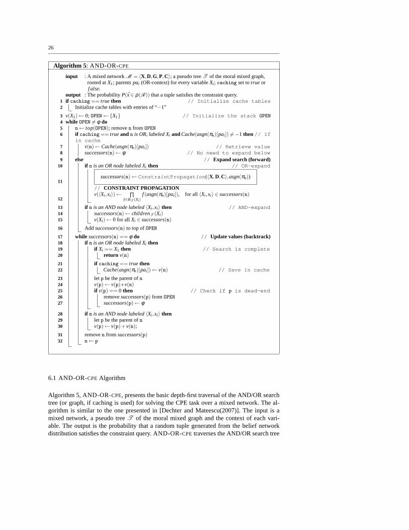
6.1 AND-OR-CPEAlgorithm

Algorithm 5, AND-OR-CPE, presents the basic depth-first traversal of the AND/OR searchtree (or graph, if caching is used) for solving the CPE task over a mixed network. The al-gorithm is similar to the one presented in [Dechter and Mateescu(2007)]. The input is amixed network, a pseudo treeT of the moral mixed graph and the context of each vari-able. The output is the probability that a random tuple generated from the belief networkdistribution satisfies the constraint query. AND-OR-CPE traverses the AND/OR search tree

27

ProcedureConstraintPropagation(R, xi)

input : A constraint networkR = 〈X,D,C〉; a partial assignment path ¯xi to variableXi .output : reduced domainDi of Xi ; reduced domains of future variables; newly inferred

constraints.This is a generic procedure that performs the desired level ofconstraint propagation, forexample forward checking, unit propagation, arc consistency over the constraint networkR andconditioned on ¯xi .return reduced domain of Xi

0

A

B

0

E C

1

D

1

0

1

E C

1

D

0 1

0 1

1

B

0

E C

0

D

1

1

D

1

0

1

E C

0

D

0 1

1

D

0 1

0 1

.9 .5 .7.8 .9 .5

.4 .5 .7 .2.8 .8 .1 .9 .1 .9

.4 .6 .1 .9

.6 .4

.5 .8

.5 .3 .5

.9

.9

1

1

.8 .9

.8 .9

1 1

1 1

.4 1 .7 1.72 .8 .89 1

.288 .8 .623 1

.5952 .9623

P( (A ∨∨∨∨ C) ∧∧∧∧ (B ∨∨∨∨ ⌉⌉⌉⌉ E) ∧∧∧∧ (B ∨∨∨∨ D) ) = .74204

.5952 .9623

Fig. 15 Mixed network defined by the queryϕ = (A∨C)∧ (B∨¬E)∧ (B∨D)

or graph corresponding toT in a DFS manner. Each node maintains a valuev which ac-cumulates the computation resulted from its subtree. OR nodes accumulate the summationof the product between each child’s value and its OR-to-AND weight, while AND nodesaccumulate the product of their children’s values. For moreinformation see [Dechter andMateescu(2007)].

Example 10We refer back to the example in Figure 9. Consider a constraint network thatis defined by the CNF formulaϕ = (A∨C)∧ (B∨¬E)∧ (B∨D). The trace of algorithmAND-OR-CPE without caching is given in Figure 15. Notice that the clause(A∨C) is notsatisfied ifA = 0 andC = 0, therefore the paths that contain this assignment cannot be partof a solution of the mixed network. The value of each node is shown to its left (the leafnodes assume a dummy value of 1, not shown in the figure). The value of the root node isthe probability ofϕ. Figure 15 is similar to Figure 10. In Figure 10 the evidence can bemodeled as the CNF formula with unit clausesD∧¬E.

The following theorems are implied immediately from the general properties ofAND/OR search algorithms [Dechter and Mateescu(2007)].

Theorem 6 AlgorithmAND-OR-CPE is sound and exact for the CPE task.

Theorem 7 Given a mixed networkM with n variables having domain sizes bounded byk and a pseudo treeT of depth m of its moral mixed graph, the time complexity ofAND-OR-CPEwith no caching is O(n·km), while the space required is linear. A mixed network oftreewidth w∗ has an AND/OR search tree whose size is O(exp(w∗ · logn)).

6.2 Constraint Propagation in AND-OR-CPE

As we already observed, Proposition 2 provides an importantjustification for using mixednetworks as opposed to auxiliary networks. The constraint portion can be processed by a

28

wide range of constraint processing techniques, both statically before search or dynamicallyduring search [Dechter(2003)].

We discuss here the use of constraint propagation during search, also known as look-ahead. This is a well known idea used in any constraint or SAT solver. In general, constraintpropagation helps to discover (using limited computation)what variable and what value toinstantiate next. The incorporation of these methods on topof AND/OR search is straight-forward. For illustration, we will only consider a static variable ordering, based on a pseudotree.

In Algorithm AND-OR-CPE, line 11 contains a call to the genericConstraintPropagation procedure consulting only the constraint subnetworkR, conditioned on the current partial assignment. The constraint propagation is relativeto the current set of constraints, the given path that definesthe current partial assignment,and the newly inferred constraints, if any, that were learned during the search. Using apolynomial time algorithm,ConstraintPropagation may discover some variablevalues that cannot be extended to a full solution. These values in the domain of a variablesare marked as inconsistent and can be removed from the current domain of the variable.All the remaining values are returned by the procedure as good candidates to extend thesearch frontier. Of course, not all the values returned byConstraintPropagation areguaranteed to lead to a solution.

We therefore have the freedom to employ any procedure for checking the consistency ofthe constraints of the mixed network. The simplest case is when no constraint propagationis used, and only the initial constraints ofR are checked for consistency, and we denote thisalgorithm by AO-C.

In the empirical evaluation, we used two forms of constraintpropagation on top of AO-C. The first, yielding algorithm AO-FC, is based onforward checking, which is one ofthe weakest forms of propagation. It propagates the effect of a value selection to each fu-ture uninstantiated variable separately, and checks consistency against the constraints whosescope would become fully instantiated by just one such future variable.

The second algorithm we used is called AO-RFC, and performs avariant ofrelationalforward checking. Rather than checking only constraints whose scope becomesfully as-signed, AO-RFC checks all the existing constraints by looking at their projection on thecurrent path. If the projection is empty an inconsistency isdetected. AO-RFC is computa-tionally more expensive than AO-FC, but its search space is smaller.

SAT solvers.One possibility that was explored with success (e.g., [Allen and Dar-wiche(2003)]) is to delegate the constraint processing to aseparate off-the-shelf SAT solver.In this case, for each new variable assignment the constraint portion is packed and fed intothe SAT solver. If no solution is reported, then that value isa dead-end. If a solution is foundby the SAT solver, then the AND/OR search continues (remember that for some tasks wemay have to traverse all the solutions of the graphical model, so the one solution found bythe SAT solver does not finish the task). The worst-case complexity of this level of constraintprocessing, at each node, is exponential.

The popular variant ofunit propagationthat was exploited in Elim-CPE can be effectivehere too. This can also be implemented by the unit resolutionengine of an available SATsolver. Such hybrid use of search and a specialized efficientSAT (or constraint) solver canbe very useful, and it underlines further the power that the mixed network representation hasin delimiting the constraint portion from the belief network.

29

A

D

B C

E F

G H I K

(a) Belief network

A

D

B C

E F

G H I K

>

>

>

>>

>> >

>

(b) Constraint network

1 2

A

C

3 4

B B

2 3 4

ED

3 4 3 4

HG

4 4

G I

4

I

D

4

G

D

2 3 4

FF

4

K

F

4

K

3

K

4

3 4

4

G

D D

B

4

D

B

OR

AND

OR

AND

OR

AND

AND

OR

(c) Constraint checking

1 2

A

C

3

B B

2 3

ED

3 3

HG

4 4

I

4

D

2 3

FF

3

K

4

3

D

B

OR

AND

OR

AND

OR

AND

AND

OR

(d) Forward checking

1

A

CB

2

ED

3 3

HG

4 4

I

4

2

F

3

K

4

OR

AND

OR

AND

OR

AND

AND

OR

(e) Maintaining arc consistency

Fig. 16 Traces of AND-OR-CPEwith various levels of constraint propagation

Example 11Figure 16(a) shows the belief part of a mixed network, and Figure 16(b) theconstraint part. All variables have the same domain,{1,2,3,4}, and the constraints express“less than” relations. Figure 16(c) shows the search space of AO-C. Figure 16(d) shows thespace traversed by AO-FC. Figure 16(e) shows the space when consistency is enforced withMaintaining Arc Consistency (which enforces full arc-consistency after each new instantia-tion of a variable).

6.3 Backjumping

Backjumping algorithms [Gaschnig(1979), Prosser(1993),Bayardo and Miranker(1996),Dechter(2003)] are backtracking search algorithms applied to the OR space, which usesthe problem structure to jump back from a dead-end as far backas possible. They have beenknown for a long time in the constraint processing community. For probabilistic models,backjumping is very useful in the context of determinism.

In graph-based backjumping(GBJ) each variable maintains a graph-based induced an-cestor set which ensures that no solutions are missed by jumping back to its deepest vari-able. If the ordering of the OR space is a DFS ordering of the primal graph, it is known[Dechter(2003)] that all the backjumps are from a variable to its DFS parent. In [Mateescu

30

4 61

3 2 7 5

8

2 7

1

4

3 5

6

8

(a)

(b) (c)

2

6

1

4

3

5

7

8

(d)

2

6

1

4

3

5

7

8

Fig. 17 Graph-based backjumping and AND/OR search

and Dechter(2005)] it was shown that this means that a simpleAND/OR search automat-ically incorporates graph-based backjumping, when the pseudo tree is a DFS tree of theprimal graph.

When the pseudo tree is not a DFS tree of the primal graph, it may happen that the parentof a node in the pseudo tree is not the node where graph-based backjumping would retreat inthe case of OR search. An example is provided in Figure 17. Figure 17a shows a graphicalmodel, 17b a pseudo tree and 17c a chain driving the OR search (top down). If a dead-endis encountered at variable 3, graph-based backjumping retreats to 8 (see 17c), while simpleAND/OR would retreat to 1, the pseudo tree parent. When the dead-end is encountered at 2,both algorithms backtrack to 3 and then to 1. Therefore, in such cases, augmenting AND/ORwith a graph-based backjumping mechanism can provide some improvement.

We want to emphasize that the graph-based backjumping behavior is in most cases in-trinsic to AND/OR search. The more advanced and computationally intensive forms of con-flict directed backjumping [Prosser(1993), Dechter(2003)] are not captured by the AND/ORgraph, and can be implemented on top of it by analyzing the constraint portion only.

6.4 Good and Nogood Learning

When a search algorithm encounters a dead-end, it can use different techniques to identifythe ancestor variable assignments that caused the dead-end, called a conflict-set. It is con-ceivable that the same assignment of that set of ancestor variables may be encountered inthe future, and they would lead to the same dead-end. Rather than rediscovering it again, ifmemory allows, it is useful to record the dead-end conflict-set as a new constraint (or clause)over the ancestor set that is responsible for it. Recording dead-end conflict-sets is sometimescalled nogood learning.

One form of nogood learning is graph-based, and it uses the same technique as graph-based backjumping to identify the ancestor variables that generate the nogood. The informa-tion on conflicts is generated from the primal graph information alone. Similar to the caseof backjumping, it is easy to see that AND/OR search already provides this information inthe context of the nodes. Therefore saving the information about the nogoods encounteredamounts to graph-based nogood learning in the case of OR search.

If deeper types of nogood learning are desirable, they need to be implemented on topof the AND/OR search. In such a case, a smaller set than the context of a node may beidentified as a culprit assignment, and may help discover future dead-ends much earlier than

31

when context-based caching alone is used. Needless to say, deep learning is computationallymore expensive and it can be facilitated via a focus on the constraint portion of the mixednetwork.

Traversing the context-based AND/OR graph can be understood as learning (and sav-ing) not only the nogoods but also their logical counterparts, thegoods(namely the consis-tent assignments). This is a feature that was proposed in recent years by several schemes[Darwiche(2001), Sang et al(2004)Sang, Bacchus, Beam, Kautz, and Pitassi, Dechter andMateescu(2007)]. This is in fact the well known technique ofcaching that became appeal-ing recently due to the availability of computer memory, when the task to be solved requiresthe enumeration of many solutions. The idea is to store the value of a solved conditionedsubproblem, associating it with a minimal set of ancestor assignments that are guaranteedto root the same conditioned subproblem, and retrieve that value whenever the same set ofancestor assignments is encountered again during search.

7 Empirical Evaluation

In this section we present an empirical evaluation of the inference and AND/OR searchmethods discussed in the previous sections.Exploiting determinism in BE vs. search.We do not advocate here that one type of al-gorithms is better than the other. In fact, as an extension ofthe results in [Mateescu andDechter(2005)], it can be shown that search and inference are in general incomparable,when both are equipped with determinism exploiting tools. Like AND/OR search, bucket-elimination that uses sparse function representation can be shown to also traverse the contextminimal AND/OR graph, but in a different direction and assuming a different control strat-egy. Inference is bottom up and breadth first, while AND/OR search is top down and depthfirst. As a result, we can imagine mixed networks where the determinism reveals itself closeto the root of the pseudo tree, making the job of AND/OR searcheasier, while Bucket Elim-ination has to traverse all the layers bottom up, only to discover that most of the messages ithas processed contain invalid tuples. Another example could show the opposite: if the deter-minism is closer to the leaves of the pseudo tree, then the performance of the two methodsis reversed.

We should emphasize again that in making this claim about inference we assume that theCPTs use a sparse representation. In practice the impact of determinism would be manifestedin generating tight functions that are sent from one bucket to another. If we consider the casediscussed after Example 8, a full table representation for four binary variables would contain16 tuples, but a restriction to only the valid tuples might bea relational representation foronly 12 of them.

Because, as explained, inference and search are in general incomparable, we will offeran experimental evaluation of each type separately, evaluating the advantages of expressingand exploiting the constraint portion separately as part ofthe mixed network framework.

7.1 Inference Algorithms

We compared empirically five algorithms: (1) Elim-CPE (which is the same as Elim-CPE(0),which does no constraint propagation except for unit propagation); (2) Elim-CPE(i); (3)Elim-CPE-D (which derives CNF clauses from mixed CPTs and then applies Elim-CPE);

32

Fig. 18 Random networks; 48 instances; network parameters< 80,4,0.75> and query parameters< 0,10>

Table 1 Insurance network (27 variables); 50 test instances; queryparameters< 20,5 >

Algorithm Time mf C. U. F.

Elim-CPE-D: 48 8 210 1 302Elim-CPE(15): 64 9 12 1 0Elim-CPE(0): 61 9 6 0 0Elim-Hidden: 104 10 0 0 0

(4) Elim-Hidden (this algorithm expresses each clause as a CPT with a new hidden vari-able, adds evidence to the hidden nodes and performs the variable elimination algorithm).All these algorithms assume that the CPTs are implemented astables, with no sparse rep-resentation. The fifth algorithm we tested is Elim-Sparse that uses a sparse relational rep-resentation of the CPTs. We tested the algorithms on some random networks, as well asrealistic networks: Insurance, Water, Mildew, Hailfinder,Munin1 and Diabetes. All algo-rithms use min-degree order, computed by repeatedly removing the node with the lowestdegree from the graph and connecting all its neighbors. For more information see [Dechterand Larkin(2001)].

The generator of random networks that we used is divided in two parts. The first createsa random belief network using a tuple< n, f ,d > as a parameter, wheren is the numberof variables,f is the maximum family size, andd is the fraction of deterministic entries inCPTs. Parents are chosen at random from the preceding variables in a fixed ordering. Theentries of the CPTs are filled in randomly. The second part generates a 3-CNF query using apair of parameters< c,e> wherec is the number of 3-CNF clauses (clauses are randomlychosen and each is given a random truth value) ande is the number of observations.

We first show a comparison of Elim-CPE-D and Elim-CPE on some random networks,in Figure 18. As mentioned before, the difference between the two algorithms is that Elim-CPE-D extracts deterministic information from CPTs. The figure shows a scatter plot ofrunning times measured in seconds. The results show that extracting deterministic informa-tion is beneficial on these instances.

We tested the algorithms on the Insurance network, which is arealistic network forevaluating car insurance risks that contains deterministic information. It has 27 variables.In the experiments reported in Table 1, Elim-CPE-D outperformed Elim-CPE substantially.Figure 19 contrasts Elim-CPE with Elim-Hidden on the Insurance network.

We also tried the Hailfinder network, another benchmark thathas 56 variables and in-cludes deterministic information. It is a normative systemthat forecasts severe summer hail

33

Table 2 Hailfinder network (56 variables); 50 test instances; queryparameters< 15,15>

Algorithm Time mf C. U. F.

Elim-CPE-D: 4 4 269 1 501Elim-CPE(15): 16 6 7 1 0Elim-CPE(0): 16 6 7 1 0Elim-Hidden: 33 7 0 0 0

Fig. 19 Insurance network; 50 test instances; query parameters< 15,5 >

Table 3 Average Times

Network EB EC ES B/S C/S

Insurance 3.56 1.05 0.24 14.83 4.38Water 4.65 3.22 0.29 16.03 11.10Mildew 7.64 4.51 0.94 8.15 4.81Hailfinder 1.99 1.14 0.99 2.01 1.15Munin1 15.92 3.58 0.84 18.95 4.26Diabetes 18.77 12.20 9.67 1.94 1.26

in northeast Colorado. The results are reported in Table 2. Here again the results are con-sistent with earlier observations that Elim-CPE-D was the most efficient. In both of thesenetworks we have determinism created by the network and the query.

We also present here some results that include the algorithmElim-Sparse [Larkin andDechter(2003)], where the CPTs are represented in relational form, by storing only the validtuples. Table 3 shows a comparison of Elim-Bel (EB), Elim-CPE (EC) and Elim-Sparse(ES). We generated 50 random queries for each network, testing the three algorithms oneach. The last two columns show the ratio of times of Elim-Belto Elim-Sparse (B/S), andof Elim-CPE to Elim-Sparse (C/S). Elim-Sparse was considerably faster than Elim-CPEon Insurance, Water, Mildew, and Munin1 (by a factor of 4 or more), but less so on Hail-finder and Diabetes (less than twice as fast). In general Elim-Sparse is more efficient thanElim-CPE especially with increasing determinism. However, the high constant factor due tomanipulation of tuple lists may prove to be too big an overhead for low determinism.

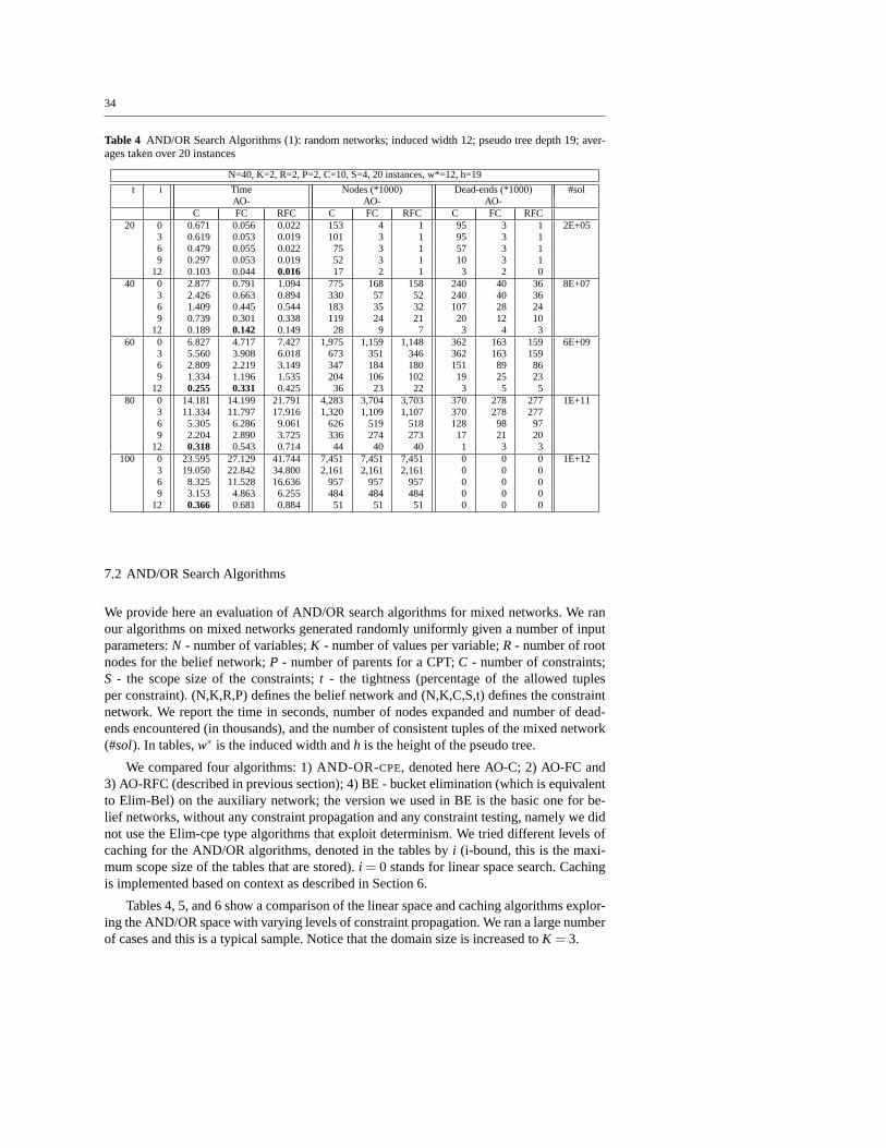
34

Table 4 AND/OR Search Algorithms (1): random networks; induced width 12; pseudo tree depth 19; aver-ages taken over 20 instances

N=40, K=2, R=2, P=2, C=10, S=4, 20 instances, w*=12, h=19

t i Time Nodes (*1000) Dead-ends (*1000) #solAO- AO- AO-

C FC RFC C FC RFC C FC RFC20 0 0.671 0.056 0.022 153 4 1 95 3 1 2E+05

3 0.619 0.053 0.019 101 3 1 95 3 16 0.479 0.055 0.022 75 3 1 57 3 19 0.297 0.053 0.019 52 3 1 10 3 1

12 0.103 0.044 0.016 17 2 1 3 2 040 0 2.877 0.791 1.094 775 168 158 240 40 36 8E+07

3 2.426 0.663 0.894 330 57 52 240 40 366 1.409 0.445 0.544 183 35 32 107 28 249 0.739 0.301 0.338 119 24 21 20 12 10

12 0.189 0.142 0.149 28 9 7 3 4 360 0 6.827 4.717 7.427 1,975 1,159 1,148 362 163 159 6E+09

3 5.560 3.908 6.018 673 351 346 362 163 1596 2.809 2.219 3.149 347 184 180 151 89 869 1.334 1.196 1.535 204 106 102 19 25 23

12 0.255 0.331 0.425 36 23 22 3 5 580 0 14.181 14.199 21.791 4,283 3,704 3,703 370 278 277 1E+11

3 11.334 11.797 17.916 1,320 1,109 1,107 370 278 2776 5.305 6.286 9.061 626 519 518 128 98 979 2.204 2.890 3.725 336 274 273 17 21 20

12 0.318 0.543 0.714 44 40 40 1 3 3100 0 23.595 27.129 41.744 7,451 7,451 7,451 0 0 0 1E+12

3 19.050 22.842 34.800 2,161 2,161 2,161 0 0 06 8.325 11.528 16.636 957 957 957 0 0 09 3.153 4.863 6.255 484 484 484 0 0 0

12 0.366 0.681 0.884 51 51 51 0 0 0

7.2 AND/OR Search Algorithms

We provide here an evaluation of AND/OR search algorithms for mixed networks. We ranour algorithms on mixed networks generated randomly uniformly given a number of inputparameters:N - number of variables;K - number of values per variable;R - number of rootnodes for the belief network;P - number of parents for a CPT;C - number of constraints;S - the scope size of the constraints;t - the tightness (percentage of the allowed tuplesper constraint). (N,K,R,P) defines the belief network and (N,K,C,S,t) defines the constraintnetwork. We report the time in seconds, number of nodes expanded and number of dead-ends encountered (in thousands), and the number of consistent tuples of the mixed network(#sol). In tables,w∗ is the induced width andh is the height of the pseudo tree.

We compared four algorithms: 1) AND-OR-CPE, denoted here AO-C; 2) AO-FC and3) AO-RFC (described in previous section); 4) BE - bucket elimination (which is equivalentto Elim-Bel) on the auxiliary network; the version we used inBE is the basic one for be-lief networks, without any constraint propagation and any constraint testing, namely we didnot use the Elim-cpe type algorithms that exploit determinism. We tried different levels ofcaching for the AND/OR algorithms, denoted in the tables byi (i-bound, this is the maxi-mum scope size of the tables that are stored).i = 0 stands for linear space search. Cachingis implemented based on context as described in Section 6.

Tables 4, 5, and 6 show a comparison of the linear space and caching algorithms explor-ing the AND/OR space with varying levels of constraint propagation. We ran a large numberof cases and this is a typical sample. Notice that the domain size is increased toK = 3.

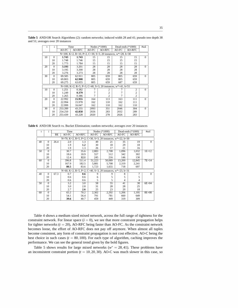
35

Table 5 AND/OR Search Algorithms (2): random networks; induced width 28 and 41; pseudo tree depth 38and 51; averages over 20 instances

t i Time Nodes (*1000) Dead-ends (*1000) #solAO-FC AO-RFC AO-FC AO-RFC AO-FC AO-RFC

N=100, K=2, R=10, P=2, C=30, S=3, 20 instances, w*=28, h=3810 0 1.743 1.743 15 15 15 15 0

10 1.748 1.746 15 15 15 1520 1.773 1.784 15 15 15 15

20 0 3.193 3.201 28 28 28 28 010 3.195 3.200 28 28 28 2820 3.276 3.273 28 28 28 28

30 0 69.585 62.911 805 659 805 659 010 69.803 62.908 805 659 805 65920 69.275 63.055 805 659 687 659

N=100, K=2, R=5, P=3, C=40, S=3, 20 instances, w*=41, h=5110 0 1.251 0.382 7 2 7 2 0

10 1.249 0.379 7 2 7 220 1.265 0.386 7 2 7 2

20 0 22.992 15.955 164 113 163 111 010 22.994 15.978 162 110 162 11120 22.999 16.047 162 110 162 110

30 0 253.289 43.255 2093 351 2046 304 010 254.250 42.858 2026 283 2032 28920 253.439 43.228 2020 278 2026 283

Table 6 AND/OR Search vs. Bucket Elimination; random networks; averages over 20 instances

t i Time Nodes (*1000) Dead-ends (*1000) #solBE AO-FC AO-RFC AO-FC AO-RFC AO-FC AO-RFC

N=70, K=2, R=5, P=2, C=30, S=3, 20 instances, w*=22, h=3040 0 26.4 2.0 1.3 49 21 35 19 0

10 1.9 1.2 30 18 29 1820 1.9 1.3 26 17 21 16

50 0 30.7 35.6 2,883 2,708 1,096 1,032 1E+1210 18.6 18.9 557 512 342 30220 12.4 12.1 245 216 146 130

60 0 396.8 511.4 51,223 50,089 13,200 12,845 7E+1410 167.9 182.5 5,881 5,708 2,319 2,24120 80.5 83.6 1,723 1,655 718 697

N=60, K=2, R=5, P=2, C=40, S=3, 20 instances, w*=23, h=3140 0 67.3 0.7 0.6 9 9 8 7 0

10 0.6 0.6 6 5 5 520 0.6 0.6 5 5 4 4

50 0 3.2 3.0 58 55 41 38 6E+0410 3.0 2.8 31 28 28 2520 2.7 2.6 25 23 20 18

60 0 65.2 70.2 2,302 2,292 1,206 1,195 8E+0810 54.1 56.4 791 781 660 64920 39.6 40.7 459 449 319 309

Table 4 shows a medium sized mixed network, across the full range of tightness for theconstraint network. For linear space (i = 0), we see that more constraint propagation helpsfor tighter networks (t = 20), AO-RFC being faster than AO-FC. As the constraint networkbecomes loose, the effort of AO-RFC does not pay off anymore.When almost all tuplesbecome consistent, any form of constraint propagation is not cost effective, AO-C being thebest choice in such cases (t = 80,100). For each type of algorithm, caching improves theperformance. We can see the general trend given by the bold figures.

Table 5 shows results for large mixed networks (w∗ = 28,41). These problems havean inconsistent constraint portion (t = 10,20,30). AO-C was much slower in this case, so

36

we only include results for AO-FC and AO-RFC. For the smallernetwork (w∗ = 28), AO-RFC is only slightly better than AO-FC. For the larger one (w∗ = 41), we see that morepropagation helps. Caching doesn’t improve either of the algorithms here. This means thatfor these inconsistent problems, constraint propagation is able to detect many of the nogoodseasily, so the overhead of caching cancels out its benefits (only nogoods can be cached forinconsistent problems). Note that these problems are infeasible for brute-force BE that doesnot include constraint propagation, due to high induced width. They may still be feasible forElim-CPE(i) or Elim-Sparse though.

Table 6 shows a comparison between search algorithms and brute-force BE. All in-stances fort < 40 were inconsistent and the AO algorithms were much faster than BE, evenwith linear space. Betweent = 40−60 we see that BE becomes more efficient than AO, andmay be comparable only if AO is given the same amount of space as BE.

There is an expected trend with respect to the size of the traversed space and the dead-ends encountered. We see that the more advanced the constraint propagation technique, theless nodes the algorithm expands, and the less dead-ends it encounters. More caching alsohas a similar effect.

7.3 AND/OR Solution Counting

We present here results on pure constraint networks, for thetask of solution counting. Whilethis may seem to bias our mixed representation to an extreme,the results are in fact veryrelevant for processing mixed networks. The amount of computation (number of nodes ex-plored in the AND/OR space) is the same as in the case where a belief network would existon top of the constraint network. The only missing part here is the computation of proba-bilities (or weights) corresponding to partial assignments. Instead, we compute a count ofthe solutions. These results also show a comparison of AND/OR search with the traditionaltype of OR search that does not exploit problem structure butfollows a chain pseudo tree.

Tables 7 and 8 show an ample comparison of the algorithms on moderate size problemswhich allowed bucket elimination to run. The bolded time numbers show the best valuesin each column. The most important thing to note is the vast superiority of AND/OR spaceover the traditional OR space. Only for the very tight problems (t = 10%−40%), which arealso inconsistent, the two search spaces seem to be comparable. The picture is clearer if welook at the number of expanded nodes and number of dead-ends.When the problems areloose and have a large number of solutions AND/OR algorithmsare orders of magnitudesbetter (see#n, #dbolded figures fori=9 in Table 7, and fori=13 in Table 8, where A/OFC explores a space two orders of magnitude smaller than thatof OR FC, resulting in atime two orders of magnitude smaller). In Table 7 we also see the impact of more constraintpropagation. The RFC algorithms always explore a smaller space than the FC, but this comeswith an overhead cost, and may not always be faster. For BE we only report time, which isnot sensitive to the tightness of the problem, so we see that for tight networks search can befaster than BE, if BE is insensitive to determinism. Clearly, a comparison with Elim-CPE(i)or Elim-Sparse may show a different picture.

Caching doesn’t seem to play a big role in this first set of problems. Especially, forinconsistent networks, caching doesn’t improve performance. This is probably because thetype of networks we generate turn out to be fairly easy for forward checking, so even withoutcaching the nogoods of the inconsistent networks, forward checking is able to easily detectthem.

37

Table 7 AND/OR search vs. OR search vs. Bucket Elimination; random networks; averages over 20 instances

N=20, K=3, C=20, S=4, 20 instances, w*=9, h=14

t 10% 20% 30% 40% 50% 60% 70%

# solutions 0 0 0 49 3,842 126,957 2,856,064

Time (seconds)

BE 0.10110 0.10155 0.10115 0.10025 0.10000 0.08970 0.08805

i=0 A/O FC 0.00650 0.01250 0.02450 0.06555 0.22940 1.09355 5.81740A/O RFC 0.00350 0.01005 0.02555 0.07660 0.27490 1.33295 6.94850OR FC 0.00505 0.01200 0.02755 0.08670 0.52620 5.49720 65.68775OR RFC 0.00400 0.01255 0.02800 0.09870 0.56040 5.72635 67.94275

i=3 A/O FC 0.00550 0.01210 0.02555 0.06410 0.22925 1.09505 5.79485A/O RFC 0.00300 0.01305 0.02550 0.07810 0.27850 1.33705 6.90190OR FC 0.00555 0.01250 0.02750 0.08765 0.52405 5.48500 65.83190OR RFC 0.00400 0.01000 0.02810 0.09820 0.56400 5.72880 67.98520

i=6 A/O FC 0.00500 0.01250 0.02405 0.06455 0.21370 0.91375 4.33875A/O RFC 0.00500 0.01100 0.02750 0.07555 0.25930 1.09625 5.08375OR FC 0.00450 0.01250 0.02960 0.08860 0.49920 4.66985 49.77530OR RFC 0.00300 0.01050 0.03200 0.09805 0.53625 4.87520 51.24910

i=9 A/O FC 0.00455 0.01155 0.02500 0.06405 0.17240 0.48865 1.22135A/O RFC 0.00450 0.00950 0.02600 0.07310 0.20530 0.58830 1.46265OR FC 0.00550 0.01355 0.02950 0.08160 0.40010 2.98980 23.39555OR RFC 0.00450 0.01150 0.03020 0.09415 0.43620 3.15515 24.25300

Number of expanded nodes (# n) / Number of dead-ends (# d)

# n # d # n # d # n # d # n # d # n # d # n # d # n # di=0 A/O FC 225 453 518 1032 1192 2330 3552 6579 16003 24402 106651 119059 735153 553820

A/O RFC 154 311 387 771 1052 2056 3407 6307 15737 23987 106617 118989 735153 553820OR FC 225 453 519 1040 1203 2408 3810 7476 28079 44634 414463 448055 6533674 4499159OR RFC 154 311 387 777 1062 2126 3664 7183 27801 44078 414428 447986 6533674 4499159

i=3 A/O FC 225 453 518 1032 1192 2330 3552 6579 16003 24402 106651 119059 735153 553820A/O RFC 154 311 387 771 1052 2056 3407 6307 15737 23987 106617 118989 735153 553820OR FC 225 453 519 1040 1203 2408 3810 7476 28079 44634 414463 448055 6533674 4499159OR RFC 154 311 387 777 1062 2126 3664 7183 27801 44078 414428 447986 6533674 4499159

i=6 A/O FC 224 451 512 1021 1162 2285 3306 6269 12765 21129 70273 88589 436554 368111A/O RFC 154 311 384 765 1028 2019 3175 6012 12562 20776 70238 88519 436554 368111OR FC 225 453 519 1040 1203 2408 3764 7418 24700 41194 294525 349350 3931078 3068920OR RFC 154 311 387 777 1062 2126 3618 7124 24422 40638 294491 349281 3931078 3068920

i=9 A/O FC 224 449 499 978 1093 2112 2883 5288 8873 14193 28038 33210 79946 60144A/O RFC 153 308 371 722 962 1857 2761 5063 8705 13899 28003 33141 79946 60144OR FC 225 453 518 1032 1192 2333 3604 6874 18729 30992 166912 203854 1516976 1259120OR RFC 154 311 387 771 1052 2058 3461 6597 18457 30477 166877 203784 1516976 1259120

Table 9 shows an example where caching is useful. This is again a smaller problem forwhich A/O FC could be run even fort = 100%. When problems become loose, caching isessential to speed up the search.

8 Related Work

The idea of combining probabilistic information with deterministic relationships is funda-mental, and has been explored in different communities, as we have already mentioned in theintroduction and throughout the paper. In the following subsections we present the relatedwork structured along two directions: 1) languages that combine logic and probabilities; 2)computational issues of processing mixed probabilistic and deterministic information.

38

Table 8 AND/OR search vs. OR search vs. Bucket Elimination; random networks; averages over 20 instances

N=40, K=3, C=50, S=3, 20 instances, w*=13, h=20

t 10% 20% 30% 40% 50% 60%

# solutions 0 0 0 0 46582 147898575

Time (seconds)

BE 8.674 8.714 8.889 8.709 8.531 8.637

i=0 A/O FC 0.011 0.030 0.110 0.454 3.129 32.931OR FC 0.009 0.031 0.113 0.511 14.615 9737.823

i=3 A/O FC 0.011 0.031 0.111 0.453 3.103 31.277OR FC 0.009 0.030 0.112 0.509 14.474 9027.365

i=6 A/O FC 0.011 0.029 0.110 0.454 3.006 25.140OR FC 0.010 0.032 0.113 0.508 13.842 7293.472

i=9 A/O FC 0.010 0.030 0.114 0.453 2.895 21.558OR FC 0.010 0.031 0.111 0.509 12.336 5809.917

i=13 A/O FC 0.011 0.030 0.111 0.457 2.605 11.974OR FC 0.010 0.032 0.123 0.494 8.703 1170.203

Number of expanded nodes (# n) / Number of dead-ends (# d)

# n # d # n # d # n # d # n # d # n # d # n # di=0 A/O FC 78 159 265 533 999 1994 4735 9229 60163 101135 1601674 1711947

OR FC 78 159 265 533 1000 2003 4947 9897 273547 407350 384120807324545908

i=3 A/O FC 78 159 265 533 986 1990 4525 9166 46763 98413 689154 1625075OR FC 78 159 265 533 1000 2003 4947 9897 224739 399210 228667363287701079

i=6 A/O FC 78 159 265 533 981 1971 4467 8991 41876 85583 487320 917612OR FC 78 159 265 533 1000 2003 4947 9897 185422 329754 141610990208159068

i=9 A/O FC 78 159 265 533 981 1958 4451 8866 37314 70337 362024 580325OR FC 78 159 265 533 1000 2003 4947 9897 147329 270446 102316417135655353

i=13 A/O FC 78 159 265 533 981 1955 4415 8533 30610 50228 170827 181157OR FC 78 159 265 533 999 1994 4761 9283 99923 176630 16210028 20018823

Table 9 The impact of caching (A/O FC); random networks; averages over 20 instances

N=40, K=2, C=40, S=3, 20 instances, w*=10, h=17

t 10% 20% 30% 40% 50% 60% 70% 80% 90% 100%# sol 0 0 0 0 0 13,533 2,414,724190,430,00021,549,650,0001,099,511,627,776

TimeA/O FC i=0 0.000 0.001 0.002 0.005 0.011 0.065 0.289 1.931 7.979 30.094

i=3 0.001 0.002 0.002 0.003 0.008 0.060 0.253 1.525 6.062 22.340i=6 0.001 0.001 0.004 0.003 0.009 0.052 0.182 0.883 2.873 8.847

i=10 0.000 0.001 0.003 0.004 0.010 0.038 0.110 0.343 0.587 0.985Number of nodes

A/O FC i=0 11 17 32 55 166 3078 22273 204562 988136 4145934i=3 11 17 32 55 155 1503 8747 57778 236466 870866i=6 11 17 32 55 148 975 4292 24542 95394 298236

i=10 11 17 32 55 135 746 2365 8646 15050 25717Number of dead-ends

A/O FC i=0 13 19 34 57 162 1978 10298 57678 134324 0i=3 13 19 34 57 159 1662 8569 45336 92263 0i=6 13 19 34 56 149 974 3721 13655 19257 0

i=10 13 19 34 55 125 533 1312 2313 1887 0

8.1 Languages Combining Logic and Probability

Combining probabilistic information and first-order logichas been a long-standing goalin AI. This problem has been under intense investigation in recent years, especially be-cause of its relevance to statistical relational learning.Most of the early approaches tocombining first-order logic and Bayesian networks focused on restricted subsets such as

39

Horn clauses as the basic representation [Wellman et al(1992)Wellman, Breese, and Gold-man, Poole(1993), Ngo and Haddawy(1997)]. As a result, one of the main limitations wasthe combinatorial blowup of the these models. A significant improvement was achievedin [Koller and Pfeffer(1998)], where frame-based representation systems are combined withBayesian networks. This approach allows frame knowledge bases to be annotated with prob-abilistic information, making them more suitable to real-world applications.

Markov logic networks [Richardson and Domingos(2006)] is arecent approach thatcombines first-order logic and probabilistic graphical models by attaching a weight to eachformula of a knowledge base. Another recently introduced formalism is Bayesian logic(BLOG) [Milch et al(2005)Milch, Marthi, Sontag, Russell, Ong, and Kolobov]. BLOG isa first-order probabilistic modeling language that compactly and intuitively defines proba-bility distributions over configurations of varying sets ofobjects. Its purpose is to provide alanguage for models that handle objects that are not known a priori.

8.2 Computational Aspects

When processing Bayesian networks that contain determinism (namely, CPTs with zeroprobability tuples), an important aspect is the encoding ofthe determinism in the func-tion representation. As we described earlier in the paper, if a lot of determinism is present,it may be beneficial to represent the functions in relationalform as lists of valid tuples[Larkin and Dechter(2003)]. Other structured function representations, such as decisiontrees [Boutilier et al(1996)Boutilier, Friedman, Goldszmidt, and Koller] or rule-based sys-tems [Poole(1997)] are also possible, as we noted earlier.

Recursive conditioning (RC) [Darwiche(2001)] is an algorithm that exploits the prob-lem structure and traverses an AND/OR search space. In [Allen and Darwiche(2003)],RC was extended with unit resolution (based on the zChaff SATsolver [Moskewiczet al(2001)Moskewicz, Madigan, Zhao, Zhang, and Malik]) toeffectively deal with de-terminism in Bayesian networks, especially for the domain of genetic linkage analysis. Incertain cases, this results in significant reduction of the solving time. As we have alreadymentioned, any SAT or constraint solver can be employed to process the deterministic in-formation.

Another algorithm similar to AND/OR and RC is Value Elimination [Bacchuset al(2003)Bacchus, Dalmao, and Pitassi]. The key propertyof Value Elimination is theability to handle dynamic variable orderings and caching simultaneously, while maintain-ing in principle the same worst case complexity (i.e., exponential in the treewidth). This isrealized however through the use of hash tables, and some constant access assumptions arenecessary. The work of [Sang et al(2004)Sang, Bacchus, Beam, Kautz, and Pitassi] com-bines component caching (essentially formula caching in SAT) with clause learning andshows that on many instances it improves over existing algorithms for #SAT by orders ofmagnitude.

The presence of deterministic information hidden within a probabilistic model also in-spired the idea of finding triangulations (or variable orderings) that correspond to minimalcomputation. Therefore, besides the structural information of the primal graph, the deter-minism can reveal that the inconsistent assignments do not need to be enumerated in orderto process the probabilistic information. The work of [Bartels and Bilmes(2006)] shows thatlarge-clique triangulations can sometimes lead to smallercomputational effort when pro-cessing stochastic/deterministic graphical models. A more recent investigation of the searchspace size in the presence of determinism appears in [Otten and Dechter(2008)].

40

The mixed network framework can facilitate compilation algorithms, that transforma graphical model into a single data structure that can capture compactly probabilis-tic and deterministic information. These include arithmetic circuits [Darwiche(2002),Chavira et al(May 2006)Chavira, Darwiche, and Jaeger], probabilistic decision graphs[Jaeger(2004)] and AND/OR weighted decision diagrams [Mateescu and Dechter(2007)].The mixed network that we introduced in this paper can be viewed as a unifying frameworkwithin which all the above mentioned approaches can be studied and compared.

9 Discussion and Conclusion

We presented the framework ofmixed networksthat combines belief and constraint net-works. One primary benefit of this framework is semantic clarity. This feature is essentialin modeling real life applications, an issue that we only touched upon in this paper via themotivating examples. In particular we can view a belief network having a set of variablesinstantiated (e.g., evidence) as a mixed network, by regarding the evidence set as a set ofconstraints. The dm-separation which we presented extendsthe d-separation of pure beliefnetworks to the mixed network in a natural way, and provides acriterion for characterizingthe notion of minimal I-mapness. Proposition 2, which defines the equivalence of mixed net-works, gives blessing for processing the deterministic information separately by constraintpropagation methods, rather than incorporating it in probability tables.

The second principal benefit of mixed networks is computational. The mixed networksinvites the exploitation of probabilistic and deterministic information building upon theirrespective strengths. Indeed, our theoretical and empirical analysis showed how computationcan be improved both within variable elimination and searchand demonstrated the impactof constraint processing within each of these reasoning schemes.

Lets discuss further the ability of variable elimination compared with search in exploit-ing constraints alongside the probabilistic functions. Itis often believed that search schemescan be more effective in accommodating constraints than variable elimination. Indeed, ifthe CPTs are expressed as full tables and if we have a problem having a significant amountof determinism, inference-based schemes can be far less effective. On the other hand ifthe problem has very little determinism (i.e., the CPTs are nearly positive and the con-straint portion is very loose) brute-force table-based bucket elimination is likely to be farmore efficient than search, assuming enough memory is available. Both of these cases weredemonstrated empirically when we compared the brute-forceBE algorithm with constraint-exploiting AND/OR search (section 7) on tight and loose problems. If however the CPTsare expressed in a sparse manner, and accompanied with efficient processing algorithms,then in the presence of determinism variable elimination (i.e., Elim-Sparse, or even Elim-CPE(i)) may be more efficient than search in some of the cases.In general however they areincomparable as explained earlier.

One should note that while determinism in search is exploited by pruning the searchspace, determinism in variable elimination can be exploited by computing tight functions. Inthat case different choices of variable ordering can make one approach better than the other.For an elaborate comparison of variable elimination vs. AND/OR search see [Mateescu andDechter(2005)].

The relative advantages and the possible combination of thedifferent algorithms pre-sented here is left for future work. A wide variety of hybrid search and inference algorithmscan be designed and they can also be adapted for approximate computation.

41

Acknowledgments

This work was supported in part by the NSF grant IIS-0713118 and by the NIH grant R01-HG004175-02.

References

[Allen and Darwiche(2003)] Allen D, Darwiche A (2003) New advances in inference by recursive condition-ing. In: Proceedings of the Nineteenth Conference on Uncertainty in Artificial Intelligence (UAI’03), pp2–10

[Bacchus et al(2003)Bacchus, Dalmao, and Pitassi] Bacchus F, Dalmao S, Pitassi T (2003) Value elimina-tion: Bayesian inference via backtracking search. In: Proceedings of the Nineteenth Conference on Un-certainty in Artificial Intelligence (UAI’03), pp 20–28

[Bartels and Bilmes(2006)] Bartels C, Bilmes JA (2006) Non-minimal triangulations for mixed stochas-tic/deterministic graphical models. In: Proceedings of the Twenty Second Conference on Uncertaintyin Artificial Intelligence (UAI’06)

[Bayardo and Miranker(1996)] Bayardo R, Miranker D (1996) Acomplexity analysis of space-bound learn-ing algorithms for the constraint satisfaction problem. In: Proceedings of the Thirteenth National Con-ference on Artificial Intelligence, pp 298–304

[Bertele and Brioschi(1972)] Bertele U, Brioschi F (1972) Nonserial Dynamic Programming. AcademicPress

[Bodlaender and Gilbert(1991)] Bodlaender HL, Gilbert JR (1991) Approximating treewidth, pathwidth andminimum elimination tree-height. Tech. rep., Utrecht University

[Boutilier et al(1996)Boutilier, Friedman, Goldszmidt, andKoller] Boutilier C, Friedman N, Goldszmidt M,Koller D (1996) Context-specific independence in Bayesian networks. In: Proceedings of the TwelfthConference on Uncertainty in Artificial Intelligence (UAI’96), pp 115–123

[Chavira et al(May 2006)Chavira, Darwiche, and Jaeger] Chavira M, Darwiche A, Jaeger M (May 2006)Compiling relational Bayesian networks for exact inference. International Journal of Approximate Rea-soning 42(1–2):4–20

[Cooper(1990)] Cooper G (1990) The computational complexityof probabistic inferences. Artificial Intelli-gence 42:393–405

[Darwiche(2001)] Darwiche A (2001) Recursive conditioning. Artificial Intelligence 125(1-2):5–41[Darwiche(2002)] Darwiche A (2002) A logical approach to factoring belief networks. In: Proceedings of

the Eighth International Conference on Principles of Knowledge Representation and Reasoning (KR’02),pp 409–420

[Dechter(1996)] Dechter R (1996) Bucket elimination: A unifying framework for probabilistic inferencealgorithms. In: Proceedings of the Twelfth Conference on Uncertainty in Artificial Intelligence (UAI’96),pp 211–219

[Dechter(1999)] Dechter R (1999) Bucket elimination: A unifying framework for reasoning. Artificial Intel-ligence 113:41–85

[Dechter(2003)] Dechter R (2003) Constraint Processing. Morgan Kaufmann Publishers[Dechter and Larkin(2001)] Dechter R, Larkin D (2001) Hybrid processing of belief and constraints. In:

Proceedings of the Seventeenth Conference on Uncertainty in Artificial Intelligence (UAI’01), pp 112–119

[Dechter and Mateescu(2004)] Dechter R, Mateescu R (2004) Mixtures of deterministic-probabilistic net-works and their AND/OR search space. In: Proceedings of the Twentieth Conference on Uncertainty inArtificial Intelligence (UAI’04), pp 120–129

[Dechter and Mateescu(2007)] Dechter R, Mateescu R (2007) AND/OR search spaces for graphical models.Artificial Intelligence 171(2-3):73–106

[Dechter and Pearl(1987)] Dechter R, Pearl J (1987) Network-based heuristics for constraint satisfactionproblems. Artificial Intelligence 34(1):1–38

[Freuder and Quinn(1985)] Freuder EC, Quinn MJ (1985) Taking advantage of stable sets of variables inconstraint satisfaction problems. In: Proceedings of the Ninth International Joint Conference on ArtificialIntelligence (IJCAI’85), pp 1076–1078

[Gaschnig(1979)] Gaschnig J (1979) Performance measurement and analysis of search algorithms. Tech.Rep. CMU-CS-79-124, Carnegie Mellon University

[Heckerman(1989)] Heckerman D (1989) A tractable inference algorithm for diagnosing multiple diseases.In: Proceedings of the Fifth Conference on Uncertainty in Artificial Intelligence (UAI’89), pp 163–172

42

[Jaeger(2004)] Jaeger M (2004) Probabilistic decision graphs - combining verification and AI techniques forprobabilistic inference. Int J Uncertainty, Fuzziness andKnowledge-Based Systems 12:19–42

[Kask et al(2005)Kask, Dechter, Larrosa, and Dechter] KaskK, Dechter R, Larrosa J, Dechter A (2005)Unifying cluster-tree decompositions for reasoning in graphical models. Artificial Intelligence 166 (1-2):165–193

[Koller and Pfeffer(1998)] Koller D, Pfeffer A (1998) Probabilistic frame-based systems. In: Proceedings ofthe Fifteenth National Conference of Artificial Intelligence (AAAI’98), pp 580–587

[Korth and Silberschatz(1991)] Korth H, Silberschatz A (1991) Database System Concepts. McGraw-Hill[Larkin and Dechter(2003)] Larkin D, Dechter R (2003) Bayesian inference in the presence of determinism.

In: The Ninth International Workshop on Artificial Intelligence and Statistics (AISTATS’03)[Mateescu and Dechter(2005)] Mateescu R, Dechter R (2005) The relationship between AND/OR search

and variable elimination. In: Proceedings of the Twenty First Conference on Uncertainty in ArtificialIntelligence (UAI’05), pp 380–387

[Mateescu and Dechter(2007)] Mateescu R, Dechter R (2007) AND/OR multi-valued decision diagrams(AOMDDs) for weighted graphical models. In: Proceedings of the Twenty Third Conference on Un-certainty in Artificial Intelligence (UAI’07)

[McEliece et al(1998)McEliece, MacKay, and Cheng] McEliece R, MacKay D, Cheng JF (1998) Turbo de-coding as an instance of Pearl’s belief propagation algorithm. IEEE J Selected Areas in Communication16(2):140–152

[Milch et al(2005)Milch, Marthi, Sontag, Russell, Ong, andKolobov] Milch B, Marthi B, Sontag D, RussellS, Ong DL, Kolobov A (2005) Blog: Probabilistic models with unknown objects. In: Proceedings of theNineteenth International Joint Conference on Artificial Intelligence (IJCAI’05), pp 1352–1359

[Moskewicz et al(2001)Moskewicz, Madigan, Zhao, Zhang, and Malik] Moskewicz M, Madigan C, Zhao Y,Zhang L, Malik S (2001) Chaff: Engineering an efficient SAT solver. In: Proceedings of the Design andAutomation Conference (DAC’01), pp 530–535

[Ngo and Haddawy(1997)] Ngo L, Haddawy P (1997) Answering queries from context-sensitive probabilis-tic knowledge bases. Theoretical Computer Science 171(1-2):147–177

[Nilsson(1980)] Nilsson NJ (1980) Principles of ArtificialIntelligence. Tioga, Palo Alto, CA[Ott(1999)] Ott J (1999) Analysis of Human Genetic Linkage. The Johns Hopkins University Press, Balti-

more, Maryland[Otten and Dechter(2008)] Otten L, Dechter R (2008) Bounding search space size via (hyper)tree decom-

positions. In: Proceedings of the Twenty Fourth Conferenceon Uncertainty in Artificial Intelligence(UAI’08), pp 452–459

[Parker and Miller(1987)] Parker R, Miller R (1987) Using causal knowledge to create simulated patientcases: the CPCS project as an extension of INTERNIST-1. In: Proceedings of the Eleventh Symposiumon Computer Applications in Medical Care, pp 473 – 480

[Pearl(1988)] Pearl J (1988) Probabilistic Reasoning in Intelligent Systems. Morgan Kaufmann[Poole(1993)] Poole D (1993) Probabilistic Horn abductionand Bayesian networks. Artificial Intelligence

64:81–129[Poole(1997)] Poole D (1997) Probabilistic partial evaluation: Exploiting structure in probabilistic infer-

ence. In: IJCAI-97: Proceedings of the Fifteenth International Joint Conference on Artificial Intelligence(IJCAI’97), pp 1284–1291

[Portinale and Bobbio(1999)] Portinale L, Bobbio A (1999) Bayesian networks for dependency analysis: anapplication to digital control. In: Proceedings of the Fifteenth Conference on Uncertainty in ArtificialIntelligence (UAI’99), pp 551–558

[Prosser(1993)] Prosser P (1993) Hybrid algorithms for constraint satisfaction problems. Computational In-telligence 9(3):268–299

[Richardson and Domingos(2006)] Richardson M, Domingos P (2006) Markov logic networks. MachineLearning 62(1-2):107–136

[Rish and Dechter(2000)] Rish I, Dechter R (2000) Resolution vs. search; two strategies for SAT. Journal ofAutomated Reasoning 24(1/2):225–275

[Sang et al(2004)Sang, Bacchus, Beam, Kautz, and Pitassi] Sang T, Bacchus F, Beam P, Kautz H, Pitassi T(2004) Combining component caching and clause learning for effective model counting. In: Proceedingsof the Seventh International Conference on Theory and Applications of Satisfiability Testing (SAT’04),pp 20–28

[Shenoy(1992)] Shenoy P (1992) Valuation-based systems forBayesian decision analysis. Operations Re-search 40:463–484

[Wellman et al(1992)Wellman, Breese, and Goldman] Wellman M, Breese J, Goldman R (1992) Fromknowledge bases to decision models. Knowledge Engineering Review 7:35–53

[Zhang and Poole(1994)] Zhang N, Poole D (1994) A simple approach to Bayesian network computations.In: Proceedings of the Tenth Canadian Conference on Artificial Intelligence, pp 171–178