Influence of Support Stiffness in Dynamic Analysis of Piping Systems
77
Influence of Support Stiffness in Dynamic Analysis of Piping Systems Master’s Thesis in Solid and Fluid Mechanics JESPER AXELSSON HENRIK VIKTORSSON Department of Applied Mechanics Division of Dynamics CHALMERS UNIVERSITY OF TECHNOLOGY G¨ oteborg, Sweden 2011 Master’s Thesis 2011:32
Transcript of Influence of Support Stiffness in Dynamic Analysis of Piping Systems

Influence of Support Stiffness in Dynamic Analysisof Piping Systems
Master’s Thesis in Solid and Fluid Mechanics
JESPER AXELSSON
HENRIK VIKTORSSON
Department of Applied MechanicsDivision of DynamicsCHALMERS UNIVERSITY OF TECHNOLOGYGoteborg, Sweden 2011Master’s Thesis 2011:32


MASTER’S THESIS 2011:32
Influence of Support Stiffness in Dynamic Analysis of Piping
Systems
Master’s Thesis in Solid and Fluid Mechanics
JESPER AXELSSONHENRIK VIKTORSSON
Department of Applied Mechanics
Division of Dynamics CHALMERS UNIVERSITY OF TECHNOLOGY
Goteborg, Sweden 2011

Influence of Support Stiffness in Dynamic Analysis of Piping SystemsJESPER AXELSSONHENRIK VIKTORSSON
c©JESPER AXELSSON, HENRIK VIKTORSSON, 2011
Master’s Thesis 2011:32ISSN 1652-8557Department of Applied MechanicsDivision of DynamicsChalmers University of TechnologySE-412 96 GoteborgSwedenTelephone: +46(0)31-7721000
Cover:Mesh of typical piping system.
Chalmers ReproserviceGoteborg, Sweden 2011

Influence of Support Stiffness in Dynamic Analysis of Piping SystemsMaster’s Thesis in Solid and Fluid MechanicsJESPER AXELSSONHENRIK VIKTORSSONDepartment of Applied MechanicsDivision of DynamicsChalmers University of Technology
Abstract
Reliable finite element analyses and simulations of nuclear power plant piping systemsare extremely important for obvious reasons. According to regulations and normsthe finite element analyses are to be carried out rigorously. One delicate task ishow to model the gaps between the piping systems and the supports. Gaps oftengive rise to large accelerations when closed. This results in large forces accordingNewtons second law. These forces have a very short duration and their influenceon the structure is difficult to determine. Today, gaps up to 5 mm are commonlyneglected although the effects on stresses and forces are not well known. The aim ofthis thesis is to estimate the influence of the gaps and to study the effect of differentsupport stiffnesses combined with gaps.
Two piping systems are investigated, one simple geometry with two supports thatresembles a main steam system and one typical main steam system with a more com-plex geometry containing more supports. Both systems are modeled with supportsthat contain gaps. The systems are modeled using the, for piping systems, specializedfinite element code Pipestress and the general purpose code ANSYS. Almost exclu-sively in Swedish nuclear power plant industry Pipestress is used although it lacksthe possibility to model gaps. ANSYS has the possibility to model the gaps. Theresulting nonlinear contact problems are solved using Lagrange multiplier method inthe normal direction while the Penalty method is used in the tangential direction.
A wide span of gaps, from 0 - 800 mm, are considered. The load case consideredis the transient of a pipe break load. The resulting support contact forces are a localphenomenon and do not have a visual effect on the pipe stresses. Though, all effectsare not completely known. With this in mind, the conclusion is made that it is areasonable approximation to neglect gaps up to 5 mm if the reaction force spikes areneglected. Larger gaps can also be simplified to no gap if reaction forces may beneglected. However, these forces may be very large and if local effects are of greatimportance they need to be taken into account.
Keywords: Piping systems, Pipe support, Dynamic analysis, Non linear pipe support
, Applied Mechanics, Master’s Thesis 2011:32 I

II , Applied Mechanics, Master’s Thesis 2011:32

Contents
Abstract I
Contents III
Preface V
1 Introduction 11.1 Background . . . . . . . . . . . . . . . . . . . . . . . . . . . . . . . . . . . 11.2 Purpose . . . . . . . . . . . . . . . . . . . . . . . . . . . . . . . . . . . . . 31.3 Limitations . . . . . . . . . . . . . . . . . . . . . . . . . . . . . . . . . . . 31.4 Approach . . . . . . . . . . . . . . . . . . . . . . . . . . . . . . . . . . . . 3
2 Theory 52.1 Finite Element method . . . . . . . . . . . . . . . . . . . . . . . . . . . . . 52.2 Newton Rhapson . . . . . . . . . . . . . . . . . . . . . . . . . . . . . . . . 52.3 Time integration . . . . . . . . . . . . . . . . . . . . . . . . . . . . . . . . 6
2.3.1 Newmark method . . . . . . . . . . . . . . . . . . . . . . . . . . . . 72.4 Gap Modeling . . . . . . . . . . . . . . . . . . . . . . . . . . . . . . . . . . 7
2.4.1 General formulation . . . . . . . . . . . . . . . . . . . . . . . . . . 72.4.2 Reaction force . . . . . . . . . . . . . . . . . . . . . . . . . . . . . . 92.4.3 Friction . . . . . . . . . . . . . . . . . . . . . . . . . . . . . . . . . 102.4.4 Lagrange Multiplier Method . . . . . . . . . . . . . . . . . . . . . . 122.4.5 Penalty Method . . . . . . . . . . . . . . . . . . . . . . . . . . . . . 13
2.5 Damping . . . . . . . . . . . . . . . . . . . . . . . . . . . . . . . . . . . . . 142.6 Load cases . . . . . . . . . . . . . . . . . . . . . . . . . . . . . . . . . . . . 15
2.6.1 Loads caused by Pipe break . . . . . . . . . . . . . . . . . . . . . . 15
3 Method 173.1 Simplified piping system . . . . . . . . . . . . . . . . . . . . . . . . . . . . 17
3.1.1 Geometry and Material data for the simplified system . . . . . . . . 173.1.2 Finite element model for the simplified system . . . . . . . . . . . . 193.1.3 Analysis of the simplified system . . . . . . . . . . . . . . . . . . . 20
3.1.3.1 Time step evaluation . . . . . . . . . . . . . . . . . . . . . 213.1.3.2 Contact surface friction . . . . . . . . . . . . . . . . . . . 213.1.3.3 Support stiffness . . . . . . . . . . . . . . . . . . . . . . . 223.1.3.4 Gap size . . . . . . . . . . . . . . . . . . . . . . . . . . . . 22
3.2 Typical piping system . . . . . . . . . . . . . . . . . . . . . . . . . . . . . 243.2.1 Geometry and Material data for the typical piping system . . . . . 243.2.2 Finite element model of the typical piping system . . . . . . . . . . 243.2.3 Analysis of the typical piping system . . . . . . . . . . . . . . . . . 25
3.3 Validation . . . . . . . . . . . . . . . . . . . . . . . . . . . . . . . . . . . . 26
4 Results 294.1 Simplified piping system . . . . . . . . . . . . . . . . . . . . . . . . . . . . 29
4.1.1 Time step evaluation . . . . . . . . . . . . . . . . . . . . . . . . . . 294.1.2 Contact surface friction . . . . . . . . . . . . . . . . . . . . . . . . . 304.1.3 Support stiffness . . . . . . . . . . . . . . . . . . . . . . . . . . . . 364.1.4 Gap size . . . . . . . . . . . . . . . . . . . . . . . . . . . . . . . . . 394.1.5 Stiffness approximations . . . . . . . . . . . . . . . . . . . . . . . . 46
, Applied Mechanics, Master’s Thesis 2011:32 III

4.2 Typical piping system . . . . . . . . . . . . . . . . . . . . . . . . . . . . . 474.2.1 Support gap size . . . . . . . . . . . . . . . . . . . . . . . . . . . . 47
4.3 Validation . . . . . . . . . . . . . . . . . . . . . . . . . . . . . . . . . . . . 51
5 Conclusions and Discussion 53
6 Recommendations 55
References 57
A Simplified piping system, time history force 59
B Simplified piping system, time history force 63
C Standard support stiffness 67
IV , Applied Mechanics, Master’s Thesis 2011:32

Preface
In this investigation the influence of gaps between a pipe and its supports in piping sys-tems has been investigated. Finite element analyses have been performed to investigate ifapproximations, imposed by the industry, regarding gaps in supports are accurate. Thework has been performed from January 2011 to June 2011, at the Department of AppliedMechanics, Division of Dynamics, Chalmers University of Technology, Sweden, and theDepartment of Nuclear Engineering, Epsilon Development Center Vast AB, Sweden, withProfessor Mikael Enelund as examiner, M.Sc John Lennby as supervisor and M.Sc RobertMagnusson as supervisor.
Aknowledgements
We would like to thank our examiner and our supervisors, for the support and thanksalso to M.Sc Emil Carlsson manager at the Department of Nuclear Engineering, EpsilonDevelopment Center Vast AB, Sweden.
Goteborg June 2011Jesper Axelsson, Henrik Viktorsson
, Applied Mechanics, Master’s Thesis 2011:32 V

VI , Applied Mechanics, Master’s Thesis 2011:32

1 Introduction
Due to high demands on safety and structural integrity, all pipes in Swedish nuclear powerplants have to be analyzed and approved according to the ASME code [3]. This is normallydone with the finite element analysis software Pipestress [4]. Pipestress is specialized forpiping systems and is used because of its simplicity and the fact that it evaluates stressesdirectly against the ASME code. A drawback to Pipestress is that it can not model pipesupports with nonlinear stiffnesses, for example, gaps. The research in this area is limitedand the effects of nonlinear gap stiffness are not well known. This is what this thesis isaimed to investigate.
1.1 Background
All piping systems at Ringhals nuclear power plant and other Swedish nuclear power plantsare regulated by nationals laws and regulations and, more specifically, by the ASME boilerand pressure vessel code section III. The ASME code contains information such as allowablematerial stress values and governing stress equations. According to this, all piping systemsare divided into five safety classes, 1, 2, 3, 4 and 4a, where class 1 pipes (usually close to thereactor) have the highest demands on structural integrity and class 4 pipes have the lowest.This classification is, by tradition, based on American laws and norms. Service levels arealso defined by the ASME code. They are, in order of decreasing likelihood of occurrenceand increasing severity, levels, A(normal), B(upset), C(emergency) and D(faulted). Typicallevel A loadings are those occurring during normal conditions such as operating pressureand dead weight. Level B loads occur occasionally but should not cause any damagerequiring repair, for example, fluid hammers due to valve closure or relief valve discharge,see Section 2.6. A level C load is usually severe enough to cause large deformations. Alevel D load is the most unlikely to occur and only does so under extreme conditions, forexample, an earthquake or a main steam pipe break.
There are several different types of pipe supports that are used in nuclear power plants.The type that is used in a specific case depends on the expected loadings and boundaryconditions. According to [13], the four most commonly used support types are:
1. Weight supportsOnly used to compensate the vertical dead weight load of a pipe. Below are someexamples.
• Rod hangersA rod hanger is a rigid support that works well in tension but not in compres-sions. It is therefore always placed above the pipe. It should only be used onpipes where thermal movement is low, otherwise there is a risk of thermal lockupwhich can lead to expansion overstress in the pipe.
• Sliding supportsIf there is no space above the pipe or nothing to attach a hanger to, a slidingsupport can be used. It is a rigid support that the pipe can rest on but alsoallows sliding in the horizontal direction. It does not support the pipe in theupward direction and should not be used if there is risk of large upward forces.
• Spring hangersIn cases where the thermal movement is high, the two previous rigid supports
, Applied Mechanics, Master’s Thesis 2011:32 1

can not be used. In this case, it is more appropriate with a spring hangerwhich allows larger movements while still supporting the pipe. There are twotypes of spring hangers, variable-spring and constant-spring, with the obviousdifference that the first applies a variable force on the pipe (depending on thespring deflection) and the second applies a constant force.
2. Rigid restraintsAre usually cheaper and easier to maintain than supports which allow movement.Generally, they are used in positions where the pipe should be restrained or wherethe movement is expected to be low.
• StrutsPre-engineered supports that is similar to the rod hangers but not restricted tovertical mounting.
• Structural steel supportsIn some cases the best way to restrain a pipe is to build support out of structuralsteel. Vertical and lateral restraints can be achieved if the pipe is boxed inbetween four beams. Different kinds of attachment can be mounted betweenthe pipe and the support to minimize the local pipe stress. A downside is thatit requires more engineering time for the design.
• AnchorsWhen all degrees of freedom are restrained, the support is called an anchor. Atypical anchor is constructed out of structural steel that the pipe can be directlywelded to.
3. SnubbersAre dampers which permits slow movement (for example, thermal movement) butresists rapid acceleration (for example, due to fluid hammers or earthquake). It doesnot support any weight but can be paired together with a spring hanger that supportsweight and permit thermal movement.
4. Sway bracesSway braces are not meant as supports but to limit the effects of pipe vibration.They use preloaded springs which counteracts the horizontal movement of the pipe.This raises the natural frequencies of the system.
In reality, the stiffnesses of pipe supports are not always linear. For example, the structuralsteel supports often include a small gap to allow for thermal expansion. This means thatif, for example, a fluid hammer hits the pipe, the support stiffness in the gap direction willfirst be zero and then change instantaneously when the gap is closed. Another exampleof nonlinear stiffness is when a spring hanger reaches its maximum compression. In thatcase, the stiffness goes from the spring constant to, in most cases, a much higher value.
A very common tool to verify the structural integrity of pipes in Swedish nuclear powerplants is Pipestress. This program is very useful as it verifies the pipe system directlyaccording to ASME code [6]. Pipestress has some limitations, especially when it comes tosupport and boundary value modeling in dynamic analyses: A support can only be modeledwith the same stiffness in every degree of freedom. This means that a sliding support, thatin reality allows the pipe to move free in the upwards direction, will be modeled with thesame stiffness both upwards and downwards. Neither can a support be modeled with anonlinear stiffness. A gap or any other kind of nonlinearity will therefor be disregarded.A common way to include gaps larger than 5mm in the model is to first run an analysis
2 , Applied Mechanics, Master’s Thesis 2011:32

without any support in the gap direction. If the gap is exceeded, a constant stiffness is setand the analysis is remade. If not, the first analysis is used. A gap smaller than 5mm isusually ignored.
1.2 Purpose
As previously mentioned, gaps of different sizes between pipes and there supports occurfrequently in the industry. That is the approximation to neglect gaps smaller than 5mm isalso often used. The purpose of this thesis is to investigate if it is an accurate approximationor not. The approximation for larger gaps is also investigated.
A third objective is to determine the influence of support stiffness when there is an existinggap and if it is possible to refine the previously mentioned approximation via change ofthe support stiffness.
1.3 Limitations
The investigation will be focused on the simplified version of a main steam pipe system ina nuclear power plant. An actual main steam pipe will also be analyzed for comparison.The simplified system consists of a pipe with four bends and two rigid supports. A simplepipe break load will be used in the analysis. Gravity and loads due to insulation or fluidweight will not be considered. All supports will be modeled in the same way and the gapswill be of identical size. They will also only consist of one element each, connected to onenode in the pipe model. Simple pipe elements, based on beam theory, will be used.
1.4 Approach
Both piping systems will be modeled and analyzed in the finite element software ANSYS[1], with and without supports containing gaps. Both systems will also be modeled withoutsupports containing gaps in Pipestress. This is to verify the ANSYS model.
The analysis performed in ANSYS will be implicit finite element analysis, where the pipesystem endures a pipe break time history load case. Both systems will be analyzed with aset of different gap sizes combined with standard support stiffnesses. The simplified systemwill be further investigated with respect to the influence of support stiffness combined withgap.
A model of the simplified system containing friction in the contact area between the pipeand its support will be investigated.
The final step is to compare the results and to draw conclusions regarding the accuracy ofthe support stiffness approximations.
, Applied Mechanics, Master’s Thesis 2011:32 3

4 , Applied Mechanics, Master’s Thesis 2011:32

2 Theory
To be able to perform dynamic structural as well as numerical analysis on pipe systemswith both linear and non linear supports, a certain theoretical background is needed. Inthis chapter the required theoretical topics are briefly described. Starting with a concisesummary of the Finite Element method, followed by a description of the Newton Rhapsoniteration method, the Newmark beta time integration method, gap modeling, dampingmodels and, finally, load cases.
2.1 Finite Element method
The finite element method is a numerical technique used to obtain approximate solutionsto general partial differential equations [9]. To be able to solve complex structural problemsin the aircraft industry the development of the finite element method began in the mid1950s [15].
The characteristic manner of the finite element method is to divide the region, in which thedifferential equations are assumed to hold over, into smaller sub regions, finite elements.Hence approximate solutions are instead sought over each element rather that over theentire region. All finite elements together forms a finite element mesh [12].
Typical for the finite element method is that the governing equations which describes aphysical problem are reformulated on weak integral form, through, for example, the princi-ple of virtual work. Into the weak form the finite element approximations are introduced.This yields a spatially discretized set of ordinary differential equations that can be solved[8].
Different kinds of nonlinearities can occur when studying structural mechanics, for examplematerial and geometrical nonlinearities. Hence this yields a nonlinear weak integral fromthat usually needs to be solved using an iterative technique, for example, the NewtonRhapson method [8].
2.2 Newton Rhapson
To be able to solve a nonlinear system of ordinary differential equations, for example, thediscretized finite element equations, there are several different iterative solution methodsavailable. In this section the Newton Rhapson method will be considered. The presentationof the Newton Rhapson method follows [17]. Let
g(x) = 0 (2.1)
where x denotes a displacement vector. The derivate of g is used as the Jacobian matrix,
J(x) =dg(x)
dx, (2.2)
in the Newton Rhapson method. Linearizing of Eq. 2.1 around a guessed solution x(k)
yields the Taylor series expansion
g(xk + ∆xk) = g(xk) + J(xk)∆xk +O((∆xk)2) ≈ g(xk) + J(xk)∆x. (2.3)
, Applied Mechanics, Master’s Thesis 2011:32 5
0 0.1 0.2 0.3 0.4 0.5 0.6 0.7 0.8 0.9 1-0.35
-0.3
-0.25
-0.2
-0.15
-0.1
-0.05
0
0.05
0.1
x
g(x)
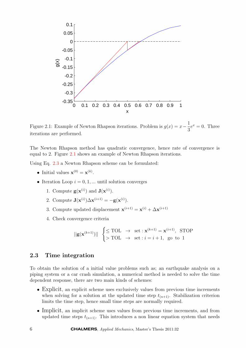
Figure 2.1: Example of Newton Rhapson iterations. Problem is g(x) = x− 1
3ex = 0. Three
iterations are performed.
The Newton Rhapson method has quadratic convergence, hence rate of convergence isequal to 2. Figure 2.1 shows an example of Newton Rhapson iterations.
Using Eq. 2.3 a Newton Rhapson scheme can be formulated:
• Initial values x(0) = x(k).
• Iteration Loop i = 0, 1, ... until solution converges
1. Compute g(x(i)) and J(x(i)).
2. Compute J(x(i))∆x(i+1) = −g(x(i)).
3. Compute updated displacement x(i+1) = x(i) + ∆x(i+1)
4. Check convergence criteria
||g(x(k+1))||
{≤ TOL → set : x(k+1) = x(i+1), STOP
> TOL → set : i = i+ 1, go to 1
2.3 Time integration
To obtain the solution of a initial value problems such as; an earthquake analysis on apiping system or a car crash simulation, a numerical method is needed to solve the timedependent response, there are two main kinds of schemes:
• Explicit, an explicit scheme uses exclusively values from previous time incrementswhen solving for a solution at the updated time step t(n+1). Stabilization criterionlimits the time step, hence small time steps are normally required.
• Implicit, an implicit scheme uses values from previous time increments, and fromupdated time steps t(n+1). This introduces a non linear equation system that needs
6 , Applied Mechanics, Master’s Thesis 2011:32

to be solved at each time step, for example, by using a Newton Rhapson method, seeSection 2.2. Implicit schemes are unconditionally stable.
Both methods are frequently used to solve time dependent problems, the nature of thestudied problem determines which method that are best suited.
2.3.1 Newmark method
A widely used scheme is the Newmark method. The presentation of the scheme followsthe contents in [17]. Approximations on updated displacement, un+1, and velocity, vn+1,at time tn+1 are the base of the method,
un+1 = un + ∆tvn +(∆t)2
2[(1− 2β)an + 2βan+1]
vn+1 = vn + ∆t[(1− λ)an + λan+1](2.4)
where β and λ are parameters that controls the convergence, stability and accuracy ofthe solution. Depending on how those parameters are chosen the Newmark method canbe either explicit and implicit. As previously mentioned, an implicit scheme uses bothknown quantities from previous times and quantities from updated times tn+1, by choosingβ = 1/4 and λ = 1/2 the scheme is implicit.
According to a mathematical analysis, [7], of the Newmark method, limiting inequalitieson β and λ were established as
0 ≤ β ≤ 0.5
0 ≤ λ ≤ 1.
By using approximate values on un+1 and vn+1 and introducing those into the spatialdiscretized form of the equations of motion and solving with, for example, the NewtonRhapson method, the unknown accelerations an+1 can be determined. Then Eq. 2.4 andan+1 yield the unknown displacements and velocities at time tn+1.
2.4 Gap Modeling
A boundary value problem that involves contact occurs frequently in almost all scientificdisciplines. Due to the characteristics of a contact problem it is highly nonlinear andhence demands large computer resources. Historically contact mechanics problems wereoften approximated by special assumptions, or special design codes that compensates forcontacts for each case, for example, in ASME [5], but the improvements within the com-puter technology allow todays engineers to numerically solve contact problems using bothimplicit and explicit finite element analyses.
Contact boundary value problems can be divided into two general groups, rigid-to-flexibleand flexible-to-flexible. A general formulation of a one dimensional case of rigid to flexiblecontact is presented below and follows [16].
2.4.1 General formulation
Consider the static frictionless contact problem consisting of a point mass m and a springwith stiffness k that supports a mass. The point mass experiences a gravitational load and
, Applied Mechanics, Master’s Thesis 2011:32 7
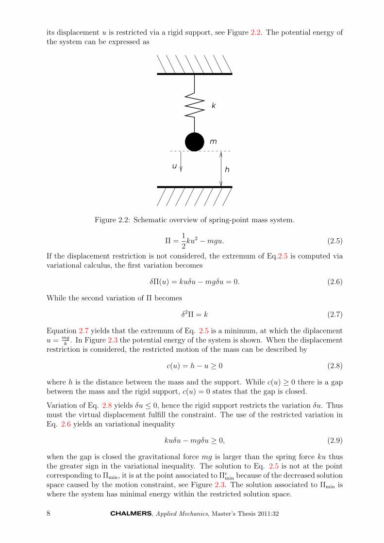
its displacement u is restricted via a rigid support, see Figure 2.2. The potential energy ofthe system can be expressed as
hu
m
k
Figure 2.2: Schematic overview of spring-point mass system.
Π =1
2ku2 −mgu. (2.5)
If the displacement restriction is not considered, the extremum of Eq.2.5 is computed viavariational calculus, the first variation becomes
δΠ(u) = kuδu−mgδu = 0. (2.6)
While the second variation of Π becomes
δ2Π = k (2.7)
Equation 2.7 yields that the extremum of Eq. 2.5 is a minimum, at which the diplacementu = mg
k. In Figure 2.3 the potential energy of the system is shown. When the displacement
restriction is considered, the restricted motion of the mass can be described by
c(u) = h− u ≥ 0 (2.8)
where h is the distance between the mass and the support. While c(u) ≥ 0 there is a gapbetween the mass and the rigid support, c(u) = 0 states that the gap is closed.
Variation of Eq. 2.8 yields δu ≤ 0, hence the rigid support restricts the variation δu. Thusmust the virtual displacement fulfill the constraint. The use of the restricted variation inEq. 2.6 yields an variational inequality
kuδu−mgδu ≥ 0, (2.9)
when the gap is closed the gravitational force mg is larger than the spring force ku thusthe greater sign in the variational inequality. The solution to Eq. 2.5 is not at the pointcorresponding to Πmin, it is at the point associated to Πc
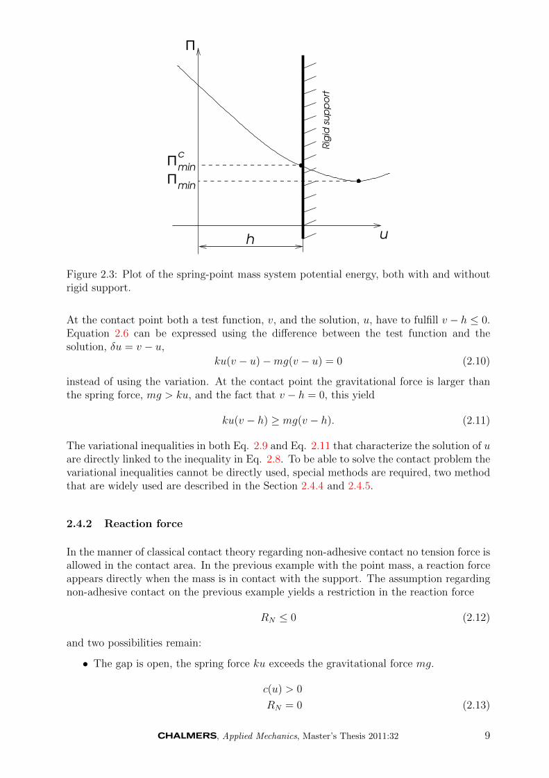
min because of the decreased solutionspace caused by the motion constraint, see Figure 2.3. The solution associated to Πmin iswhere the system has minimal energy within the restricted solution space.
8 , Applied Mechanics, Master’s Thesis 2011:32
Π
uh
Πmin
minΠc
Rig
id s
up
po
rt
Figure 2.3: Plot of the spring-point mass system potential energy, both with and withoutrigid support.
At the contact point both a test function, v, and the solution, u, have to fulfill v − h ≤ 0.Equation 2.6 can be expressed using the difference between the test function and thesolution, δu = v − u,
ku(v − u)−mg(v − u) = 0 (2.10)
instead of using the variation. At the contact point the gravitational force is larger thanthe spring force, mg > ku, and the fact that v − h = 0, this yield
ku(v − h) ≥ mg(v − h). (2.11)
The variational inequalities in both Eq. 2.9 and Eq. 2.11 that characterize the solution of uare directly linked to the inequality in Eq. 2.8. To be able to solve the contact problem thevariational inequalities cannot be directly used, special methods are required, two methodthat are widely used are described in the Section 2.4.4 and 2.4.5.
2.4.2 Reaction force
In the manner of classical contact theory regarding non-adhesive contact no tension force isallowed in the contact area. In the previous example with the point mass, a reaction forceappears directly when the mass is in contact with the support. The assumption regardingnon-adhesive contact on the previous example yields a restriction in the reaction force
RN ≤ 0 (2.12)
and two possibilities remain:
• The gap is open, the spring force ku exceeds the gravitational force mg.
c(u) > 0
RN = 0 (2.13)
, Applied Mechanics, Master’s Thesis 2011:32 9

• The gap is closed, the point mass is in contact with the rigid support.
c(u) = 0
RN < 0 (2.14)
If the two cases are combined they can form the statement
c(u) ≥ 0
RN ≤ 0 (2.15)
RNc(u) = 0
known as a Hertz-Signorini-Moreau condition. In Figure 2.4 the gap size, Equation 2.8,is plotted versus the reaction force. One point of the curve is not differentiable, thusnon-smooth mathematical methods are to be applied.
c(u)
RN
Figure 2.4: Plot of reaction force versus c(u) = h− u.
2.4.3 Friction
If the gap is assumed to be closed, the point mass is in contact with the rigid support thusRN < 0. In the case of friction, a external force, FT , is added in the tangential directionto the rigid supports plane. Free body diagram is shown in Figure 2.5 and equilibriumequations for the system. A simple friction model, Coulomb’s law, is adopted to describefriction in the contact between the point mass and the support. Two states exist: stickand slip. Stick allows no motion between the mass and the support, while a certain relativemotion between the support and the mass, uT, is allowed when slip occurs. This yieldsthree different cases:
1. Coulomb’s law yields an inequality
f(RN, RT) = |RT|+ µRN ≤ 0. (2.16)
Where µ is the friction coefficient. This relationship can now be used to separatebetween stick and slip.
10 , Applied Mechanics, Master’s Thesis 2011:32

k
m
F T F T
mg
R T
RN
kh
Figure 2.5: Free body diagram of spring-point mass system.
2. When stick occurs|RT| < −µRN, (2.17)
hence no motion between the mass and the support, uT = 0. Yields the reactionforce RT.
3. Finally slip occurs when|RT| = −µRN, (2.18)
hence relative motion between mass and spring, uT 6= 0. RT can be established fromEq. 2.18.
Also as for Eq. 2.15 these equations forms a Kuhn-Tucker condition.
|uT | ≥ 0
f ≤ 0 (2.19)
f |uT | = 0
In Figure 2.6 a relationship between RT and uT is plotted. As for 2.4 non differentiablepoints in the plot of force versus deflection exist, which cause mathematical difficulties.
, Applied Mechanics, Master’s Thesis 2011:32 11

u T
R T
Figure 2.6: Tangential force against displacement.
2.4.4 Lagrange Multiplier Method
One method to obtain a solution to a contact problem that is constrained by an inequalityEq. 2.8, is the Lagrange Multiplier. According to [16], assume that the contact is active,hence the conditions in Eq. 2.14 is fulfilled. In that case the Lagrange Multiplier methodcontributes with a term to the systems potential energy, Eq. 2.5. The term contains themotion constraint.
Π(u, λ) =1
2ku2 −mgu+ λc(u) (2.20)
From Eqs. 2.20 and 2.15 one can conclude that the reaction force R are equivalent to λ.By variation of Equation 2.20, δu and δλ can be varied independently, two equations areestablished, namely
kuδu−mgδu− λδu = 0 (2.21)
δλc(u) = 0 (2.22)
The equilibrium equation of the mass with the contribution from the reaction force whenthe mass is in contact with the rigid support are stated in Eq. 2.21, and the second equationof the two above represents the fulfillment of the motion constraint, Eq. 2.8, see Figure2.7 . Hence the previous restriction on the variation no longer applies, and it is possible tosolve for λ thus also for RN
λ = kh−mg = RN . (2.23)
12 , Applied Mechanics, Master’s Thesis 2011:32

hu
m
k
λ
Figure 2.7: Schematic overview of spring-point mass system with Lagrange multiplier.
2.4.5 Penalty Method
Another method widely used to solve contact problems in finite element analysis is thePenalty method. When the constraint is active, the point mass is in contact with the rigidsupport and a penalty term is added to the energy in Eq. 2.5, which yields
Π =1
2ku2 −mgu+
1
2ε[c(u)]2 with ε > 0 (2.24)
A comparison between the additional energy penalty term in Eq. 2.24 and the energy ofa simple spring shows that their structure are equal, hence ε can be construed as a springstiffness on a spring in the contact between the mass and the rigid support, see Figure 2.8.Variation of Equation 2.24 in the case of contact yields
kuδu−mgδu− εc(u)δu = 0 (2.25)
and the solution u then becomes
u =(mg + εh)
k + ε(2.26)
and the corresponding motion constraint equation reads
c(u) = h− u =kh−mgk + ε
(2.27)
When contact occurs mg ≥ kh, and according to the constraint Equation 2.27 the mass willpenetrate into the rigid support. This is physically equal to compression of the spring inthe contact, see Figure 2.8. Two limiting cases can be determined in the Penalty method,since the gap Eq. 2.27 is only fulfilled in the limit ε→∞⇒ c(u)→ 0:
1. ε → ∞ ⇒ u − h → 0, hence for large values on ε the spring stiffness is large, hencesmall penetration occurs and the right solution, u, is approaching.
2. ε→ 0 is valid when there is no contact, hence inactive constraints. If contact occurswhen ε is small a solution with large penetration would occur.
Using Eq. 2.25 the reaction force is obtained,
RN = εc(u) = {in this case} =ε
k + ε(kh−mg). (2.28)
When ε → 0 Eq. 2.28 yields the same solution as with the Lagrange multiplier methodEq. 2.23.
, Applied Mechanics, Master’s Thesis 2011:32 13

hu
m
k
ε
Figure 2.8: Spring-point mass system, with and without additional penalty spring.
2.5 Damping
For all structural dynamic analyses, an equation of motion is formulated. The linearspatially discretized equation of motion under externally applied time dependent forcescan be written as
Mu(t) + Cu(t) + Ku(t) = F(t) (2.29)
where M is the mass matrix, C is the damping matrix, K is the stiffness matrix and F(t) isthe external load vector. In this section two examples of damping will be discussed, morespecifically; Rayleigh damping and constant damping.
The modeling of damping of large systems is usually quite complicated. The knowledgeabout how to model damping for a multiple degree of freedom system is limited and oftenthe most effective way is to describe it as Rayleigh damping. It is assumed that thedamping matrix is proportional to a combination of the mass and stiffness matrices in thefollowing manner
C = αM + βK (2.30)
where α and β are predefined constants. An orthogonal transform using the undampedmodes of this damping matrix leads to the following expression
2ζωi = α + βω2i (2.31)
where ωi is the eigenfrequency and ζ is the damping ratio. The latter can be rewritten as
ζ =α
2ωi
+βωi
2(2.32)
ζ=1 means critical damping. Unlike constant damping, Rayleigh damping varies withfrequency. The α and β constants are usually determined so that the damping curvematch two damping values. These values do often belong to the lowest and highest eigenfrequencies of interest, or measured values. For example shown in Figure 2.9 is a constantdamping of 5% as well as the two different parts of 2.32. Its clear that the α-part (mass
14 , Applied Mechanics, Master’s Thesis 2011:32
0 2 4 6 8 10 12 14 16 180
0.02
0.04
0.06
0.08
0.1
0.12
Frequency - ω [Hz]
Dam
ping
ratio
n - ζ
Rayleigh dampingα-dampingβ-dampingConstant damping
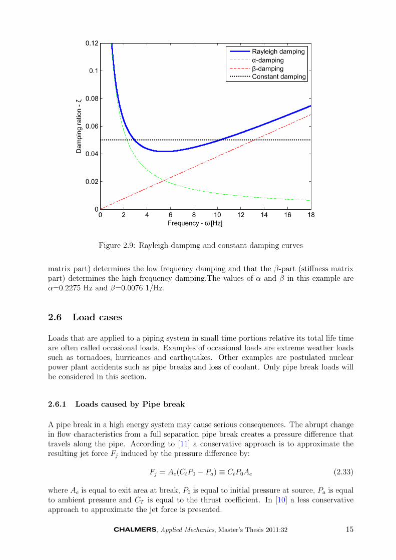
Figure 2.9: Rayleigh damping and constant damping curves
matrix part) determines the low frequency damping and that the β-part (stiffness matrixpart) determines the high frequency damping.The values of α and β in this example areα=0.2275 Hz and β=0.0076 1/Hz.
2.6 Load cases
Loads that are applied to a piping system in small time portions relative its total life timeare often called occasional loads. Examples of occasional loads are extreme weather loadssuch as tornadoes, hurricanes and earthquakes. Other examples are postulated nuclearpower plant accidents such as pipe breaks and loss of coolant. Only pipe break loads willbe considered in this section.
2.6.1 Loads caused by Pipe break
A pipe break in a high energy system may cause serious consequences. The abrupt changein flow characteristics from a full separation pipe break creates a pressure difference thattravels along the pipe. According to [11] a conservative approach is to approximate theresulting jet force Fj induced by the pressure difference by:
Fj = Ae(CtP0 − Pa) ≡ CtP0Ae (2.33)
where Ae is equal to exit area at break, P0 is equal to initial pressure at source, Pa is equalto ambient pressure and CT is equal to the thrust coefficient. In [10] a less conservativeapproach to approximate the jet force is presented.
, Applied Mechanics, Master’s Thesis 2011:32 15

Figure 2.10 shows a schematic overview of the steam piping system that has been subjectedto a pipe break, while Figure 2.11 shows the resulting force components versus time.
F2
F3
F1
Break
Tank
Figure 2.10: Schematic view of pipe system after pipe break.
Figure 2.11: Force components from schematic pipe subjected to a pipe break. Breakoccurs at time=0.
16 , Applied Mechanics, Master’s Thesis 2011:32

3 Method
The approach for this thesis was to study both a typical piping system, TPS, (from a typicalpower plant) and a simplified piping system, SPS. In Section 3.1 and 3.2 the systems aredescribed thoroughly. ANSYS was mainly used for the piping analysis. As mentioned insection 1.1 Pipestress is commonly used in the Swedish nuclear industry. Due to this, theANSYS finite element model was verified against a Pipestress finite element model.
3.1 Simplified piping system
This system is constructed to resemble a steam system that is ranging between a pressurecontrol tank and the main steam system, see Figure 3.1. The pipe system is subjected toa pipe break load, see Section 2.6.
Tank
Support B
Support A
Break
Figure 3.1: Simplified piping systems, geom1.
3.1.1 Geometry and Material data for the simplified system
One base geometry was created, geom1, see Figure 3.1. Geom1 consists of three bends, twosupports (one vertical and one horizontal) and two anchor points. One of the geometryparameters was then alternated in four steps in the base geometry which created fourversions of geom1, see Table 3.1.1 and Figure 3.2 for dimensions and cross sectional data.All supports except the anchor points are structural steel supports, with a gap,c, betweenthe pipe and the support see Figure 3.4. The material used for the pipe in the analysiswas SA155 Gr C55, see Table 3.1.1 for material properties, which is a typical steel usedfor high pressure service, see [6] for further information regarding material.
, Applied Mechanics, Master’s Thesis 2011:32 17

Figure 3.2: Simplified piping systems, geom1.
Table 3.1: Geometrical data and material data for geom1
h1 [m] h2 [m] l1 [m] l2 [m] l3 [m] R1 [m]
geom1 v1 13 13 16.5 16.5 16.5 1geom1 v2 15 13 16.5 16.5 16.5 1geom1 v3 17 13 16.5 16.5 16.5 1geom1 v4 19 13 16.5 16.5 16.5 1
Rinner [m] Router [m]
geom1 0.365 0.381
E [Pa] ν [ ] ρ [ kgm3 ]
geom1 195e9 0.3 7850
18 , Applied Mechanics, Master’s Thesis 2011:32

3.1.2 Finite element model for the simplified system
A finite element model of the piping system was modeled in ANSYS with the linear elasticelements pipe16 and pipe18, Figure 3.3 displays the calculation domain. See [2] for moreinformation regarding the elements used to model the pipe. The supports were modeledin two manners, one with combin14 spring elements and the other one was modeled withconta178 contact element and combin14 spring elements connected in series, see Figure 3.4.The lagrange multiplier method was used in the contact surface normal-direction and thePenalty method was used in contact surface tangential-(frictional) direction, see Section2.4.
Figure 3.3: Calculation domain for geom1.v1.
COMBIN14
k
COMBIN14
k
c
CONTA178
c
CONTA178
COMBIN14
k
Figure 3.4: Schematic figure over a support modeled with conta178 and combin14 elementsto the left and a support modeled with combin14 to the right.
, Applied Mechanics, Master’s Thesis 2011:32 19
3.1.3 Analysis of the simplified system
Here we present the settings that are similar in all of the various analyses that wereconducted for the SPS. All analyses hereinafter defined for the SPS are implicit finiteelement analyses with time history loading that are performed in ANSYS.
Load
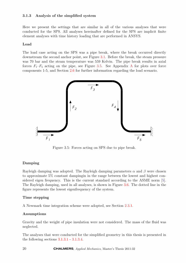
The load case acting on the SPS was a pipe break, where the break occurred directlydownstream the second anchor point, see Figure 3.1. Before the break, the steam pressurewas 70 bar and the steam temperature was 559 Kelvin. The pipe break results in axialforces F1–F5 acting on the pipe, see Figure 3.5. See Appendix A for plots over forcecomponents 1-5, and Section 2.6 for further information regarding the load scenario.
F1
F4F
2
F3
F5
Figure 3.5: Forces acting on SPS due to pipe break.
Damping
Rayleigh damping was adopted. The Rayleigh damping parameters α and β were chosento approximate 5% constant dampingin in the range between the lowest and highest con-sidered eigen frequency. This is the current standard according to the ASME norm [5].The Rayleigh damping, used in all analyses, is shown in Figure 3.6. The dotted line in thefigure represents the lowest eigenfrequency of the system.
Time stepping
A Newmark time integration scheme were adopted, see Section 2.3.1.
Assumptions
Gravity and the weight of pipe insulation were not considered. The mass of the fluid wasneglected.
The analyses that were conducted for the simplified geometry in this thesis is presented inthe following sections 3.1.3.1 - 3.1.3.4.
20 , Applied Mechanics, Master’s Thesis 2011:32

0 2 4 6 8 100
0.1
0.2
0.3
0.4
0.5
0.6
0.7
0.8
Frequency [Hz]
ζ [ ]
5% constant dampingRayleig dampingω1,geom1_v1 = 1.79 Hz
Figure 3.6: Rayleigh curve α = 1.5814 Hz, β = 0.0015093 1/Hz and ω1,geom1 is the lowesteigenfrequency of the system.
3.1.3.1 Time step evaluation
When the piping system is subjected to a time history pipe break load, the gaps betweenthe supports and the pipe will occasionally be closed. Hence the pipe will experience highdecelerations and due to this high amplitude short duration impact forces arise in thecontact between the pipe and the supports.
To be able to resolve those short duration forces sufficiently small time steps were needed.In the time step evaluation analysis, the time steps were incrementally lowered accordingto
timestep(i) = 0.001
(2
3
)(i−1)
[s] (3.1)
where i is the current increment. The time step size was lowered until both maximumcontact force and maximum pipe stress converged.
The gap size used in the analysis corresponds to the case where highest stresses in thepipe occur and impact between the pipe and the supports takes place at least two times.Both support A and B had the equal initial gap size. Geom1 version one was used in theanalysis.
3.1.3.2 Contact surface friction
The influence of friction in the contact was investigated on the simplified piping system.As mentioned in Section 3.1.2, when friction is considered the Penalty method is used in
, Applied Mechanics, Master’s Thesis 2011:32 21

the contact planes tangential directions with µ as the friction coefficient, combined withLagrange multiplier method in the contact planes normal directions, see Section 2.4.5.
The gap sizes were chosen so that support A experienced maximum deformation in thecontact normal direction. Three different gap sizes were analyzed each of them correspond-ing to an local maximum point in a ”max support deformation versus gap size” plot. Bothsupport A and B had equal initial gap size in the three simulations performed. Geom1version one were used in the analysis.
3.1.3.3 Support stiffness
The occurrence of support reaction force impulses made it very interesting to examine theinfluence of the modeled support stiffness, both for a support with and without gaps. Thepurpose was to lower the stiffness and therefor also lower the deceleration of the pipe hittingthe support. This should in theory eliminate the reaction force spikes. The first version ofthe simplified piping system was chosen, see Section 3.1.1, and the supports were modeledwith a 25.7mm gap. Previous analyses of this system, with standard support stiffness of700kN/mm, showed that this gap size gave rise to the highest pipe stresses. The systemwith and without a gap was then analyzed with twenty different support stiffnesses, withthe largest one being the standard stiffness, according to the formula following
k(i) = 18.2588(1.2i) [kN/mm] (3.2)
i = 1 : 20
In Figure 3.7 the stiffness k(i) versus increments, i is plotted. It was also interesting toinvestigate if one could approximate the behavior of a gap support by varying the stiffnessof support without a gap. To see the effects of this clearly, the extreme values 700kN/mmand 21.9kN/mm were compared. Booth the reaction force of support A and the stress ofthe adjacent element were investigated.
3.1.3.4 Gap size
In this analysis the four different versions of geom1 were analyzed,v1− v4, see Table 3.1.1.A gap, c, existed between the pipe and its supports and the influence of the size of thisgap was studied. The gap size was incrementally changed in 43 steps for each of the fourgeometries, according to:
c(i) = 0.0001(i− 1)2.41 [m] (3.3)
were i is the current increment numbers and changes according to
i = 1 : 43.
The curve that represents the initial gap size is displayed in Figure 3.8. The gaps wereequally changed in both support A and B. Friction in the contact between the supportsand the pipe was neglected.
22 , Applied Mechanics, Master’s Thesis 2011:32

0 5 10 15 200
100
200
300
400
500
600
700
i
Supp
ort s
tiffn
ess
[kN
/mm
]
Figure 3.7: Stiffness versus increments.
0 5 10 15 20 25 30 35 40 450
0.1
0.2
0.3
0.4
0.5
0.6
0.7
0.8
0.9
i
Gap
siz
e [m
]
Figure 3.8: Initial gap size versus increments.
, Applied Mechanics, Master’s Thesis 2011:32 23

3.2 Typical piping system
This system is a typical main steam system that is ranging form the steam generator untilthe containment wall. Then the system continuous through the containment wall towardsthe turbine. In this thesis the part of the system that is inside the containment was analyzedduring a typical pipe break further downstream on the outside of the containment. Thepiping system belongs to ASME safety class 1 and the load scenario is level D.
Figure 3.9: Typical piping system with anchors and supports.
3.2.1 Geometry and Material data for the typical piping system
The analyzed part of the TPS contains of two anchor points and four pipe supports seeFigure 3.9. The first anchor point is situated where the pipe is connected to the steamgenerator and the second one is situated where the pipe reaches the containment wall.The supports are of rigid restraint type, see Section 1.1 hence a rigid frame built up byconstruction steel and there exists a gap between the pipe and the support. Material isSA155 Gr C55 which is a typical steel used for high pressure service, see [6].
The dimensions of the piping system are displayed in Figure 3.9, cross section data andmaterial data are stated in Table 3.2.1.
3.2.2 Finite element model of the typical piping system
A finite element model of the system was created in ANSYS. The pipe was modeled withlinear elastic elements pipe16 and pipe18, see ANSYS manual, [2], for more informationregarding the elements. Figure 3.10 displays the calculation domain. The rigid restraintsupports were modeled with conta178 and combin14 elements see Figure 3.4. Conta178 is
24 , Applied Mechanics, Master’s Thesis 2011:32

Table 3.2: Geometrical data and material data for TPS
L1 [m] L2 [m] L3 [m] L4 [m] L5 [m] L6 [m] L7 [m]
19.5 4 1.4142 5 4.5 10 12
R1 [m] R2 [m] R3 [m] R4 [m] R5 [m] R6 [m]
1.14 1.14 1.14 15 0.85 1.14
Rinner [m] Router [m]
0.365 0.381
E [Pa] ν [ ] ρ [ kgm3 ]
195e9 0.3 7850
a node-to-node contact element, that can use both the Lagrange multiplier method andthe Penalty method to model the gap. Lagrange multiplier method was used in this caseand friction was neglected. At penetration of the containment wall and at the connectionto the steam generator all degrees of freedom were fixed in the finite element model.
Figure 3.10: Finite element model of TPS.
3.2.3 Analysis of the typical piping system
In the analysis the gap size, c, was equally incrementally changed in all supports, accordingto
c(i) =0.042
49(i− 1) [m] (3.4)
where i is the current increment numbers and changes according to
i = 1 : 50.
, Applied Mechanics, Master’s Thesis 2011:32 25

In Figure 3.11 the curve that represents the initial gap size is plotted.
0 10 20 30 40 500
0.005
0.01
0.015
0.02
0.025
0.03
0.035
0.04
0.045
i
Gap
siz
e [m
]
Figure 3.11: Initial gap size versus increments.
Load
The load case acting on the TPS was a pipe break where the break occurred downstreamthe second anchor point, hence outside the containment wall, see Figure 3.9. The pipebreak results in axial forces F1–F9 acting on the pipe, see Figure 3.12. See appendix Bfor plots and tables over force components 1-9, and Section 2.6 for further informationregarding the load scenario.
Damping
Equal damping properties as for the SPS.
Time stepping
Equal time stepping scheme as for the SPS.
Assumptions Same assumptions as for the SPS, except that friction between the pipeand its supports always were neglected.
3.3 Validation
In the Swedish nuclear industry, the pipe analysis program Pipestress is widely used. To beable to interpret and compare the results from ANSYS analyses with Pipestress analyses,the dynamic properties of the ANSYS finite element models 3.1.2 and 3.2.2, without thecontact elements conta178, are verified against Pipestress models of the same systems.
The verification covers:
26 , Applied Mechanics, Master’s Thesis 2011:32

Figure 3.12: Forces acting on TPS due to pipe break.
1. Total mass for the models
2. Eigenfrequencies and eigen modes
3. Dead weight analysis
4. Results from pipe break analysis.
, Applied Mechanics, Master’s Thesis 2011:32 27

28 , Applied Mechanics, Master’s Thesis 2011:32
4 Results
This section is divided into two subsections, one for the simplified geometry and one for thetypical piping system, see Section 3.1 and 3.2 for information about the piping systems.
4.1 Simplified piping system
Here, the results from the analysis of the simplified piping system are presented. Thesection is divided into five subsections, Time step evaluation, Contact surface friction,Support stiffness, Gap size and Stiffness approximation.
4.1.1 Time step evaluation
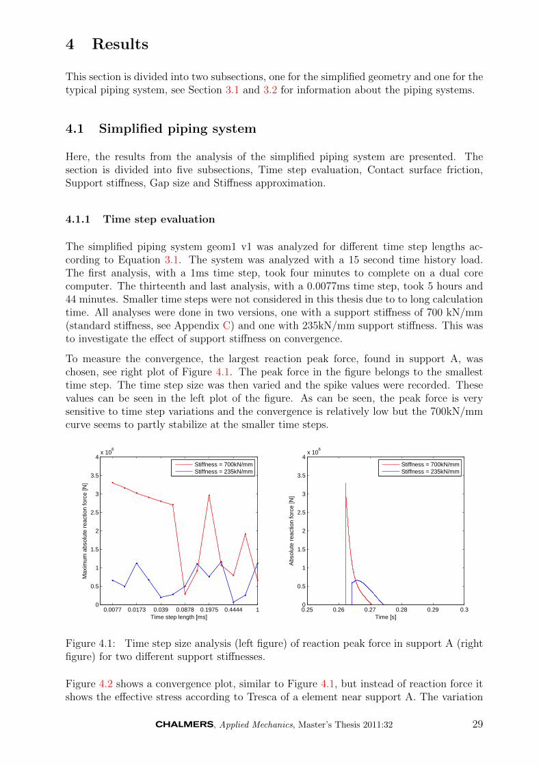
The simplified piping system geom1 v1 was analyzed for different time step lengths ac-cording to Equation 3.1. The system was analyzed with a 15 second time history load.The first analysis, with a 1ms time step, took four minutes to complete on a dual corecomputer. The thirteenth and last analysis, with a 0.0077ms time step, took 5 hours and44 minutes. Smaller time steps were not considered in this thesis due to to long calculationtime. All analyses were done in two versions, one with a support stiffness of 700 kN/mm(standard stiffness, see Appendix C) and one with 235kN/mm support stiffness. This wasto investigate the effect of support stiffness on convergence.
To measure the convergence, the largest reaction peak force, found in support A, waschosen, see right plot of Figure 4.1. The peak force in the figure belongs to the smallesttime step. The time step size was then varied and the spike values were recorded. Thesevalues can be seen in the left plot of the figure. As can be seen, the peak force is verysensitive to time step variations and the convergence is relatively low but the 700kN/mmcurve seems to partly stabilize at the smaller time steps.
0.0077 0.0173 0.039 0.0878 0.1975 0.4444 10
0.5
1
1.5
2
2.5
3
3.5
4x 10
6
Time step length [ms]
Max
imum
abs
olut
e re
actio
n fo
rce
[N]
0.25 0.26 0.27 0.28 0.29 0.30
0.5
1
1.5
2
2.5
3
3.5
4x 10
6
Time [s]
Abs
olut
e re
actio
n fo
rce
[N]
Stiffness = 700kN/mmStiffness = 235kN/mm
Stiffness = 700kN/mmStiffness = 235kN/mm
Figure 4.1: Time step size analysis (left figure) of reaction peak force in support A (rightfigure) for two different support stiffnesses.
Figure 4.2 shows a convergence plot, similar to Figure 4.1, but instead of reaction force itshows the effective stress according to Tresca of a element near support A. The variation
, Applied Mechanics, Master’s Thesis 2011:32 29

with time step size is very small and it converges much better than the correspondingreaction force.
0.0077 0.0173 0.039 0.0878 0.1975 0.4444 13.6
3.8
4
4.2
4.4
4.6
4.8x 10⁷
Time step length [ms]
Max
imum
stre
ss [P
a]
0.08 0.1 0.12 0.14 0.16 0.18 0.2 0.220
0.5
1
1.5
2
2.5
3
3.5
4
4.5x 10⁷
Time [s]
Stre
ss [P
a]
Stiffness = 700kN/mmStiffness = 235kN/mm
Stiffness = 700kN/mmStiffness = 235kN/mm
Figure 4.2: Time step size analysis (left figure) of stress intensity in pipe element closestto support A (right figure).
Figure 4.3 shows the same thing as Figure 4.2 but for the element located close to supportB. This is the element that experiences the largest stress. This stress is relatively slow andthe convergence is therefore very good.
0.0077 0.0173 0.039 0.0878 0.1975 0.4444 16.78
6.8
6.82
6.84
6.86
6.88
6.9
6.92
6.94
x 107
Time step length [ms]
Max
imum
stre
ss [P
a]
0.1 0.15 0.2 0.25 0.3 0.35 0.4 0.450
1
2
3
4
5
6
7
x 107
Time [s]
stre
ss [P
a]
Stiffness = 700kN/mmStiffness = 235kN/mm
Stiffness = 700kN/mmStiffness = 235kN/mm
Figure 4.3: Time step size analysis (left figure) of stress according to Tresca in pipe elementclosest to support B (right figure).
4.1.2 Contact surface friction
As described in Section 3.1.3.2, analyses with friction in the contact surface between thesupport and the pipe were conducted. The purpose with these analyses were to investigatethe influence on the piping system and its supports when friction in the contact surfacebetween the pipe and supports was accounted for. Three different gap sizes were chosen,namely, 15.01 mm, 68.29 mm and 257.1 mm. The selection of those gap sizes was based
30 , Applied Mechanics, Master’s Thesis 2011:32

on maximum support deformation. Hence each of the selected cases corresponds to a localmaximum in support deformation in the contact normal direction during a pipe break loadcase, see Figure 4.4.
0 0.1 0.2 0.3 0.4 0.5 0.6 0.7 0.8 0.90
0.2
0.4
0.6
0.8
1
1.2
1.4
1.6
1.8x 10
−3
Gap size [m]
Max
sup
port
def
orm
atio
n [m
]
Support A in positive z−dirSupport A in negative z−dirInvestigated cases
Figure 4.4: Max support deformation in the normal-direction plotted versus gap size,selected cases for friction analysis.
The contact was modeled using the Lagrange multiplier method in the contact normal-direction and the Penalty method in the contact tangential (friction)-direction.
The stresses in the piping system were generally equal or slightly lower when friction wastaken into account. Maximum stress in the pipe occurred at the same location, both withand without friction in the contact surfaces. See Figure 4.5-4.7 for plots over stress versustime in the elements close to supports A and B for the three different cases.
, Applied Mechanics, Master’s Thesis 2011:32 31

0 0.5 1 1.5 20
1
2
3
4
5
x 107
Time [s]
Stre
ss [P
a]
Support A - Gap = 15 mm
No frictionFriction, µ = 0.18
0 0.5 1 1.5 20
1
2
3
4
5
x 107
Time [s]
Stre
ss [P
a]
Support B - Gap = 15 mm
No frictionFriction, µ = 0.18
Figure 4.5: Stress versus time in pipe elements close to supports A and B, with and withoutfriction, gap = 15 mm.
0 0.5 1 1.5 20
0.5
1
1.5
2
2.5
3
3.5
4
4.5
5x 10⁷
Time [s]
Stre
ss [P
a]
Support A - Gap = 68.3 mm
No frictionFriction, µ = 0.18
0 0.5 1 1.5 20
0.5
1
1.5
2
2.5
3
3.5
4
4.5x 10⁷
Time [s]
Stre
ss [P
a]
Support B - Gap = 68.3 mm
No frictionFriction, µ = 0.18
Figure 4.6: Stress versus time in pipe elements close to supports A and B, with and withoutfriction, gap = 68 mm.
32 , Applied Mechanics, Master’s Thesis 2011:32

0 0.5 1 1.5 20
1
2
3
4
5
x 107
Time [s]
Stre
ss [P
a]
Support A - Gap = 257 mm
No frictionFriction, µ = 0.18
0 0.5 1 1.5 20
5
10
15
x 106
Time [s]
Stre
ss P
a]
Support B - Gap = 257 mm
No frictionFriction, µ = 0.18
Figure 4.7: Stress versus time in pipe elements next to support A and B, with and withoutfriction, gap = 257 mm.
In Figure 4.8 -4.10, the reaction forces of the two supports are shown. Reaction forcesnormal to the contact plane and in the case when friction is accounted for also additionaltangential forces are plotted.
0 0.5 1 1.5 2
-1.5
-1
-0.5
0
0.5
1
1.5
x 106
Time [s]
Rea
ctio
norc
e [N
]
Support A - Gap = 15 mm
No friction, normal-dirFriction, normal-dir, µ = 0.18Friction, tangential-dir, µ = 0.18
0 0.5 1 1.5 2
-1.5
-1
-0.5
0
0.5
1
1.5
x 106
Time [s]
Rea
ctio
norc
e [N
]
Support B - Gap = 15 mm
No friction, normal-dirFriction, normal-dir, µ = 0.18Friction, tangential-dir, µ = 0.18
Figure 4.8: Force versus time in pipe elements next to support A and B, with and withoutfriction, gap = 15 mm.
Generally slightly higher support reaction forces were obtained in the case was no frictionon the contact surface were assumed.
, Applied Mechanics, Master’s Thesis 2011:32 33

0 0.5 1 1.5 2
0
0.5
1
1.5
2
2.5
3
x 106
Time [s]
Rea
ctio
norc
e [N
]
Support A - Gap = 68 mm
No friction, normal-dirFriction, normal-dir, µ = 0.18Friction, tangential-dir, µ = 0.18
0 0.5 1 1.5 2
0
0.5
1
1.5
2
2.5
3
x 106
Time [s]
Rea
ctio
norc
e [N
]
Support B - Gap = 68 mm
No friction, normal-dirFriction, normal-dir, µ = 0.18Friction, tangential-dir, µ = 0.18
Figure 4.9: Force versus time in pipe elements next to support A and B, with and withoutfriction, gap = 68 mm.
0 0.5 1 1.5 2
-6
-4
-2
0
2
4
6
8x 10
5
Time [s]
Rea
ctio
norc
e [N
]
Support A - Gap = 257 mm
No friction, normal-dirFriction, normal-dir, µ = 0.18Friction, tangential-dir, µ = 0.18
0 0.5 1 1.5 2
-6
-4
-2
0
2
4
6
8x 10
5
Time [s]
Rea
ctio
norc
e [N
]
Support B - Gap = 257 mm
No friction, normal-dirFriction, normal-dir, µ = 0.18Friction, tangential-dir, µ = 0.18
Figure 4.10: Force versus time in pipe elements next to support A and B, with and withoutfriction, gap = 257 mm.
34 , Applied Mechanics, Master’s Thesis 2011:32

In Figure 4.11-4.13 the time history of the displacement in normal and tangential directionof the pipe nodes located next to the supports A and B is plotted, for the three differentcases.
0 0.5 1 1.5 2
-0.15
-0.1
-0.05
0
0.05
0.1
Time [s]
Dis
plac
emen
t [m
]
Support A - Gap = 15 mm
No friction, normal-dirFriction, normal-dir, µ = 0.18No friction, tangetial-dirFriction, tangential-dir, µ = 0.18
0 0.5 1 1.5 2
-0.25
-0.2
-0.15
-0.1
-0.05
0
0.05
0.1
0.15
Time [s]
Dis
plac
emen
t [m
]
Support B - Gap = 15 mm
No friction, normal-dirFriction, normal-dir, µ = 0.18No friction, tangetial-dirFriction, tangential-dir, µ = 0.18
Figure 4.11: Displacement versus time in pipe elements next to support A and B, withand without friction, gap = 15 mm.
0 0.5 1 1.5 2
-0.2
-0.15
-0.1
-0.05
0
0.05
0.1
0.15
Time [s]
Dis
plac
emen
t [m
]
Support A - Gap = 68 mm
No friction, normal-dirFriction, normal-dir, µ = 0.18No friction, tangetial-dirFriction, tangential-dir, µ = 0.18
0 0.5 1 1.5 2
-0.3
-0.25
-0.2
-0.15
-0.1
-0.05
0
0.05
0.1
0.15
0.2
Time [s]
Dis
plac
emen
t [m
]
Support B - Gap = 68 mm
No friction, normal-dirFriction, normal-dir, µ = 0.18No friction, tangetial-dirFriction, tangential-dir, µ = 0.18
Figure 4.12: Displacement versus time in pipe elements next to support A and B, withand without friction, gap = 68 mm.
, Applied Mechanics, Master’s Thesis 2011:32 35

0 0.5 1 1.5 2
-0.6
-0.4
-0.2
0
0.2
0.4
Time [s]
Dis
plac
emen
t [m
]
Support A - Gap = 257 mm
No friction, normal-dirFriction, normal-dir, µ = 0.18No friction, tangetial-dirFriction, tangential-dir, µ = 0.18
0 0.5 1 1.5 2
-0.4
-0.3
-0.2
-0.1
0
0.1
0.2
Time [s]
Dis
plac
emen
t [m
]
Support B - Gap = 257 mm
No friction, normal-dirFriction, normal-dir, µ = 0.18No friction, tangetial-dirFriction, tangential-dir, µ = 0.18
Figure 4.13: Displacement versus time in pipe elements next to support A and B, withand without friction, gap = 257 mm.
4.1.3 Support stiffness
In Figure 4.14 one can see a time history plot of the reaction forces at support A with andwithout a gap. A standard gap stiffness is used and there is clearly a large peak force atthe second impact. The reaction force for the support without a gap does not change muchwith varying support stiffness and will therefor only be showed with the standard stiffness.A closer view of the peak force can be seen in Figure 4.15. Here it is shown for five valuesof support stiffness and the same gap size, 25.7mm. All the points in the figure are valuesobtained from the analysis, so the horizontal distance between them is the time step size.For the higher stiffnesses, the first two spike values are far apart. This could unfortunatelynot be amended by refining the time steps, see Section 3.1.3.1. When the support stiffnessis lowered from 700kN/mm to 235 kN/mm, the spike characteristics disappear. The firstvalue of the spike is no longer the highest value of the spike.
Figure 4.16 shows the two first impacts of the pipe against the support. This illustrateshow the support stiffness affects different kinds of forces. The first impact reaction force,is relatively slow and long lasting. The second impact, reaction peak force is fast, shortlasting and largely affected by the support stiffness. The effective stress (according toTresca), of the pipe element located close to support A, is shown in Figure 4.17. It isplotted for the exact same time span as in Figure 4.16. When comparing these plots onecan see that the first, long lasting, force has the largest affect on the pipe stress.
36 , Applied Mechanics, Master’s Thesis 2011:32

0 0.5 1 1.5-3
-2.5
-2
-1.5
-1
-0.5
0
0.5
1x 10
6
Time [s]
Rea
ctio
n fo
rce
[N]
Stiffness = 700 kN/mm, 25.7mm gapStiffness = 700 kN/mm, No gap
Figure 4.14: Support reaction force with and without a gap
0.26 0.265 0.27 0.275-3
-2.5
-2
-1.5
-1
-0.5
0x 10
6
Time [s]
Rea
ctio
n fo
rce
[N]
Stiffness = 195 kN/mmStiffness = 234 kN/mmStiffness = 281 kN/mmStiffness = 486 kN/mmStiffness = 700 kN/mm
Figure 4.15: Support reaction peak force
, Applied Mechanics, Master’s Thesis 2011:32 37

0.1 0.12 0.14 0.16 0.18 0.2 0.22 0.24 0.26 0.28-3
-2.5
-2
-1.5
-1
-0.5
0
0.5
1x 10
6
Time [s]
Rea
ctio
n fo
rce
[N]
Stiffness = 195 kN/mm, 25.7mm gapStiffness = 281 kN/mm, 25.7mm gapStiffness = 700 kN/mm, 25.7mm gapStiffness = 700 kN/mm, No gap
Figure 4.16: Support reaction force, first two impacts
0.1 0.12 0.14 0.16 0.18 0.2 0.22 0.24 0.26 0.280
1
2
3
4
5
6
7
x 107
Time [s]
Str
ess
inte
nsity
[Pa]
Stiffness = 195 kN/mm, 25.7mm gapStiffness = 281 kN/mm, 25.7mm gapStiffness = 700 kN/mm, 25.7mm gapStiffness = 700 kN/mm, No gap
Figure 4.17: Pipe stress, first two impacts
38 , Applied Mechanics, Master’s Thesis 2011:32
4.1.4 Gap size
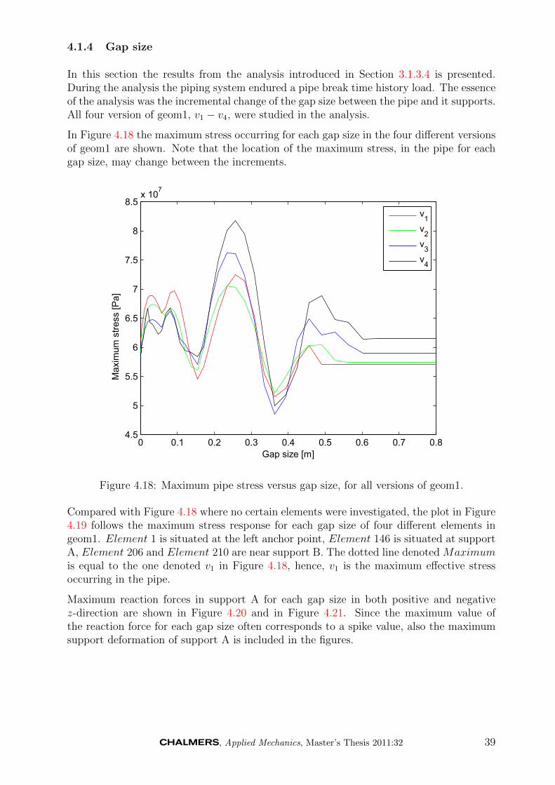
In this section the results from the analysis introduced in Section 3.1.3.4 is presented.During the analysis the piping system endured a pipe break time history load. The essenceof the analysis was the incremental change of the gap size between the pipe and it supports.All four version of geom1, v1 − v4, were studied in the analysis.
In Figure 4.18 the maximum stress occurring for each gap size in the four different versionsof geom1 are shown. Note that the location of the maximum stress, in the pipe for eachgap size, may change between the increments.
0 0.1 0.2 0.3 0.4 0.5 0.6 0.7 0.84.5
5
5.5
6
6.5
7
7.5
8
8.5x 10⁷
Gap size [m]
Max
imum
stre
ss [P
a]
v1v2v3v4
Figure 4.18: Maximum pipe stress versus gap size, for all versions of geom1.
Compared with Figure 4.18 where no certain elements were investigated, the plot in Figure4.19 follows the maximum stress response for each gap size of four different elements ingeom1. Element 1 is situated at the left anchor point, Element 146 is situated at supportA, Element 206 and Element 210 are near support B. The dotted line denoted Maximumis equal to the one denoted v1 in Figure 4.18, hence, v1 is the maximum effective stressoccurring in the pipe.
Maximum reaction forces in support A for each gap size in both positive and negativez-direction are shown in Figure 4.20 and in Figure 4.21. Since the maximum value ofthe reaction force for each gap size often corresponds to a spike value, also the maximumsupport deformation of support A is included in the figures.
, Applied Mechanics, Master’s Thesis 2011:32 39

0 0.1 0.2 0.3 0.4 0.5 0.60
1
2
3
4
5
6
7
8
9x 10⁷
Gap size [m]
Max
imum
stre
ss [P
a]
Element 1Element 146Element 206Element 210Maximum
Figure 4.19: Maximum pipe stress for four elements versus gap size together with themaximum stress for all elements, for version v1 of geom1.
0 0.1 0.2 0.3 0.4 0.5 0.60
1.1146
2.2292
3.3438
4.4584
5.5731x 10
6
Gap size [m]
Rea
ctio
n fo
rce
[N]
0 0.1 0.2 0.3 0.4 0.5 0.60
0.5413
1.0827
1.624
2.1653
2.7066x 10
-3D
efor
mat
ion
[m]
Max reaction forceSupport deformation
Figure 4.20: Maximum reaction force, and maximum deformation of support A in negativez-direction.
40 , Applied Mechanics, Master’s Thesis 2011:32

0 0.05 0.1 0.15 0.2 0.25 0.3 0.35 0.40
0.7879
1.5757
2.3636
3.1515
3.9393x 10
6
Gap size [m]
Rea
ctio
n fo
rce
[N]
0 0.05 0.1 0.15 0.2 0.25 0.3 0.35 0.40
0.3737
0.7473
1.121
1.4947
1.8683x 10
-3
Def
orm
atio
n [m
]
Max reaction forceSupport deformation
Figure 4.21: Maximum reaction force, and maximum deformation of support A in positivez-direction.
In Figure 4.22 the local maximum support deformation and maximum stress are marked,hence those points correspond to gap sizes where the supports and the pipe are exposedto high loads.
The time history results associated to those gap sizes for support A and B in geom1 v1are presented in the following figures: 4.23, 4.24. Both reaction force and stress are shownin the figures. The gap sizes corresponding to the highlighted points in Figure 4.22 arecompared to results with no gap in Figure 4.25 and 4.27. Standard support stiffness areused in both cases.
0 0.1 0.2 0.3 0.4 0.5 0.6 0.7 0.8 0.90
0.2
0.4
0.6
0.8
1
1.2
1.4
1.6
1.8x 10
-3
Gap size [m]
Max
sup
port
def
orm
atio
n [m
]
Support A in positive z-dirSupport A in negative z-dirSelected cases
0 0.1 0.2 0.3 0.4 0.5 0.6 0.7 0.84.5
5
5.5
6
6.5
7
7.5
8
8.5x 10⁷
Gap size [m]
Max
imum
stre
ss [P
a]
v1
Figure 4.22: Max support deformation and max stress versus gap size in geom1 v1, inves-tigated cases.
, Applied Mechanics, Master’s Thesis 2011:32 41

0 0.2 0.4 0.6 0.8 1 1.2 1.4 1.6 1.8 2-7.5838
-1.5168
4.5503
10.6173
16.6843
22.7513x 10⁵
Time [s]
Rea
ctio
n fo
rce
[N]
Gap size = 0 [mm]
0 0.2 0.4 0.6 0.8 1 1.2 1.4 1.6 1.8 2-1.4916
-0.2983
0.895
2.0883
3.2816
4.4749x 10⁷
Stre
ss [P
a]
Reaction force, positive z-dirReaction force, negative z-dirStress intesity
0 0.2 0.4 0.6 0.8 1 1.2 1.4 1.6 1.8 2-2.4021
-0.4804
1.4413
3.363
5.2847
7.2064x 10⁶
Time [s]
Rea
ctio
n fo
rce
[N]
Gap size = 4.86 [mm]
0 0.2 0.4 0.6 0.8 1 1.2 1.4 1.6 1.8 2-1.4262
-0.2852
0.8557
1.9967
3.1377
4.2787x 10⁷
Stre
ss [P
a]
Reaction force, positive z-dirReaction force, negative z-dirStress intesity
0 0.2 0.4 0.6 0.8 1 1.2 1.4 1.6 1.8 2-3.9393
-0.7879
2.3636
5.515
8.6665
11.818x 10⁶
Time [s]
Rea
ctio
n fo
rce
[N]
Gap size = 19.94 [mm]
0 0.2 0.4 0.6 0.8 1 1.2 1.4 1.6 1.8 2-1.5084
-0.3017
0.905
2.1117
3.3184
4.5251x 10⁷
Stre
ss [P
a]Reaction force, positive z-dirReaction force, negative z-dirStress intesity
0 0.2 0.4 0.6 0.8 1 1.2 1.4 1.6 1.8 2-8.8206
-1.7641
5.2923
12.3488
19.4053
26.4617x 10⁵
Time [s]
Rea
ctio
n fo
rce
[N]
Gap size = 79.79 [mm]
0 0.2 0.4 0.6 0.8 1 1.2 1.4 1.6 1.8 2-1.6474
-0.3295
0.9884
2.3063
3.6242
4.9421x 10⁷
Stre
ss [P
a]
Reaction force, positive z-dirReaction force, negative z-dirStress intesity
0 0.2 0.4 0.6 0.8 1 1.2 1.4 1.6 1.8 2-7.0791
-1.4158
4.2475
9.9107
15.574
21.2373x 10⁵
Time [s]
Rea
ctio
n fo
rce
[N]
Gap size = 275.1 [mm]
0 0.2 0.4 0.6 0.8 1 1.2 1.4 1.6 1.8 2-1.8528
-0.3706
1.1117
2.5939
4.0761
5.5583x 10⁷
Stre
ss [P
a]
Reaction force, positive z-dirReaction force, negative z-dirStress intesity
0 0.2 0.4 0.6 0.8 1 1.2 1.4 1.6 1.8 2-5.2478
-1.0496
3.1487
7.3469
11.5451
15.7434x 10⁵
Time [s]
Rea
ctio
n fo
rce
[N]
Gap size = 456.7 [mm]
0 0.2 0.4 0.6 0.8 1 1.2 1.4 1.6 1.8 2-1.6371
-0.3274
0.9823
2.292
3.6017
4.9114x 10⁷
Stre
ss [P
a]Reaction force, positive z-dirReaction force, negative z-dirStress intesity
Figure 4.23: Time history results, stress and reaction force at support A.
42 , Applied Mechanics, Master’s Thesis 2011:32

0 0.2 0.4 0.6 0.8 1 1.2 1.4 1.6 1.8 2-1.1067
-0.2213
0.664
1.5494
2.4348
3.3202x 10⁶
Time [s]
Rea
ctio
n fo
rce
[N]
Gap size = 0 [mm]
0 0.2 0.4 0.6 0.8 1 1.2 1.4 1.6 1.8 2-1.7315
-0.3463
1.0389
2.4241
3.8093
5.1945x 10⁷
Stre
ss [P
a]
Reaction force, positive x-dirReaction force, negative x-dirStress intesity
0 0.2 0.4 0.6 0.8 1 1.2 1.4 1.6 1.8 2-2.4021
-0.4804
1.4413
3.363
5.2847
7.2064x 10⁶
Time [s]
Rea
ctio
n fo
rce
[N]
Gap size = 4.86 [mm]
0 0.2 0.4 0.6 0.8 1 1.2 1.4 1.6 1.8 2-1.4262
-0.2852
0.8557
1.9967
3.1377
4.2787x 10⁷
Stre
ss [P
a]
Reaction force, positive x-dirReaction force, negative x-dirStress intesity
0 0.2 0.4 0.6 0.8 1 1.2 1.4 1.6 1.8 2-3.2184
-0.6437
1.931
4.5058
7.0805
9.6552x 10⁶
Time [s]
Rea
ctio
n fo
rce
[N]
Gap size = 19.94 [mm]
0 0.2 0.4 0.6 0.8 1 1.2 1.4 1.6 1.8 2-1.8595
-0.3719
1.1157
2.6033
4.0909
5.5784x 10⁷
Stre
ss [P
a]Reaction force, positive x-dirReaction force, negative x-dirStress intesity
0 0.2 0.4 0.6 0.8 1 1.2 1.4 1.6 1.8 2-1.033
-0.2066
0.6198
1.4463
2.2727
3.0991x 10⁶
Time [s]
Rea
ctio
n fo
rce
[N]
Gap size = 79.79 [mm]
0 0.2 0.4 0.6 0.8 1 1.2 1.4 1.6 1.8 2-1.9073
-0.3815
1.1444
2.6702
4.1961
5.7219x 10⁷
Stre
ss [P
a]
Reaction force, positive x-dirReaction force, negative x-dirStress intesity
0 0.2 0.4 0.6 0.8 1 1.2 1.4 1.6 1.8 2-8.1177
-1.6235
4.8706
11.3648
17.8589
24.353x 10⁵
Time [s]
Rea
ctio
n fo
rce
[N]
Gap size = 275.1 [mm]
0 0.2 0.4 0.6 0.8 1 1.2 1.4 1.6 1.8 2-5.0393
-1.0079
3.0236
7.055
11.0865
15.118x 10⁶
Stre
ss [P
a]
Reaction force, positive x-dirReaction force, negative x-dirStress intesity
0 0.2 0.4 0.6 0.8 1 1.2 1.4 1.6 1.8 2-1
-0.6
-0.2
0.2
0.6
1
Time [s]
Rea
ctio
n fo
rce
[N]
Gap size = 456.7 [mm]
0 0.2 0.4 0.6 0.8 1 1.2 1.4 1.6 1.8 2-4.8673
-0.9735
2.9204
6.8142
10.708
14.6018x 10⁶
Stre
ss [P
a]Reaction force, positive x-dirReaction force, negative x-dirStress intesity
Figure 4.24: Time history results, stress and reaction force at support B.
, Applied Mechanics, Master’s Thesis 2011:32 43

0 0.2 0.4 0.6 0.8 1-2.5
-2
-1.5
-1
-0.5
0
0.5
1
1.5
2x 10⁶
Time [s]
Rea
ctio
n fo
rce
[N]
No gap4.8mm gap
0 0.2 0.4 0.6 0.8 10
0.5
1
1.5
2
2.5
3
3.5
4
4.5x 10⁷
Time [s]
Stre
ss [P
a]
No gap4.8mm gap
Figure 4.25: Time history of effective Tresca stress and force in support A, gap = 4.86mm.
0 0.2 0.4 0.6 0.8 1-4
-3
-2
-1
0
1
2
3x 10⁶
Time [s]
Rea
ctio
n fo
rce
[N]
No gap19.9mm gap
0 0.2 0.4 0.6 0.8 10
0.5
1
1.5
2
2.5
3
3.5
4
4.5x 10⁷
Time [s]
Stre
ss [P
a]
No gap19.9mm gap
Figure 4.26: Time history of effective Tresca stress and force in support A, gap = 19.91mm.
44 , Applied Mechanics, Master’s Thesis 2011:32

0 0.2 0.4 0.6 0.8 1-8
-6
-4
-2
0
2
4
6
8x 10⁵
Time [s]
Rea
ctio
n fo
rce
[N]
No gap257.1mm gap
0 0.2 0.4 0.6 0.8 10
1
2
3
4
5
6x 10⁷
Time [s]
Stre
ss [P
a]
No gap257.1mm gap
Figure 4.27: Time history of effective Tresca stress and force in support A, gap = 257.1mm.
As previously mentioned, the time history of the reaction force often shows spike charac-teristics, for example displayed in Figure 4.26. The reaction force closely related supportdeformation is compared to the reaction force in Figure 4.28 and 4.29.
0 0.2 0.4 0.6 0.8 1 1.2 1.4 1.6 1.8 2-6.5232
0
6.5232
13.0464
19.5696
26.0928x 10
5
Time [s]
Rea
ctio
n fo
rce
[N]
0 0.2 0.4 0.6 0.8 1 1.2 1.4 1.6 1.8 2-0.8193
0
0.8193
1.6386
2.4579
3.2772x 10
-3
Sup
port
def
orm
atio
n [m
]
Reaction force, positive z-dirSupport deformation
Figure 4.28: Time history of reaction force in negative z-direction and support deformationin support A, gap = 19.91 mm.
, Applied Mechanics, Master’s Thesis 2011:32 45

0 0.2 0.4 0.6 0.8 1 1.2 1.4 1.6 1.8 2-0.9848
0
0.9848
1.9697
2.9545
3.9393x 10
6
Time [s]
Rea
ctio
n fo
rce
[N]
0 0.2 0.4 0.6 0.8 1 1.2 1.4 1.6 1.8 2-0.8716
0
0.8716
1.7431
2.6147
3.4863x 10
-3
Sup
port
def
orm
atio
n [m
]
Reaction force, positive z-dirSupport deformation
Figure 4.29: Time history of reaction force in positive z-direction and support deformationin support A, gap = 19.91 mm.
4.1.5 Stiffness approximations
It was investigated if one could approximate the behavior of a gap support by varying thestiffness of support without a gap. In Figure 4.30 one can see a plot of the reaction force atsupport A and the stress of an adjacent element. Two systems with standard stiffness wereanalyzed, one with and one without gaps. Also, a gap system with 21.9kN/mm stiffnesswas analyzed. A problem that arose was how to measure the correlation between a systemwith a gap and one without. As can be seen in Figure 4.30, the appearance of the gap andno-gap curves are quite different. If one was to smoothen the curves from the gap analysis,and thereby remove the spikes, the correlation between the two 700 kN/mm curves wouldbe good.
0 0.2 0.4 0.6 0.8 1-2.5
-2
-1.5
-1
-0.5
0
0.5
1
1.5
2
2.5
3x 10⁶
Time [s]
Rea
ctio
n fo
rce
[N]
4.8mm gap, 700kN/mm stiffnessNo gap, 21.9kN/mm stiffnessNo gap, 700kN/mm stiffness
0 0.2 0.4 0.6 0.8 10
0.5
1
1.5
2
2.5
3
3.5
4
4.5
5
5.5x 10⁷
Time [s]
Stre
ss [P
a]
4.8mm gap, 700kN/mm stiffnessNo gap, 21.9kN/mm stiffnessNo gap, 700kN/mm stiffness
Figure 4.30: Time history of reaction force and stress for different stiffness-gap configura-tions.
46 , Applied Mechanics, Master’s Thesis 2011:32
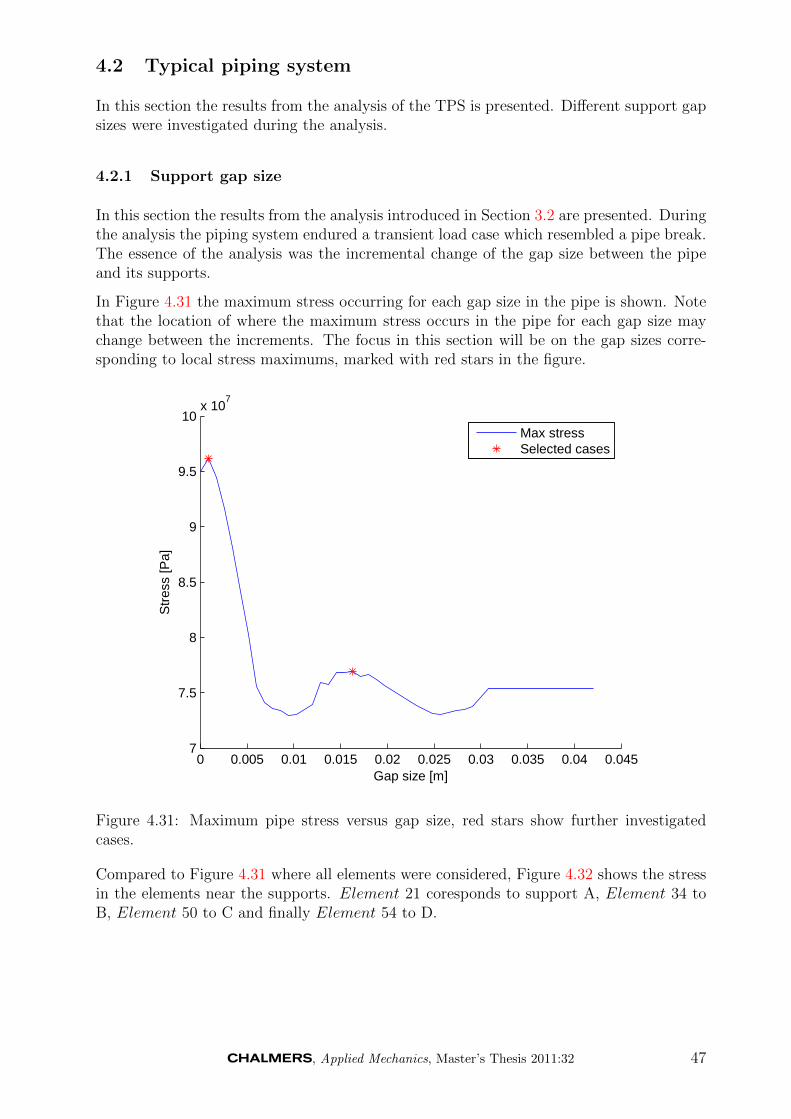
4.2 Typical piping system
In this section the results from the analysis of the TPS is presented. Different support gapsizes were investigated during the analysis.
4.2.1 Support gap size
In this section the results from the analysis introduced in Section 3.2 are presented. Duringthe analysis the piping system endured a transient load case which resembled a pipe break.The essence of the analysis was the incremental change of the gap size between the pipeand its supports.
In Figure 4.31 the maximum stress occurring for each gap size in the pipe is shown. Notethat the location of where the maximum stress occurs in the pipe for each gap size maychange between the increments. The focus in this section will be on the gap sizes corre-sponding to local stress maximums, marked with red stars in the figure.
0 0.005 0.01 0.015 0.02 0.025 0.03 0.035 0.04 0.0457
7.5
8
8.5
9
9.5
10x 10
7
Gap size [m]
Str
ess
[Pa]
Max stressSelected cases
Figure 4.31: Maximum pipe stress versus gap size, red stars show further investigatedcases.
Compared to Figure 4.31 where all elements were considered, Figure 4.32 shows the stressin the elements near the supports. Element 21 coresponds to support A, Element 34 toB, Element 50 to C and finally Element 54 to D.
, Applied Mechanics, Master’s Thesis 2011:32 47

0 0.005 0.01 0.015 0.02 0.025 0.03 0.035 0.04 0.0450.5
1
1.5
2
2.5
3
3.5
4x 10
7
Gap size [m]
Str
ess
[Pa]
Element 21Element 34Element 50Element 56
Figure 4.32: Maximum pipe stress versus gap size in elements near the supports.
The time history results associated to those gap sizes for support A - D are presented inthe following figures: 4.33 - 4.36. Both reaction force and stress are shown in the figures.
0 1 2 3 4 5 6 7 8 9 10-1.2149
-0.729
-0.243
0.243
0.729
1.2149x 10
5
Time [s]
Rea
ctio
n fo
rce
[N]
Support 1 - Gap size = 8.5714e-004 [m]
0 1 2 3 4 5 6 7 8 9 10-2.3373
-1.4024
-0.4675
0.4675
1.4024
2.3373x 10
7
Str
ess
inte
nsity
[Pa]
Reaction force, positive z-dirReaction force, negative z-dirStress intesity
0 1 2 3 4 5 6 7 8 9 10-5138.0864
-3082.8518
-1027.6173
1027.6173
3082.8518
5138.0864
Time [s]
Rea
ctio
n fo
rce
[N]
Support 1 - Gap size = 0.0163 [m]
0 1 2 3 4 5 6 7 8 9 10-2.6409
-1.5845
-0.5282
0.5282
1.5845
2.6409x 10
7
Str
ess
inte
nsity
[Pa]
Reaction force, positive z-dirReaction force, negative z-dirStress intesity
Figure 4.33: Time history results for stress and reaction force at support A.
0 1 2 3 4 5 6 7 8 9 10-1.2832
-0.7699
-0.2566
0.2566
0.7699
1.2832x 10
5
Time [s]
Rea
ctio
n fo
rce
[N]
Support 1 - Gap size = 8.5714e-004 [m]
0 1 2 3 4 5 6 7 8 9 10-3.2361
-1.9416
-0.6472
0.6472
1.9416
3.2361x 10
5
Time [s]
Rea
ctio
n fo
rce
[N]
Support 1 - Gap size = 0.0163 [m]
0 1 2 3 4 5 6 7 8 9 10-2.7242
-1.6345
-0.5448
0.5448
1.6345
2.7242x 10
7
Str
ess
inte
nsity
[Pa]
Reaction force, positive z-dirReaction force, negative z-dirStress intesity
0 1 2 3 4 5 6 7 8 9 10-3.1407
-1.8844
-0.6281
0.6281
1.8844
3.1407x 10
7
Str
ess
inte
nsity
[Pa]
Reaction force, positive z-dirReaction force, negative z-dirStress intesity
Figure 4.34: Time history results for stress and reaction force at support B.
48 , Applied Mechanics, Master’s Thesis 2011:32

0 1 2 3 4 5 6 7 8 9 10-2.8253
-1.6952
-0.5651
0.5651
1.6952
2.8253x 10
5
Time [s]
Rea
ctio
n fo
rce
[N]
Support 1 - Gap size = 8.5714e-004 [m]
0 1 2 3 4 5 6 7 8 9 10-3.4009
-2.0405
-0.6802
0.6802
2.0405
3.4009x 10
7
Str
ess
inte
nsity
[Pa]
Reaction force, positive z-dirReaction force, negative z-dirStress intesity
0 1 2 3 4 5 6 7 8 9 10-3.9324
-2.3595
-0.7865
0.7865
2.3595
3.9324x 10
5
Time [s]
Rea
ctio
n fo
rce
[N]
Support 1 - Gap size = 0.0163 [m]
0 1 2 3 4 5 6 7 8 9 10-1.7696
-1.0618
-0.3539
0.3539
1.0618
1.7696x 10
7
Str
ess
inte
nsity
[Pa]
Reaction force, positive z-dirReaction force, negative z-dirStress intesity
Figure 4.35: Time history results for stress and reaction force at support C.
0 1 2 3 4 5 6 7 8 9 10-3.0572
-1.8343
-0.6114
0.6114
1.8343
3.0572x 10
5
Time [s]
Rea
ctio
n fo
rce
[N]
Support 1 - Gap size = 8.5714e-004 [m]
0 1 2 3 4 5 6 7 8 9 10-3.2691
-1.9614
-0.6538
0.6538
1.9614
3.2691x 10
7
Str
ess
inte
nsity
[Pa]
Reaction force, positive z-dirReaction force, negative z-dirStress intesity
0 5 10 15-1
-0.6
-0.2
0.2
0.6
1
Time [s]
Rea
ctio
n fo
rce
[N]
Support 1 - Gap size = 0.0163 [m]
0 1 2 3 4 5 6 7 8 9 10-1.3041
-0.7825
-0.2608
0.2608
0.7825
1.3041x 10
7
Str
ess
inte
nsity
[Pa]
Reaction force, positive z-dirReaction force, negative z-dirStress intesity
Figure 4.36: Time history results for stress and reaction force at support D.
In Figure 4.37 - 4.40 the results for gap sizes corresponding to the highlighted cases inFigure 4.31 are compared to the results for no gap. Standard support stiffness are used inall cases.
0 0.5 1 1.5 2 2.5 3 3.5 4-1.5
-1
-0.5
0
0.5
1
1.5
2
2.5
3
3.5x 10
5
Time [s]
Rea
ctio
n fo
rce
[N]
No gap5.1 mm gap
0 0.5 1 1.5 2 2.5 3 3.5 40
0.5
1
1.5
2
2.5x 10
7
Time [s]
Str
ess
[Pa]
No gap5.1 mm gap
0 0.5 1 1.5 2 2.5 3 3.5 4-14
-12
-10
-8
-6
-4
-2
0
2
4x 10
4
Time [s]
Rea
ctio
n fo
rce
[N]
No gap16.3 mm gap
0 0.5 1 1.5 2 2.5 3 3.5 40
0.5
1
1.5
2
2.5x 10
7
Time [s]
Str
ess
[Pa]
No gap16.3 mm gap
Figure 4.37: Time history results, stress and reaction force at support A, .
, Applied Mechanics, Master’s Thesis 2011:32 49

0 0.5 1 1.5 2 2.5 3 3.5 4-2
-1.5
-1
-0.5
0
0.5
1
1.5
2
2.5x 10
5
Time [s]
Rea
ctio
n fo
rce
[N]
No gap5.1 mm gap
0 0.5 1 1.5 2 2.5 3 3.5 40
0.5
1
1.5
2
2.5
3x 10
7
Time [s]
Str
ess
[Pa]
No gap5.1 mm gap
0 0.5 1 1.5 2 2.5 3 3.5 4-6
-5
-4
-3
-2
-1
0
1
2
3x 10
5
Time [s]
Rea
ctio
n fo
rce
[N]
No gap16.3 mm gap
0 0.5 1 1.5 2 2.5 3 3.5 40
0.5
1
1.5
2
2.5
3x 10
7
Time [s]S
tres
s [P
a]
No gap16.3 mm gap
Figure 4.38: Time history results for stress and reaction force at support B.
0 0.5 1 1.5 2 2.5 3 3.5 4-1.5
-1
-0.5
0
0.5
1
1.5
2
2.5
3
3.5x 10
5
Time [s]
Rea
ctio
n fo
rce
[N]
No gap5.1 mm gap
0 0.5 1 1.5 2 2.5 3 3.5 40
0.5
1
1.5
2
2.5x 10
7
Time [s]
Str
ess
[Pa]
No gap5.1 mm gap
0 0.5 1 1.5 2 2.5 3 3.5 4-14
-12
-10
-8
-6
-4
-2
0
2
4x 10
4
Time [s]
Rea
ctio
n fo
rce
[N]
No gap16.3 mm gap
0 0.5 1 1.5 2 2.5 3 3.5 40
0.5
1
1.5
2
2.5x 10
7
Time [s]
Str
ess
[Pa]
No gap16.3 mm gap
Figure 4.39: Time history results for stress and reaction force at support C.
50 , Applied Mechanics, Master’s Thesis 2011:32

0 0.5 1 1.5 2 2.5 3 3.5 4-1.5
-1
-0.5
0
0.5
1
1.5
2
2.5
3
3.5x 10
5
Time [s]
Rea
ctio
n fo
rce
[N]
No gap5.1 mm gap
0 0.5 1 1.5 2 2.5 3 3.5 40
0.5
1
1.5
2
2.5x 10
7
Time [s]
Str
ess
[Pa]
No gap5.1 mm gap
0 0.5 1 1.5 2 2.5 3 3.5 4-14
-12
-10
-8
-6
-4
-2
0
2
4x 10
4
Time [s]
Rea
ctio
n fo
rce
[N]
No gap16.3 mm gap
0 0.5 1 1.5 2 2.5 3 3.5 40
0.5
1
1.5
2
2.5x 10
7
Time [s]
Str
ess
[Pa]
No gap16.3 mm gap
Figure 4.40: Time history results for stress and reaction force at support D.
4.3 Validation
After analyzing both the simplified piping system and the typical piping system in ANSYSand Pipestress with similar conditions, it was concluded that the two analyzes correlated.All validation parameters were compared and the differences were low. The only parameterthat showed a noticeable difference was the element stresses from a pipe break analysis.These differences were due to different stress intensification factors in the bend and theywere accounted for when the gap analysis results were post processed.
, Applied Mechanics, Master’s Thesis 2011:32 51

52 , Applied Mechanics, Master’s Thesis 2011:32

5 Conclusions and Discussion
In the time step analysis it appeared that it was very difficult to resolve the short durationreaction force that frequently appeared at first contact between the pipe and its supports.The amplitude of the reaction force spikes did not converge even if the time step wasdecreased until the practical limit for computational time. But on the other hand, if oneinstead considers the convergence of maximum stress in the pipe, it is more satisfying.The stress converges rapidly even at quite large time steps. If the characteristics of atime history element stress result is compared to a time history reaction force result, thesimilarities are striking, except on one point, the reaction force spikes.
Analysis was performed both with and without friction. Due to lengthy analyses, thenumber of gap sizes were limited. The selected set of gap sizes were chosen on the base ofmaximum support deformation. Despite the close connection between force and deflectionit turned out that the support deformation did not show the same characteristic spikesas the reaction force, hence maximum support deformation was used when the gap sizeswere chosen. The results, when friction in the contact between the pipe and its supportwere accounted for, indicate that the condition works satisfactory. For example, whencomparing the displacement curves with and without friction, the energy loss from thepipe in the case of friction is noticeable. The general behavior of the pipe stresses is thatthey are lower when friction is accounted for due to energy loss. This indicates that it isa reasonable assumption to neglect friction in this kind of analysis.
The majority of all analyses performed in this thesis have been conducted using standardsupport stiffnesses, but due to the reaction force spikes and the question of how well it ispossible to approximate a support gap with a spring, the influence of support stiffness hasbeen investigated. First lets consider the relationship between support stiffness, when agap exists, and reaction force spikes. When the support stiffness was lowered to one thirdof the standard stiffness, the spike characteristics disappeared due to lower accelerationin the impact. The other part of the reaction force, not the one associated with highacceleration immediately after impact but the long lasting one, is much less affected by thechange in support stiffness. The computational time was decreased when weaker springstiffnesses were used. This was in line with results reported in [14].
The essence of this thesis is the investigation regarding the influence of support gap sizein a elastic piping systems. For example the question being raised in the introduction,weather it is conservative to neglect support gaps if the size is less then five millimeter?The analyses done on the geometry that was constructed to resemble a typical steamsystem indicate that it is not conservative to neglect gaps, with respect to reaction force,if the spikes were taken into account. Throughout this thesis, caution has been used whenexamining the force spike results. If the reaction force spikes are neglected, the resultsindicate that it is realistic assumption to neglect gap up to 5mm, both considering pipestresses and support reaction forces.
How good is the correlation with larger gaps typically found in pipe break anchors forgaps larger than five millimeter? The simplified model shows results equally as for smallgaps; if the spikes due to impact are neglected, one can neglect a support gap. In termsof stresses in the pipe system, it is even a slightly conservative approximation to neglectgaps. But if the spikes are considered, the maximum stress levels with a gap size equal to20-40 millimeter increases with 20-30% in the studied simplified system and the reactionforces increases with up to 300%.
, Applied Mechanics, Master’s Thesis 2011:32 53

The simplified geometry analyzed indicates that both for small gaps, up to 5 mm, andgaps larger than 5 mm the approximation to neglect gaps gives best result if the supportstiffness is equal in the approximative analysis as in the gap analysis, if the impact spikesare neglected. If the spikes are considered, it is possible that a lower spring stiffness ispreferred due to its effect on the spike characteristic as previously mentioned.
During this thesis, many different contact elements were evaluated. In the final analysis,Conta178 was used to model the gap because of good setup options, possibility to modelcontact friction and possibilities to use different contact methods. However, the moststraight forward contact element to work with was the Combin40 element. The downsideto Combin40 is the lack of possible settings, for example the inability to choose contactmethod. Although, for faster analyses, it is a good alternative to Conta178.
54 , Applied Mechanics, Master’s Thesis 2011:32

6 Recommendations
For further work in this area we have the following recommendations:
• Use a elasto-plastic material model, in the contact surfaces and examine the plasticzone.
• Perform an explicit analysis to better resolve the fast contact forces that appear ingap support models. This could be done using, for example, LS-DYNA Explicit.
• Make a more detailed FEM model of the supports and pipe. Use smaller solid orshell elements instead of the pipe, beam elements, that were used in this thesis. Thiswould lead to better knowledge about the stresses in the supports.
• Try to use a simpler load, for example, sinus shaped loads with different frequencies.This would give a better picture of how the results depend on the load case and itsfrequency range. By raising the the frequency of a half period sinus load, the effectof force spikes could also be investigated.
• The pipe break load in the simplified pinging system was calculated with steam asthe fluid. Try a similar load with water as the fluid.
• Analyze a larger amount of pipe systems with different loads to get results that arereliable and to be able to make better conclusions.
• Try other kinds of supports with other kinds of stiffness nonlinearities. This thesisonly considers rigid restrains. For example, a spring support that reaches maximumcompression, with resulting stiffness increase, could be interesting.
• Investigate if there is a more realistic way to model the damping. A Rayleigh damp-ing, approximated to reassemble a constant damping of 5% may not be optimal fromthis point of view.
, Applied Mechanics, Master’s Thesis 2011:32 55

56 , Applied Mechanics, Master’s Thesis 2011:32

References
[1] Ansys. http://www.ansys.com.
[2] Ansys release 11.0 documentation for ansys. http://www.ansys.com.
[3] Asme. http://www.asme.net.
[4] Pipestress. http://www.dst.ch/.
[5] Asme section iii, rules of nuclear power plant components, division 1 - subsection nc,article nf-1000, nc-1132. http://www.asme.net, 1995.
[6] Asme section ii,rules of nuclear power plant components, part d. http://www.asme.
net, 2003.
[7] Klaus-Jurgen Bathe. Finite Element Procedures in Engineering Analysis. Prentice-Hall,Englewood Cliffs, New Jersey, 1982.
[8] Javier Bonet and Richard D. Wood. Nonlinear Continuum Mechanics for FiniteElement Analysis 2nd edition. Cambridge University Press, 2008.
[9] David Hutton. Fundamentals of Finite Element Analysis. The McGraw Hill Compa-nies, Washington, 2004.
[10] Benjamin R. STRONG Jr. and Ronald J. BASCHIERE. Pipe rupture and steam/waterhammer design loads for dynamic analysis of piping systems. Advanced AnalysisDivision, EDS Nuclear Inc., San Francisco, 1977.
[11] Igli Micheli and Piero Zanaboni. An analytical validation of simplified methods forthe assessment of pipe whip characteristics, 2003.
[12] Niels Ottosen and Hans Petersson. Introduction to the Finite Element Method. Pren-tice Hall Europe, 1992.
[13] Paul R. Smith and Thomas J. Van Laan. Piping and pipe support systems: designand engineering. McGraw Hill Book Co.,New York, NY, 1987.
[14] Hsiang-Chuan Tsai and Ming-Kuen Wu. Methods to compute dynamic response ofcantilever with a stop to limit motion. Department of Construction Engineering, Na-tional Taiwan Institute of Technology, Tapei, 1994.
[15] Jr. William Weaver and James M. Gere. Matrix Analysis Of Framed Structures, 3rdEdition. Springer-Verlag New York, LLC, 1966.
[16] Peter Wriggers. Computational contact mechanics, second edition. Springer, BerlinHeidelberg New York, 2006.
[17] Peter Wriggers. Nonlinear Finite Element Methods. Springer, Berlin Heidelberg, 2008.
, Applied Mechanics, Master’s Thesis 2011:32 57

58 , Applied Mechanics, Master’s Thesis 2011:32

A Simplified piping system, time history force
In this Appendix the resulting time history force components from the pipe break ingeom1 v1 − geom1 v4 are shown in the figures below.
0 0.1 0.2 0.3 0.4 0.5-6
-5
-4
-3
-2
-1
0
1x 10
5
time [s]
F1 [N
]
0 0.1 0.2 0.3 0.4 0.5-4
-3.5
-3
-2.5
-2
-1.5
-1
-0.5
0
0.5x 10
5
time [s]F
2 [N]
0 0.1 0.2 0.3 0.4 0.5-6
-5
-4
-3
-2
-1
0
1x 10
5
time [s]
F3 [N
]
0 0.1 0.2 0.3 0.4 0.5-7
-6
-5
-4
-3
-2
-1
0
1x 10
5
time [s]
F4 [N
]
0 0.1 0.2 0.3 0.4 0.5-10
-8
-6
-4
-2
0
2x 10
5
time [s]
F5 [N
]
Figure A.1: Time history force components of geom1 v1.
, Applied Mechanics, Master’s Thesis 2011:32 59

0 0.1 0.2 0.3 0.4 0.5-6
-5
-4
-3
-2
-1
0
1x 10
5
time [s]
F1 [N
]
0 0.1 0.2 0.3 0.4 0.5-4
-3.5
-3
-2.5
-2
-1.5
-1
-0.5
0
0.5x 10
5
time [s]
F2 [N
]
0 0.1 0.2 0.3 0.4 0.5-6
-5
-4
-3
-2
-1
0
1x 10
5
time [s]
F3 [N
]
0 0.1 0.2 0.3 0.4 0.5-7
-6
-5
-4
-3
-2
-1
0
1x 10
5
time [s]
F4 [N
]
0 0.1 0.2 0.3 0.4 0.5-10
-8
-6
-4
-2
0
2x 10
5
time [s]
F5 [N
]
Figure A.2: Time history force components of geom1 v2.
60 , Applied Mechanics, Master’s Thesis 2011:32

0 0.1 0.2 0.3 0.4 0.5-6
-5
-4
-3
-2
-1
0
1x 10
5
time [s]
F1 [N
]
0 0.1 0.2 0.3 0.4 0.5-5
-4
-3
-2
-1
0
1x 10
5
time [s]
F2 [N
]
0 0.1 0.2 0.3 0.4 0.5-6
-5
-4
-3
-2
-1
0
1x 10
5
time [s]
F3 [N
]
0 0.1 0.2 0.3 0.4 0.5-7
-6
-5
-4
-3
-2
-1
0
1x 10
5
time [s]
F4 [N
]
0 0.1 0.2 0.3 0.4 0.5-10
-8
-6
-4
-2
0
2x 10
5
time [s]
F5 [N
]
Figure A.3: Time history force components of geom1 v3.
, Applied Mechanics, Master’s Thesis 2011:32 61
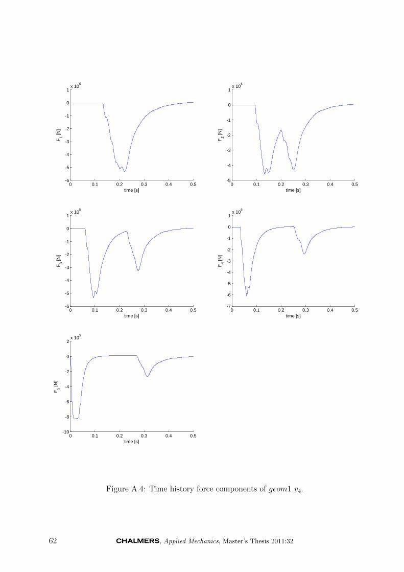
0 0.1 0.2 0.3 0.4 0.5-6
-5
-4
-3
-2
-1
0
1x 10
5
time [s]
F1 [N
]
0 0.1 0.2 0.3 0.4 0.5-5
-4
-3
-2
-1
0
1x 10
5
time [s]
F2 [N
]
0 0.1 0.2 0.3 0.4 0.5-6
-5
-4
-3
-2
-1
0
1x 10
5
time [s]
F3 [N
]
0 0.1 0.2 0.3 0.4 0.5-7
-6
-5
-4
-3
-2
-1
0
1x 10
5
time [s]
F4 [N
]
0 0.1 0.2 0.3 0.4 0.5-10
-8
-6
-4
-2
0
2x 10
5
time [s]
F5 [N
]
Figure A.4: Time history force components of geom1 v4.
62 , Applied Mechanics, Master’s Thesis 2011:32

B Simplified piping system, time history force
This Appendix contains the resulting time history force components from the pipe breakin the typical piping system. The figures show the resulting absolute forces of the x,y andz components in nine points of the pipe.
0 1 2 3 4 5 60
1
2
3
4
5
6
7
8
9
10x 10
4
Time [s]
F1 [N
]
0 1 2 3 4 5 60
2
4
6
8
10
12x 10
4
Time [s]
F2 [N
]
0 1 2 3 4 5 60
2
4
6
8
10
12x 10
4
Time [s]
F3 [N
]
Figure B.1: Time history force components of the typical piping system, F1-F3
, Applied Mechanics, Master’s Thesis 2011:32 63

0 1 2 3 4 5 60
2
4
6
8
10
12
14x 10
4
Time [s]
F4 [N
]
0 1 2 3 4 5 60
2
4
6
8
10
12
14x 10
4
Time [s]
F5 [N
]
0 1 2 3 4 5 60
2
4
6
8
10
12
14x 10
4
Time [s]
F6 [N
]
Figure B.2: Time history force components of the typical piping system, F4-F6
64 , Applied Mechanics, Master’s Thesis 2011:32

0 1 2 3 4 5 60
2
4
6
8
10
12x 10
4
Time [s]
F7 [N
]
0 1 2 3 4 5 60
2
4
6
8
10
12
14
16
18x 10
4
Time [s]
F8 [N
]
0 1 2 3 4 5 60
1
2
3
4
5
6
7
8x 10
4
Time [s]
F9 [N
]
Figure B.3: Time history force components of the typical piping system, F7-F9
, Applied Mechanics, Master’s Thesis 2011:32 65

66 , Applied Mechanics, Master’s Thesis 2011:32

C Standard support stiffness
The table below includes generally accepted standard support stiffnesses from the Swedishnuclear power plant industry.
, Applied Mechanics, Master’s Thesis 2011:32 67