Inferring catchment precipitation by doing hydrology...

Inferring catchment precipitation by doing hydrology backward:A test in 24 small and mesoscale catchments in Luxembourg

R. Krier,1,2 P. Matgen,1 K. Goergen,1 L. Pfister,1 L. Hoffmann,1 J. W. Kirchner,3,4,5

S. Uhlenbrook,2,6 and H. H. G. Savenije2

Received 15 March 2011; revised 13 August 2012; accepted 2 September 2012; published 10 October 2012.

[1] The complexity of hydrological systems and the necessary simplification of modelsdescribing these systems remain major challenges in hydrological modeling. Kirchner’s(2009) approach of inferring rainfall and evaporation from discharge fluctuations by‘‘doing hydrology backward’’ is based on the assumption that catchment behavior canbe conceptualized with a single storage-discharge relationship. Here we test Kirchner’sapproach using a densely instrumented hydrologic measurement network spanning24 geologically diverse subbasins of the Alzette catchment in Luxembourg. We show thateffective rainfall rates inferred from discharge fluctuations generally correlate well withcatchment-averaged precipitation radar estimates in catchments ranging from less than10 to more than 1000 km2 in size. The correlation between predicted and observed effectiveprecipitation was 0.8 or better in 23 of our 24 catchments, and prediction skill did not varysystematically with catchment size or with the complexity of the underlying geology.Model performance improves systematically at higher soil moisture levels, indicating thatour study catchments behave more like simple dynamical systems with unambiguousstorage-discharge relationships during wet conditions. The overall mean correlationcoefficient for all subbasins for the entire data set increases from 0.80 to 0.95, and the meanbias for all basins decreases from –0.61 to –0.35 mm d�1. We propose an extension ofKirchner’s approach that uses in situ soil moisture measurements to distinguish wet and drycatchment conditions.

Citation: Krier, R., P. Matgen, K. Goergen, L. Pfister, L. Hoffmann, J. W. Kirchner, S. Uhlenbrook, and H. H. G. Savenije (2012),

Inferring catchment precipitation by doing hydrology backward: A test in 24 small and mesoscale catchments in Luxembourg, WaterResour. Res., 48, W10525, doi:10.1029/2011WR010657.

1. Introduction[2] Every hydrological modeler strives to overcome the

inherent complexity and heterogeneity of hydrologicalprocesses by making appropriate modeling simplificationsand generalizations. In one recent effort along these lines,Kirchner [2009] showed that if a catchment can bedescribed by a single storage element in which discharge is afunction of storage alone, this storage-discharge relation canbe estimated from streamflow fluctuations. Kirchner [2009]demonstrated that in such simple dynamical systems, it is

possible to ‘‘do hydrology backward,’’ that is, to infer rain-fall and evaporation time series from discharge fluctuationsalone. Although the effect of evaporation and plant transpi-ration on runoff recession has been studied previously indetail [e.g., Federer, 1973; Daniel, 1976; Brutsaert, 1982],the ‘‘hydrology backward’’ approach offers interesting newpossibilities for catchment hydrology and merits further test-ing in catchments characterized by different climates andlithologies. Teuling et al. [2010] have recently investigatedthe ‘‘hydrology backward’’ approach in the Swiss Rietholz-bach catchment, observing that the model performed betterunder wet conditions. Kirchner [2009] has also pointed outthat the approach should begin to break down in catchmentsthat are larger than individual storm systems, due to the factthat a model that represents a basin as a single nonlinearstorage will not easily encompass cases in which one part ofthe basin can be completely saturated after a storm whileanother part remains dry. However, given that the hydrologybackward approach has so far been applied in relativelysmall catchments like Plynlimon (�10 km2) in Wales[Kirchner, 2009] and Rietholzbach (�3 km2) in Switzerland[Teuling et al., 2010], it has been unclear whether theapproach can be used successfully in much larger basins.

[3] Here we investigate the advantages and limitations ofthe ‘‘hydrology backward’’ approach in a densely instru-mented network of geologically diverse catchments, inferring

1Public Research Center–Gabriel Lippmann, Belvaux, Luxembourg.2Water Resources Section, Faculty of Civil Engineering and Geoscien-

ces, Delft University of Technology, Delft, Netherlands.3Department of Earth and Planetary Science, University of California,

Berkeley, California, USA.4Swiss Federal Institute for Forest, Snow, and Landscape Research

WSL, Birmensdorf, Switzerland.5Department of Environmental System Sciences, ETH Zurich, Zurich,

Switzerland.6Department of Water Engineering, UNESCO-IHE, Delft, Netherlands.

Corresponding author: R. Krier, Public Research Center–Gabriel Lipp-mann, 41 Rue du Brill, LU-4422 Belvaux, Luxembourg. ([email protected])

©2012. American Geophysical Union. All Rights Reserved.0043-1397/12/2011WR010657

W10525 1 of 15

WATER RESOURCES RESEARCH, VOL. 48, W10525, doi:10.1029/2011WR010657, 2012

http://dx.doi.org/10.1029/2011WR010657

catchment average rainfall rates from streamflow fluctuationsand testing them against weather radar rainfall data that pro-vide more representative catchment average precipitationmeasurements than interpolated point measurements do.Although Kirchner [2009] already presented a virtual experi-ment that applied the approach to a hypothetical storm withdifferent antecedent moisture levels (i.e., storage levels) todemonstrate the concept that peak runoff can be estimatedfrom the sensitivity function, we go a step further by using insitu soil moisture measurements as a proxy for the catchmentstorage status, in order to investigate the impact that anteced-ent soil moisture conditions have on model performance.

[4] In summary this paper has two main objectives: (1)to understand the limitations and advantages of Kirchner’s[2009] approach with respect to different catchment charac-teristics (e.g., basin size, lithology) and soil wetness condi-tions and (2) to assess the potential of the approach fordiagnosing the functioning of hydrological systems and tocompare model behavior under various catchment conditions.

2. Methods2.1. Kirchner’s Methodology

[5] The methodology outlined by Kirchner [2009] com-bines the conservation of mass equation (1) and theassumption that the stream discharge Q depends solely onthe amount of water S stored in the catchment, quantifiedby a deterministic storage-discharge function (2):

dS

dt¼ P� E � Q (1)

Q ¼ f ðSÞ (2)

where S is the volume of water stored in the catchment, inunits of depth [L] and P, E, and Q are the rates of precipita-tion, evaporation, and discharge, respectively, in units ofdepth per time [L/T]. Assuming that Q is an increasing func-tion of S, the storage-discharge function can be inverted:

S ¼ f �1ðQÞ (3)

[6] Equation (2) can be differentiated and combinedwith equation (1) as follows:

dQ

dt¼ dQ

dS

dS

dt¼ dQ

dSðP� E � QÞ (4)

[7] Because f(S) is invertible, equation (2) can also bedifferentiated as

dQ

dS¼ f 0ðSÞ ¼ f 0ðf �1ðQÞÞ ¼ gðQÞ (5)

[8] Where g(Q) expresses the sensitivity of discharge tochanges in storage. Equation (5) can be combined withequation (4) and rearranged as follows:

gðQÞ ¼ dQ

dS¼ dQ=dt

dS=dt¼ dQ=dt

P� E � Q(6)

[9] For periods when P and E can be neglected, thisbecomes

gðQÞ ¼ dQ

dS¼ dQ=dt

dS=dt¼ �dQ=dt

Q

��P�Q;E�Q

(7)

which would allow one to estimate g(Q) from hydrographdata alone. It follows that estimating g(Q) requires time se-ries subsets when precipitation and evaporation fluxes aresmall in order to simplify equation (6) to equation (7). Todetermine periods where P and E can be neglected wechose to apply the second of the two methods presented byKirchner [2009]: we selected the hourly records for night-time during which there was a total recorded weather radarrainfall amount of less than 0.1 mm within the preceding6 h and the following 2 h. We defined nighttime as the pe-riod from 1 h after sunset to 1 h before sunrise. These rain-less nighttime hours are used to establish the sensitivityfunction g(Q). Once g(Q) has been calibrated, the modelcan be applied to all other periods (including daytime andperiods with rainfall).

[10] The precipitation that can be inferred with the origi-nal method is at best ‘‘effective’’ precipitation, whichremains after replenishment of the interception storages.What we consider as ‘‘effective rainfall’’ is rainfall minusinterception. In that sense to be methodologically morecorrect and to compare calculated effective rainfall withinferred effective rainfall, we preprocessed the observedprecipitation by subtracting the replenishment of the inter-ception storage Ss compartment. In doing this, we definedthe interception storage with a seasonally varying satura-tion threshold of 2 mm in winter, 2 mm in spring, 6 mm insummer and 3 mm in autumn. These values are based onprevious research in the study area [Gerrits et al., 2010].The storage capacity is calculated for each daily time stepby taking into account the input (radar rainfall time series)and the evaporation ‘‘loss,’’ based on a Penman-Monteithpotential evaporation time series from a weather station.Despite errors associated with the measured data having animpact on the model output evaluation, we note that similaroperations are not uncommon in hydrological modeling.For example, Young [2006] preprocessed the rainfall insimilar ways to filter out potential nonlinearities in the rain-fall-runoff relationship. We carried out a sensitivity impactanalysis of the applied threshold described by Gerrits et al.[2010] to assess the impact of our interception model onthe Kirchner model results in the Mess basin at Pontpierre(8). The results showed that the average bias decreases, andthe correlation coefficient does not change significantly, asthe maximum storage capacity increases from no intercep-tion to the values previously determined by Gerrits et al.[2010]. A further increase to 4, 4, 8, and 5 mm in the winter,spring, summer, and fall, respectively, has no significantinfluence on model performance.

2.2. Implementation of Soil Moisture Conditions

[11] Threshold behavior has been frequently discussed asinfluencing surface and subsurface runoff generation proc-esses at different spatial scales [Uhlenbrook, 2003; Uchidaet al., 2006; Zehe et al., 2007; Zehe and Sivapalan, 2009;Graham et al., 2010; Matgen et al., 2012]. Two cardinalhydrological functions in a hillslope have been described

W10525 KRIER ET AL.: UNDERSTANDING HYDROLOGY BACKWARD W10525

2 of 15

by Savenije [2010]: moisture retention and preferentialsubsurface drainage. Rapid subsurface flow, also namedstorage excess subsurface flow [Savenije, 2010], is thedominant stormflow generation mechanism on hill slopes ifHorton-type overland flow is negligible, while the domi-nant stormflow generation mechanism in the riparian zoneis saturation excess overland flow. Both processes involveclear threshold mechanisms. Rainfall intensity and anteced-ent moisture conditions also play an important role, anddefine which runoff processes occur at a specific locationduring an event [Uhlenbrook, 2003; Zehe et al., 2007]. Ourfundamental working hypothesis is that we expect catch-ments to behave as simple dynamical systems with unam-biguous storage-discharge relationships only if critical soilmoisture thresholds are exceeded. Soil moisture measure-ments can help to reflect this threshold behavior [Detty andMcGuire, 2010] and can be available as in situ measure-ments or global grid-based remote sensing measurements[Brocca et al., 2010a, 2010b]. Our objective is to comparethe performance of the Kirchner model during periods whendifferent threshold values of soil moisture are exceeded.

[12] We applied the approach in separate time periods byextracting those hourly time steps where the soil wetnessindex (defined in section 4) exceeded thresholds rangingfrom 0% to 80% in steps of 10%. To estimate g(Q) fromhourly discharge data and following Kirchner [2009] (whoin turn followed Brutsaert and Nieber [1977]), we calculatedthe rate of flow recession as the difference in dischargebetween two successive hours, �dQ/dt ¼ (Qt��t � Qt)/�t,and plotted it as a function of the average discharge over the2 h, (Qt��t þ Qt)/2. The discharge values Q correspond totime steps where low precipitation and low evaporationoccurred. A third condition is added by selecting Q valuesfor time steps where a certain soil moisture threshold isexceeded. For the rest of this analysis whenever the methodis applied with a 0% soil moisture threshold the method canbe considered as the original method as Kirchner [2009]applied it. As soon as a soil moisture threshold greater than0 is considered, the g(Q) function is recalculated using onlytime periods above the threshold.

[13] The functional relationship between –dQ/dt and Q isestimated by grouping the hourly data points into ranges ofQ, and then calculating the mean and standard error for�dQ/dt and Q within each group. We fitted the groupedmeans using a quadratic curve, which leads to the followingexpression (8) for the sensitivity function g(Q) :

lnðgðQÞÞ ¼ ln �dQdt

Q

!� c1 þ c2 lnðQÞ þ c3ðln ðQÞÞ2 (8)

[14] If the sensitivity function g(Q) of a catchment isknown, one can infer precipitation directly from measureddischarge fluctuations, taking into account the time lagbetween changes in storage and changes in streamflowmeasurements at the gauging station. The method for infer-ring precipitation rates from streamflow fluctuations isderived by rearranging equation (6) to yield

P� E ¼dQdt

gðQÞ þ Q (9)

[15] According to Kirchner [2009], whenever it is rain-ing, we can assume that any evaporation beyond intercep-tion losses is relatively small, so that P � E � P.

[16] This leads to the following rainfall estimationequation:

Pt � max 0;ðQtþ‘þ1 � Qtþ‘�1Þ=2

½gðQtþ‘þ1Þ þ gðQtþ‘�1Þ�=2þ ðQtþ‘þ1 þ Qtþ‘�1Þ=2

� �(10)

[17] Pt is the effective precipitation rate inferred fromthe discharge time series Q following a time lag ‘ forchanges in storage to be reflected in streamflow at the gaug-ing station. We defined the lag time for each basin by cal-culating the correlation coefficient between the inferredand measured effective rainfall with lag times of 1, 2, 3, 4,5, 6, 12, 24 and 48 h and by determining the lag time thatprovides the best performance level. The calculated lagtimes ranged from 2 h in the 10 smallest basins to 12 h inthe biggest basin. Precipitation rates are only calculated forthe time steps with soil wetness conditions above the samethresholds that were used to calculate g(Q).

3. Study Area3.1. Alzette River Basin

[18] The Alzette catchment (1092 km2) in the GrandDuchy of Luxembourg (Figure 1) is an ideal test area forthe purposes of this work. Dense networks of rain gauges(18 stations) and discharge measurements (24 stations)cover the Alzette catchment; moreover the entire region isalso covered by weather radar. We applied the Kirchnerapproach to 24 subcatchments to generate a catchment pre-cipitation time series for each of them. To avoid any misun-derstanding in the text about the different subbasins weindicate the name of the subbasins by giving the name ofthe river, the name of the discharge gauging station and theID number of the subbasins (see Figure 1) in parentheses.

[19] Luxembourg is divided into two major geomorpho-logical regions. The Oesling represents the northern thirdof Luxembourg and belongs to the Ardennes Massif. Therelief consists of a plateau that averages 450 m in elevation.Rocks are mainly composed of schist, phyllads, sandstoneand quartzite of Devonian age. This plateau, which sup-ports cropland and forest, is incised by deep, forested,V-shaped valleys. The southern part of the country, calledGutland, lies at lower altitudes than the Oesling. The Gut-land belongs geologically to the Paris basin and its reliefconsists of alternating plateaus and gentle hills. The monot-ony of the landscape is only interrupted by deep valleys cutinto the Luxembourg sandstone and large valleys in theKeuper marls [Pfister et al., 2004]. Main lithologies occur-ring in the Gutland are marls, sandstones and limestones.The mesoscale Alzette catchment in southwestern Luxem-bourg belongs mainly to the Gutland region but alsotouches schist areas in the north. Figure 1 gives an over-view of the study area of the Alzette catchment and thewidely varying geological conditions in the different subba-sins, which account for their varied hydrological responsesto rainfall.


3 of 15

3.2. Hydrology of the Alzette River Basin

[20] Rainfall-runoff processes in the Alzette basin are asvariable as the geology is diverse. There are three differentdominant lithologies occurring in the Alzette basin.

[21] 1. Marls. Marly substrata are well developed in theGutland. They are impermeable at depth, and generally highlyresponsive to rainfall events. They have little storage capacity,making their runoff regime extremely variable, with high dis-charges during winter. Discharge promptly follows rainfallevents, and is characterized by high and steep peaks. Stream-flow is low or absent during prolonged dry weather periods.When dry-weather streamflow does occur, it is sustained bysaturated throughflow occurring at the interface between thesoil and the underlying bedrock layer.

[22] 2. Sandstone. Mainly represented by the Gres deLuxembourg, this geological formation is highly permeableand therefore deep percolation occurs. In sandstone areas,streamflow is mainly sustained by groundwater flow. Dis-charge is produced and sustained during long time spans,and is characterized by smooth peaks, long recession periods,and a delayed response to rainfall [Juilleret et al., 2005].

[23] 3. Schist. These geological formations occur in theOesling and are characterized by an upper weathered zoneon top on a relatively impermeable layer. The top layer hasa relatively small storage capacity, becoming quickly satu-rated during wet periods. Similar to the marl units, dischargeis high during the wet season and low or absent duringprolonged dry periods. A complex system of cracks and

Figure 1. Subcatchment locations, sizes, and lithologic classifications.


4 of 15

channels in the rock mass allows deep percolation and along-term base flow discharge component [Fenicia et al.,2006; Krein et al., 2007].

[24] Further characteristics of the Alzette catchment areas follows.

[25] 1. Temperate climatic conditions predominate,influenced by westerly atmospheric circulation patterns anda strong precipitation gradient, with rainfall decreasingfrom west to east. Rainfall totals are higher in the north ofLuxembourg than in the south. This is due to a strong topo-graphic influence on the spatial distribution of rainfall, withthe Mosel cuesta (ridge) in the southeast and the Ardennesmassif in the north of the country.

[26] 2. The seasonal variability of rainfall intensities issmall, but the seasonal variability in temperature and evap-oration is pronounced, with a maximum in summer and aminimum in winter. The average annual temperature isabout 9�C and the catchment-averaged rainfall totalsroughly 740 mm yr�1.

[27] 3. The prevalence of impermeable substrata variesbetween 30% and 100% among the Alzette’s various sub-catchments. The degree of urbanization also varies amongthe subcatchments, ranging from 5% to 27%, and the frac-tion of agricultural lands varies from 37% to 80% [Pfisteret al., 2004].

4. Data[28] We compiled a complete set of all the necessary

data for our study at hourly frequency for the calendar year2007. The discharge data of the 24 subbasins used in thisstudy were provided by the Luxembourg water resourcesadministration (Administration de la Gestion de l’Eau Lux-embourg) and the Public Research Centre–Gabriel Lipp-mann in Luxembourg. The data are aggregated to hourlyintervals in order to generate the sensitivity function g(Q).

[29] The weather radar data set used here is the RADO-LAN composite data set, with hourly cumulated rainfalldata provided by the German Weather Service (DWD) at agrid cell resolution of 1 km2. The radar online adjustmentprocedure of the DWD merges the different radar-basedprecipitation analyses and in situ based precipitation obser-vations located in Germany and its border regions to guar-antee high quantitative and qualitative rainfall estimationperformance [Bartels et al., 2004]. The closest radar deviceto the Alzette catchment is located near the German villageof Neuheilenbach (Figure 1). The data set has been eval-uated and corrected by the authors for the study area andtime period using a radar gauge merging method based onthe conditional merging methodology first developed bySinclair and Pegram [2005] and positively evaluated byGoudenhoofdt and Delobbe [2009]. The in situ measure-ments used for this purpose were provided by 18 automaticrain gauges of the Luxembourg water resources administra-tion (Administration de la Gestion de l’Eau Luxembourg),ASTA (Administration des Services Techniques de l’Agri-culture) and the Public Research Centre–Gabriel Lippmannin Luxembourg. Because the aim of this work is to estimateareal catchment rainfall rates from discharge observations,weather radar plays a significant role as it provides precipi-tation estimation at high spatial and temporal resolutionover a large area. A network of rain gauges can provide

more accurate pointwise measurements but the spatial rep-resentativity is limited. The two observation systems aregenerally seen as complementary and are used here as acomposite benchmark rainfall data set [Goudenhoofdt andDelobbe, 2009].

[30] Our soil moisture measurements come from theBibeschbach catchment above Livange (12), located in thesouthern part of the Alzette River basin (Figure 1). TheCRP–Gabriel Lippmann uses this subcatchment as a testbasin, equipped with a set of 16 ECH2O Decagon soilmoisture sensors at 8 sites. These sensors measure the per-mittivity of the topsoil layer, which is strongly dependenton its water content at a depth of approximately 5 cm. Themeasurements are expressed as soil wetness indices (SWI)calculated by normalizing the soil moisture data betweenthe long-term minimum and maximum, such that the valuesrange between 0 and 1 (see Matgen et al. [2012] and Heitzet al. [2010] for further details). Although it would havebeen preferable to have soil moisture measurements in eachsubbasin, we have based our approach on the assumptionthat these in situ soil moisture measurements in one of ourstudy catchments can be used as a rough proxy for the soilmoisture status in the entire study area, and hence as aproxy for the occupied storage capacity of the unsaturatedsubsurface storage compartment. The use of soil moistureobservations for different types of rainfall-runoff modelinghas already been analyzed in detail [Aubert et al., 2003;Anctil et al., 2008; Brocca et al., 2009; Tramblay et al.,2010; Zehe et al., 2010]. In these studies the authors usedlocal soil moisture information (even for the surface layeronly) as a proxy of soil moisture at catchment scale. Stud-ies on soil moisture temporal stability [e.g., Vachaud et al.,1985; Brocca et al., 2010c; Loew and Schlenz, 2011;Matgen et al., 2012] indirectly obtained the same results,i.e., that point measurements can be effectively used to esti-mate temporal patterns of soil moisture for larger areas.

5. Results[31] Following Kirchner’s methodology, we inferred

effective precipitation directly from measured streamflowfluctuations with a time lag between changes in the storageand changes in streamflow measured at the gauging station.Figure 2 illustrates the rainfall-runoff threshold behavior inthree different subbasins of the study area, in relation to asoil wetness index (SWI) time series measured by soilmoisture probes in one of the three catchments (see section4 for further details). These three subbasins are located indifferent parts of the study area with different lithologies(marl, schist, and sandstone). The SWI/discharge relation-ships in the first and third basin indicate threshold rainfall-runoff behavior, whereas the second basin shows a smootherrainfall-runoff relation. Based on these observations, soilwetness index thresholds (SWI) from 0% to 80% in steps of10% were defined, and g(Q) was estimated from the reces-sion time steps with SWI values above these thresholds.Because we only have a complete data set for one year,there are not enough data points to reliably calculate g(Q)above the SWI threshold of 80%. It is important to note thatwe used discharge data points above the SWI thresholds,both in constructing the recession plots and also in applyingthe inversion formula (equation (10)) to infer rainfall rates.


5 of 15

[32] We evaluated the impact of different soil moisturethresholds on model performance, as measured by the cor-relation between predicted and observed daily averageeffective precipitation. A problem can emerge here fromcomparing correlation coefficients between different sam-ple sizes. Therefore we made the following statisticaltest : we calculated the 95% confidence intervals for thecorrelation coefficients measured for 0% SWI and 80%SWI using the Student’s t distribution. If those error barsdo not overlap, one can be highly confident that the twocorrelation coefficients are statistically different. Out of the24 basins we only found 3, Alzette at Hesperange (4),Dudlingerbach at Bettembourg (11), and Alzette at Schif-flange (23), where the error bars overlap. The correlationcoefficient and mean bias performance of the model runs atdifferent SWI thresholds can be found in Figures 3 and 4.Additionally, Table 1 contains the correlation coefficient,the RMSE, the bias, standard deviation of prediction errors(SDPE), and the slope of the relationship between predictedand observed effective precipitation for all basins, using aSWI threshold of 80%. When comparing model perform-ance across different SWI thresholds, it is important tokeep in mind that the number of modeling time steps variesaccording to the SWI threshold. As the SWI threshold israised from 0% to 80%, the overall mean correlation coeffi-cient for all subbasins for the entire data set increases from0.80 to 0.906 and the mean bias for all basins is reducedfrom –0.61 to –0.35 mm d�1. In 22 out of 24 catchmentswe observe a stepwise increase in the correlation coeffi-cient as the SWI threshold rises from 0% to 80% (apartfrom the Dudelingerbach (11) and the Alzette basin atgauge Schifflange (23)). For all basins the correlation coef-ficient lies above 0.75 with a SWI threshold between 60and 80%. The maximum bias was observed in the Kaylbachat gauge Kayl (10) with –3.28 mm d�1 at 80% SWI, andthe minimum bias was observed in the Roudbach basin atgauge Platen (19) with 0.01 mm d�1. In fourteen basins (IDnumbers 1, 3, 4, 5, 7, 8, 9, 13, 15, 16, 19, 20, 22, 23, and24) we can observe a bias decrease or stabilized bias evolu-tion as the SWI threshold increases, with an optimum valuein the range of 60% to 80% soil wetness. In nine basins (ID

numbers 2, 6, 10, 11, 12, 14, 17, 18, and 21) we see a biasincrease. By calculating the linear regression of the meas-ured versus inferred rainfall scatterplots (Figures 7 and 8)we determined the slope of the trend line. The averageslope for all 24 basins at a SWI of 0% is 0.53, while the av-erage slope at 80% SWI is 0.74.

[33] In order to test whether the implementation of thelag time has any significant effect on g(Q), we carried out asensitivity analysis of the model in the Attert basin at gaugeReichlange (6) (�160 km2). This basin has an optimizedlag time of 5 h. We implemented lag times of 1 h and 5 h toselect the nighttime hours to generate the g(Q) function.We could not find any significant difference in the results.At a SWI of 0% (original method) we calculated a correla-tion coefficient of 0.77 and a bias of 1.18 mm d�1 at a lagtime of 1 h. The correlation coefficient at 5 h lag time is still0.77 and the bias is 1.22 mm d�1. At a SWI of 80% we get acorrelation coefficient of 0.93 and a bias of 0.82 mm d�1

with 1h lag time and a correlation coefficient of 0.95 and abias of 0.80 mm d�1 at a 5 h lag time. Similar results wereobtained for the Colpach (17) (�20 km2), the Alzette atLintgen (24) (�425 km2) and the Eisch at Hunnebuer (5)(�160 km2) basins.

[34] Two examples of basins with good performance arethe Mess at gauge Pontpierre (8) with a correlation coeffi-cient of 0.92, a RMSE of 2.3 mm d�1, a bias of – 0.34mm d�1, an SDPE of 2.3 mm d�1 and a slope of 0.81 at80% SWI, and the Wollefsbach at gauge Useldange (20)with a correlation coefficient of 0.93, a bias of –0.58mm d�1, a RMSE of 1.9 (the lowest of all the sites) anSDPE of 1.8 mm d�1 (also the lowest of all the sites) and aslope of 0.78 at 80% SWI. The largest catchment, the entireAlzette at gauge Ettelbrueck (2) with more than 1000 km2,also showed good overall model performance with a corre-lation coefficient of 0.95, a bias of –0.89 mm d�1, a RMSEof 2.27, an SDPE of 2.10 mm d�1 and a slope of 0.72 at80% SWI.

[35] Figures 5 and 6 provide a closer look at sensitivityfunction estimation in two specific subbasins: the MessRiver at Pontpierre (8) and the Schwebich at Useldange(21). Figures 5a, 5c, and 5e and 6a, 6c, and 6e show the

Figure 2. Discharge-SWI plots of the (a) Bibeschbach basin at Livange (12), (b) the Colpach basin atColpach (17), and (c) the Eisch basin at Hunnebuer (5). The SWI estimates are provided by the in situmeasurements in the Bibeschbach basi.


6 of 15

relationship between discharge and flow recession withSWI thresholds of 0%, 50% and 80%. Figures 5b, 5d, and5f and 6b, 6d, and 6f show the curves that were fitted to thegrouped means using least squares regression. The imple-mentation of SWI thresholds leads to a reduction of thescattering in Figures 5b and 5c and 6e and 6f, especially in

low-flow periods, where a clearer linear functional relation-ship between �dQ/dt and Q is obtained.

[36] Plots in Figures 7 and 8 with SWI thresholds of 0%,50% and 80% show the measured daily radar catchmentmeans compared to the daily effective precipitation ratesinferred from streamflow fluctuations for six example

Figure 3. Correlation coefficient and mean bias model performance measurements of the Kirchnermodel with SWI thresholds ranging from 0% to 80% for basins 1 to 12.


7 of 15

catchments. These basins span the three dominant litholo-gies of the study area: schist, marl, and sandstone. TheWark basin at gauge Ettelbrueck (3, Figure 7) represents atypical schist basin. The Mierbech basin at gauge Huncher-ange (9, Figure 7), the Mess basin at gauge Pontpierre (8,Figure 8), and the Wollefsbach basin at gauge Useldange

(20, Figure 8) are typical marl basins. The Mamer basin atgauge Schoenfels (7, Figure 8) represents a sandstone-domi-nated catchment. The detailed geological classification ofthese basins can be found in the pie charts of Figure 1. TheKaylbach at gauge Kayl (10) in Figure 7 exhibits poorerperformance, but this catchment is extensively disturbed by

Figure 4. Correlation coefficient and mean bias model performance measurements of the Kirchnermodel with SWI thresholds ranging from 0% to 80% for basins 13–24.


8 of 15

Table 1. Performance Measurements of Simulated Versus Measured Daily Rainfall Rates for All 24 Subbasins at a SWI Thresholdof 80%

ID Gauge Location RiverCorrelationCoefficient RMSE Mean Bias SDPE Slope

1 Bissen Attert 0.944 1.98 0.17 1.99 0.912 Ettelbrueck Alzette 0.954 2.27 �0.89 2.10 0.723 Ettelbrueck Wark 0.907 2.69 �0.78 2.59 0.754 Hesperange Alzette 0.862 2.98 �0.54 2.95 0.625 Hunnebuer Eisch 0.813 3.64 �0.06 3.67 0.786 Reichlange Attert 0.948 2.23 0.80 2.10 0.887 Schoenfels Mamer 0.901 4.10 �1.44 3.88 0.438 Pontpierre Mess 0.920 2.30 �0.34 2.30 0.819 Huncherange Mierbech 0.864 1.96 0.13 2.67 0.9610 Kayl Kaylbacha 0.917 6.28 �3.28 5.41 0.1411 Bettembourg Dudelingerbacha 0.759 3.85 �0.79 3.79 0.2912 Livange Bibeschbach 0.915 2.40 0.97 2.21 1.1313 Merl Merl 0.914 2.27 �0.48 2.23 0.8714 Luxembourg Petrusse 0.933 2.10 0.80 1.96 0.9415 Mamer Mamer 0.902 3.30 �1.08 3.15 0.4816 Hagen Eisch 0.932 2.07 0.09 2.08 0.7617 Colpach Colpach 0.866 5.97 1.47 5.82 1.5718 Niederpallen Pall 0.969 2.86 �1.00 2.69 0.5719 Platen Roudbach 0.932 2.07 0.01 2.08 0.8420 Useldange Wollefsbach 0.934 1.90 �0.58 1.82 0.7821 Useldange Schwebich 0.976 2.38 �1.03 2.16 0.6122 Useldange Attert 0.969 2.19 �0.53 2.13 0.6623 Schifflange Alzette 0.818 3.23 0.51 3.25 0.5624 Lintgen Alzette 0.903 2.53 �0.66 2.46 0.61Mean 0.906 2.898 �0.354 2.812 0.74

aBasin known to be disturbed by extensive subsurface tunneling.

Figure 5. Recession plots for the Mess River at Pontpierre (8) with SWI thresholds of 0%, 50%, and80%. The blue dots in Figures 5a, 5b, and 5c represent the time steps when P and E can be neglected andthe specific SWI threshold occurred. The black dots in Figures 5a–5f are the binned means.


9 of 15

anthropogenic influences that are explained more in detailin section 6. Only 7% of precipitation leaves the catchmentas Kaylbach streamflow, with the rest leaking into adjacentcatchments through a network of tunnels. The model under-estimates precipitation at Kaylbach because the Kaylbachcatchment substantially violates the mass conservationassumptions on which the model is based. Figure 9 showsbox plots of the prediction errors for all 24 subbasins withmedian, lower, and upper quartiles, data range, and outliers.Figures 10 and 11 show the time series of the simulated ver-sus measured daily rainfall rates during a rainfall event inthe second half of February. It is one of the most intenseevents during 2007 in the entire study area. The differentplots show model results in the six basins already presentedin Figures 7 and 8.

6. Discussion[37] Under both wet and dry conditions, model estimates

of basin-averaged effective precipitation rates agree withweather radar measurements (mean correlation coefficientof 0.80 and mean bias of �0.61 mm d�1, averaged over the24 Alzette basins). Model performance is even better underwetter conditions, with the correlation coefficient rising to0.906 and the mean bias decreasing to �0.35 mm d�1

above a soil wetness index threshold of 80%. The averageslope of the relationship between predicted and observedeffective precipitation, averaged over all basins, likewiserises from 0.53 to 0.74.

[38] We argue that the model works better during wetterperiods (such as wintertime in the Alzette catchment) dueto the fact that the unsaturated subsurface storage becomesfilled close to its capacity and the catchment becomes bet-ter approximated by a single storage with a single storage-discharge relationship. This result is consistent with thefindings of Teuling et al. [2010] in the Swiss Rietholzbachcatchment. They also argue that the concept of a simple dy-namical system is more appropriate under wet conditions.The model performance results in Figures 3 and 4 showthat when time steps with a SWI below a certain thresholdwere excluded, thereby focusing on time steps where thecatchment storage was highly saturated, the performance ofthe model in most of the subbasins increased. In 22 out of24 subcatchments of the Alzette basin we could improvethe correlation coefficient performance of the model byimplementing SWI thresholds.

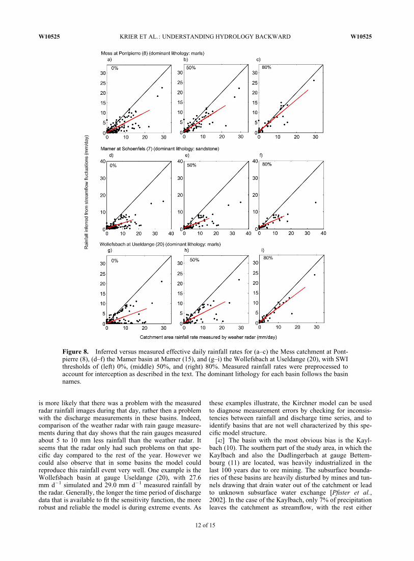
[39] Generally, we found better model performance inbasins with predominantly marly lithologies (e.g., the Mier-bech basin at gauge Huncherange (9) in Figure 7, the Messat gauge Pontpierre (8) and the Wollefsbach at gauge Usel-dange (20) in Figure 8). Marl is a sedimentary rock com-posed primarily of clay and calcium carbonate, and tends tobe impermeable. During periods of extended rainfall, soilsbecome saturated and connectivity between different soillayers is established, generating saturated overland flow andrapid subsurface flow. The Mess River (8) is located in thesouthern part of the Alzette catchment in a region noted forclay soils, which inhibit deep infiltration. Pfister et al. [2002]

Figure 6. Recession plots for the Schwebich river at Useldange (21) with SWI thresholds of 0%, 50%and 80%. The blue dots in Figures 6a, 6b, and 6c represent the time steps when P and E can be neglectedand the specific SWI threshold occurred. The black dots in Figures 6a–6f are the binned means.


10 of 15

showed that the maximum runoff coefficients (the percent-age of precipitation that appears as runoff), obtained via thedouble-mass curves of rainfall and runoff for 18 subcatch-ments of the Alzette catchment, range between 10% and66%. They defined a runoff coefficient of 54% for the MessRiver at gauge Pontpierre (8), which is close to the maxi-mum measured in the entire Alzette catchment. We arguethat this partly explains the good results obtained in that sub-basin using both the original Kirchner model and the modelwith higher SWI thresholds.

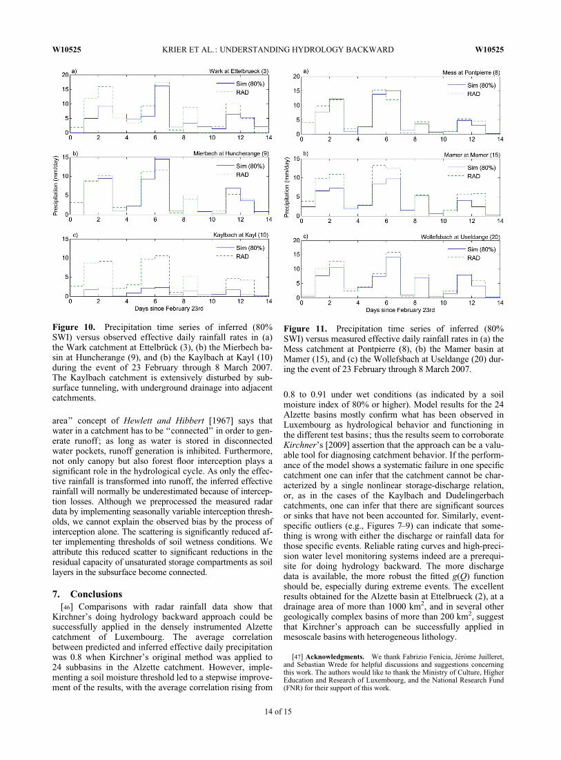
[40] Figures 10 and 11 show that during the rainfallevent after 23 February the timing of the predicted rainfallpeaks in the presented basins is very accurate. The Wollefs-bach basin at gauge Useldange (20) in Figure 11c showed

particularly good performance. Although the model greatlyunderestimated the rainfall intensities in the Kaylbach ba-sin (in Figure 10c; see further explanations below), the tim-ing in all examples of the event was exact.

[41] In Figure 9 we can observe error outliers in the boxplots with values up to 20 mm d�1. After analyzing theinput data it turned out that the errors around –20 mm d�1

for the basins with the IDs 7, 11, 15, and 23 all occurred onthe same day on 17 February. During that day the raingauges recorded the most intense rainfall event in the yearof our study, followed by the highest discharge peaks in allstreams. The weather radar measured rainfall intensities upto 40 mm d�1 in the Pall basin (18). Because similar errorsoccur in different basins at the same time, we argue that it

Figure 7. Inferred versus measured effective daily rainfall rates for (a–c) the Wark catchment atEttelbrück (3), (d–f) the Mierbech basin at Huncherange (9), and (g–i) the Kaylbach at Kayl (10), withSWI thresholds of (left) 0%, (middle) 50%, and (right) 80%. Measured rainfall rates were preprocessedto account for interception as described in the text. The Kaylbach catchment is extensively disturbed bysubsurface tunneling, with underground drainage into adjacent catchments. The dominant lithology foreach basin follows the basin names.


11 of 15

is more likely that there was a problem with the measuredradar rainfall images during that day, rather then a problemwith the discharge measurements in these basins. Indeed,comparison of the weather radar with rain gauge measure-ments during that day shows that the rain gauges measuredabout 5 to 10 mm less rainfall than the weather radar. Itseems that the radar only had such problems on that spe-cific day compared to the rest of the year. However wecould also observe that in some basins the model couldreproduce this rainfall event very well. One example is theWollefsbach basin at gauge Useldange (20), with 27.6mm d�1 simulated and 29.0 mm d�1 measured rainfall bythe radar. Generally, the longer the time period of dischargedata that is available to fit the sensitivity function, the morerobust and reliable the model is during extreme events. As

these examples illustrate, the Kirchner model can be usedto diagnose measurement errors by checking for inconsis-tencies between rainfall and discharge time series, and toidentify basins that are not well characterized by this spe-cific model structure.

[42] The basin with the most obvious bias is the Kayl-bach (10). The southern part of the study area, in which theKaylbach and also the Dudlingerbach at gauge Bettem-bourg (11) are located, was heavily industrialized in thelast 100 years due to ore mining. The subsurface bounda-ries of these basins are heavily disturbed by mines and tun-nels drawing that drain water out of the catchment or leadto unknown subsurface water exchange [Pfister et al.,2002]. In the case of the Kaylbach, only 7% of precipitationleaves the catchment as streamflow, with the rest either

Figure 8. Inferred versus measured effective daily rainfall rates for (a–c) the Mess catchment at Pont-pierre (8), (d–f) the Mamer basin at Mamer (15), and (g–i) the Wollefsbach at Useldange (20), with SWIthresholds of (left) 0%, (middle) 50%, and (right) 80%. Measured rainfall rates were preprocessed toaccount for interception as described in the text. The dominant lithology for each basin follows the basinnames.


12 of 15

evaporating or draining away through tunnels. This explainsthe significant underestimation of rainfall (see the Kaylbach(10) plots in Figures 7g–7i). We argue that the lower modelperformance in this case is not due to the limitations of themodel but rather to the disturbed water balance in thatcatchment.

[43] As already hypothesized by Kirchner [2009] the the-oretical foundations of the method are challenged by catch-ments with heterogeneous and complex geology, such asthose that have multiple unconnected subsurface reservoirswith dry patches in between. In such configurations dis-charge may not be a single-valued function of storage, butinstead may depend on how that storage is distributedamong various subsurface reservoirs, and thus streamflowfluctuations may not be unambiguously related to storagefluctuations. However, our results do not show a clear rela-tionship between model performance and the geologicalcomplexity of the individual catchments. For example, thePall catchment at gauge Niederpallen (18) is dominatedpartly by schist and partly by different types of marls, whichwould seem to make it difficult to characterize the basin asone simple dynamical system. Nonetheless, the performanceof the model is not markedly better or worse in the Pallcatchment than in the other catchments of the Alzette basin.Our results demonstrate rather good performance of the

model even in the most challenging catchment configura-tions. Likewise, the model performance in larger basins,with drainage areas between 200 and 1000 km2, is at leastas good, and possibly even better, than it is in basins withdrainage areas of 20 km2 or less. Considered together, theseresults suggest that once a critical soil moisture threshold isexceeded and the connectivity between multiple reservoirsis established the model performs reasonably well even in acomplex environment.

[44] Kirchner [2009] has pointed out that snowfall andmelting could potentially affect model results. One canexpect to obtain false pulses of inferred effective precipita-tion during periods of snowmelt and rain on snow with sub-sequent melt of the snowpack; what is inferred in suchcases is not precipitation per se (and particularly not frozenprecipitation), but rather wet precipitation (net of interceptionlosses) plus snowmelt. However, in the area under investiga-tion snowmelt-induced runoff does not occur very frequently,so this aspect of the model could not be investigated.

[45] At low rainfall rates some point scattering can stillbe observed in Figures 7a, 7d, 8d, 8g, and 8h, close to the xaxis, especially with a SWI threshold of 0%, even afterimplementing the interception storage. This scatter partlyresults from very low measured radar rainfall rates that didnot cause any reaction in the stream. The ‘‘variable source

Figure 9. Box plots of the prediction errors of the simulated daily rainfall rates. The blue box extendsfrom the lower to upper quartile values of the data, with a red line at the median. The black whiskersextend from the box to show the expected range of the data, estimated as 1.5 � (75%–25%). Green out-lier points are those past the ends of the whiskers.


13 of 15

area’’ concept of Hewlett and Hibbert [1967] says thatwater in a catchment has to be ‘‘connected’’ in order to gen-erate runoff; as long as water is stored in disconnectedwater pockets, runoff generation is inhibited. Furthermore,not only canopy but also forest floor interception plays asignificant role in the hydrological cycle. As only the effec-tive rainfall is transformed into runoff, the inferred effectiverainfall will normally be underestimated because of intercep-tion losses. Although we preprocessed the measured radardata by implementing seasonally variable interception thresh-olds, we cannot explain the observed bias by the process ofinterception alone. The scattering is significantly reduced af-ter implementing thresholds of soil wetness conditions. Weattribute this reduced scatter to significant reductions in theresidual capacity of unsaturated storage compartments as soillayers in the subsurface become connected.

7. Conclusions[46] Comparisons with radar rainfall data show that

Kirchner’s doing hydrology backward approach could besuccessfully applied in the densely instrumented Alzettecatchment of Luxembourg. The average correlationbetween predicted and inferred effective daily precipitationwas 0.8 when Kirchner’s original method was applied to24 subbasins in the Alzette catchment. However, imple-menting a soil moisture threshold led to a stepwise improve-ment of the results, with the average correlation rising from

0.8 to 0.91 under wet conditions (as indicated by a soilmoisture index of 80% or higher). Model results for the 24Alzette basins mostly confirm what has been observed inLuxembourg as hydrological behavior and functioning inthe different test basins; thus the results seem to corroborateKirchner’s [2009] assertion that the approach can be a valu-able tool for diagnosing catchment behavior. If the perform-ance of the model shows a systematic failure in one specificcatchment one can infer that the catchment cannot be char-acterized by a single nonlinear storage-discharge relation,or, as in the cases of the Kaylbach and Dudelingerbachcatchments, one can infer that there are significant sourcesor sinks that have not been accounted for. Similarly, event-specific outliers (e.g., Figures 7–9) can indicate that some-thing is wrong with either the discharge or rainfall data forthose specific events. Reliable rating curves and high-preci-sion water level monitoring systems indeed are a prerequi-site for doing hydrology backward. The more dischargedata is available, the more robust the fitted g(Q) functionshould be, especially during extreme events. The excellentresults obtained for the Alzette basin at Ettelbrueck (2), at adrainage area of more than 1000 km2, and in several othergeologically complex basins of more than 200 km2, suggestthat Kirchner’s approach can be successfully applied inmesoscale basins with heterogeneous lithology.

[47] Acknowledgments. We thank Fabrizio Fenicia, Jerome Juilleret,and Sebastian Wrede for helpful discussions and suggestions concerningthis work. The authors would like to thank the Ministry of Culture, HigherEducation and Research of Luxembourg, and the National Research Fund(FNR) for their support of this work.

Figure 10. Precipitation time series of inferred (80%SWI) versus observed effective daily rainfall rates in (a)the Wark catchment at Ettelbrück (3), (b) the Mierbech ba-sin at Huncherange (9), and (b) the Kaylbach at Kayl (10)during the event of 23 February through 8 March 2007.The Kaylbach catchment is extensively disturbed by sub-surface tunneling, with underground drainage into adjacentcatchments.

Figure 11. Precipitation time series of inferred (80%SWI) versus measured effective daily rainfall rates in (a) theMess catchment at Pontpierre (8), (b) the Mamer basin atMamer (15), and (c) the Wollefsbach at Useldange (20) dur-ing the event of 23 February through 8 March 2007.


14 of 15

ReferencesAnctil, F., L. Lauzon, and M. Filion (2008), Added gains of soil moisture

content observations for streamflow predictions using neural networks,J. Hydrol., 359(3–4), 225–234.

Aubert, D., C. Loumagne, and L. Oudin (2003), Sequential assimilation ofsoil moisture and streamflow data in a conceptual rainfall runoff model,J. Hydrol., 280, 145–161.

Bartels, H., E. Weigl, T. Reich, P. Lang, A. Wagner, O. Kohler, andN. Gerlach (2004), Routineverfahren zur Online-Aneichung der Radar-niederschlagsdaten mit Hilfe von automatischen Bodenniederschlagssta-tionen (Ombrometer), in Projekt RADOLAN, report, pp. 78–97, GermanWeather Serv., Offenbach, Germany.

Brocca, L., F. Melone, T. Moramarco, and V. P. Singh (2009), Assimilationof observed soil moisture data in storm rainfall-runoff modeling, J.Hydrol., Eng., 14(2), 153–165.

Brocca, L., F. Melone, T. Moramarco, W. Wagner, and S. Hasenauer (2010a),ASCAT soil wetness index validation through in-situ and modeled soilmoisture data in central Italy, Remote Sens. Environ., 114(11), 2745–2755.

Brocca, L., S. Hasenauer, P. de Rosnay, F. Melone, T. Moramarco, P. Matgen,J. Mart��nez-Fernandez, P. Llorens, J. Latron, and C. Martin (2010b), Con-sistent validation of H-SAF soil moisture satellite and model productsagainst ground measurements for selected sites in Europe, in AssociatedScientist Activity in the Framework of the Satellite Application Facility onSupport to Operational Hydrology and Water Management (H-SAF),report, 56 pp., H-SAF, Perugia, Italy.

Brocca, L., F. Melone, T. Moramarco, and R. Morbidelli (2010c), Spatial-temporal variability of soil moisture and its estimation across scales,Water Resour. Res., 46, W02516, doi:10.1029/2009WR008016.

Brutsaert, W. (1982), Evaporation Into the Atmosphere: Theory, History,and Applications, Kluwer Acad., Dordrecht, Netherlands.

Brutsaert, W., and J. L. Nieber (1977), Regionalized drought flow hydro-graphs from a mature glaciated plateau, Water Resour. Res., 13, 637–643, doi:10.1029/WR013i003p00637.

Daniel, J. F. (1976), Estimating groundwater evapotranspiration fromstreamflow records, Water Resour. Res., 12(3), 360–364.

Detty, J. M., and K. J. McGuire (2010), Threshold changes in storm runoffgeneration at a till-mantled headwater catchment, Water Resour. Res.,46, W07525, doi:10.1029/2009WR008102.

Federer, C. A. (1973), Forest transpiration greatly speeds streamflow reces-sion, Water Resour. Res., 9(6), 1599–1604.

Fenicia, F., H. H. G. Savenije, P. Matgen, and L. Pfister (2006), Is thegroundwater reservoir linear? Learning from data in hydrological model-ling, Hydrol. Earth Syst. Sci., 10, 139–150.

Gerrits, A. M. J., L. Pfister, and H. H. G. Savenije (2010), Spatial and tem-poral variability of canopy and forest floor interception in a beech forest,Hydrol. Processes, 24, 3011–3025, doi:10.1002/hyp.7712.

Goudenhoofdt, E., and L. Delobbe (2009), Evaluation of radar-gauge merg-ing methods for quantitative precipitation estimates, Hydrol. Earth Syst.Sci., 13, 195–203.

Graham, C. B., R. A. Woods, and J. J. McDonnell (2010), Hillslope thresh-old response to rainfall: (1) A field based forensic approach, J. Hydrol.,393, 65–76, doi:10.1016/j.jhydrol.2009.12.015.

Heitz, S., P. Matgen, S. Hasenauer, C. Hissler, L. Pfister, L. Hoffmann,and L. Wagner (2010), ASCAT-ENVISAT ASAR downscaled soilmoisture product: Soil wetness index retrieval over Luxembourg, paperpresented at the Living Planet Symposium, Eur. Space Agency, Bergen,Norway.

Hewlett, J. D., and A. R. Hibbert (1967), Factors affecting the response ofsmall watersheds to precipitation in humid areas, edited by W. E. Sopperand H. W. Lull, pp. 275–290, Pergamon Press, Oxford, UK.

Juilleret, J., F. Fenicia, P. Matgen, C. Tailliez, L. Hoffmann, and L. Pfister(2005), Soutien des debits d’etiage des cours d’eau du grand-duche duLuxembourg par l’aquifere du Gres du Luxemboug, in Proceedings ofthe 2nd International Conference on Sandstone Landscapes, Museenational d’histoire naturelle Luxembourg, Vianden, Luxembourg.

Kirchner, J. W. (2009), Catchments as simple dynamical systems: Catchmentcharacterization, rainfall-runoff modeling, and doing hydrology backward,Water Resour. Res., 45, W02429, doi:10.1029/2008WR006912.

Krein, A., M. Salvia-Castellvi, J.-F. Iffly, F. Barnich, P. Matgen, R. Vanden Bos, L. Hoffmann, L. Pfister, H. Hofmann, and A. Kies (2007), Uncer-tainty in chemical hydrograph separation, in Proceedings of the ERB2006 Conference on Uncertainties in the Monitoring-Conceptualisation-Modelling Sequence of Catchment Research, pp. 21–26, ERB, Paris.

Loew, A., and F. Schlenz (2011), A dynamic approach for evaluating coarsescale satellite soil moisture products, Hydrol. Earth Syst. Sci., 15, 75–90.

Matgen, P., S. Heitz, S. Hasenauer, C. Hissler, L. Brocca, L. Hoffmann, W.Wagner, and H. H. G. Savenije (2012), On the potential for METOPASCAT-derived soil wetness indices as a new aperture for hydrologicalmonitoring and prediction: A field evaluation over Luxembourg, Hydrol.Processes., 26, 2346–2359, doi:10.1002/hyp.8316.

Pfister, L., J.-F. Iffly, L. Hoffmann, and J. Humbert (2002), Use of regional-ized stormflow coefficients with a view to hydroclimatological hazardmapping, Hydrol. Sci. J., 47, 479–491.

Pfister, L., G. Drogue, A. El Idrissi, J.-F. Iffly, C. Poirier, and L. Hoffmann(2004), Spatial variability of trends in the rainfall-runoff relationship: Amesoscale study in the Mosel basin, Clim. Change, 66, 67–87, doi:10.1023/B:CLIM.0000043160.26398.4c.

Savenije, H. H. G. (2010), HESS opinions ‘‘Topography driven conceptualmodelling (FLEX-Topo),’’ Hydrol. Earth Syst. Sci. Discuss., 7, 4635–4656.

Sinclair, S., and G. Pegram (2005), Combining radar and rain gaugerainfall estimates using conditional merging, Atmos. Sci. Lett., 6, 19–22, doi:10.1002/asl.85.

Teuling, A. J., I. Lehner, J. W. Kirchner, and S. I. Seneviratne (2010), Catch-ments as simple dynamical systems: Experience from a Swiss prealpinecatchment, Water Resour. Res., 46, W10502, doi:10.1029/2009WR008777.

Tramblay, Y., C. Bouvier, C. Martin, J. F. Didon-Lescot, D. Todorovik, andJ. M. Domergue (2010), Assessment of initial soil moisture conditionsfor event-based rainfall-runoff modelling, J. Hydrol., 380(3–4), 305–317.

Uchida, T., J. J. McDonnell, and Y. Asano (2006), Functional intercompari-son of hillslopes and small catchments by examining water source, flow-path and mean residence time, J. Hydrol., 327, 627–642, doi:10.1016/j.jhydrol.2006.02.037.

Uhlenbrook, S. (2003), An empirical approach for delineating spatial unitswith the same dominating runoff generation processes, Phys. Chem.Earth, Parts A/B/C, 28, 297–303, doi:10.1016/S1474-7065(03)00041-X.

Vachaud, G. A., A. Passerat de Silans, P. Balabanis, and M. Vauclin(1985), Temporal stability of spatially measured soil water probabilitydensity function, Soil Sci. Soc. Am. J., 49, 822–828.

Young, P. C. (2006), Rainfall-Runoff Modeling: Transfer Function Models,John Wiley, Hoboken, N. J.

Zehe, E., and M. Sivapalan (2009), Threshold behaviour in hydrologicalsystems as (human) geo-ecosystems: Manifestations, controls, implica-tions, Hydrol. Earth Syst. Sci., 13, 1273–1297.

Zehe, E., H. Elsenbeer, F. Lindenmaier, K. Schulz, and G. Blöschl (2007),Patterns of predictability in hydrological threshold systems, WaterResour. Res., 43, W07434, doi:10.1029/2006WR005589.

Zehe, E., T. Graeff, M. Morgner, A. Bauer, and A. Bronstert (2010), Plotand field scale soil moisture dynamics and subsurface wetness control onrunoff generation in a headwater in the Ore mountains, Hydrol. EarthSystem Sci., 14, 873–889.


15 of 15

Inferring catchment precipitation by doing hydrology...

Documents

Transcript of Inferring catchment precipitation by doing hydrology...