Inferring Air Pollution by Sniffing Social Media

Shike Mei, Han Li, Jing Fan, Xiaojin Zhu and Charles R. DyerDepartment of Computer Sciences, University of Wisconsin-Madison, Madison, WI, USA 53706

{mei, hanli, fanj, jerryzhu, dyer}@cs.wisc.edu

Abstract—The first step to deal with the significant issue ofair pollution in China and elsewhere in the world is to monitorit. While more physical monitoring stations are built, currentcoverage is limited to large cities with most other places under-monitored. In this paper we propose a complementary approachto monitor Air Quality Index (AQI): using machine learningmodels to estimate AQI from social media posts. We propose aseries of progressively more sophisticated machine learning mod-els, culminating in a Markov Random Field model that utilizesthe text content in social media as well as the spatiotemporalcorrelation among cities and days. Our extensive experimentson Sina Weibo data from 108 cities during a one-month perioddemonstrate the accurate AQI prediction performance of ourapproach.

I. INTRODUCTION

Air pollution is a significant issue in China and elsewherearound the world. For example, in 2013 Beijing had 58 dayswhen the Air Quality Index (AQI) was higher than 200 or“heavy pollution.”1 In December 2013 the east and centralregions of China, which have more than 600 million people,experienced heavy pollution for more than two weeks. Airpollution is harmful to people’s health, causing “eye irritation,lung and throat irritation, lung cancer and problems with babiesat birth”2.

To better deal with the problems of air pollution, the firststep is to monitor air quality. From January 1 to November1, 2013, the coverage of physical monitoring stations hasincreased from 74 cities to 108 cities in China. Also, theChinese government has started to include PM2.5 (a majorand dangerous air pollutant) into AQI monitoring3.

The cost of establishing and maintaining physical moni-toring stations limits their deployment currently to large andmedium cities only. As a result, AQI monitoring in manyregions such as small cities and rural towns is still lacking.To help people in these regions obtain air quality information,we consider the following question: can we estimate AQIwithout physical monitoring by using other, already available,information sources?

In this paper we estimate AQI using social media dataas the information source. Social media is a rich and timelyinformation source about air pollution in China. The mostpopular social media site in China, Sina Weibo, has about 100million messages posted every day from all over the country4.Our key observation is that high AQI (poor air quality) in aregion causes more Weibo posts from that region to discuss

1http://www.cnemc.cn2http://www.cdc.gov/air/particulate matter.html3The PM2.5 information in China is reported at http://www.cnemc.cn4According to http://en.wikipedia.org/wiki/Sina Weibo

air pollution. For instance, here are some random Weibo posts(in Chinese) that contain the word “mai” ( , haze):

In fact, the word “mai” is positively correlated with AQIas shown in Figures 1(a,b). Figure 1(c) further visualizes thefrequency of some Chinese characters that co-occur with “mai”in Weibo posts.

Our main machine learning model is a Markov RandomField that exploits this and other correlations. This paperdemonstrates that our method can accurately estimate AQIfrom publicly-available Weibo posts, thereby offering an inex-pensive way to obtain information about air quality in diverseareas in China, not limited to cities with AQI monitoringstations.

We also point out the main limitations of our approachupfront. First, our model does not forecast future AQI butrather estimates current AQI from near-realtime populationreactions in social media. Second, our model is subject tothe availability of social media posts and therefore does notapply to remote regions with extremely low social media userpopulations. Still, this work provides complementary value toexisting AQI monitoring approaches, and can be an integralpart in the overall solution to the air pollution problem.

The present paper is related to a line of recent work thatattempts to gather air pollution information based on sourcesother than monitor stations. Honicky et al. [3] suggested col-lecting air pollution information by sensors attached to mobilephones. Poduri et al. [4] estimated the extent of airborneparticulate matter by commodity cameras that are commonlyused in mobile phones. Aoki et al. [1] used vehicles to monitorair quality by deploying mobile air quality sensing platformson street sweeping trucks in San Francisco. Recently, Zheng etal. [6] and Chen et al. [2] estimated the air quality in big citiesby fusing monitor stations data with meteorological and trafficdata. Our computational model is distinct and builds upon therecent work by Xu et al. [5], which monitored spatial-temporalsignals from social media. However, we focus on predicting airpollution from the text content in social media, whereas theyonly counted the number of wildlife roadkill event occurrencesin social media.

●

●

●

●

●

●

●

●

●●

●● ● ●

● ●

●

●

●

●

●

●

●

●

●● ●●

●

●●

0.00

000.

0010

0.00

200.

0030

Wor

d P

ropo

rtio

n of

'Mai

' 50 100 150 200 250 300 350

AQI

●

● ● ●●

●●● ●●

●●● ●

●

●

●

●

●

●

●

●

●

●

●●

● ●●●

●

0.00

00.

001

0.00

20.

003

0.00

40.

005

0.00

6

Wor

d P

ropo

rtio

n of

'Mai

'

50 100 150 200 250 300 350

AQI

(a) Beijing (b) Shanghai (c) word cloud (d) 108 monitoring citiesFig. 1: (a,b) Daily proportion of the word “mai” (haze) in Weibo posts vs. AQI in Beijing and Shanghai between November13 and December 12, 2013. The correlation coefficient ρ are 0.799 and 0.709 for Beijing and Shanghai, respectively. (c) Wordcloud showing the most frequent Chinese characters that occur in Weibo posts containing “mai,” produced using tagxedo.com.(d) The 108 cities with air quality monitor stations in China.

II. COLLECTION AND PROCESSING OF DATA

A. Data Collection

We collected posts to Sina Weibo from 108 cities (i.e., allcities with publicly available AQI data) in China during thetime period November 18 to December 18, 2013. The locationof the 108 cities is shown in Figure 1(a). The collection wasdone by calling the “nearby photos” API of Sina Weibo5.There are constraints: the API returns at most 200 posts; theposts’ GPS coordinates should lie within a 10-km radius circledefined by the center’s coordinates; and the time when theposts were posted should be in a specific one hour long period.We specified the center of the circles at each city’s geographiccenter found by Google Maps. Due to the limitation of the API,we collected at most 200 posts per hour per city. On average,we obtained about 1,380 posts in each spatiotemporal bin (cityand day).

We collected AQI information for these 108 cities everyhour from the Ministry of Environmental Protection of China6. These hourly data were averaged to produce a daily AQIvalue for each city. Table I shows the data distribution.

TABLE I: Distribution of spatiotemporal bins according to AQIAQI [0, 100) [100, 200) [200, 300) ≥ 300 All

Number of bins 1422 1313 397 185 3317Proportion of bins 42.87% 39.58% 11.96% 5.57% 100.00%

B. Text Processing

From each Weibo post we extracted the text informationcontained in the posts. First, we used the open-source Chinesesegmentation software ANSJ7 to segment the Chinese text ineach post. Each output segment in each post was regarded asa word. We filtered out all the stopwords using the stopwordlist at http://nlp.csai.tsinghua.edu.cn/thulac/. We created a vo-cabulary by removing all word types appearing less than 10times in the whole dataset. Our vocabulary contained 100,000word types. We aggregated all the posts in one (city, day) binas one “document.” Finally, we represented each document asa bag-of-words vector to be defined below.

5http://open.weibo.com/wiki/2/place/nearby/photos6http://113.108.142.147:20035/emcpublish/7https://github.com/ansjsun/

C. Evaluation

We first introduce our notation for the data. For spa-tiotemporal bin (s, t), the bag-of-words vector representing thepooled Weibo posts in that bin is denoted xs,t, and the dailyaverage AQI is denoted ys,t. For evaluation, we divided thecities as training cities Strain and test cities Stest. All bins(s, t) with s ∈ Strain form the training set. The other binsform the test set. Our goal is to estimate ys,t in the test setgiven the AQI and Weibo content in the training set, and theWeibo content in the test set.

In the rest of the paper we introduce a series of machinelearning methods for estimating AQI. The differences betweenthese methods will shed light on the merits of different featuresand spatiotemporal correlations in predicting air pollution. Tocompare different machine learning methods, we used meansquare error (MSE) between the predicted AQI ytests,t andthe actual AQI ytests,t to evaluate the performance: MSE =

1#TestDataPoints

∑s,t(y

tests,t − ytests,t )2.

III. AQI PREDICTION BASED ON “MAI”

A. The Models

To begin, we consider very simple regression models basedon only one feature: the proportion of the word “mai” in eachbin. This proportion is one element of xs,t and we denote itas xmais,t . This assumption captures the intuition that poor airquality (i.e., high ys,t values) will lead to more complaintsabout “mai” in social media, and is justified by Figures 1(a,b).

We consider two machine learning models: ridge regressionand support vector regression. Ridge regression learns theslope β1 and the offset β0 by solving the following opti-mization problem on the training set, argminβ0,β1

12

∑s,t(ys,t−

β1xmais,t − β0)2 + C

2 (β20 + β2

1), where C is the regularizationparameter to trade off between training loss and model com-plexity. Letting zs,t = [1, xmais,t ] and β = [β0, β1], then theproblem has the standard notation:

argminβ1

2

∑s,t

(ys,t − βT zs,t)2 +

C

2‖β‖22. (1)

Another commonly used linear regression model is supportvector regression (SVR). It solves the following constrained

TABLE II: Prediction performance with only one feature,“mai”

AQI [0, 100] (100, 200] (200, 300] (300, 1000) AllMSE for Ridge Regression 4739± 74 15494± 167 38562± 677 65048± 1601 17032± 470

MSE for SVR 4718± 23 16511± 130 40791± 511 68485± 1880 17914± 430

optimization problem,

argminβ

1

2‖β‖22 + CSV R

∑s,t

ξs,t

s.t. |ys,t − βT zs,t| ≤ ε+ ξs,t; ξs,t ≥ 0 (2)

where CSV R is a regularization parameter and ε is the toler-ance of error.

B. Experimental Results

We randomly divided the 108 cities into a training set with80 cities and a test set with 27 cities. The parameter C, CSV Rand ε were tuned using 5-fold cross-validation (CV) and thebest values were C = 106, CSV R = 105 and ε = 10−2. Theaverage test MSEs of five runs on random train/test splits areshown in Table II. the overall prediction MSE is large (a MSEaround 17000 translates to roughly off by 130 in AQI value).Therefore, prediction based on only the most intuitive featureis not enough. We need to utilize more information, as weexplain in the next sections.

IV. AQI PREDICTION USING FULL BOW FEATURES

A. The Models

We generalize the above methods as regression based on allWeibo bag-of-words features (with dimensionality 100,000).The same ridge regression and SVR as in Eq (1) and Eq (2)are used except for higher dimensional parameter vectors. Were-tuned the parameters with cross-validation.

B. Experimental Results

The experiment settings were exactly the same as inSection III-B. The best parameter settings tuned by 5-fold CVwere C = 103, CSV R = 103 and ε = 10−2.

Table IV shows the results. The prediction performanceusing the full BOW vector is much better than predictionbased on only “mai”. The overall MSE reduces to about3500, which roughly translates to AQI error of less than 60.For spatiotemporal bins with AQI< 200 (“light pollution” 8),the prediction has MSE less than 2300 (AQI error less than50). For bins with AQI> 300 (“severely polluted”), the AQIprediction is off by no more than 150 on average. So itusually does not predict a severely polluted day as good airquality (with AQI ≤ 100). As before, the MSEs of ridgeregression and SVR are similar. Therefore, the problem is notvery sensitive to the specific form of training loss (hinge lossin SVR or L2 norm in ridge regression).

We are also interested in the words with the largest absolutevalue of weights (i.e., top words). First, we removed thetop words which are city names because they are not easilyinterpretable. Then, the words with the largest positive weights

8The definition of AQI levels can be found in http://en.wikipedia.org/wiki/Air quality index

and the smallest negative weights learned in ridge regressionare shown9 in Table III. The words with the largest positiveweights are all strongly indicative of poor air quality. Thewords with the smallest negative weights are indicative of goodweather and perhaps cold fronts which sweep air pollutionaway. Therefore, our regression utilizes the Weibo contentstrongly related with air quality to estimate the AQI accurately.

TABLE III: Features with extreme weightsChinese word English translation weight霾 haze 12496

污染 pollution 8865

室内 indoor 5562

严重 heavy 5501

停留 stay 5396

指数 index 5214... ... ...阳光 sunshine −4181晴 sunny −5087冷 cold −5715

Even though these prediction models are much improved,they only perform estimation on each spatiotemporal bin inisolation. We also want to know if the performance could beimproved by considering the spatial correlation of the cities.After all, air pollution occurs in large pockets that often spanseveral nearby cities. This will be investigated next.

TABLE IV: Prediction performance with the full BOW vectorAQI [0, 100] (100, 200] (200, 300] (300, 1000) All

MSE for Ridge Regression 2231± 97 1101± 25 6990± 281 22904± 929 3469± 121MSE for SVR 1705± 58 1291± 47 8275± 313 25772± 868 3598± 141

TABLE V: Prediction performance with KNNAQI [0, 100] (100, 200] (200, 300] (300, 1000) All

MSE for KNN 1336± 108 1910± 104 4396± 204 12607± 620 2646± 75

TABLE VI: Prediction performance with MRFAQI [0, 100] (100, 200] (200, 300] (300, 1000) All

MSE for MRF 1534± 96 1150± 77 3878± 231 11710± 782 2312± 105

V. AQI PREDICTION BY KNN

A. The Model

To exploit the spatial correlation among cities, we startwith a method that uses only nearby cities’ AQI information:k-nearest-neighbor (KNN) method. In KNN, the AQI of a testdata point ytests,t is predicted by the average of AQIs in thenearest K training cities (denoted as KNNtrain(s)) in the same

day t. That is, ytests,t =

∑s′∈KNNtrain

(s)ytrains′,t

K . The distancebetween cities is the straight-line distance. Note that this KNNdoes not use any social media information.

B. Experimental Results

We first tuned the number of nearest neighbors K, by 5-fold CV. The CV MSE for different values of K from 1 to 64

9We report that similar phenomenon is observed for SVR.

and the MSE is the smallest when K = 3. This K potentiallysuggests the characteristic size of a pollution pocket. With K =3, the test set MSE is shown in Table V. The KNN predictionis surprisingly good, considering that it does not utilize anyWeibo content. This is an important observation. It suggeststhat there can be synergy between spatial correlation and textcontent, which we explore in the next section.

We point out that the earlier linear regression models arestill valuable despite their slightly inferior MSE performance.KNN cannot predict anything without knowing the nearbycities’ AQI, whereas our linear regression models can predictAQI based on a completely separate information source: Weibotext. When there are no nearby cities with AQI information, orshould the AQI information become unavailable in the futurefor any reason, the linear regression models still work.

VI. MARKOV RANDOM FIELD FOR AQI ESTIMATION

A. The Model

The KNN results show the strength of spatial correlationand the regression model shows the power of Weibo content.Combining them together may further improve performance.Therefore, we now consider both in a Markov Random Field(MRF) model to model the correlation between AQI ys,t andsocial media information xs,t. As in linear regression, weassume that ys,t is related to the dot product between someweight β and xs,t, plus Gaussian noise ε with zero mean andσ2 variance ys,t ≈ β>xs,t+ε where ε ∼ N (0, σ2). We alsoassume that the weight β is drawn from a Gaussian distributionwith 0 mean and covariance σ2

βI: β ∼ N (0, σ2βI). This leads

to a log potential term in the MRF:

φ(y,X,β) ,∑s,t

(ys,t − βTxs,t)2

2σ2+‖β‖222σ2

β

. (3)

To take into account the spatial correlation between cities andthe temporal correlation within the same city, we define thepotential term between two spatiotemporal bins φ(ys,t, ys′,t′).For AQI values on the same day t, nearby cities shouldhave similar AQI. Therefore, we define KNN(s) as the setof K nearest neighbors of city s measured by geographicaldistance. And we define two cities s, s′ as similar, denoted ass ∼ s′, when s ∈ KNN(s′) or s′ ∈ KNN(s). Then we defineφ(ys,t, ys′,t) as φ(ys,t, ys′,t) = 1

2αSI(s′ ∼ s)(ys,t − ys′,t)2,

where I() is an indicator function and αS controls the strengthof spatial correlation (tuned using cross validation).

The AQI in the same city s on two adjacent days may alsohave similar values. We denote two days t and t′ as neighborst ∼ t′ when |t−t′| = 1. We model this by defining φ(ys,t, ys,t′)as φ(ys,t, ys,t′) = 1

2αT I(t′ ∼ t)(ys,t−ys,t′)2. αT controls the

temporal correlation. It is also tuned using cross validation. Insummary, the potentials φ(ys,t, ys′,t′) defined as

φ(ys,t, ys′,t′) =

12αS(ys,t − ys′,t′)

2 if t = t′, s′ ∼ s12αT (ys,t − ys′,t′)

2 if s = s′, t′ ∼ t0 otherwise

form an undirected graph among the y’s.

Summing up the potential functions in Eqs. (3) and (4),we get an MRF model that accounts for both spatiotemporal

correlations and social media. The joint probability is

p(y,X,β|σβ , σ, αS , αT )

∝ exp

−(φ(y,X,β) +∑s,t

∑s′,t′

φ(ys,t, ys′,t′))

. (4)

When αS = αT = 0, the MRF only considers the correlationbetween ys,t and xs,t. When σ = ∞, the MRF degeneratesto model only the spatiotemporal correlation. Therefore, ourMRF model combines both information.

B. Inference with the MRF

To perform inference using the MRF, all Weibo content Xis observable, the AQI values are divided into a training setytrain (observable) and a test set ytest (hidden), and the goal isto compute the MLE of p(β,ytest|X,ytrain, σW , σ, αS , αT ).According to Eq (4), that is

{β, ytest} = argminβ,ytest

∑s,t

(ys,t − βTxs,t)2

2σ2+‖β‖222σ2

β

+∑s,t

∑s′,t′

φ(ys,t, ys′,t′)). (5)

We can scale the terms so that σ = 1 withoutchanging the solution. Then the problem be-comes argminβ,ytest

∑s,t

(ys,t−βTxs,t)2

2 +‖β‖222σ2

β+∑

s,t

∑s′,t′ φ(ys,t, ys′,t′)). This optimization problem

is nonconvex. Our strategy is to alternately optimizeβ and ytest while keeping the other fixed, as follows.Given ytest, the optimization problem for β isargminβ

∑s,t

(ys,t−βTxs,t)2

2 +‖β‖222σ2

β. This is a ridge regression

problem where C = 1σ2β

is the regularization parameter thattrades-off the predictive error and the complexity of themodel. This problem can be solved in closed form as

β = (XTX+ CI)−1XTy. (6)

Optimizing ytest given β can be formulated asargmaxytest

∑s,t

(ytests,t −βTxs,t)

2

2 +∑s∼s′

∑t12αS(y

tests,t −

ytrains′,t )2 + 12

∑s,t αT (y

tests,t − ytests,t+1)

2. Letting thegradient zero, we obtain the system of equations forytest: (I + A)ytest = b, where b is a vector with

bs,t =αS

∑s′∼s,s′∈train y

trains′,t +βTxs,t

αS

∑s′∼s,s′∈train 1+1 , and A is a matrix with

the element at row (s,t) and column (s’,t’) defined as

as,t,s′,t′ =

−αS if s ∼ s′, t = t′∑s∼s αS +

∑t∼t αT if s = s′, t = t′

−αT if s = s′, t ∼ t′.

The optimal ytest is given by

ytest = (I +A)−1b. (7)

In summary, the inference algorithm is in Algorithm 1.

●● ● ● ●

●●

●

● ●

●

●● ●

●

●

●

●●

●●

● ●

●

●● ●

●

● ●●

●● ● ● ●

●●

●

● ●

●

●● ●

●

●

●

●●

●●

● ●

●

●● ●

●

● ●●

010

020

030

040

050

0

AQ

I

0 5 10 15 20 25 30

Date

● PredictedActual

●

●

●

●

●

●●

●

●

● ●

● ●

●

●

●

●

●

●

●

●

●

●

●●

●●

●

●

●●

●

●

●

●

●

●●

●

●

● ●

● ●

●

●

●

●

●

●

●

●

●

●

●●

●●

●

●

●●

010

020

030

040

050

0

AQ

I

0 5 10 15 20 25 30

Date

● PredictedActual

●

●

●

●

● ●

●

●

●●

●

●

●

●

●

●

●

●

●

●

●

●

●

● ●

●

●●

●

●●

●

●

●

●

● ●

●

●

●●

●

●

●

●

●

●

●

●

●

●

●

●

●

● ●

●

●●

●

●●

010

020

030

040

050

0

AQ

I

0 5 10 15 20 25 30

Date

● PredictedActual

● ●

●

●

●

●

●

●●

●

● ●

●

●

●

●

●

●●

●

●

●

●● ●

●● ●

●

●

●

● ●

●

●

●

●

●

●●

●

● ●

●

●

●

●

●

●●

●

●

●

●● ●

●● ●

●

●

●

010

020

030

040

050

0

AQ

I

0 5 10 15 20 25 30

Date

● PredictedActual

●

● ●

●

● ●

●

●

●

● ●●

●● ●

●

●

● ●

●

●

●●

●

● ●

● ●

●

●

●

●

● ●

●

● ●

●

●

●

● ●●

●● ●

●

●

● ●

●

●

●●

●

● ●

● ●

●

●

●

010

020

030

040

050

0

AQ

I

0 5 10 15 20 25 30

Date

● PredictedActual

(a) Fuzhou (b) Hangzhou (c) Ningbo (d) Jinhua (e) Shenyang

●

●

●

●

●

●●

●●

●

●

●

●

●●

●

●

●●

●

●

●

●●

●

●

●

●●

● ●●

●

●

●

●

●●

●●

●

●

●

●

●●

●

●

●●

●

●

●

●●

●

●

●

●●

● ●

010

020

030

040

050

0

AQ

I

0 5 10 15 20 25 30

Date

● PredictedActual

●

●

●

●

●

●

●

●

●

●●

●

●● ●

●●

●

●

●

●

●

●

● ●●

●

●

●

●

●

●

●

●

●

●

●

●

●

●

●●

●

●● ●

●●

●

●

●

●

●

●

● ●●

●

●

●

●

●

010

020

030

040

050

0

AQ

I

0 5 10 15 20 25 30

Date

● PredictedActual

●●

●

● ●

●

●

● ● ●

●

●●

● ●

●

● ●●

●

●

● ● ● ●

●

●

●

●

●

●

●●

●

● ●

●

●

● ● ●

●

●●

● ●

●

● ●●

●

●

● ● ● ●

●

●

●

●

●

●

010

020

030

040

050

0

AQ

I

0 5 10 15 20 25 30

Date

● PredictedActual

●●

●

●

●

●

●

●

● ●

●●

●

●

●●

●

● ●

●●

●

● ●

●

● ●●

●

●●

●●

●

●

●

●

●

●

● ●

●●

●

●

●●

●

● ●

●●

●

● ●

●

● ●●

●

●●

010

020

030

040

050

0

AQ

I

0 5 10 15 20 25 30

Date

● PredictedActual

●

●

●

●

● ●

● ●●

●

●●

●●

●●

● ● ●●

●●

● ●

●

●●

●

●●

●

●

●

●

●

● ●

● ●●

●

●●

●●

●●

● ● ●●

●●

● ●

●

●●

●

●●

●

010

020

030

040

050

0

AQ

I

0 5 10 15 20 25 30

Date

● PredictedActual

(f) Taiyuan (g) Tianjin (h) Xian (i) Zhuzhou (j) Beihai

●

●● ●

●

●

● ●

●

●

●

●

● ●

● ●

●

●

●

●

●

●

●●

●

●

●

●

●

●

●

●

●● ●

●

●

● ●

●

●

●

●

● ●

● ●

●

●

●

●

●

●

●●

●

●

●

●

●

●

●

010

020

030

040

050

0

AQ

I

0 5 10 15 20 25 30

Date

● PredictedActual

●●

●●

●

●●

●

● ●●

●

●

●

●

●

●●

●

●●

●● ●

●

●

●

●●

●●

●●

●●

●

●●

●

● ●●

●

●

●

●

●

●●

●

●●

●● ●

●

●

●

●●

●●

010

020

030

040

050

0

AQ

I

0 5 10 15 20 25 30

Date

● PredictedActual

●

●

●● ● ● ●

● ● ●●

●

● ●●

●

●

● ●

●

● ●●

● ●

●

●

●

●

● ●

●

●

●● ● ● ●

● ● ●●

●

● ●●

●

●

● ●

●

● ●●

● ●

●

●

●

●

● ●

010

020

030

040

050

0

AQ

I

0 5 10 15 20 25 30

Date

● PredictedActual

●●

●

●

●

●

●

●

●

●

●●

●

●

●

●

●

●

●

●

●

●

●● ●

●

●

●

●

● ●●●

●

●

●

●

●

●

●

●

●●

●

●

●

●

●

●

●

●

●

●

●● ●

●

●

●

●

● ●

010

020

030

040

050

0

AQ

I

0 5 10 15 20 25 30

Date

● PredictedActual

●

●

●

●

●

●

●

●

●

●

●

●

●

●

●

●

●

●

●

●

●

●

●●

●

●

●●

●

●

●●

●

●

●

●

●

●

●

●

●

●

●

●

●

●

●

●

●

●

●

●

●

●●

●

●

●●

●

●

●

010

020

030

040

050

0

AQ

I

0 5 10 15 20 25 30

Date

● PredictedActual

(k) Xiangyang (l) Xining (m) Shaoguan (n) Yangzhou (o) ZhengzhouFig. 3: Predicted AQI and actual AQI for 15 test cities from November 18 to December 18, 2013

●

●●

●

●

●

●

●

1000

2000

3000

4000

5000

6000

7000

Cro

ss V

alid

atio

n M

SE

1 2 3 4 8 16 32 64

K

●

●●

●

●

●

●

●

● MRF

(a) CV for K

●● ●

●

●

●

●

●

● ● ●

1000

2000

3000

4000

5000

6000

7000

Cro

ss V

alid

atio

n M

SE

1e−05 0.001 0.1 1 10 1000 1e+05σβ

2

●● ●

●

●

●

●

●

● ● ●

● MRF

(b) CV for σ2β

●

●

●● ●

●● ●

1000

2000

3000

4000

5000

6000

7000

Cro

ss V

alid

atio

n M

SE

0.01 0.1 0.2 0.5 1 2 4 8αS

●

●

●● ●

●● ●

● MRF

(c) CV for αS

● ● ● ● ● ● ●

●

●

●

●

●

1000

2000

3000

4000

5000

6000

7000

Cro

ss V

alid

atio

n M

SE

1e−06 1e−04 0.01 0.1 1 4αT

● ● ● ● ● ● ●

●

●

●

●

●

● MRF

(d) CV for αT

Fig. 2: Average MSE of folds in CV for four parameters

C. Cross Validation

In our MRF model we have five parameters: the numberof iterations T , the number of neighbors K, the variance ofthe Gaussian prior σ2

β, the strength of spatial correlation αS ,and the strength of temporal correlation αT . For computationalefficiency, we simply set T = 1. That is, we only do oneiteretion in the above algorithm. The other four parametersare tuned by 5-fold CV. The tuning curve of each parameterwith the other parameters fixed at their best values is in

Algorithm 1 Inference for MRF

Require: X, ytrain, σβ , σ, αS , αT and Tytest ⇐ 0for i = 1 to T do

update β using Eq (6)update ytest using Eq (7)

end forreturn β, ytest

Figures 2(a)–2(d). The best parameters are K = 3, σ2β = 10−3,

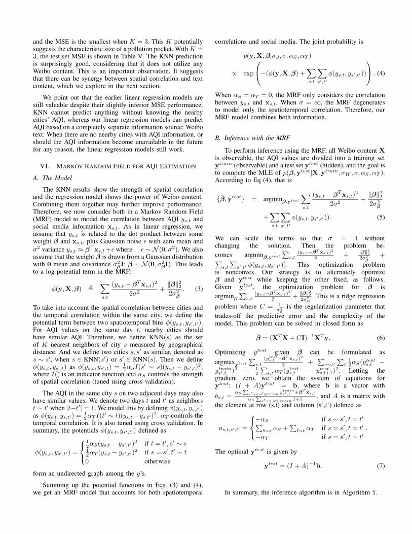
αS = 0.5 and αT = 0.0. Note that αT = 0.0 means thatexploiting temporal correlation does not help improve theprediction performance. This may due to that the temporal unit(a whole day) is large compared to the time scale of typicalAQI fluctuations. For exact AQI prediction, the fluctuationsbetween days are too large (see Figure 3).

D. Experimental Results on the Test Set

We show the MRF’s MSE on the test set in Table VI. Theoverall MSE is 2312, which is the best among the machinelearning models we considered. Therefore, combining Weibocontent and spatiotemporal correlation together improves per-formance. For the (city, day) bins with no heavy pollution(AQI< 200), the predictions do not deviate more than 40 (onaverage). Therefore, our method rarely make false heavy airpollution predictions on good air quality days. For the binswith severe pollution (AQI> 300), our predictions of AQIdeviate no more than 110 (on average). So we seldom makefalse negative predictions. The errors for high AQI days arelarger than the errors for lower AQI days because the training

data with high AQI (days with bad air quality) is fewer thanthe data with low AQI (days with good air quality).

To visualize our MRF model’s predictions, we randomlyselected 15 different cities from the test sets of five runs. Weshow the prediction AQI curves and the actual AQI curvesfrom 11/18/2013 to 12/18/2013 in Figure 3. Our predicted AQIcurves are close to the actual curves. Occasionally, on severelypolluted days (AQI> 300) the predictions are lower than theactual values. However, even in this case our prediction is stilluseful in that it predicts all of them as heavily polluted days(AQI> 200). We also point out the similarity between that theactual AQI curves in three nearby cities Hangzhou, Ningbo,and Jinhua (see Figure 3(b), Figure 3(c) and Figure 3(d)), afact that we exploited using spatial correlation potentials in ourMRF. However, another nearby city, Yangzhou, in Figure 3(n)does not has similar AQI with Hangzhou. This shows thatsmall cities’ AQI information cannot always be predicted bytheir nearby big cities. The AQI can be influenced by manyfactors, not only geographical distance.

●

●

●

●●

●●

●

●

●

● ● ●●

●

●●

●

●●

● ●

●●

●

●

● ●●

●

●

●

●●

●●

●

●

●

● ● ●●

●

●●

●

●●

● ●

●●

●

●

● ●●

010

020

030

040

050

0

AQ

I

0 5 10 15 20 25 30

Date

● Predicted

●

●

●

●●

●

●

●●

●

●

●

● ●

●

●●

●

●

●● ● ●

●●

●

● ●●

●

●

●

●●

●

●

●●

●

●

●

● ●

●

●●

●

●

●● ● ●

●●

●

● ●●

010

020

030

040

050

0

AQ

I

0 5 10 15 20 25 30

Date

● Predicted

● ●

●

●

●

●

● ●●

●

● ●

● ●

●

●

●

●

●●

●●

● ●

●

●●

●

●

● ●

●

●

●

●

● ●●

●

● ●

● ●

●

●

●

●

●●

●●

● ●

●

●●

●

●

010

020

030

040

050

0

AQ

I

0 5 10 15 20 25 30

Date

● Predicted

(a) Luoyang (b) Zhuji (c) Guilin

●

●

●●

●●

● ●●

●

●

●

●

●

● ● ●

●

●

●

●●

●

●

●

●

●

●

●

●

●

●●

●●

● ●●

●

●

●

●

●

● ● ●

●

●

●

●●

●

●

●

●

●

●

●

010

020

030

040

050

0

AQ

I

0 5 10 15 20 25 30

Date

● Predicted

●

●

●

●

●● ● ●

●

●

●

●

● ●

●

●● ●

●

● ● ●

●

● ● ●

●●

●

●

●

●

●

●● ● ●

●

●

●

●

● ●

●

●● ●

●

● ● ●

●

● ● ●

●●

●

010

020

030

040

050

0

AQ

I

0 5 10 15 20 25 30

Date

● Predicted

●

●

●

●

●

●

●

● ●

●

●

●

●

●●

●

●

●● ●

●

●●

● ●

● ●

●

●

●

●

●

●

●

●

●

● ●

●

●

●

●

●●

●

●

●● ●

●

●●

● ●

● ●

●

●

010

020

030

040

050

0

AQ

I

0 5 10 15 20 25 30

Date

● Predicted

(d) Dunhuang (e) Lijiang (f) Dali

Fig. 4: Predicted AQI for several cities with no official AQIinformation.

E. Out-of-Sample Predictions on Cities Without AQI Monitor-ing Stations

To demonstrate that our method can help predict the airquality in places without AQI monitoring stations, we usedour MRF model to predict the AQI for 26 additional citiesthat currently lack official air quality monitoring. The Weibodata collection and processing procedure was identical to thatin Section II except that the study period of this dataset wasfrom 01/17/2014 to 02/14/2014, which is after and does notoverlap with the 108-city study.

We show the predicted AQI curves for several such cities inFigure 4. Because there is no official public AQI informationon these 26 cities, we cannot judge our model prediction bycomparing it with the true AQI. However, we are able togive some indirect evidence to justify our predictions. First,Figures 4(a)–4(c) all have a peak AQI value near the middleof the study period (the 15th day or 16th day). We notethat the 15th day in the study period is Chinese new year’seve. Traditionally, people on this day celebrate with fireworks,

which usually emit a lot of air pollutants. We hypothesize thatthe peak AQI may be attributed to these fireworks emissions.The Chinese Ministry of Environmental Protection proclaimedheavy pollution on that day because of fireworks in almostall major cities, which supports our hypothesis10. Also, thepredicted AQI for Dunhuang increased during the 25th–29thdays in the study period (see Figure 4(d)). According to newsreports, Dunhuang had a dust storm in 2014 during that period,which probably contributed to the air pollution11. Finally, theair quality in Lijiang (see Figure 4(e)) looks much better thanother cities. This is consistent with the impression that Lijiangis a tourist destination with good air quality.

VII. DISCUSSION

We presented several estimators for air quality based onWeibo text content and spatiotemporal correlation betweencities. Our methods complement physical AQI monitoring bymonitoring stations. They may be particularly attractive forregions without monitoring stations. Our information sourceis inexpensively crawled from social media.

Our MRF model can easily combine other informationsources, including the topography of the areas and the weather.Particularly interesting are the photos users post to social me-dia. For future work, we may exploit the different behaviors ofpeople from large cities and small cities on the social networks.Also, different cultures in different regions in China may beconsidered. We are also interested in predicting AQI, whichdepends heavily on human activities and weather. Weather canalways be predicted. Therefore, understanding the pattern ofhuman activities by social media may help predicting AQI.

ACKNOWLEDGMENT

This work was supported in part by National ScienceFoundation grant IIS-1148012.

REFERENCES

[1] Paul M Aoki, RJ Honicky, Alan Mainwaring, Chris Myers, Eric Paulos,Sushmita Subramanian, and Allison Woodruff. A vehicle for research:using street sweepers to explore the landscape of environmental com-munity action. In Proceedings of the SIGCHI Conference on HumanFactors in Computing Systems, pages 375–384. ACM, 2009.

[2] Jiaoyan Chen, Huajun Chen, Guozhou Zheng, Jeff Z Pan, Honghan Wu,and Ningyu Zhang. Big smog meets web science: Smog disaster analysisbased on social media and device data on the web. In Proceedings ofthe 23th International World Wide Web Conference, 2014.

[3] Richard Honicky, Eric A Brewer, Eric Paulos, and Richard White. N-smarts: networked suite of mobile atmospheric real-time sensors. InProceedings of the Second ACM SIGCOMM Workshop on NetworkedSystems for Developing Regions, pages 25–30. ACM, 2008.

[4] Sameera Poduri, Anoop Nimkar, and Gaurav S Sukhatme. Visibilitymonitoring using mobile phones. Annual Report: Center for EmbeddedNetworked Sensing, pages 125–127, 2010.

[5] Jun-Ming Xu, Aniruddha Bhargava, Robert Nowak, and Xiaojin Zhu.Socioscope: Spatio-temporal signal recovery from social media. In Ma-chine Learning and Knowledge Discovery in Databases (ECML/PKDD),pages 644–659. Springer, 2012.

[6] Yu Zheng, Furui Liu, and Hsun-Ping Hsieh. U-air: When urban airquality inference meets big data. In Proceedings of the 19th ACMSIGKDD international conference on Knowledge discovery and datamining, pages 1436–1444. ACM, 2013.

10http://www.mep.gov.cn/gkml/hbb/qt/201401/t20140131 267406.htm11http://gansu.gansudaily.com.cn/system/2014/03/20/014933184.shtml