1

1

Inferential Statistics: A Frequentist Perspective

Mark A. Weaver, PhDFamily Health International

Office of AIDS Research, NIHICSSC, FHI

Goa, India, September 2009

2

2

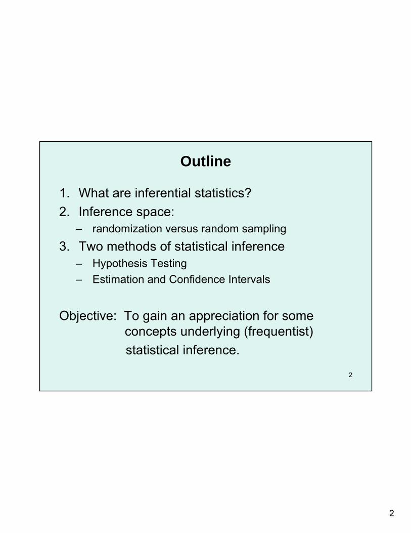
Outline

1. What are inferential statistics?2. Inference space:

– randomization versus random sampling3. Two methods of statistical inference

– Hypothesis Testing– Estimation and Confidence Intervals

Objective: To gain an appreciation for some concepts underlying (frequentist) statistical inference.

3

3

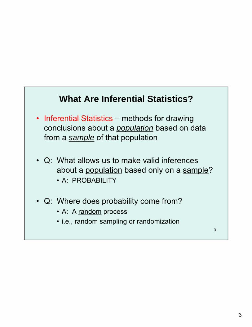
What Are Inferential Statistics?

• Inferential Statistics – methods for drawing conclusions about a population based on data from a sample of that population

• Q: What allows us to make valid inferences about a population based only on a sample?• A: PROBABILITY

• Q: Where does probability come from?• A: A random process• i.e., random sampling or randomization

4

4

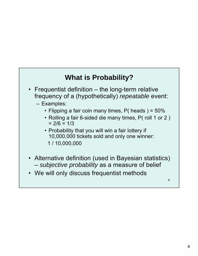
What is Probability?• Frequentist definition – the long-term relative

frequency of a (hypothetically) repeatable event:– Examples:

• Flipping a fair coin many times, P( heads ) = 50%• Rolling a fair 6-sided die many times, P( roll 1 or 2 )

= 2/6 = 1/3• Probability that you will win a fair lottery if

10,000,000 tickets sold and only one winner: 1 / 10,000,000

• Alternative definition (used in Bayesian statistics) – subjective probability as a measure of belief

• We will only discuss frequentist methods

5

5

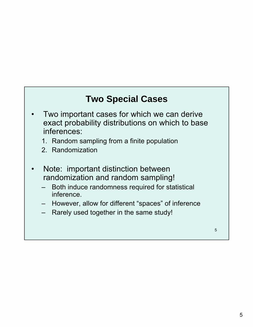
Two Special Cases• Two important cases for which we can derive

exact probability distributions on which to base inferences:1. Random sampling from a finite population2. Randomization

• Note: important distinction between randomization and random sampling!– Both induce randomness required for statistical

inference.– However, allow for different “spaces” of inference– Rarely used together in the same study!

6

6

Random Sampling from a Finite Population

• Consider a large, but finite, population of size N– Assume that the population is well-defined such that

we could (theoretically) list every member– We want to determine something about that

population• We take a sample of size n < N

– Using some random sampling method

7

7

Random Sampling from a Finite Population

• In theory, we could list all possible samples of size n• Thus, we could compute selection probability for any

individual in population simply by counting• In SRS, it is easy to show that the selection

probability for any individual is n / N

• Sampling inference in a nut shell:– selection probability can be used to “up-weight” each

individual’s contribution to the sample to estimate number of similar individuals in the population

8

8

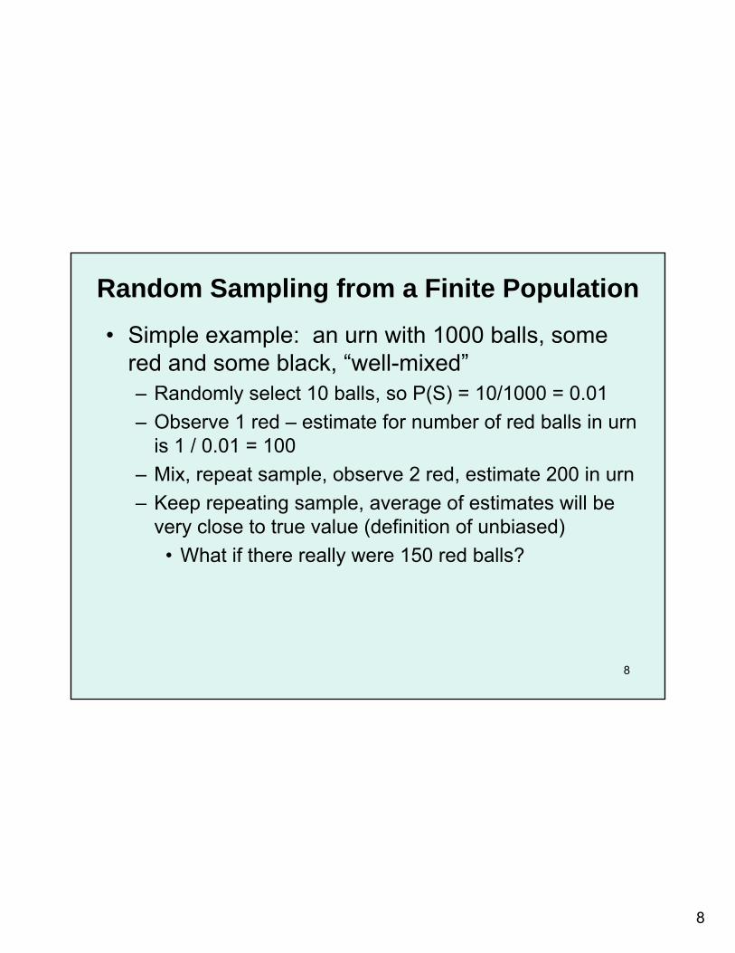
Random Sampling from a Finite Population• Simple example: an urn with 1000 balls, some

red and some black, “well-mixed”– Randomly select 10 balls, so P(S) = 10/1000 = 0.01– Observe 1 red – estimate for number of red balls in urn

is 1 / 0.01 = 100– Mix, repeat sample, observe 2 red, estimate 200 in urn– Keep repeating sample, average of estimates will be

very close to true value (definition of unbiased)• What if there really were 150 red balls?

9

9

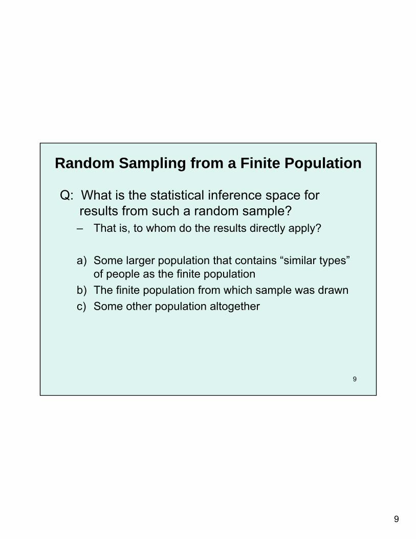
Random Sampling from a Finite Population

Q: What is the statistical inference space for results from such a random sample?– That is, to whom do the results directly apply?

a) Some larger population that contains “similar types”of people as the finite population

b) The finite population from which sample was drawnc) Some other population altogether

10

10

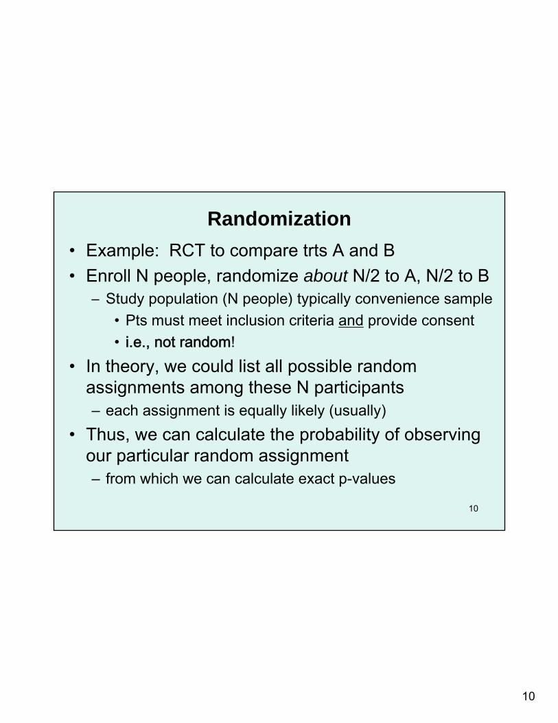
Randomization• Example: RCT to compare trts A and B• Enroll N people, randomize about N/2 to A, N/2 to B

– Study population (N people) typically convenience sample• Pts must meet inclusion criteria and provide consent• i.e., not random!

• In theory, we could list all possible random assignments among these N participants– each assignment is equally likely (usually)

• Thus, we can calculate the probability of observing our particular random assignment– from which we can calculate exact p-values

11

11

Randomization

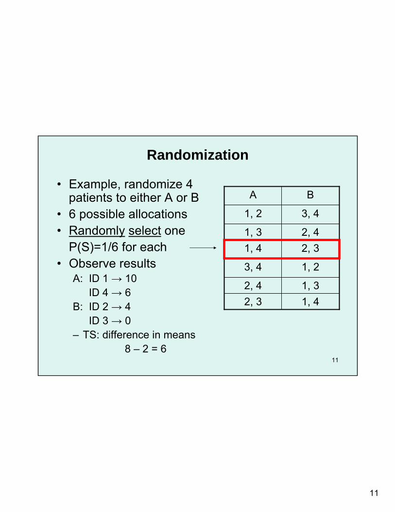
• Example, randomize 4 patients to either A or B

• 6 possible allocations• Randomly select one

P(S)=1/6 for each• Observe results

A: ID 1 → 10 ID 4 → 6

B: ID 2 → 4ID 3 → 0

– TS: difference in means8 – 2 = 6

1, 41, 3

1, 2

2, 32, 4

3, 4

B

2, 32, 4

3, 4

1, 41, 3

1, 2

A

12

12

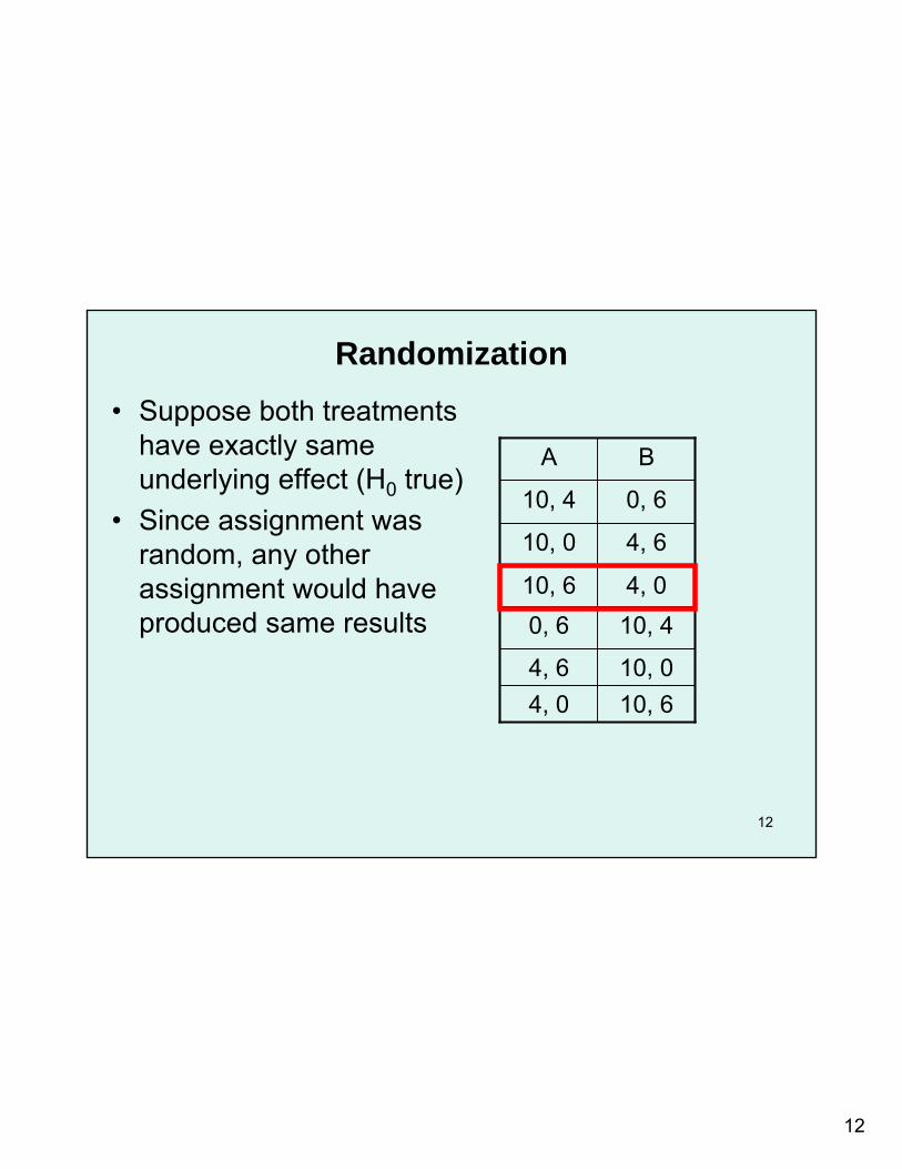
Randomization• Suppose both treatments

have exactly same underlying effect (H0 true)

• Since assignment was random, any other assignment would have produced same results

10, 610, 0

10, 44, 0

4, 6

0, 6

B

4, 04, 6

0, 610, 6

10, 0

10, 4

A

13

13

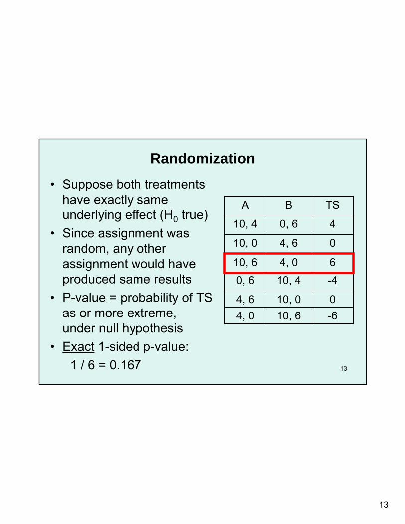
Randomization• Suppose both treatments

have exactly same underlying effect (H0 true)

• Since assignment was random, any other assignment would have produced same results

• P-value = probability of TS as or more extreme, under null hypothesis

• Exact 1-sided p-value:1 / 6 = 0.167

10, 610, 0

10, 44, 0

4, 6

0, 6

B

-60

-46

0

4

TS

4, 04, 6

0, 610, 6

10, 0

10, 4

A

14

14

Randomization

Q: What is the statistical inference space for results from a randomized experiment? – That is, to whom does this p-value directly apply?

a) Some larger population that contains “similar types” of people as those enrolled in the trial

b) The finite population consisting of all possible random assignments of the people actually enrolled in trial

c) Some other population altogether

15

15

Random Sampling from Infinite Population• Occasionally, study sample really is randomly

sampled from a huge or ambiguous population– E.g., randomly selecting clients from population of all

clients who attend a clinic in specific time period

16

16

Random Sampling from Infinite Population• However, more typically, random sampling is

implicitly assumed when– Applying statistical models, p-values, or confidence

intervals to observational data– Generalizing statistical inferences from an RCT to

some broader population• Such generalizations have been called non-

statistical inference, or inferences without a basis in probability

• “Clinical judgement” as opposed to “statistical inference”

17

17

“Arguments regarding the ‘representativeness’of a nonrandomly selected sample are

irrelevant to the question of its randomness: a random sample is random because of the sampling procedure used to select it, not

because of the composition of the sample.”

Edgington and Onghena (2007), Randomization Tests, 4th ed.

18

18

“I have never met random samples except when sampling has been under human control and choice as in random sampling from a finite population or in

experimental randomization in the comparative experiment.”

Kempthorne (1979), Sankhya

19

19

“In most epidemiologic studies, randomization and random sampling play little or no role in the assembly of study cohorts. I therefore conclude that probabilistic interpretation of

conventional statistics are rarely justified, and that such interpretations may encourage

misinterpretation of nonrandomized studies.”

Greenland (1990), Epidemiology

20

20

The Logic of Hypothesis Testing• Statistical hypothesis – a statement about

parameters of a population

• Null hypothesis (H0) – the hypothesis to be tested, often includes hypothesis of no difference– H0: Avg. BP in group A ≥ Avg. BP in group B

• Alternative hypothesis (HA) – corresponds to the research hypothesis– HA: Avg. BP in group A < Avg. BP in group B

• H0 and HA - mutually exclusive and exhaustive

21

21

The Logic of Hypothesis Testing• Goal of hypothesis testing – reject H0!• How do we decide to reject or not?

– Obtain data via a random process– If data are consistent with H0, then do not reject– Otherwise, if data are inconsistent, then reject H0 and

conclude HA

• P-value = probability of getting sample data as or more extreme than observed by chance, assuming H0

• Decision rule:– If p-value > α, do not reject H0

– If p-value < α, reject H0

22

22

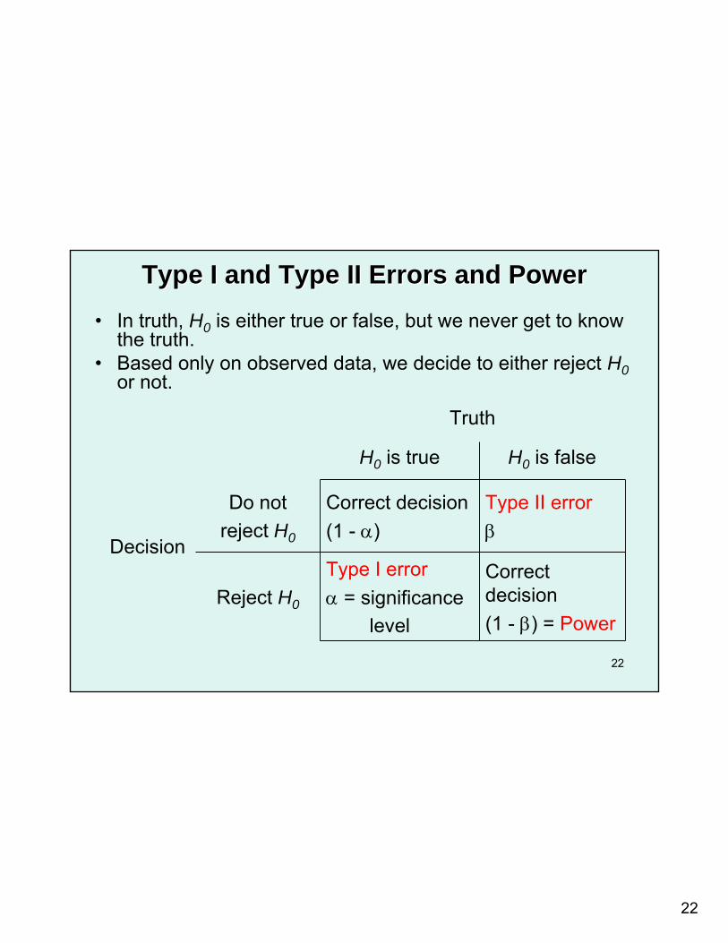
Type I and Type II Errors and PowerType I and Type II Errors and Power• In truth, H0 is either true or false, but we never get to know

the truth.• Based only on observed data, we decide to either reject H0

or not.

Truth

H0 is true H0 is false

Decision

Do not reject H0

Correct decision (1 - α)

Type II errorβ

Reject H0

Type I errorα = significance

level

Correct decision(1 - β) = Power

23

23

Interpreting Interpreting ““The Power to DetectThe Power to Detect””• Suppose protocol says “study has 90% power to

detect a mean difference between groups of 5.”

• This does not mean:1. There is a 90% chance to conclude that the true mean

difference between groups is at least 52. That there is a 90% chance of observing a mean

difference between groups of at least 5

• It simply means that there is an 90% chance of making a decision to reject the null hypothesis if the true (but unknown) mean difference is 5

24

24

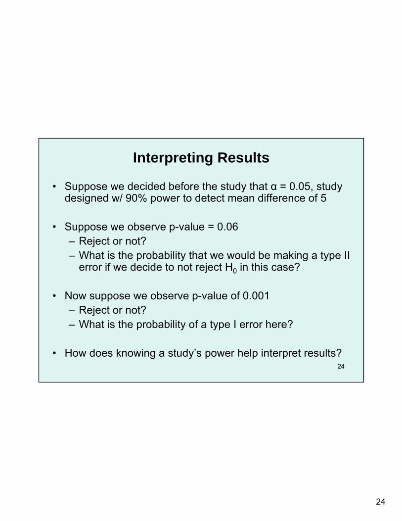
Interpreting Results

• Suppose we decided before the study that α = 0.05, study designed w/ 90% power to detect mean difference of 5

• Suppose we observe p-value = 0.06– Reject or not?– What is the probability that we would be making a type II

error if we decide to not reject H0 in this case?

• Now suppose we observe p-value of 0.001– Reject or not?– What is the probability of a type I error here?

• How does knowing a study’s power help interpret results?

25

25

Absence of Evidence …• Is not evidence of absence!• That is, not rejecting the null hypothesis does not

provide evidence that the null is true.• P-values provide evidence against the null.• Avoid the following conclusions:

– “no difference between groups”– “treatment was ineffective”– “no association between X and Y”

• Instead, say “insufficient evidence of” difference, effect, or association

26

26

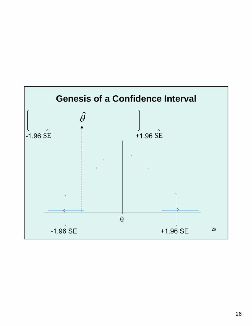
Genesis of a Confidence Interval

θ̂

SE∧

θ

-1.96 SE +1.96 SE

+1.96-1.96 SE∧

27

27

Interpreting a Confidence Interval

• For a 95% CI, we have 95% “confidence” that the true value is somewhere within the interval– This is not a probability statement– True value is either in the observed interval or it is not

• Have no more confidence regarding the center of the interval than we do around the endpoints– True value can be anywhere within the interval, not

necessarily near the middle– Point estimate should not necessarily be regarded as

“best estimate” or most likely value for true value

28

28

Confidence Intervals and Hypothesis Tests

• Close relationship between confidence intervals and hypothesis tests

• In fact, a confidence interval can be regarded as a family of hypothesis tests– Any value not contained within a (1 – α)% CI would

have been rejected by a 2-sided test of size α– Example: 95% CI for OR (1.25, 2)– CI does not contain the value 1– Thus, can reject H0: OR = 1 at the 5% level– CIs used frequently for conducting tests in certain

contexts, e.g., non-inferiority designs

29

29

Key Points

• Statistical inference requires a random process• Random sampling and randomization are not

the same thing• Goal of hypothesis testing is (almost) always to

reject the null hypothesis– Deciding not to reject tells you little– Don’t over-interpret non-significant results

• Confidence intervals provide a range of plausible values for true parameters, none of which is more “likely” to be the true one