Binomial data Bayesian vs. Frequentist conclusions...

Binomial dataBayesian vs. Frequentist conclusions

The prior

Binomial data

Patrick Breheny

January 15

Patrick Breheny BST 701: Bayesian Modeling in Biostatistics 1/29


The prior

The beta-binomial modelSummarizing the posterior

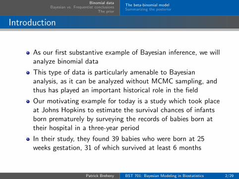
Introduction

As our first substantive example of Bayesian inference, we willanalyze binomial data

This type of data is particularly amenable to Bayesiananalysis, as it can be analyzed without MCMC sampling, andthus has played an important historical role in the field

Our motivating example for today is a study which took placeat Johns Hopkins to estimate the survival chances of infantsborn prematurely by surveying the records of babies born attheir hospital in a three-year period

In their study, they found 39 babies who were born at 25weeks gestation, 31 of which survived at least 6 months



The prior


Uniform prior

It seems reasonable to assume that the number of babies whosurvive (Y ) follows a binomial distribution:

p(y|θ) =

(n

y

)θy(1− θ)n−y

Suppose we let θ ∼ Unif(0, 1) (we will have a much morethorough discussion of priors later); then

p(θ|y) ∝ θy(1− θ)n−y

We can recognize this as a beta distribution; in particular,

θ|y ∼ Beta(y + 1, n− y + 1)



The prior


Conjugacy and the beta-binomial model

Suppose more generally that we had allowed θ to follow amore general beta distribution:

θ ∼ Beta(α, β)

(note that the uniform distribution is a special case of thebeta distribution, with α = β = 1)

In this case, θ still follows a beta distributon:

θ|y ∼ Beta(y + α, n− y + β)

This phenomenon is referred to as conjugacy: the posteriordistribution has the same parametric form as the priordistribution (in this case, the beta distribution is said to bethe conjugate prior for the binomial likelihood)



The prior


Summarizing the posterior

The fact that θ|y follows a well-known distribution allows us toobtain closed-form expressions for quantities of interest, forexample:

Posterior mean:

θ̄ = E(θ|y) =α+ y

α+ β + n

Posterior mode:

θ̂ =α+ y − 1

α+ β + n− 2

Posterior variance:

Var(θ|y) =(α+ y)(β + n− y)

(α+ β + n)2(α+ β + n+ 1)



The prior


Premature birth example

0.0 0.2 0.4 0.6 0.8 1.0

0

1

2

3

4

5

6

θ

Pos

terio

r de

nsity

θ̄ = 0.780

θ̂ = 0.795

SDpost = 0.064



The prior


Posterior intervals

Although the quantiles of a beta distribution do not have aclosed form, they are easily calculated by any statisticalsoftware program (e.g., the qbeta function in R)

Quantiles allow for the easy construction of intervals thathave a specified probability of containing the outcome

For example, we may construct a 90% posterior interval byfinding the 5th and 95th percentiles of the posteriordistribution

For the premature birth example, this interval is (0.668, 0.877)



The prior


Interpretation of posterior intervals

It is worth comparing the interpretation of this posteriorinterval (also referred to as a credible interval) with thefrequentist interpretation of a confidence interval

It is absolutely correct in Bayesian inference to say that “thereis a 90% chance that the true probability of survival isbetween 66.8% and 87.7%”

It is incorrect, however, to make a similar statement infrequentist statistics, where the properties of a confidenceinterval must be described in terms of the long-run frequencyof coverage for confidence intervals constructed by the samemethod



The prior


HPD intervals

Note that the quantile-based interval we calculated is notunique: there are many intervals that contain 90% of theposterior probability

An alternative approach to constructing the interval is to findthe region satisfying: (i) the region contains (1− α)% of theposterior probability and (ii) every point in the region hashigher posterior density than every point outside the region(note that this interval is unique)

This interval is known as the highest posterior density, orHPD inveral; in contrast, the previous interval is known as thecentral interval, as it contains by construction the middle(1− α)% of the posterior distribution



The prior


HPD vs. central intervals

For the premature birth example, the two approaches give:

Central : (66.8, 87.7)

HPD : (67.8, 88.5)

The primary argument for the HPD interval is that it isguaranteed to be the shortest possible (1− α)% posteriorinterval

The primary argument for the central interval is that it isinvariant to monotone transformations (it is also easier tocalculate)



The prior

Similarities to Frequentist approaches

In many ways, the conclusions we arrive at with the Bayesiananalysis are similar to those we would have obtained from afrequentist approach:

The MLE, θ̂ = 31/39 = 0.795, is exactly the same as theposterior mode and very close to the posterior mean (0.780)

The standard error,√θ̂(1− θ̂)/n = 0.065, is very close to the

posterior standard deviation (0.064)

The (Wald) confidence interval is (0.69, 0.90), close to theHPD interval (0.68, 0.89)



The prior

Proportions near 0 or 1

However, this is not always the case

For example, the Johns Hopkins researchers also found 29infants born at 22 weeks gestation, none of which survived

This sort of situation (and more generally, when the MLEoccurs at the boundary of the parameter space) causesproblems for frequentist approaches, but presents no problemfor the Bayesian analysis



The prior

Premature birth example, 22 weeks

0.0 0.2 0.4 0.6 0.8 1.0

0

5

10

15

20

25

30

θ

Pos

terio

r de

nsity

θ̄ = 0.032

θ̂ = 0

SDpost = 0.031

HDI95 : (0, 0.095)



The prior

Problems with frequentist approaches

In contrast, the (Wald) frequentist approach producesnonsensical estimates for the standard error (0) and a 95%confidence interval (0, 0)

To be fair, alternative frequentist approaches for constructingCIs exist for this problem, such as inverting the score test (0,0.117) and inverting the exact binomial test (0, 0.119)

However, these approaches do not always achieve correctcoverage – in this particular case, they both produce a moreconservative interval than the Bayesian approach



The prior

Informative vs. reference priorsJeffreys priorsPosterior as compromise

Informative vs. non-informative priors

Thus far, we’ve focused on the prior θ ∼ Unif(0, 1) as a wayof expressing a belief, before seeing any data, that allproportions are equally likely, or in other words a lack of anyparticular belief regarding θ

A basic division may be made between “non-informative”priors such as these and “informative” priors explicitlyintended to incorporate external information

These priors, and the resulting posteriors, serve differentpurposes: the former is in some sense an attempt to convinceeveryone, while the latter may be intended only to allow oneindividual reach a conclusion



The prior


Informative priors

Informative priors are well suited to research groups trying touse all of the information at their disposal to make thequickest possible progress

For example, in trying to plan future studies and experimentsabout possible drugs to follow up on, a drug company maywish to take as much information (from animal studies, pilotstudies, studies on related drugs, studies conducted by othergroups, etc.) as possible into account when constructing aprior



The prior


Reference priors

On the other hand, the drug company could not expect toconvince the at-large research community (or the FDA) withsuch a prior

Thus, even if the drug company did not actually believe in auniform prior, they might still wish to conduct an analysisusing this prior for the sake of arriving at more universallyacceptable conclusions

To emphasize this point, non-informative priors are oftencalled reference priors, as their intent is to provide a universalreference point regardless of actual prior belief (note: the term“reference prior” is given a much more specific meaning inBernardo (1979) and in later papers by Berger and Bernardo)

Other names include “default” priors, “vague” priors,“diffuse” priors, and “objective” priors



The prior


Problems with labels

The term “non-informative” is potentially somewhatmisleading, as all priors contain some information in somesense of the word

The term “objective” is potentially misleading when appliedto any analysis (frequentist or Bayesian), as fundamentallysubjective decisions must be made in terms of selecting themodel, distributional assumptions, etc.

A clear-cut distinction between informative and referencepriors is potentially misleading, as it is often reasonable to usereference priors for parameters of interest, and informativepriors for nuisance parameters



The prior


Information is not invariant

As an example of the problem in saying a prior has “noinformation”, consider transforming the variable of interest:

ψ = logθ

1− θOur uniform prior on θ, which stated that all probabilitieswere equally likely, is stating that log-odds values near 0 aremore likely than others:

−10 −5 0 5 10

0.00

0.05

0.10

0.15

0.20

0.25

Log odds

Prio

r de

nsity



The prior


Jeffreys priors

The statistician Harold Jeffreys developed a proposal for priordistributions which would make them invariant to suchtransformations, at least with respect to the Fisherinformation:

I(θ) = E

{(d

dθlog p(Y |θ)

)2}

Thus, by the chain rule, the information for ψ = f(θ) satisfies

I(θ) = I(ψ)

∣∣∣∣dψdθ∣∣∣∣2



The prior


Jeffreys priors (cont’d)

Now, if we select priors according to the rule p(θ) ∝ I(θ)1/2,we have invariance with respect to the information:

p(ψ) = p(θ)

∣∣∣∣ dθdψ∣∣∣∣

= I(θ)1/2∣∣∣∣ dθdψ

∣∣∣∣= I(ψ)1/2,

which is the same prior we would have if we parameterized themodel in terms of ψ directly

Various other formal rules for specifying automatic priordistributions have been proposed, although the Jeffreys (1946)approach is the most well-known



The prior


Jeffreys prior for premature birth example

For the binomial likelihood, the Jeffreys prior is θ ∼ Beta(12 ,12):

0.0 0.2 0.4 0.6 0.8 1.0

0.0

0.5

1.0

1.5

2.0

2.5

3.0

3.5

θ

Prio

r de

nsity

θ̄ = 0.788

θ̂ = 0.803

SDpost = 0.064

HDI90 : (0.686, 0.892)



The prior


Prior sensitivity

Note that the posterior didn’t change much between theuniform and Jeffreys priors

This is good; it would be an unattractive feature of Bayesianinference if two reasonable-sounding priors led to drasticallydifferent conclusions

This is not always the case – certain models or data can leadto unstable inference in which the prior has a large influenceon the posterior

This phenomenon is called sensitivity to the prior, and goodBayesian analyses often consist of several priors to illustratehow robust the conclusions are to the specification of the prior



The prior


Informative prior for premature birth data

Of course, an informative prior can exert greater influenceover the posterior

Let’s analyze our premature birth data one more time: thistime, let’s suppose that there had been some previous studiesthat had suggested that the probability of survival was around60%, and that it was rather unlikely to be close to 0% or100%

We might propose, in this situation, a θ ∼ Beta(7, 5) prior

Note that conjugacy is often helpful when thinking aboutpriors: this is the same as the posterior we would obtain witha uniform prior after seeing 6 successes and 4 failures, therebycarrying an “effective prior sample size” of 12 (or 10 morethan the reference prior)



The prior


Premature birth example, informative prior

0.0 0.2 0.4 0.6 0.8 1.0

0

1

2

3

4

5

6

θ

Den

sity

Prior Likelihood

Posterior

θ̄ = 0.745

θ̂ = 0.755

SDpost = 0.060

HDI90 : (0.647, 0.845)



The prior


Sequential updating

Note that the posterior we obtain, θ|y ∼ Beta(38, 13), is thesame as what we would obtain if we had started from auniform prior, stopped and conducted an analysis afterobserving 6 successes and 4 failures, then used the posteriorfrom that analysis as the prior for analyzing the rest of thedata

Indeed, we could have stopped and analyzed the data aftereach observation, with each posterior forming the prior for thenext analysis, and it would not affect our conclusions; this isknown as sequential updating



The prior


Posterior as compromise

Note also that the posterior is in some sense a compromisebetween the prior and the likelihood

This is true in a more formal sense as well:

α+ y

α+ β + n= w

α

α+ β+ (1− w)

y

n;

in other words, the posterior mean is a weighted average ofthe prior mean and the sample mean

This makes intuitive sense, as the posterior combinesinformation from both sources



The prior


Posterior variance inequality

Given that we are adding information from the data to theprior, one might expect that we have less uncertainty in theposterior than we had in the prior; this is also true, at least onaverage

Theorem: Var(θ) ≥ E(Var(θ|Y ))

Note that this is true generally for Bayesian inference; nothingspecific to the binomial distribution was used in the proof



The prior


Concentration of posterior mass

Indeed, letting θ0 denote the unobservable true value of θ,note that

θ̄P−→ θ0

Var(θ|y)P−→ 0

Thus, θ|y converges in distribution to one which places apoint mass of 1 on θ0

In other words, given enough data, the likelihood willoverwhelm the prior and there will no longer be anyuncertainty about θ (this is also usually true in Bayesianstatistics)


Binomial data Bayesian vs. Frequentist conclusions...

Documents

Transcript of Binomial data Bayesian vs. Frequentist conclusions...