t 'I i? ■‘ , *i THE UNIVERSITY OF TEXAS AT AUSTIN

V* l * ' ' " ' ' ! ‘ 1 '

i N

c * . ■ 1 . '' ■ ' ‘ '

' e ‘ /j # ' •

n 1 > ' ■ . ■ ■1 ■ " " (

t i -

e4V ■ .. ' • - '

X 4 i ■/ * . •

f •' , a. ■ . ,

o i ■ i ~ ■ ' nr

t .

/ • ' / ,/ *• • .

/ - . . • ■

p *

a - i < ' »

• / \ ‘ . • 11r

; • ‘ ' ■ j]C- ‘ • ■■ •; t : •

i * * .,c i

1 . ; ( , f »'e

; / ; * , *

T ■ x . - 1 „ ■ ’1 '

hG ’ f

' o . r ' » ■ . ■

y . ' ' ✓

</• " ■ ^

ORO 315

Solutions of Simple Dual Bootstrap Models Satisfying Lee-Veneziano Relation and the Smallness of Cut Discontinuities*

by

J*Charles B. Chiu, Monowar Hossain, and Don M. Tow

Center for Particle Theory, Department of Physics University of Texas

Austin, Texas 78712, U.S.A.

*Work supported in part by the 0. S. Energy Reserach Develop­ment Administration under Contract No. E(40-l)3992.

*Address for academic year 1977-1978: Laboratoire de Physique Th6orique des Particules Eltfmentaires, University Pierre et Marie Curie, 4 Place Jussieu, Paris, France.

1

Abstract

To investigate the t*dependent solutions of simple dual bootstiap models, we discuss two general formulations, one without and one with cut cancellation at the planar levol.We discuss the possible corresponding production mechanisms.In contrast to Bishari's formulation, both of our models re­cover the Lee-Venoziano relation, i.e., in the peak approxi­mation the Pomeron intercept is unity. The solutions based on an exponential form for the reduced triple-Reggeon vertex for both models are discussed in detail. We also calculate the cut discontinuities for both of our models and for Bishari's and show that at both the planar and cylinder levels they are small compared with the corresponding pole residues. Precocious asymptotic planarity is also found in our solutions.

-------------- notici-------- — —Thu rtport wh pnptrti 1 *» of wotk ipoM M d by UK Untud Sum Gm m iM M . N iIim i m UnJUd Sum not Ih l Uniud Stun D tpiitiw nl of Emtgy. not wtjr of dwli cmploym. tof iny of thflr cm uutott, wbeontrtcfort, of tlwli tmploywi, m U i any wi/rirtry, txpnu ot in p lk d ,« wumM uiy H |u UabUHy 01 mporafeiuty foi tht tourecy. tompUtttmi « uMhtam of iny tafsnwUon, «<wI<ki at pionM ddcloitd. tx (tptnm tt tfut IU u » mwM not Inftlm i prim tty o w .ii m hti._____________________

*

'•‘" M r 18 U N L I M I T E D ^

2

In the past few years, the strong interaction dynamical approach of "dual unitarization and topological expansion"1'2 has received considerable attention. This method may be con­sidered as the extension of the important work of Lee and Veneziano who using certain approximations derived the inter­esting result that the Pomeron intercept is a£ » l.3'5 In the approximation of neglecting momemtum transfer, t, depen­dence (called peak approximation in this paper), the Lee- Veneziano formulation turns out to be the first two terms, i.e., planar plus cylinder, in the topological expansion (TE).1 Higher order terms are supposed to be suppressed by powers of 1/N (SU(N) is the internal symmetry group), and some of these terms are further dynamically suppressed due to t-channel exoticity.

Since its introduction, much work has been done on thisapproach. For example( Chew and Rosenzweig6 showed that thePomeron-f identity is a simple realization of the TE, i.e., upto the cylinder level the Pomeron is just the f-trajectory,renormalized and mixed with the planar f'-trajectory via thecylinder correction to the planar approximation. This Pomeron-fidentity has already been shown to be a viable scheme phenomeno-

7-9logically. The effects of SU(N) symmetry breaking have been6 7 10-12 1 investigated. ’ ’ Inclusion of baryons and the next

14 15higher order term, the torus, ’ have been studied. The interesting property of asymptotic planarity was pointed out,®’*6

I. Introduction

3

2 (Okubo-Zweig rule for decays of mesons has been investigated.An important ingredient in the whole approach of dual

unitarization and topological expansion is the constraint ofplanar bootstrap, i.e., the input Regge poles should not befurther renormalized by planar loop insertions and therefore

2-5should be bootstrapped with the planar output Regge poles. ' Since the input kernel is a Reggeon-Peggeon cut, a natural question that arises is does the output at the planar level contain only poles, i.e., do the Reggeon-Reggeon cuts get cancelled in the solution of the integral equation. By choos­ing a specific form for the inhomogeneous term, it can be shown that such cut-cancellation does exist at the planar level.24 However, the generality of such a specific choice and therefore the generality of cut-cancellation has been

2 equestioned within the multi-Regge cluster framework. ’

By choosing an exponential form for the reduced triple-17Reggeon vertex, Bishari in an interesting paper was able

to investigate analytically t-dependent dual bootstrap equa­tions up to the cylinder level. His solution gives reason­able values for the Pomeron intercept and slope, and satisfies asymptotic planarity. He also found that even if a cut- cancellation mechanism exists at the planar level, the same mechanism does not lead to cut-cancellation at the cyliner level.

However, as will be shown in the next section, Bishari's

and elaborated on,17'19 and its relevance to the Itzuka-.21

22,23

formulation does not recover in the peak approximation tlio nice Lee-Veneziano relation of a® ■ 1. In this paper wo discuss two formulations of the dual bootstrap cqiuitions, one without and one with cut-cancellation at the planar level.We discuss the possible production mechanisms which load to these two formulations. Both formulations, in contrast to Bishari's, recover in the peak approximation the lee-Vencziano

relation. Following Bishari's approach in solving this type of equations by choosing an exponential form for the reduced triple-Reggeon vertex, we solve tnese equations for the Pomeron intercept and slope. We then calculate the discon­tinuities of the Reggeon-Reggeon cuts at the cylinder level for both formulations and found that they are small compared with the corresponding pole residues. In the formulation where a Reggeon-Reggeon cut does exist at the planar level, this cut discontinuity also is calculated and shown to be small compared with the planar pole residue. Finally, weprovide further support for precocious asymptotic planarity,*6 ’*7,19

2i.e., the cylinder contribution is already small at t i 2 GeV .The theoretical formulation of the bootstrap equations,

together with their solutions in integral form, is prerented in Section II. In Section III, based on an exponential param­eterization for the reduced triple-Reggeon vertex, we inves­tigate the solutions, the cut discontinuities, and asymptotic planarity. Section IV ends with a short summary. Derivations of certain equations are contained in Appendix A. Modification duo to the no-double-counting condition is discussed in Appendix B.

4 5

II. Bootstrap Equations and Their Solutions in Integral FormA. Bootstrap Equations

The dual bootstrap equations have been discussed by many authors. However, the specific forms differ in details among authors. Here we briefly discuss our two formulations to establish our conventions, and explicitly state the assump­tions involved.

First wc look at the planar bootstrap equation. This is depicted in Fig. la. In terms of the energy variable, it reads (we leave out writing explicitly the dependence on the overall t),

Alb(s) ’ AlbCs) + Tlb(s) * (2,1) ith s slb(s) - dslA°2( s ds2A2bCs2)fd*2(If ^ ) a2+a2' z2 . (2.1a)

o

where “ cosn^-o^i) and in general = a(t^), ou , = a(t|). In (2.1a) we choose to expand the asymptotic behavior of the Reggeon loop in powers of (s/sjs2), where sj » Sj-sc . This shift from the more commonly used Sj variable to the present sj variable is a simple way to get an exact factorizable kernel and at the same time satisfy the constraint of the finite range interaction, and also (as we shall see later) to realize duality and cut cancellation associated with model II. Duality in the present context states that the appropriately weighted cluster production contribution can be evaluated through finite mass

6

sum rule (FMSR). The A(s)'s are the absorptive part of the various amplitudes. Subscripts i remind us that the relevant Reggeons are at and ,, and the corresponding quantities in general have tj and tj dependence. The phase space volume element, which depends on t2 and t£ is denoted by d$2* See Eq. (A-l) of Appendix A for details.

Performing the Mellin transform, we get the "effective- partial wave amplitude,"

Aib (J) S f dsAlb(s)s'J'1 - A°b(J) + Tlb(J) , (2

" d So

A ^ U ) 5 J dsA^CsJs’11-1 ,

nd . s0lb(J)- f d*Tlb(«)s'J‘l

•'sC y /•” r ” a 2+a2 ,-J.

&$2zz j dslA12(sl)sl J J ds2A2b^s2^2 J s[s'2 (s|s2)

“ f d*2B12z2 ’ (2-3)

where

aci 5 °i + ai' ‘ 1 ’ (2.3a)

B j 2 = J d s ^ f s p s ' ^ Z ^ Z ' . (Z#3b)

'so

Notice B°2 is not the-Mellin transform of A12(Sj) (see also Appendix B).

Up to now, the formuletion is general. The different formulations mentioned at the beginning of this section correspond to different choices for the Reggeon-particle in- homogeneous term, i.e., for A°b(s) or equivalently for Ajb(J). We discuss two choices. They correspond to two different production mechanisms for the end particles of the multi­peripheral chain.

In model I, we assume that resonances or clusters are also produced at the two ends of the multiperipheral chain and that their average spectrum is, as that produced in the interior vertices along the multiperipheral chain, approxi­mately given by the extrapolation of the leading Regge pole behavior down to the low energy region. Taking into accountthe most pronounced t^ and tj dependence, which is due to the

FIfirst nonsense-zero factor, we parameterize the inhomogeneous term as

Alb(s) - d1(a-acl)(s-so)a0(5--s)eCs-so) , (2.4)

where a = aft) and dj ■ d(t,t1,tp, which is presumably a smooth function of t, tj and t{ in the kinematic region of interest. In turn,

A°b(J) = fjgjYj , (2.4a)with >s-

1 d A M

8 9

We note that gj is a triple-Reggeon vertex.

Carrying out the integral explicitly, we get

'“ -J iQ+1

F2

" «Vr (r- - 0 F U lf«*is«*2;-(i - 1) • (2.4c)

In the limit of large s/sQ,F3

a-J/s T 1 /s V J ‘ X . r (a + l)r (J -a ) / s Y 01' 1! o f o - 1) + k nbir \t;) J-

(2.4d)

One can explicitly check that as expected there is no pole at J ■ a. For our discussion below, it suffices to know that Yj does not contain any tj, t£ dependence and it is a smooth function In t at least for a > -1.

In model II, we assume the two end particles in the multi­peripheral chain maintain the identity of the two incident particles (this we shall Tefer to as "the leading-particle-dominance ansatz") F4 More specifically denoting the leading

particle mass-square by m , we have

Since 3" is the direct-channel-ground-state pole residue, it is plausible that it should be a smooth function of tj and t^. Furthermore, in order for the Reggeon-Reggeon cut to cancel at the planar level, one has to assume that d^ and cTj have the same dependences on t^ and t^, such that their ratio is independent of tj and tj. This will be assumed for model II for the rest of the discussion in this paper. Thus, for model II,

1 * gl " ‘,i<«-acl) ’ and YJ “ * (Z-Sc)* “ “cl

where ¥ "lay depend on t. The inhomogeneous terms for models I and II are illustrated in Fig. lb.

For both models the Reggeon-Reggeon amplitude in the kernel is assumed to take the same form. In particular, from (2.4) and (2.4b) and factorization, it is given by,

A j2 (s l) * g1 (s1 -s0)a g2e(s-s1)e(s1 -s0 ) . (2-6J

A ° b (s) * ^ ( s - m 2 ) ,

and

A l b (J ) = figjYj ■

Here as before, gj ■ ^(a-o^), but

(2.5)

(2.5a)

(2.5b)

So

o r S a ’a 2'a 2<B 12 ■ ®1®2J d s l (sr V >

a 'a r2(s-s0 ) CZ

®1*2 a-ot.*c2

■ °2 S 8lh2 •

(2.6a)

(2.6b)

10

where hj is a smooth function of tg and t^.The result (2.6a) is just the expected FMSR result,

consistent with the duality assumption stated earlier. Wealso mention that the — ~— factor in the same expression ® "°c2will be playing a crucial role in achieving the cut cancella­tion. This factor can be traced to be due to the coincidence of the branch point associated with the assumed Regge power

behavior in A®2 (s.), and the branch point of the weight factor (s|) 4 L . Such coincidence is expected if we asso­ciate the branch points in question with the lowest physical threshold. Within our parameterization this assumption is implicitly incorporated through the introduction of the s£ variable in (2.1a).

To simplify the notation, we denote the partial wave amplitude at the planar level by

R i s A i b W ■

Our integral equation at the planar level now takes the general form

R1 ■ W j ♦ h j d*2

with f^ * 1 for model I and f^ ■ (“ -“(-i)'1 f°r model II.For model I, since Regge behavior is assumed for both

and A°2 . they have common tj and tj dependences as the

11

result of the factorization property. On the other hand, for model II, factorization is not expected in view of the leading-particle-dominance ansatz. Model II gives essen­tially the cut-cancellation type of models originally pro-

2 Aposed by Bishari and Veneziano, and subsequently further considered by various authors.24-26 these authors ob­

served, such type of models leads to cut cancellations.The bootstrap equation up to the cylinder level is de­

picted in Fig. lc. Denote the partial wave amplitude for the Reggeon-particle scattering up to this level by Pj (where the Reggeons are and a^,). Analogous to (2.7), for the present

case,

r h,(z2+l)P,P1 ■ fl*lYj + *ljd*2 -V „c-2 - * <2'8)

B. Solutions to the Bootstrap Equations Denote

i (A)“ l d*i * (2,9)

and

where Zj(A) - cos[An(a1-a1,)], and X » 1 and 0 corresponding to the uncrossed and crossed Reggeon loop respectively. Note

12

that 2^(1) ■ Zj and z^(0) »'l. Also note that both Fj(X) and Gj(X) have cuts in the J-plane.

From (2.7) we get,

8tY,G.(l)

Ri • {i H ' j * 1 - PJ H T • ( 2 . H )

The planar Regge pole occurs at J » a, or

^ ■ f i r ^ ’ 1 • (2-12>

Equations (2.12) and (2.9) together with (2.7) give

gtYjGjCl)R 1 “ f l®l^J * H j d J T l - T T * (2-13)

whereF (A) - F . U ) f g n h j Z ^ X )

hj M - - J d*i . C2-14)

This is the general expression for R^, applicable to both models I and II. In the case of model II, (2.13) simplifies. From (2.5b), Gj(l) » Hj(l). In turn we get the cut cancella­

tion result:24’2®

g . y j U - a . , )

Ri ‘ • <2-15>

Foi the Pomeron, making use of the analogous steps lead­

ing to (2.11), we have

13

glYj[G,(l) ♦ G.(0)]pi " figiYj * i - FjOj- -~Fjarr • (2-16)

The Pomeron pole occurs at J » op = <*p (t), or

F (1) + F (0) - fd*. (z,+l) « 1 . (2.17)P °P J 1 aP acl i

Results (2.16) and (2.17) are applicable for both models I and II, where the only difference between the two models is in the forms of Gj and Yj*

It is instructive to recast (i.16) in a different form. We write,

gjYJG.d) + G .(0) ]P1 * flBlYJ + (J-a)Hj(l) -■ FjUJ)- ’ V ' 16*)

orr

+ z j r r p W j * v t t x

1J"1

+ •r gt(o)i ....................................

{lslyJ * Yjj_X + SJZTTJ (R1 + R1C2JR2 + R1C2JR2C3JR3 (2

where

R1 ' £lglYJ _ glGJ ^ _ FJ ^ rt -----^ ------(J-ot)Hj(T) and C1J gjGjdJ • C2

••)

.16b)

.16c)

14

Equation (2.16b) indicates that we can also regard the Pomeron as the iteration of a suitably defined Reggeon term R^ to­

gether with a suitably normalized cylinder kernel Cj.We now verify explicitly that both models recover in

the peak approximation the Lee-Veneziano relation of a£ » 1. Notice that (2.12) is applicable to both models. At t • 0,

*1 " tl- “ 1 ^or both X ■ 1 and X « 0. From (2.12),in the peak approximation we have

* (2’18)J cl a0-a.

with otQ = a(0) and a® = 2aQ - 1. So

1 - a0 . (2.19)

On the other hand, the Poaeron intercept is given by the zero of the denominator of the Poineron equation (2.16a), which is again applicable for both models. It leads to

6lhl

«lhl 1

J - a - ---^--------Si------ , (2.20)

which in the peak approximation reduces toc

J ' ’ -- -J- c-C--- - “o - °c ' (2'21)(J-a°)(a0-a°)

IS

giving the desired result

aP “ 2«0 - " 1 • (2,22)

17Wo now compare our model II with that of Bishari.His planar bootstrap constraint, after taking into account the relation gjhj - g2(Bishari)/(a-acl), is identical to our Eq. (2.12) (or (2.18) in the peak approximation). Irom his Pomeron equation, his Pomeron intercept is given by

f glh i ( « - « c l )- a J - i,c~ » (2>23)

which in the peak approximation becomes

c(o -o°)J - “o - . o ■ (2-Z4^

J ' “c

(J-ac)(J-a°) - (l-a0)c . (2.25)

Making use of (2.18), we find the solution to be

„ 3a -1 + /5'(l-o„) a° - ---- 2------ — , (2.26)

which gives a£ s 0.81, if a nominal value of a0 » 1/2 is used.For the Pomeron equation, if we compare ours, Eq. (2.21),

with Bishari's, Eq. (2.24), we get

16

J-a° c(a -a°) J-a°<J'“o W ------r ^ < J -“o^Bishari ' <2-27’

J'“c

We see that the difference is a factor (J-a°)/c, which from (2.18) is unity only for J » aQ . In general, and in particu­lar for J « otp, this factor is not unity.

17

III. Simple Solutions, Cut Discontinuities and Asymptotic Planarity

We divide this section into three parts. In part A we discuss the Pomeron intercept and its slope, in part B we estimate the cut contribution to the amplitude at both the planar level and cylinder level, and in part C we discuss quantitatively the approach to asymptotic planarity in our models.

A. Pomeron Intercept and Its SlopeWe recall from (2.4b) and (2.6a) the quantity

gjhj - d2(a-acl)(s-s0)“ °cl , (3.1a)

where as stated after (2.4) d^ is presumably a smooth functionof t, t,, tj. Since (s-s )a'acl is also a smooth function of

° 2 — “'“clt, t^, tj. We parameterize the product dj(s-sQ) by anexponential and write,

g ^ - k2Ca-acl)eat+bCtl+tl) . (3.1b)

Here, k, a and b are constants, and the Regge trajectory isa = a + a't. This form was first considered by Bishari1^oin connection with dual bootstrap equations.

For later comparison with the triple-Reggeon vertex ®RRR t*lat various people have extracted from phenomenological analysis, we note that

< 4 r * 4 - glhx(a-acl)(s-so)'(a'acl) . (3.10

18

T h u s « ^ - “ c l 3 h2 ~T~*gl • k(a-acl)(s-s0) 2 e 2 2 1 1 . (3.Id)

g*The smooth function — is what we called the "reduced

“‘“cltriple-Reggeon vertex."

The planar bootstrap equation (2.12) gives (see Eq. (A-5) in Appendix A) Bishari's conditions,

“ 1 C3,2a)

i _2 ,2 a = - £(b + 2-g— ) . (3.2b)

The conditions for output Pomeron pole, (2.17), gives (see Sq. (A-10) in Appendix A),

1 “ jp-l<V 0,lexP

ir2o ,2tX + e (3.3)

where ac s a° + , with a° » 2a0 - l as defined earlier.Equation (3.3) is exact. Later in the discussion on

asymptotic planarity, we will solve it by a numerical method. For now, we concentrate on the region of small t and solve the linearized version of (3.3).

For small t, (3.3) can be written as (see (A-15) in

Appendix A)

19

(3.4)

Now assuming that in this region the Pomeron trajectory is linear in t, ap s a° * a£t, we can expand the right hand side of (3.4) in powers of t, and set the coefficient of each power to zero. This gives, up to first order in t, the following two equations (see Appendix A for details).

£ ( “ p - a o ) e ^ P ° E l £ “ 1(3.Sa)

and

~alpSqr ~ 1 b /“P . l\ V

o _ aT \ a7" 2/

b - “ P 1 ,- f b - \ ?tPo EF - I , it2 _

0/ ---- 5 ---- * I B Mpo

(3.Sb)

where pQ = <*£ - a®, and E^(x) is the exponential integral 28function. This linearized approximation will later be

2shown to be well justified for |t| < 0.5 GeV .

2ftFor large z,

(3.6)

If we evaluate (3.Sa) in the peak approximation, i.e., let b •* ", then (3.5a) becomes

20

Z«*p-<V - P0 - «p - 2“0 ♦ 1(3.7)

recovering the expected Lee-Veneziano relation.We take aQ to be its nominal value of 0.5. Then for

each value of b/a', (3.5a) gives a solution for a^. i'hen from (3.5b) one can solve for <*p/a'. In Fig. 2a we plot <x° and a^/o' versus b/a'. To make a direct comparison between a£ and a£, we plot Fig. 2b. Some discrete values of b/a' are

also shown along the curve. For example, we find that for increasing from 1.10 to 1.3S, a£/a' decreases from 1.20

to 0.02.If we choose a nominal value of 0.5 for Qp/a' and a' «

1 GeV”^, our solution gives a° = 1.27 (corresponding, to b =_ 7

3.2 GeV ). In this simple model, the Pomeron intercept turns out to be a little high. However, we emphasize that our numerical result follows from the particular parameteriza­tion (see (3.1b) and (3.1c)) of gj, the triple-Reggeon vertex, which was chosen so that we can do the integrals analytically. Hopefully, with a more realistic choice for gj, a more realistic emerges. The results of Ref. 19 suggest that this may indeed be the case. This problem deserves further in­

vestigation.In Fig. 5 we plot the tj-dependence of g1(0,t1,t1) at

21

t = 0. We choose b = 3.2 GeV as discussed in the previous para­

graph. For s, the cluster mass cutoff, we consider two— — 2 cases. Case a: ln(s-sQ) = 1 (or s s 3 GeV ); case b:

__ — 2ln(s-sQ) s 2 (or s s 6 GeV ). These two curves are plottedin Fig. 3 along with several other parameterizations dis­cussed in the literature.2,2®'3® The parameterizations of Refs. 2, 29, and 30 are respectively, (1-1.Stj)*!, e*3tj^ and 0.8e*®,: + 0.2e^*l. In these three references their parameterizations are actually for the product of gj and two external particle-particle-Reggeon vertices. Due to the non-leading nature of the triple-Reggeon contribution, there is large uncertainty in estimating its t^ dependence. Notice that Ref. 2 ’s parameterization is very much different from those of Refs. 29 and 30; this may be partly due to the dif­ferences coming from different energy ranges aiid different reactions considered. Our value of b/a’ is well within the range of values these authors have considered.

B. Cut DiscontinuitiesWe now proceed to look at the J-dependence of the ampli­

tudes away from the pole, in particular, in the Reggeon-Reggeon cut region. We shall calculate the discontinuities of these cuts. In this part we shall restrict ourselves to t = 0, thus Z l (l) = z ^ O ) - 1.

We first start with model I. In this case from (2.9) and (2.10)

_ 2

Gj(X) = Fj(X) , (3.8)

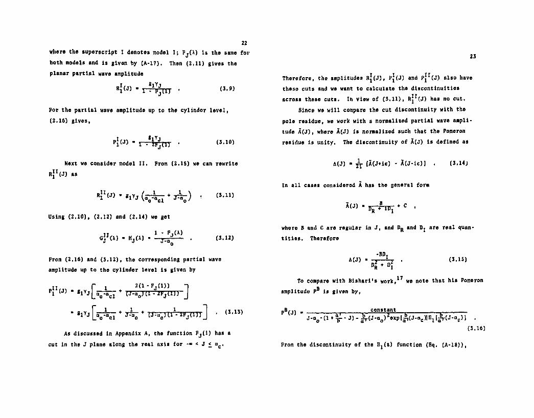
where the superscript I denotes model I; Fj(X) is the same fov both models and is given by (A-17), Then (2,11) gives the planar partial wave amplitude

»}(« - • (3,9}

For the partial wave amplitude up to the cylindor level,(2.16) gives,

p i (J) “ r ~ ^ Pj ii y • (3,10)

Next we consider model II. From (2.15) we can rewrite r J^J) as

Rr < J> ' *1>J + 3 ^ ) <

Using (2.10), (2,12) and (2.14) we get

Gj M ‘ HjCAJ - - j - i --- . (3.12)

From (2.16) and (3.12), the corresponding partial wave amplitude up to the cylinder level is given by

r n m - n ir T 1 ■ 2 ( 1 - FJ (1)) 1P1 (J) ‘l ^ V ^ l " W'*o™ - ZFjTlTT J

" BlYj [v^T+ ^ +

As discussed in Appendix A, the function Fj(l) has a cut in the J plane along the real axis for -• < J < “c*

22

23

Therefore, the amplitudes R*(J), pJ(J) and pJ*(J) also have these cuts and we want to calculate the discontinuities across these cuts. In view of (3.11), r |1(J) has no cut,

Since we will compare the cut discontinuity with the pole residue, we work with a normalized partial wave ampli­tude A(J), where A(J) is normalized such that the Pomeron residue is unity, The discontinuity of A(J) is defined as

A(J) - ti- [A(J+ie) - X(J-ie)] . (3,14j

In all cases considered A has the general form

* (J) " D j p iDJ * C •

where B and C are regular in J, and Dg and Dj are real quan­tities. Therefore

-BD.A(j) . — L_ . (3,15)

To compare with Bishari's work,17 we note that his PomeronDamplitude P" is given by,

pBjjj m ________________ constant _______J- V (1 ♦ t t * J) ' |r(J-‘»o)Zexpl^(‘,-ac)>EllfrCJ-<»c)] .

(3.16)

From the discontinuity of the B^(z) function (Bq, (A-18)},

24

tho discontinuities in our models as well as in Bisheri's model can then l>e easily calculated.

We plot in Fig. 4 tho discontinuities for r |, pj, pj1 and P® as a function of J from the branch point J ■ 0 down to -1.

Near the branch point J ■ a® ■ 0, A® is the largest, and Ap and Ap1 are comparable. For the latter two, from (3.10) and (3.13) and the normalization convention for A, there is the relation

The corresponding power behavior in the full amplitude associated with the discontinuity in the partial wave ampli* tude at J is sJ (when applied to an internal link in a multi* peripheral chain, s should be replaced by the subenergy Sj i+1)- Because the tip of thn cut lies approximately one-half and one unit below the Reggeon and Pomeron poles, respectively, the cut contribution is already much suppressed by this energy factor.

Now we want to show that even without taking into account this energy factor, the area under the cut discontinuity function shown is already significantly less than the pole contribution in the same partial wave amplitude. More pre­cisely, we consider the ratio

25

where for definiteness we take Ic ■ / £ -dJA(J)» and it iscto be compared with the pole contribution in the same am­

plitude given by itr, with r being tho pole residue. For the

Pomeron amplitude, by construction the residue of the pole is r ■ 1. For the Reggeon in R1, its pole residue is r >0.48. We then find n • 0.08, 0.03, 0.02 and 0.04 for R1, P1,P11 and PB , respectively. Thus the contribution of the cut is indeed very negligible both at the planar and at the

cylinder levels.

C. Asymptotic PlanarityHere we investigate the Bsymptotic planarity in our

model. Equation (J.3) can bo rewritten as

1 “ j r X e x p f j r (X ♦ 1 - a0 ♦2 2

* f ’ $ - 4 ¥>¥■ * • ] ■L J (3.17)

where X = ap - a.It is instructive to compare the planar and the cylinder

contributions in the integrand. Note that the planaT con-_2 , 2 t

trlbution has an extra factor of e x p — )• which stems from the planar Reggeon phase factors. This extra factor grows exponentially with t, in the positive t region, resulting in the dominance of the planar term, or asymptotic planarity.On the other hand, in the negative t region, the same factor

26

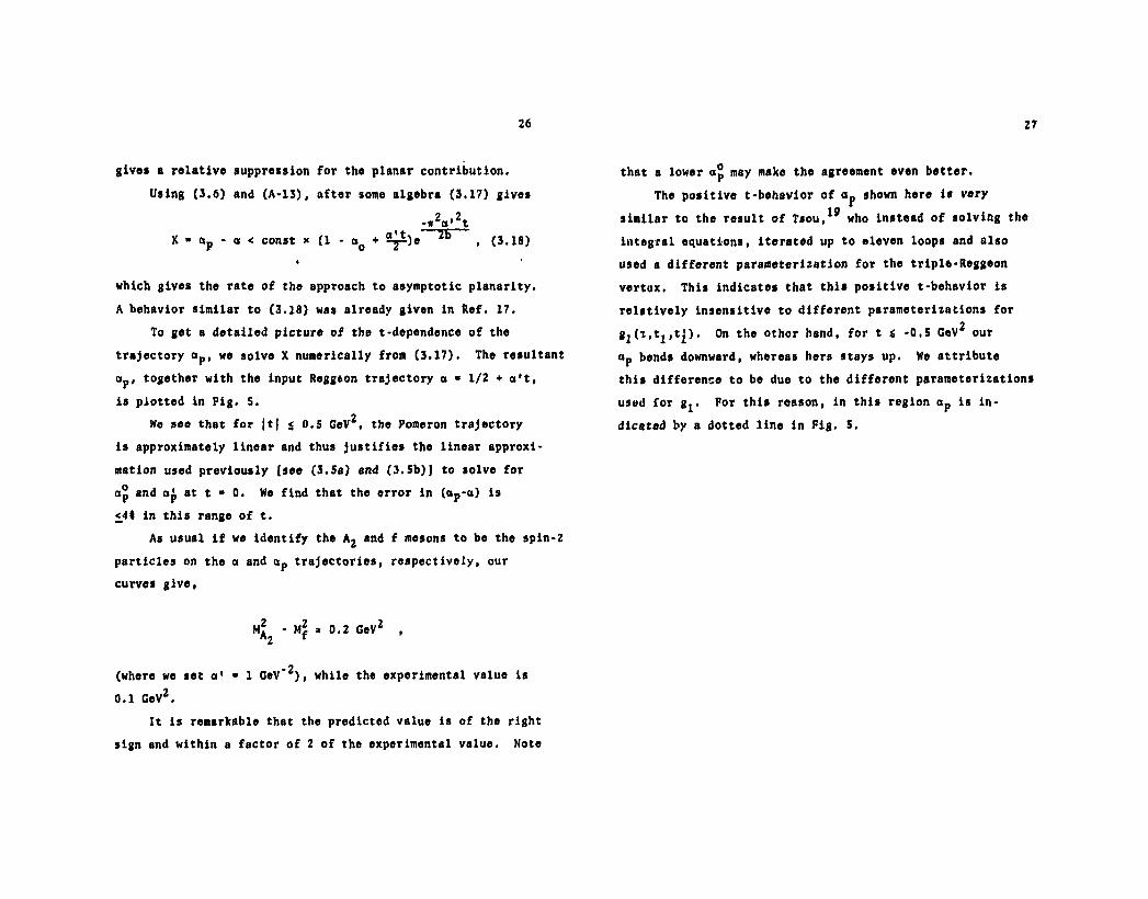
gives a relative suppression for the planar contribution.Using (3.6) and (A-13), after some algebra (3.17) gives

-11 o 12tX ■ (*p - a < const x (1 - c»0 ♦ ^-)e ^ , (3.18)

which gives the rate of the approach to asymptotic planarity.A behavior similar to (3.18) was already given in Ref. 17.

To get a detailed picture of the t-dependence of the trajectory ap, we solve X numerically from (3.17). The resultant ctp, together with the input Reggeon trajectory a ■ 1/2 + a't, is plotted in Pig. S.

We see that for |t| < 0.5 GeV , the Pomeron trajectory is approximately linear and thus justifies the linear approxi­mation used previously [see (3.5a) and (3.5b)} to solve for

and a£ at t • 0. We find that the error in (ap-a) is <41 in this range of t.

As usual if we Identify the A2 and f mesons to be the spin-2 particles on the a and ap trajectories, respectively, our curves give,

ma 2 ‘ Mf * 0,2 GevZ *

(where we set a' ■ 1 GeV*2), while the experimental value is 0.1 GeV2.

It is remarkable that the predicted value is of the right sign and within a factor of 2 of the experimental value. Note

27

that a lower otp may make the agreement even better.The positive t-behavior of Op shown here is very

similar to the result of Tsou,*^ who instead of solving the integral equations, iterated up to eleven loops and also used a different parameterization for the triple-Reggeon vertex. This indicates that this positive t-behavior is relatively Insensitive to different parameterizations for gj(t.tj,tj). On the othor hand, for t s -0.5 GeV2 our Op bends downward, whereas hers stays up. We attribute this difference to be due to the different parameterizations used for g^. For this reason, in this region ap is in­dicated by a dotted line in Fig. 5.

28

IV. SummaryWe have presented two formulations of the dual bootstrap

equations: one without and one with cut-cancellation at the planar level. Both formulations in the peak approximation recover the Lee-Veneziano relation of - 1. Choosing an ex­ponential form for the reduced triple-Reggeon vertex, we solved these equations. We showed how the discontinuities of the Reggeon-Reggeon cuts can be calculated. We found that at the cylinder level, the cut discontinuity in both models (and also in Bishari's) is small compared with the Pomeron pole residue. Even though in model I the Reggeon-Reggeon cut . not can­celled at the planar level, we found that its, discontinuity is small compared with the planar pole residue. This important result indicates that the planar pole bootstrap constraint can be satisfied to a good approximation even if there is no cut- cancellation mechanism. We provided further quantitative support for precocious asymptotic planarity in the positive t region; we also found that in the large negative t region, ap depends more sensitively on the parameterization of the triple-Reggeon vertex.

29

Appendix A: The Fj(*) Functions, Reggeon and Pomeron Con­straint Conditions

We recall that the Fj(*) functions are defined as

■/» ii 8 1 ^ 1 )

■ h i - J-Vi - - - C2.9)

where X « 1 or 0, Zj^l) = cosn(a-ap, and Zj(0) » 1. In this Appendix we give the derivations of Fj(l) and Fj(0) for the parameterization considered in Sec. Ill,

2 at. + b(t.+t,')glhz - k*(a-acl)e 1 1 . (3.1b)

For completeness, we will also include tho details leading

to the Reggeon condition (3.2) and the J’omeron equations(3.3) and (3.5).

The two-body phase space volume element is given by

d*. = -5L.dt.dt' SIS! . (A-l)1 16n 1 1 /K

In high energy small angle approximation,31

| | (2i+l)P|l(cos9)P)l(cose1)P4(cos8')/X

= j f dbbJD (bw)J0(bu)J0(bv) , (A-2)**0

where u2 ■ -tj, v2 ■ -tj and w2 ■ -t. The factor N is

30

associated with the SU(N) symmetry assumed. For a planar loop, N is the number of windows. On tho other hand, for the cylinder loops, N is present only when the crossed channel is an SU(N) singlet. This is the case in the present work.

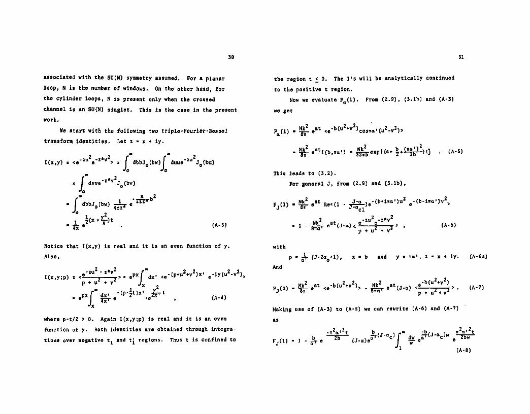
We start with the following two triple-Fourier-Bessel transform identities. Let i • x + iy.

2 2 C 2I(x,y) = <e'zu e'z*v > = | dbbJft(bw) j duue‘*u J0(bu)J dbbJ0(bw)j o J o

r /: ,

- ^ eZ x . (A-3)

x | dvve"z*v J0(bv)

x 2- | dbbJ0(bw) ^ e'7^

Notice that I(x,y) is real and it is an even function of y.Also,

I ( x ,y ! p ) B ■ e P ^ f d x ' < e*^P+ u 2 + v 2 ^x ' , - i y ( « 2 -v2 )>P + uz + vz Jx z

. eP * f ’ | ; e - tP^ X,, ^ t , (A-4)■'x

where p-t/2 > 0. Again l(x,y;p) is real and it is an even function of y. Both identities are obtained through integra­tions over negative t and t£ regions. Thus t is confined to

31

the region t < 0. The I's will be analytically continued to the positive t region.

Now we evaluate F0(l). From (2.9), (3.1b) and (A*3)we get

p (i) m Njd eat <e"b u2+v ^cosna'(u2-v2)>O ' Off

■ IT*- eatI(b,ira') * J77I? exPl (a+ 7 +^2b^ * A’5^

This leads to (3.2).For general J, from (2.9) and (3.1b),

Fj(1, - ?*!e8t Re<(l - Jia_)e*(b+il"l')u2

MV2 a* »*Zu2«'Z*v2■ 1 - jfljfr e («*■«) < ---- 2----1 * * (A-6)B1,a p + u + v

withp ■ jjr (J-2ao*l), x ■ b and y • iro', z ■ x + iy. (fi

And

Fjtw ■ % - •“ <‘M “ *’ ’> • f e •“ « - ) •

Making use of (A-3) to (A-S) we can rewrite (A-6) and (A-7)

(A

as

F j U ) . i . .b. e ~ l r (J-a)e f — eo^^"°c)w

1 (A-8)

-6a)

-7)

From (A-8), (A-9) and (2.17), the Pomeron condition gives

1 . . T S 1 ] .

which is Bq. (3.3).To proceed further, we make use of the exponential

28integral function defined by,

.-*t

(A-10)

»„<’> ■ / - , n - 0,1,2,... (A-ll)

which satisfy the recursion relation

(A-12)

We can now rewrite (A-9) as

- * v 2 tFj(0) • e ~ZF

For small t, the last factor e and (A-8) becomes

f l - ( J - a J e ^ ' ^ E J l r (J-<*c) ] .

^ n2a'2t J (A --------zBw- (^.8) Can be expanded

13)

33

-if o' t r ■> b ,, „ i■25— ,T J it a't b~ T

[i - ^ ( j . ^ J e ^ J - ^ ) ]

(A-14)

In this small t approximation, the Pomeron condition 1 -

Fap(l) ♦ Fop(0) becomes

l ■ (a a1 f 4 ^b 3 T (aP °c ^ - [” b , il1 - (ap-a) j — j — ♦ j r e Ex (<*p-ac)J

x £ . (ap-ac)J j ♦ 0(t2) , (A-1S)

which is Eq. (3.4). Setting ap : aj| + a£t and expanding theright hand side of (A-1S) in powers of t, and using E.(z + Az) =

-2Ej(s) Az, we get

♦ 0(t2) , (A-16)

where P0 = °p • This gives the Pomeron conditions (3.Sa) and (3.5b) of text.

From (A-13) and (A-14) note that at t * 0, we get

Fj(l) • Fj(0) - 1 - (J-“0)e“T(J C‘c)B1 • (A-17)

34

The function Ej(z) has a cut in the z-plane along the nega­tive real axis. Setting z ■ u + iv, the cut is from u ■ -» to 0. The complex value of Ej(z) just above and below the cut is given by

Ej(-u + ie) ■ -Ei(u) + iir , u > 0 (Awhere _

f -tEi(u) ■ -P J S— dt , u > 0 J-u

■ Yo + lnu + J.HTTi • fAn»i

with the Euler constant ■ 0.577. From, (A-13) and (A-14) we see that Fj(0) and Fj(l) have a cut in J for -<* < J <_ . In calculating E^(u) for positive argument, we have used the approximate formula: (5.1.54) of Kef. 28. For the negative argument, the above series expansion is used.

-18)

19)

.35

Appendix B: Modifications Due to the No-Double-Counting Condition

For completeness we mention that it is straightforward to incorporate the no-double-counting condition for the planar integral equation formulated in the energy plane (see, e.g., the particular version discussed recently by Freeman, Zarmi and Veneziano24). In terms of our notations, this condition states that

sss < s, < s and s„ < s« < (B-l) o l o i s .

Thus analogous to (2.1a), we now havess„

a2+02' z, . (B-2)Tlb<S> * ?/ dslA1 2 ^ f * ds2A2b(s2)fd*2(s fc j so so

The corresponding partial wave amplitude is given by

/ r S a 'a2'®2 / s \a2+°2''J‘1 A2b(J)d * 2z2J d s ^ ' . s ^ s ' ( ^ ) 2 •

7 d-O

d+2 ~ • fB-3)c2

Thus instead of (2.6a), we hb^e

r s „ - a , - # , ' / r \ a c 2 *JB?Z - I dslAU Csi>si ( t ) 5 «lh2 ’ (B'4)

36

with

(S 'Sj cZ/r\“c2'JIS » y v U"U 0 . — .U « -Uh - > z - ^ — ( f j . * 2w-.„) c2( ^ ) ‘2 • (••«)

We see that imposing this no-double-counting conditionamounts to redefining h?, which now contains an extra slowly

/ s \“c2varying multiplicative factor

37

FI. Take for example the dual resonance model. The absorp­tive part Alb of the Reggeon-particle amplitude is pro­portional to

f r ( - a _ ) r C-a n Im V(ac,a.) » Im ----------— , with a. -a-a.-a,'

S 1 L r ( - a s -ax ) J 1 1 1

For large as,

a,“l

Footnotes

Ajb “ ImV + *r (STj+i)

So the first nonsense zero is at ■ -1, or a » <*^+0^,-1 » ocl» F2. We have used the identity (see p. 284 of Ref. 27)

U P*1 PX ■ — F(a,pip+l;-qu) ,I 0 u * < T * ) a P

where F is the Gauss hypergeometric function.F3. We have used the relation (see pages 5S6 and 559 of Ref. 28):

F(a,b;c;z) - (l-z)‘a r[b~}rfc-i } F(«,c-b;a-b*li^)

+ H al r ^ sl PCb.c-a-.b-.n-.jij) .

and the fact that in the small z approximation, F(a,b;c;z) *1 + 0(z).

38

F4. The production mechanism for model I treats all the particles along the multiperipheral chain in a uniform way. The production mechanism for model II treats the end particles differently from the other particles in the inner part of. the multiperipheral chain. In the case o£ form factors, there is some indication that a distinction exists between the momentum transfer de­pendence of the end particles as compared to the parti­cles produced from the inner links. (See, e.g., R. C. Hwa, Phys. Rev. D8 (1973) 1331, and C. B. Chiu et al., Phys. Rev. DIO (1974) 28S3.) In any case, we believe that it is reasonable for us to consider both possibili­ties here.

39

1. G. Veneziano, Phys. Lett. 52B (1974) 220; Nucl. Phys.B74 (1974) 365.

2. H.-M. Chan, J. E. Paton, and S. T. Tsou, Hucl. Phys.B86 (1975) 479; H.-M. Chan, J. E. Paton, S. T. Tsou, and S. W. Ng, Nucl. Phys. B92 (1975) 13

S. H. Lee, Phys. Rev. Lett. 30 (1973) 719.4. G. Veneziano, Phys. Lett. 43B (1973) 413.5. See also H.-M. Chan and J. E. Paton, Phys. Lett. 46B

(1973) 228.6. G. F. Chew and C. Rosenzweig, Phys. Lett. 58B (1975) 93;

Phys. Rev. D12 (1975) 3907.7. C. B. Chiu, K. Hossain and D. M. Tow, Phys. Rev. D14

(1976) 3141.8. P. R. Stevens, G. F. Chew, and C. Rosenzweig, Nucl.

Phys. B110 (1976) 355.9. C. B. Chiu and D. M. Tow, Real and Imaginary Parts of

Hadronic Amplitudes, Diffractive Contribution, and the Chew-Rosenzweig Pomeron, University of Texas preprint(1977).

10. N. Papadopoulos, C. Schmid, C. Sorensen, and D. M. Webber, Nucl. Phys. B101 (1975) 189.

11. K. Konishi, Nucl. Phys. B116 (1976) 356.12. R. Anderson and G. C. Joshi, Phys. Rev. PIS (1977) 1387.13. H.-M. Chan and S. T. Tsou, Nucl. Phys. B118 (1977), 413.

References

40

14. H.-M. Chan, K. Konishi, J . Kwiecinski, and R. G. Roberts, Phys. Lett. 63B (1976) 441.

15. M. Bishari, Phys, Lett. 64B (1976) 203.16. G. F. Chew and C. Rosenzweig, Nucl. Phys. B104 (1976) 290.17. M. Bishari, Phys. Lett. 59B (1975) 461.18. H.-M. Chan et al., Phys. Lett. 64B (1976) 301.19. S. T. Tsou, Phys. Lett. 65B (1976) 81.20. H.-M. Chan, J. Kwiecinski and R. G. Roberts, Phys. Lett.

60B (1976) 367. H.-M. Chan et al., Phys. Lett. 60B (1976) 469.

21. C. Rosenzweig, Phys. Rev. D13 (1976) 3080.22. C. Rosenzweig and G. Veneziano, Phys. Lett. 52B (1974) 335.23. M. M. Schaap and G. Wneziano, Lett. Nuovo Cim. 12 (1975)

204.24. M. Bishari and G. Veneziano, Phys. Lett. 58B (1975) 445.

J. R. Freeman, Y. Zarmi, and G. Veneziano, Nucl. Phys.B120 (1977) 477.

25. S. Feinberg and D. Horn, Tel-Aviv Preprint TAUP-511-76, January 1976.

26. J. Kwiecinski and N. Sakai, Rutherford Laboratory Preprint, RL-76-116, September 1976.

27. I. S. Gradshteyn and I.M. Ryzhik, Table of Integrals,Series and Products, 4th ed., Academic Press, New York and London, 196S.

28. M. Abramowitz and I. A. Stegun, Handbook of Mathematical Functions. National Bureau of Standards, Washington, D. C., 1966.

41

29. D. P. Roy and R. G. Roberts, Nucl. Phys. R77_ (1974) 240.30. R. D. Field and G. C. Fox, Nucl. Phys. B80 (1974) 367.31. M. L. Goldberger, Relations de Dispersion et Particules

Elementaires, in Les Houches Lecture Notes (Paris, 1960), p. 50. Also, J. Finkelstein and M. Jacob, Nuovo Cimento 56A (1968) 681.

42

Fig. 1

Fig. 2

Fig. 3

Fig. 4

Fig. S

. Schematic illustration of the integral equations.(a) The integral equation at the planar level.(b) The inhomogeneous terms, for models I andII. (c) The integral equation at the cylinder level.(a) otp and a£/a' versus b/a'.(b) a£/a' versus a^. Discrete b/a' values are labelled along the curve.

. Various parameterizations of the t^-dependence of the triple-Reggeon vertex: CPT (Ref. 2), RR (Ref. 29),FF (Ref. 30), our case a and c a s e b ( s e e t e x t).

. The normalized discontinuity functions versus J. See text for the definitions of the various A's.

. The calculated Pomeron trajectory function in a Chew-Frautschi plot. The dashed curve is obtained based on the linear approximation discussed in Sec.III.A. The solid curve is obtained by the numerical calculation of Sec. III.C. The planar Reggeon tra­jectory is given by a « O.S + a't. The f and A2 are the spin-2 particles. The form of ap for t < -O.S GeV2 depends more sensitively on the parameterization used for the triple-Reggeon vertex (see text).

Figure Captions

mx XXMODEL I:

Fig. 2

Q(o

,t,,

t,)

Fig. 3

Fig. 5

JFig. 4