General rights Copyright and moral rights for the publications made accessible in the public portal are retained by the authors and/or other copyright owners and it is a condition of accessing publications that users recognise and abide by the legal requirements associated with these rights.

Users may download and print one copy of any publication from the public portal for the purpose of private study or research.

You may not further distribute the material or use it for any profit-making activity or commercial gain

You may freely distribute the URL identifying the publication in the public portal If you believe that this document breaches copyright please contact us providing details, and we will remove access to the work immediately and investigate your claim.

Downloaded from orbit.dtu.dk on: Aug 11, 2019

Inertial amplification of continuous structures: Large band gaps from small masses

Frandsen, Niels Morten Marslev; Bilal, Osama R.; Jensen, Jakob Søndergaard; Hussein, Mahmoud I.

Published in:Journal of Applied Physics

Link to article, DOI:10.1063/1.4944429

Publication date:2016

Document VersionPublisher's PDF, also known as Version of record

Link back to DTU Orbit

Citation (APA):Frandsen, N. M. M., Bilal, O. R., Jensen, J. S., & Hussein, M. I. (2016). Inertial amplification of continuousstructures: Large band gaps from small masses. Journal of Applied Physics, 119(12), [124902].https://doi.org/10.1063/1.4944429

Inertial amplification of continuous structures: Large band gaps from small massesNiels M. M. Frandsen, Osama R. Bilal, Jakob S. Jensen, and Mahmoud I. Hussein Citation: Journal of Applied Physics 119, 124902 (2016); doi: 10.1063/1.4944429 View online: http://dx.doi.org/10.1063/1.4944429 View Table of Contents: http://scitation.aip.org/content/aip/journal/jap/119/12?ver=pdfcov Published by the AIP Publishing Articles you may be interested in Maximizing phononic band gaps in piezocomposite materials by means of topology optimization J. Acoust. Soc. Am. 136, 494 (2014); 10.1121/1.4887456 Opening a large full phononic band gap in thin elastic plate with resonant units J. Appl. Phys. 115, 093508 (2014); 10.1063/1.4867617 A modification to Hardy's thermomechanical theory that conserves fundamental properties more accurately J. Appl. Phys. 113, 233505 (2013); 10.1063/1.4811450 Dynamic yielding of single crystal Ta at strain rates of ∼5 × 105/s J. Appl. Phys. 109, 073507 (2011); 10.1063/1.3562178 Band-gap shift and defect-induced annihilation in prestressed elastic structures J. Appl. Phys. 105, 063507 (2009); 10.1063/1.3093694

Reuse of AIP Publishing content is subject to the terms at: https://publishing.aip.org/authors/rights-and-permissions. Download to IP: 192.38.90.17 On: Fri, 01 Apr 2016

11:40:46

Inertial amplification of continuous structures: Large band gaps from smallmasses

Niels M. M. Frandsen,1,a) Osama R. Bilal,2,b) Jakob S. Jensen,3 and Mahmoud I. Hussein2

1Department of Mechanical Engineering, Section for Solid Mechanics, Technical University of Denmark,2800 Kgs. Lyngby, Denmark2Department of Aerospace Engineering Sciences, University of Colorado Boulder, Boulder, Colorado 80309,USA3Department of Electrical Engineering, Centre for Acoustic-Mechanical Micro Systems, Technical Universityof Denmark, 2800 Kgs. Lyngby, Denmark

(Received 12 November 2015; accepted 5 March 2016; published online 24 March 2016)

We investigate wave motion in a continuous elastic rod with a periodically attached inertial-

amplification mechanism. The mechanism has properties similar to an “inerter” typically used in

vehicle suspensions, however here it is constructed and utilized in a manner that alters the

intrinsic properties of a continuous structure. The elastodynamic band structure of the hybrid

rod-mechanism structure yields band gaps that are exceedingly wide and deep when compared

to what can be obtained using standard local resonators, while still being low in frequency. With

this concept, a large band gap may be realized with as much as twenty times less added mass

compared to what is needed in a standard local resonator configuration. The emerging inertially

enhanced continuous structure also exhibits unique qualitative features in its dispersion curves.

These include the existence of a characteristic double-peak in the attenuation constant profile

within gaps and the possibility of coalescence of two neighbouring gaps creating a large

contiguous gap. VC 2016 AIP Publishing LLC. [http://dx.doi.org/10.1063/1.4944429]

I. INTRODUCTION

The band structure of a material represents the relation

between wave number (or wave vector) and frequency; thus

it relates the spatial and temporal characteristics of wave

motion in the material. This relation is of paramount impor-

tance in numerous disciplines of science and engineering

such as electronics, photonics, and phononics.1 It is well-

known that periodic materials exhibit gaps in the band

structure,2 referred to as band gaps or stop bands. In these

gaps, waves are attenuated whereby propagating waves are

effectively forbidden. Their defining properties are the fre-

quency range, i.e., position and width, as well as the depth

in the imaginary part of the wave number spectrum, which

describes the level of attenuation.

In the realm of elastic wave propagation, the two pri-

mary physical phenomena utilized for band-gap creation are

Bragg scattering or local resonance (LR). Bragg scattering

occurs due to the periodicity of a material or structure, where

waves scattered at the interfaces cause coherent destructive

interference, effectively cancelling the propagating waves.

Research on waves in periodic structures dates back to

Newton’s attempt to derive a formula for the speed of sound

in air, see e.g., Chapter 1 in Ref. 2 for a historical review

before the 1950s. Later review papers on wave propagation

in periodic media include Refs. 3–5.

The concept of local resonance is based on the transfer

of vibrational energy to a resonator, i.e., a part of the mate-

rial/structure that vibrates at characteristic frequencies.

Within structural dynamics, the concept dates back, at least,

to Frahm’s patent application.6 Since then, dynamic vibra-

tion absorbers and tuned mass dampers have been areas of

extensive research within structural vibration suppression. In

the field of elastic band gaps, the concept of local resonance

is often considered within the framework of periodic struc-

tures, as presented in the seminal paper of Liu et al.,7 where

band gaps are created for acoustic waves using periodically

distributed internal resonators. The periodic distribution of

the resonators does not change the local resonance effects;

however, it does introduce additional Bragg scattering at

higher frequencies, as well as allow for a unit-cell wave

based description of the medium. Local resonance has also

been used in the context of attaching resonators to a continu-

ous structure, such as a rod,8 beam,9 or a plate10,11 in order

to attenuate waves by creating band gaps in the low fre-

quency range. A problem with this approach in general,

which has limited proliferation to industrial applications, is

that the resonators need to be rather heavy for a band gap to

open up at low frequencies.

Another means for creating band gaps is by the concept of

inertial amplification (IA) as proposed by Yilmaz and collabo-

rators in Refs. 12–14. In this approach, which has received less

attention in the literature, inertial forces are enhanced between

two points in a structure consisting of a periodically repeated

mechanism. This generates anti-resonance frequencies, where

the enhanced inertia effectively cancels the elastic force; see

e.g., Ref. 15 where two levered mass-spring systems are ana-

lysed for their performance in generating stop bands. While it

is possible to enhance the inertia between two points by means

of masses, springs, and levers, a specific mechanical element,

the inerter,16 was created as the ideal inertial equivalent of

a)nimmfr@mek.dtu.dkb)Currently at: Department of Mechanical and Process Engineering, ETH

Z€urich, Switzerland.

0021-8979/2016/119(12)/124902/14/$30.00 VC 2016 AIP Publishing LLC119, 124902-1

JOURNAL OF APPLIED PHYSICS 119, 124902 (2016)

Reuse of AIP Publishing content is subject to the terms at: https://publishing.aip.org/authors/rights-and-permissions. Download to IP: 192.38.90.17 On: Fri, 01 Apr 2016

11:40:46

springs and dampers, providing a force proportional to the rela-

tive acceleration between two points. This concept, while pri-

marily used in vehicle suspension systems,17 has been utilized

in Refs. 12–14 in the context of generating band gaps in lattice

materials by inertial amplification where the same underlying

physical phenomenon is used for generating the anti-resonance

frequencies. The frequency responses to various harmonic

loadings were obtained, numerically and experimentally, and

low-frequency, wide and deep band gaps were indeed observed

for these novel lattice structures. In Ref. 18, size and shape

optimization is shown to increase the band gap width further,

as illustrated by a frequency-domain investigation.

Until now, both inerters and inertial amplification mech-

anisms have been used as a backbone structural component

in discrete or continuous systems. In this paper, we propose

to use inertial amplification to generate band gaps in conven-

tional continuous structures, by attaching light-weight mech-

anisms to a host structure, such as a rod, beam, plate, or

membrane, without disrupting its continuous nature (there-

fore not obstructing its main structural integrity and func-

tionality). With this approach, we envision the inertial

amplification effect to be potentially realized in the form of a

surface coating, to be used for sound and vibration control.

For proof of concept, we consider a simple one-

dimensional case by analyzing an elastic rod, with an inertial

amplification mechanism periodically attached. The mecha-

nism is inspired by that analyzed in Ref. 12; however, the

application to a continuous structure increases the practical-

ity and richness of the problem considerably and several in-

triguing effects are illustrated.

Our investigation focuses mainly on the unit-cell

band-structure characteristics. However, we also compare

our findings from the analysis of the material problem to

transmissibility results for structures comprising a finite

number of unit cells. The finite systems are modelled by

the finite-element (FE) method.

II. MODEL

In order to utilize the concept of inertial amplification in

a surface setting as proposed, the mechanisms should be

much smaller than the host structure such that their distrib-

uted attachment does not change the main function of the

structure, nor occupy a significant amount of space.

Fulfilling this constraint requires a relatively large effect

with only a modest increase in mass.

Considering the ideal mechanical element, the inerter,

we know that the factor of proportionality, the inertance, can

be much larger than the actual mass increase, as demon-

strated experimentally in Refs. 16 and 19. We propose to uti-

lize the same effect using a mechanism similar to the one

considered in Refs. 12 and 14. Our two-dimensional interpre-

tation of the system is seen in Fig. 1, illustrating the compa-

rably small inertial amplification mechanisms distributed

over the host-structure. In principle, the distributed effect of

the mechanisms, in the long wave-limit, reduces to the

notion of an inertially modified constitutive relation in the

elastodynamic equations.

A. Model reduction

In this study, we restrict ourselves to a one-dimensional

structure with an inertial amplification mechanism attached,

as illustrated in Fig. 2, where the mechanism is attached to

the rod with bearings. A similar bearing is used at the top

connection such that, ideally, no moment is transferred

through the mechanism. This ensures that the connecting

links do not deform, but move the amplification mass by

rigid-body motion. The 1D-system is simplified further to a

hybrid model consisting of a continuous, elastic bar and a

discrete mechanism as seen in Fig. 3, as this allows for a rig-

orous analytical formulation for the underlying dynamics.

The bar has Young’s modulus E, cross-sectional area A,

mass density q, and unit-cell length l ¼ l1 þ l2 þ l3, while

the amplification mass is denoted ma and h is the amplifica-

tion angle. In Fig. 3, heavy lines indicate rigid connections

and the corners between vertical and inclined rigid connec-

tions are moment-free hinges; hence, the motion of the

amplification mass quantified by z1ðtÞ and z2ðtÞ is governed

by the motion at the attachment points uðx1; tÞ; uðx2; tÞ and

the amplification angle h, where x1¼ l1 and x2 ¼ l1 þ l2.

From a physical standpoint, any increase in static stiffness of

the mechanism would arise from frictional stiffness in the

bearings or at the top point; however, it is outside the scope

of this work to include these residual stiffness effects, among

other things, since they are assumed to be small.

The inertial amplification model in Fig. 3 assumes rigid

connections between the rod and the mechanism. Should the

connections be flexible as illustrated in Fig. 4, the unit cell

may be tuned to respond as either a locally resonant or an

inertially amplified medium, depending on the specific sys-

tem parameters. With the flexible springs, the two additional

FIG. 1. General 2D realization of the proposed inertially amplified system.

FIG. 2. 1D version of the proposed concept.

124902-2 Frandsen et al. J. Appl. Phys. 119, 124902 (2016)

Reuse of AIP Publishing content is subject to the terms at: https://publishing.aip.org/authors/rights-and-permissions. Download to IP: 192.38.90.17 On: Fri, 01 Apr 2016

11:40:46

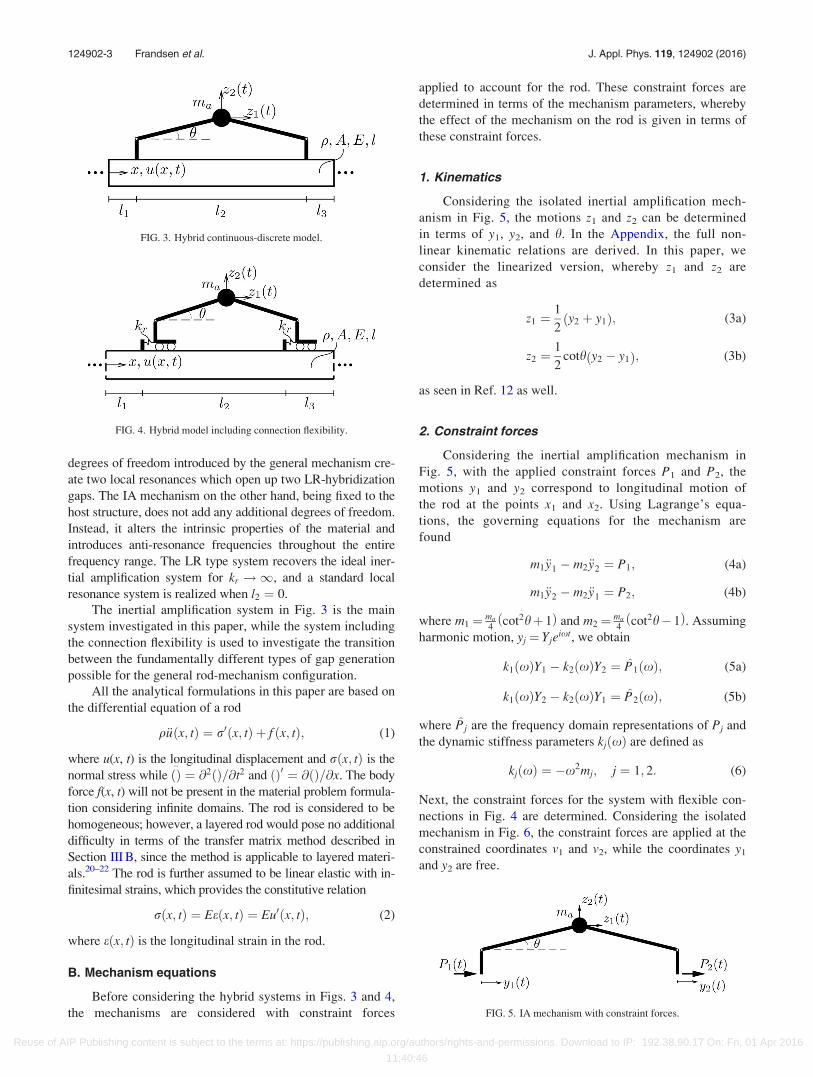
degrees of freedom introduced by the general mechanism cre-

ate two local resonances which open up two LR-hybridization

gaps. The IA mechanism on the other hand, being fixed to the

host structure, does not add any additional degrees of freedom.

Instead, it alters the intrinsic properties of the material and

introduces anti-resonance frequencies throughout the entire

frequency range. The LR type system recovers the ideal iner-

tial amplification system for kr !1, and a standard local

resonance system is realized when l2 ¼ 0.

The inertial amplification system in Fig. 3 is the main

system investigated in this paper, while the system including

the connection flexibility is used to investigate the transition

between the fundamentally different types of gap generation

possible for the general rod-mechanism configuration.

All the analytical formulations in this paper are based on

the differential equation of a rod

q€uðx; tÞ ¼ r0ðx; tÞ þ f ðx; tÞ; (1)

where u(x, t) is the longitudinal displacement and rðx; tÞ is the

normal stress while ðÞ::

¼ @2ðÞ=@t2 and ðÞ0 ¼ @ðÞ=@x. The body

force f(x, t) will not be present in the material problem formula-

tion considering infinite domains. The rod is considered to be

homogeneous; however, a layered rod would pose no additional

difficulty in terms of the transfer matrix method described in

Section III B, since the method is applicable to layered materi-

als.20–22 The rod is further assumed to be linear elastic with in-

finitesimal strains, which provides the constitutive relation

rðx; tÞ ¼ Eeðx; tÞ ¼ Eu0ðx; tÞ; (2)

where eðx; tÞ is the longitudinal strain in the rod.

B. Mechanism equations

Before considering the hybrid systems in Figs. 3 and 4,

the mechanisms are considered with constraint forces

applied to account for the rod. These constraint forces are

determined in terms of the mechanism parameters, whereby

the effect of the mechanism on the rod is given in terms of

these constraint forces.

1. Kinematics

Considering the isolated inertial amplification mech-

anism in Fig. 5, the motions z1 and z2 can be determined

in terms of y1, y2, and h. In the Appendix, the full non-

linear kinematic relations are derived. In this paper, we

consider the linearized version, whereby z1 and z2 are

determined as

z1 ¼1

2y2 þ y1ð Þ; (3a)

z2 ¼1

2coth y2 � y1ð Þ; (3b)

as seen in Ref. 12 as well.

2. Constraint forces

Considering the inertial amplification mechanism in

Fig. 5, with the applied constraint forces P1 and P2, the

motions y1 and y2 correspond to longitudinal motion of

the rod at the points x1 and x2. Using Lagrange’s equa-

tions, the governing equations for the mechanism are

found

m1€y1 � m2€y2 ¼ P1; (4a)

m1€y2 � m2€y1 ¼ P2; (4b)

where m1 ¼ ma

4cot2hþ 1ð Þ and m2 ¼ ma

4cot2h� 1ð Þ. Assuming

harmonic motion, yj ¼ Yjeixt, we obtain

k1ðxÞY1 � k2ðxÞY2 ¼ P̂1ðxÞ; (5a)

k1ðxÞY2 � k2ðxÞY1 ¼ P̂2ðxÞ; (5b)

where P̂j are the frequency domain representations of Pj and

the dynamic stiffness parameters kjðxÞ are defined as

kjðxÞ ¼ �x2mj; j ¼ 1; 2: (6)

Next, the constraint forces for the system with flexible con-

nections in Fig. 4 are determined. Considering the isolated

mechanism in Fig. 6, the constraint forces are applied at the

constrained coordinates v1 and v2, while the coordinates y1

and y2 are free.

FIG. 3. Hybrid continuous-discrete model.

FIG. 4. Hybrid model including connection flexibility.

FIG. 5. IA mechanism with constraint forces.

124902-3 Frandsen et al. J. Appl. Phys. 119, 124902 (2016)

Reuse of AIP Publishing content is subject to the terms at: https://publishing.aip.org/authors/rights-and-permissions. Download to IP: 192.38.90.17 On: Fri, 01 Apr 2016

11:40:46

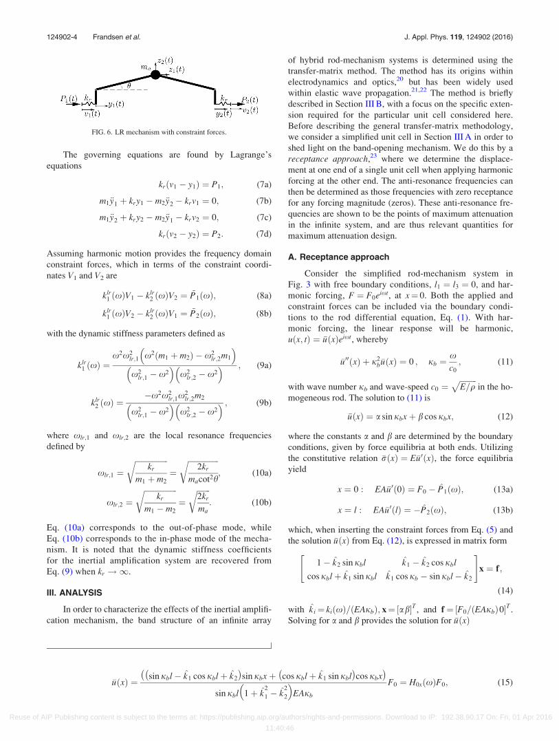
The governing equations are found by Lagrange’s

equations

krðv1 � y1Þ ¼ P1; (7a)

m1€y1 þ kry1 � m2€y2 � krv1 ¼ 0; (7b)

m1€y2 þ kry2 � m2€y1 � krv2 ¼ 0; (7c)

krðv2 � y2Þ ¼ P2: (7d)

Assuming harmonic motion provides the frequency domain

constraint forces, which in terms of the constraint coordi-

nates V1 and V2 are

klr1 ðxÞV1 � klr

2 ðxÞV2 ¼ ~P1ðxÞ; (8a)

klr1 ðxÞV2 � klr

2 ðxÞV1 ¼ ~P2ðxÞ; (8b)

with the dynamic stiffness parameters defined as

klr1 xð Þ ¼

x2x2lr;1 x2 m1 þ m2ð Þ � x2

lr;2m1

� �x2

lr;1 � x2� �

x2lr;2 � x2

� � ; (9a)

klr2 xð Þ ¼

�x2x2lr;1x

2lr;2m2

x2lr;1 � x2

� �x2

lr;2 � x2� � ; (9b)

where xlr;1 and xlr;2 are the local resonance frequencies

defined by

xlr;1 ¼ffiffiffiffiffiffiffiffiffiffiffiffiffiffiffiffiffi

kr

m1 þ m2

r¼

ffiffiffiffiffiffiffiffiffiffiffiffiffiffiffiffi2kr

macot2h

r; (10a)

xlr;2 ¼ffiffiffiffiffiffiffiffiffiffiffiffiffiffiffiffiffi

kr

m1 � m2

r¼

ffiffiffiffiffiffiffi2kr

ma

r: (10b)

Eq. (10a) corresponds to the out-of-phase mode, while

Eq. (10b) corresponds to the in-phase mode of the mecha-

nism. It is noted that the dynamic stiffness coefficients

for the inertial amplification system are recovered from

Eq. (9) when kr !1.

III. ANALYSIS

In order to characterize the effects of the inertial amplifi-

cation mechanism, the band structure of an infinite array

of hybrid rod-mechanism systems is determined using the

transfer-matrix method. The method has its origins within

electrodynamics and optics,20 but has been widely used

within elastic wave propagation.21,22 The method is briefly

described in Section III B, with a focus on the specific exten-

sion required for the particular unit cell considered here.

Before describing the general transfer-matrix methodology,

we consider a simplified unit cell in Section III A in order to

shed light on the band-opening mechanism. We do this by a

receptance approach,23 where we determine the displace-

ment at one end of a single unit cell when applying harmonic

forcing at the other end. The anti-resonance frequencies can

then be determined as those frequencies with zero receptance

for any forcing magnitude (zeros). These anti-resonance fre-

quencies are shown to be the points of maximum attenuation

in the infinite system, and are thus relevant quantities for

maximum attenuation design.

A. Receptance approach

Consider the simplified rod-mechanism system in

Fig. 3 with free boundary conditions, l1 ¼ l3 ¼ 0, and har-

monic forcing, F ¼ F0eixt, at x¼ 0. Both the applied and

constraint forces can be included via the boundary condi-

tions to the rod differential equation, Eq. (1). With har-

monic forcing, the linear response will be harmonic,

uðx; tÞ ¼ �uðxÞeixt, whereby

�u00 xð Þ þ j2b�u xð Þ ¼ 0 ; jb ¼

xc0

; (11)

with wave number jb and wave-speed c0 ¼ffiffiffiffiffiffiffiffiffiE=q

pin the ho-

mogeneous rod. The solution to (11) is

�uðxÞ ¼ a sin jbxþ b cos jbx; (12)

where the constants a and b are determined by the boundary

conditions, given by force equilibria at both ends. Utilizing

the constitutive relation �rðxÞ ¼ E�u0ðxÞ, the force equilibria

yield

x ¼ 0 : EA�u0ð0Þ ¼ F0 � P̂1ðxÞ; (13a)

x ¼ l : EA�u0ðlÞ ¼ �P̂2ðxÞ; (13b)

which, when inserting the constraint forces from Eq. (5) and

the solution �uðxÞ from Eq. (12), is expressed in matrix form

1� k̂2 sin jbl k̂1 � k̂2 cos jbl

cos jblþ k̂1 sin jbl k̂1 cos jb � sin jbl� k̂2

" #x ¼ f;

(14)

with k̂ i¼ kiðxÞ=ðEAjbÞ; x¼ ½ab�T , and f ¼ ½F0=ðEAjbÞ0�T .

Solving for a and b provides the solution for �uðxÞ

�u xð Þ ¼ sin jbl� k̂1 cos jblþ k̂2

� �sin jbxþ cos jblþ k̂1 sin jbl

� �cos jbx

� �sin jbl 1þ k̂

2

1 � k̂2

2

� �EAjb

F0 ¼ H0x xð ÞF0; (15)

FIG. 6. LR mechanism with constraint forces.

124902-4 Frandsen et al. J. Appl. Phys. 119, 124902 (2016)

Reuse of AIP Publishing content is subject to the terms at: https://publishing.aip.org/authors/rights-and-permissions. Download to IP: 192.38.90.17 On: Fri, 01 Apr 2016

11:40:46

where H0xðxÞ is the receptance function. The displacement

at x¼ l is given by

�u lð Þ ¼ 1þ k̂2 sin jbl

sin jbl 1þ k̂2

1 � k̂2

2

� �EAjb

F0 ¼ H0l xð ÞF0; (16)

whereby the anti-resonance frequencies can be determined

as the frequencies satisfying H0lðxÞ ¼ 0, i.e.,

k2ðxÞ sin jblþ EAjb ¼ 0: (17)

This transcendental equation is solved numerically for any

desired number of anti-resonance frequencies. The approxi-

mation for the first anti-resonance frequency is found in the

long-wavelength limit where sin jbl � jbl, i.e., in the sub-

Bragg regime. The approximation ~xa;1 is

�x2m2jblþ EAjb ¼ 0)

~xa;1 ¼

ffiffiffiffiffiffiffiffiffiffiEA=l

m2

s¼

ffiffiffiffiffiffiffiffiffiffiffiffiffiffiffiffiffiffiffiffiffiffiffiffiffiffiffiffiffiffiffiffiffiEA=l

ma cot2h� 1ð Þ=4

s; (18)

which is essentially the same as the anti-resonance frequency

of a discrete system as presented in Ref. 12 with effective

spring stiffness k ¼ EA=l. Hence, discretizing the rod as a

spring-mass system would provide the semi-infinite gap pre-

sented in the mentioned reference. The added complexity

from the rod is illustrated by the higher roots of Eq. (17) and

will be apparent from the band structures calculated in

Section IV.

B. Transfer matrix method

The transfer matrix method is based on relating the state

variables of a system across distances and interfaces, succes-

sively creating a matrix product from all the “sub” transfer

matrices, forming the cumulative transfer matrix.

Consider the hybrid continuous-discrete, rod-mechanism

system illustrated in Fig. 3, where the rod is modelled as a

continuum and the mechanism is modelled by discrete ele-

ments. The transfer matrix for the unit cell is based on the

host medium, i.e., the rod, representing the effects of the

mechanisms by point force matrices at x1 and x2. The state

variables for the rod are the longitudinal displacement u(x, t)and the normal stress rðx; tÞ. Dividing the system into three

layers separated at x1 and x2, the solution for the longitudinal

displacement in layer j can be written as a sum of forward

and backward travelling waves

ujðx; tÞ ¼ ðBðþÞj eijbx þ Bð�Þj e�ijbxÞeixt; (19)

where BðþÞj and B

ð�Þj are the amplitudes of the forward and

backward travelling waves. Using the linear elastic constitu-

tive relation for the stress, the state variables are expressed as

zjðxÞ ¼ujðxÞrjðxÞ

" #¼

1 1

Z �Z

" #BðþÞj eijbx

Bð�Þj e�ijbx

24

35

¼ HBðþÞj eijbx

Bð�Þj e�ijbx

24

35; (20)

thus defining the H-matrix, where Z ¼ iEjb. Relating the

state variables at either end of a homogeneous layer sepa-

rated by the distance lj yields

zRj ¼ H

eijblj 0

0 e�ijblj

" #BðþÞj eijbxj;L

Bð�Þj e�ijbxj;L

24

35

¼ HDj

BðþÞj eijbxj;L

Bð�Þj e�ijbxj;L

24

35; (21)

defining the “phase-matrix” Dj. The coordinate at the left

end of layer j is denoted xj;L. Solving Eq. (20) with zj ¼ zLj

for the vector of amplitudes and inserting into Eq. (21) define

the transfer matrix for layer j

zRj ¼ HDjH

�1zLj ¼ Tjz

Lj

Tj ¼cos jblj

1

Ejbsin jblj

�Ejb sin jblj cos jblj

264

375: (22)

Having defined the transfer matrices Tj, j¼ 1, 2, 3, we turn

to the constraint forces at the attachment points of the

mechanism.

We base our derivation of the point force matrices on a

frequency domain force equilibrium at the attachment points,

considering x1 first

ArL2 ¼ ArR

1 þ P̂1 ¼ ArR1 þ k1ðxÞuR

1 � k2ðxÞuR2 : (23)

It is noted that the force balance at point x1 depends on the

displacement at x2. Using the transfer matrix for layer 2, uR2

is expressed as

uR2 ¼ uL

2 cos jbl2 þrL

2

Ejbsin jbl2; (24)

which, along with the continuity requirement uR1 ¼ uL

2, yields

the force equilibrium

Aþ k2 xð ÞEjb

sinjbl2

� �rL

2 ¼ ArR1 þ k1 xð Þ�k2 xð Þcosjbl2ð ÞuR

1 ;

(25)

whereby the point force matrix, relating the state vector zL2 to

zR1 , can be identified

zL2 ¼

1 0

Ejb k1 xð Þ � k2 xð Þcos jbl2ð ÞAEjb þ k2 xð Þsin jbl2

AEjb

AEjb þ k2 xð Þsin jbl2

2664

3775

� zR1 ¼ P̂1zR

1 : (26)

Using a similar approach at point x2 provides the point force

matrix P̂2 as

P̂2 ¼1 0

k1 xð Þ � k2 xð Þcos jbl2A

1þ k2 xð ÞAEjb

sin jbl2

264

375; (27)

124902-5 Frandsen et al. J. Appl. Phys. 119, 124902 (2016)

Reuse of AIP Publishing content is subject to the terms at: https://publishing.aip.org/authors/rights-and-permissions. Download to IP: 192.38.90.17 On: Fri, 01 Apr 2016

11:40:46

which allows for relating the state vector at the right end of

the unit cell to the state vector at the left end through the cu-

mulative transfer matrix T

zR3 ¼ T3P̂2T2P̂1T1zL

1 ¼ TzL1 : (28)

The present framework is fully compatible with the local-

resonator-type system described in Section II by changing

the dynamic stiffness parameters in the point-force matrices

to those of Eq. (9), rather than those defined by Eq. (5).

Finally, it is noted that when the internal distance l2approaches zero, the point force matrices for the inertial

amplification system approach that of an attached point

mass, while the local-resonance point force matrices

approach that of an attached local resonator with resonance

frequency xlr;2 ¼ffiffiffiffiffiffiffiffiffiffiffiffiffiffi2kr=ma

p, recovering the expected limits.

With the cumulative transfer matrix for a unit cell deter-

mined, the Floquet-Bloch theorem for periodic structures24

is used to relate the state vector at either end through a phase

multiplier

zR3 ¼ zL

1eijl; (29)

where j ¼ jðxÞ is the wave number for the periodic mate-

rial and l is the unit-cell length. Combining Eqs. (28) and

(29) yields a frequency-dependent eigenvalue problem in eijl

ðT� eijlIÞzL1 ¼ 0; (30)

whereby the band structure of our periodic material system

is determined within a jðxÞ-formulation.

IV. BAND STRUCTURE

In this section, the band structure is calculated for the

systems in Figs. 3 and 4 as well as a standard local resonator

configuration, with primary focus on the inertial amplifica-

tion system. The mechanism is attached to an aluminum rod

with Young’s modulus E, density q, width b, height h, and

length l. These parameters are given in Table I along with

the equivalent mass and stiffness parameters mb and kb and

the first natural frequency xb.

The effect of the primary parameters of the system is

investigated, with special attention devoted to gap width and

depth. We begin by considering the case where the internal

length of the mechanism is equal to the unit-cell length, i.e.,

l1 ¼ l3 ¼ 0, illustrating the effect of the added mass ma, after

which we consider the effect of reducing the mechanism size

compared to the unit-cell length. Next, we consider the sys-

tem with flexible connections and the transition from local

resonance to ideal inertial amplification, after which we

compare the performance of the IA system to that of a

standard local resonator system where the resonator is

attached to the rod at a point within the unit cell.

A. Band structure and anti-resonance frequencies

We begin by considering a reference case, with the rod

parameters in Table I and the mechanism parameters given

in Table II.

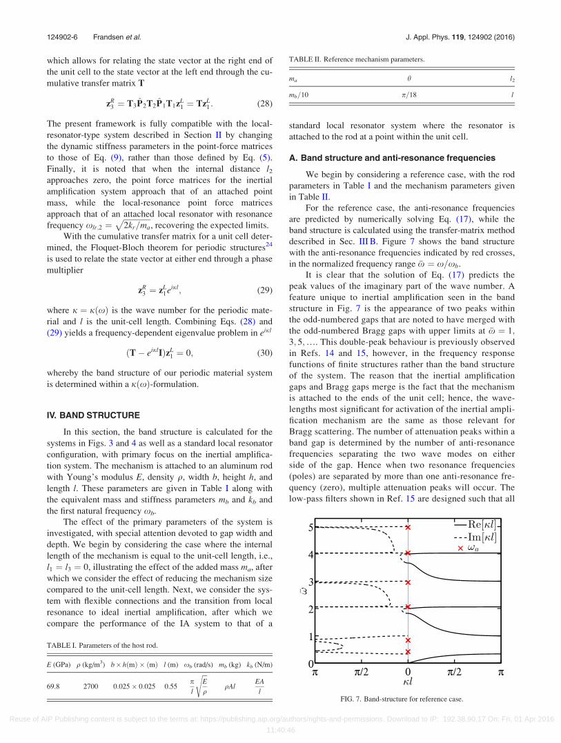
For the reference case, the anti-resonance frequencies

are predicted by numerically solving Eq. (17), while the

band structure is calculated using the transfer-matrix method

described in Sec. III B. Figure 7 shows the band structure

with the anti-resonance frequencies indicated by red crosses,

in the normalized frequency range �x ¼ x=xb.

It is clear that the solution of Eq. (17) predicts the

peak values of the imaginary part of the wave number. A

feature unique to inertial amplification seen in the band

structure in Fig. 7 is the appearance of two peaks within

the odd-numbered gaps that are noted to have merged with

the odd-numbered Bragg gaps with upper limits at �x ¼ 1;3; 5;…. This double-peak behaviour is previously observed

in Refs. 14 and 15, however, in the frequency response

functions of finite structures rather than the band structure

of the system. The reason that the inertial amplification

gaps and Bragg gaps merge is the fact that the mechanism

is attached to the ends of the unit cell; hence, the wave-

lengths most significant for activation of the inertial ampli-

fication mechanism are the same as those relevant for

Bragg scattering. The number of attenuation peaks within a

band gap is determined by the number of anti-resonance

frequencies separating the two wave modes on either

side of the gap. Hence when two resonance frequencies

(poles) are separated by more than one anti-resonance fre-

quency (zero), multiple attenuation peaks will occur. The

low-pass filters shown in Ref. 15 are designed such that all

TABLE I. Parameters of the host rod.

E (GPa) q (kg/m3) b� hðmÞ � ðmÞ l (m) xb (rad/s) mb (kg) kb (N/m)

69.8 2700 0:025� 0:025 0.55pl

ffiffiffiE

q

sqAl

EA

l

TABLE II. Reference mechanism parameters.

ma h l2

mb=10 p=18 l

FIG. 7. Band-structure for reference case.

124902-6 Frandsen et al. J. Appl. Phys. 119, 124902 (2016)

Reuse of AIP Publishing content is subject to the terms at: https://publishing.aip.org/authors/rights-and-permissions. Download to IP: 192.38.90.17 On: Fri, 01 Apr 2016

11:40:46

the anti-resonance frequencies are larger than the largest

resonance frequency, whereby the multiple peaks are all

found above the filter frequency. It is further noted that the

even gaps are of Bragg-type; however, they exhibit an

asymmetry, being distorted towards the double-peak gaps

which is also common when Bragg gaps are close to the

peak of local-resonance gaps.25,26

When considering the band structure for increasing fre-

quency, it appears that for higher band gaps, the anti-resonance

frequencies get further separated, increasing the gap width at

the cost of decreasing the gap depth. Furthermore, as the gap

widens, the anti-resonance frequencies approach the gap limits.

This indicates that the anti-resonance frequencies can be used

as a design-parameter for gap width. This is investigated fur-

ther in the Sec. IV C, where it is shown that this is only strictly

true for “full-length” mechanisms, i.e., when l1 ¼ l3 ¼ 0.

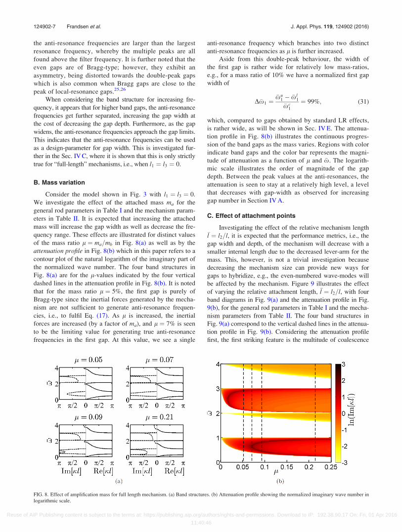
B. Mass variation

Consider the model shown in Fig. 3 with l1 ¼ l3 ¼ 0.

We investigate the effect of the attached mass ma for the

general rod parameters in Table I and the mechanism param-

eters in Table II. It is expected that increasing the attached

mass will increase the gap width as well as decrease the fre-

quency range. These effects are illustrated for distinct values

of the mass ratio l ¼ ma=mb in Fig. 8(a) as well as by the

attenuation profile in Fig. 8(b) which in this paper refers to a

contour plot of the natural logarithm of the imaginary part of

the normalized wave number. The four band structures in

Fig. 8(a) are for the l-values indicated by the four vertical

dashed lines in the attenuation profile in Fig. 8(b). It is noted

that for the mass ratio l ¼ 5%, the first gap is purely of

Bragg-type since the inertial forces generated by the mecha-

nism are not sufficient to generate anti-resonance frequen-

cies, i.e., to fulfil Eq. (17). As l is increased, the inertial

forces are increased (by a factor of ma), and l ¼ 7% is seen

to be the limiting value for generating true anti-resonance

frequencies in the first gap. At this value, we see a single

anti-resonance frequency which branches into two distinct

anti-resonance frequencies as l is further increased.

Aside from this double-peak behaviour, the width of

the first gap is rather wide for relatively low mass-ratios,

e.g., for a mass ratio of 10% we have a normalized first gap

width of

D�x1 ¼�xu

1 � �xl1

�xc1

¼ 99%; (31)

which, compared to gaps obtained by standard LR effects,

is rather wide, as will be shown in Sec. IV E. The attenua-

tion profile in Fig. 8(b) illustrates the continuous progres-

sion of the band gaps as the mass varies. Regions with color

indicate band gaps and the color bar represents the magni-

tude of attenuation as a function of l and �x. The logarith-

mic scale illustrates the order of magnitude of the gap

depth. Between the peak values at the anti-resonances, the

attenuation is seen to stay at a relatively high level, a level

that decreases with gap-width as observed for increasing

gap number in Section IV A.

C. Effect of attachment points

Investigating the effect of the relative mechanism length�l ¼ l2=l, it is expected that the performance metrics, i.e., the

gap width and depth, of the mechanism will decrease with a

smaller internal length due to the decreased lever-arm for the

mass. This, however, is not a trivial investigation because

decreasing the mechanism size can provide new ways for

gaps to hybridize, e.g., the even-numbered wave-modes will

be affected by the mechanism. Figure 9 illustrates the effect

of varying the relative attachment length, �l ¼ l2=l, with four

band diagrams in Fig. 9(a) and the attenuation profile in Fig.

9(b), for the general rod parameters in Table I and the mecha-

nism parameters from Table II. The four band structures in

Fig. 9(a) correspond to the vertical dashed lines in the attenua-

tion profile in Fig. 9(b). Considering the attenuation profile

first, the first striking feature is the multitude of coalescence

FIG. 8. Effect of amplification mass for full length mechanism. (a) Band structures. (b) Attenuation profile showing the normalized imaginary wave number in

logarithmic scale.

124902-7 Frandsen et al. J. Appl. Phys. 119, 124902 (2016)

Reuse of AIP Publishing content is subject to the terms at: https://publishing.aip.org/authors/rights-and-permissions. Download to IP: 192.38.90.17 On: Fri, 01 Apr 2016

11:40:46

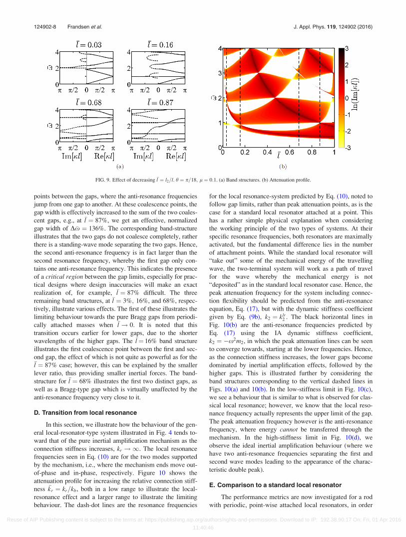
points between the gaps, where the anti-resonance frequencies

jump from one gap to another. At these coalescence points, the

gap width is effectively increased to the sum of the two coales-

cent gaps, e.g., at �l ¼ 87%, we get an effective, normalized

gap width of D�x ¼ 136%. The corresponding band-structure

illustrates that the two gaps do not coalesce completely, rather

there is a standing-wave mode separating the two gaps. Hence,

the second anti-resonance frequency is in fact larger than the

second resonance frequency, whereby the first gap only con-

tains one anti-resonance frequency. This indicates the presence

of a critical region between the gap limits, especially for prac-

tical designs where design inaccuracies will make an exact

realization of, for example, �l ¼ 87% difficult. The three

remaining band structures, at �l ¼ 3%; 16%, and 68%, respec-

tively, illustrate various effects. The first of these illustrates the

limiting behaviour towards the pure Bragg gaps from periodi-

cally attached masses when �l ! 0. It is noted that this

transition occurs earlier for lower gaps, due to the shorter

wavelengths of the higher gaps. The �l¼ 16% band structure

illustrates the first coalescence point between the first and sec-

ond gap, the effect of which is not quite as powerful as for the�l ¼ 87% case; however, this can be explained by the smaller

lever ratio, thus providing smaller inertial forces. The band-

structure for �l ¼ 68% illustrates the first two distinct gaps, as

well as a Bragg-type gap which is virtually unaffected by the

anti-resonance frequency very close to it.

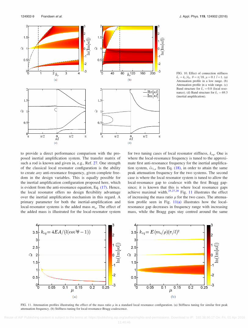
D. Transition from local resonance

In this section, we illustrate how the behaviour of the gen-

eral local-resonator-type system illustrated in Fig. 4 tends to-

ward that of the pure inertial amplification mechanism as the

connection stiffness increases, kr !1. The local resonance

frequencies seen in Eq. (10) are for the two modes supported

by the mechanism, i.e., where the mechanism ends move out-

of-phase and in-phase, respectively. Figure 10 shows the

attenuation profile for increasing the relative connection stiff-

ness �kr ¼ kr=kb, both in a low range to illustrate the local-

resonance effect and a larger range to illustrate the limiting

behaviour. The dash-dot lines are the resonance frequencies

for the local resonance-system predicted by Eq. (10), noted to

follow gap limits, rather than peak attenuation points, as is the

case for a standard local resonator attached at a point. This

has a rather simple physical explanation when considering

the working principle of the two types of systems. At their

specific resonance frequencies, both resonators are maximally

activated, but the fundamental difference lies in the number

of attachment points. While the standard local resonator will

“take out” some of the mechanical energy of the travelling

wave, the two-terminal system will work as a path of travel

for the wave whereby the mechanical energy is not

“deposited” as in the standard local resonator case. Hence, the

peak attenuation frequency for the system including connec-

tion flexibility should be predicted from the anti-resonance

equation, Eq. (17), but with the dynamic stiffness coefficient

given by Eq. (9b), k2 ¼ klr2 . The black horizontal lines in

Fig. 10(b) are the anti-resonance frequencies predicted by

Eq. (17) using the IA dynamic stiffness coefficient,

k2 ¼ �x2m2, in which the peak attenuation lines can be seen

to converge towards, starting at the lower frequencies. Hence,

as the connection stiffness increases, the lower gaps become

dominated by inertial amplification effects, followed by the

higher gaps. This is illustrated further by considering the

band structures corresponding to the vertical dashed lines in

Figs. 10(a) and 10(b). In the low-stiffness limit in Fig. 10(c),

we see a behaviour that is similar to what is observed for clas-

sical local resonance; however, we know that the local reso-

nance frequency actually represents the upper limit of the gap.

The peak attenuation frequency however is the anti-resonance

frequency, where energy cannot be transferred through the

mechanism. In the high-stiffness limit in Fig. 10(d), we

observe the ideal inertial amplification behaviour (where we

have two anti-resonance frequencies separating the first and

second wave modes leading to the appearance of the charac-

teristic double peak).

E. Comparison to a standard local resonator

The performance metrics are now investigated for a rod

with periodic, point-wise attached local resonators, in order

FIG. 9. Effect of decreasing �l ¼ l2=l. h ¼ p=18; l ¼ 0:1. (a) Band structures. (b) Attenuation profile.

124902-8 Frandsen et al. J. Appl. Phys. 119, 124902 (2016)

Reuse of AIP Publishing content is subject to the terms at: https://publishing.aip.org/authors/rights-and-permissions. Download to IP: 192.38.90.17 On: Fri, 01 Apr 2016

11:40:46

to provide a direct performance comparison with the pro-

posed inertial amplification system. The transfer matrix of

such a rod is known and given in, e.g., Ref. 27. One strength

of the classical local resonator configuration is the ability

to create any anti-resonance frequency, given complete free-

dom in the design variables. This is equally possible for

the inertial amplification configuration proposed here, which

is evident from the anti-resonance equation, Eq. (17). Hence,

the local resonator offers no design flexibility advantage

over the inertial amplification mechanism in this regard. A

primary parameter for both the inertial-amplification and

local-resonator systems is the added mass ma. The effect of

the added mass is illustrated for the local-resonator system

for two tuning cases of local resonator stiffness, keq. One is

where the local-resonance frequency is tuned to the approxi-

mate first anti-resonance frequency for the inertial amplifica-

tion system, ~x1;a from Eq. (18), in order to attain the same

peak attenuation frequency for the two systems. The second

case is where the local resonator system is tuned to allow the

local-resonance gap to coalesce with the first Bragg gap-

since; it is known that this is where local resonance gaps

achieve maximal width.25,27,28 Fig. 11 illustrates the effect

of increasing the mass ratio l for the two cases. The attenua-

tion profile seen in Fig. 11(a) illustrates how the local-

resonance gap decreases in frequency range with increasing

mass, while the Bragg gaps stay centred around the same

FIG. 10. Effect of connection stiffness�kr ¼ kr=kb. h¼ p=18; l¼ 0:1 �l¼1. (a)

Attenuation profile in a low range. (b)

Attenuation profile in a wide range. (c)

Band structure for �kr ¼ 0:8 (local reso-

nance). (d) Band structure for �kr ¼ 69:3(inertial amplification).

FIG. 11. Attenuation profiles illustrating the effect of the mass ratio l in a standard local resonance configuration. (a) Stiffness tuning for similar first peak

attenuation frequency. (b) Stiffness tuning for local-resonance-Bragg coalescence.

124902-9 Frandsen et al. J. Appl. Phys. 119, 124902 (2016)

Reuse of AIP Publishing content is subject to the terms at: https://publishing.aip.org/authors/rights-and-permissions. Download to IP: 192.38.90.17 On: Fri, 01 Apr 2016

11:40:46

frequency with mass increase. Comparing to the inertial

amplification system for l1 ¼ l3 ¼ 0, the inertial amplifica-

tion system is seen to perform better in terms of both gap

width and depth, see Fig. 8. The attenuation profile for local-

resonance-Bragg coalescence in Fig. 11(b) shows superior

gap width than seen for the local-resonance attenuation pro-

file in Fig. 11(a); however, the lowest and widest gap is cen-

tred around the first Bragg-gap frequency, thus not providing

any low-frequency attenuation. Furthermore, the inertial

amplification configuration still offers a wider and deeper

gap, while being lower in frequency.

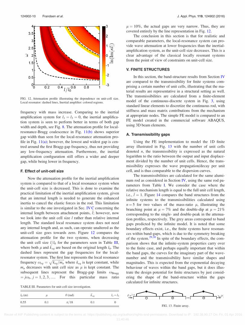
F. Effect of unit-cell size

Now the attenuation profile for the inertial amplification

system is compared to that of a local resonance system when

the unit-cell size is decreased. This is done to examine the

practical limitation of the inertial amplification system, given

that an internal length is needed to generate the enhanced

inertia to cancel the elastic forces in the rod. This limitation

is similar to the one investigated in Sec. IV C concerning the

internal length between attachment points, �l; however, now

we look into the unit cell size l rather than relative internal

length. The standard local resonance system does not need

any internal length and, as such, can operate unaltered as the

unit-cell size goes towards zero. Figure 12 compares the

attenuation profile for the two systems, when decreasing

the unit cell size l=l0 for the parameters seen in Table III,

where both l and �keq are based on the original length l0. The

dashed lines represent the gap frequencies for the local-

resonator system. The first line represents the local resonance

frequency xeq ¼ffiffiffiffiffiffiffiffiffiffiffiffiffiffikeq=ma

pwhere keq is kept constant, while

ma decreases with unit cell size as l is kept constant. The

subsequent lines represent the Bragg-gap limits xBragg

¼ jxb; j ¼ 1; 2; 3;…. For this particular mass ratio

l ¼ 10%, the actual gaps are very narrow. Thus, they are

covered entirely by the line representation in Fig. 12.

The conclusion in this section is that for realistic and

comparable parameters, the local-resonance system can pro-

vide wave attenuation at lower frequencies than the inertial-

amplification system, as the unit-cell size decreases. This is a

clear advantage of the classical locally resonant systems

from the point of view of constraints on unit-cell size.

V. FINITE STRUCTURES

In this section, the band-structure results from Section IV

are compared to the transmissibility for finite systems com-

prising a certain number of unit cells, illustrating that the ma-

terial results are representative in a structural setting as well.

The transmissibilities are calculated from a finite-element

model of the continuous-discrete system in Fig. 3, using

standard linear elements to discretize the continuous rod, with

stiffness and mass matrix contributions from the mechanism

at appropriate nodes. The simple FE model is compared to an

FE model created in the commercial software ABAQUS,

using 3D beam elements.

A. Transmissibility gaps

Using the FE implementation to model the 1D finite

array illustrated in Fig. 13 with the number of unit cells

denoted n, the transmissibility is expressed as the natural

logarithm to the ratio between the output and input displace-

ment divided by the number of unit cells. Hence, the trans-

missibility expresses the wave propagation/decay per unit

cell, and is thus comparable to the dispersion curves.

The transmissibilities are calculated for the same alumi-

num rod as considered in Section IV, using the same rod pa-

rameters from Table I. We consider the case where the

relative mechanism length is equal to the full unit cell length,

i.e., �l ¼ 1. Figure 14 compares the band structures from the

infinite systems to the transmissibilities calculated using

n¼ 5 for two values of the mass-ratio l, illustrating the

branching point at l ¼ 7% and the double-dip at l ¼ 21%

corresponding to the single- and double-peak in the attenua-

tion profiles, respectively. The grey areas correspond to band

gaps predicted by the infinite model. It is noted that some

boundary effects exist, i.e., the finite systems have resonan-

ces within band-gaps, which is due to the symmetry breaking

of the system.29,30 In spite of the boundary effects, the com-

parison shows that the infinite-system properties carry over

to the finite case, and perhaps equally important that within

the band gaps, the curves for the imaginary part of the wave-

number and the transmissibility have similar shapes and

magnitudes. This is expected from the exponential decaying

behaviour of waves within the band gaps, but it does illus-

trate the design potential for finite structures by just consid-

ering the shape of the band-structure within the gaps

calculated for infinite structures.

FIG. 12. Attenuation profile illustrating the dependence on unit-cell size.

Local resonator: dashed lines, Inertial amplifier: colored regions.

TABLE III. Parameters for unit-cell size investigation.

l0 (m) l h (rad) �keq l1¼ l3

0.55 0.1 p=18 0.1 0FIG. 13. Finite array.

124902-10 Frandsen et al. J. Appl. Phys. 119, 124902 (2016)

Reuse of AIP Publishing content is subject to the terms at: https://publishing.aip.org/authors/rights-and-permissions. Download to IP: 192.38.90.17 On: Fri, 01 Apr 2016

11:40:46

B. ABAQUS verification

The FE implementation of the hybrid rod-mechanism

system is tested against an implementation of the finite system

in the commercial FE-software ABAQUS. The ABAQUS

model is created as a 3D deformable “wire” model, using

three-dimensional beam elements for both rod and mecha-

nism. The mechanisms are distributed above and below the

main structure to have equal but opposite transverse force

components from the mechanisms. This is necessary to avoid

bending phenomena, and may easily be implemented in an ex-

perimental setting as well. The rigid connecting links are

modelled by assigning very large Young’s modulus and very

low density to the elements. The ideal connections are mod-

elled using translatory constraints to connect the rigid connec-

tors to the bar. Hence, the ABAQUS model is used to

illustrate the phenomena in a finite setting without obstructing

the results with, for the present purpose, unnecessary com-

plexities. Indeed, it is a subject of a future research paper to

investigate more realistic models of the physical configuration

in Fig. 2 both numerically and experimentally. The ABAQUS

model is created with the general rod parameters seen in

Table I and the general mechanism parameters h ¼ p=18 and�l ¼ 0:8. An illustration of the created ABAQUS model is

seen in Fig. 15(a).

Figure 15(b) shows the comparison between the trans-

missibilities calculated by the 1D FE implementation of the

rod-mechanism system and the 3D FE implementation in

ABAQUS, respectively, for the mass ratio l ¼ 10%.

Comparing both maximum attenuation frequencies and

gap limits, the transmissibility predicted by ABAQUS matches

rather well, especially for the first gap. Concerning the devia-

tions in the transmissibilities, it is worth considering the

case of gap-coalescence which, as seen in Fig. 9, is a rather

“singular” phenomena. As expected, using the “coalescence-

parameters” predicted by the analytical model does not cause

the gaps to coalesce in the 3D model. Figure 16 shows

the transmissibility comparison for the analytically predicted

coalescence-parameters and the ones found by inverse analysis

in ABAQUS. This pass band could be detrimental for design if

not taken into account, since the resonances are so closely

spaced. Hence, designing for gap-coalescence should be done

with care, as mentioned in Sec. IV C.

VI. CONCLUSIONS

We have investigated the wave characteristics of a con-

tinuous rod with a periodically attached inertial amplification

mechanism. The inertial amplification mechanism, which is

based on the same physical principles as the classical inerter,

creates band gaps within the dispersion curves of the underly-

ing continuous rod. The gap-opening mechanism is based on

an enhanced inertial force generated between two points in

the continuum, proportional to the relative acceleration

between these two points. An inertial amplification mecha-

nism has been used previously as a core building block for the

generation of a lattice medium, rather than serve as a light

attachment to a continuous structure as done here. Several

prominent effects are featured in the emerging band structure

of the hybrid rod-mechanism configuration. The anti-

FIG. 14. Comparison of band struc-

tures to transmissibilities for �l ¼ 1. (a)

Single peak behaviour. (b) Double

peak behaviour.

FIG. 15. (a) ABAQUS Model. (b) Comparison of 3D to 1D model. �l ¼ 0:8;l ¼ 0:1.

124902-11 Frandsen et al. J. Appl. Phys. 119, 124902 (2016)

Reuse of AIP Publishing content is subject to the terms at: https://publishing.aip.org/authors/rights-and-permissions. Download to IP: 192.38.90.17 On: Fri, 01 Apr 2016

11:40:46

FIG. 16. Transmissibility comparison for coalescence in 1D and 3D models for (a) l ¼ 0:06 and (b) l ¼ 0:07.

FIG. 17. Various band-gap opening mechanisms for constant mass ratio l ¼ 10% �l¼ 1. (a) Inertial amplification. (b) Local resonance. (c) Bragg scattering.

FIG. 18. Band structure for (a) pro-

posed inertially amplified rod with

l ¼ 10%, �l¼ 1 and (b) standard

locally resonant rod with l ¼ 204%.

The systems have almost equal-sized

gaps despite a factor of 20 difference

in added mass size.

124902-12 Frandsen et al. J. Appl. Phys. 119, 124902 (2016)

Reuse of AIP Publishing content is subject to the terms at: https://publishing.aip.org/authors/rights-and-permissions. Download to IP: 192.38.90.17 On: Fri, 01 Apr 2016

11:40:46

resonance frequencies are governed by both mechanism- and

rod-parameters. Hence, rather than a single anti-resonance fre-

quency, we see an infinite number (by virtue of the continuous

nature of the underlying rod), all of which can be predicted

for a simple choice of unit-cell parameters. For an example

choice of parameters, we illustrate the presence of multiple

attenuation peaks within the same gap. Furthermore, when

generalizing the parameters of the unit cell, we observe that

the anti-resonance frequencies can jump between gaps

whereby double-peak behaviour cannot be guaranteed for all

parameters. At the specific values of the anti-resonance jump,

band-gap coalescence emerges providing a very wide and

deep contiguous gap. This gap, however, is rather sensitive to

design and modelling inaccuracies.

In addition to these intriguing effects, we demonstrate

how attaching an inertial amplification mechanism to a con-

tinuous structure may be practically superior to attaching a

classical local resonator in that the former produces much

larger gaps for the same amount of added mass. Figure 17

compares the band structure of the proposed inertial amplifi-

cation system to those of a classical local resonator configu-

ration for two different tunings of the local resonator

stiffness keq. Figures 17(b) and 17(c) represent two cases of

stiffness tuning that provide a locally resonant band gap

(with equal central frequency) and a Bragg coalescence gap,

respectively. The central frequency is determined by solving

Eq. (17) numerically for the first two roots, xa;1 and xa;2.

The comparison illustrates that when the same mass is used,

the proposed concept achieves a first gap that is much wider

than what is obtainable by the classical local resonator con-

figuration, irrespective of the stiffness tuning for the local

resonator. In order to obtain comparable performance in

terms of band-gap width for the classical local-resonator sys-

tem, the added mass ma should be increased significantly.

Figure 18 compares similar gap widths for an inertial ampli-

fication system and a local resonance system. From the fig-

ure, we see that the inertial amplification system is superior

in terms of the magnitude of added mass, as the local reso-

nance system requires an approximately twenty times heav-

ier mass to obtain a comparable band-gap width (a mass that

is more than two times as heavy as the rod it is attached to).

The classical local resonator configuration, on the other

hand, faces less constraints on unit-cell size as demonstrated

in Fig. 12.

The presented concept of an inertially amplified continu-

ous structure opens a new promising avenue of band-gap

design. Potentially, it could be extended to surfaces of more

complex structures such as plates, shells, and membranes

leading to a general surface-coating design paradigm for

wave attenuation in structures. Steps toward achieving this

goal include a generalization of the formulation to admit

transverse vibrations, incorporation of frictional stiffness and

damping in the bearings of the mechanism, and generaliza-

tion to two dimensions.

ACKNOWLEDGMENTS

Niels M. M. Frandsen and Jakob S. Jensen were

supported by ERC starting Grant No. 279529 INNODYN.

Osama R. Bilal and Mahmoud I. Hussein were supported by

the National Science Foundation Grant No. 1131802.

Further, N.M.M.F would like to extend his thanks to the

foundations: COWIfonden, Augustinusfonden, Hede Nielsen

Fonden, Ingeniør Alexandre Haymnan og Hustrus Fond,

Oticon Fonden and Otto Mønsted Fonden. All authors are

grateful to graduate student Dimitri Krattiger for his

assistance in generating the image of Figure 1.

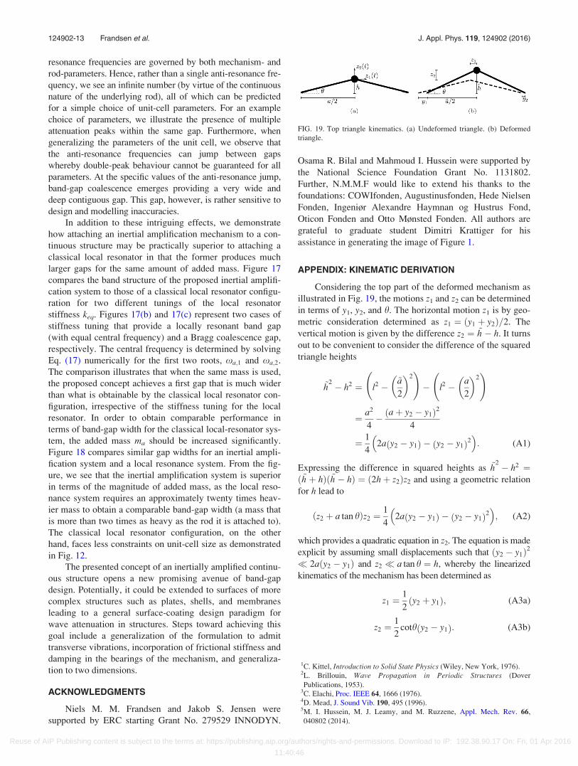
APPENDIX: KINEMATIC DERIVATION

Considering the top part of the deformed mechanism as

illustrated in Fig. 19, the motions z1 and z2 can be determined

in terms of y1, y2, and h. The horizontal motion z1 is by geo-

metric consideration determined as z1 ¼ ðy1 þ y2Þ=2. The

vertical motion is given by the difference z2 ¼ ~h � h. It turns

out to be convenient to consider the difference of the squared

triangle heights

~h2 � h2 ¼ l2 � ~a

2

� �2 !

� l2 � a

2

� �2 !

¼ a2

4� aþ y2 � y1ð Þ2

4

¼ 1

42a y2 � y1ð Þ � y2 � y1ð Þ2� �

: (A1)

Expressing the difference in squared heights as ~h2 � h2 ¼

ð~h þ hÞð~h � hÞ ¼ ð2hþ z2Þz2 and using a geometric relation

for h lead to

z2 þ a tan hð Þz2 ¼1

42a y2 � y1ð Þ � y2 � y1ð Þ2� �

; (A2)

which provides a quadratic equation in z2. The equation is made

explicit by assuming small displacements such that ðy2 � y1Þ2� 2aðy2 � y1Þ and z2 � a tan h ¼ h, whereby the linearized

kinematics of the mechanism has been determined as

z1 ¼1

2y2 þ y1ð Þ; (A3a)

z2 ¼1

2coth y2 � y1ð Þ: (A3b)

1C. Kittel, Introduction to Solid State Physics (Wiley, New York, 1976).2L. Brillouin, Wave Propagation in Periodic Structures (Dover

Publications, 1953).3C. Elachi, Proc. IEEE 64, 1666 (1976).4D. Mead, J. Sound Vib. 190, 495 (1996).5M. I. Hussein, M. J. Leamy, and M. Ruzzene, Appl. Mech. Rev. 66,

040802 (2014).

FIG. 19. Top triangle kinematics. (a) Undeformed triangle. (b) Deformed

triangle.

124902-13 Frandsen et al. J. Appl. Phys. 119, 124902 (2016)

Reuse of AIP Publishing content is subject to the terms at: https://publishing.aip.org/authors/rights-and-permissions. Download to IP: 192.38.90.17 On: Fri, 01 Apr 2016

11:40:46

6H. Frahm, “Device for damping vibration of bodies,” U.S. Patent

989,958A (1911).7Z. Liu, X. Zhang, Y. Mao, Y. Y. Zhu, Z. Yang, C. T. Chan, and P. Sheng,

Science 289, 1734 (2000).8D. Yu, Y. Liu, G. Wang, L. Cai, and J. Qiu, Phys. Lett. A 348, 410 (2006).9D. Yu, Y. Liu, G. Wang, H. Zhao, and J. Qiu, J. Appl. Phys. 100, 124901

(2006).10Y. Pennec, B. Djafari-Rouhani, H. Larabi, J. O. Vasseur, and A. C.

Hladky-Hennion, Phys. Rev. B 78, 104105 (2008).11T.-T. Wu, Z.-G. Huang, T.-C. Tsai, and T.-C. Wu, Appl. Phys. Lett. 93,

111902 (2008).12C. Yilmaz, G. M. Hulbert, and N. Kikuchi, Phys. Rev. B 76, 054309 (2007).13C. Yilmaz and G. Hulbert, Phys. Lett. A 374, 3576 (2010).14G. Acar and C. Yilmaz, J. Sound Vib. 332, 6389 (2013).15C. Yilmaz and N. Kikuchi, J. Sound Vib. 293, 171 (2006).16M. C. Smith, IEEE Trans. Autom. Control 47, 1648 (2002).17M. Z. Q. Chen, C. Papageorgiou, F. Scheibe, F. C. Wang, and M. Smith,

IEEE Circuits Syst. Mag. 9, 10 (2009).18O. Yuksel and C. Yilmaz, J. Sound Vib. 355, 232 (2015).

19C. Papageorgiou, N. E. Houghton, and M. C. Smith, J. Dyn. Syst., Meas.,

Control 131, 011001 (2009).20W. L. Mochan, M. d. C. Mussot, and R. G. Barrera, Phys. Rev. B 35, 1088

(1987).21R. Esquivel-Sirvent and G. H. Cocoletzi, J. Acoust. Soc. Am. 95, 86

(1994).22M. I. Hussein, G. M. Hulbert, and R. A. Scott, J. Sound Vib. 289, 779

(2006).23R. E. D. Bishop, The Mechanics of Vibration (Cambridge University

Press, 1979).24F. Bloch, Z. Phys. 52, 555 (1929).25Y. Xiao, B. R. Mace, J. Wen, and X. Wen, Phys. Lett. A 375, 1485

(2011).26L. Liu and M. I. Hussein, J. Appl. Mech. 79, 011003 (2012).27R. Khajehtourian and M. I. Hussein, AIP Adv. 4(12), 124308 (2014).28Y. Xiao, J. Wen, and X. Wen, New J. Phys. 14, 033042 (2012).29B. Djafari-Rouhani, L. Dobrzynski, O. H. Duparc, R. E. Camley, and A.

A. Maradudin, Phys. Rev. B 28(4), 1711 (1983).30J. S. Jensen, J. Sound Vib. 266, 1053 (2003).

124902-14 Frandsen et al. J. Appl. Phys. 119, 124902 (2016)

Reuse of AIP Publishing content is subject to the terms at: https://publishing.aip.org/authors/rights-and-permissions. Download to IP: 192.38.90.17 On: Fri, 01 Apr 2016

11:40:46