0

Individual political contributions and firm performance

Alexei V. Ovtchinnikov*

Owen Graduate School of Management

Vanderbilt University

alexei.ovtchinnikov@owen.vanderbilt.edu

and

Eva Pantaleoni

Vanderbilt Kennedy Center

Vanderbilt University

eva.pantaleoni@vanderbilt.edu

Abstract

We present evidence that individuals make political contributions strategically by targeting politicians

with power to affect their economic well-being. Individuals in Congressional districts with greater

industry clustering tend to support politicians with jurisdiction over the industry. The effect is stronger

for Congressional committees with jurisdiction over more concentrated industries, in states with more

concentrated industries and in states with higher unemployment. Individual political contributions are

also associated with improvements in operating performance of firms in industry clusters. The relation

between contributions and firm performance is strongest for poorly performing firms, firms closer to

financial distress, and for contributions in close elections. The results imply that individual political

contributions are valuable to firms, especially during bad economic times.

JEL classifications: G30, G33, G38

Keywords: Political contributions, firm performance, firm value

December 30, 2010

* Corresponding author. Please send correspondence to the Owen Graduate School of Management, 401 21

st

Avenue, South, Nashville, TN 37203.

1

Individual political contributions and firm performance

Abstract

We present evidence that individuals make political contributions strategically by targeting politicians

with power to affect their economic well-being. Individuals in Congressional districts with greater

industry clustering tend to support politicians with jurisdiction over the industry. The effect is stronger

for Congressional committees with jurisdiction over more concentrated industries, in states with more

concentrated industries and in states with higher unemployment. Individual political contributions are

also associated with improvements in operating performance of firms in industry clusters. The relation

between contributions and firm performance is strongest for poorly performing firms, firms closer to

financial distress, and for contributions in close elections. The results imply that individual political

contributions are valuable to firms, especially during bad economic times.

1

Individual political contributions and firm performance

1. Introduction

A growing body of research finds that firms establish specific connections with politicians.

These connections are often broken into explicit connections that arise when a politician joins the firm or

its board of directors (or vice versa) and into implicit connections that arise when a firm makes political

contributions to the candidate’s (re)election campaign (Masters and Keim (1985), Zardkoohi (1985),

Grier, Munger, and Roberts (1994), Kroszner and Stratmann (1998), Kroszner and Stratmann (2005),

Faccio (2006), Goldman, Rocholl, and So (2009), and Cooper, Gulen, and Ovtchinnikov (2010)).

Researchers also document that political connections are valuable (Fisman (2001), Faccio (2006), Faccio

and Parsley (2009), Goldman, Rocholl, and So (2009), Cooper, Gulen, and Ovtchinnikov (2010), for

example).1

Firms are obviously impacted by government policy, so the desire to establish connections with

politicians may seem logical. These firms do not operate in a vacuum, however, so any government

decision that significantly impacts them is also likely to impact the surrounding community. If this is

true, it is not unreasonable to argue that different firm stakeholders would also have a vested interest in

the political process and should try to affect government decisions on behalf of the firm. If successful,

these efforts, in turn, should have a positive impact on the firm.

Consider the April 2010 BP oil spill in the Gulf of Mexico, for example. The spill led to a

temporary government moratorium on deepwater drilling, which, in turn, has had a significantly negative

impact on the surrounding communities that support the oil drilling industry. According to industry

experts, every job on an oil rig translates into four or more jobs to service and support it. These include

people manufacturing the equipment, delivering it to the platform, and feeding the rig crews (Adams

(2010)).2 Adams (2010), citing data from the Louisiana Mid-Continent Oil and Gas Association, reports

further that the moratorium decision erased at least $165 million in monthly wages from businesses that

support the oil drilling industry. In response to the government’s decision, close to 11,000 people took it

to the streets in protests arguing that the moratorium decision could damage the region even more that the

oil spill itself.

This example illustrates that individuals understand their economic dependency on nearby firms

and exercise their right to lobby the government. In addition to organized protests, individuals may also

exercise the power of their votes (as they did in the November 2010 mid-term election) and the power of

their wallet. The latter tactic may be especially effective if the goal is to reach non-local politicians

1 Some papers find that political connections destroy value. See Aggarwal, Meschke, and Wang (2009), for

example. 2 Adams, Russell, 2010. “The Gulf Oil Spill: Drill Ban Hits Service Firms.” The Wall Street Journal, July 22, 2010.

2

(something that cannot be accomplished with votes) and if the costs of organized protests relative to the

expected benefits are high.

The purpose of this paper is to empirically investigate whether individuals do in fact use the

power of their wallet and make political contributions strategically with their economic interests in mind.

We should certainly expect individuals to pursue a variety of motives when making political

contributions, such as ideological, partisan, access-seeking, or identity-based (Francia, Green, Herrnson,

Powell, and Wilcox (2003)). We ask whether individuals are also strategic, specifically whether they

have their economic livelihood in mind when deciding which politician to support. The answer in the

affirmative naturally begs a question of what effect, if any, individual political contribution efforts have

on the performance of the nearby firms. The position that we take in this paper, therefore, is that

individual political contributions are, at least in part, investment in political capital.

Numerous papers report evidence consistent with the view that contributions represent an

investment in political capital. Incumbent politicians who are party leaders, committee chairs, or

members of powerful committees raise more money (Grier and Munger (1991), Romer and Snyder

(1994), Milyo (1997)). Snyder (1992) shows that political contributions are persistent and argues that it is

consistent with the view that contributors establish long-term investment relationships with politicians.

Conversely, politicians who change committees or retire experience a drop in the financial support from

previous contributors (Romer and Snyder (1994), Kroszner and Stratmann (1998)). A parallel line of

research analyzes political contributor characteristics and finds that variables that capture the severity of

the free-rider problem faced by the contributor and variables that capture the closeness of the relationship

between the contributor and the government help determine the contributor’s propensity to participate in

the political process (Masters and Keim (1985), Zardkoohi (1985), and Grier, Munger, and Roberts

(1994)). Finally, several papers report evidence that politicians trade favors, such as policy decisions, for

contributions. Stratmann (2002), for example, finds that politicians are willing to switch their votes based

on political contributions received. Consistent with this view, Stratmann (1998) finds that political

contributions cluster in time around relevant Congressional votes. The prospect that politicians exchange

favors for votes is also present in Prat (2002), Coate (2004), and Ashworth (2006).

Figure 1 hints that individuals are in fact strategic and contribute in times when their economic

livelihood is at stake. Panels A and B show total political contributions made by Microsoft and by

residents in the Microsoft’s Congressional district during the firm’s antitrust litigation with the

Department of Justice. That Microsoft’s political contributions increase significantly during the antitrust

litigation is not surprising considering the impact that a negative verdict would have had on the firm.

What is perhaps more surprising but consistent with our argument, is the significant increase in

contributions from individuals in the Microsoft’s district over the same time period. The spikes in

3

individual contributions around important decision dates are quite evident in panel B. Individuals on

average contribute twice as much during each month of the trial period compared to any other period.

This translates into $4.4 million in total individual political contributions during the trial period compared

to $2.8 million during all other months combined. Thus, there is a visibly disproportionate political

participation from individuals residing close to Microsoft during the firm’s antitrust trial.

Our methodology builds on this example. We use the geographic clustering of industries in the

U.S. to identify Congressional districts (CDs) in which individuals are especially economically dependent

on the nearby firms. We then identify all Congressional committees in the House of Representatives and

the Senate that have jurisdictional authority over the local industry clusters. Politicians serving on these

committees are identified as “economically relevant” for individuals residing in the “economically

dependent” Congressional districts. Our strategy, therefore, is to match politicians with Congressional

districts based on the power of politicians to affect the economic livelihood of individuals in the district.

We first analyze whether individuals in economically dependent CDs have a greater tendency to

make political contributions to economically relevant politicians. To pin down the effect, we follow a

three-step approach. We first document a significantly higher propensity of economically dependent CDs

to make political contributions to economically relevant politicians in the overall sample. We then

subject our analysis to a number of robustness tests which, when considered together, allow us to make a

stronger statement about the individual propensity to support economically relevant politicians. Third, we

perform a number of subsample analyses to further rule out alternative explanations for our baseline

results.

In the first step, we estimate a series of CD and politician fixed effects regressions and document

a significantly higher propensity of economically dependent CDs to make political contributions to

economically relevant politicians. In particular, we estimate logit, poisson, and tobit regressions and find

that political contributions are more likely, more frequent, and of higher amount when made from

economically dependent CDs to economically relevant politicians. We measure the extent to which a CD

is economically dependent with the number of firms under the politician’s jurisdiction, the total assets of

these firms, and the total employees of these firms and find that all three measures are positively and

significantly related to the CD contribution intensity.

A potential concern with our results is that they may simply reflect the local constituency effect.

In other words, it may be the case that politicians from economically dependent CDs are picked to serve

on economically relevant committees. Local constituents choose to support their own politicians, which

gives rise to the positive relation between the CD economic dependence status and its contribution

intensity to economically relevant politicians. We explicitly control for whether the economically

relevant politician is local to the economically dependent CD and find that it does not affect our results.

4

Non-local economically dependent politicians are just as likely to receive political contributions from

economically dependent CDs and receive contributions more often and of higher amounts than other

politicians. It is also important to note that the majority of the politician’s campaign financing comes

from non-local CDs (Gimpel, Lee, and Pearson-Merkowitz (2008). We confirm this result and find that

the distance between the politician’s own CD and the contributing CD is actually inversely related to the

amount of contributions pledged. This also helps alleviate a concern that political contributions are

substitutes for votes that economically dependent contributors can pledge to economically relevant

politicians.

Our regression methodology focuses on the within-CD and the within-politician variation in the

political contribution intensity, so our results are robust to all CD-level and all politician-level

confounding covariates. In the second step, we verify that our results are also robust to a variety of

alternative specifications that target different time periods and different subsamples of firms, as well as to

specifications that control for the local constituency effect and to specifications that control for corporate

political contributions. This last control is especially relevant because it implies that are results are not

driven by firms simply encouraging their own employees to make political contributions on behalf of the

firms. We also note that the majority of CDs in our sample contain no firms that are political active

themselves, which suggests that the effect that we identify is largely orthogonal to the corporate political

activism identified in previous studies (Cooper, Gulen, and Ovtchinnikov (2010), for example).

We recognize, however, that the set of potential omitted variables is infinite, so our robustness

checks that include additional controls can only go so far. Thus, in the third step, we change our strategy

and carry out a number of subsample analyses. Specifically, our strategy is to focus on subsamples of

CDs and politicians for which the expected likelihood of making and receiving political contributions is

stronger under our hypothesis but absent if the results are driven by an omitted variable. We find a higher

propensity of economically dependent CDs to make political contributions to politicians who serve on

Congressional committees with jurisdictions over more geographically focused industries. We also find a

higher contribution propensity in states with more concentrated industries. These results provide further

credence to our hypothesis since individuals residing nearby major industry clusters are more

economically impacted by local firms and, therefore, should have a greater need to make political

contributions to economically relevant politicians. Lastly, we find a higher propensity of economically

dependent CDs to make political contributions to economically relevant politicians in states with high

unemployment. We interpret this evidence as also consistent with our hypothesis considering that the

individuals’ need to lobby government officials should be especially high during bad economic times.

To get a sense for the economic significance of the effect, we sort all CDs in deciles based on the

number of firms under the politician’s jurisdiction, the total assets of these firms, and the total employees

5

of these firms and define the most and least economically dependent CDs as those in the top and bottom

deciles of each sort, respectively. Depending on the economic dependence measure used, the most

economically dependent CDs contribute between $152.9 million and $172.3 million to all economically

relevant politicians over our sample period. In contrast, the least economically dependent CDs contribute

between $69.9 million and $84.9 million to those politicians. Thus, compared to the least economically

dependent CDs, the most economically dependent CDs contribute twice as much to economically relevant

politicians.

Given this evidence, we next proceed to analyzing operating performance of firms located in

economically dependent CDs. If individuals derive their economic livelihood from nearby firms and,

therefore, make political contributions on behalf of these firms and if politicians do exchange policy

favors for contributions, we expect a positive relation between political contributions from economically

dependent CDs to economically relevant politicians and firm performance. As in the previous analysis,

we proceed in multiple steps. We start by documenting a strong positive relation between political

contributions from economically dependent CDs to economically relevant politicians and future operating

performance of firms located in economically dependent CDs. We then attempt to tackle reverse

causality by identifying situations when the relation between political contributions and firm performance

should be stronger under our explanation but absent or of the reverse sign under the reverse causality

explanation. Finally, we set the bar significantly higher and look for an exogenous shock to the CD

economic dependence status. We then analyze how individual political contributions adjust to this shock

and what impact, if any, these adjustments have on future firm performance.

In the first step of our analysis, we estimate a series of regressions that relate individual political

contributions to future changes in firm operating performance. We obtain operating performance data for

all firms located in economically dependent CDs and show that future operating performance changes are

positively and significantly related to the frequency and the amount of political contributions made from

economically dependent CDs to economically relevant politicians. Interestingly, future performance

changes are unrelated to contributions made to politicians who are not economically relevant. We obtain

these results in regressions of industry-adjusted ROA changes and market-to-book changes after

controlling for other determinants of future performance.

The regression results allow us to comment on correlations but not causality. Reverse causality is

a serious issue in our regressions. It well may be the case that political contributions are a form of a

normal consumption good, so individuals make more political contributions when firms and nearby

residents are doing well. To tackle this issue, we perform two additional tests. First, we carry out a

number of subsample analyses. We look for subsamples when the relation between political contributions

and firm performance should be stronger under our hypothesis but absent or of the reverse sign under the

6

reverse causality explanation. We find that the positive relation between political contributions to

economically relevant politicians and firm performance is stronger for poorly performing firms and firms

closer to financial distress. This evidence is consistent with our hypothesis since the incentive to lobby

government officials and the expected payoffs from this activity are highest during bad economic times.

Note that under the reverse causality, we expect that it is the well-performing firms that exhibit the

strongest relation between political contributions and firm performance. Instead, we find the opposite.

We also find that the positive relation between political contributions to economically relevant politicians

and firm performance is strongest when contributions are made in close (re)election races. We again

interpret this evidence as consistent with our hypothesis as the marginal dollar of contributions matters

more to a politician in a close race against a strong opponent. Hence, politicians in close races should be

more willing to trade favors for contributions. It is difficult to interpret this result under the reverse

causality explanation, which would require that individuals residing nearby well-performing firms are for

some reason compelled to contribute more to politicians but only in close races.

Our second test focuses on an exogenous shock to the CD economic dependence status and on the

impact of this shock on individual political contribution practices and future firm performance. We

consider mergers between bidders and targets that operate in different industries and in different

locations. Such mergers create a new set of economically relevant politicians for individuals residing in

the bidder and the target CD, so it is natural to ask whether individuals alter their contribution practices

and increase their support of the newly created economically relevant politicians. We find evidence

consistent with this assertion. Even though contributions to all politicians increase from before to after

the merger, there is a significantly more pronounced increase in contributions from the bidder CDs to

politicians who are economically relevant for the targets and from the target CDs to politicians who are

economically relevant for the bidders. The former contributions increase by 95 percent from before to

after the merger, while the latter contributions increase by 57 percent. In comparison, contributions from

the target CDs to target politicians and from the bidder CDs to bidder politicians increase by 52 percent

and 28 percent, respectively.

Finally, we find that contributions from the target CDs to bidder politicians have no impact on

bidder operating performance prior to the merger and a significantly positive impact after the merger.

Similarly, contributions from the bidder CDs to target politicians have no impact on bidder performance

prior to the merger and a positive impact after the merger. These results are consistent with our

hypothesis that individuals change their contribution decisions in response to an exogenous shock to their

economic dependence status. In turn, these new contributions become relevant for firm performance.

Overall, the results in this paper suggest that individuals make political contributions

strategically, with their economic livelihood in mind. These contributions also appear to be valuable to

7

firms in the sense that they are related to firm performance. The results in this paper are important for

several reasons. First, we provide an important contribution to the literature on political connections. We

show that not only firms establish political connections to gain access to politicians, but also individuals

whose economic livelihood is dependent on politicians make contributions strategically with their

economic interests in mind. These contributions are also valuable to firms. One question that we do not

comment on in this paper is how precisely political contributions generate value. We rely on previous

literature and assume that political contributions matter because politicians care about reelection and need

campaign financing to win. Thus, politicians are willing to trade favorable decisions for political

contributions. Numerous papers present evidence consistent with this view, but inferences are often

difficult because of endogeneity and other methodological concerns (see Ansolabehere, et al (2003) and

Stratmann (2005) for excellent reviews). The results in this paper imply that contributors get value from

their contributions, which is suggestive of quid pro quo arrangements between contributors and

politicians.

Our second contribution is to the literature on geographic location and firm decision making.

Numerous papers report evidence that geography matters for firm behavior (Gaspar and Massa (2007),

Becker, Cronqvist, and Fahlenbrach (2010), Becker, Ivkovic, and Weisbenner (2010), Francis, Hasan,

John, and Waismann (2007), Hilary and Hui (2009), John, Knyazeva, and Knyazeva (2010), to name a

few). The results in this paper also demonstrate that geography matters to firms. The channel that we

identify here stems from the economic dependency of individuals on nearby firms. Because of this

dependency, individuals make political contribution decisions that benefit firms and the contributing

individuals. So, unlike prior hypotheses that are mostly built around the view that geographic

characteristics influence firm decision making, our hypothesis runs in the opposite direction. It is firm

characteristics that affect the surrounding public’s decisions. These decisions, in turn, have positive

spillover effects on the nearby firms.

The rest of the paper is organized as follows. Section 2 describes our data sources and variable

construction. Section 3 presents evidence that individuals strategically choose to contribute money to

economically relevant politicians. Section 4 presents evidence that contributions to economically relevant

politicians are associated with improvements in future firm performance. Section 5 concludes.

2. Data sources and variable construction

2.1. Data

Our sample consists of all individual hard money political contributions to candidates for

Congress for the period January 1991 – December 2008. We obtain contributions data from the Federal

Election Commission (FEC) detailed individual contributions file which contains all individual

8

contributions in excess of $200. The file includes information on (i) the name and address of the

contributing individual, (ii) the identity of the receiving candidate and/or committee, and (iii) the date and

the amount of the individual contribution. The original dataset includes 9,314,217 contributions from

individuals over our sample period. After deleting individual contributions to non-candidate committees

(i.e. contributions to corporate and non-corporate political action committees (PACs) and contributions to

national party committees), we are left with 4,874,994 contributions made to 8,302 unique political

candidates running for office from all Congressional Districts (CDs). We merge this file with the FEC

candidate summary file to obtain information on (i) the candidate’s sought after office, (ii) the

incumbency status, (iii) the candidate’s party affiliation, (iv) the CD that the candidate represents, and (v)

the election outcome. For all elected officials, we further obtain data on their committee assignments and

their party rankings on each serving committee. This data is from Charles Stewart’s Congressional Data

Page.3

We first assign all individual contributions to their respective CDs using zip code data as follows.

The Census Bureau provides cartographic CD boundary files for every election cycle starting with the

103rd

Congress (January 1993 – January 1995). The size and shape of each CD are established by each

state, and are based on the population data provided decennially by the Census Bureau. In our sample,

the CDs for the 103rd

Congress were the first to reflect the redistricting based on the 1990 Census. The

CDs for the 108th Congress (January 2003 to January 2005) were the first to reflect the redistricting based

on the 2000 Census. In addition to decennial redistricting, several other intra-decennial redistricting

decisions were made over our sample period, so we obtain CD boundaries data for every election cycle in

our sample.4 The Census Bureau also provides cartographic zip code boundary files, but unlike the CD

boundary data, the zip code boundary data is available only for 2000. We assume that zip codes remain

fixed for the duration of our sample, an assumption that biases us against finding any results, and use a

geographic information system (GIS) to calculate the latitude and longitude of the geographic center of

each CD and each zip code in the U.S. Zip codes are assigned to a CD if their geographic center falls

with the CD boundary. Further details of this procedure are described in Appendix A.

Figure 2 maps individual contribution totals by CD over our sample period. Two results stand

out. First, there appears significant heterogeneity in political contributions across CDs. Contribution

totals range from $905,069 for the 31st district in Texas (a strip in central Texas from north Austin to

Stephenville) to $101.5 million for the 14th district in New York (Manhattan east side, Roosevelt Island,

3 We thank Charles Stewart III for generously providing this data on his website

http://web.mit.edu/17.251/www/data_page.html. 4 In the 104

th Congress, six states were redistricted: Georgia, Louisiana, Maine, Minnesota, South Carolina, and

Virginia. In the 105th

Congress, five states were redistricted: Florida, Georgia, Kentucky, Louisiana, and Texas. In

the 106th

Congress, three states were redistricted: New York, North Carolina, and Virginia.

9

and neighborhoods of Astoria, Long Island City, and Sunnyside in Queens). Second, political

contributions cluster in small geographic areas. The ten CDs with the highest contributions are New

York’s 14th district ($101.5 million), District of Columbia (DC) ($93.1 million), New York’s 8

th district

($57.5 million), Virginia’s 8th district ($56.8 million), Maryland’s 8

th district ($49.9 million),

Connecticut’s 4th district ($41.5 million), California’s 29

th district ($36.6 million), Illinois’s 10

th district

($34.9 million), Illinois’s 7th district ($32.2 million) and Georgia’s 5

th district ($30.3 million). Both of the

New York’s districts are located in New York City, both Illinois’s districts are in Chicago, and DC,

Virginia’s and Maryland’s districts are in close proximity to Washington DC. Thus, three small areas of

the country that represent less than two percent of all congressional districts and population, account for

11.7% of all individual contributions which amount to almost half a billion dollars ($425.9 million).

Similar evidence of the campaign finance clustering in a small number of wealthy, highly educated CDs

is reported in Gimpel, Lee, and Pearson-Merkowitz (2008).

Table 1 provides a complimentary account of CD political contribution patterns. CDs on average

contribute $875,356 per election cycle which is spread across just over 100 candidates. The $8,417

average contribution per candidate per election cycle represents a significantly higher contribution

amount than the amount contributed by corporations (Cooper, Gulen, and Ovtchinnikov (2010)). It is

well known that individuals are the largest donor group (Thielmann and Wilhite (1989), Ansolabehere, de

Figueiredo, and Snyder (2003) and Cooper, et al (2010)). We similarly find that individuals finance the

majority of candidates’ campaigns, contributing on average 63.95 percent of total campaign funds.

Obviously, individuals have a variety of motivations when making political contributions, including

ideological, partisan, access-driven, or identity-based (Francia, Green, Herrnson, Powell and Wilcox

(2003), Mansbridge (2003)). In this paper, we investigate whether individuals also pursue strategic

economic motives.

The Democrats and the Republicans receive an equal share of individual contributions (just over

$430,000 per CD per election cycle), although the maximum contribution is significantly higher for the

Democrats. Individuals also support slightly more Democrats than Republicans. There is little evidence

that individuals favor one chamber of Congress over another, as both chambers raise about the same

amount from CDs in a typical election cycle. Individuals support twice as many candidates running for

the House than for the Senate, but this is to be expected given that all 435 members of the House are

reelected in each election compared to only one-third senators reelected in the Senate.

Most of our analysis below focuses on politicians who serve on Congressional committees with

jurisdictions over firms in different industries, so it is instructive to examine CD contributions to various

committees. Ranked by the average contribution amount, the top ten Congressional committees, all in the

Senate, are Appropriations, Small Business, Armed Services, Banking, Housing, and Urban Affairs,

10

Judiciary, Commerce, Science, and Transportation, Foreign Relations, Budget, Environment and Public

Works, and Labor and Human Resources.5 The average contribution totals range from $42,474 for the

Labor and Human Resources committee to $63,541 for the Appropriations committee, with CDs

supporting on average four to six members of each committee. Committee rankings based on our

contribution totals are related to the rankings of powerful committees in Edwards and Stewart (2006). Six

out of 10 committees that receive the most money from CDs are also on the Edwards and Stewart (2006)

list of powerful committees and the correlation between the two rankings is 0.462. It is also noteworthy

that four out of six Senate committees that have clear industry jurisdictions and are defined below are on

the list of the top ten recipients of CD contributions.

2.2. Hypothesis and variable construction

If individuals pursue economic motives when making political contributions, they should

contribute money to politicians who are in a position to affect their economic well-being. Prior research

finds that politicians who are most capable of influencing policy outcomes, such as senior members of

Congress, majority party leaders, and ranking members of important committees, receive more political

contributions (Jacobson (1980), Grier and Munger (1991), Romer and Snyder (1994), Ansolabehere and

Snyder (1999)). We build on this reasoning further. Our analysis derives from the geographic clustering

of different industries (Glenn and Glaeser (1997), Porter (2000), Enright (2003)), which themselves fall

into jurisdictions of different Congressional committees. Examples of industry clusters include the

insurance industry in Connecticut, the high tech industry in the Silicon Valley, the oil industry in Texas

and Oklahoma, the coal industry in West Virginia, and the auto manufacturing industry in Michigan. We

assert that individuals residing in such locations are economically affected by Congressional committees

that oversee these industry clusters. Therefore, we hypothesize that these individuals are more likely to

contribute to members of Congressional committees with jurisdiction over local industries. Thus, our

testing strategy involves the identification of “economically dependent” CDs and matching them with

“economically relevant” politicians.

We first identify Congressional committees with clear industry jurisdictions. These committees

are the Agriculture, Nutrition, and Forestry (Senate (S)), Agriculture (House (H)), Armed Services (S),

Armed Services / National Security (H), Banking, Housing, and Urban Affairs (S), Financial Services

(H), Commerce, Science, and Transportation (S), Energy and Commerce (H), Energy and Natural

Resources (S), Resources / Natural Resources (H), Environment and Public Works (S), Merchant Marine

and Fisheries (H), and Transportation and Infrastructure (H). Table B.1 in Appendix B summarizes

5 The Labor and Human Resources committee is renamed into Health, Education, Labor, and Pensions committee

starting in the 107th

Congress.

11

industry jurisdictions of each committee in our study. Industry jurisdictions are from committee websites

and are supplemented with data on committee jurisdictions from the Center for Responsive Politics. We

also obtain the firm headquarters location data from Compustat and match the zip code of firms’

headquarters to CDs using the methodology above.6 Armed with the Congressional jurisdiction data and

the headquarters data, we compute four different measures of the CD economic dependence. First, we

define CD i as economically dependent on politician j if the CD contains at least one firm that operates in

an industry that falls under the jurisdiction of the committee that politician j sits on:

𝐸𝐷𝐷𝑖𝑗𝑡 =

1, if CD𝑖 contains at least one firm in jurisdiction of politician𝑗

0, otherwise

(1)

To build on the concept of the geographic industry clustering further, we calculate three other

measures of the CD economic dependence. We calculate the total number of firms that are located in a

given CD and that operate in the jurisdiction of a given politician’s Congressional committee:

𝐸𝐷𝐷𝑖𝑗𝑡𝐹𝑖𝑟𝑚𝑠 = 𝐼𝑛𝑡

𝑁

𝑛=1

(2)

where Int is an indicator variable set to one if firm n is headquartered in CD i and operates in the

jurisdiction of politician j and zero otherwise. We also calculate the total assets and the total employees

of the above firms:

𝐸𝐷𝐷𝑖𝑗𝑡𝐴𝑠𝑠𝑒𝑡𝑠 = 𝐼𝑛𝑡 × 𝐴𝑠𝑠𝑒𝑡𝑠𝑛𝑡

𝑁

𝑛=1

(3)

𝐸𝐷𝐷𝑖𝑗𝑡𝐸𝑚𝑝𝑙𝑜𝑦𝑒𝑒𝑠

= 𝐼𝑛𝑡 × 𝐸𝑚𝑝𝑙𝑜𝑦𝑒𝑒𝑠𝑛𝑡 (4)

𝑁

𝑛=1

where Assets and Employees are the firm total assets [at] and the total employees [emp] from Compustat

and the rest of the variables are as defined above.

A couple of examples may help fix ideas. New York’s 8th Congressional district is home to the

headquarters of 10 insurance companies in 2008. The combined assets of these companies amount to

6 The methodology of identifying a firm location by the location of its headquarters is standard in the literature. One

limitation with our data is that we only know the current location of firms in our sample. Firms very infrequently

relocate their headquarters (Pirinsky and Wang (2006)), however, so any resulting measurement error is likely to be

quite small. Moreover, unless it is systematically related to our dependent variables, the measurement error that

does exist actually biases us against finding any results. Hilary and Hui (2009) similarly use Compustat data to

identify firm locations.

12

$106 billion. The companies employ 75,000 employees. We define New York’s 8th district as

economically dependent on politicians who serve on the House Financial Services and the Senate

Banking, Housing, and Urban Affairs committees (table B.1).7 As reported above, the district contributed

$57.7 million to politicians over our sample period. Members of the House Financial Services and of the

Senate Banking, Housing, and Urban Affairs committees received $2.8 million (4.9%) and $6.9 million

(12.1%) of that money, respectively. Similarly, 41 oil companies are headquartered in Texas’ 7th district,

with combined assets and employees of $327 billion and 240,000, respectively. We define Texas’ 7th

district as economically dependent on politicians who serve on the House Energy and Commerce, and

Natural Resources committees as well as the Senate Commerce, Science, and Transportation, Energy and

Natural Resources, and Environment and Public Works committees. The district contributed $28.2

million over our sample period, of which $5.11 million (18.12%) went to members of the above

committees.

Table 2 describes our CD economic dependence variables in detail. In panel A, an average CD

contributes to a quarter of politicians who are economically relevant. That percentage varies considerably

from 0 to 81%. From the politician’s perspective, 18.6% of all CDs that contribute money to his / her

campaign are economically dependent. Conditional on receiving money from an economically dependent

CD, there are approximately four firms in the CD which operate under the jurisdiction of a politician.

This number varies considerably from one firm to 56 firms. A typical firm has total assets of $3 billion

(the median is $985 million) and employs four thousand employees (the median is 1,256 employees).

Compared to a median-sized firm on Compustat ($173 million in median assets and 494 employees), our

firms are significantly larger. However, these firms are much smaller than firms with organized PACs

studied in Cooper, et al (2010). This is consistent with Masters and Keim (1985) who argue that the

probability of establishing a PAC is positively related to firm size.

Panel B hints at the results in the next section. Despite the fact that only 18.6% of all CDs that

contribute to politicians are economically dependent, a typical politician raises substantially more funds

and is approached more frequently by economically dependent CDs. In panel B, politicians receive 196

contributions totaling $157,787 from economically dependent CDs in a given year compared with 167

contributions totaling $125,136 from other districts. The differences are statistically significant (the t-

statistics for the differences are 2.28 and 3.81, respectively). This is not just an outlier effect, as the rest

of the panel indicates that the entire distribution for the economically dependent CDs lies well to the right

of the distribution for the other CDs. When contributions from economically dependent and non-

7 There are obviously other firms located in the 8

th district, which may fall in jurisdiction of other politicians. Thus,

the 8th

district may be dependent on other politicians who serve on other committees as well. Those links are

identified in the same manner.

13

dependent CDs are added up, those politicians who do receive contributions from economically

dependent districts, receive on average 41.1% of all their individual contributions and 16.9% of all

contributions (including contributions from PACs and national party committees) from economically

dependent districts. Thus, as a group, economically dependent CDs finance a significant percentage of

politicians’ (re)election campaigns.

Figure 3 illustrates the clustering of contributions from economically dependent CDs further. We

plot the amount of CD contributions received by members of the House and Senate Armed Services

and Agriculture committees (panels A and B, respectively). In each map, we also plot the locations of the

25 largest government contractors in each committee jurisdiction. The results, at least to us, are quite

salient. First, contribution patterns clearly differ between the two panels. This suggests that we are not

just measuring the overall CD propensity to contribute. Instead, CDs differ in their contribution

intensities depending on which politicians we focus on. Second, the clustering of contributions in CDs

around the locations of the relevant firms is clearly evident. Specifically, CDs with economically

dependent firms outcontribute other CDs by a factor of three to one in panel A and by a factor of two to

one in panel B.

3. Contributions from economically dependent Congressional districts

In this section, we formally analyze the tendency of individuals residing in economically

dependent CDs to make political contributions to economically relevant politicians. We proceed in three

steps. First, we identify a significantly higher propensity of individuals to make political contributions to

economically relevant politicians in the overall sample. We document this result using the within-CD and

the within-politician variation in the political contribution intensity, so the effect that we identify is robust

to all CD-level and all politician-level confounding covariates. Second, we subject our analysis to a

number of robustness tests which, when put together, allow us to make a stronger statement about the

propensity of economically dependent CDs to contribute to economically relevant politicians. Third, we

perform a number of subsample analyses to further rule out alternative explanations for our baseline

results.

3.1. Main results

For every year of data, we estimate the following regression:

𝐶𝑖𝑗𝑡 = 𝑎𝑖 + 𝑎𝑗 + 𝐶𝑖𝑗𝑡 −1 + 𝐸𝐷𝐷𝑖𝑗𝑡 + 𝜀𝑖𝑗𝑡 (5)

where Cijt is a political contribution made from CD i to politician j at time t, ai, aj, are CD- and politician-

specific fixed effects, and EDDijt is an indicator variable set to one if a contribution is made from an

14

economically dependent district. Cijt-1 captures possible persistence in CD giving. Linear fixed effects, ai

and aj, capture all sources of unobserved heterogeneity in contribution practices across CDs and across

politicians, respectively. Examples of these effects include the location of a CD and its proximity to

Washington DC, and the politician’s party affiliation and the incumbency status, respectively. Thus, by

exploiting the within-CD and the within-politician variation in contribution practices in equation 5, we

control for all potential confounding covariates at the CD and the politician level.

Following Fama and MacBeth (1973), we average coefficients across years and compute standard

errors from the time-series variation in parameter estimates.8 This approach, also used in Fama and

French (2001) and Fama and French (2002), allows for correlation of residuals across CDs and

politicians. We use four measures of CD economic dependence defined in equations 1 – 4 above and

estimate three separate models of CD contributions: (i) a logit model relating the contribution probability

to the CD economic dependence status, (ii) a poisson model relating the contribution frequency to the CD

economic dependence status, and (iii) a left-censored tobit model relating the contribution total amount

(censored at 0) to the CD economic dependence status. The results of estimating all 12 models are

reported in panel A of table 3.

The results are consistent with our hypothesis. Contributions are more likely, more frequent, and

of higher amount when a CD is economically dependent on a politician. In the first row, the coefficient

on the EDD indicator is positive and at least marginally significant in all three models. This implies that

CDs that contain one or more firms in the politician’s Congressional committee jurisdiction are more

likely to make political contributions to that politician. These economically dependent CDs also

contribute more frequently and contribute higher amounts.

The remaining three rows present the results for the other measures of the CD economic

dependence status. The coefficients on EDDFirms

, EDD

Assets, and

EDD

Employees are positive in all three

models and significant at the 1 percent level in all but one specification. Compared to a simple indicator,

all three variables are more precise measures of the geographic clustering of industries, so the results in

the bottom three rows of panel A provide stronger evidence that CDs with greater industry clustering and,

therefore, with greater economic dependence have an increased tendency to target economically relevant

politicians.

8 We use the Fama-MacBeth approach in this section because it is computationally feasible. The alternative

approach using pooled data would involve estimating the following model:

𝐶𝑖𝑗𝑡 = 𝑎𝑡 + 𝑎𝑖 + 𝑎𝑗 + 𝑎𝑡 × 𝑎𝑖 + 𝑎𝑡 × 𝑎𝑗 + 𝐶𝑖𝑗𝑡 −1 + 𝐸𝐷𝐷𝑖𝑗𝑡 + 𝜀𝑖𝑗𝑡 (6)

where at are year fixed effects and the rest of the variables are as defined above. In this model, the interactions of

fixed effects, 𝑎𝑡 × 𝑎𝑖 and 𝑎𝑡 × 𝑎𝑗 capture unobserved heterogeneity in contributions across CDs and time (such

as the CD wealth and income, population, and education level) and across politicians and time (such as the

politician’s age and tenure in Congress), respectively. Unfortunately, the estimation of such a model is

computationally prohibitive since it requires identification of 19 year fixed effects, 466 CD fixed effects, 7,781

politician fixed effects, 8,388 CD-year interactions, and 24,375 politician-year interactions.

15

To gauge the economic significance of the relation between the CD economic dependence status

and its tendency to contribute to economically relevant politicians, we perform the following simple

calculation. We sort all CDs into deciles based on the values of their economic dependence variables and

calculate the total amount of political contributions to economically dependent politicians for each decile.

The results are economically significant. Specifically, CDs in the bottom EDDFirms

decile contribute a

total of $84.9 million to economically relevant politicians over our sample period. In contrast, CDs in the

top EDDFirms

decile contribute a total of $172.3 million to economically relevant politicians. This

represents a 103 percent increase in the political contribution total as we move from the least

economically dependent CDs (with an average of 2.7 economically dependent firms) to the most

economically dependent CDs (with an average of 23.1 economically dependent firms). Similarly, when

CDs are sorted into the EDDAssets

and EDDEmployees

deciles, the total amount of political contributions to

economically relevant politicians increases from $69.9 million and $78.0 million for CDs in the bottom

respective deciles to $168.2 million and $152.9 million for CDs in the top respective deciles. This

represents, respectively, a 141 percent and a 96 percent increase in the political contribution total as we

move from the least economically dependent CDs to the most economically dependent CDs.

In panel A of table 3, we treat all CD political contributions equally. It is plausible, however, that

individuals making contributions may rationally discriminate between local and non-local politicians,

especially if local politicians are also economically relevant. On one hand, it is possible that individual

contributors are less likely to contribute money to a local politician because they can instead pledge voter

support (Bombardini and Trebbi (2008)). On the other hand, if political contributions represent an

investment in political capital and individuals rationally maximize the expected return on their

investment, they may be more likely to contribute to a local politician because of their own voting

expectation (Stratmann (1992)). To capture the incremental effect of the politician locality, we extend

equation 5 and include an indicator variable for contributions received from the politician’s own

Congressional district as well as the interaction between the locality indicator and the CD economic

dependence variables above:

𝐶𝑖𝑗𝑡 = 𝑎𝑖 + 𝑎𝑗 + 𝐶𝑖𝑗𝑡 −1 + 𝑂𝐷𝑖𝑗𝑡 + 𝐸𝐷𝐷𝑖𝑗𝑡 + 𝑂𝐷𝑖𝑗𝑡 × 𝐸𝐷𝐷𝑖𝑗𝑡 + 𝜀𝑖𝑗𝑡 (7)

where ODijt is an indicator variable set to one if a contribution is made from the politician’s own district

and the rest of the variables are as defined above. The results are presented in panel B of table 3.

Two results are evident. First, the coefficients on all economic dependence variables themselves,

which in this specification measure the tendency of individual contributors to support non-local

economically relevant politicians are positive and, except for the EDD indicator, statistically significant.

Thus, the economic dependence effect that we are finding is not merely a local constituency effect. In

other words, it is not the case that politicians who we think are economically relevant are simply local

16

politicians who raise more money from their own districts. Second, there appears no robust evidence on

whether local economically relevant politicians are any more likely to be targeted by their own

constituents compared to other contributors. In the logit and tobit models, the coefficients on interactions

of the locality indicator with the economic dependence variables are positive and mostly significant, but

in the poisson models the coefficients on the interactions are negative and usually significant. Therefore,

we do not draw any conclusions with respect to whether individuals discriminate between local and non-

local economically relevant politicians in their contribution decisions.

3.2. Robustness

We perform a number of robustness tests. First, we confirm that our results are not driven by

select years in our sample, such as election years. We aggregate contributions from each CD to each

politician across years and regress these contribution totals on our economic dependence measures. To be

specific, instead of estimating 18 annual cross-sectional regressions and drawing inferences from the

time-series distribution of parameter estimates, we now estimate a single cross-sectional regression for

each model and each economic dependence variable above. The results are similar to those reported in

table 3. Aggregated across all 18 years, contributions are more likely, more frequent, and of higher total

amount when a CD is economically dependent on a politician.

Second, we repeat our analysis on a subsample of geographically focused firms. Such firms

should be more dependent on local politicians because they are constrained from shifting operations away

from adversely affected areas. Ideally, this subsample would include only firms with operations

exclusively in a given CD. Unfortunately, the Compustat Segment file provides geographic information

only at the country level. So, we exclude from our definitions of economic dependence multinational

firms asserting that such firms are better able to move production and investment from the control of local

politicians. Such firms also have better access to international capital markets. As expected, the main

results reported in table 3 are stronger on this subsample. In the tobit regressions, for example, the

coefficients on the EDDFirms

, EDD

Assets, and

EDD

Employees are 366.84 (standard error (SE) = 105.40), 16.38

(SE = 9.03), and 53.04 (SE = 19.68), respectively. The logit and poisson regression results are similar.

Third, we repeat our analysis on the post-1994 subsample. Edwards and Stewart (2006) argue

that the role of Congressional committees and committee chairmen has changed since the 1994

Republican takeover of Congress. After 1994, Congressional committees lose some of their influence,

the resources available to committees are reduced, party leaders, but not the committee chairmen, have

more influence on committees’ agenda, and committee chairmen are no longer picked on seniority but

merit, which itself is weighted heavily by how effective politicians are in pursuing party policy and how

effective politicians are in helping the party reach its electoral goals. It is possible, therefore, that our

17

results are weaker in the post-1994 period. We find that this is not the case. The coefficients in all three

models barely budge and are just as significant in the post-1994 period as over the entire sample period.

Fourth, we consider further the possibility that our results reflect the local constituency effect.

Panel B of table 3 indicates that our results are not driven by local politicians serving on committees with

jurisdiction over firms in their own districts. It could still be the case, however, that the economically

dependent CDs that we study are CDs adjacent to the politician’s own CD, so our results capture the local

constituency effect as opposed to the economic dependence effect. So, we calculate the distance from

every contributing CD to the politician’s own CD and include it as a control variable in our regressions.9

The distance between the CD and the politician does not explain our results. For example, controlling for

the distance, the coefficients on EDDFirms

, EDD

Assets, and

EDD

Employees in the tobit models are 103.53 (SE =

17.63), 11.11 (SE = 2.67), and 6.79 (SE = 1.46), respectively. The results in other models are similar.

Interestingly, the distance coefficient has a negative sign and is highly significant, indicating that nearby

CDs are less likely to contribute to politicians. Gimpel, Lee, and Pearson-Merkowitz (2008) similarly

report that adjacent districts are less likely to support a politician compared to more distant districts.

Lastly, we consider the possibility that individual contributions that we analyze in this study are

nothing more but a reflection of the firm contribution intensity. Cooper, et al (2010) find that a non-

trivial portion of U.S. firms make political contributions. Moreover, firms appear to benefit from them.

Thus, it is possible that local residents are directly influenced by firms into making political contributions.

While still informative, the implications of this finding are different from our argument here. We collect

data on firm-level political contributions following the methodology described in Cooper, et al (2010),

and include firm contributions as a control variable. The firm-level contribution variables always enter

with a positive sign and are significant. More importantly, the inclusion of the control variables does not

drive out our results. For example, the coefficients on EDDFirms

, EDD

Assets, and

EDD

Employees in the tobit

regressions are 69.08 (SE = 19.97), 5.58 (SE = 2.76), and 3.24 (SE = 1.71), respectively, even after

controlling for firm contributions. The results in other models are similar. Thus, there is an independent

individual contributions effect present in our sample.

Our methodology to this point is robust to all CD-level and all politician-level fixed effects.

However, any CD-politician interaction effect unrelated to our economic dependence variables is not

captured in the main model. If such an interaction is correlated with our measures of economic

dependence, the results in this section are spurious. Consider, for example, a possible identity-based

interaction between politicians and the contributing individuals. Women may be more likely to support

female politicians. African-Americans may be more likely to support African-American politicians. It is

9 If a politician is a senator, we calculate the distance from the center of the contributing CD to the center of the

politician’s state.

18

possible that these interactions are systematically correlated with our measures of economic dependence,

in which case the conclusions in this section are false. Below we address this issue in greater detail.

3.3. Subsample analysis

Our strategy is to focus on specific subsamples of CDs and politicians for which the expected

likelihood of making and receiving political contributions is stronger under our hypothesis but absent

under alternative explanations. We begin by analyzing political contributions separately for each

Congressional committee in our sample. Because there is only limited within-CD and within-politician

annual variation in our covariates at the Congressional committee level, we pool all observations across

years and estimate a version of equation 5 on the pooled data that also includes a year fixed effect.

Standard errors are computed in a usual way and are adjusted for the clustering at the CD level and across

years. In the interest of space, we report the results for regressions with EDDFirms

as a measure of the CD

economic dependence. We obtain similar results in other specifications.

First, our main results are robust across most Congressional committees. The coefficients on

EDDFirms

in all three models are positive and mostly significant. The statistically weakest results are for

the Agriculture committee, although the coefficients are always positive. One way to judge the overall

significance of the results is to calculate the probability that all six coefficients in each model are positive

by chance. If coefficients are drawn from a binomial distribution with a 0.5 probability of a positive

outcome, the null hypothesis that the sign of coefficients is random is rejected with a p-value of 0.0156.

To address the concern that our results may be spurious, we argue that the results should be

stronger for committees with a greater geographic clustering of the affected industries. When individuals

reside nearby major industry clusters (Silicon Valley, for example), they are more economically impacted

by local firms and, therefore, by politicians with Congressional jurisdiction over these firms. So, for each

Congressional committee, we compute the Herfindahl index of the geographic sales concentration and

correlate it with the statistical significance of the coefficients in table 4. The index values range from

0.030 for the Commerce committee to 0.187 for the Armed Services committee. The correlations

between the t-statistics on the regression coefficients and the Herfindahl index are 0.377, 0.429, and 0.181

for the logit, poisson, and tobit regressions, respectively. These results are consistent with our argument.

Our second test is to analyze individual political contribution decisions by state. To get directly

at the statistical significance of the results, figure 4 reports t-statistics from state-by-state tobit regressions

of the amount of political contributions on EDDFirms

. The results for other specifications are similar. As

in the previous test, the results are robust across states and more significant for states with a greater

geographic clustering of industries. Specifically, the regression coefficients for 38 out of 42 possible state

regressions are positive, so the null hypothesis that the sign of the coefficients is randomly distributed

19

across states is rejected (p-value < 0.001). Moreover, the correlation between the state regression t-

statistics and the state Herfindahl index is 0.221. As yet another measure of the geographic clustering of

industries, we also plot in Figure 4 the number of Fortune 500 firms in each state. Individuals residing

nearby very large firms are more economically impacted by these firms and, therefore, should have a

stronger incentive to make political contributions to economically relevant politicians. Consistent with

this hypothesis, the correlation between the state regression t-statistics on the EDDFirms

coefficient and the

number of Fortune 500 firms in each state is 0.684.

Our final test is to analyze political contribution decisions separately for states with low and high

unemployment. Prior research posits that contributors are motivated to participate in the political process

because of the government’s ability to improve adverse market conditions (Grier, Munger, and Roberts

(1994), for example). Based on this logic, individuals should be particularly drawn to making political

contributions when the risk of adverse conditions is high, such as during periods of high unemployment.

So, we analyze whether the contribution intensity is stronger in states with high unemployment. We

obtain state unemployment data from the U.S. Bureau of Labor Statistics and define states with low

(high) unemployment as states with below (above) the national unemployment level in a given year.

Table 5 panel A presents the results for the low unemployment states; panel B presents the results for the

high unemployment states.

The poisson and tobit regression results are consistent with our hypothesis. The coefficients in

both models are more significant in states with high unemployment. Specifically, for low unemployment

states in panel A, the only coefficient that is significant in both models is the EDDFirms

coefficient. In

contrast, for high unemployment states in panel B, most coefficients are highly significant. Only the

coefficients on the EDD indicator in the tobit model and on EDDEmployees

in the poisson model are

insignificant at conventional levels in panel B. The logit results are inconsistent with our hypothesis,

however. We obtain generally stronger results in low unemployment states in panel A. We dig further

and find that this result is reversed during economic recessions. Because the need to seek political

support is high in states with high unemployment and is even higher during recessions, this result appears

consistent with our hypothesis.

Overall, the above results are consistent with our hypothesis that economically dependent CDs

have a greater tendency to support economically relevant politicians. It is harder to explain the results

under the alternative view that the positive association between political contributions and the CD

economic dependence status is driven by an omitted variable. First, it would have to be the case that our

economic dependence variables are systematically correlated with the omitted variable. We cannot rule

out this possibility, but what is less likely, is that the strength of such a link would vary systematically in

the subsamples analyzed in this section. For example, to explain our results, it would have to be the case

20

that the link between the omitted variable and the political contribution intensity is stronger in states with

more concentrated industries and a greater number of large firms (such as Texas and California, for

example). It would also have to be the case that the link is stronger for politicians who serve on

committees with jurisdictions over more geographically focused industries. So, in totality, the bar for

rejecting our hypothesis is set quite high. We, therefore, lean in favor of our explanation of the results.

4. Individual political contributions and firm performance

We now proceed to analyzing operating performance of firms located in economically dependent

CDs. If individual political contributions, at least in part, represent a positive NPV investment in political

capital, we expect a positive relation between political contributions from economically dependent CDs

and future firm performance. As in the previous section, we proceed in three steps. First, we identify a

strong positive association between political contributions from economically dependent CDs and

changes in future firm performance in the overall sample. Second, we attempt to tackle reverse causality

by identifying situations when the relation between political contributions and firm performance should

be stronger under our hypothesis but absent or of the reverse sign under the reverse causality explanation.

Third, we set the bar significantly higher and analyze how individual political contributions adjust to

exogenous changes in the CD economic dependence status and what impact these adjustments have on

future firm performance.

4.1. Main results

We estimate two regressions that relate individual political contributions to future firm

performance:

∆𝐼𝐴𝑅𝑂𝐴𝑖𝑡 = 𝐿𝑛 𝑄𝑖𝑡−1 + 𝐿𝑛 𝑆𝑖𝑧𝑒𝑖𝑡−1 + ∆𝐼𝐴𝑅𝑂𝐴𝑖𝑡−1 + 𝐿𝑛 𝐶𝑖𝑡−1 + 𝐿𝑛 𝐸𝐷𝐷𝐶𝑖𝑡−1 + 𝜀𝑖𝑡 (8)

∆𝐼𝐴𝑄𝑖𝑡 = 𝐶𝐴𝑃𝐸𝑋𝑖𝑡−1 + 𝑅&𝐷𝑖𝑡−1 + 𝐿𝑛 𝑆𝑖𝑧𝑒𝑖𝑡−1 + 𝑅𝑂𝐴𝑖𝑡−1 + 𝐿𝑛 𝐶𝑖𝑡−1 + 𝐿𝑛 𝐸𝐷𝐷𝐶𝑖𝑡−1 + 𝜐𝑖𝑡 (9)

where ΔIAROAit is the industry-adjusted ROA change for firm i at time t defined as (ROAit – ROAit-1) –

(IROAit – IROAit-1), IROAit is the industry median ROA ratio, Qit-1 is the firm’s market-to-book ratio,

Sizeit-1 is the firm’s market value of equity, ΔIAQit is the industry-adjusted change in market-to-book

defined as (Qit – Qit-1) – (IQit – IQit-1), IQit is the industry median market-to-book ratio, CAPEXit-1 is the

firm’s level of capital expenditures, and R&Dit-1 is the firm’s level of R&D expenditures. ROA is

measured as income before extraordinary items [ib] over lagged assets [at]. Q is measured as market

equity (shares outstanding [csho] times the stock price [prcc_f]) plus total debt [dltt + dlc] plus preferred

stock liquidating value [pstkl] minus deferred taxes and investment tax credit [txditc] all over assets.

Capital expenditures and R&D expenditures are measured as capital expenditures [capex] over lagged

assets and as the research and development expense [xrd] over lagged assets, respectively. All control

21

variables are from prior literature (McConnell and Servaes (1990), Ferris, Jagannathan, and Pritchard

(2003), Cooper, et al (2010), Coles, Lemmon, and Meschke (2010), among others). The error terms in

equations 8 and 9, 𝜀𝑖𝑡 and 𝜐𝑖𝑡 , are assumed to be possibly heteroskedastic and correlated within firms and

across years (Petersen (2009)). All variables are Winsorized at the upper and lower one-percentiles.

Equations 8 and 9 include two sets of measures of individual political contributions. EDDCit-1

measures the frequency and the amount of individual contributions made to politicians who are

economically relevant, i.e. politicians who serve on Congressional committees with jurisdiction over the

firm i’s industry. Cit-1 measures the frequency and the amount of individual contributions made to all

other politicians. When both of these variables are included in the regression, the former variable picks

up the cross-sectional variation in contribution intensity related to the politician’s economic relevancy

status. The latter variable controls for any remaining cross-sectional variation in contribution intensity

related to ideological, partisan, and other motives. To facilitate comparison, all political contribution and

other independent variables are standardized to have unit variance.

Table 6 presents the results. In total, we estimate four separate models. In panel A columns 2 –

7, we relate the frequency of individual political contributions to the industry-adjusted ROA changes; in

columns 8 – 13, we replace the frequency with the amount of contributions and relate it to the industry-

adjusted ROA changes. In panel B, we relate the frequency (columns 2 – 7) and the amount (columns 8 –

13) of individual political contributions to the industry-adjusted market-to-book changes.

In columns 2 and 3 and columns 8 and 9, respectively, we consider the frequency and the amount

of contributions made only to non-economically relevant politicians. There appears little relation between

these contributions and changes in future operating performance. The coefficient on Ln(Cit-1) is

insignificant in three out of four specifications and is actually negative in column 2 panel B. It is only

marginally significant in column 8 panel A. These results present the first challenge to the reverse

causality explanation. If it were the case that persistent good firm performance induced local residents to

contribute more to politicians, we would expect a positive relation between all contributions, including

those made to non-economically relevant politicians, and firm performance. Instead, the coefficient on

Ln(Cit-1) is indistinguishable from zero.

We do find a strong positive relation between contributions to economically relevant politicians

and firm performance. In columns 4 and 5 and columns 10 and 11 in both panels, the coefficient on

Ln(EDDCit-1) is always positive and significant at the 1 percent level. In terms of economic significance,

the effect of political contributions on performance is of the same order of magnitude as that of market-to-

book and firm size in ROA regressions and of capital expenditures and R&D expenditures in market-to-

book regressions. When compared to the average industry-adjusted ROA and market-to-book change of -

22

0.07% and -0.134, respectively, the effect of political contributions on firm performance is economically

significant.

Finally, in columns 6 and 7 and columns 12 and 13, we consider all individual contributions

together. The relation between political contributions to economically relevant politicians and firm

performance remains positive and significant. The coefficient on Ln(EDDCit-1) is significant at the 1

percent level in all specifications. The economic significance falls slightly in the ROA regressions but

increases in market-to-book regressions. There remains no relation between political contributions to

non-economically relevant politicians and firm performance. The coefficient on Ln(Cit-1) actually

becomes less significant with the inclusion of contributions to economically relevant politicians.

The results in table 6 are robust to a variety of alternative specifications. First, we obtain similar

results in Fama-MacBeth (1973) regressions. Second, the results are robust to our definition of future

performance changes. We replace industry-adjusted ROA and market-to-book changes in table 6 with

raw changes in these variables and find a consistently strong positive relation between political

contributions to economically relevant politicians and future ROA and market-to-book changes. Third,

the results are robust to our specification of control variables. We replace the levels of all control

variables with their changes (i.e. changes from t-2 to t-1) and again find a consistently positive relation

between political contributions to economically relevant politicians and future firm performance changes.

Fourth, the results are robust to controls for corporate political contributions. Cooper, et al (2010) find

that corporate political contributions are related to improvements in future operating performance. When

we include a control for corporate political contributions, we find that it does not affect our results. Fifth,

the results in table 6 are generally consistent across industries. We break firms into Fama-French 5, 10,

and 17-industry portfolios and repeat the analysis in table 6 separately for each industry. The statistical

significance varies across industries but we generally find that individual political contributions are

positively associated with firm performance across most industries.10

At this point, our results simply establish a positive correlation between individual political

contributions and firm performance. To argue causality, we next attempt to identify instances where the

positive relation between individual contributions and firm performance should be stronger under our

hypothesis but absent or of the reverse sign under the reverse causality explanation.

4.2. Subsample analysis

Our first two tests are based on the argument in section 3 that individuals should be particularly

motivated to invest in political capital during bad economic times. We present evidence consistent with

10

Healthcare is the only industry in the Fama-French 5 and 10 industry portfolios for which the relation between

individual political contributions and firm performance is negative.

23

this hypothesis in table 5. So, if individual political contributions are more likely during bad times and if

these contributions, in turn, are beneficial to firms, the relation between political contributions and firm

performance should be stronger in subsamples of poorly performing firms. Note that under the reverse

causality explanation, we expect the opposite. If individual political participation is a form of a normal

consumption good, the positive relation between individual political contributions and firm performance

should be stronger when firms and nearby residents are doing well.

Table 7 presents the results. In panels A.1 and A.2 we sort firms into lagged performance

quintiles and analyze the relation between individual political contributions and firm performance

separately for each quintile. Firms are sorted into quintiles based on lagged ROA changes (i.e. changes

from t-2 to t-1), with the worst performing firms placed in quintile 1 and the best performing firms placed

in quintile 5.11

Panel A.1 presents the ROA analysis; panel A.2 presents the market-to-book analysis. In

the interest of space, we present the coefficients on the political contributions variables only.

The evidence in both panels is consistent with our hypothesis. The coefficient on Ln(EDDCit-1) is

the most significant, both statistically and economically, for firms in the lowest performance quintile and

declines rather noticeably as we move to higher quintiles. In fact, for firms in the highest quintile, the

relation between individual political contributions and future performance changes, while still positive, is

never statistically or economically significant. This is inconsistent with the reverse causality explanation.

If individuals were making political contributions because the nearby firms (and hence the individual

contributors themselves) were doing well, we would expect the relation between contributions and firm

performance to be the strongest for the best performing firms. There is also no discernible pattern in the

Ln(Cit-1) coefficient as we move from low to high performance quintiles. Under the reverse causality, we

would expect the coefficient to be more positive for higher quintiles.

In panels B.1 and B.2, we sort firms by their distress likelihood. We measure distress likelihood

by the Altman’s Z-score and classify firms as distressed if their Z-score is less than 1.8, as grey if their Z-

score is between 1.8 and 3 and as healthy if their Z-score is above 3. Panel B.1 presents the ROA

analysis; panel B.2 presents the market-to-book analysis.

The results are again consistent with our hypothesis. The coefficient on Ln(EDDCit-1) is

statistically significant for all firms, but is much more economically significant for distressed and grey

firms. In panel B.1, for example, a one standard deviation increase in the number of political

contributions to economically relevant politicians results in a 0.42% greater increase in future industry-

adjusted ROA for healthy firms and a much larger 0.83% and 0.68% greater increase in industry-adjusted

ROA for grey and distressed firms, respectively. Thus, compared to healthy firms, grey and distressed

firms exhibit a 97.6% and a 61.9% greater sensitivity of future performance to individual political

11

We obtain similar results when prior performance is measured by lagged market-to-book changes.

24

contributions. The results in other specifications are similar. Under the reverse causality explanation, we

would expect a stronger relation between political contributions and firm performance for a portfolio of

healthy firms.

We next switch our focus from the subsamples of firms that should especially benefit from

individual political contributions to the subsample of politicians who should be more likely to promise

favors in exchange for political contributions. A number of studies argue theoretically and show

empirically that politicians in close races raise more campaign financing (Jacobson (1980), Kau, Keenan,

and Rubin (1982), Jacobson (1985), Poole and Romer (1985), Stratmann (1991)). One explanation for

this relation is that the marginal dollar of contributions matters more to a politician in a close race against

a strong opponent. Hence, a politician running in a close race may promise more favors to contributors to

attract more campaign financing. The assumption that a politician may promise favors in exchange for

contributions is made in a number of theoretical arguments including Coate (2004) and has received

empirical support (Stratmann (1998), Stratmann (2002), for example).12

Based on this argument, the relation between individual political contributions and firm

performance should be stronger in subsamples of contributions in close elections. For each politician in

our sample we collect from the FEC the percentage of votes received in his / her (re)election campaign.

We average that percentage across all candidates who receive contributions from each CD and sort the

averages into quintiles. CDs that contribute on average to politicians in close elections are placed in

quintile 1 and CDs that contribute to politicians in the biggest landslides are placed in quintile 5. We then

analyze the relation between political contributions and firm performance for a subsample of

contributions made in close races and all other races.

Table 8 presents the results. Panel A presents the ROA analysis; panel B presents the market-to-

book analysis. The evidence in both panels is consistent with our hypothesis. Political contributions in

close elections are significantly more positively related to future firm performance compared to

contributions made in other elections. All coefficients on contributions in close elections are

economically and statistically significant. In comparison, the coefficients on contributions in other

elections are statistically indistinguishable from zero. Economically they are also much smaller. For

example, in panel B, firm performance is twice as sensitive to the number of individual contributions in

close elections compared to other elections (0.0217 vs. 0.0101) and is five times as sensitive to the

amount of contributions in close elections compared to other elections (0.0280 vs. 0.0052). It is difficult

12

In a related study, Houser and Stratmann (2008) show in an experimental setting that high-quality candidates are

elected less often when their campaigns are financed by special interests. The victory margin is also decreasing in

special interest groups’ campaign financing. These results imply that voters take into account the sources of

campaign financing and are skeptical of politicians who receive money from special interests because of the

possibility of quid-pro-quo arrangements between the politicians and the contributors.

25

to imagine (at least for us) why such results would hold under the reverse causality explanation, which

would require that individuals residing nearby well-performing firms are somehow compelled to

contribute more but only in close elections.

The results in this section provide stronger evidence of a causal relation between individual

political contributions and future firm performance. We next set the bar even higher and look for an

exogenous change in the economic dependence status of a CD that should lead under our hypothesis to

changes in the CD political contribution practices and to changes in the relation between political

contributions to economically relevant politicians and future firm performance.

4.3. Exogenous changes in the CD economic dependence status

Mergers between companies that operate in different locations and in different industries

represent a convenient setting in which to examine whether changes in the CD economic dependence

status alter the relation between individual political contributions and firm performance. When a bidder

acquires a target from another location and another industry, especially a target that is large and therefore

is more economically relevant to the bidder, individuals in both locations should change their contribution

practices if they strategically target economically relevant politicians. If contributions, in turn, impact

performance, there should be a positive relation between contributions from the new location and firm

performance post-merger.

We obtain data on mergers between public bidders and public targets from the Securities Data

Corporation (SDC) for the period 1991 – 2008. We exclude transactions in which the bidder and the

target are from the same CD and the same 4-digit SIC industry and transactions in which the bidder owns

more than 30 percent of the target prior to the merger or less than 50 percent of the target after the merger.

Finally, we only consider mergers of equals, defined as mergers in which the bidder’s and the target’s

total assets in the year prior to the merger are within 20 percent of each other. The final merger sample

includes 1,051 mergers.

Table 9 analyzes changes in individual contribution practices around mergers in our sample. We

consider annual contributions from the bidder and the target CDs to the bidder and the target

economically relevant politicians (i.e. politicians with jurisdictional authority over the bidder’s and the

target’s industry). To avoid any contemporaneous effects of the merger, we define the pre-merger period

as the period up to 12 calendar months before the merger announcement date; we define the post-merger

period as the period at least 24 calendar months after the merger effective date. Panel A presents changes

in the annual frequency of contributions around mergers; panel B presents changes in the annual

contribution amount.

26

Individuals increase their contributions to economically relevant politicians from before to after

the merger announcement. All differences in the pre- and post-merger contribution intensities are

positive and statistically significant. What is particularly noteworthy is that contributions from the target

CDs to economically relevant politicians of bidders and contributions from the bidder CDs to

economically relevant politicians of targets increase more dramatically than other contributions. For

example, the average annual frequency of contributions from the bidder CDs to politicians who are

economically relevant for target firms increases from 51.31 contributions to 100.00 contributions from

before to after the merger. This represents a 94.9 percent jump, a result that is statistically highly

significant. Similarly, the frequency of contributions from the target CDs to economically relevant

politicians of the bidders increase from 59.08 to 92.44, which represents a 56.5 percent jump. When

compared to increases in contributions from the bidder (target) CDs to economically relevant politicians

of bidders (targets) of 28.5 percent (52.4 percent), the results are also economically significant.

Table 10 analyzes the relation between political contributions from the bidder and the target CDs

to economically relevant politicians of bidders and targets and operating performance of bidders.13

To

capture the change in the sensitivity of firm performance to political contributions from before to after the

merger, we interact all political contribution variables with a post-merger indicator (Post) set to one for

observations during the post-merger period and zero otherwise. As in the previous tables, we estimate

four models relating the frequency and the amount of contributions to future changes in industry-adjusted

ROA and market-to-book ratios. Panel A presents the ROA analysis; panel B presents the market-to-

book analysis.

The results are consistent with our hypothesis. First, contributions from the bidder CD to the

bidder’s economically relevant politicians are positively related to bidder performance before and after

the merger. This result is similar to the results in table 6 and indicates that political contributions from

economically dependent CDs are an important determinant of future firm performance. Second, there is a

pronounced increase in the sensitivity of bidder performance to contributions from the target (bidder) CD

to economically relevant politicians of the bidder (target) as well as to contributions from the target CD to

its own economically relevant politicians from before to after the merger. For example, in panel A

columns 4-5, a one standard deviation increase in target CD contributions to the bidder’s economically

relevant politicians has no impact on bidder performance prior to the merger (the coefficient on

Ln(Tar

EDDCBid

) is an insignificant -0.0011) but a significant positive impact on bidder performance after

the merger (the coefficient is a significant 0.0032). Similarly, target CD contributions to the target’s

economically relevant politicians have no impact on bidder performance prior to the merger (the

13

Because targets disappear after the merger, we are unable to compare the relation between political contributions

and target operating performance from before to after the merger.

27

coefficient is insignificant at -0.0016) and a marginally positive impact on bidder performance after the

merger (the coefficient is 0.0036). It is also noteworthy that contributions from bidder CDs to the target’s

economically relevant politicians become relevant, if not always statistically but always economically,

after the merger.

Overall, the results in tables 9 and 10 are consistent with our hypothesis that individuals

strategically change their contribution practices and begin to target politicians who become economically

relevant as a result of a merger with a firm from another industry. In turn, these new contributions

become relevant for firm performance post-merger.

5. Conclusion

In this paper, we present evidence that individuals pursue economic motives when making

political contributions to members of Congress. We exploit the geographic clustering of industries and

the differences in Congressional committee jurisdictions to construct various measures of economic

dependence of Congressional districts (CD) on different politicians. We then analyze whether political

contributions are systematically related to these measures of CD economic dependence. We find a strong

positive relation between measures of CD economic dependence and the probability of contributions to

economically relevant politicians, as well as the frequency and the amount of these contributions. We

find that the results are robust across different Congressional committees and stronger for committees

with a greater geographic clustering of firms. We also find that the results are robust across states and

stronger in states with a greater number of large firms and in states with a greater geographic clustering of

firms. Finally, we find that the relation between the CD economic dependence status and the contribution

intensity is stronger in states with high unemployment. Because individuals should be more likely to seek

political support when they are more economically dependent on politicians and in bad economic times,

our results are consistent with the hypothesis that individuals pursue strategic economic motives when

making contributions decisions.

We also document that contributions to economically relevant politicians are associated with

improvements in operating performance of firms under the jurisdiction of these politicians. We find that

ROA and market-to-book changes are systematically positively related to the frequency and the amount

of political contributions to economically relevant politicians. This relation is stronger for poorly

performing firms and firms closer to financial distress. These results are consistent with our hypothesis as

the need to seek political support should be stronger during bad economic times. We also find that the

relation between political contributions and firm performance is stronger for political contributions made

in close races. This result is also consistent with our hypothesis given that the politician’s desire for

contributions and, therefore, his/her willingness to trade political favors for contributions is stronger in

28

close elections against a strong opponent. Finally, we find that individuals change their contribution

practices in response to an exogenous shock to their economic dependence status. In turn, these changes

are associated with future improvements in firm performance.

The results in this paper imply that individual political contributions have a positive impact on

operating performance of firms located in close proximity of contributing individuals. One question that

we are unable to comment on in this paper concerns the exact mechanism behind our documented effect.

Given the sheer scale of our study, we suspect that the answer to this question is rather extensive and

complex. What we can say is that political contributions appear valuable, not only when they are made

by the firm itself but also by individuals who are economically dependent on that firm. Our hope is that

future research will analyze the sources of our documented effect further.

29

References

Aggarwal, R. K., Meschke, F., Wang, T. Y., 2009. Corporate political contributions: Investment of

agency? unpublished manuscript.

Ansolabehere, S., and Snyder, Jr., J. M., 1999. Money and institutional power. Texas Law Review 77,

1673-1704.

Ansolabehere, S., de Figueiredo, J. M., and Snyder, Jr., J. M., 2003. Why is there so little money in U.S.

politics? Journal of Economic Perspectives 17, 105-130.

Ashworth, S., 2006. Campaign finance and voter welfare with entrenched incumbents. American Political

Science Review 100, 55-68.

Becker, B., Cronqvist, H., Fahlenbrach, R., 2010. Estimating the effects of large shareholders using a

geographic instrument. Journal of Financial and Quantitative Analysis, forthcoming.

Becker, B., Ivkovic, Z., Weisbenner, S., 2010. Local dividend clienteles. Journal of Finance,

forthcoming.

Bombardini, M. and Trebbi, F., 2008. Votes or money? Theory and evidence from the US Congress,

unpublished manuscript.

Coate, S., 2004. Pareto improving campaign finance policy. American Economic Review 94, 628-655.

Coles, J. L., Lemmon, M. L., Meschke, J. F., 2010. Structural models and endogeneity in corporate

finance: The link between managerial ownership and corporate performance, unpublished manuscript.

Cooper, M. J., Gulen, H., and Ovtchinnikov, A. V., 2010. Corporate political contributions and stock

returns. Journal of Finance 65, 687 – 724.

Edwards, K. and Stewart, C. III., 2006. The value of committee assignments in Congress since 1994.

unpublished manuscript.

Enright, M., J., 2003. Regional clusters: What we know and what we should know. In: Innovation

Clusters and Interregional Competition, 99-129. Brocker, J., Dohse, D., Soltwedel, R. Eds.

Faccio, M., 2006. Politically connected firms. American Economic Review 96, 369-386.

Faccio, M. and Parsley, D. C., 2009. Sudden deaths: Taking stock of political connections, Journal of

Financial and Quantitative Analysis 33, 683-718.

Fama, E. F., French, K. R., 2001. Disappearing dividends: Changing firm characteristics or lower

propensity to pay? Journal of Financial Economics 60, 3-43.

Fama, E. F., French, K. R., 2002. Testing trade-off and pecking order predictions about dividends and

debt. Review of Financial Studies 15, 1-33.

Fama, E. F., MacBeth, J., 1973. Risk, return, and equilibrium: Empirical tests, Journal of Political

Economy 81, 607-636.

30

Fisman, R., 2001. Estimating the value of political connections. American Economic Review 91, 1095-

1102.

Francia, P. L., Green, J. C., Herrnson, P. S., Powell, L. W., and Wilcox, C., 2003. The financiers of

Congressional elections: Investors, ideologues, and intimates. New York: Columbia University Press.

Francis, B., Hasan, I., John, K., Waismann, M., 2007. Geography and CEO pay. unpublished manuscript.

Gaspar, J., Massa, M., 2007. Local ownership as private information: Evidence on the monitoring-

liquidity trade-off. Journal of Financial Economics 83, 751-792.

Gimpel, J. G., Lee, F. E., and Pearson-Merkowitz, S., 2008. The check is in the mail: Interdistrict Funding

flows in Congressional elections. American Journal of Political Science 52, 373-394.

Glenn, E., Glaeser, E. L., 1997. Geographic concentration in U.S. manufacturing industries” A dartboard

approach. Journal of Political Economy 105, 889-927.

Goldman, E., Rocholl, J., and So, J., 2009. Do politically connected boards affect firm value? Review of

Financial Studies 22, 2331-2360.

Grier, K. B., and Munger, M. C., 1991. Committee assignments, constituent preferences, and campaign

contributions. Economic Inquiry 29, 24-43.

Grier, K. B., Munger, M. C., and Roberts, B. E., 1994. The determinants of industry political activity,

1978-1986. American Political Science Review 88, 911-926.

Hilary, G., Hui, K. W., 2009. Does religion matter in corporate decision making in America? Journal of

Financial Economics 93, 455-473.

Houser, D., Stratmann, T., 2008. Selling favors in the lab: Experiments on campaign finance reform.

Public Choice 136, 215-239.

Jacobson, G. C. 1980. Money in Congressional elections. New Haven: Yale University Press.

Jacobson, G., 1985. Money and votes reconsidered: Congressional elections 1972-1982. Public Choice

47, 7-62.

John, K., Knyazeva, A., Knyazeva, 2010. Does geography matter? Firm location and corporate payout

policy. Journal of Financial Economics, forthcoming.

Kau, J. B., Keenan, D., and Rubin, P. H., 1982. A general equilibrium model of Congressional voting.

Quarterly Journal of Economics 97, 271-293.

Kroszner, R. S. and Stratmann, T., 1998. Interest-group competition and the organization of Congress:

Theory and evidence from financial services’ political action committees. American Economic Review 88,

1163-1187.

Mansbridge, J., 2003. Rethinking representation. American Political Science Review 97, 515-528.

Masters, M. F. and Keim, G. D., 1985. Determinants of PAC participation among large corporations,

Journal of Politics 47, 1158-1173.

31

McConnell, J. J., Servaes, H., 1990. Additional evidence on equity ownership and corporate value.

Journal of Financial Economics 27, 595-612.

Milyo, J., 1997. The electoral and financial effects of changes in committee power: GRH, TRA86, and

money committees in the U.S. house. Journal of Law and Economics 40, 93-112.

Petersen, M., 2009. Estimating standard errors in finance panel sets: Comparing approaches. Review of

Financial Studies 22, 435-480.

Pirinsky, C. and Wang. Q., 2006. Does corporate headquarters location matter for stock returns? Journal

of Finance 61, 1991-2015.

Porter, M., 2000. Locations, clusters, and company strategy. In: The Oxford Handbook of Economic

Geography 253-274. Clard, G., Feldman, M., Gertler, M. Eds.

Poole, K., Romer, T., 1985. Patterns of political action committee contributions to the 1980 campaigns

for the U.S. House of Representatives. Public Choice 47, 63-112.

Prat, A., 2002. Campaign advertising and voter welfare. Review of Economic Studies 69, 999-1018.

Romer, T. and Snyder, J. Jr., 1994. An empirical investigation of the dynamics of PAC contributions.

American Journal of Political Science 38, 745-769.

Snyder, J. Jr., 1992. Long-term investing in politicians: Or, give early, give often. Journal of Law and

Economics 35, 15-43.

Stratmann, T., 1991. What do campaign contributions buy? Deciphering causal effects of money and

votes. Southern Economic Journal 57, 606-620.

Stratmann, T., 1992. Are contributors rational? Untangling strategies of Political Action Committees.

Journal of Political Economy 10, 647-664.

Stratmann, T., 1998. The market for congressional votes: Is timing of contributions everything? Journal

of Law and Economics 41, 85-114.

Stratmann, T., 2002. Can special interests buy congressional votes? Evidence from financial services

legislation. Journal of Law and Economics 45, 345-374.

Stratmann, T., 2005. Some talk: Money and politics. A (partial) review of the literature. Public Choice

124, 135-156.

Theilmann, J. and Wilhite, A., 1989. The determinants of individuals’ campaign contributions to

Congressional campaigns. American Politics Quarterly 17, 312-331.

Zardkoohi, A., 1985. On the political participation of the firm in the electoral process. Southern Economic

Journal 51, 804-817.

32

Appendix A

The Census Bureau provides cartographic boundary files for the Congressional Districts (CDs)

during the 103rd

to 110th Congress in shape file (.shp) format. We import all shape files in the ArcGIS

®

9.2 software and assign to each of the files the Geographic Coordinate System North American Datum

1983, with Greenwich prime meridian, and degree angular unit. We then use the ArcGIS® geometry

calculator to determine the centroid of each zip code. The geometric centroid, or geometric center, of a

two-dimensional shape A is given by the intersection of all straight lines that divide A into two parts of

equal moment about the line. In other words, it equals the arithmetic mean of all points of A. The

centroid is defined by the longitude and latitude (x,y) expressed in decimal degrees.

Each CD contains one or more zip codes. If the centroid of the zip code falls into the geographic

boundaries of a CD, the zip code is assigned to that CD. Table A.1 below provides an example of the zip

code assignment to its respective CD. Figure A.1 shows Alabam’s 7th Congressional district and its 100

zip codes.

Table A.1

Assignment of zip codes to CDs

State CD Zip code Longitude Latitude

Alabama 07 35203 -86.81 33.51

Alabama 07 35212 -86.75 33.54

Alabama 06 35209 -86.81 33.46

Finally, the FEC and Compustat provide the zip codes of individuals making political

contributions and of firms’ headquarters, respectively. The zip code of each contribution and of each firm

headquarters is merged with the list of all zip codes of all CDs. Table 2 shows an example of firm

headquarters assignments.

Table A.2

Assignment of firms to a CD through zip code

Firm State Zip code CD

Superior Bancorp AL 35203 07

Alabama Gas Corp. AL 35203 07

Alabama Aircraft Industries AL 35212 07

ProAssurance Corp. AL 35209 06

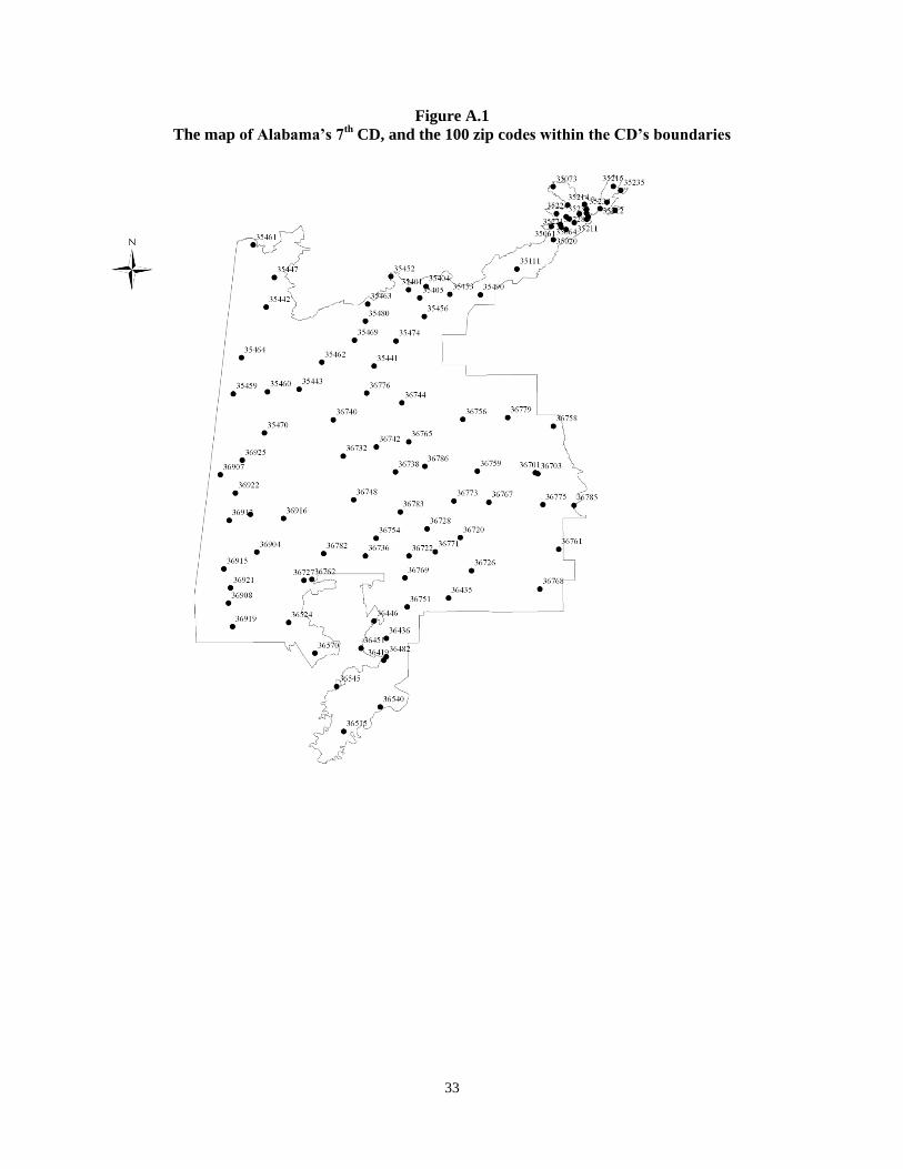
33

Figure A.1

The map of Alabama’s 7th

CD, and the 100 zip codes within the CD’s boundaries

34

Appendix B

Table B.1 below lists the Senate and House committees and their industry jurisdictions. Industry

jurisdictions are from the Congressional committees’ websites and are supplemented with data on

committee jurisdiction from the Center for Responsive Politics. We first match the jurisdiction data with

the Fama-French 48 industry definitions and then verify and supplement the matching with 4-digit SIC

code definitions.

Table B.1

Congressional committee jurisdictions

Senate committee FF-48 industry Additional industries defined at the SIC 4-digit level

Agriculture, Nutrition,

and Forestry

Agriculture

Food

Smoke

0800 – 0899 (Forestry)

5143, 5450, 5451 & 2020 (Dairy products and stores)

5144, 2015 (Poultry and eggs)

6220 – 6221 (Commodity brokers & dealers)

Armed Services Guns 3721, 3720, 3724, 3728 (Aircraft, engine and parts)

Banking, Housing,

and Urban Affairs

Banks

Construction

Health

Insurance

Real estate

Trading

Commerce, Science,

and Transportation

Aero

Autos

Fun

Insurance

Meals

Oil

Telecomm

Transportation

4520, 4522, 4512 (Air transport)

5146, 0920, 0921, 0900, 0910 (Commercial fishing and

wholesale)

3740, 3743 (Railroad equipment)

3730 – 3731 (Ship building and repair)

7510, 7515 (Auto and truck rental)

Energy and Natural

Resources

Mines

Oil

Utilities

0800 – 0899 (Forestry)

5093 (Scrap and waste materials)

Environment and

Public Works

Autos

Building materials

Chemicals

Construction

Mines

Oil

Utilities

5146, 0920, 0921, 0900, 0910 (Commercial fishing and

wholesale)

1520, 1540, 1541, 1521, 1542, 1522 (General contractors)

7510, 7515 (Auto and truck rental)

5093 (Scrap and waste materials)

35

Table B.1 - continued

House committee FF 48- industry Additional industries defined at the SIC 4-digit level

Agriculture

Agriculture

Food

Smoke

0800 – 0899 (Forestry)

5143, 5450, 5451 & 2020 (Dairy products and stores)

5144, 2015 (Poultry and eggs)

6220 – 6221 (Commodity brokers & dealers)

Armed

Services/National

Security

Guns 3721, 3720, 3724, 3728 (Aircraft, engine and parts)

Financial Services

Banks

Construction

Health

Insurance

Real estate

Trading

Energy and

Commerce

Autos

Chemicals

Utilities

Health

Meals

Mines

Oil

Drugs

Medical equipment

Fun

Telecomm

5093 (Scrap and waste materials)

Resources/Natural

Resources

Mines

Oil

5146, 0920, 0921, 0900, 0910 (Commercial fishing and

wholesale)

0800 – 0899 (Forestry)

Transportation and

Infrastructure

Aero

Autos

Construction

Building materials

Transportation

4520, 4522, 4512 (Air transport)

1520, 1540, 1541, 1521, 1542, 1522 (General contractors)

3740, 3743 (Railroad equipment)

3730 – 3731 (Ship building and repair)

7510, 7515 (Auto and truck rental)

Merchant Marine and

Fisheries

5146, 0920, 0921, 0900, 0910 (Commercial fishing and

wholesale)

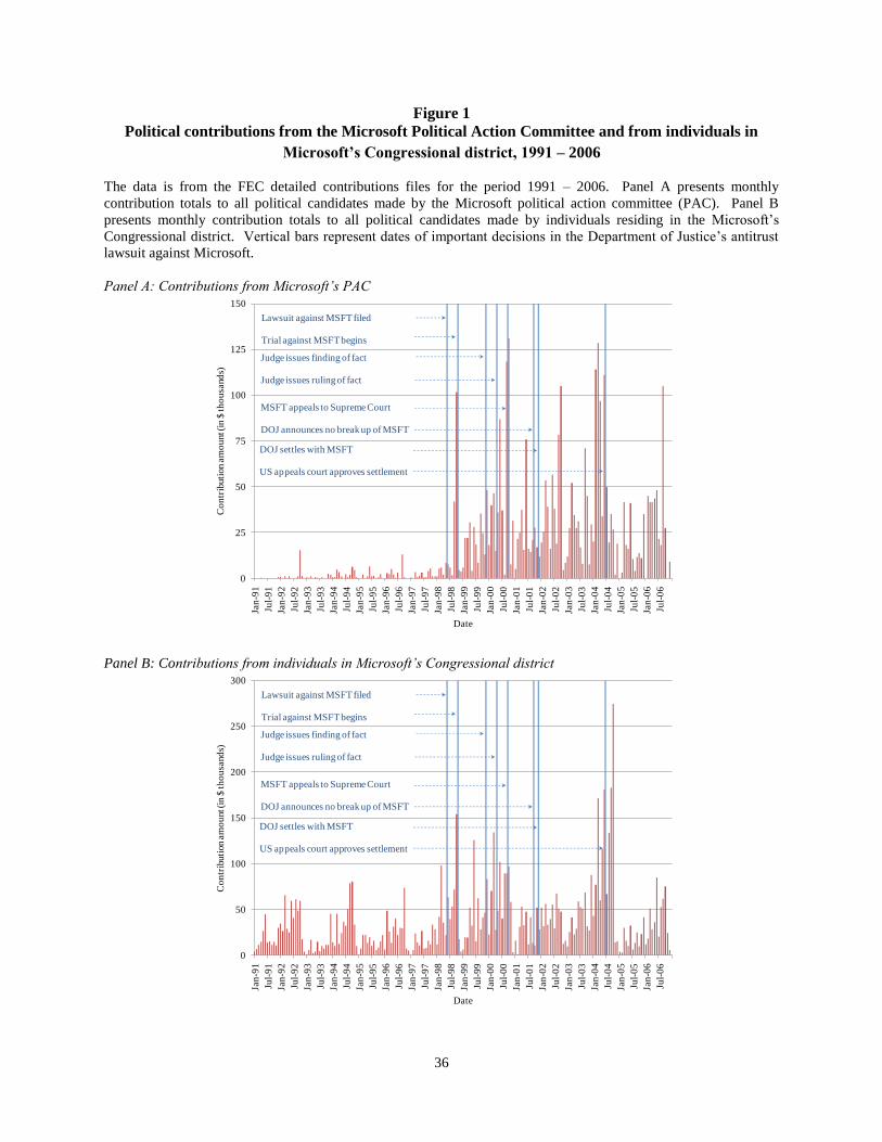
36

Figure 1

Political contributions from the Microsoft Political Action Committee and from individuals in

Microsoft’s Congressional district, 1991 – 2006

The data is from the FEC detailed contributions files for the period 1991 – 2006. Panel A presents monthly

contribution totals to all political candidates made by the Microsoft political action committee (PAC). Panel B

presents monthly contribution totals to all political candidates made by individuals residing in the Microsoft’s

Congressional district. Vertical bars represent dates of important decisions in the Department of Justice’s antitrust

lawsuit against Microsoft.

Panel A: Contributions from Microsoft’s PAC

Panel B: Contributions from individuals in Microsoft’s Congressional district

0

25

50

75

100

125

150

Jan

-91

Jul-

91

Jan

-92

Jul-

92

Jan

-93

Jul-

93

Jan

-94

Jul-

94

Jan

-95

Jul-

95

Jan

-96

Jul-

96

Jan

-97

Jul-

97

Jan

-98

Jul-

98

Jan

-99

Jul-

99

Jan

-00

Jul-

00

Jan

-01

Jul-

01

Jan

-02

Jul-

02

Jan

-03

Jul-

03

Jan

-04

Jul-

04

Jan

-05

Jul-

05

Jan

-06

Jul-

06

Co

ntr

ibuti

on a

mo

unt (

in $

th

ou

sand

s)

Date

Lawsuit against MSFT filed

Trial against MSFT begins

Judge issues finding of fact

Judge issues ruling of fact

MSFT appeals to Supreme Court

DOJ announces no break up of MSFT

DOJ settles with MSFT

US appeals court approves settlement

0

50

100

150

200

250

300

Jan

-91

Jul-

91

Jan

-92

Jul-

92

Jan

-93

Jul-

93

Jan

-94

Jul-

94

Jan

-95

Jul-

95

Jan

-96

Jul-

96

Jan

-97

Jul-

97

Jan

-98

Jul-

98

Jan

-99

Jul-

99

Jan

-00

Jul-

00

Jan

-01

Jul-

01

Jan

-02

Jul-

02

Jan

-03

Jul-

03

Jan

-04

Jul-

04

Jan

-05

Jul-

05

Jan

-06

Jul-

06

Co

ntr

ibuti

on a

mo

unt (

in $

th

ou

sand

s)

Date

Lawsuit against MSFT filed

Trial against MSFT begins

Judge issues finding of fact

Judge issues ruling of fact

MSFT appeals to Supreme Court

DOJ announces no break up of MSFT

DOJ settles with MSFT

US appeals court approves settlement

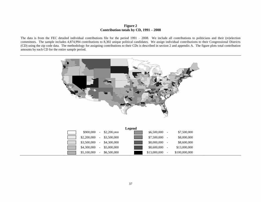
37

Figure 2

Contribution totals by CD, 1991 – 2008

The data is from the FEC detailed individual contributions file for the period 1991 – 2008. We include all contributions to politicians and their (re)election

committees. The sample includes 4,874,994 contributions to 8,302 unique political candidates. We assign individual contributions to their Congressional Districts

(CD) using the zip code data. The methodology for assigning contributions to their CDs is described in section 2 and appendix A. The figure plots total contribution

amounts by each CD for the entire sample period.

$900,000 - $2,200,000

$2,200,000 - $3,500,000

$3,500,000 - $4,300,000

$4,300,000 - $5,000,000

$5,100,000 - $6,500,000

$6,500,000 - $7,500,000

$7,500,000 - $8,000,000

$8,000,000 - $8,600,000

$8,600,000 - $13,000,000

$13,000,000 - $100,000,000

Legend

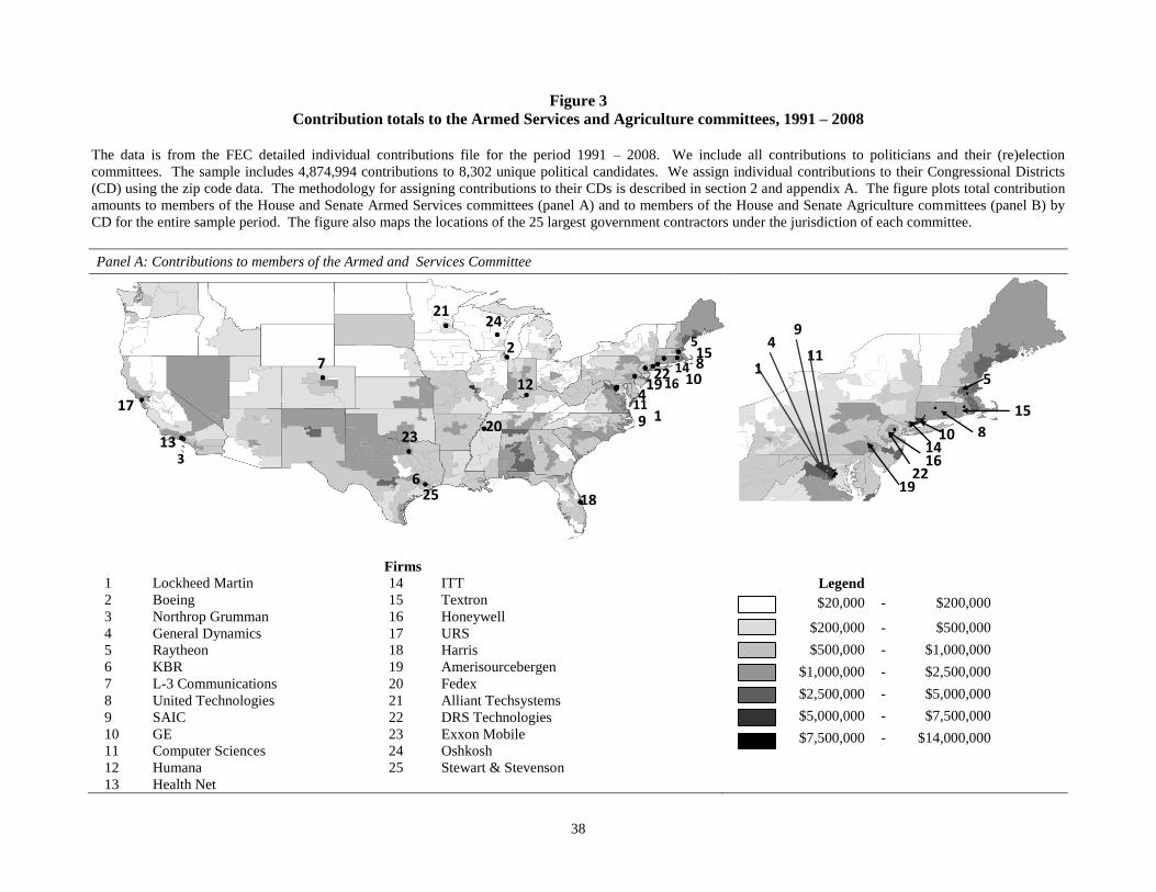
38

Figure 3

Contribution totals to the Armed Services and Agriculture committees, 1991 – 2008

The data is from the FEC detailed individual contributions file for the period 1991 – 2008. We include all contributions to politicians and their (re)election

committees. The sample includes 4,874,994 contributions to 8,302 unique political candidates. We assign individual contributions to their Congressional Districts

(CD) using the zip code data. The methodology for assigning contributions to their CDs is described in section 2 and appendix A. The figure plots total contribution

amounts to members of the House and Senate Armed Services committees (panel A) and to members of the House and Senate Agriculture committees (panel B) by

CD for the entire sample period. The figure also maps the locations of the 25 largest government contractors under the jurisdiction of each committee.

Panel A: Contributions to members of the Armed and Services Committee

Firms

1 Lockheed Martin 14 ITT

2 Boeing 15 Textron

3 Northrop Grumman 16 Honeywell

4 General Dynamics 17 URS

5 Raytheon 18 Harris

6 KBR 19 Amerisourcebergen

7 L-3 Communications 20 Fedex

8 United Technologies 21 Alliant Techsystems

9 SAIC 22 DRS Technologies

10 GE 23 Exxon Mobile

11 Computer Sciences 24 Oshkosh

12 Humana 25 Stewart & Stevenson

13 Health Net

Legend

$20,000 - $200,000

$200,000 - $500,000

$500,000 - $1,000,000

$1,000,000 - $2,500,000

$2,500,000 - $5,000,000

$5,000,000 - $7,500,000

$7,500,000 - $14,000,000

5

15

14 10

16 22

19

11 4

1

9

8

5 15

14 10 16

22 19

11 4

1 9

8

17

13

25

3

23

6

18

20

12

21 24

2 7

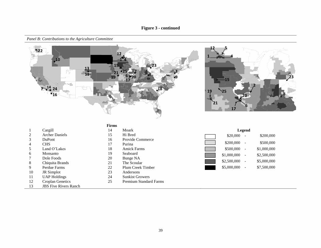
39

Figure 3 - continued

Panel B: Contributions to the Agriculture Committee

Firms

1 Cargill 14 Moark

2 Archer Daniels 15 Hi Bred

3 DuPont 16 Provide Commerce

4 CHS 17 Purina

5 Land O’Lakes 18 Amick Farms

6 Monsanto 19 Seaboard

7 Dole Foods 20 Bunge NA

8 Chiquita Brands 21 The Scoular

9 Perdue Farms 22 Plum Creek Timber

10 JR Simplot 23 Andersons

11 UAP Holdings 24 Sunkist Growers

12 Croplan Genetics 25 Premium Standard Farms

13 JBS Five Rivers Ranch

Legend

$20,000 - $200,000

$200,000 - $500,000

$500,000 - $1,000,000

$1,000,000 - $2,500,000

$2,500,000 - $5,000,000

$5,000,000 - $7,500,000

5

15

20

21

17

25 19

12

4 1

6

15

14

16

23

18

3

4

17 9

8

22

10 5

11 19 6

2

20

12

25

24

1

13

7

21

2

8

23

40

Figure 4

T-statistics from tobit regressions by state, 1991 – 2008

The data is from the FEC detailed individual contributions file for the period 1991 – 2008. We include all contributions to politicians and their (re)election

committees. The sample includes 4,874,994 contributions to 8,302 unique political candidates. We assign individual contributions to their Congressional Districts

(CD) using the zip code data. The methodology for assigning contributions to their CDs is described in section 2 and appendix A. The figure plots t-statistics from

state-by-state tobit regressions of the amount of political contributions from each CD on EDDFirms

. EDDFirms

is defined in equation 2 in section 2 and measures the

total number of firms in each CD that operate under the jurisdiction of a given politician. The vertical bars represent the total number of Fortune 500 firms located

in each state.

Legend

No data

< 0

0.00 - 1.00

1.00 - 2.00

2.00 - 5.00

> 5.00

41

Table 1

Congressional district contribution characteristics, 1991 - 2008

The data is from the FEC detailed individual contributions file for the period 1991 – 2008. We include all contributions to politicians and their (re)election

committees. The sample includes 4,874,994 contributions to 8,302 unique political candidates. We assign individual contributions to their Congressional Districts

(CD) using the zip code data. The methodology for assigning contributions to their CDs is described in section 2 and appendix A. The table reports CD

contribution characteristics per CD per election cycle. All contribution amounts in the left side of the table are in 12/2008 dollars.

Amount of contributions per election cycle

Number of supported candidates per election cycle

Variable Mean Min 25th Per Median 75th Per Max

Mean Min 25th Per Median 75th Per Max

Total contributions $875,356 4,573 300,657 528,640 969,925 19,610,903 104 4 52 79 125 883

Candidates

Democrats 433,242 6,981 101,936 213,470 453,719 13,731,011 52 1 22 38 63 491

Republicans 435,047 4,204 142,518 280,456 519,753 8,411,722 49 1 26 38 59 414

Races

House 412,473 1,786 150,730 274,388 496,191 6,341,969 65 1 30 46 75 690

Senate 390,084 1,363 82,439 183,900 413,555 12,723,660 34 1 17 28 44 174

Congressional committees

Appropriations 63,541 197 5,335 17,841 57,186 1,929,710 6 1 3 4 8 26

Small Business 54,445 197 4,289 13,561 48,057 2,070,840 5 0 2 4 6 18

Armed Services 54,201 911 4,023 13,706 50,499 3,300,991 5 0 2 4 6 21

Banking 54,047 552 3,575 12,502 44,944 3,406,934 4 0 2 3 6 19

Judiciary 53,765 142 3,422 11,944 42,188 3,646,303 4 0 2 3 5 17

Commerce 48,984 117 3,976 12,082 40,419 2,084,462 5 1 2 4 6 21

Foreign Relations 48,541 259 3,472 11,019 40,020 1,431,820 4 0 2 3 6 19

Budget 47,307 361 3,740 12,420 40,941 2,042,063 4 0 2 4 6 21

Environment 45,815 371 2,910 9,706 33,884 2,854,661 4 1 2 3 5 18

Labor 42,474 142 3,311 10,179 33,278 2,379,084 4 0 2 3 5 19

42

Table 2

EDD variables descriptive statistics, 1991 – 2008

The data is from the FEC detailed individual contributions file for the period 1991 – 2008. We include all contributions to

politicians and their (re)election committees. The sample includes 4,874,994 contributions to 8,302 unique political

candidates. We assign individual contributions to their Congressional Districts (CD) using the zip code data. The

methodology for assigning contributions to their CDs is described in section 2 and appendix A. The table presents the

descriptive statistics for the economic dependence variables used in the paper. The economic dependence variables are

defined in equations 1 – 4 in section 2. Panel A describes the economic dependence variables. Panel B summarizes the total

amount of contributions per year made by economically dependent CDs and non-economically dependent CDs to each

politician in our sample.

Variable Mean Min 25th Per Median 75th Per Max

Panel A: Characteristics of economically dependent CDs

Percent economically relevant politicians (%) 23.99 0 14.29 24.81 33.33 81.25

Number of economically dependent firms 3.74 1 1.50 2.60 4.41 55.63

Assets of economically dependent firms ($ billions) 3.103 0.002 0.378 0.985 2.957 255.448

Employees of economically dependent firms (thousands) 3.997 0.110 0.307 1.256 3.735 218.286

Panel B: Contribution totals from economically dependent and non-dependent CDs

Percent financing raised from economically dependent CDs (%) 18.61 0 0 0 18.75 100.00

Contributions from EDD districts 195.71 1 18 73 196 100,017

Contributions from non-EDD districts 166.67 1 6 32 138 94,854

Amount raised from EDD districts ($) 157,787 255 12,904 23,103 147,409 9,177,554

Amount raised from non-EDD districts ($) 125,136 133 4,207 53,387 99,929 5,110,662

43

Table 3

Political contributions from economically dependent Congressional districts, 1991 – 2008

The data is from the FEC detailed individual contributions file for the period 1991 – 2008. We include all

contributions to politicians and their (re)election committees. The sample includes 4,874,994 contributions to 8,302

unique political candidates. We assign individual contributions to their Congressional Districts (CD) using the zip

code data. The methodology for assigning contributions to their CDs is described in section 2 and appendix A. For

each CD, we compute four measures of its economic dependence. The economic dependence variables are

described in equations 1 – 4 in section 2. The table estimates 12 regressions that relate the CD contribution intensity

to its economic dependence status. The regression specification in panel A is described in equation 5 in section 3.

The regression specification in panel B is described in equation 7 in equation 3. All regressions are estimated with

CD and politician fixed effects. Each regression includes 624,071 observations from CDs and politicians with a

non-zero within-CD and within-politician variation in the independent variables. Columns 2 and 3 present the

results from the logit model that relates the contribution probability to the CD economic dependence status.

Columns 4 and 5 present the results from the poisson model that relates the contribution frequency to the CD

economic dependence status. Columns 6 and 7 present the results from the tobit model that relates the contribution

total amount to the CD economic dependence status. We estimate each model for every year of data and then

average the coefficients across years and compute standard errors from the time-series variation in parameter

estimates. Standard errors (SE) are reported in parentheses. a,

b,

c, indicates significance at the 1%, 5%, and 10%

level, respectively.

Logit Poisson Tobit

Variable Parameter SE Parameter SE Parameter SE

Panel A: Main results

EDD 0.0322 c (0.0159) 0.1004 a (0.0259) 230.47 c (113.54)

EDDFirms 0.0075 a (0.0009) 0.0104 a (0.0021) 104.60 a (16.66)

EDDAssets 0.0004 a (0.0001) 0.0011 a (0.0003) 10.11 a (2.57)

EDDEmployees 0.0005 a (0.0002) 0.0004 (0.0003) 6.36 a (1.60)

Panel B: Interactions with politician’s own district indicator

EDD 0.0147 (0.0159) 0.0154 (0.0197) 57.65 (122.91)

EDD × OD 0.1677 c (0.0885) -0.0567 (0.0405) 1,761.98 (2,020.86)

EDDFirms 0.0072 a (0.0010) 0.0077 a (0.0012) 75.20 a (12.70)

EDDFirms × OD 0.0501 a (0.0140) -0.0107 b (0.0045) 803.87 b (319.49)

EDDAssets 0.0004 a (0.0001) 0.0009 a (0.0003) 6.50 a (1.56)

EDDAssets × OD 0.0085 b (0.0030) -0.0012 a (0.0004) 101.04 b (38.57)

EDDEmployees 0.0004 b (0.0002) 0.0006 b (0.0003) 3.36 b (1.17)

EDDEmployees × OD 0.0066 b (0.0024) -0.0015 b (0.0005) 59.23 b (23.74)

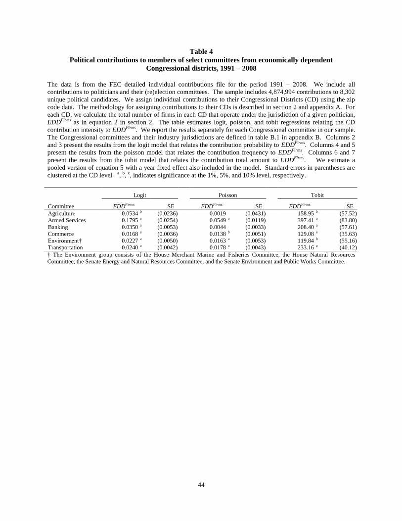
44

Table 4

Political contributions to members of select committees from economically dependent

Congressional districts, 1991 – 2008

The data is from the FEC detailed individual contributions file for the period 1991 – 2008. We include all

contributions to politicians and their (re)election committees. The sample includes 4,874,994 contributions to 8,302

unique political candidates. We assign individual contributions to their Congressional Districts (CD) using the zip

code data. The methodology for assigning contributions to their CDs is described in section 2 and appendix A. For

each CD, we calculate the total number of firms in each CD that operate under the jurisdiction of a given politician,

EDDFirms

as in equation 2 in section 2. The table estimates logit, poisson, and tobit regressions relating the CD

contribution intensity to EDDFirms

. We report the results separately for each Congressional committee in our sample.

The Congressional committees and their industry jurisdictions are defined in table B.1 in appendix B. Columns 2

and 3 present the results from the logit model that relates the contribution probability to EDDFirms

. Columns 4 and 5

present the results from the poisson model that relates the contribution frequency to EDDFirms

. Columns 6 and 7

present the results from the tobit model that relates the contribution total amount to EDDFirms

. We estimate a

pooled version of equation 5 with a year fixed effect also included in the model. Standard errors in parentheses are

clustered at the CD level. a,

b,

c, indicates significance at the 1%, 5%, and 10% level, respectively.

Logit Poisson Tobit

Committee EDDFirms SE EDDFirms SE EDDFirms SE

Agriculture 0.0534 b (0.0236) 0.0019 (0.0431) 158.95 b (57.52)

Armed Services 0.1795 a (0.0254) 0.0549 a (0.0119) 397.41 a (83.80)

Banking 0.0350 a (0.0053) 0.0044 (0.0033) 208.40 a (57.61)

Commerce 0.0168 a (0.0036) 0.0138 b (0.0051) 129.08 a (35.63)

Environment† 0.0227 a (0.0050) 0.0163 a (0.0053) 119.84 b (55.16)

Transportation 0.0240 a (0.0042) 0.0178 a (0.0043) 233.16 a (40.12)

† The Environment group consists of the House Merchant Marine and Fisheries Committee, the House Natural Resources

Committee, the Senate Energy and Natural Resources Committee, and the Senate Environment and Public Works Committee.

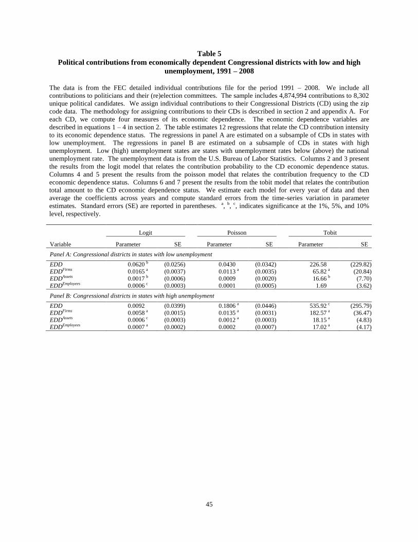
45

Table 5

Political contributions from economically dependent Congressional districts with low and high

unemployment, 1991 – 2008

The data is from the FEC detailed individual contributions file for the period 1991 – 2008. We include all

contributions to politicians and their (re)election committees. The sample includes 4,874,994 contributions to 8,302

unique political candidates. We assign individual contributions to their Congressional Districts (CD) using the zip

code data. The methodology for assigning contributions to their CDs is described in section 2 and appendix A. For

each CD, we compute four measures of its economic dependence. The economic dependence variables are

described in equations 1 – 4 in section 2. The table estimates 12 regressions that relate the CD contribution intensity

to its economic dependence status. The regressions in panel A are estimated on a subsample of CDs in states with

low unemployment. The regressions in panel B are estimated on a subsample of CDs in states with high

unemployment. Low (high) unemployment states are states with unemployment rates below (above) the national

unemployment rate. The unemployment data is from the U.S. Bureau of Labor Statistics. Columns 2 and 3 present

the results from the logit model that relates the contribution probability to the CD economic dependence status.

Columns 4 and 5 present the results from the poisson model that relates the contribution frequency to the CD

economic dependence status. Columns 6 and 7 present the results from the tobit model that relates the contribution

total amount to the CD economic dependence status. We estimate each model for every year of data and then

average the coefficients across years and compute standard errors from the time-series variation in parameter

estimates. Standard errors (SE) are reported in parentheses. a,

b,

c, indicates significance at the 1%, 5%, and 10%

level, respectively.

Logit Poisson Tobit

Variable Parameter SE Parameter SE Parameter SE

Panel A: Congressional districts in states with low unemployment

EDD 0.0620 b (0.0256) 0.0430 (0.0342) 226.58 (229.82)

EDDFirms 0.0165 a (0.0037) 0.0113 a (0.0035) 65.82 a (20.84)

EDDAssets 0.0017 b (0.0006) 0.0009 (0.0020) 16.66 b (7.70)

EDDEmployees 0.0006 c (0.0003) 0.0001 (0.0005) 1.69 (3.62)

Panel B: Congressional districts in states with high unemployment

EDD 0.0092 (0.0399) 0.1806 a (0.0446) 535.92 c (295.79)

EDDFirms 0.0058 a (0.0015) 0.0135 a (0.0031) 182.57 a (36.47)

EDDAssets 0.0006 c (0.0003) 0.0012 a (0.0003) 18.15 a (4.83)

EDDEmployees 0.0007 a (0.0002) 0.0002 (0.0007) 17.02 a (4.17)

46

Table 6

Firm operating performance as a function of individual political contributions, 1991 – 2008

The political contributions data is from the FEC detailed individual contributions file for the period 1991 – 2008. We include all contributions to politicians and their

(re)election committees. The sample includes 4,874,994 contributions to 8,302 unique political candidates. We calculate two measures of contribution intensity. The

first measure, EDDCit-1, is the frequency and the amount of contributions made by individuals in firm i’s Congressional district to economically relevant politicians, i.e.

politicians who serve on Congressional committees with jurisdiction over firm i’s industry. The second measure, Cit-1, is the frequency and the amount of contributions

made by individuals in firm i’s Congressional district to all other politicians. We merge our contributions variable with Compustat. The merged sample is 99,501 firm-

years for the period 1991 – 2008. We then regress industry-adjusted ROA and market-to-book changes on the political contributions measures and other control variables.

All variables are defined in section 4. Panel A presents the results for the ROA regressions. Panel B presents the results for the market-to-book regressions. Standard

errors are adjusted for heteroskedasticity and clustered by firm and year and are reported in parentheses. a,

b,

c, indicates significance at the 1%, 5%, and 10% level,

respectively.

Frequency of contributions

Amount of contributions

Variable Parameter

SE Parameter

SE Parameter

SE

Parameter

SE Parameter

SE Parameter

SE

Panel A: ROA analysis

Intercept -0.0024 (0.0022) -0.0023 (0.0022) -0.0023 (0.0022) -0.0024 (0.0022) -0.0023 (0.0022) -0.0023 (0.0022)

Ln(Q) 0.0027 (0.0021) 0.0030 (0.0021) 0.0029 (0.0020) 0.0027 (0.0021) 0.0030 (0.0021) 0.0029 (0.0021)

Ln(Size) -0.0041 b (0.0019) -0.0045 b (0.0019) -0.0045 b (0.0019) -0.0041 b (0.0019) -0.0045 b (0.0019) -0.0045 b (0.0019)

∆ ROA -0.0454 a (0.0114) -0.0454 a (0.0114) -0.0454 a (0.0114) -0.0454 a (0.0114) -0.0454 a (0.0114) -0.0454 a (0.0114)

Ln(CFrequency) 0.0021 (0.0014) 0.0016 (0.0015)

Ln(EDDCFrequency) 0.0029 a (0.0005) 0.0026 a (0.0007)

Ln(CAmount) 0.0018 c (0.0010) 0.0012 (0.0011)

Ln(EDDCAmount) 0.0033 a (0.0007) 0.0031 a (0.0008)

Panel B: Market-to-book analysis

Intercept -0.0859 a (0.0270) -0.0839 a (0.0260) -0.0837 a (0.0258) -0.0860 a (0.0271) -0.0833 a (0.0257) -0.0831 a (0.0257)

CAPX -0.1136 a (0.0337) -0.1266 a (0.0379) -0.1271 a (0.0380) -0.1137 a (0.0337) -0.1266 a (0.0380) -0.1267 a (0.0380)

RD / A -0.1171 b (0.0471) -0.1112 b (0.0450) -0.1105 b (0.0448) -0.1172 b (0.0472) -0.1125 b (0.0454) -0.1123 b (0.0454)

Ln(Size) -0.1703 a (0.0630) -0.1786 a (0.0651) -0.1781 a (0.0649) -0.1706 a (0.0632) -0.1791 a (0.0653) -0.1788 a (0.0652)

ROA 0.0310 (0.0880) 0.0390 (0.0898) 0.0381 (0.0894) 0.0314 (0.0881) 0.0395 (0.0899) 0.0391 (0.0898)

Ln(CFrequency) -0.0035 (0.0070) -0.0198 c (0.0107)

Ln(EDDCFrequency) 0.0770 a (0.0289) 0.0811 a (0.0305)

Ln(CAmount) 0.0037 (0.0050) -0.0114 c (0.0067)

Ln(EDDCAmount) 0.0812 a (0.0313) 0.0832 a (0.0321)

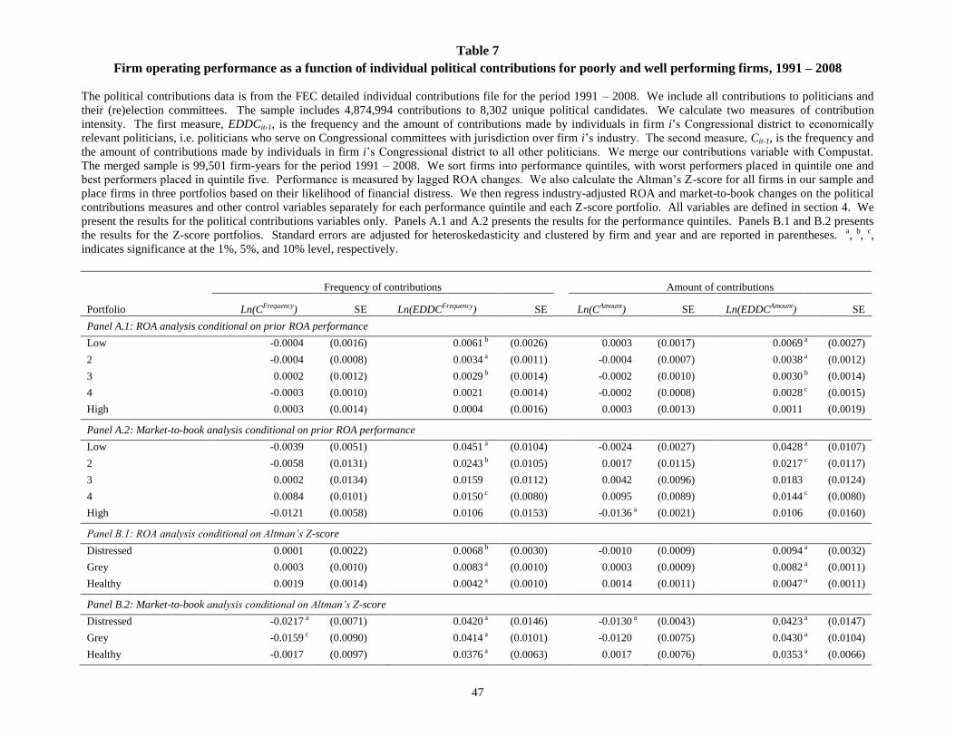
47

Table 7

Firm operating performance as a function of individual political contributions for poorly and well performing firms, 1991 – 2008

The political contributions data is from the FEC detailed individual contributions file for the period 1991 – 2008. We include all contributions to politicians and

their (re)election committees. The sample includes 4,874,994 contributions to 8,302 unique political candidates. We calculate two measures of contribution

intensity. The first measure, EDDCit-1, is the frequency and the amount of contributions made by individuals in firm i’s Congressional district to economically

relevant politicians, i.e. politicians who serve on Congressional committees with jurisdiction over firm i’s industry. The second measure, Cit-1, is the frequency and

the amount of contributions made by individuals in firm i’s Congressional district to all other politicians. We merge our contributions variable with Compustat.

The merged sample is 99,501 firm-years for the period 1991 – 2008. We sort firms into performance quintiles, with worst performers placed in quintile one and

best performers placed in quintile five. Performance is measured by lagged ROA changes. We also calculate the Altman’s Z-score for all firms in our sample and

place firms in three portfolios based on their likelihood of financial distress. We then regress industry-adjusted ROA and market-to-book changes on the political

contributions measures and other control variables separately for each performance quintile and each Z-score portfolio. All variables are defined in section 4. We

present the results for the political contributions variables only. Panels A.1 and A.2 presents the results for the performance quintiles. Panels B.1 and B.2 presents

the results for the Z-score portfolios. Standard errors are adjusted for heteroskedasticity and clustered by firm and year and are reported in parentheses. a,

b,

c,

indicates significance at the 1%, 5%, and 10% level, respectively.

Frequency of contributions Amount of contributions

Portfolio Ln(CFrequency)

SE Ln(EDDCFrequency)

SE Ln(CAmount)

SE Ln(EDDCAmount)

SE

Panel A.1: ROA analysis conditional on prior ROA performance

Low -0.0004 (0.0016) 0.0061 b (0.0026) 0.0003 (0.0017) 0.0069 a (0.0027)

2 -0.0004 (0.0008) 0.0034 a (0.0011) -0.0004 (0.0007) 0.0038 a (0.0012)

3 0.0002 (0.0012) 0.0029 b (0.0014) -0.0002 (0.0010) 0.0030 b (0.0014)

4 -0.0003 (0.0010) 0.0021 (0.0014) -0.0002 (0.0008) 0.0028 c (0.0015)

High 0.0003 (0.0014) 0.0004 (0.0016) 0.0003 (0.0013) 0.0011 (0.0019)

Panel A.2: Market-to-book analysis conditional on prior ROA performance

Low -0.0039 (0.0051) 0.0451 a (0.0104) -0.0024 (0.0027) 0.0428 a (0.0107)

2 -0.0058 (0.0131) 0.0243 b (0.0105) 0.0017 (0.0115) 0.0217 c (0.0117)

3 0.0002 (0.0134) 0.0159 (0.0112) 0.0042 (0.0096) 0.0183 (0.0124)

4 0.0084 (0.0101) 0.0150 c (0.0080) 0.0095 (0.0089) 0.0144 c (0.0080)

High -0.0121 (0.0058) 0.0106 (0.0153) -0.0136 a (0.0021) 0.0106 (0.0160)

Panel B.1: ROA analysis conditional on Altman’s Z-score

Distressed 0.0001 (0.0022) 0.0068 b (0.0030) -0.0010 (0.0009) 0.0094 a (0.0032)

Grey 0.0003 (0.0010) 0.0083 a (0.0010) 0.0003 (0.0009) 0.0082 a (0.0011)

Healthy 0.0019 (0.0014) 0.0042 a (0.0010) 0.0014 (0.0011) 0.0047 a (0.0011)

Panel B.2: Market-to-book analysis conditional on Altman’s Z-score

Distressed -0.0217 a (0.0071) 0.0420 a (0.0146) -0.0130 a (0.0043) 0.0423 a (0.0147)

Grey -0.0159 c (0.0090) 0.0414 a (0.0101) -0.0120 (0.0075) 0.0430 a (0.0104)

Healthy -0.0017 (0.0097) 0.0376 a (0.0063) 0.0017 (0.0076) 0.0353 a (0.0066)

48

Table 8

Firm operating performance as a function of individual political contributions in close elections and other elections, 1991 – 2008

The political contributions data is from the FEC detailed individual contributions file for the period 1991 – 2008. We include all contributions to politicians and their

(re)election committees. The sample includes 4,874,994 contributions to 8,302 unique political candidates. We calculate two measures of contribution intensity. The

first measure, EDDCit-1, is the frequency and the amount of contributions made by individuals in firm i’s Congressional district to economically relevant politicians, i.e.

politicians who serve on Congressional committees with jurisdiction over firm i’s industry. The second measure, Cit-1, is the frequency and the amount of contributions

made by individuals in firm i’s Congressional district to all other politicians. We merge our contributions variable with Compustat. The merged sample is 99,501 firm-

years for the period 1991 – 2008. We sort firms in quintiles based on the closeness of the economically relevant politician’s election outcome. Individuals in the firm’s

CD who contribute to economically relevant politicians in the closest elections are placed in quintile one and individuals in the firm’s CD who contribute to

economically relevant politicians in the elections with the biggest margin for victory are placed in quintile five. The regression is estimated only for those firm-years in

which individuals contribute positive amounts to economically relevant politicians, so the sample is reduced to 38,463 observations. We regress industry-adjusted ROA

and market-to-book changes on the political contributions measures and other control variables separately for each performance quintile. All variables are defined in

section 4. We present the results for the political contributions variables only. Panel A presents the results for the ROA regressions. Panel B presents the results for the

market-to-book regressions. Standard errors are adjusted for heteroskedasticity and clustered by firm and year and are reported in parentheses. a,

b,

c, indicates

significance at the 1%, 5%, and 10% level, respectively.

Frequency of contributions Amount of contributions

Portfolio Ln(CFrequency)

SE Ln(EDDCFrequency)

SE Ln(CAmount)

SE Ln(EDDCAmount)

SE

Panel A: ROA analysis

Contributions in close elections -0.0028 c (0.0015) 0.0034 a (0.0013) -0.0033 a (0.0012) 0.0037 b (0.0016)

Contributions in other elections 0.0012 (0.0009) -0.0012 (0.0010) 0.0011 (0.0008) -0.0009 (0.0010)

Panel B: Market-to-book analysis

Contributions in close elections -0.0006 (0.0108) 0.0217 b (0.0102) -0.0056 (0.0145) 0.0280 b (0.0134)

Contributions in other elections 0.0014 (0.0039) 0.0101 (0.0069) 0.0024 (0.0036) 0.0052 (0.0070)

49

Table 9

Changes in CD political contribution intensity around mergers, 1991 – 2008

The political contributions data is from the FEC detailed individual contributions file for the period 1991 – 2008. We

include all contributions to politicians and their (re)election committees. The original sample includes 4,874,994

contributions to 8,302 unique political candidates. We intersect this sample with a sample of mergers and

acquisitions for the period 1991 – 2008. The merger sample is from SDC and includes all public bidders and targets

that operate in different 4-digit SIC industries and in different Congressional districts (CDs). Further, we select

mergers in which the bidder owns less than 30 percent of the target prior to the merger and more than 50 percent of

the target after the merger and mergers in which the bidder’s and the target’s total assets in the year prior to the

merger are within 20 percent of each other. The table reports individual political contributions made from the bidder

and the target Congressional districts to the bidder’s and the target’s economically relevant politicians. Economic

relevant politicians are individuals who sit on Congressional committees with jurisdiction over the bidder’s or the

target’s industry. We calculate the average annual total number and total amount of contributions made to

economically relevant politicians during the pre- and post-merger periods. The pre-merger period is the period up to

12 months prior to the merger announcement. The post-merger period is the period at least 24 months after the

merger effective date. Panel A presents the results for the number of contributions during the pre- and post-merger

periods. Panel B presents the results for the amount of contributions during the pre- and post-merger periods. The

last column is the t-statistic from the t-test for the difference in mean contributions during the pre- and post-merger

periods.

Political contributions Variable label Pre-merger Post-merger difference t-statistic

Panel A: Contribution frequency

From bidder CD to bidder politicians BidEDDCBir 95.78 123.10 27.32 2.96

From bidder CD to target politicians BidEDDCTar 51.31 100.00 48.69 5.28

From target CD to bidder politicians TarEDDCBid 59.08 92.44 33.37 6.39

From target CD to target politicians TarEDDCTar 50.64 77.20 26.56 4.50

Panel B: Contribution amount (in $ thousands)

From bidder CD to bidder politicians BidEDDCBir 95.28 119.32 24.03 2.18

From bidder CD to target politicians BidEDDCTar 42.83 93.84 51.01 5.51

From target CD to bidder politicians TarEDDCBid 47.43 83.61 36.18 7.07

From target CD to target politicians TarEDDCTar 43.77 73.19 29.41 4.73

50

Table 10

Bidder firm operating performance as a function of individual political contributions received from the bidder and the target CDs, 1991 – 2008

The political contributions data is from the FEC detailed individual contributions file for the period 1991 – 2008. We include all contributions to politicians and their

(re)election committees. The sample includes 4,874,994 contributions to 8,302 unique political candidates. We calculate measures of the contribution intensity from the bidder

and the target Congressional districts to the bidder’s and the target’s economically relevant politicians. The contribution variables are described in table 9. We then regress

industry-adjusted ROA and market-to-book changes on the four political contributions measures and other control variables. All control variables are defined in section 4. Panel

A presents the results for the bidder ROA regressions. Panel B presents the results for the bidder market-to-book regressions. Standard errors are adjusted for heteroskedasticity

and clustered by firm and year and are reported in parentheses. a,

b,

c, indicates significance at the 1%, 5%, and 10% level, respectively.

Frequency of contributions

Amount of contributions

Variable Parameter

SE

Parameter

SE

Parameter

SE

Parameter

SE

Parameter

SE

Parameter

SE

Panel A: ROA analysis during the pre-merger period

Ln(BidEDDCBid) 0.0026 a (0.0009) 0.0024 a (0.0009) 0.0030 a (0.0011) 0.0028 a (0.0010)

Ln(BidEDDCTar) -0.0014 (0.0015) -0.0011 (0.0015)

Ln(TarEDDCBid) -0.0011 (0.0017) -0.0015 (0.0017)

Ln(TarEDDCTar) -0.0016 (0.0013) -0.0016 (0.0012) -0.0011 (0.0012) -0.0011 (0.0011)

Ln(BidEDDCBid)×Post -0.0004 (0.0015) -0.0003 (0.0012) -0.0008 (0.0013) -0.0008 (0.0013)

Ln(BidEDDCTar)×Post 0.0032 c (0.0018) 0.0027 (0.0019)

Ln(TarEDDCBid)×Post 0.0032 a (0.0011) 0.0035 a (0.0012)

Ln(TarEDDCTar)×Post 0.0036 c (0.0019) 0.0036 b (0.0018) 0.0033 c (0.0018) 0.0032 c (0.0018)

Panel B: Market-to-book analysis during the pre-merger period

Ln(BidEDDCBid) 0.0620 c (0.0320) 0.0582 c (0.0317) 0.0583 c (0.0350) 0.0530 (0.0354)

Ln(BidEDDCTar) -0.0245 (0.0269) -0.0227 (0.0276)

Ln(TarEDDCBid) 0.0233 (0.0286) 0.0296 (0.0326)

Ln(TarEDDCTar) 0.0016 (0.0290) -0.0000 (0.0292) 0.0056 (0.0306) 0.0066 (0.0312)

Ln(BidEDDCBid)×Post -0.0176 (0.0399) -0.0019 (0.0410) -0.0093 (0.0392) 0.0024 (0.0416)

Ln(BidEDDCTar)×Post 0.0545 c (0.0303) 0.0374 (0.0326)

Ln(TarEDDCBid)×Post 0.0211 (0.0487) 0.0485 (0.0492)

Ln(TarEDDCTar)×Post 0.0281 (0.0312) 0.0299 (0.0306) 0.0035 (0.0324) 0.0352 (0.0318)