Incremental Sampling Methodology (ISM)

• Part 1 - Introduction to ISM– Jeffrey E. Patterson– TCEQ, Technical Specialist, Superfund Section, Remediation Division– jeff.patterson@tceq.texas.gov – 512-239-2489– Member ITRC Committee on ISM

• Part 2 - ISM Field Implementation – Case Study– Ben Camacho– Daniel B. Stephens & Associates, Inc.– bcamacho@dbstephens.com– 512-651-6019

1

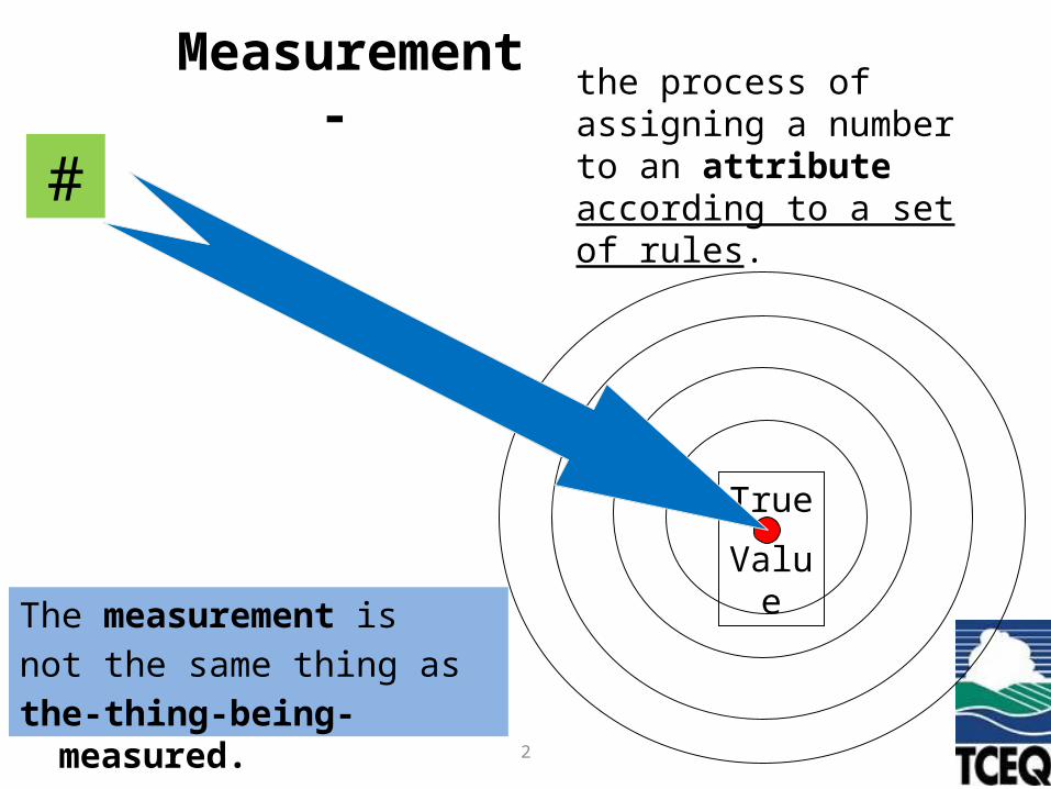
Measurement -

the process of assigning a number to an attribute according to a set of rules.

The measurement is not the same thing as the-thing-being-

measured. 2

True

Value

Measurement

#

Quote from EPA Guidance“Data users often look at a concentration obtained from a laboratory as being “THE CONCENTRATION” in the soil,

without realizing that the number generated by the laboratory is the end point of an entire process,

extending from design of the sampling, through collecting, handling, processing, analysis, quality evaluation, and reporting”.

(Soil Sampling Quality Assurance User’s Guide EPA/600/8-69/046)3

Volume to be Sampled

(e.g. 1/8th acre x 1 foot)

754,502,380 grams

DecisionWRONG

Decision?

RIGHT

Decision

?

Sample

226 grams

Field

Sampling

Sub-sampleLab

sub-sampling

30 grams300 ml

ExtractLab

Extraction

Assay Volume

10 uls

Extract

Sub-sampling

& Dilution

Analysis Result

Instrumental

Analysis

& Calculations

“..the end point of an entire process..”

A ratio of 25,000,000 to 1

4

Error associated with the sampling processes.

Most importantly

location of the sample!!

Measurement

True

Value

Mea

sure

men

t

Erro

rSa

mpl

ing

Erro

r

ErrorError associated with laboratory preparation &

analysis.

5

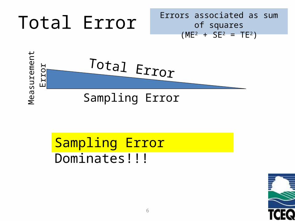
Total Error

Sampling Error Dominates!!!

6

Errors associated as sum of squares

(ME2 + SE2 = TE2)

Total Error

Measu

rem

en

t E

rror

Sampling Error

SOILS = PARTICULATE MATTER

• Natural soils are complex mixtures of: – different particle types, shapes, densities,

and – Particle sizes

• fine clays (4 µm diameter) to • coarse sand (2 mm in diameter).• 4 orders of magnitude.

• COC particle sizes in soil– fine airborne particles (<1 µm diameter)– to relatively large pellets.

7

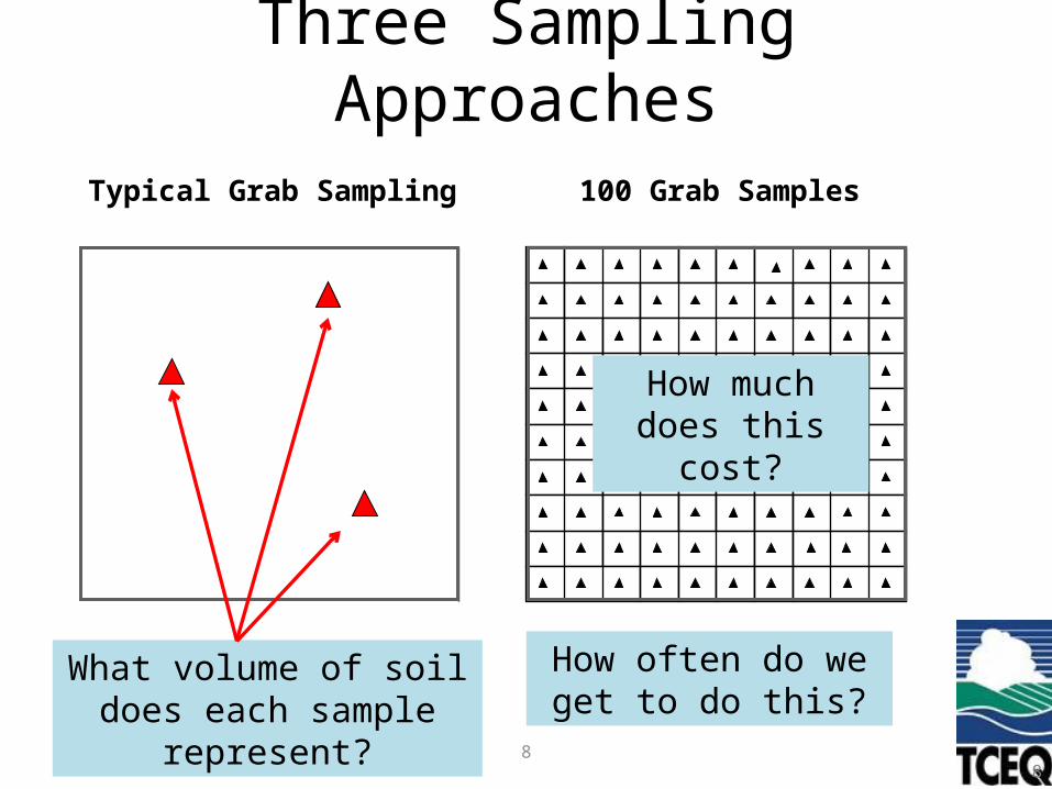
There are two types of grab sampling: Typically only a few discrete samples are collected from haphazardly selected locations – 3 grab samples are shown. In rare cases, many grab samples may be collected at regular intervals on a grid system – 100 samples are shown.

Three Sampling Approaches

8

Typical Grab Sampling

What volume of soil does each sample

represent?

100 Grab Samples

How often do we get to do this?

How much does this

cost?

8

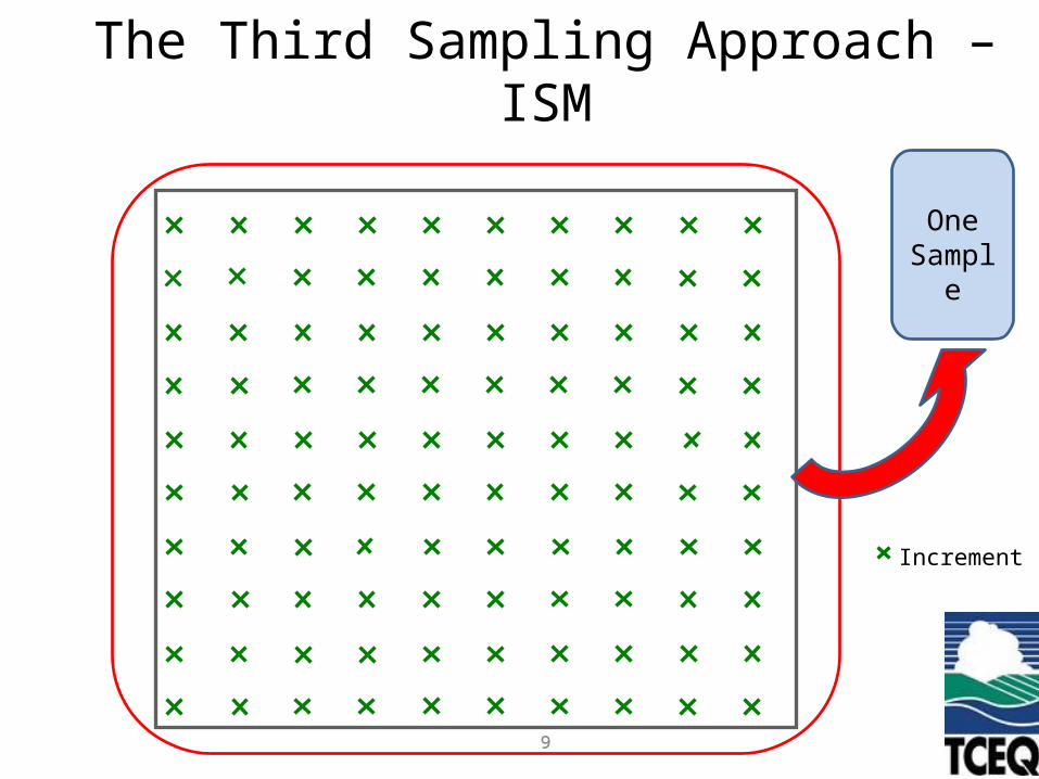
The third sampling approach is ISM sampling, where up to 100 increments are collected, combined and processed as a single sample.

99

The Third Sampling Approach – ISM

Increment

9

One Sampl

e

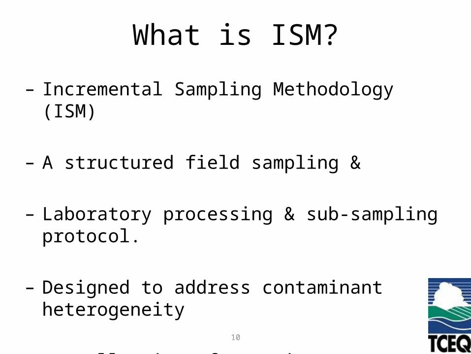
– Incremental Sampling Methodology (ISM)

– A structured field sampling &

– Laboratory processing & sub-sampling protocol.

– Designed to address contaminant heterogeneity

– By collection of many increments.

What is ISM?

10

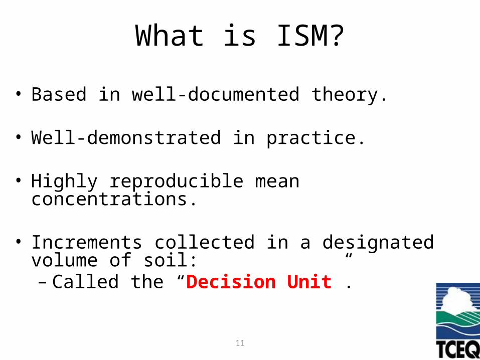
What is ISM?

• Based in well-documented theory.

• Well-demonstrated in practice.

• Highly reproducible mean concentrations.

• Increments collected in a designated volume of soil:– Called the “Decision Unit”.

11

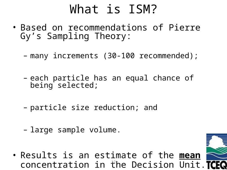
What is ISM?• Based on recommendations of Pierre Gy’s

Sampling Theory:

– many increments (30-100 recommended);

– each particle has an equal chance of being selected;

– particle size reduction; and

– large sample volume.

• Results is an estimate of the mean concentration in the Decision Unit.

12

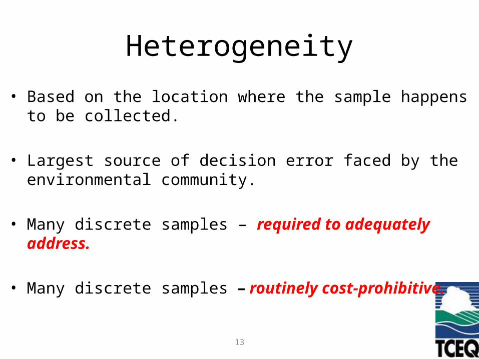
Heterogeneity

• Based on the location where the sample happens to be collected.

• Largest source of decision error faced by the environmental community.

• Many discrete samples – required to adequately address.

• Many discrete samples – routinely cost-prohibitive.

13

Heterogeneity Happens!• Large volumes of soil in the field ≠ test-tube

volumes.

• “Duplicate soil samples” do not produce duplicate results.

• Grab samples –

– huge variability

– over surprisingly small distances.

14

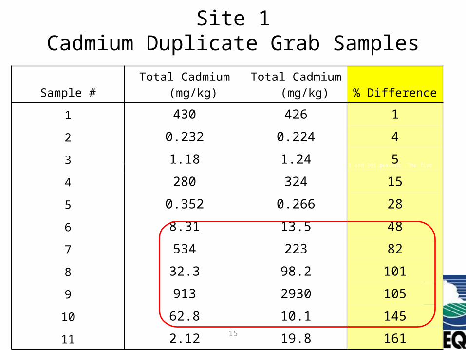
Sample #Total Cadmium

(mg/kg)Total Cadmium

(mg/kg) % Difference

1 430 426 1

2 0.232 0.224 4

3 1.18 1.24 5

4 280 324 15

5 0.352 0.266 28

6 8.31 13.5 48

7 534 223 82

8 32.3 98.2 101

9 913 2930 105

10 62.8 10.1 145

11 2.12 19.8 161

Site 1Cadmium Duplicate Grab Samples

• This table shows the percent difference between duplicate samples. The percent difference ranges between 1 and 161 percent. The five pairs of samples with the highest percent differences are highlighted with a box.

15

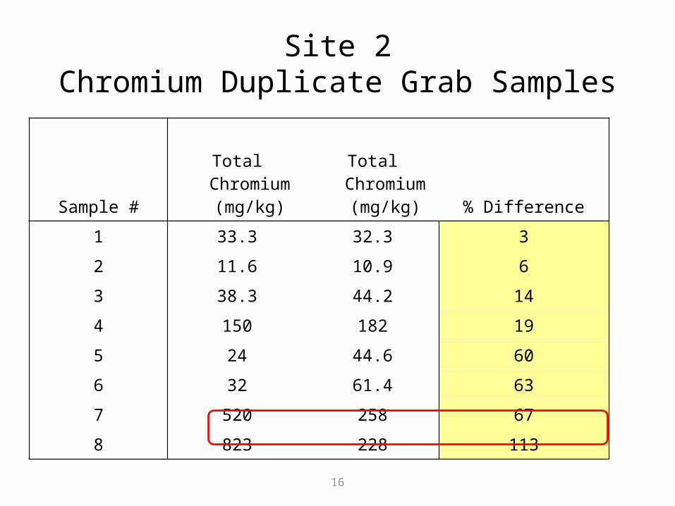
Site 2Chromium Duplicate Grab Samples

16

Sample #

Total Chromium (mg/kg)

Total Chromium (mg/kg) % Difference

1 33.3 32.3 3

2 11.6 10.9 6

3 38.3 44.2 14

4 150 182 19

5 24 44.6 60

6 32 61.4 63

7 520 258 67

8 823 228 113

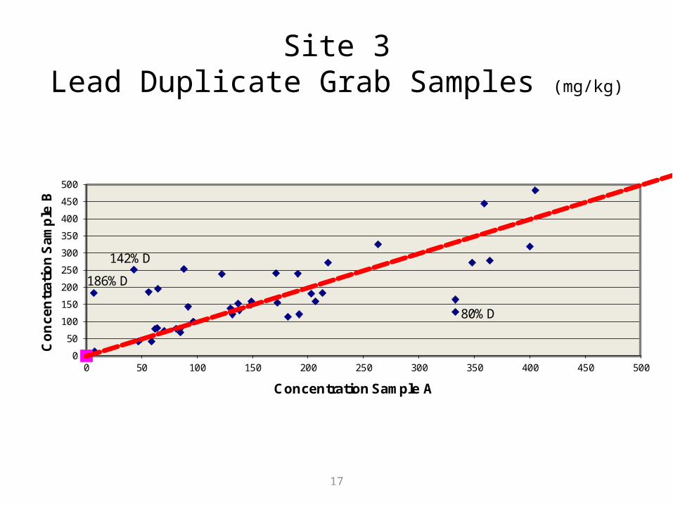
Site 3Lead Duplicate Grab Samples (mg/kg)

17

This point graph shows percent difference between duplicate samples.

The80%D

142%D

186%D

0

50

100

150

200

250

300

350

400

450

500

0 50 100 150 200 250 300 350 400 450 500

Co

nc

en

tra

tio

n S

am

ple

B

Concentration Sample A

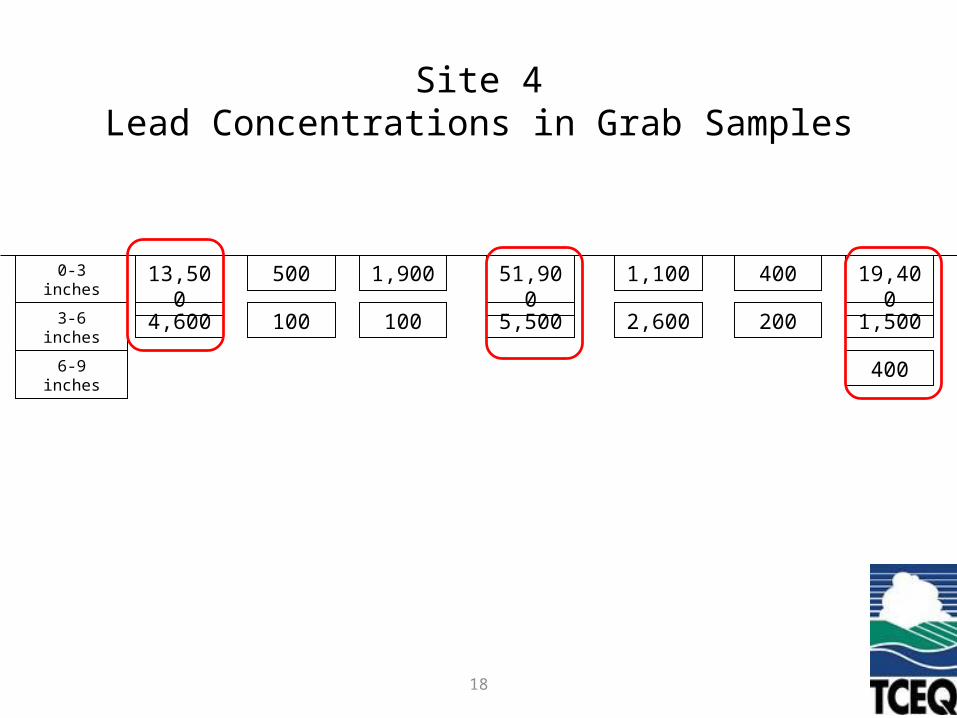
Site 4Lead Concentrations in Grab Samples

This schematic shows concentrations of grab samples collected in seven borings at various depth intervals: 0-3 inches, 3 to 6 inches and 6 to 9 inches deep.

18

13,500

4,600

1,900

100

51,900

5,500

1,100

2,600

400

200

19,400

1,5003-6 inches

400

500

100

0-3 inches

6-9 inches

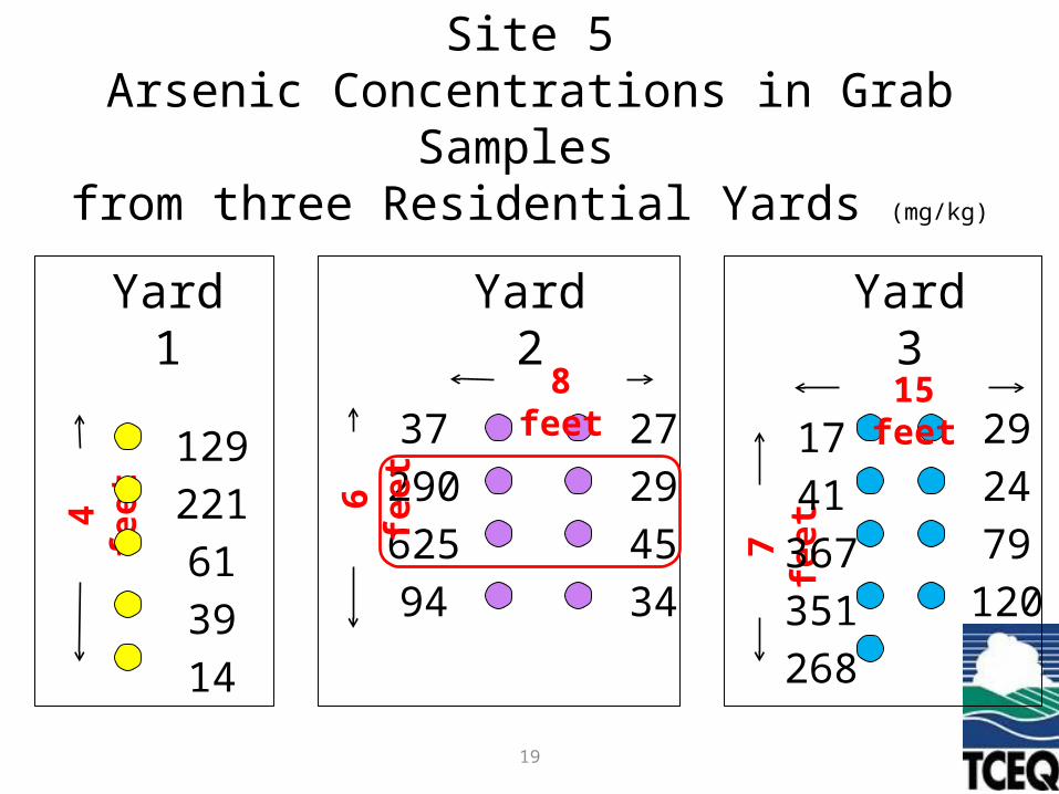
This schematic shows concentrations in grab samples collected within a few feet of each other in three different residential yards.

4

feet

Yard 1

Yard 2

Yard 3

129221613914

3729062594

27294534

6

feet

7 f

eet

8 feet

15 feet1741

367351268

292479

120

Site 5Arsenic Concentrations in Grab Samples

from three Residential Yards (mg/kg)

19

This schematic shows the concentrations of seven duplicate grab sample pairs located within 2 feet of each other in a circular pattern. The 2 pairs with the highest differences are highlighted with a box. Adapted from: “Sampling Studies at an Air Force Live-Fire Bombing Range Impact Area, Cold Regions Research and Engineering Laboratory, US Army Corps of Engineers, February 2006.

44,400

41,200

33,000

22,400

37,500

45,000

113

1161,170

1,200

305

227

390

382

2 feet

20

Site 6 TNT

Concentrations in Grab Samples

(mg/kg)

Site 7 100 Grab samples in 10 x 10 meter grid

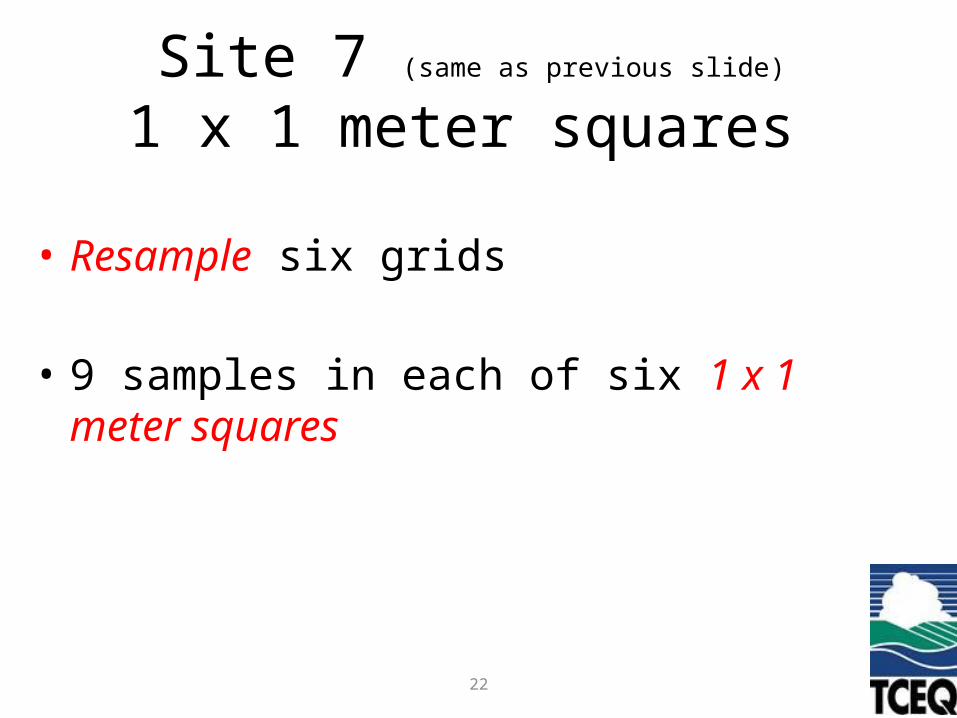
Site 7 (same as previous slide)

1 x 1 meter squares

• Resample six grids

• 9 samples in each of six 1 x 1 meter squares

22

23

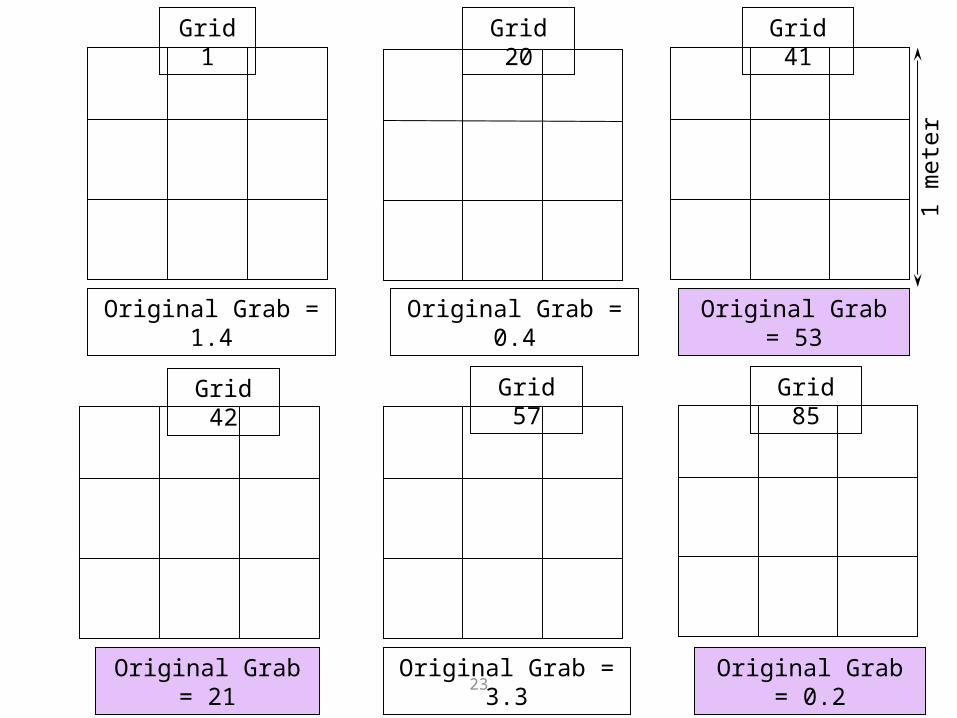
Grab Samples From Six Different Grids

Original Grab = 1.4

1 m

ete

r

Grid 1 Grid 20 Grid 41

Grid 42 Grid 57 Grid 85

Original Grab = 0.4

Original Grab = 53

Original Grab = 21

Original Grab = 3.3

Original Grab = 0.2

24

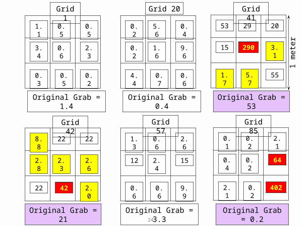
Grab Samples From Six Different Grids

1.1

3.4

0.5

0.6

0.5

0.20.50.3

2.3

0.2

0.2

5.6

1.6

0.4

0.60.74.4

9.6

0.1

0.4

0.2

0.2

2.1

4020.22.1

64

Original Grab = 1.4

1 m

ete

r

53

15

29

290

20

555.71.7

3.1

8.8

2.8

22

2.3

22

2.04222

2.6

1.3

12

0.6

2.4

2.6

9.90.60.6

15

Grid 1 Grid 20 Grid 41

Grid 42 Grid 57 Grid 85

Original Grab = 0.4

Original Grab = 53

Original Grab = 21

Original Grab = 3.3

Original Grab = 0.2

The Mean Concentration• ISM produces an estimate of the mean concentration

in the Decision Unit;

• The mean is an integral part of the framework upon which all risk-based action levels (including TRRP PCLs) are based;

• “the concentration term in the intake equation is an estimate of the arithmetic average concentration for a contaminant based on a set of site sampling results”.

• (EPA: Supplemental Guidance to RAGS: Calculating the Concentration Term)

25

The Mean Concentration 2

• The basis of most environmental decision criteria.

– EPA Risk-based Soil Screening Levels

– Groundwater Protection Levels

– Background values

– TRRP PCLs

26

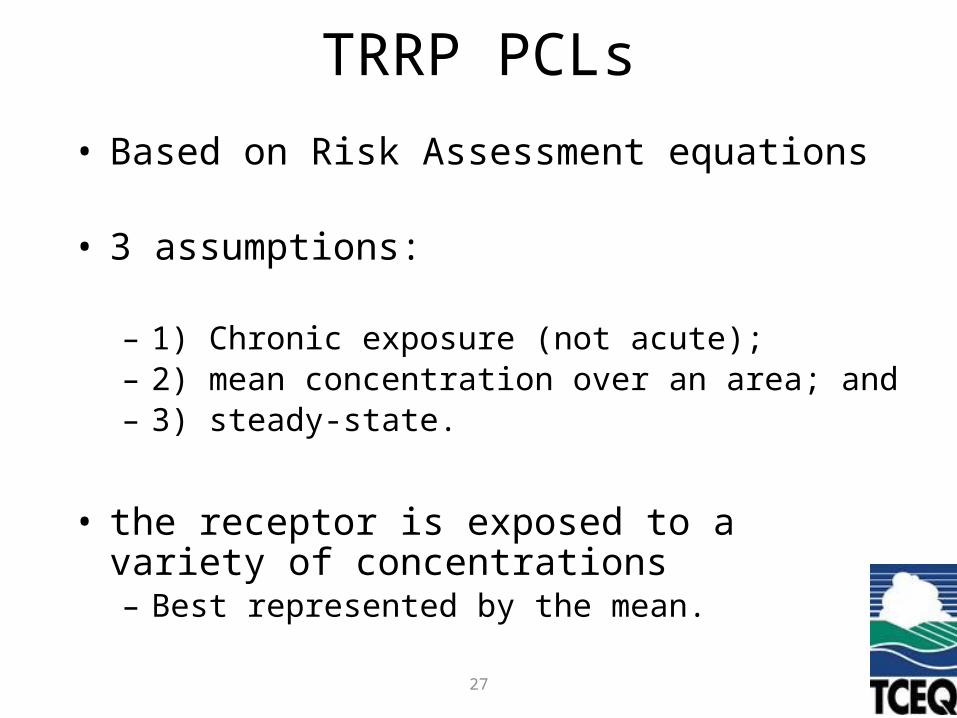
TRRP PCLs

• Based on Risk Assessment equations

• 3 assumptions:

– 1) Chronic exposure (not acute);– 2) mean concentration over an area; and– 3) steady-state.

• the receptor is exposed to a variety of concentrations– Best represented by the mean.

27

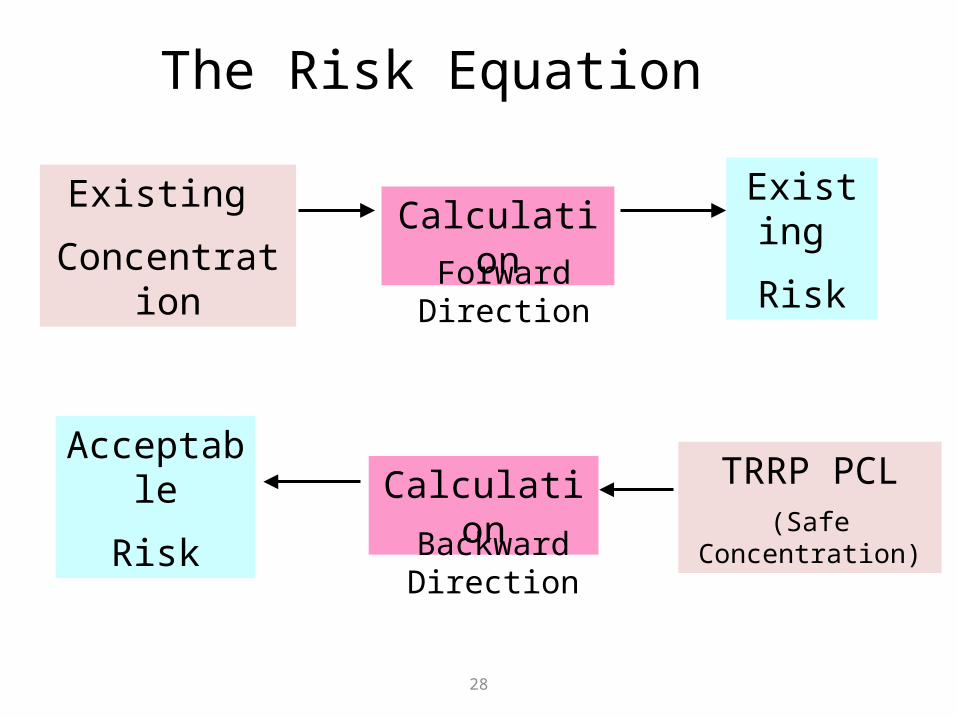
The Risk Equation

Existing

Risk

Existing

Concentration

Calculation

Forward Direction

Acceptable

Risk

TRRP PCL(Safe

Concentration)

Calculation

Backward Direction

28

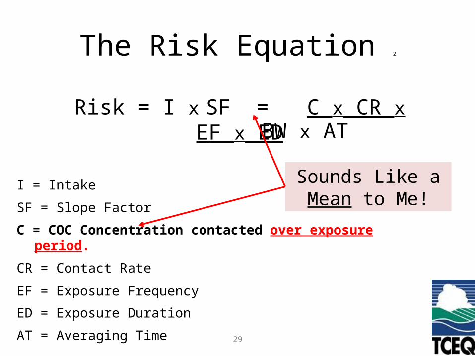
The Risk Equation 2

Risk = I x SF = C x CR x EF x ED over BW x AT

I = Intake

SF = Slope Factor

C = COC Concentration contacted over exposure period.

CR = Contact Rate

EF = Exposure Frequency

ED = Exposure Duration

AT = Averaging Time

Risk = I x SF = C x CR x EF x ED BW x AT

Sounds Like a Mean to Me!

29

TRRP and ISM• Assessment requirements under TRRP are broad

(§350.51):

– “…in a manner most likely to detect the presence and distribution of COCs…”

– “…sample collection techniques that meet the data quality needs and are acceptable to the executive director.”

– “…collection and analysis of a sufficient number of samples…”

– “…reliably characterize the nature and degree of COCs…”

– “…collect and handle samples in accordance with sampling methodologies which will yield representative concentrations of COCs present in the sampled medium.”

30

Remember!

• Heterogeneity – The largest source of decision error faced by the environmental community.

• Based on where we happen to sample!

31

Heterogeneity 2

32

ISM Implementation – The Bad News

• More increments.

• More field time per sample.

• Larger sample volume.

• Additional laboratory preparation.

33

• Fewer sample supplies.

• Less time selecting sample locations.

• Fewer locations to survey.

• No decon between increments.

• Less field documentation.

• Fewer samples to ship, prepare & analyze! 34

ISM Implementation – The Good News

ISM Results – More Good News

• More repeatable!

• More accurate!

• Better science!

• Better decisions!

35

Conclusion• ISM = cost-effective method to: –Address contaminant

heterogeneity,

–Results are:•more scientifically defensible,•more reproducible, •more representative.

–Therefore – fewer decision errors.36

ISM – Further Information• Interstate Technology & Regulatory Council (ITRC)

– 2015 Webinars• Part 1 – May 7, November 3• Part 2 – May 14, November 10.• (also see archived webinars)

• Cold Regions Research and Engineering Laboratory (CRREL) (USACE)

• EPA Clu-in– Clu-In Incremental-Composite Webinar (also see archived webinars)– Method 8330B

• Other Guidance Documents– US Army Corp of Engineers (USACE)– State of Alaska– State of Hawaii

37