Incorporating variable source area hydrology into a … · Incorporating variable source area...

HYDROLOGICAL PROCESSESHydrol. Process. 21, 3420–3430 (2007)Published online 24 July 2007 in Wiley InterScience(www.interscience.wiley.com) DOI: 10.1002/hyp.6556

Incorporating variable source area hydrology into acurve-number-based watershed model

Elliot M. Schneiderman,1* Tammo S. Steenhuis,2 Dominique J. Thongs,1 Zachary M. Easton,2

Mark S. Zion,1 Andrew L. Neal,2 Guillermo F. Mendoza1 and M. Todd Walter2

1 New York City Department of Environmental Protection, 71 Smith Avenue, Kingston, NY 12401, USA2 Department of Biological and Environmental Engineering, Cornell University, Ithaca, NY 14853, USA

Abstract:

Many water quality models use some form of the curve number (CN) equation developed by the Soil Conservation Service(SCS; U.S. Depart of Agriculture) to predict storm runoff from watersheds based on an infiltration-excess response to rainfall.However, in humid, well-vegetated areas with shallow soils, such as in the northeastern USA, the predominant runoff generatingmechanism is saturation-excess on variable source areas (VSAs). We reconceptualized the SCS–CN equation for VSAs, andincorporated it into the General Watershed Loading Function (GWLF) model. The new version of GWLF, named the VariableSource Loading Function (VSLF) model, simulates the watershed runoff response to rainfall using the standard SCS–CNequation, but spatially distributes the runoff response according to a soil wetness index. We spatially validated VSLF runoffpredictions and compared VSLF to GWLF for a subwatershed of the New York City Water Supply System. The spatialdistribution of runoff from VSLF is more physically realistic than the estimates from GWLF. This has important consequencesfor water quality modeling, and for the use of models to evaluate and guide watershed management, because correctlypredicting the coincidence of runoff generation and pollutant sources is critical to simulating non-point source (NPS) pollutiontransported by runoff. Copyright 2007 John Wiley & Sons, Ltd.

KEY WORDS curve number; variable source area hydrology; runoff; watershed modelling; General Watershed Loading Function;non-point source pollution

Received 11 July 2005; Accepted 6 July 2006

INTRODUCTION

Watershed models that simulate streamflow and pollutantloads are important tools for managing water resources.These models typically simulate streamflow components,baseflow and storm runoff, from different land areasand then associate pollutant concentrations with the flowcomponents to derive pollutant loads to streams. Stormrunoff is the primary transport mechanism for manypollutants that accumulate on or near the land surface.Accurate simulation of pollutant loads from different landareas therefore depends as much on realistic predictionsof runoff source area locations as on accurate predictionsof storm runoff volumes from the source areas.

The locations of runoff production in a watersheddepend on the mechanism by which runoff is gener-ated. Infiltration-excess runoff, also called Hortonian flow(e.g. Horton 1933, 1940), occurs when rainfall inten-sity exceeds the rate at which water can infiltrate thesoil. Soil infiltration rates are controlled by soil char-acteristics, vegetation and land use practices that affectthe infiltration characteristics of the soil surface. Incontrast, saturation-excess runoff occurs when rain (orsnowmelt) encounters soils that are nearly or fully sat-urated due to a perched water table that forms when

* Correspondence to: Elliot M. Schneiderman, New York City Depart-ment of Environmental Protection, 71 Smith Avenue, Kingston, NY12401, USA. E-mail: [email protected]

the infiltration front reaches a zone of low transmission(USDA-SCS, 1972). The locations of areas generatingsaturation-excess runoff, typically called variable sourceareas (VSAs), depend on topographic position in thelandscape and soil transmissivity. Variable source areasexpand and contract in size as water tables rise andfall, respectively. Since the factors that control soil infil-tration rates differ from the factors that control VSAs,models that assume infiltration-excess as the primaryrunoff-producing mechanism will depict the locations ofrunoff source areas differently than models that assumesaturation-excess.

In humid, well-vegetated areas with shallow soils,such as the northeastern USA, infiltration-excess doesnot always explain observed storm runoff patterns. Forshallow soils characterized by highly permeable topsoilunderlain by a dense subsoil or shallow water table, infil-tration capacities are generally higher than rainfall inten-sity, and storm runoff is usually generated by saturation-excess on VSAs (Dunne and Leopold, 1978; Beven,2001; Srinivasan et al., 2002; Needleman et al., 2004).Walter et al. (2003) found that rainfall intensities inthe Catskill Mountains, NY, rarely exceeded infiltrationrates, concluding that infiltration-excess is not a dominantrunoff generating mechanism in these watersheds.

The Generalized Watershed Loading Function (GWLF)model (Haith and Shoemaker 1987, Schneiderman et al.,2002) uses the U.S. Department of Agriculture (USDA)

Copyright 2007 John Wiley & Sons, Ltd.

WATERSHED MODELING AND VARIABLE SOURCE AREA 3421

Soil Conservation Service (SCS, now NRCS) runoff-curve-number (CN) method (USDA-SCS, 1972) to esti-mate storm runoff for different land uses or hydrologicalresponse units (HRUs). The GWLF model, like manycurrent water quality models, uses the SCS–CN runoffequation in a way that implicitly assumes that infiltration-excess is the runoff mechanism. In short, each HRU ina watershed is defined by land use and a hydrologicalsoil group classification via a ‘CN value’ that determinesrunoff response. Curve number values for different landuse and hydrological soil group combinations are pro-vided in tables compiled by USDA (e.g. USDA-SCS,1972, 1986). The hydrological soil groups used to clas-sify HRUs are based on infiltration characteristics ofsoils (e.g. USDA-NRCS, 2003) and thus clearly assumeinfiltration-excess as the primary runoff-producing mech-anism (e.g. Walter and Shaw, 2005).

Here, we describe a new version of GWLF termedthe Variable Source Loading Function (VSLF) modelthat simulates the aerial distribution of saturation-excessrunoff within the watershed. The VSLF model simu-lates runoff volumes for the entire watershed using theSCS–CN method, but spatially distributes the runoffresponse according to a soil wetness index as opposed toa combination of land use and hydrological soil group aswith the GWLF model. We review the SCS–CN methodand the theory behind the application of the SCS–CNequation to VSAs, validate the spatial predictions madeby VSLF, and compare model results between GWLFand VSLF for a watershed in the Catskill Mountains ofNew York State to demonstrate differences between thetwo approaches.

REVIEW OF THE SCS–CN METHOD

The SCS–CN method estimates total watershed runoffdepth Q (mm) for a storm by the SCS runoff equation(USDA-SCS, 1972):

Q D �Pe�2

�Pe C Se��1�

where Pe (mm) is the depth of effective rainfall afterrunoff begins and Se (mm) is the depth of effective avail-able storage (mm), i.e. the spatially averaged availablevolume of retention in the watershed when runoff begins.We use the term effective and the subscript ‘e’ to iden-tify parameter values that refer to the period after runoffstarts. Although Se in Equation (1) is typically writtensimply as S, this term is clearly defined for when runoffbegins as opposed to when rainfall begins (USDA-SCS,1972); thus we refer to it as Se.

At the beginning of a storm event, an initial abstraction,Ia (mm), of rainfall is retained by the watershed prior tothe beginning of runoff generation. Effective rainfall, Pe,and storage, Se, are thus (USDA-SCS, 1972):

Pe D P � Ia �2a�

Se D S � Ia �2b�

where P (mm) is the total rainfall for the storm event andS (mm) is the available storage at the onset of rainfall.In the traditional SCS–CN method, Ia is estimated as anempirically derived fraction of available storage:

Ia D 0Ð2 Se �3�

Effective available storage, Se, depends on the moisturestatus of the watershed and can vary between somemaximum Se,max (mm) when the watershed is dry, e.g.during the summer, and a minimum Se,min (mm) whenthe watershed is wet, usually during the early spring.The Se,max and Se,min limits have been estimated to varyaround an average watershed moisture condition withcorresponding Se,avg (mm) based on empirical analysis ofrainfall-runoff data for experimental watersheds (USDA-SCS, 1972; Chow et al., 1988):

Se,max D 2Ð381 Se,avg �4�

Se,min D 0Ð4348 Se,avg �5�

Se,avg is determined via table-derived CN values foraverage watershed moisture conditions (CNII) and astandard relationship between Se and CNII.

Se,avg D 254(

100

CNII � 1

)�6�

However, for most water quality models, Se,avg (mm) isultimately a calibration parameter that is only looselyconstrained by the USDA-CN tables. Values for CNII andSe,avg can be derived directly from baseflow-separatedstreamflow data when such data are available (USDA-NRCS, 1997; NYC DEP, 2006).

In the original SCS–CN method, Se varies dependingon antecedent moisture or precipitation conditions of thewatershed (USDA-SCS, 1972). For VSA watersheds, apreferred method varies Se directly with soil moisturecontent. We use a parsimonious method adapted fromthe USDA soil-plant-atmosphere-water (SPAW) model(Saxton et al. 1974). The value of Se is set to Se,min whenunsaturated zone soil water is at or exceeds field capacity,and is set to Se,max when soil water is less than or equalto a fixed fraction of field capacity (a parameter termedspaw cn coeff in VSLF), which is set to 0Ð6 in the SPAWmodel but can be calibrated in VSLF. The value for Se isderived by linear interpolation when soil water is betweenSe,min and Se,max thresholds.

SCS–CN EQUATION APPLIED TO VSA THEORY

The SCS–CN equation, Equation (1), constitutes anempirical runoff–rainfall relationship. It is therefore inde-pendent of the underlying runoff generation mecha-nism, i.e. infiltration-excess or saturation-excess. In fact,the originator of Equation (1), Victor Mockus (Rallison1980), specifically noted that Se is either ‘controlledby the rate of infiltration at the soil surface or by the

Copyright 2007 John Wiley & Sons, Ltd. Hydrol. Process. 21, 3420–3430 (2007)DOI: 10.1002/hyp

3422 E. M. SCHNEIDERMAN ET AL.

rate of transmission in the soil profile or by the water-storage capacity of the profile, whichever is the lim-iting factor’ (USDA-SCS, 1972). Interestingly, in lateryears he reportedly said ‘saturation overland flow wasthe most likely runoff mechanism to be simulated by themethod. . .’ (Ponce, 1996).

Steenhuis et al. (1995) showed that Equation (1) couldbe interpreted in terms of a saturation-excess process.Assuming that all rain falling on unsaturated soil infil-trates and that all rain falling on areas that are saturated(to the surface or to a near-surface preferential flow zone)becomes runoff, then the rate of runoff generation willbe proportional to the fraction of the watershed that iseffectively saturated, Af, which can then be written as:

Af D Q

Pe�7�

where Q is incremental saturation-excess runoff or,more precisely, the equivalent depth of excess rainfallgenerated during a time period over the whole watershedarea, and Pe is the incremental depth of precipitationduring the same time period. We define saturation-excessrunoff Q in Equation (7) to include both overland flowwhere soil is saturated to the surface and rapid subsur-face flow due to a perched water table intersecting anupper soil layer where preferential flow (i.e. unimpededsubsurface lateral flow through macropores) exists. If Qincludes runoff generated by other mechanisms (e.g. infil-tration excess runoff) then Af may be overestimated. Inwhat follows Q is exclusively saturation-excess runoff.

By writing the SCS Runoff Equation (1) in differentialform and differentiating with respect to Pe, the fractionalcontributing area for a storm can be written as:

Af D 1 � S2e

�Pe C Se�2 �8�

According to Equation (8) runoff occurs only on areasthat have a local effective available storage �e (mm)less than Pe. Therefore by substituting �e for Pe inEquation (8) we have a relationship for the percent ofthe watershed area, As, which has a local effective soilwater storage less than or equal to �e for a given overallwatershed storage of Se:

As D 1 � S2e

��e C Se�2 �9�

Solving for �e gives the maximum effective (local) soilmoisture storage within any particular fraction As of theoverall watershed area, for a given overall watershedstorage of Se:

�e D Se

(√1

�1 � As�� 1

)�10�

or, expressed in terms of local storage, � (mm), whenrainfall begins (as opposed to when runoff begins):

� D Se

(√1

�1 � As�� 1

)C Ia �11�

Equation (11) is illustrated conceptually in Figure 1. Fora given storm event with precipitation P, the locationof the watershed that saturates first (As D 0) has localstorage � equal to the initial abstraction Ia, and runofffrom this location will be P � Ia. Successively drierlocations retain more precipitation and produce lessrunoff according to the moisture–area relationship ofEquation (11). The driest location that saturates definesthe runoff contributing area (Af) for a particular stormof precipitation P. The reader is reminded that both Se

and Ia are watershed-scale properties that are spatiallyinvariant.

As average effective soil moisture (Se) changes throughthe year, the moisture–area relationship will shift accord-ingly as per Equation (10). However, once runoff beginsfor any given storm, the effective local moisture storage,�e, divided by the effective average moisture storage,Se, assumes a characteristic moisture–area relationshipaccording to Equation (10) that is invariant from stormto storm (Figure 2).

Runoff q (mm) at a point location in the watershed cannow also be expressed for the saturated area simply as:

q D Pe � �e for Pe > �e �12�

and for the unsaturated portion of the watershed:

q D 0 for Pe � �e �13�

The total runoff Q of the watershed can be expressed asthe integral of q over Af.

Q D∫ Af

0q�dAs� �14�

Transforming GWLF into VSLF

The GWLF model calculates runoff by applyingEquation (1) separately for individual HRUs, which aredistinguished by infiltration characteristics of soils andland use. The VSLF model simulates runoff from

As

σ

P

Ia

Af

Q

0 0.2 0.4 0.6 0.80

50

100

150

200

250

1

Retained

Figure 1. Relationship of available local moisture storage, �, to thefraction of watershed area contributing runoff (As)



0

1

2

3

4

5

6

7

8

9

10

0 0.2 0.4 0.6 0.8

As

σ e /S

e

1

Figure 2. Relationship of effective local moisture storage, �e, normalizedto effective average moisture storage Se, to the fraction of watershed area

contributing runoff (As)

HRUs dominated by impervious surfaces with the sameinfiltration-excess approach used in GWLF. The remain-ing watershed area, consisting of pervious surfaces, istreated according to the VSA CN theory developed.

In VSLF, determination of runoff from HRUs isbased on a soil wetness index that classifies each unitarea of a watershed according to its relative propensityfor becoming saturated and producing saturation-excessstorm runoff. Here we propose using the soil topographicindex from TOPMODEL (Beven and Kirkby, 1979) todefine the distribution of wetness indices, although VSLFdoes not require any specific index. A soil topographicindex map of a watershed is generated by dividing thewatershed into a grid of cells and calculating the indexfor each cell by:

� D ln(

a

T tan ˇ

)�15�

where a is the upslope contributing area for the cell perunit of contour line (m), tan ˇ is the topographic slopeof the cell and T is the transmissivity at saturation of theuppermost layer of soil (m2 day�1)—calculated from soilsurvey data as the product of soil depth and saturatedhydraulic conductivity. This formulation neglects theimpact of land use, a simplification based on the logicthat, in general, there is no need for a separate waterbalance for each land use when saturation excess runoff isthe dominant process. This assumption may cause someerrors in the summer period for some land-cover typeswhen evapotranspiration is significant, but is generallynot believed to be troublesome.

The wetness index is used to qualitatively rank areasor HRUs in the watershed in terms of their overallprobability of runoff. The number and/or size of the indexclasses depend upon the application of the user. As anexample, we chose to divide the watershed into ten equal-area classes according to the wetness index, i.e. class 1as the wettest 10% of the watershed, class 2 as the next

wettest 10%, etc. The effective soil water storage withineach area is determined by integrating Equation (10):

�e,i D∫ As,iC1

As,i

�eÐdAs

D 2Se�√

1 � As,i � √1 � As,iC1�

�As,iC1 � As,i�� Se �16�

where each wetness class area is bounded on one sideby the fraction of the watershed that is wetter, As,i,i.e., the part of the watershed that has lower localmoisture storage, and on the other side by the fractionof the watershed that is dryer, As,iC1, i.e., has greaterlocal moisture storage. A wetness index class defined inthis way may coincide with multiple land uses. Runoffdepth within an index class in VSLF will be the sameirrespective of land use, but nutrient concentrations areassigned to land uses independent of wetness class.Wetness index classes are thus subdivided by land useto define HRUs with unique combinations of wetnessclass and land use. Nutrient loads from each wetness-class–land-use HRU are tracked separately in VSLF, butotherwise are estimated as in GWLF.

In the original GWLF, runoff is calculated for eachsoil- and land-use-defined HRU using Equation (1).In VSLF, when precipitation occurs the contributingarea fraction, Af, is first calculated with Equation (8).Runoff is then calculated for each wetness class withEquations (12) and (13), where �e is determined byEquation (16). For the entire watershed, runoff depth Qis the aerially weighted sum of runoff depths qi for alldiscrete contributing areas:

Q Dn∑

iD1

qi�As,iC1 � As,i� �17�

The total runoff depth, Q, calculated by this equationis the same as that calculated by the SCS runoffEquation (1). The main difference between the VSLFand GWLF approaches to utilizing the SCS runoffequation is that runoff is explicitly attributable to sourceareas according to a wetness index distribution (e.g.Equation 15), rather than by land use and soil infiltrationproperties as in original GWLF. Soil properties that con-trol saturation-excess runoff generation (saturated con-ductivity, soil depth) affect runoff distribution in VSLFsince they are included in the wetness index.

VSLF VALIDATION

Both the integrated and distributed VSLF predictionswere tested to assess its applicability to temperate, north-eastern USA watersheds. Three different tests were per-formed: (1) we compared predicted and observed basin-scale runoff; (2) we compared the locations of VSLFpredicted saturated areas to those predicted by a more rig-orous physically based model, Soil Moisture Distributionand Routing (SMDR;e.g. Frankenberger et al., 1999); and



Figure 3. Location Map of the Cannonsville watershed

(3) we compared predicted and field-measured soil mois-ture over several transects.

These tests were performed within the CannonsvilleReservoir watershed located in the Catskill Mountainregion of New York State. The Cannonsville is one ofthe reservoirs that supply water to New York City. Ithas a watershed area of 1180 km2 and is predominatelyforested or agricultural land with moderate to steep hill-slopes and mostly shallow soils overlying glacial till orbedrock (Schneiderman et al., 2002). The Cannonsvillewatershed upstream of the U.S. Geological Survey gaug-ing station at West Branch Delaware River (WBDR) atWalton was used for test (1) and a small sub-basin wasused for (2) and (3) (Figure 3).

For VSLF application, a wetness index map for thewatershed of interest was created with ten equal-areaindex classes. A soil topographic index map at a 30 mgrid cell resolution was made using Equation (15). The‘a’ values for Equation (15) were determined using amultidirectional flow path algorithm (Thongs and Wood,1993). Soil depths and saturated conductivity values,required to calculate T (Equation 15), were obtained fromU.S. Department of Agriculture Soil Survey Geographic(SSURGO) data. The soil topographic index map datawere then aggregated to create a map of ten equal-areaindex classes, the wettest class being the 10% of thewatershed with the highest topographic index values (i.e.corresponding to the wettest 10%), the next wettest classbeing the 10–20% range of next highest index values,and so on. The wetness index map was then intersectedwith a land use map, based on 1992 LANDSAT data, toderive areas for each wetness-index–land-use HRU.

Test 1

The VSLF model was applied to the Cannonsvillewatershed upstream of the WBDR at Walton U.S.geological Survey gauging station. A previous study(NYC DEP, 2006) developed and applied a methodol-ogy for calibrating the watershed Se,avg in GWLF againstobserved runoff estimates from baseflow-separated dailystream hydrograph data. The model was calibrated for1992–1999 and a leave-one-out cross validation (loocv)time series (McCuen, 2005) that is independent of the cal-ibration was developed for comparison with 1992–1999data. Figure 4a shows the VSLF simulated event runoff(loocv time series) plotted against observed runoff lossesat WBDR at Walton. Event runoff is defined as the directrunoff component of the baseflow-separated daily hydro-graph, summed over a period that lasts from the firstday of streamflow hydrograph rise until the beginningof the next event. The VSLF simulations of watershedrunoff volumes for this period agree well with observedrunoff data at the watershed outlet. Nash–Sutcliff effi-ciency (Nash and Sutcliffe, 1970) (E) was E D 0Ð86. Nosystematic bias was evident in the results, with predictedversus observed data evenly scattered around the 1 : 1 line(Figure 4B).

Test 2

Figure 5 shows the spatial probability of saturatedareas using VSLF and SMDR for a small sub-watershed.Probability of saturation was defined as the ratio of the‘number of days for which a location (or wetness classfor VSLF) is saturated’ to the ‘total number of dayssimulated’ (e.g. Walter et al., 2000, 2001). The VSLF



Year

120

60

01992 1993 1994 1995 1996

Run

off (

mm

)

Measured

Predicted

120

60

Year

Run

off (

mm

)

1996 1997 1998 1999 20000

Measured

Predicted

120

90

60

30

120906030

Measured (mm)

Pre

dict

ed (

mm

)

00

(b)

(a)

Figure 4. (A) Observed and VSLF-simulated event runoff (mm) from the Cannonsville watershed, and (B) scatterplot of observed versus predictedevent runoff for 1992–1999. Observed event runoff estimated by baseflow separation of daily streamflow hydrograph. Nash–Sutcliffe efficiency was

0Ð86

VSLF Saturation Probability0 - 0.10.1 - 0.20.2 - 0.30.3 - 0.40.4 - 0.50.5 - 0.60.6 - 0.70.7 - 0.80.8 - 0.90.9 - 1

SMDR Saturation Probability

0 - 0.10.1 - 0.20.2 - 0.30.3 - 0.40.4- 0.50.5 - 0.60.6 - 0.70.7 - 0.80.8 - 0.90.9 - 1

Figure 5. Probability of saturation for runoff-event predictions for a Cannonsville subwatershed using VSLF model and the Soil Moisture Distributionand Routing (SMDR) model. Soil moisture sampling transects used in Figure 6 are shown on the VSLF map

results showed similar patterns of predicted saturationas SMDR (Figure 5), which has been extensively andsuccessfully tested in this watershed (e.g. Frankenbergeret al., 1999; Mehta et al., 2004; Gerard-Marchant et al.,2005). It is perhaps not surprising that these two modelsagree so strongly since both SMDR and topographicindex are strongly driven by topography. Thus, both

show higher probability of saturation in the downslopeareas where slopes flatten and where there is a largeupslope contributing area. In both models the areas of lowprobability of saturation coincide with the upslope areas.There are a few differences between the distributions ofsaturated areas predicted by the two models (Figure 5).The VSLF model shows continuity in the distribution



of saturated areas in the landscape, whereas SMDR,due to the process based computation, better predictsdiscontinuous saturated areas. In general, the standarderror between predicted saturated area using VSLF andSMDR varied by <5%; a small fraction (<10%) hadlarger differences, e.g. the pond in the middle of thewatershed could have been better predicted in VSLF witha few modifications.

Test 3

We used observed saturation degree data from Franken-berger et al. (1999) and Gerard-Marchant et al. (2005);the transect locations are shown in Figure 5. For eachtransect location the predicted saturation degree, sd, wascalculated from the estimated moisture deficit (i.e. avail-able local storage �, Equation 11) and soil pore volume,Vf (mm), for that location:

sd D 1 � �/Vf �18�

Figure 6 shows examples of the simulated and observedsaturation degree for three transects and two dates (6May 1994 and 8 June 2001). The two lines showingthe simulated results in Figure 6 represent the saturationdegree when rainfall starts (dashed line, Equation 11)and when runoff is initiated (solid line, Equation 10). Onboth dates and all three transects, the simulated saturationdegree show good agreement with the measured data.Most of the observed values fall between the simulatedsaturation degree estimates (Figure 6). Since variabilityin field soils is high, especially over 10 ð 10 m grids, wehave shown the sampling error (or variability) associatedwith each of the measured points as a shaded band(Gerard-Marchant et al., 2005). For every sampling point,at least one of the predicted upper and lower saturationdegrees lies within the band representing error estimatesof the observed data. Thus, the observed and simulatedvalues differ by similar or smaller magnitudes than theerror or variability seen in the field.

Figure 7 shows the grouped comparison of the satu-ration degree from five transects and three dates. Sincemultiple observed points along the transect fall within asingle index class, the mean of the observed saturationdegree for each index class was used in the comparison.The horizontal error bars show the standard error of therange of observed values for each mean, and allow com-parison of the inherent variability of soil moisture levelsbetween transects. Overall, the saturation degree was wellpredicted by the model, with coefficient of determinationr2 D 0Ð76 and E D 0Ð70. The outlier in Figure 7 is from alate October sample when the model predicted drier con-ditions than observed due to underestimation of autumnprecipitation for the subwatershed where the transectsare located. This outlier strongly influences the regres-sion, skewing the intercept term. Removing this pointresults in a slope D 1Ð08, and the r2 increases to 0Ð79, andE D 0Ð76. The VSLF predicted saturation degree accu-racy is comparable to that predicted by fully distributed,process-based models such as SMDR.

Figure 6. Observed and simulated soil moisture levels at the initiationof rainfall (long dashed line) and runoff (solid line) from three transectsin the watershed. Grey area represents observed sampling error. Shortvertical dashed line represents a transition between wetness index classes

based on the topographic index

SPATIAL DISTRIBUTION OF RUNOFF IN VSLFVERSUS GWLF

We applied both GWLF and VSLF models to the WBDRat Walton watershed, upstream of the Cannonsville Reser-voir, to compare spatial patterns of runoff as predicted bythe two models. The GWLF model was applied using theSPAW method for varying Se with soil moisture and thecalibrated parameters from the VSLF model application(test 1 above), to be consistent with the VSLF applica-tion to WBDR at Walton. Runoff at the watershed outletpredicted with the two models is very similar (Figure 8).



Observed Saturation Degree (cm3 cm-3)

Sim

ulat

ed S

atur

atio

n D

egre

e (c

m3

cm-3

)

0.4

0.6

0.8

1.0Saturation Degree

y = 1.4x - 0.23r2 = 0.7695% PredictionIntervals

0.4 0.6 0.8 1.0

Figure 7. Scatter plot of observed and the Variable Source LoadingFunction (VSLF) model simulated soil moisture levels from five dates andthree transects in both the growing and dormant seasons in the R-Farmsubwatershed. Since numerous observed values fall within the same indexclass along the transect, the mean observed value was regressed againsteach individual index class. Horizontal bars represent the standard error

of the observed saturation degree for each index class

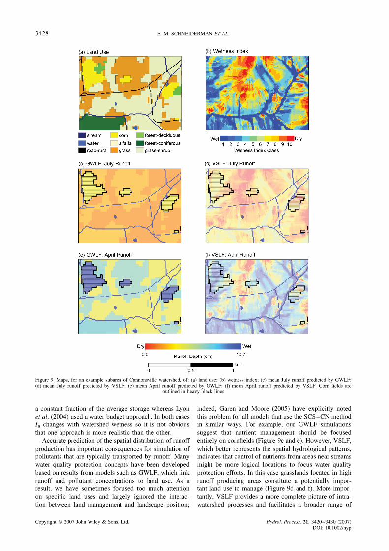
Slight differences are due to the fact that VSLF calcu-lates runoff for the total pervious area of the watershedusing a single parameter (Se,avg), whereas GWLF cal-culates runoff separately for each individual land use.The spatial distribution of runoff predicted by VSLF andGWLF is, as expected, markedly different. The GWLFrunoff predictions are controlled by the spatial patternof land use and, to a lesser degree, soils, whereas VSLFrunoff predictions follow the pattern of the wetness index.Figure 9a and b depicts the land use map and wetnessindices, respectively, for an example subarea of Can-nonsville watershed. Figure 9c–f shows how the under-lying spatial patterns in Figure 9a and b correspond tothe distribution of runoff predictions. Depicted are aver-age runoff predictions over the simulation period for adry period of the year, July, and a wet period of the year,April. For both models, there is overall more runoff gen-erated in April, when watershed moisture conditions arewettest, than in July. However, GWLF predicts that mostof the runoff comes from cornfields and predicts all corn-fields generate runoff equally (Figure 9c and e); indeed,any given land use has uniform runoff predicted from itregardless of its location in the watershed. This, of course,follows from the fact that the original GWLF model, likemost water quality models, use tabulated Se,avg (or CNII)values based on tables that correlate runoff response toland use and soil type. For example, on these tables,cornfields have one of the highest runoff responses, i.e.,lowest Se,avg (highest CNII). In contrast, the spatial pat-tern of runoff predicted by VSLF follows the pattern ofthe wetness index, with high wetness index areas generat-ing most of the runoff; compare Figure 9b with 9d and f.

DISCUSSION

The model developed here is essentially an amalgam ofVSA ideas that have been developed over the past sev-eral years. For example, wetness indices have been used

0

1

2

3

0 2

VSLF Runoff (cm)

GW

LF R

unof

f (cm

)

r2=0.99

1 3

Figure 8. Scatter plot of the Generalized Watershed Loading Function(GWLF) model versus the Variable Source Loading Function (VSLF)

model simulated event runoff for the Cannonsville watershed

to effectively predict VSAs for watersheds dominated bysaturation-excess runoff (e.g. Western et al., 1999), andtopographic indices have been used outside the TOP-MODEL (Beven and Kirkby, 1979) framework to predictVSAs (e.g. Lyon et al., 2004; Agnew et al., 2006). Byusing a wetness index to spatially distribute runoff, theVSLF model more realistically predicts the locations ofrunoff production in saturation-excess dominated water-sheds than the original GWLF model, which distributesrunoff by land use and soil infiltration rate (Figure 9).Thus it follows that the distribution of runoff genera-tion in VSLF agrees conceptually with the our scientificunderstanding of VSA hydrology (e.g. Hewlett and Hib-bert, 1967; Dunne and Black, 1970; Dunne and Leopold,1978; Frankenberger et al., 1999; Western et al., 1999,2004; Beven, 2001; Mehta et al., 2004; Niedzialek andOgden, 2004).

The application of the SCS–CN method to VSAspresented here is an extension of the ideas proposedby Steenhuis et al. (1995) and, especially, Lyon et al.(2004). Lyon et al. (2004) used Equation (8) to deter-mine the fraction of the watershed contributing for agiven effective precipitation and identified the specificcontributing area via a topographic index, Equation (15).Lyon et al. (2004) assumed that after runoff started therewas only one storage parameter S for the whole watershedindependent of initial wetness. In the new version pre-sented here, S is a function of overall watershed wetness,which is a conceptual improvement over the constant Sapproach used by Steenhuis et al. (1995) and Lyon et al.(2004). In addition, the method presented here predictsspatially variable runoff depths within a saturated area,whereas the Lyon et al. (2004) approach assigns a sin-gle runoff depth to the entire saturated area. Since thisis an average depth, the Lyon et al. (2004) approach willunderpredict the amount of runoff generated near streams,which may be a critical area of non-point contaminantloading in many watersheds. Some other minor differ-ences between the Lyon et al. (2004) approach and thenew version are that the initial abstraction used here is



Figure 9. Maps, for an example subarea of Cannonsville watershed, of: (a) land use; (b) wetness index; (c) mean July runoff predicted by GWLF;(d) mean July runoff predicted by VSLF; (e) mean April runoff predicted by GWLF; (f) mean April runoff predicted by VSLF. Corn fields are

outlined in heavy black lines

a constant fraction of the average storage whereas Lyonet al. (2004) used a water budget approach. In both casesIa changes with watershed wetness so it is not obviousthat one approach is more realistic than the other.

Accurate prediction of the spatial distribution of runoffproduction has important consequences for simulation ofpollutants that are typically transported by runoff. Manywater quality protection concepts have been developedbased on results from models such as GWLF, which linkrunoff and pollutant concentrations to land use. As aresult, we have sometimes focused too much attentionon specific land uses and largely ignored the interac-tion between land management and landscape position;

indeed, Garen and Moore (2005) have explicitly notedthis problem for all models that use the SCS–CN methodin similar ways. For example, our GWLF simulationssuggest that nutrient management should be focusedentirely on cornfields (Figure 9c and e). However, VSLF,which better represents the spatial hydrological patterns,indicates that control of nutrients from areas near streamsmight be more logical locations to focus water qualityprotection efforts. In this case grasslands located in highrunoff producing areas constitute a potentially impor-tant land use to manage (Figure 9d and f). More impor-tantly, VSLF provides a more complete picture of intra-watershed processes and facilitates a broader range of



potentially important NPS pollution processes. It shouldprobably be noted that the original GWLF (Haith andShoemaker, 1987) was not designed to give this levelof spatially explicit detail, and VSLF represents the waythat models may be diverted over time from their originalscope of purpose (e.g. Garen and Moore, 2005; Walterand Shaw, 2005).

CONCLUSIONS

The SCS–CN method for estimating runoff is used inmany current non-point-source pollution models to simu-late infiltration-excess runoff. These models assume thatrunoff generation and pollutant loading are tightly linkedto land use, and other factors that directly impact soilinfiltration capacity. For humid, well-vegetated water-sheds, however, saturation-excess on VSAs is the pre-dominant runoff mechanism, and runoff generation ismore indicative of landscape position than land use. Wedescribe an alternative SCS–CN-based approach to pre-dicting runoff that is applicable to VSA watersheds andshould be relatively easy to implement in existing models.We spatially validated the predictions made by the modeland, as a demonstration, showed that in watersheds wheresaturation-excess is the dominant runoff process the newVSLF model provides a much more valid spatial distri-bution of runoff generation than current SCS–CN-basedwater quality models.

ACKNOWLEDGEMENTS

We would like to acknowledge our reviewers, one ofwhich pointed out that that variable source areas donot have to be saturated to the surface to producerunoff. This is correct and has led us to redefine thedefinition of storm runoff and variable source areas. Otherreviewers also made very helpful comments and due totheir efforts the manuscript has improved greatly. TheUSDA-CSREES, USDA-NRI, and NSF-REU programspartially funded the involvement of the Soil and WaterLaboratory from Cornell’s Biological and EnvironmentalEngineering Department.

REFERENCES

Agnew LJ, Lyon S, Gerard-Marchant P, et al. 2006. Identifyinghydrologically sensitive areas: Bridging science and application.Journal of Environmental Management 78: 64–76.

Beven K. 2001. Rainfall–Runoff Modeling: The Primer . Wiley:Chichester; 360 pp.

Beven KJ, Kirkby MJ. 1979. A physically-based, variable contributingarea model of basin hydrology. Hydrological Science Bulletin 24:43–69.

Chow VT, Maidment DR, Mays LW. 1988. Applied Hydrology .McGraw-Hill: New York; 572 pp.

Dunne T, Black RD. 1970. Partial area contributions to storm runoffin a small New England watershed. Water Resources Research 6:1296–1311.

Dunne T, Leopold L. 1978. Water in Environmental Planning . W.H.Freeman: New York; 818 pp.

Frankenberger JR, Brooks ES, Walter MT, Walter MF, Steenhuis TS.1999. A GIS-based variable source area model. Hydrological Processes13(6): 804–822.

Garen DC, Moore DS. 2005. Curve number hydrology in water qualitymodeling: uses, abuses, and future directions. Journal of the AmericanWater Resources Association 41(2): 377–388.

Gerard-Marchant P, Hively WD, Steenhuis TS. 2005. Distributedhydrological modeling of total dissolved phosphorus transport in anagricultural landscape, part I: distributed runoff generation. Hydrologyand Earth Systems Science Discussions 2: 1537–1579.

Haith DA, Shoemaker LL. 1987. Generalized Watershed LoadingFunctions for stream flow nutrients. Water Resources Bulletin 23(3):471–478.

Hewlett JD, Hibbert AR. 1967. Factors affecting the response of smallwatersheds to precipitation in humid regions. In Forest Hydrology ,Sopper WE, Lull HW (eds). Pergamon Press: Oxford; 275–290.

Horton RE. 1933. The role of infiltration in the hydrologic cycle. Eos(Transactions of the American Geophysical Union) 14: 44–460.

Horton RE. 1940. An approach toward a physical interpretation ofinfiltration-capacity. Soil Science Society of America Proceedings 5:399–417.

Lyon SW, Walter MT, Gerard-Marchant P, Steenhuis TS. 2004. Using atopographic index to distribute variable source area runoff predictedwith the SCS curve-number equation. Hydrological Processes 18(15):2757–2771.

McCuen RH. 2005. Accuracy assessment of peak discharge models.Journal of Hydrologic Engineering 10(1): 16–22.

Mehta VK, Walter MT, Brooks ES, et al. 2004. Evaluation andapplication of SMR for watershed modeling in the Catskill Mountainsof New York State. Environmental Modeling and Assessment 9(2):77–89.

Nash JE, Sutcliffe JV. 1970. River flow forecasting through conceptualmodels, Part 1—a discussion of principles. Journal of Hydrology 10:282–290.

Needleman BA, Gburek WJ, Petersen GW, Sharpley AN, Kleinman PJA.2004. Surface runoff along two agricultural hillslopes with contrastingsoils. Soil Science Society of America Journal 68: 914–923.

NYC DEP. 2006. New York City’s 2006 Watershed ProtectionProgram Summary and Assessment, Appendix 4: Cannonsville GWLFModel Calibration and Validation. New York City Department ofEnvironmental Protection: Valhalla, New York.

Niedzialek JM, Ogden FL. 2004. Numerical investigation of saturatedsource area behavior at the small catchment scale. Advances in WaterResources 27(9): 925–936.

Ponce VM. 1996. Notes of my conversation with Vic Mockus.http://mockus.sdsu.edu.

Rallison RE. 1980. Origin and evolution of the SCS runoff equation.Symposium on Watershed Management , American Society of CivilEngineers: New York, NY; 912–924.

Saxton KE, Johnson HP, Shaw RH. 1974. Modeling evaptranspirationand soil moisture. Transactions of the American Society of AgriculturalEngineers 17(4): 673–677.

Schneiderman EM, Pierson DC, Lounsbury DG, Zion MS. 2002. Mod-eling the hydrochemistry of the Cannonsville Watershed with General-ized Watershed Loading Functions (GWLF). Journal of the AmericanWater Resources Association 38(5): 1323–1347.

Srinivasan MS, Gburek WJ, Hamlett JM. 2002. Dynamics of stormflowgeneration—a field study in east-central Pennsylvania, USA.Hydrological Processes 16(3): 649–665.

Steenhuis TS, Winchell M, Rossing J, Zollweg JA, Walter MF. 1995.SCS runoff equation revisited for variable-source runoff areas.American Society of Civil Engineers, Journal of Irrigation andDrainage Engineering 121: 234–238.

Thongs DJ, Wood E. 1993. Comparison of topographic soil indexesderived from large and small scale digital elevation models for differenttopographic regions. Presented at American Geophysical Union SpringMeeting, Baltimore, MD.

USDA-NRCS. 1997. National Engineering Handbook , Part 630Hydrology, Section 4, Chapter 5. Natural Resources ConservationService, U.S. Department of Agriculture.

USDA-NRCS. 2003. National Soil Survey Handbook, title 430-VI. NaturalResources Conservation Service, U.S. Department of Agriculture.http://soils.usda.gov/technical/handbook/.

USDA-SCS. 1972. National Engineering Handbook , Part 630 Hydrology,Section 4, Chapter 10. Natural Resources Conservation Service, U.S.Department of Agriculture.

USDA-SCS. 1986. Urban Hydrology for Small Watersheds , TechnicalRelease No. 55. Soil Conservation Service, U.S. Department ofAgriculture. U.S. Government Printing Office: Washington, DC.



Walter MT, Shaw SB. 2005. Discussion: ‘Curve number hydrology inwater quality modeling: Uses, abuses, and future directions’ by Garenand Moore. Journal of American Water Resources Association 41(6):1491–1492.

Walter MT, Walter MF, Brooks ES, Steenhuis TS, Boll J, Weiler KR.2000. Hydrologically sensitive areas: variable source area hydrologyimplications for water quality risk assessment. Journal of Soil andWater Conservation 3: 277–284.

Walter MT, Brooks ES, Walter MF, Steenhuis TS, Scott CA, Boll J.2001. Evaluation of soluble phosphorus transport from manure-appliedfields under various spreading strategies. Journal of Soil and WaterConservation 56(4): 329–336.

Walter MT, Mehta K, Marrone AM, et al. 2003. A simple estimationof the prevalence of Hortonian flow in New York City’swatersheds. American Society of Civil Engineers, Journal of HydrologicEngineering 8(4): 214–218.

Western AW, Grayson RB, Bloschl G, Willgoose GR, McMahon TA.1999. Observed spatial organization of soil moisture and its relation toterrain indices. Water Resources Research 35(3): 797–810.

Western AW, Zhou SL, Grayson RB, McMahon TA, Bloschl G, Wil-son DJ. 2004. Spatial correlation of soil moisture in small catchmentsand its relationship to dominant spatial hydrological processes. Journalof Hydrology 286(1–4): 113–134.


Incorporating variable source area hydrology into a … · Incorporating variable source area...

Documents

Transcript of Incorporating variable source area hydrology into a … · Incorporating variable source area...