Incorporating pedigree information into the analysis of ...
266
THE UNIVERSITY OF ADELAIDE Faculty of Science School of Agriculture, Food and Wine Incorporating Pedigree Information into the Analysis of Agricultural Genetic Trials Helena Oakey Doctor of Philosophy May 2008
Transcript of Incorporating pedigree information into the analysis of ...

THE UNIVERSITY OF ADELAIDE
Faculty of Science
School of Agriculture, Food and Wine
Incorporating Pedigree Information
into the Analysis of
Agricultural Genetic Trials
Helena Oakey
Doctor of Philosophy
May 2008

Contents
1 Introduction 1
1.1 A new approach to the analysis of agricultural genetic trials . . . . . . . . 13
2 Measures of Relatedness 18
2.1 Genes, alleles, genotypes and genetic effects . . . . . . . . . . . . . . . . . 19
2.2 Identity Modes . . . . . . . . . . . . . . . . . . . . . . . . . . . . . . . . . 23
2.3 Coefficient of Coancestry . . . . . . . . . . . . . . . . . . . . . . . . . . . . 26
2.4 Coefficient of Inbreeding . . . . . . . . . . . . . . . . . . . . . . . . . . . . 27
2.5 Special Case of the coefficient of Coancestry . . . . . . . . . . . . . . . . . 28
2.6 The genetic variance and covariance under inbreeding and Mendelian sam-
pling . . . . . . . . . . . . . . . . . . . . . . . . . . . . . . . . . . . . . . . 29
2.6.1 Genetic Variance . . . . . . . . . . . . . . . . . . . . . . . . . . . . 29
2.6.2 Genetic Covariance . . . . . . . . . . . . . . . . . . . . . . . . . . . 34
2.7 Full Variance-Covariance matrix . . . . . . . . . . . . . . . . . . . . . . . . 36
2.8 Additive Relationship Matrix . . . . . . . . . . . . . . . . . . . . . . . . . 37
i

CONTENTS
2.8.1 Adjustment for self-fertilization . . . . . . . . . . . . . . . . . . . . 38
2.8.2 The coefficient of parentage matrix-adjustment for self-fertilization . 41
2.9 Dominance relationship matrix . . . . . . . . . . . . . . . . . . . . . . . . 42
2.9.1 Gamete allocation . . . . . . . . . . . . . . . . . . . . . . . . . . . . 44
2.9.2 Forming ancestral gamete pairs . . . . . . . . . . . . . . . . . . . . 44
2.9.3 Determining the dominance relationship between gamete pairs . . . 48
2.9.4 Diagonal elements of M3 . . . . . . . . . . . . . . . . . . . . . . . 50
2.9.5 Adjustment for Self-fertilization M3 . . . . . . . . . . . . . . . . . 51
2.9.6 Updating the rules (Section 2.9.3) that determine the dominance
relationship between gamete pairs . . . . . . . . . . . . . . . . . . 53
2.9.7 Updating the rules (Sections 2.9.1 and 2.9.2) that form the ancestral
gamete pairs . . . . . . . . . . . . . . . . . . . . . . . . . . . . . . 55
2.10 Special Case: The dominance relationship matrix under no inbreeding . . . 59
2.11 A new method for calculating the dominance relationship matrix under no
inbreeding . . . . . . . . . . . . . . . . . . . . . . . . . . . . . . . . . . . . 60
2.11.1 Gamete Allocation . . . . . . . . . . . . . . . . . . . . . . . . . . . 62
2.11.2 The probability of the inheritance of gametes . . . . . . . . . . . . 62
2.11.3 Calculating dominance relationships . . . . . . . . . . . . . . . . . . 64
2.12 Inverse of the Relationship Matrices . . . . . . . . . . . . . . . . . . . . . . 67
2.12.1 Inverse of the Additive Relationship Matrix . . . . . . . . . . . . . 67
ii
CONTENTS
3 Modern approaches for the analysis of field trials 71
3.1 Standard Statistical Model . . . . . . . . . . . . . . . . . . . . . . . . . . . 72
3.1.1 Models for the non-genetic effects . . . . . . . . . . . . . . . . . . . 73
3.1.2 Models for the genetic line means . . . . . . . . . . . . . . . . . . . 75
3.2 Extending the Standard Statistical model . . . . . . . . . . . . . . . . . . . 80
3.3 Fitting the dominance genetic effect d . . . . . . . . . . . . . . . . . . . . 83
3.3.1 Determination of the family pedigree . . . . . . . . . . . . . . . . . 94
3.3.2 Forming gamete pairs . . . . . . . . . . . . . . . . . . . . . . . . . . 94
3.3.3 Determining the dominance relationship between gamete pairs . . . 94
3.3.4 The dominance genetic effect assuming no inbreeding . . . . . . . . 96
3.3.5 Determination of the family pedigree . . . . . . . . . . . . . . . . . 96
3.3.6 Gamete allocation and the probability of gamete inheritance . . . . 96
3.3.7 Calculating between and within dominance relationships . . . . . . 97
3.4 Estimation and Fitting . . . . . . . . . . . . . . . . . . . . . . . . . . . . . 98
3.5 Selection indices . . . . . . . . . . . . . . . . . . . . . . . . . . . . . . . . . 100
3.6 Heritability generalized . . . . . . . . . . . . . . . . . . . . . . . . . . . . . 102
4 Analysis of Wheat Breeding Trials 114
4.1 Trial details . . . . . . . . . . . . . . . . . . . . . . . . . . . . . . . . . . . 115
4.2 Single Site Analysis . . . . . . . . . . . . . . . . . . . . . . . . . . . . . . . 118
4.2.1 Statistical Model . . . . . . . . . . . . . . . . . . . . . . . . . . . . 120
iii

CONTENTS
4.2.2 Analysis . . . . . . . . . . . . . . . . . . . . . . . . . . . . . . . . . 122
4.3 Multi-site analysis . . . . . . . . . . . . . . . . . . . . . . . . . . . . . . . . 130
4.3.1 Statistical Model . . . . . . . . . . . . . . . . . . . . . . . . . . . . 130
4.3.2 Analysis . . . . . . . . . . . . . . . . . . . . . . . . . . . . . . . . . 131
5 Analysis of Sugarcane Breeding Trials 144
5.1 Trial Details . . . . . . . . . . . . . . . . . . . . . . . . . . . . . . . . . . . 145
5.2 Statistical Model . . . . . . . . . . . . . . . . . . . . . . . . . . . . . . . . 147
5.3 Analysis . . . . . . . . . . . . . . . . . . . . . . . . . . . . . . . . . . . . . 149
5.4 Comparison of the results with the analysis presented by Oakey et al.
(2007) . . . . . . . . . . . . . . . . . . . . . . . . . . . . . . . . . . . . . . 163
6 Model performance under simulation 165
6.1 Method . . . . . . . . . . . . . . . . . . . . . . . . . . . . . . . . . . . . . 166
6.1.1 Data Models . . . . . . . . . . . . . . . . . . . . . . . . . . . . . . . 167
6.2 Analysis Models . . . . . . . . . . . . . . . . . . . . . . . . . . . . . . . . . 171
6.2.1 Indicators of the Performance of the Analysis Models . . . . . . . . 172
6.3 Results . . . . . . . . . . . . . . . . . . . . . . . . . . . . . . . . . . . . . . 174
6.3.1 REML estimation of variance components . . . . . . . . . . . . . . 174
6.3.2 Bias of REML estimation . . . . . . . . . . . . . . . . . . . . . . . 175
6.3.3 Performance of Analysis Models . . . . . . . . . . . . . . . . . . . . 177
6.3.4 Total Genetic Effect . . . . . . . . . . . . . . . . . . . . . . . . . . 177
iv

CONTENTS
6.3.5 Additive Genetic Effect . . . . . . . . . . . . . . . . . . . . . . . . . 178
6.3.6 Partially-replicated design verses replicated design . . . . . . . . . . 179
6.3.7 Conclusion . . . . . . . . . . . . . . . . . . . . . . . . . . . . . . . . 179
7 Discussion and Conclusions 186
Appendix A - Functions written in R code 198
A.1 Creating the additive relationship matrix with adjustment for inbreeding . 198
A.2 Simulation code to generate data models . . . . . . . . . . . . . . . . . . . 203
A.2.1 R code to Run simulations . . . . . . . . . . . . . . . . . . . . . . . 206
Appendix B - ASReml code 221
B.1 ASReml code for fitting the Extended model in the wheat example (single
site) . . . . . . . . . . . . . . . . . . . . . . . . . . . . . . . . . . . . . . . 221
B.2 ASReml code for the final MET Extended model in the wheat example . . 226
B.3 ASReml code for the final MET Extended model in the sugarcane example 231
B.4 ASReml code for fitting the Analysis models . . . . . . . . . . . . . . . . . 236
v

List of Tables
2.1 Summary of the mutually exhaustive and exclusive events that cover the
possible alikeness and non alikeness of the alleles αjYand αjZ
of individual
j and alleles αkUand αkV
of individual k respectively at locus l. . . . . . . 25
2.2 Summary of the E(gjl|Ix) of individual j . . . . . . . . . . . . . . . . . . . 30
2.3 Summary of the E(gjlgkl|Ix) of individual j and k respectively . . . . . . . 35
2.4 Pedigree of Example . . . . . . . . . . . . . . . . . . . . . . . . . . . . . . 43
2.5 Gamete Allocation to Pedigree of Example (Table 2.4) . . . . . . . . . . . 44
2.6 Gamete Inheritance . . . . . . . . . . . . . . . . . . . . . . . . . . . . . . 45
2.7 All possible Gamete Pairs . . . . . . . . . . . . . . . . . . . . . . . . . . . 47
2.8 Pedigree and Gamete Allocation . . . . . . . . . . . . . . . . . . . . . . . . 56
2.9 All possible Gamete Pairs . . . . . . . . . . . . . . . . . . . . . . . . . . . 57
2.10 Inheritance of Base Gamete . . . . . . . . . . . . . . . . . . . . . . . . . . 62
2.11 Table of probabilities for the base gamete . . . . . . . . . . . . . . . . . . 64
3.1 Summary of the variance models for Ge . . . . . . . . . . . . . . . . . . . . 79
vi

LIST OF TABLES
3.2 Family Pedigree of Example (Table 2.4) . . . . . . . . . . . . . . . . . . . . 87
3.3 Gamete Allocation to Family Pedigree of Table 3.2 . . . . . . . . . . . . . 87
4.1 Details of the wheat example trialsa. . . . . . . . . . . . . . . . . . . . . . 116
4.2 Tests of significance for improvement in the prediction of yield (kg/ha)
resulting from the Standard verses Extended model and the average predic-
tion error variance of the total genetic effect (gt) for the Standard and the
Extended model. . . . . . . . . . . . . . . . . . . . . . . . . . . . . . . . . . 123
4.3 Environmental terms fitted in the Extended model of the analysis of yield
for each of the trials. . . . . . . . . . . . . . . . . . . . . . . . . . . . . . . 124
4.4 The Total or overall genetic variance of yield (kg/ha) for lines with pedigree
information (σ2gt
) and lines without pedigree (σ2ht
) at each of the trials from
the Standard and Extended models and broad (H2) and narrow (h2) sense
heritabilityb . . . . . . . . . . . . . . . . . . . . . . . . . . . . . . . . . . . 125
4.5 The correlations between the E-BLUPs of gt from the Standard model and
the E-BLUPs gt = at + it and at respectively from Extended model . . . . 127
4.6 Summary of models fitted showing the structure of the trial genetic variance
matrices Ga, Gi and Gh for each of the genetic line effects a, i and h
respectively. . . . . . . . . . . . . . . . . . . . . . . . . . . . . . . . . . . . 133
vii

LIST OF TABLES
4.7 REML estimate of the components of the additive and epistatic genetic
variance matricesa for yield (kg/ha) at each trials, in the final Extended model
(Model 8, Table 4.6) . . . . . . . . . . . . . . . . . . . . . . . . . . . . . . 136
4.8 Summary of the REML estimates of the total genetic variance and per-
cent additive and epistatic variance in yield (t/ha) for lines with pedigree
information at the final model (Model 8, Table 4.6). . . . . . . . . . . . . . 138
5.1 Summary of the design layout and other details of the sugar example subtrials.146
5.2 Non-genetic terms (excluding blocking termsb) used in the MET analysis
of the sugar example. . . . . . . . . . . . . . . . . . . . . . . . . . . . . . . 150
5.3 Summary of models fitted showing the structure of the trial genetic variance
matrix for each of the genetic components. . . . . . . . . . . . . . . . . . . 152
5.4 REML estimate of the components of the additive, dominance and residual
non-additive genetic variance matricesa for CCS% at each trial in the final
model (Model 11, Table 5.3) . . . . . . . . . . . . . . . . . . . . . . . . . . 154
5.5 Summary of the REML estimates of the total genetic variance and per-
cent additive, dominance and epistatic variance in CCS for the final model
(Model 11, Table 5.3, page 152) . . . . . . . . . . . . . . . . . . . . . . . . 156
6.1 Summary of the data models showing the additive variance as a percentage
of the total genetic variance and the genetic variance as a percentage of the
total variance . . . . . . . . . . . . . . . . . . . . . . . . . . . . . . . . . . 170
viii

LIST OF TABLES
6.2 Summary of the three analysis models for the random vector g the genetic
effect of lines . . . . . . . . . . . . . . . . . . . . . . . . . . . . . . . . . . 171
6.3 Summary of y and x used in the calculation of the mean square error of
prediction (Eqn. 6.2.3) and the relative response to selection (Eqn. 6.2.4) . 173
6.4 Summary of the proportion of REML estimates where either σ2a or σ2
i were
zero and thus not present in the Extended model. . . . . . . . . . . . . . . 174
6.5 Summary of the true and estimated variance components σ2a, σ2
i , σ2g and the
percentage of genetic variance under the Extended models for the 9 data
models (Table 6.1) in each of the partially replicated and replicated designs.181
6.6 Summary of the amean square error of prediction for the total genetic effectb
under Extended analysis model in the partially replicated and replicated
designs for the nine data models (Table 6.1). . . . . . . . . . . . . . . . . . 182
6.7 Summary of the arelative response for the total genetic effectb under the
Extended model in the partially replicated and replicated designs for the
nine data models (Table 6.1) . . . . . . . . . . . . . . . . . . . . . . . . . . 183
6.8 Summary of the amean square error of prediction for the additive genetic
effect under the Extended model in the partially replicated and replicated
designs for the nine data models (Table 6.1). . . . . . . . . . . . . . . . . 184
ix

LIST OF TABLES
6.9 Summary of the arelative response for the additive genetic effect under the
Extended model in the partially replicated and replicated designs for the
nine data models (Table 6.1). . . . . . . . . . . . . . . . . . . . . . . . . . 185
x

List of Figures
2.1 Example Pedigree. . . . . . . . . . . . . . . . . . . . . . . . . . . . . . . . 43
4.1 The predicted (breeding value) yield (kg/ha) under the Extended model
and the Standard model for lines with pedigree information. . . . . . . . . 128
4.2 The additive predicted (breeding value) yield (kg/ha) for the Extended model
plotted against the predicted yield (kg/ha) of the Standard model for lines
with pedigree information. . . . . . . . . . . . . . . . . . . . . . . . . . . . 129
4.3 A bi-plot of the loadings of the first factor against the loadings of the second
factor for the additive genetic line effect (a). . . . . . . . . . . . . . . . . . 137
4.4 The predicted total selection index of the Standard model (Model 4, Table
4.6) plotted against the predicted total selection index of yield (kg/ha) for
the final model (Model 8, Table 4.6) . . . . . . . . . . . . . . . . . . . . . . 141
4.5 The predicted total selection index of the Standard model (Model 4, Table
4.6) plotted against the predicted additive genetic effects (breeding values)
of yield (kg/ha) for the final model (Model 8, Table 4.6). . . . . . . . . . 142
xi

LIST OF FIGURES
4.6 The predicted total selection index of Model 1 (Table 4.6) plotted against
the predicted total selection index of yield (kg/ha) for the final model
(Model 8, Table 4.6). . . . . . . . . . . . . . . . . . . . . . . . . . . . . . . 143
5.1 A bi-plot of the loadings of the first factor against the loadings of the second
factor for the additive genetic line effect a. . . . . . . . . . . . . . . . . . . 155
5.2 The predicted dominance between family selection index plotted against
the predicted dominance with family line selection index of CCS for the
final model (Model 11, Table 5.3). . . . . . . . . . . . . . . . . . . . . . . 159
5.3 The predicted additive selection index (breeding value index) plotted against
the predicted dominance selection index of CCS for the final model (Model
11, Table 5.3). . . . . . . . . . . . . . . . . . . . . . . . . . . . . . . . . . 160
5.4 The predicted total selection index of the Standard model (Model 2, Table
5.3) plotted against the predicted total selection index of CCS for the final
model (Model 11, Table 5.3). . . . . . . . . . . . . . . . . . . . . . . . . . . 161
5.5 The predicted total selection index of the Standard model (Model 2, Table
5.3) plotted against the predicted additive genetic effects (breeding values)
of CCS for the final model (Model 11, Table 5.3). . . . . . . . . . . . . . . 162
6.1 The additive relationship matrix used to simulate the data. . . . . . . . . 169
xii

Abstract
This thesis presents a statistical approach which incorporates pedigree information in the
form of relationship matrices into the analysis of standard agricultural genetic trials, where
elite lines are tested. Allowing for the varying levels of inbreeding of the lines which occur
in these types of trials, the approach involves the partitioning of the genetic effect of lines
into additive genetic effects and non-additive genetic effects. The current methodology
for creating relationship matrices is developed and in particular an approach to create the
dominance matrix under full inbreeding in a more efficient manner is presented. A new
method for creating the dominance matrix assuming no inbreeding is also presented.
The application of the approach to the single site analyses of wheat breeding trials is
shown. The wheat lines evaluated in these trials are inbred lines so that the total genetic
effect of each of the lines is partitioned into an additive genetic effect and an epistatic
genetic effect. Multi-environment trial analysis is also explored through the application of
the approach to a sugarcane breeding trial. The sugarcane lines are hybrids and therefore
the total genetic effect of each hybrid is partitioned into an additive genetic effect, a
heterozygous dominance genetic effect and a residual non-additive genetic effect. Finally,
the approach for inbred lines is examined in a simulations study where the levels of
heritability and the genetic variation as a proportion of total trial variation is explored in
single site analyses.

Declaration
This work contains no material which has been accepted for the award of any other degree
or diploma in any university or other tertiary institution and, to the best of my knowledge
and belief, contains no material previously published or written by another person, except
where due reference has been made in the text.
I give consent to this copy of my thesis, when deposited in the University Library,
being made available in all forms of media, now or hereafter known.

Acknowledgements
I would like to thank my supervisors, the three wise men, (in reverse alphabetical
order) Ari Verbyla, Wayne Pitchford and Brian Cullis.
Thanks to Ari, for his statistical expertise and wisdom and his willingness to give
this unstintingly – you have given me something to aspire to. Also thanks to him for
his flexibility and understanding of my other job as a mother with two children. For his
kindness and patience throughout the 10 years I have known him, it has been a pleasure
working with you.
Thanks to Wayne for keeping our meetings on track. Your genetic expertise and
experience in animal breeding was an asset that helped guide the research along the path
it has finally taken. Wayne thanks for always having a smile and a positive slant even
when things weren’t going according to plan (which seemed to be often!).
Thanks to Brian (aka Brain) for his statistical expertise, suggestions and support with
almost everything, but especially with getting the models fitted and the simulations. For
his excellent critique of the PhD chapters and the papers and for managing to keep me
on my toes at all times despite being in the next state.
Many thanks to Arthur Gilmour without his programming of the adaptation of the
de Boer & Hoeschele (1993) method for creating the dominance matrices, the analysis of
the sugarcane data would not have been possible. His quick replies to my ASReml queries
throughout the duration of my PhD were also a great help.

My thanks to the Grains Research Development Council for providing the scholarship
that made this PhD possible, I hope that the research present herewith has some practical
benefits.
Finally, to my husband Shaun I owe my heartfelt gratitude for his understanding and
encouragement throughout the trials and tribulations of the PhD journey. Without his
steadfast support this journey could never have run the course to completion.
To my children Aberdeen and Jolyon, whom I adore, this PhD is dedicated to you
both – may you always have the opportunity to follow your dreams.
Chapter 1
Introduction
Modern crop breeding programs have the ultimate aim of releasing commercial lines (aka
varieties, ‘genotypes’ or clones) that are high yielding and well adapted to the environment
where they will be grown. Also increasingly important is disease resistance, pest tolerance
and the ‘end-use’ quality of the crop (e.g. dough characteristics for wheat). Breeding
programs assess yield capacity and line adaptability by planting trials across different
environments, such as may be encountered commercially. These are known as Multi-
Environment Trials (METs), where environments are synonymous with trials. The METs
may consist of trials at different locations evaluated in the same year or may consist of
different seasons or years evaluated at the same location, so that test lines are subject to
variation in terms of rainfall, soil type and the prevalence of pests or disease.
Most crop breeding programs involve a number of stages of trialling. At each of
the stages there are two main aims. The first involves selecting a promising subset of
1
CHAPTER 1. INTRODUCTION
the best performing lines for the criteria of interest, for progression to the next stage of
trialling (and ultimately commercialisation). The second aim is the selection of lines as
potential parents for future crosses. Selection of lines is generally aimed towards overall
performance across environments. However, lines that are particularly adapted to specific
types of environments may also be of interest. Each stage varies in the degree of line
assessment, with the number of environments trialled generally increasing as the stages
progress, and the number of lines tested decreasing owing to selection.
The selection of best performing lines for traits of interest is undertaken through well-
designed breeding trials which are analysed appropriately. There is a large amount of
literature on field crop designs spanning several decades. However, the most suitable
design may depend on the stage of the breeding program.
In early generation trials, the amount of seed of the test lines available may be re-
stricted so that grid-plot designs are used (Holtsmark & Larsen, 1905). Grid-plot designs
have replicated plots of standard lines and unreplicated plots of test lines. Recently, the
use of p-replicated designs (Cullis et al., 2007) has been advocated. In these designs, a
percentage of the standard lines of the grid-plot are replaced by test lines (where resources
are available). These designs have been shown to be superior to the grid-plot design.
In later stage trials, seed availability is not normally a limiting factor so that repli-
cation of lines is possible. Suitable designs therefore may include classical designs such
as the randomized complete block, incomplete block designs including the α–design of
2

CHAPTER 1. INTRODUCTION
Patterson & Williams (1976), α–latinized row-column (John et al., 2002) to the more ad-
vanced designs such as that of Martin et al. (2004) which are efficient for a pre-specified
correlation.
The analysis of field trials also has a long history. Most approaches are based on
classical quantitative genetic models. In single site analysis this involves partitioning
the phenotypic response into (genetic) line and within environment effects. In METs, in
addition there are (genetic) line by environment interaction and environment effects.
The modeling of within environment effects should include randomisation based terms
such as blocking factors which are determined from the experimental design and model
based terms that allow for spatial trends (Smith et al., 2005). A randomisation based
model should form the baseline model and spatial terms can be added as appropriate
(Smith et al., 2005).
Many of the single site analyses presented in the literature have developed spatial
models for the within environment error. Spatial approaches attempt to account for the
variation associated with the location of plots (row and column position). Plots that are
close together should perform similarly whereas those located further apart should per-
form less similarly (‘neighbour effects’). The earlier spatial models used one dimensional
approaches for spatial trend (for example Wilkinson et al., 1983, Green et al., 1985 and
Besag & Kempton, 1986) which involved the method of differencing to account for global
trends. Martin (1990) and Cullis & Gleeson (1991) used a two dimensional (row and
3
CHAPTER 1. INTRODUCTION
column) spatial analysis based on a separable ARIMA process that directly models trend
and Zimmerman & Harville (1991) also directly modelled trend but using models based
on the theory of random fields.
It is recognised that no one spatial analysis will be appropriate for all trials, as often
there is identifiable variation introduced during the experiment that is unique to that
trial. The fact that each trial may need different spatial terms is often seen as a disad-
vantage. However, automatic use of a particular spatial model may not be appropriate.
Therefore spatial models need to be flexible and need to be assessed adequately by ap-
propriate diagnostics. The approach of Gilmour et al. (1997) to modeling spatial trend
addresses both of these criteria. They consider three possible sources of environmental
variation, namely local, global and extraneous. The baseline model incorporates local
trend by fitting an initial variance model for plot errors using a first order separable au-
toregressive model. Diagnostics which include plotting a sample variogram for examining
spatial covariance structure and plots of residuals against row(column) number for each
column(row) for examining row and/or column trends are examined and global and ex-
traneous trends are added as required. Global trend refers to large scale variation across
the field, often aligned with row and columns. Extraneous field variation is that intro-
duced through management practices (for example harvest order and varying plot-size)
or gradient effects.
As one of the main aims in breeding programs is producing well adapted lines, METs
4

CHAPTER 1. INTRODUCTION
are generally used at all stages of trialling. Most approaches to MET analyses are distin-
guished by their treatment of the line and environment main effects as random or fixed
and in the extent to which they define and explore the line by environment interaction
effects. The choice of whether line and environment effects should be considered as fixed
or random is an important one as it affects the variance structure of the line by envi-
ronment interaction. If line effects are random (and environments fixed) then line effects
may be correlated across trials. If environments are random (and line effects fixed) then
environment effects may be correlated across lines. Smith et al. (2005) discuss this in
detail and they conclude that in field trials where the aim is selection of the best perform-
ing lines, treating genetic line effects as random is most appropriate. This latter view
is supported by classical quantitative genetics. Falconer & Mackay (1996) suggest that
the same trait measured in different environments should be considered as different (but
correlated) traits.
Most current approaches to MET analyses consider individual plot data and are some-
times referred to as one stage approaches. So called two stage approaches (for example
Patterson & Nabugoomu, 1992, Talbot, 1984 and Patterson & Silvey, 1980) first obtain
line means from individual trials and then combine these to form the data for an overall
MET analysis. These approaches were developed when the electronic storage for large
amounts of data was limited. The two stage approach is an approximation to the one
stage analysis of individual plot data and therefore one stage analyses are more efficient
5
CHAPTER 1. INTRODUCTION
and should be used whenever possible.
The most simple MET analysis approach is the ANOVA which requires complete or
balanced data (same lines in each trial). However, breeding trial data are often incomplete
or unbalanced, especially when the analyses encompasses several years of data since it is
likely that selection of lines has occurred. When data are unbalanced, variance component
models which estimate random effects by residual maximium likelihood (REML, Patterson
& Thompson, 1971) are used.
Variance component models generally consider either line or environment effects as
random together with random line by environment interactions. Patterson et al. (1977)
consider lines as random and environments as fixed, where all environments have the
same variance and all pairs of environments have the same covariance. They therefore
ignore the possibility of heterogeneity of the environmental genetic variance. Cullis et al.
(1998) addressed the need for environment heterogeneity by fitting a separate variance for
each environment and the same covariance for pairs of environments. However, neither
Patterson et al. (1977) or Cullis et al. (1998) attempt to model the genetic line by
environment interaction, providing information only on it’s magnitude.
Kempton (1984) highlighted the importance of defining and exploring the genetic line
by environment interaction effects and defined three types of approaches that attempt
to model the line by environment interaction. The first type use known covariates to
explore the line by environment interaction. Examples include Piepho et al. (1998) and
6

CHAPTER 1. INTRODUCTION
Theobald et al. (2002) who use known environmental covariates. Cullis et al. (1998) and
Frensham et al. (1998) use line covariates. The second type of approach described by
Kempton (1984) use regression onto marginal means. For example, Gogel et al. (1995)
and Nabugoomu et al. (1999) use environmental covariates that are estimated from the
data so called regression on environmental means. Both types of regression approach
have the advantage that the line by environment interaction is predicted. However, these
methods tend to explain only a small proportion of the line by environment interaction.
The latter approach also has the disadvantage that the environmental mean is subject to
error. The third type use a multiplicative term based on principal components to model
the genetic line by environment interaction. Examples are the approaches of Piepho
(1997) and Meyer & Kirkpatrik (2005) who assume fixed line and random trial effects,
Smith et al. (2001) assume the opposite and, in addition, allow for a different genetic line
variance across sites. This latter method has been used extensively in the MET analysis
of field crop trials supported by the Grain Research Development Corporation (GRDC) of
Australia under the National Statistic Project and has been found to be efficient (Smith
et al., 2005).
The suitability of lines as parents and the determination of preferable parental crosses
has traditionally been carried out through specialised mating designs such as the diallel
cross (see Topal et al., 2004 for a recent example). These designs allow the partitioning
of the genetic line effect into additive and non-additive line effects also known as ‘general
7
CHAPTER 1. INTRODUCTION
combining ability’ and ‘specific combining ability’ respectively (Griffing, 1956). The ad-
ditive effects or breeding values obtained for each line, measure the potential of a line as
a parent (Falconer & Mackay, 1996). The non-additive effects obtained for each line are
associated with dominance and epistatic effects. Dominance genetic effects result from
the interaction of alleles at a particular locus, whereas epistatic genetic effects result from
the interactions between alleles at different loci. There are however, several disadvantages
of formal mating designs. Firstly, only small numbers of lines can be examined at once.
Secondly, they are necessarily conducted in addition to any breeding trials and usually
performed after or near the commercial release of a line therefore restricting their useful-
ness. Because of these disadvantages, the suitability of lines as parents is often assessed in
the same way as their potential for commercial release, that is, by examining their overall
genetic line effect. However, if the attributes of a released line are a result of interactions
between genes (epistasis), then this approach is less than ideal. In this case, the perfor-
mance of the line is greater than the sum of alleles leading to an inflated assessment of
breeding potential.
The additive genetic effect is widely used in animal breeding programs to assess the
potential of an animal as a parent (see Brown et al., 2000 for a recent example in sheep),
since it is not simple, nor practicable to replicate genotypes. The approach involves the
incorporation of the pedigree information of animals into the analysis in the form of the
additive relationship matrix A (Henderson, 1976). When fitting non-additive effects in
8

CHAPTER 1. INTRODUCTION
mixed linear models used to evaluate large pedigrees in animal breeding applications,
a common simplifying assumption is to ignore inbreeding and thus non-additive effects
take the form of heterozygous dominance and epistatic effects. Cockerham (1954) made
theoretical developments for non-additive effects including heterozygous dominance and
epistatic effects under no-inbreeding. Henderson (1984), Ch. 29, shows how these results
are applicable in practice by fitting a model which includes additive and non-additive
effects, where non-additive dominance effects are incorporated through the use of the
dominance relationship matrix.
In order for mixed models which partition the genetic effect to be used routinely, the
inverses of the relationship matrices are required for the mixed model equations (Hender-
son, 1950). There are several algorithms (Henderson, 1976, Quaas, 1976 and Meuwissen
& Luo, 1992) for the direct calculation of the inverse of the additive relationship matrix
and therefore there are few obstacles to fitting this term. Smith & Maki-Tanila (1990)
present a method for direct computation of the inverse of the genetic covariance matrix
of additive and dominance effects in a population with inbreeding, however their method
is trait dependent. de Boer & Hoeschele (1993) modify the method of Smith & Maki-
Tanila (1990) to determine the relationship matrices directly. However, as de Boer &
Hoeschele (1993) acknowledge, there still remains the problems of the calculation of the
inverse of these relationship matrices. In large pedigrees, obtaining the inverse matrices
directly using conventional rules for inversion may be a limiting factor to the fitting of
9
CHAPTER 1. INTRODUCTION
these effects.
Hoeschele & VanRaden (1991) noted that the dominance relationship between two
individuals is defined by the relationships between their parents. If a pedigree contains
many individuals from the same family, the dominance relationship between these indi-
viduals can be summarised in a reduced form by considering two components; one relating
to between family effects and the other relating to within family line effects (Hoeschele
& VanRaden, 1991). The calculation of dominance effects thus may become more com-
putationally feasible. Hoeschele & VanRaden (1991) suggested that the between family
effects could be included in the model and the within family line effects be obtained by
back-solving.
In plant breeding trials, attempts at incorporating pedigree information have initially
focused on special types of populations. Stuber & Cockerham (1966) give explicit theo-
retical results of genetic variances and covariances for hybrid relatives. Specifically, they
consider the hybrid individuals produced from a cross between two separate parent popu-
lations. In Stuber & Cockerham (1966), the additive genetic effect of the hybrid individual
is partitioned into two components, with each component relating to the additive genetic
effect resulting from one of the parent populations. In addition, a dominance genetic effect
of hybrid individuals is determined. Stuber & Cockerham (1966) however note that as a
result of the partitioning of the additive genetic effect more of the total genetic variance
is assigned to the additive component and less to the dominance component. Bernardo
10

CHAPTER 1. INTRODUCTION
(1994) and Bernardo (1996) apply these results to hybrid populations of maize. Lo et al.
(1995) present theoretical developments for obtaining genetic means and covariances of a
population composed of two pure breeds and their hybrid offspring, including dominance
inheritance. Cockerham (1983) derived the covariance of relatives for individuals that are
completely inbred, noting five relevant terms that make up the total genetic variances.
These terms are additive variance, heterozygous dominance variance, homozygous domi-
nance variance, the covariance between additive and homozygous dominance effects and
inbreeding depression. Edwards & Lamkey (2002) apply this theoretical development to
a maize population estimating all five terms.
Despite Cullis et al. (1989) acknowledging that pedigree information in the form of the
additive relationship matrix can be incorporated into mixed model MET analysis readily,
only recently have there been examples of this application in plant breeding programs.
The use of the additive relationship matrix allows more general population structures to
be considered. For example, Panter & Allen (1995), Durel et al. (1998), Dutkowski et al.
(2002), Davik & Honne (2005) and Crossa et al. (2006) all estimate additive effects using
the additive relationship matrix. These papers however, do not account for non-additive
effects. Many authors (van der Werf & de Boer, 1989, Hoeschele & VanRaden, 1991 and
Lu et al., 1999) have indicated that accounting for non-additive effects in the genetic line
effects might improve the estimation of additive effects resulting in less biased prediction.
Costa e Silva et al. (2004) make some attempt at including dominance effects by including
11
CHAPTER 1. INTRODUCTION
a between family effect (as would be applied in a diallel setting).
The absence of models which account for non-additive effects in plant breeding trial
settings appears to be mainly due to a lack of relevant theoretical developments for general
population structures with varying levels of inbreeding. The theoretical developments that
have been made are either for application in animal breeding programs, where when fitting
non-additive effects in mixed linear models used to evaluate large pedigrees, a common
simplifying approach is to ignore inbreeding, or for specialized populations, as discussed.
Cockerham (1954) derived the result for dominance covariance between individuals under
no inbreeding, which relies first on the calculation of the additive relationship matrix.
Harris (1964), Jacquard (1974), Cockerham & Weir (1984) and de Boer & Hoeschele
(1993) do present the generalised genetic covariances between individuals allowing for
varying levels of inbreeding. They give results for the genetic variance of individuals
explicitly in terms of the coefficients of parentage and inbreeding coefficients in these
papers. However, theoretical developments of explicit results for the covariances between
individuals under varying levels of inbreeding have been lacking.
12
CHAPTER 1. INTRODUCTION
1.1 A new approach to the analysis of agricultural
genetic trials
The aim of this thesis is to incorporate pedigree information in the form of relationship
matrices into the analysis of agricultural genetic trials. This will enable the total genetic
effect of a line to be partitioned into additive and non-additive genetic effects. Under the
varying levels of inbreeding which occur in agricultural trials, genetic line effects can be
partitioned into additive effects, heterozygous dominance effects, the covariances between
dominance and additive effects, homozygous dominance effects at the same and across
different loci, and inbreeding depression effects. However, de Boer & Hoeschele (1993)
show in a simulation study that the additive and the heterozygous dominance genetic
effects (under no inbreeding) provide an accurate approximation to the total genetic effect
under certain circumstances. In particular, the approximation is inaccurate only where
the dominance variance is large relative to the additive variance. A large covariance
between additive and dominance effects has little impact. Thus genetic line effects can
be partitioned into additive effects and heterozygous dominance effects as in classical
quantitative genetics approaches (Falconer & Mackay, 1996). The additive line effects are
so called breeding values and as previously mentioned give an indication of the potential of
a line as a parent, whereas heterozygous dominance effects determine which combination
of parents perform well. As crops can be replicated, a residual non-additive genetic effect
can also be estimated. Residual non-additive effects could account for enhanced or reduced
13

CHAPTER 1. INTRODUCTION
performance of particular lines. The overall or total genetic performance of a line can be
obtained by combining all effects -additive and non-additive.
Thus, the selection of potential parents for future breeding programs, best combina-
tion of parents and promising commercial lines is obtained from the analysis of standard
agricultural genetic variety trials. The lines may be inbred or hybrid and both single and
multi-environment trials can be incorporated. Thus the new approach to the analysis
of field trials eliminates the need for specialised mating designs. The approach that is
presented in this thesis is a mixed model form of a classical quantitative genetics model.
It follows a long and ongoing tradition to attempt to model the gene to phenotype rela-
tionship (see Cooper & Hammer, 2005 for a recent review).
The thesis proceeds as follows. Chapter 2 begins with a review of the work of Harris
(1964), Jacquard (1974), Cockerham & Weir (1984) and de Boer & Hoeschele (1993), pre-
senting a modern derivation of the genetic variance-covariance matrix between individuals
under varying levels of inbreeding. The derivation shown in Sections 2.1 to 2.7 is taken
from the joint paper by Verbyla & Oakey (2007). Omitted from the derivation in Sections
2.1 to 2.7 are results from Verbyla & Oakey (2007) which show the explicit determination
(in terms of coefficients of inbreeding and parentage) of the identity mode probabilities of
Table 2.1. These explicit terms derived in Verbyla & Oakey (2007) have since been shown
(through the journal peer review process) to be incorrect. In Section 2.8 of Chapter 2, a
modification in the calculation of the algorithm for the additive relationship matrix for
14

CHAPTER 1. INTRODUCTION
doubled haploid lines is presented. For lines with varying levels of inbreeding, a modi-
fication in the calculation of the diagonal element of the additive relationship matrix is
also presented so that just the final filial generation is included rather than having to
include all filial generations in the pedigree. This modification was presented in Oakey
et al. (2006). Section 2.9, initially presents the method of de Boer & Hoeschele (1993)
for calculating the dominance relationship matrix. This is followed by the presentation
of simplifications to the method of de Boer & Hoeschele (1993) as well as a modification
to allows the final filial generation only to be included in the pedigree. A new method to
create the dominance matrix assuming no inbreeding that removes the need to first form
the additive relationship matrix is presented in Section 2.11. This approach could be used
in cases where the size of the pedigree excludes the use of the full dominance matrix.
Chapter 3 gives an overview of current modern approaches used in the analysis of
single and multi-environment crop field trials. The partitioning of the genetic effect by
the use of the additive relationship matrix and the dominance relationship matrix is
incorporated into these models. For the fitting of the dominance effect, the method of
Hoeschele & VanRaden (1991) is extended in Section 3.3 to determine both the between
family effects and within family line dominance effects under varying terms of inbreeding;
both these terms can be included in the model. This means that the total dominance
effect is predictable. This partitioning of the dominance effects is then extended to the
special case where no inbreeding is assumed (Section 3.3.4). Chapter 3 also develops a
15

CHAPTER 1. INTRODUCTION
generalised heritability that accounts for the complex models fitted.
The results developed in Chapters 2 and 3 are then illustrated using two example
data sets. In Chapter 4, a wheat data set of advanced lines which were tested as part of
the 2004 Stage 3 trialling system of the national Australian Grain Technologies (AGT)
network of advanced trials is analysed. This data set represents an example of a self-
pollinated or completely inbred crop. In self-pollinated or inbred lines, inbreeding will
largely eliminate dominance effects and the residual non-additive effects will therefore
reflect epistatic interaction. The single site analyses of Section 4.2 presented in this
chapter were published in Oakey et al. (2006).
In Chapter 5, a sugarcane data set taken from the joint sugar breeding program of
BSES Ltd and the Commonwealth Scientific Industrial Research Organisation (CSIRO)
is analysed. This data set represents an example of a hybrid crop. Here, in contrast
to the wheat data set, genetic line effects will include additive, heterozygous dominance
effects and residual non-additive effects. Chapter 5 therefore shows the application of the
dominance work of Sections 2.9 and 3.3 to the sugarcane example. The results are briefly
contrasted to the results shown in Oakey et al. (2007) who also analysed this data set.
Oakey et al. (2007) references the explicit term for dominance derived in Verbyla & Oakey
(2007) and then develops the partitioning of the dominance matrix extending the result
of Hoeschele & VanRaden (1991) based on this (incorrect) explicit term for dominance.
Thus the resulting dominance matrix used in Oakey et al. (2007) does not represent the
16

CHAPTER 1. INTRODUCTION
full dominance matrix.
In Chapter 6, a simulation study is used to test the value of partitioning genetic effects
in a range of crop evaluation scenarios for completely inbred lines.
Chapter 7, provides discussion on the findings of this thesis and concludes with a
summary of possible further work.
17

Chapter 2
Measures of Relatedness
In this chapter genes, alleles and genotypes are briefly defined and the classical quantita-
tive genetics model is introduced. These concepts form the basic knowledge required for
the rest of the chapter.
A modern derivation of the decomposition of the genetic variance-covariance of the
relationship between two individuals, under Mendelian sampling and inbreeding is pre-
sented. There have been several derivations presented in the literature. Harris (1964)
considered the covariance between genotypes of individuals, where these individuals were
“members of a random mating population derived from some form of inbreeding with no
selection”. Cockerham & Weir (1984) considered the covariance for a population under-
going selfing and random mating, while de Boer & Hoeschele (1993) provided a summary
of these papers and presented a method to calculate them.
The derivation shown in Sections 2.1 to 2.7 is similar to that of de Boer & Hoeschele
18

CHAPTER 2. MEASURES OF RELATEDNESS
(1993), but differs in that the approach assumes sampling at specific loci within individ-
uals rather than across individuals in examining inbreeding relationships. The derivation
shown in Sections 2.1 to 2.7 is taken from the joint work of Verbyla & Oakey (2007).
Other work presented in this and other Chapters was derived independently of Verbyla &
Oakey (2007) unless otherwise stated. Finally, the additive and dominance matrices and
their calculation are explored.
2.1 Genes, alleles, genotypes and genetic effects
Genes are the units of inheritance that influence the characteristics or traits of an indi-
vidual. Genes are found along the chromosomes of an individual, with their particular
location being referred to as a locus. For any particular locus, there are potentially many
different forms of a gene represented in a population. These different forms are known as
alleles.
In diploid individuals, at any one locus there are two alleles. Diploid individuals who
have two copies of the same allele at a locus are known as homozygous and those individ-
uals who have different alleles at a locus are known as heterozygous. The specific allelic
composition of individual j, at a single locus l denoted Gjl is known as the individuals
genotype. A genotype can also be deemed to compose of the overall allelic composition
across multiple or all loci, of an individual.
Consider a diploid locus indexed by l (l = 1, 2, . . . , L) with nl possible alleles αl1 , . . . , αlnl.
19

CHAPTER 2. MEASURES OF RELATEDNESS
A random reproductive process is viewed as independent sampling from the allele pool of
the population at each of the L loci. Under random mating, the sampling process depends
on the population relative frequency and hence probability pls of selecting the sth allele
αls of locus l, with the sum over all possible alleles at a locus being one,∑nl
s=1 pls = 1.
Quantitative genetics aims to explain the variation in the realized phenotype of a
quantitative trait by examination of genotypic and environmental differences. Consider
the basic (classical) quantitative genetics mixed model (Falconer & Mackay, 1996) in Eqn.
2.1.1. Additional fixed and random effects can be added and are generally required in the
analysis of data, but here the interest is in the genetic component of the model and hence
without loss of generality it is assumed that trait observations yjr come from the model
yjr = µ+ gj + ηjr (2.1.1)
with j = 1, 2, . . . , m individuals or genotypes each with r (clonal) replicates, such that
the number of observations is n = mr. The genetic effect gj is the combined effect of the
alleles across all possible loci and ηjr is the residual effect. In accordance with quantitative
genetics the mean of yjr is µ. This places constraints on the realized values of gj, as does
the pedigree structure which contains these individuals (as well as other individuals).
Consider a diploid individual j, with parents Y and Z, and genotype Gjl at locus l,
and let (SY l, SZl) represent the bivariate sampling random variable of alleles at locus
l, where the first allele is derived from parent Y and the second allele is derived from
parent Z. Then the expression of the genotype Gjl for line j at locus l implied by the
20
CHAPTER 2. MEASURES OF RELATEDNESS
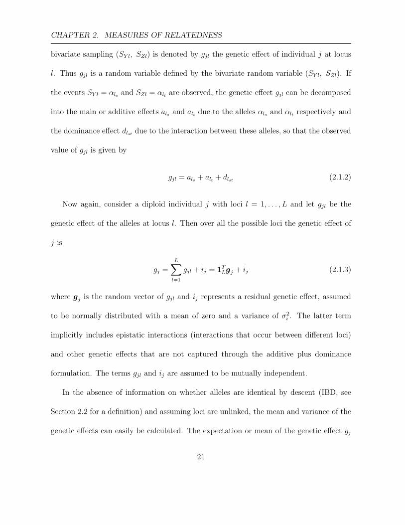
bivariate sampling (SY l, SZl) is denoted by gjl the genetic effect of individual j at locus
l. Thus gjl is a random variable defined by the bivariate random variable (SY l, SZl). If
the events SY l = αls and SZl = αlt are observed, the genetic effect gjl can be decomposed
into the main or additive effects als and alt due to the alleles αls and αlt respectively and
the dominance effect dlstdue to the interaction between these alleles, so that the observed
value of gjl is given by
gjl = als + alt + dlst(2.1.2)
Now again, consider a diploid individual j with loci l = 1, . . . , L and let gjl be the
genetic effect of the alleles at locus l. Then over all the possible loci the genetic effect of
j is
gj =
L∑
l=1
gjl + ij = 1TLgj + ij (2.1.3)
where gj is the random vector of gjl and ij represents a residual genetic effect, assumed
to be normally distributed with a mean of zero and a variance of σ2i . The latter term
implicitly includes epistatic interactions (interactions that occur between different loci)
and other genetic effects that are not captured through the additive plus dominance
formulation. The terms gjl and ij are assumed to be mutually independent.
In the absence of information on whether alleles are identical by descent (IBD, see
Section 2.2 for a definition) and assuming loci are unlinked, the mean and variance of the
genetic effects can easily be calculated. The expectation or mean of the genetic effect gj
21

CHAPTER 2. MEASURES OF RELATEDNESS
is
E(gj) = E(
L∑
l=1
gjl + ij)
=
L∑
l=1
E(gjl) + E(ij)
=L∑
l=1
nl∑
s=1
nl∑
t=1
(als + alt + dlst)plsplt + 0
=
L∑
l=1
2aTl pl + pT
l Dlpl
where aTl = (al1al2 . . . alnl
), is the vector of additive effects at locus l, pTl = (pl1pl2 . . . plnl
)
is the vector of allele probabilities at locus l and Dnl×nl
l is the matrix of dominance effects
for locus l. The weighted zero sum constraints (Eqn. 2.1.4) that are used in quantitative
genetics are applied here (and elsewhere in the derivations that follow).
nl∑
s=1
alspls = aTl pl = 0
nl∑
s=1
dlstpls = Dlpl = 0. (2.1.4)
Therefore, the expectation of the genetic effect gj is zero (i.e. E(gj) = 0). The variance
of the genetic effect gj is
var(gj) = E(g2j ) − [E(gj)]
2
= E
(
L∑
l=1
(gjl + ij)2
)
− 0
= E
(
L∑
l=1
(gjl)2
)
+L∑
l=1
E(gjlijl) + E(i2j )
22
CHAPTER 2. MEASURES OF RELATEDNESS
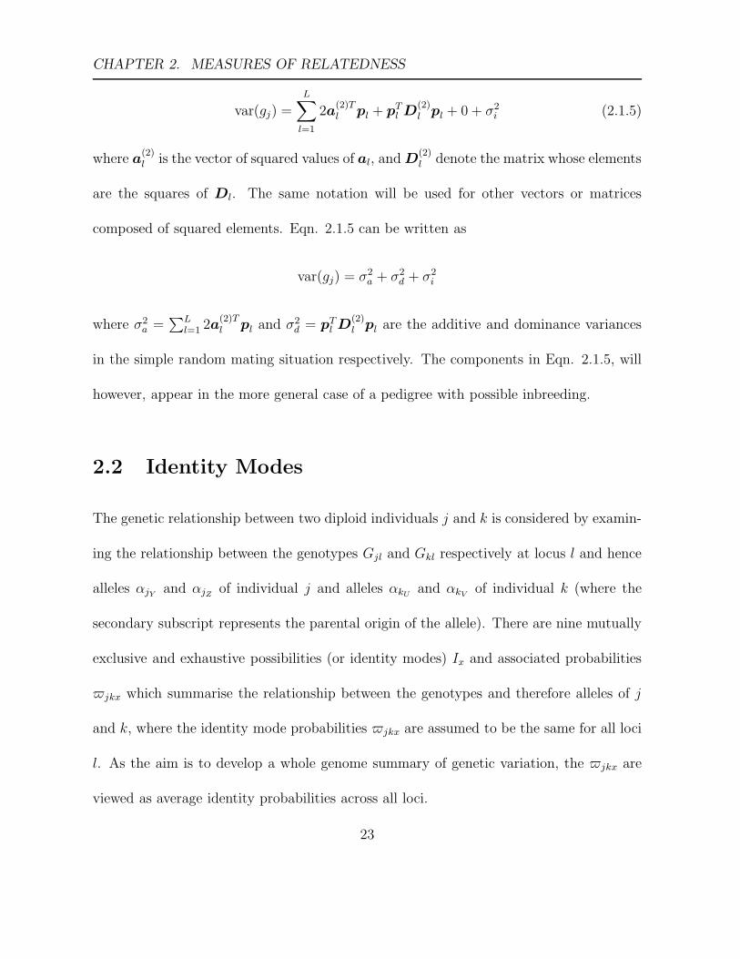
var(gj) =
L∑
l=1
2a(2)Tl pl + pT
l D(2)l pl + 0 + σ2
i (2.1.5)
where a(2)l is the vector of squared values of al, and D
(2)l denote the matrix whose elements
are the squares of Dl. The same notation will be used for other vectors or matrices
composed of squared elements. Eqn. 2.1.5 can be written as
var(gj) = σ2a + σ2
d + σ2i
where σ2a =
∑Ll=1 2a
(2)Tl pl and σ2
d = pTl D
(2)l pl are the additive and dominance variances
in the simple random mating situation respectively. The components in Eqn. 2.1.5, will
however, appear in the more general case of a pedigree with possible inbreeding.
2.2 Identity Modes
The genetic relationship between two diploid individuals j and k is considered by examin-
ing the relationship between the genotypes Gjl and Gkl respectively at locus l and hence
alleles αjYand αjZ
of individual j and alleles αkUand αkV
of individual k (where the
secondary subscript represents the parental origin of the allele). There are nine mutually
exclusive and exhaustive possibilities (or identity modes) Ix and associated probabilities
jkx which summarise the relationship between the genotypes and therefore alleles of j
and k, where the identity mode probabilities jkx are assumed to be the same for all loci
l. As the aim is to develop a whole genome summary of genetic variation, the jkx are
viewed as average identity probabilities across all loci.
23

CHAPTER 2. MEASURES OF RELATEDNESS
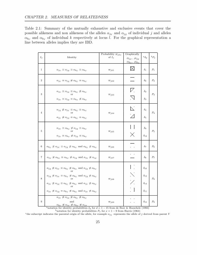
The possible identity modes are presented in Table 2.1 and are based on whether the
alleles of j are identical by descent (IBD) to the alleles of k. If alleles αls and αlt are IBD,
where this is denoted by the notation αls ≡ αlt , then the alleles are copies of the same
allele from a common ancestor. A graphical representation is also presented in Table 2.1,
where an edge between two alleles implies that these alleles are IBD and the absence of
an edge between two alleles implies that these alleles are not IBD.
The probabilities jk1 and jk2 occur when both j and k are homozygous at locus l,
jk3, jk4, jk6 and jk7 occur when one of j and k are heterozygous, and the other is
homozygous at locus l. The probabilities jk5, jk8 and jk9 occur when j and k are
both heterozygous at locus l.
24
CHAPTER 2. MEASURES OF RELATEDNESS
Table 2.1: Summary of the mutually exhaustive and exclusive events that cover thepossible alikeness and non alikeness of the alleles αjY
and αjZof individual j and alleles
αkUand αkV
of individual k respectively at locus l. For the graphical representation aline between alleles implies they are IBD.
Probability jkx GraphicallyIx Identity of Ix
aδdbPx
αkU`
`αjZ
`αkV
αjY`
1 αjY≡ αjZ
≡ αkU≡ αkV
jk1 `
`
`
`
@@�� δ1 P1
2 αjY≡ αjZ
6≡ αkU≡ αkV
jk2 `
`
`
`
δ6 P2
αjY≡ αjZ
≡ αkU6≡ αkV
`
`
`
`
�� δ23 or jk3 P3
αjY≡ αjZ
≡ αkV6≡ αkU
`
`
`
`
@@ δ3
αjZ6≡ αjY
≡ αkU≡ αkV
`
`
`
`
@@ δ44 or jk4 P4
αjY6≡ αjZ
≡ αkU≡ αkV
`
`
`
`
�� δ5
αjY≡ αkU
6≡ αjZ≡ αkV
`
`
`
`
δ95 or jk5 P5
αjY≡ αkV
6≡ αjZ≡ αkU
`
`
`
`
@@�� δ12
6 αkU6≡ αjY
≡ αjZ6≡ αkV
and αkU6≡ αkV
jk6 `
`
`
`
δ7 P6
7 αjY6≡ αkU
≡ αkV6≡ αjZ
and αjY6≡ αjZ
jk7 `
`
`
`
δ8 P7
αjZ6≡ αjY
≡ αkU6≡ αkV
and αjZ6≡ αkV
`
`
`
`
δ10or
αjZ6≡ αjY
≡ αkV6≡ αkU
and αjZ6≡ αkU
`
`
`
`
@@ δ138 or jk8 P8
αjY6≡ αjZ
≡ αkU6≡ αkV
and αjY6≡ αkV
`
`
`
`
�� δ14or
αjY6≡ αjZ
≡ αkV6≡ αkU
and αjY6≡ αkU
`
`
`
`
δ11
αjY6≡ αjZ
6≡ αkU6≡ αkV
9 and jk9 `
`
`
`
δ15 P9
αkU6≡ αjY
6≡ αkV6≡ αjZ
anotation for identity probabilities δd for d = 1 − 15 from de Boer & Hoeschele (1993)bnotation for identity probabilities Px for x = 1 − 9 from Harris (1964)
cthe subscript indicates the parental origin of the allele, for example αjYrepresents the allele of j derived from parent Y
25

CHAPTER 2. MEASURES OF RELATEDNESS
2.3 Coefficient of Coancestry
The Coefficient of Coancestry (fjk) (also known as the Coefficient of Kinship, Consan-
guinity or Parentage) of individuals j and k was originally defined by Malecot (1948) as
the probability that two gametes sampled at random one from each individual, carry ho-
mologous alleles that are IBD. It is an indication of the degree of relationship by descent
between potential parents. Let Sjl represent an allele randomly sampled from individual
j at locus l, with a similar definition for Skl. The coefficient of kinship between lines j
and k at locus l is defined by Cockerham & Weir (1984) as
fjkl = p(Sjl ≡ Skl) (2.3.6)
where as before ≡ is the notation that denotes IBD.
The coefficient of coancestry is used by plant breeders to determine the amount of
inbreeding that would result in progeny for a particular cross of parents, and thus enables
crosses to be planned which give the least amount of inbreeding in the progeny. The
probabilities that are relevant to calculating the coefficient of coancestry are where there
exists an IBD relationship between the alleles of j and k and therefore are jk1, jk3,
jk4, jk5 and jk8 (Table 2.1).
26

CHAPTER 2. MEASURES OF RELATEDNESS
The coefficient of coancestry is thus
fjkl =
9∑
x=1
p(IBD|Ix)jkx
= jk1 +1
2jk3 +
1
2jk4 +
1
2jk5 +
1
4jk8
= fjk (2.3.7)
since the identity mode locus probabilities are assumed to be the same at each locus.
The coefficient of coancestry between individuals j and k can also be expressed in
terms of the coefficients of the parents (Falconer & Mackay, 1996), as follows
fjkl = p(Sjl ≡ Skl)
= p ((SY l, SZl) ≡ (SUl, SV l))
=1
4(fY U + fY V + fZU + fZV ) (2.3.8)
2.4 Coefficient of Inbreeding
The Coefficient of Inbreeding (Fj) expresses the degree of inbreeding of individual j. It
was originally defined by Wright (1922) as the correlation between gametes that unite to
form an individual.
Malecot (1948) provides an alternative definition of the coefficient of inbreeding as
the probability that two alleles at a randomly sampled locus are IBD. The inbreeding
coefficient is thus defined as the probability that an individual has two copies of the
same allele which are derived from a common ancestor. The coefficient of inbreeding of
27

CHAPTER 2. MEASURES OF RELATEDNESS
individual j therefore expresses the degree of inbreeding of an individual and depends on
the amount of common ancestry in parents Y and Z. In terms of the sampling definition
it implies that the alleles that are sampled from the parents Y and Z of j are IBD and
therefore following a result given by Cockerham & Weir (1984)
Fjl = p(SY l ≡ SZl)
= fY Zl (by Eqn. 2.3.6)
= Y Z1 +1
2Y Z3 +
1
2Y Z4 +
1
2Y Z5 +
1
4Y Z8
= fY Z (2.4.9)
Thus the inbreeding coefficient of individual j is given by the coefficient of coancestry
of it’s parents i.e. Fj = fY Z .
2.5 Special Case of the coefficient of Coancestry
A special case is the coancestry of an individual with itself fjjl, and is thus the inbreeding
coefficient of the progeny that would be produced by self mating.
The coefficient of coancestry for individual j involves sampling from the alleles of j.
Thus for IBD, either both alleles are sampled and the alleles are IBD with probability
fY Z , or the same allele is sampled twice in which case they are IBD with probability 1.
28
CHAPTER 2. MEASURES OF RELATEDNESS
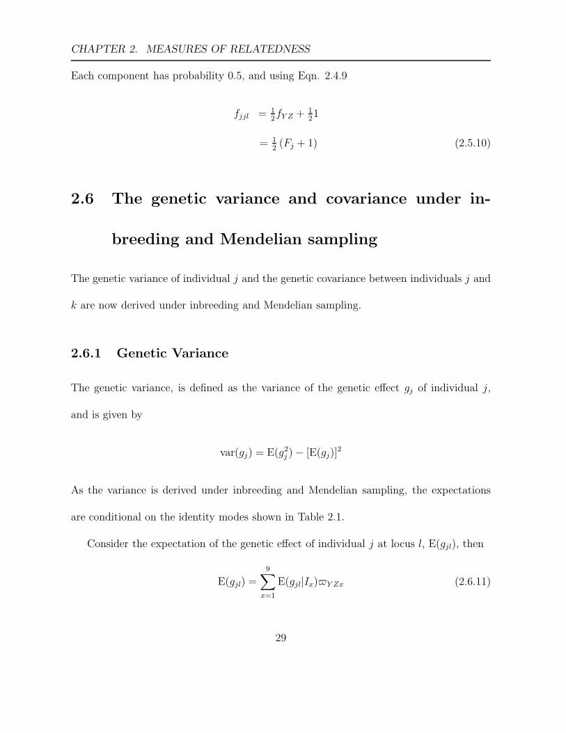
Each component has probability 0.5, and using Eqn. 2.4.9
fjjl = 12fY Z + 1
21
= 12
(Fj + 1) (2.5.10)
2.6 The genetic variance and covariance under in-
breeding and Mendelian sampling
The genetic variance of individual j and the genetic covariance between individuals j and
k are now derived under inbreeding and Mendelian sampling.
2.6.1 Genetic Variance
The genetic variance, is defined as the variance of the genetic effect gj of individual j,
and is given by
var(gj) = E(g2j ) − [E(gj)]
2
As the variance is derived under inbreeding and Mendelian sampling, the expectations
are conditional on the identity modes shown in Table 2.1.
Consider the expectation of the genetic effect of individual j at locus l, E(gjl), then
E(gjl) =9∑
x=1
E(gjl|Ix)Y Zx (2.6.11)
29

CHAPTER 2. MEASURES OF RELATEDNESS
Recall that individual j has alleles that are random samples of the alleles of it’s parents,
thus the results for E(gjl|Ix) under each identity mode Ix, given in Table 2.2 are based on
the identity probabilities Y Zx that relate to it’s parents Y and Z.
Table 2.2: Summary of the E(gjl|Ix) of individual j
Identity
Mode (Ix) E(gjl|Ix) Y Zx
I1 (2als + dlss) pls Y Z1
I2 (2als + dlss) pls Y Z2
I3 (2als + dlss) pls Y Z3
I4 (als + alt + dlst) plsplt Y Z4
I5 (als + alt + dlst) plsplt Y Z5
I6 (2als + dlss) pls Y Z6
I7 (als + alt + dlst) plsplt Y Z7
I8 (als + alt + dlst) plsplt Y Z8
I9 (als + alt + dlst) plsplt Y Z9
Assuming that j=k, the only relevant identity modes are I1 and I5 because at a locus
the alleles of an individual j are either IBD or not IBD. Thus the two relevant probabilities
are Y Z1 = Fj and Y Z5 = 1−Fj which relate to the probability that the alleles of j are
IBD or not respectively.
30

CHAPTER 2. MEASURES OF RELATEDNESS
Thus the expectation is
E(gjl) = Fjl
nl∑
s=1
(2als + dlh)pls + (1 − Fjl)
nl∑
s=1
nl∑
t=1
(als + alt + dlst)plsplt
= Fjl(2al + dlh)T pl + (1 − Fjl)pTl (al ⊗ 1T
nl+ 1nl
⊗ al + Dl)pl
= FjldTlhpl
= Fjl∆lh
= Fj∆lh (2.6.12)
where the subscript h represents two IBD alleles, ∆lh = dTlhpl and the other terms are
zero because of the constraints (Eqn. 2.1.4). If ∆h is the vector of ∆lh, then
E(gj) = Fj∆h
where gj is as defined in Eqn. 2.1.3. The mean genetic effect for line j is therefore given
by
E(gj) = Fj1TL∆h = Fj∆h (2.6.13)
Recall from Eqn. 2.1.3 that
gj =
L∑
l=1
gjl + ij = 1TLgj + ij
and therefore
g2j =
L∑
l=1
g2jl +
L∑
l1=1
l1 6=l2
L∑
l2=1
gjl1gjl2 + 2
L∑
l=1
gjlij + i2j
= 1TLgjg
Tj 1L + 21T
Lgjij + i2j (2.6.14)
31

CHAPTER 2. MEASURES OF RELATEDNESS
and hence E(g2j ) simplifies to
E(g2j ) = E(1T
LgjgTj 1L) + E(21T
Lgjij) + E(i2j )
= E(1TLgjg
Tj 1L) + σ2
i (2.6.15)
The expectation E(21TLgjij)=2E(1T
Lgj)E(ij) = 0 as these random variables are assumed
independent and E(ij) = 0. In addition E(i2j ) = σ2i . The expectation E(1T
LgjgTj 1L)
involves E(g2jl) for alleles at the same locus l and E(gjl1gjl2) for alleles at different loci l1
and l2.
Again, for an individual j there are only two relevant probabilities Y Z1 = Fj and
Y Z5 = 1− Fj, that relate to whether the alleles of j are IBD or not respectively so that
E(g2jl) =
9∑
x=1
E(g2jl|Ix)Y Zx
= Fj(2al + dlh).(2al + dlh)pl
+ (1 − Fj)pTl (al ⊗ 1T
ml+ 1ml
⊗ al + Dl).(al ⊗ 1Tml
+ 1ml⊗ al + Dl)pl
= 4Fja(2)Tl pl + Fjd
(2)Tlh pl + 4Fj(al.dlh)T pl
+ 2(1 − Fj)a(2)Tl pl + (1 − Fj)p
Tl D
(2)l pl
= 2(1 + Fj)a(2)Tl pl + (1 − Fj)p
Tl D
(2)l pl + Fjd
(2)Tlh pl + 4Fj(al.dlh)T pl
Assuming independence of loci l1 and l2,
E(gjl1gjl2) = E(gjl1)E(gjl2) = Fj∆l1hFj∆l2h
= F 2j ∆l1h∆l2h (2.6.16)
32
CHAPTER 2. MEASURES OF RELATEDNESS
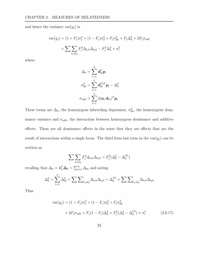
and hence the variance var(gj) is
var(gj) = (1 + Fj)σ2a + (1 − Fj)σ
2d + Fjσ
2dh + Fj∆
2h + 2Fjσadh
+∑∑
l1 6=l2
F 2j ∆l1h∆l2h − F 2
j ∆2h + σ2
i
where
∆h =L∑
l=1
dTlhpl
σ2dh =
L∑
l=1
d(2)Tlh pl − ∆2
h
σadh =L∑
l=1
2(al.dlh)T pl
These terms are ∆h, the homozygous inbreeding depression, σ2dh, the homozygous dom-
inance variance and σadh, the interaction between homozygous dominance and additive
effects. These are all dominance effects in the sense that they are effects that are the
result of interactions within a single locus. The third from last term in the var(gj) can be
written as
∑∑
l1 6=l2
F 2j ∆l1h∆l2h = F 2
j (∆2h − ∆
(2)h )
recalling that ∆h = 1TL∆h =
∑Ll=1 ∆lh and noting
∆2h =
L∑
l=1
∆2lh +
∑∑
l1 6=l2∆l1h∆l2h = ∆
(2)h +
∑∑
l1 6=l2∆l1h∆l2h
Thus
var(gj) = (1 + Fj)σ2a + (1 − Fj)σ
2d + Fjσ
2dh
+ 2Fjσadh + Fj(1 − Fj)∆2h + F 2
j (∆2h − ∆
(2)h ) + σ2
i (2.6.17)
33
CHAPTER 2. MEASURES OF RELATEDNESS
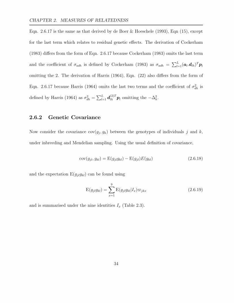
Eqn. 2.6.17 is the same as that derived by de Boer & Hoeschele (1993), Eqn (15), except
for the last term which relates to residual genetic effects. The derivation of Cockerham
(1983) differs from the form of Eqn. 2.6.17 because Cockerham (1983) omits the last term
and the coefficient of σadh is defined by Cockerham (1983) as σadh =∑L
l=1(al.dlh)T pl
omitting the 2. The derivation of Harris (1964), Eqn. (22) also differs from the form of
Eqn. 2.6.17 because Harris (1964) omits the last two terms and the coefficient of σ2dh is
defined by Harris (1964) as σ2dh =
∑Ll=1 d
(2)Tlh pl omitting the −∆2
h.
2.6.2 Genetic Covariance
Now consider the covariance cov(gj , gk) between the genotypes of individuals j and k,
under inbreeding and Mendelian sampling. Using the usual definition of covariance,
cov(gjl, gkl) = E(gjlgkl) − E(gjl)E(gkl) (2.6.18)
and the expectation E(gjlgkl) can be found using
E(gjlgkl) =9∑
x=1
E(gjlgkl|Ix)jkx (2.6.19)
and is summarised under the nine identities Ix (Table 2.3).
34
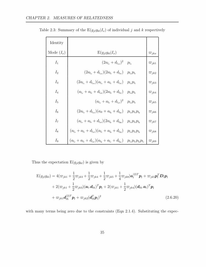
CHAPTER 2. MEASURES OF RELATEDNESS
Table 2.3: Summary of the E(gjlgkl|Ix) of individual j and k respectively
Identity
Mode (Ix) E(gjlgkl|Ix) jkx
I1 (2als + dlss)2 pls jk1
I2 (2als + dlss)(2alt + dltt) plsplt jk2
I3 (2als + dlss)(als + alt + dlst
) plsplt jk3
I4 (als + alt + dlst)(2alt + dltt) plsplt jk4
I5 (als + alt + dlst)2 plsplt jk5
I6 (2als + dlss)(alt + alb + dlbt
) plspltplb jk6
I7 (als + alt + dlst)(2alb + dlbb
) plspltplb jk7
I8 (als + alt + dlst)(alt + alb + dltb) plspltplb jk8
I9 (als + alt + dlst)(alb + alc + dlbc
) plspltplbplc jk9
Thus the expectation E(gjlgkl) is given by
E(gjlgkl) = 4(jk1 +1
2jk3 +
1
2jk4 +
1
2jk5 +
1
4jk8)a
(2)Tl pl +jk5p
Tl Dlpl
+ 2(jk1 +1
2jk3)(al.dlh)T pl + 2(jk1 +
1
2jk4)(dlh.al)
T pl
+jk1d(2)Tlh pl +jk2(d
Tlhpl)
2 (2.6.20)
with many terms being zero due to the constraints (Eqn 2.1.4). Substituting the expec-
35

CHAPTER 2. MEASURES OF RELATEDNESS
tation E(gjlgkl) and the expectation E(gjl) into Eqn. 2.6.18
cov(gjl, gkl) = 2fjk2a(2)Tl pl +jk5p
Tl Dlpl
+ 2(jk1 +1
23r)(al.dlh)T pl + 2(jk1 +
1
2jk4)(dlh.al)
T pl
+jk1d(2)Tlh pl + (jk2 − FjlFkl)(d
Tlhpl)
2 (2.6.21)
Thus the covariance cov(gj , gk), across all the loci is
cov(gj, gk) = 2fjkσ2a +jk5σ
2d + (2jk1 +
1
2(jk3 +jk4))σadh
+jk1σ2dh + (jk1 +jk2 − FjFk)∆2
h (2.6.22)
Eqn. 2.6.22 is given by Harris (1964), Eqn. (26).
2.7 Full Variance-Covariance matrix
Combining 2.6.17 and 2.6.22 the full covariance-variance matrix G of the vector of genetic
effects g = (g1g2 . . . gm)T for m individuals is given by
var(g) = G = σ2aA + σ2
dD + σadhT + σ2dhDh + (∆2
h − ∆(2)h )E + ∆2
hDI + σ2i I (2.7.23)
where A is the additive relationship matrix, D is the heterozygous dominance relationship
matrix, T is the homozygous dominance and additive covariance relationship matrix, Dh
and E are the homozygous dominance relationship matrices across the same and different
loci respectively, DI is the homozygous inbreeding depression relationship matrix and I
is the identity matrix.
36
CHAPTER 2. MEASURES OF RELATEDNESS
The Eqn. 2.7.23 is of the same form as de Boer & Hoeschele (1993) except a term for
residual genetic effects is included.
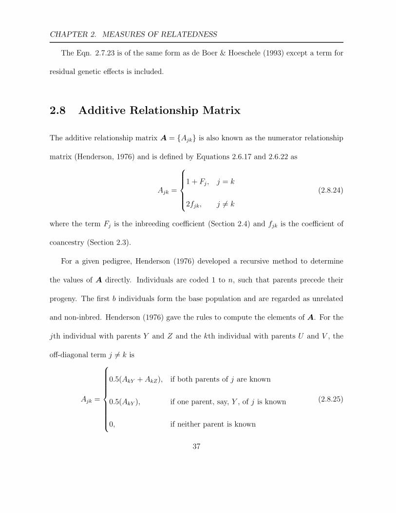
2.8 Additive Relationship Matrix
The additive relationship matrix A = {Ajk} is also known as the numerator relationship
matrix (Henderson, 1976) and is defined by Equations 2.6.17 and 2.6.22 as
Ajk =
1 + Fj , j = k
2fjk, j 6= k
(2.8.24)
where the term Fj is the inbreeding coefficient (Section 2.4) and fjk is the coefficient of
coancestry (Section 2.3).
For a given pedigree, Henderson (1976) developed a recursive method to determine
the values of A directly. Individuals are coded 1 to n, such that parents precede their
progeny. The first b individuals form the base population and are regarded as unrelated
and non-inbred. Henderson (1976) gave the rules to compute the elements of A. For the
jth individual with parents Y and Z and the kth individual with parents U and V , the
off-diagonal term j 6= k is
Ajk =
0.5(AkY + AkZ), if both parents of j are known
0.5(AkY ), if one parent, say, Y , of j is known
0, if neither parent is known
(2.8.25)
37

CHAPTER 2. MEASURES OF RELATEDNESS
the diagonal term j = k is
Ajj =
1 + 0.5AY Z , if both parents are known
1, if one or neither parents are known
(2.8.26)
2.8.1 Adjustment for self-fertilization
The work of this section was presented in Oakey et al. (2006). In plant breeding, the
test lines that are included in trials are often the result of an F5 or F6 cross, which is the
equivalent to 5 or 6 generations of self-fertilization. The method of Henderson (1976) was
developed for use in animal pedigrees, and as such requires for any particular line that
is a result of n generations of self-fertilization, that all the previous n− 1 generations of
lines involved in it’s development are included in the pedigree. Clearly, in plant breeding
trials where each test line has undergone the self-fertilization process up to n times, this
would require an (unnecessarily) large pedigree to be recorded in order to obtain an
accurate estimates of A. A modification in the calculation of the inbreeding coefficient
Fj and therefore in the Ajj value, can be incorporated into the algorithm, so that it is
unnecessary to include the n − 1 generation of lines in the pedigree, just the number of
generations n of self-fertilization need be recorded for each line. The derivation of the
adjustment is as follows:
Under self-fertilization, the Fj in the nth generation denoted here as Fj(n) is given by
38

CHAPTER 2. MEASURES OF RELATEDNESS
Falconer & Mackay (1996) as:
Fj(n) = 0.5(1 + Fj(n−1))
The diagonal Ajj value is given by
Ajj = 1 + Fj
If both parents, Y and Z of individual j are known then, for a F1 generation (not self-
fertilized) individual, the Fj(1) denoted here as Fj is given by:
Fj = Ajj − 1
= (1 + 0.5AY Z) − 1
Fj = 0.5AY Z (2.8.27)
By repeated substitution, the inbreeding coefficient in the nth generation Fj(n) can be
shown to equal
Fj(2) = 0.5(1 + 0.5AY Z)
= 0.5 + 0.52AY Z
Fj(3) = 0.5(1 + 0.5 + 0.52AY Z)
= 0.5 + 0.52 + 0.53AY Z
= 0.5(1 + 0.5) + 0.53AY Z
Fj(n) = 1 − 0.5n−1 + 0.5nAY Z
39
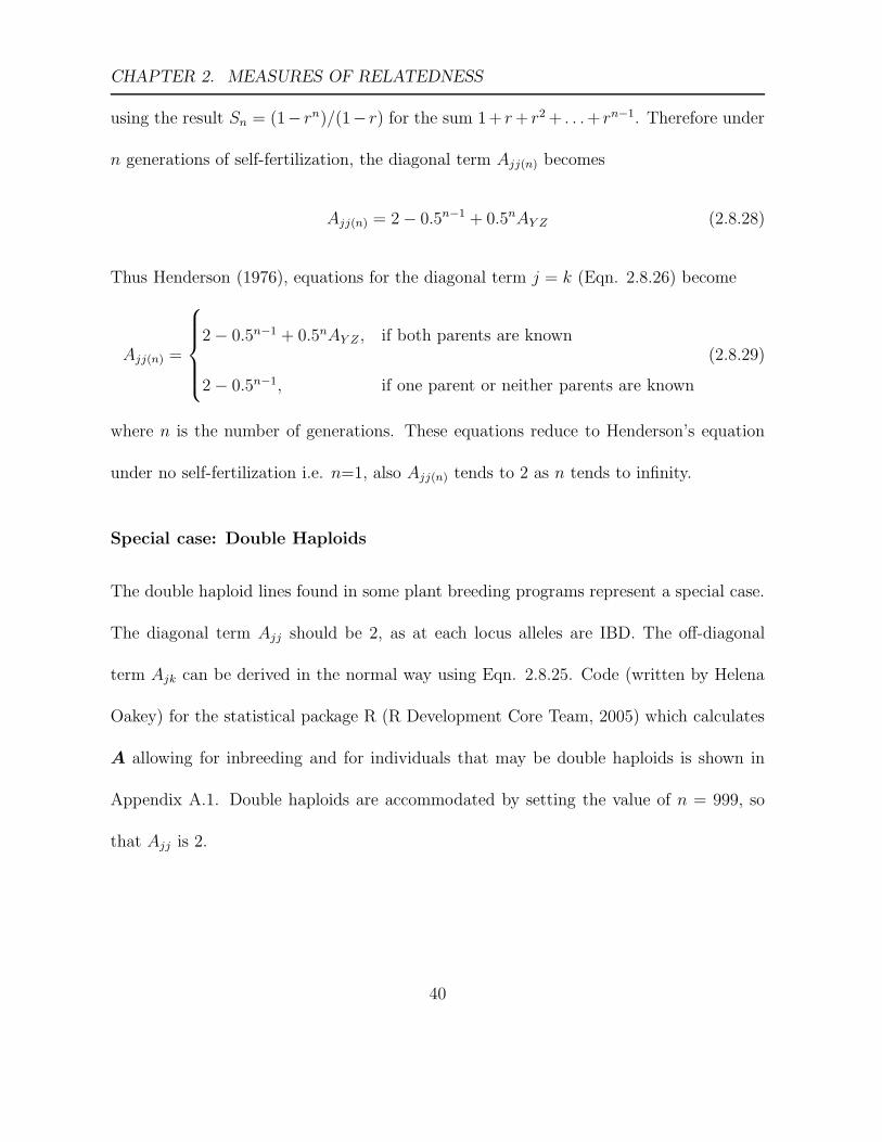
CHAPTER 2. MEASURES OF RELATEDNESS
using the result Sn = (1− rn)/(1− r) for the sum 1 + r+ r2 + . . .+ rn−1. Therefore under
n generations of self-fertilization, the diagonal term Ajj(n) becomes
Ajj(n) = 2 − 0.5n−1 + 0.5nAY Z (2.8.28)
Thus Henderson (1976), equations for the diagonal term j = k (Eqn. 2.8.26) become
Ajj(n) =
2 − 0.5n−1 + 0.5nAY Z , if both parents are known
2 − 0.5n−1, if one parent or neither parents are known
(2.8.29)
where n is the number of generations. These equations reduce to Henderson’s equation
under no self-fertilization i.e. n=1, also Ajj(n) tends to 2 as n tends to infinity.
Special case: Double Haploids
The double haploid lines found in some plant breeding programs represent a special case.
The diagonal term Ajj should be 2, as at each locus alleles are IBD. The off-diagonal
term Ajk can be derived in the normal way using Eqn. 2.8.25. Code (written by Helena
Oakey) for the statistical package R (R Development Core Team, 2005) which calculates
A allowing for inbreeding and for individuals that may be double haploids is shown in
Appendix A.1. Double haploids are accommodated by setting the value of n = 999, so
that Ajj is 2.
40

CHAPTER 2. MEASURES OF RELATEDNESS
2.8.2 The coefficient of parentage matrix-adjustment for self-
fertilization
The work of this section was presented in Oakey et al. (2006). Sneller (1994) developed an
algorithm to determine the coefficient of parentage matrix P = 0.5A, which does not take
into consideration self-fertilization. A modification in the calculation of the inbreeding
coefficient Fj and therefore fjj is necessary when dealing with individuals that have been
self-fertilized for n generations.
The coefficient of parentage fjj, for a 1st generation (ie. not self-fertilized) individual
j, with both parents Y and Z known is given by Eqn. 2.5.10:
fjj = 0.5(1 + Fj)
Under self-fertilization, the coefficient of parentage fjj(n) of j in the nth generation is
therefore given by half Equation 2.8.28 as follows:
fjj(n) = 0.5(2 − 0.5n−1 + 0.5nAY Z)
= 1 − 0.5n + 0.5n+1AY Z
= 1 − 0.5n + 0.5nfY Z since AY Z = 2fY Z
= 1 − 0.5n(1 − fY Z) (2.8.30)
Under n generations of self-fertilization, when one parent is known or when no parents
are known the value of fjj(n) is
fjj(n) = 1 − 0.5n
41

CHAPTER 2. MEASURES OF RELATEDNESS
2.9 Dominance relationship matrix
The dominance relationship between two individuals j and k results from identity state
I5 (Table 2.1). It represents the probability that the two alleles of individual j at locus
l are identical by descent (IBD) to the two alleles of individual k at the same locus and
that these two alleles are not IBD to each other.
The dominance relationship matrix D = {Djk}, has diagonal terms given by Djj =
1−Fj (Eqn. 2.6.17). However, no explicit term for the off-diagonal terms under inbreeding
has been derived.
Smith & Maki-Tanila (1990) present a method for direct computation of the inverse
of the genetic covariance matrix of (additive and) dominance effects in a population with
inbreeding, however their method is trait dependent. de Boer & Hoeschele (1993) modify
the method of Smith & Maki-Tanila (1990) and present an algorithm to determine the
relationship matrices including the dominance relationship matrix directly from a known
pedigree, where the pedigree consists of individuals and their parents.
The de Boer & Hoeschele (1993) algorithm for determining the dominance matrix from
a known pedigree consists of two main parts. The first part of the algorithm is concerned
with forming gamete pairs and includes two steps. Firstly, each parent of each individual
is allocated a gamete, so that each individual in the pedigree is defined by a unique gamete
pair. All ancestral gamete pairs for the pedigree of interest are then determined. In the
second part of the algorithm, the dominance relationship between all the possible gamete
42

CHAPTER 2. MEASURES OF RELATEDNESS
pairs (including ancestral gamete pairs) is determined. The dominance matrix is formed
from a subset of these dominance relationships which consists only of the relationships
between the gamete pairs that correspond to individuals in the pedigree.
The algorithm of de Boer & Hoeschele (1993) is most easily illustrated with an example
taken from that paper. Consider the pedigree shown in Figure 2.1 which has 4 individuals
A, B, C and D.
Figure 2.1: Example Pedigree.
The pedigree corresponding to Figure 2.1 is written in tabular form in Table 2.4. The
individuals are ordered such that parents precede offspring. Unknown parents are denoted
by zero.
Table 2.4: Pedigree of Example
Individual Parent 1 Parent 2A 0 0B A 0C A BD A B
43
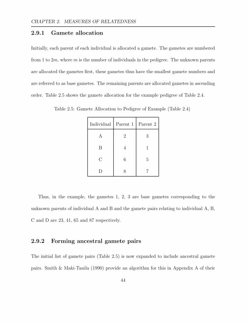
CHAPTER 2. MEASURES OF RELATEDNESS
2.9.1 Gamete allocation
Initially, each parent of each individual is allocated a gamete. The gametes are numbered
from 1 to 2m, where m is the number of individuals in the pedigree. The unknown parents
are allocated the gametes first, these gametes thus have the smallest gamete numbers and
are referred to as base gametes. The remaining parents are allocated gametes in ascending
order. Table 2.5 shows the gamete allocation for the example pedigree of Table 2.4.
Table 2.5: Gamete Allocation to Pedigree of Example (Table 2.4)
Individual Parent 1 Parent 2
A 2 3
B 4 1
C 6 5
D 8 7
Thus, in the example, the gametes 1, 2, 3 are base gametes corresponding to the
unknown parents of individual A and B and the gamete pairs relating to individual A, B,
C and D are 23, 41, 65 and 87 respectively.
2.9.2 Forming ancestral gamete pairs
The initial list of gamete pairs (Table 2.5) is now expanded to include ancestral gamete
pairs. Smith & Maki-Tanila (1990) provide an algorithm for this in Appendix A of their
44

CHAPTER 2. MEASURES OF RELATEDNESS
paper. The algorithm proceeds as follows. First a table of gamete inheritance is formed
for each gamete allocated, so that the pedigree of each gamete is written in terms of
immediate parental gametes. Table 2.6 shows the gamete inheritance for the example
pedigree of Table 2.4.
Table 2.6: Gamete Inheritance
Gamete Parent 1 Parent 2
Gamete Gamete
1 0 0
2 0 0
3 0 0
4 2 3
5 4 1
6 2 3
7 4 1
8 2 3
Notice, for example that Gamete 8 was inherited from individual A (Table 2.4). Ga-
mete 8 therefore has parental gametes corresponding to the parental gametes of individual
A which are gametes 2 and 3 (Table 2.5). The algorithm proceeds by determining ances-
tral gamete pairs. The Smith & Maki-Tanila (1990) algorithm for determining ancestral
45
CHAPTER 2. MEASURES OF RELATEDNESS
gamete pairs, starts with the four gamete pairs of individuals in the pedigree (23, 41, 65
and 87). Let rs be a gamete pair, ordered such that r ≥ s, and let the parental gametes
of r be y and z, then the following rules are used to form ancestral gamete pairs of rs.
1. if r is a base gamete, then no ancestral gamete pairs are formed
2. if r is not a base gamete and
(a) r 6= s , ancestral gamete pairs are sy and sz
(b) r = s, ancestral gamete pairs are yy and zz
The algorithm starts with the highest numbered gamete pair from the last or youngest
individual in the pedigree and proceeds for all other pedigree gamete pairs, as well as for
those ancestral gamete pairs that are added.
For example, Table 2.5, shows that highest numbered gamete pair for the example
is rs=87, where gamete 8 is the highest numbered gamete of this pair. The possible
ancestral pairs relating to the gamete pair 87 are based on the gamete pairs formed by
gamete 7 with each of the parental gametes of gamete 8 and are therefore 73 and 72.
These ancestral gamete pairs are then added to the list of total gamete pairs defined by
Table 2.5. The procedure continues then for the next highest number gamete pair (now
73) and until all the possible ancestral gamete pairs are found. Table 2.7 shows the 14
possible (ordered) gamete pairs, for the example pedigree (Table 2.4). Notice from Table
2.7, gamete pair numbers 4, 6, 11 and 14 correspond to the gamete pairs of the individuals
46

CHAPTER 2. MEASURES OF RELATEDNESS
A, B, C and D respectively and the rest are ancestral gamete pairs.
Table 2.7: All possible Gamete Pairs
Gamete pair number Gamete 1 Gamete 2
1 2 1
2 2 2
3 3 1
4 3 2
5 3 3
6 4 1
7 4 2
8 4 3
9 5 2
10 5 3
11 6 5
12 7 2
13 7 3
14 8 7
47
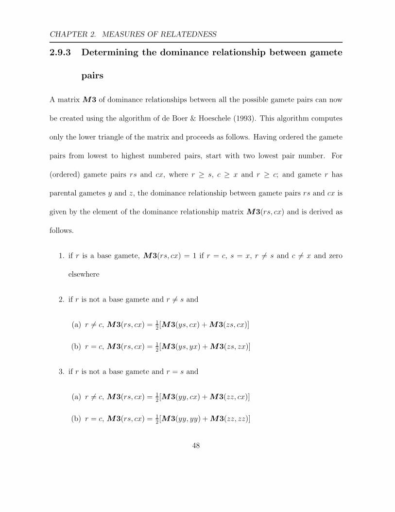
CHAPTER 2. MEASURES OF RELATEDNESS
2.9.3 Determining the dominance relationship between gamete
pairs
A matrix M3 of dominance relationships between all the possible gamete pairs can now
be created using the algorithm of de Boer & Hoeschele (1993). This algorithm computes
only the lower triangle of the matrix and proceeds as follows. Having ordered the gamete
pairs from lowest to highest numbered pairs, start with two lowest pair number. For
(ordered) gamete pairs rs and cx, where r ≥ s, c ≥ x and r ≥ c; and gamete r has
parental gametes y and z, the dominance relationship between gamete pairs rs and cx is
given by the element of the dominance relationship matrix M3(rs, cx) and is derived as
follows.
1. if r is a base gamete, M3(rs, cx) = 1 if r = c, s = x, r 6= s and c 6= x and zero
elsewhere
2. if r is not a base gamete and r 6= s and
(a) r 6= c, M3(rs, cx) = 12[M3(ys, cx) + M3(zs, cx)]
(b) r = c, M3(rs, cx) = 12[M3(ys, yx) + M3(zs, zx)]
3. if r is not a base gamete and r = s and
(a) r 6= c, M3(rs, cx) = 12[M3(yy, cx) + M3(zz, cx)]
(b) r = c, M3(rs, cx) = 12[M3(yy, yy) + M3(zz, zz)]
48

CHAPTER 2. MEASURES OF RELATEDNESS
Using Rules 1. to 3., the lower triangle of the resulting matrix M3 formed for the
example (Table 2.4) is
21 22 31 32 33 41 42 43 52 53 65 72 73 87
21 1
22 0 0
31 0 0 1
32 0 0 0 1
33 0 0 0 0 0
41 0.5 0 0.5 0 0 1
42 0 0 0 0.5 0 0 0.5
43 0 0 0 0.5 0 0 0 0.5
52 0.5 0 0 0.25 0 0.25 0.25 0 0.75
53 0 0 0.5 0.25 0 0.25 0 0.25 0 0.75
65 0.25 0 0.25 0.25 0 0.25 0.125 0.125 0.375 0.375 0.75
72 0.5 0 0 0.25 0 0.25 0.25 0 0.375 0 0.1875 0.75
73 0 0 0.5 0.25 0 0.25 0 0.25 0 0.375 0.1875 0 0.75
87 0.25 0 0.25 0.25 0 0.25 0.125 0.125 0.1875 0.1875 0.1875 0.375 0.375 0.75
The dominance relationship matrix D of individuals A, B, C and D of the example
pedigree (Table 2.4) is a subset of the matrix M3 given by the relationship between
gamete pairs 32, 41, 65, 87 and is
D =
A
B
C
D
A B C D
1 0 0.25 0.25
0 1 0.25 0.25
0.25 0.25 0.75 0.1875
0.25 0.25 0.1875 0.75
49

CHAPTER 2. MEASURES OF RELATEDNESS
2.9.4 Diagonal elements of M3
The diagonal elements of M3 can be formed separately from the off-diagonal elements.
All diagonal elements are of the form M3(rs, rs), so that r = c and s = x, r ≥ s.
1. if r is a base gamete,
M3(rs, rs) =
1, r > s
0, r = s
(2.9.31)
2. if r is not a base gamete and r > s, then
M3(rs, rs) =1
2[M3(ys, ys) + M3(zs, zs)] (2.9.32)
3. if r is not a base gamete and r = s, then
M3(rr, rr) =1
2[M3(yy, yy) + M3(zz, zz)] (2.9.33)
= 0
When r is not a base gamete, Eqn 2.9.32 implies by definition that each diagonal element
is determined using sums of diagonal elements of gamete pairs with lower order terms.
In addition, if r = s, as in Eqn 2.9.33, the result is zero. These values are always zero
because they are only ever derived from lower order terms of the same form and those
involving base gametes are by definition (Eqn. 2.9.31) zero.
50

CHAPTER 2. MEASURES OF RELATEDNESS
2.9.5 Adjustment for Self-fertilization M3
In Section 2.8.1 the adjustment for self-fertilization of the diagonal terms of the additive
relationship matrix was determined. Here the adjustment for self-fertilization for the
diagonal terms of M3 is presented.
Recall that for individual j with parents Y and Z, the diagonal term of the dominance
matrix is given by Djj = 1−Fj (Eqn. 2.6.17) and diagonal term of the additive matrix is
given by Ajj = 1 + Fj (Eqn. 2.8.24) . The diagonal dominance term Djj can be written
in terms of the additive diagonal term Ajj by using Eqn. 2.8.24
Djj = 1 − Fj
= 2 − (1 + Fj)
= 2 −Ajj (2.9.34)
or alternatively using Eqn. 2.8.27
Djj = 1 − Fj
Djj = 1 − 0.5AY Z (2.9.35)
Let individual j have gamete pair rs, then the dominance value Djj of individual j is
given by M3(rs, rs). Assuming no inbreeding and using Eqn. 2.9.34 and 2.9.35 then by
definition.
Djj = M3(rs, rs) = 2 − Ajj = 1 − 0.5AY Z (2.9.36)
51

CHAPTER 2. MEASURES OF RELATEDNESS
Recall the adjustments for inbreeding for the additive diagonal term Ajj(n) where n is
the number of generations of self-fertilization is given by Eqn.2.8.29 as
Ajj(n) =
2 − 0.5n−1 + 0.5nAY Z , if both parents are known
2 − 0.5n−1, if one parent or neither parents are known
The dominance values of the diagonal terms of M3 matrix need to be also be adjusted
to allow for self-fertilization. The two scenarios of Eqn. 2.8.29 must correspond to the
cases where either r is a base gamete or not.
Consider individual j with gamete pair rs and let individual j undergo n generations
of self-fertilization, then of interest is M3(rs, rs)(n) = Djj(n). Consider the case where r
is a base gamete, then from Eqn. 2.9.36
M3(rs, rs)(n) = 2 −Ajj(n)
= 2 − (2 − 0.5n−1)
= 0.5n−1 (2.9.37)
Now consider the case where r is not a base gamete. It is proposed that the value of
M3(rs, rs)(n) in the nth generation is
M3(rs, rs)(n) = 0.5n[M3(ys, ys) + M3(zs, zs)] (2.9.38)
This is now proved by induction. Let n=1, then
M3(rs, rs)(1) = M3(rs, rs) = 0.5[M3(ys, ys) + M3(zs, zs)] (2.9.39)
52
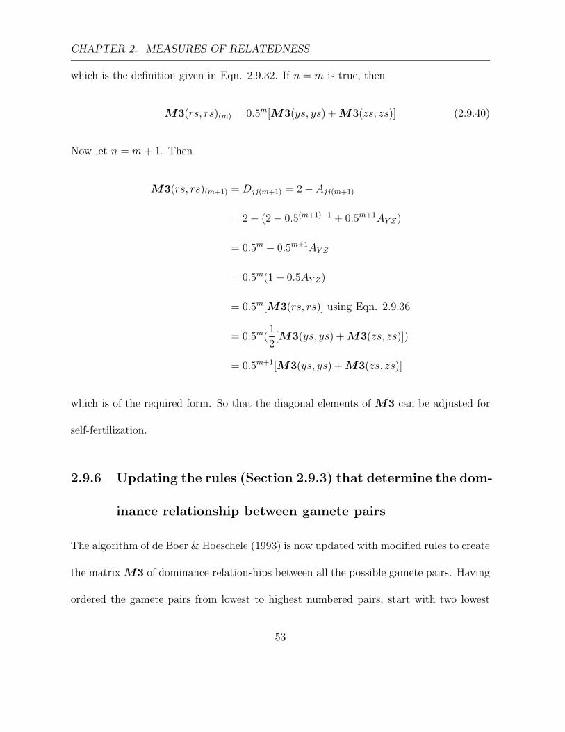
CHAPTER 2. MEASURES OF RELATEDNESS
which is the definition given in Eqn. 2.9.32. If n = m is true, then
M3(rs, rs)(m) = 0.5m[M3(ys, ys) + M3(zs, zs)] (2.9.40)
Now let n = m + 1. Then
M3(rs, rs)(m+1) = Djj(m+1) = 2 − Ajj(m+1)
= 2 − (2 − 0.5(m+1)−1 + 0.5m+1AY Z)
= 0.5m − 0.5m+1AY Z
= 0.5m(1 − 0.5AY Z)
= 0.5m[M3(rs, rs)] using Eqn. 2.9.36
= 0.5m(1
2[M3(ys, ys) + M3(zs, zs)])
= 0.5m+1[M3(ys, ys) + M3(zs, zs)]
which is of the required form. So that the diagonal elements of M3 can be adjusted for
self-fertilization.
2.9.6 Updating the rules (Section 2.9.3) that determine the dom-
inance relationship between gamete pairs
The algorithm of de Boer & Hoeschele (1993) is now updated with modified rules to create
the matrix M3 of dominance relationships between all the possible gamete pairs. Having
ordered the gamete pairs from lowest to highest numbered pairs, start with two lowest
53

CHAPTER 2. MEASURES OF RELATEDNESS
pair number. For gamete pairs rs and cx, where r ≥ s, c ≥ x and r ≥ c, let gamete
r have parental gametes y and z, let n be the number of generations of self-fertilization
for an individual j. Then, the dominance relationship between gamete pairs rs and cx
given by the element of the dominance relationship matrix M3(rs, cx) is now defined for
diagonal and off-diagonal elements as follows
Diagonal Elements of M3
All diagonal elements are of the form M3[rs, rs], so that r = c and s = x, r ≥ s.
1. if r is a base gamete
M3(rs, rs) =
0.5n−1, r > s
0, r = s
(2.9.41)
2. if r is not a base gamete and r > s, then
M3(rs, rs) = 0.5n[M3(ys, ys) + M3(zs, zs)] (2.9.42)
3. if r is not a base gamete and r = s, then
M3(rr, rr) = 0 (2.9.43)
Off-Diagonal Elements of M3
All off-diagonal elements are of the form M3[rs, cx], such that r ≥ s and excludes the
case where (r = c and s = x).
54
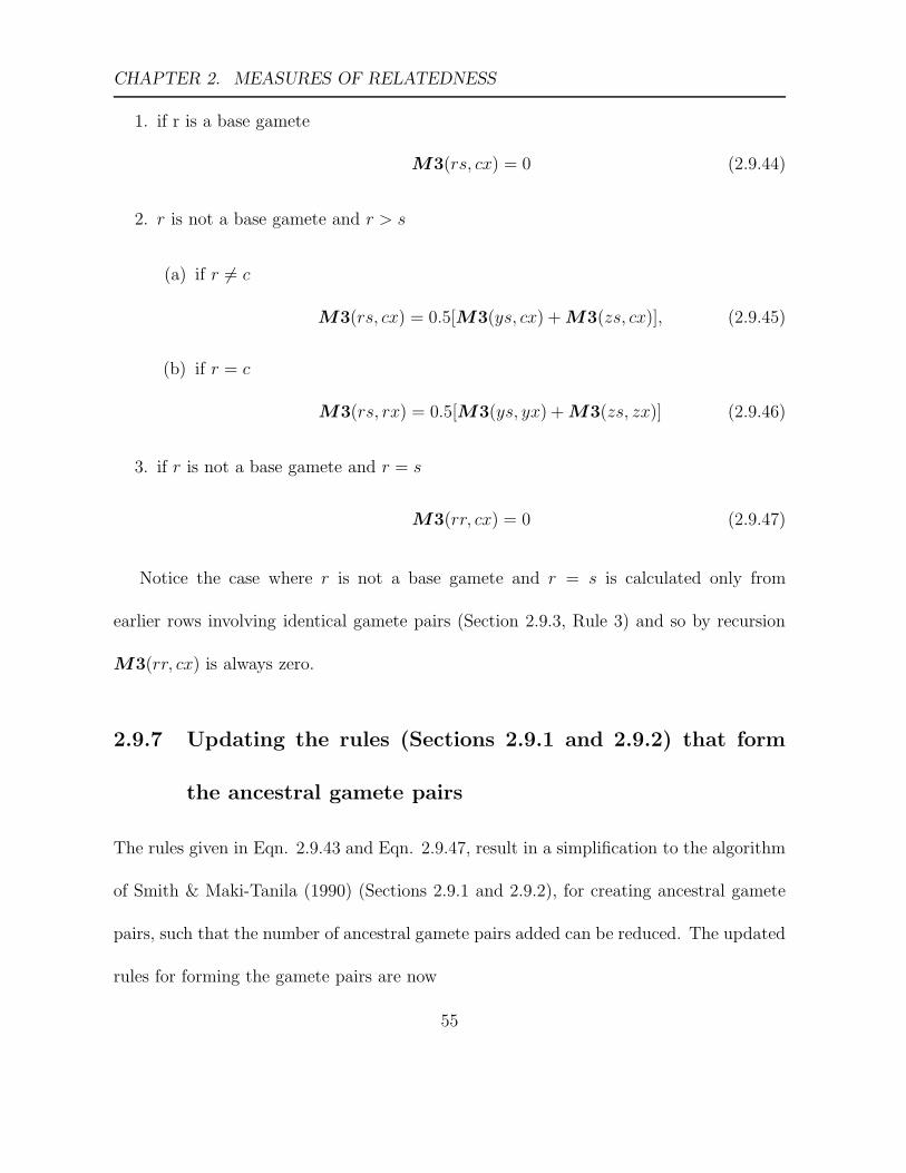
CHAPTER 2. MEASURES OF RELATEDNESS
1. if r is a base gamete
M3(rs, cx) = 0 (2.9.44)
2. r is not a base gamete and r > s
(a) if r 6= c
M3(rs, cx) = 0.5[M3(ys, cx) + M3(zs, cx)], (2.9.45)
(b) if r = c
M3(rs, rx) = 0.5[M3(ys, yx) + M3(zs, zx)] (2.9.46)
3. if r is not a base gamete and r = s
M3(rr, cx) = 0 (2.9.47)
Notice the case where r is not a base gamete and r = s is calculated only from
earlier rows involving identical gamete pairs (Section 2.9.3, Rule 3) and so by recursion
M3(rr, cx) is always zero.
2.9.7 Updating the rules (Sections 2.9.1 and 2.9.2) that form
the ancestral gamete pairs
The rules given in Eqn. 2.9.43 and Eqn. 2.9.47, result in a simplification to the algorithm
of Smith & Maki-Tanila (1990) (Sections 2.9.1 and 2.9.2), for creating ancestral gamete
pairs, such that the number of ancestral gamete pairs added can be reduced. The updated
rules for forming the gamete pairs are now
55

CHAPTER 2. MEASURES OF RELATEDNESS
1. if r is a base gamete, then no ancestral gamete pairs are formed
2. if r is not a base gamete,
(a) r 6= s , ancestral gamete pairs are sy and sz
(b) r = s, no ancestral gamete pairs are formed
To illustrate the new rules, the pedigree of Table 2.4 is expanded by the addition of
individual E with parent 1 being C and parent 2 being C. This expanded pedigree and
it’s gamete allocation is shown in Table 2.8.
Table 2.8: Pedigree and Gamete Allocation
Individual Parent 1 Parent 2 Gamete GameteParent 1 Parent 2
A 0 0 2 3B A 0 4 1C A B 6 5D A B 8 7E C C 10 9
First as an illustration of the results of the updated rules the gamete pairs formed using
the old rules given in Section 2.9.2 are examined. Here 21 gamete pairs are obtained and
are shown in Table 2.9.
56

CHAPTER 2. MEASURES OF RELATEDNESS
Table 2.9: All possible Gamete Pairs
Gamete pair number Gamete 1 Gamete 21 1 12 2 13 2 24 3 15 3 26 3 37 4 18 4 29 4 310 4 411 5 212 5 313 5 514 6 515 6 616 7 217 7 318 8 719 9 520 9 621 10 9
Notice from Table 2.9 that the gamete pairs 66 and 55 are introduced by recursion
from gamete pairs 96 and 95 respectively using Rule 2a (Section 2.9.2), also that the
gamete pairs 33 and 22 are introduced by recursion from gamete pair 66, and the gamete
pairs 44 and 11 are introduced by recursion from gamete pair 55 using Rule 2b (Section
2.9.2). Recall from the updated rules that any terms of the form M3(rr, rr) are zero
(Eqn. 2.9.43) and so these two sets of gamete pairs (33 and 22) and (44 and 11) are not
needed for the calculation of the dominance relationship of M3(66, 66) and M3(55, 55)
57
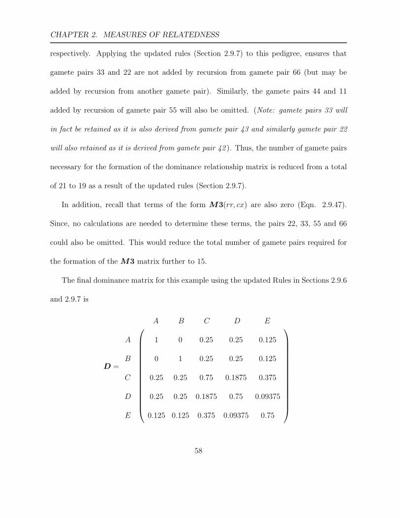
CHAPTER 2. MEASURES OF RELATEDNESS
respectively. Applying the updated rules (Section 2.9.7) to this pedigree, ensures that
gamete pairs 33 and 22 are not added by recursion from gamete pair 66 (but may be
added by recursion from another gamete pair). Similarly, the gamete pairs 44 and 11
added by recursion of gamete pair 55 will also be omitted. (Note: gamete pairs 33 will
in fact be retained as it is also derived from gamete pair 43 and similarly gamete pair 22
will also retained as it is derived from gamete pair 42 ). Thus, the number of gamete pairs
necessary for the formation of the dominance relationship matrix is reduced from a total
of 21 to 19 as a result of the updated rules (Section 2.9.7).
In addition, recall that terms of the form M3(rr, cx) are also zero (Eqn. 2.9.47).
Since, no calculations are needed to determine these terms, the pairs 22, 33, 55 and 66
could also be omitted. This would reduce the total number of gamete pairs required for
the formation of the M3 matrix further to 15.
The final dominance matrix for this example using the updated Rules in Sections 2.9.6
and 2.9.7 is
D =
A
B
C
D
E
A B C D E
1 0 0.25 0.25 0.125
0 1 0.25 0.25 0.125
0.25 0.25 0.75 0.1875 0.375
0.25 0.25 0.1875 0.75 0.09375
0.125 0.125 0.375 0.09375 0.75
58
CHAPTER 2. MEASURES OF RELATEDNESS
2.10 Special Case: The dominance relationship ma-
trix under no inbreeding
The dominance relationship is now presented for a special case: under no inbreeding. In
cases where the pedigree extends over tens of thousands of individuals it may be necessary
to assume that there is no inbreeding within the pedigree in order to make the calculation
of the dominance relationship matrix more feasible.
The dominance relationship Djk between individual j who has parents Y and Z and
individual k, who has parents U and V , under no inbreeding has been derived by Cock-
erham (1954) and its defined as
Djk =
1, j = k
0.25(AY UAZV + AY VAZU) j 6= k
(2.10.48)
where AY U is the additive relationship between individuals Y and U , and the diagonal
term of dominance relationship matrix are assumed to be one. Thus Djk is determined
from elements of the additive relationship matrix A, which has the same dimension as
the dominance relationship matrix D.
59
CHAPTER 2. MEASURES OF RELATEDNESS
2.11 A new method for calculating the dominance
relationship matrix under no inbreeding
Here an alternative method for calculating the dominance relationship matrix under no
inbreeding is presented. This method does not depend on the calculation of the additive
relationship matrix. It therefore does not require the storage of the additive relationship
values. The method has two main parts. The first part involves the allocation of gametes
to individuals in the pedigree as in the method of de Boer & Hoeschele (1993) outlined
in Section 2.9. The second part then proceeds by noting that all non-base gametes can
written in terms of base gametes. These base gametes have a probability of inheritance
associated with each individual. In this second part, these probabilities of inheritance
of the base gametes can be used to calculate the required dominance relationships. The
dominance relationship calculations therefore rely on the calculation of a matrix that has
potentially much smaller dimensions than the additive relationship matrix resulting in
gains of efficiency and storage. The dimensions of this former matrix will be at most
2m× b, where m is the number of individuals and b is the number of base gametes, where
b << m. As an example of the reduction in data points requiring storage, the pedigree in
Chapter 5 is used. This pedigree has m = 2663 individuals and A has over 3.5 million data
points (assuming just the upper triangle of A is calculated). Under the new approach,
the number of base gametes b=185 and therefore at most under 1 million data points
corresponding to gamete probabilities are required. The number of data points calculated
60
CHAPTER 2. MEASURES OF RELATEDNESS
is likely to be lower than 2m × b as just the rows which correspond to individuals that
are parents need to be calculated.
Consider the example pedigree (Table 2.4). Recall the base gametes are 1, 2 and
3. The gametes of all individuals can be written in terms of the base gametes. This
is because each individual inherits it’s gametes from it’s parents and therefore the only
gametes that an individual can inherit are those that are carried by it’s parents. Thus,
parental gametes are passed on to their offspring with an associated probability that can
be determined. These parental gametes must take the form of the base gametes because
of the rules of inheritance. Consider again the example pedigree, parent 1 of B is A. Thus
B will have inherited gamete 1 or 2 from A with probability 0.5 and gamete 3 (a base
gamete) from it’s unknown parent with probability 1. So the possible gamete pairs of
B are the possible combinations of gametes from parent 1 and parent 2 and thus are 13
or 23, each of which occurs with probability (1 × 0.5). Individual B will pass on to it’s
offspring, either gametes 1 or 2 with probability 0.25 or gamete 3 with probability 0.5.
The inheritance of base gametes for all individuals in the example pedigree is shown in
Table 2.10. This inheritance of base gametes forms the basis of the algorithm which is
now presented.
61

CHAPTER 2. MEASURES OF RELATEDNESS
Table 2.10: Inheritance of Base Gamete
Individual Parent 1 Parent 2
A 1 2
B 1, 2 3
C 1, 2 1, 2, 3
D 1, 2 1, 2, 3
2.11.1 Gamete Allocation
This is the same as the gamete allocation in the Smith & Maki-Tanila (1990) algorithm
(Section 2.9.1), so that each parent of each individual is allocated a gamete. The base
gametes need to be noted.
2.11.2 The probability of the inheritance of gametes
Each individual’s gametes can be expressed in terms of the base gametes as illustrated in
Table 2.10. The probability of inheritance of the base gametes will generally be different in
each individual (unless they have the same parents). A table containing the probabilities
of each base gamete for each parent of each individual can be created. Each individual will
be represented by two rows of probabilities for base gametes, one corresponding to each
of it’s parent. Each column in the table of probability will correspond to a base gamete.
62

CHAPTER 2. MEASURES OF RELATEDNESS
The rules for forming the table of probabilities are as follows. For each individual, each
of the gametes – paternal (parent 1 say) and maternal (parent 2 say) allocated (see Table
2.5 for example pedigree), are examined in turn and a corresponding row for each in the
table of probabilities is determined as follows.
1. if the gamete is a base gamete (i.e. examining the pedigree (Table 2.4) shows the
parent has value zero) then this base gamete takes probability 1 and the other base
gametes have value zero.
2. if the gamete is not a base gamete (i.e. examining the pedigree (Table 2.4) indicates
a parent P say) then the value of the probability of this gamete in terms of base
gametes is 0.5(pm + pf) where the pm corresponds to the paternal parent row of
probabilities and pf corresponds to the maternal parent row of probabilities.
This table of probabilities has all the information needed to calculate dominance of each
individual and each pair of individuals. For the example pedigree, Table 2.11 shows the
probabilities of base gametes for each individual.
63

CHAPTER 2. MEASURES OF RELATEDNESS
Table 2.11: Table of probabilities for the base gamete
Base gamete
Individual Parent 1 2 3 Comment
A m 1 0 0 base gamete
f 0 1 0 base gamete
B m 0.5 0.5 0 0.5(aTm + aT
f )
f 0 0 1 base gamete
C m 0.5 0.5 0 0.5(aTm + aT
f )
f 0.25 0.25 0.5 0.5(bTm + bT
f )
D m 0.5 0.5 0 0.5(aTm + aT
f )
f 0.25 0.25 0.5 0.5(bTm + bT
f )
athe rows of individual C and D have been included for illustration only – they are not required for the
calculation of D because C and D are not parents.
2.11.3 Calculating dominance relationships
The calculation of the dominance relationships is straightforward. Let each row of the
table of probabilities be considered a vector, for example let the probabilities of the base
gametes for paternal parent (parent 1 say) of individual j be jTm and for maternal parent
(parent 2 say) be jTf . Then the diagonal elements Djj of D the dominance relationship
matrix are the probabilities that the individual is not inbred (i.e. has different base
64

CHAPTER 2. MEASURES OF RELATEDNESS
gametes) and are given by
Djj = 1 − jmjTf (2.11.49)
The second part of Eqn. 2.11.49 is the probability that individual j inherits the same
base alleles from both parents and thus is inbred. Notice that this calculation assumes
that parents of j are not inbred. However, it is possible to get values of less than one if
the parents are not inbred but they both have a probability of sharing at least one base
gamete. If one or both parents are unknown then Djj = 1 by definition.
The off-diagonal elements Djk of D the dominance relationship matrix are the prob-
abilities that individuals j and k are both not inbred and both have same gamete pair
(for example j might have gamete pair 12 and k may have gamete pair 12). Then Djk
the dominance relationship between individual j and k is given by
Djk = sum(
(jTmjf ).(kT
mkf ))
+ sum(
(jTf jm).(kT
mkf))
− 2(
diag(jTmjf)(diag(kT
mkf))T)
(2.11.50)
where . indicates the Hadamard product of the two matrices and diag() indicates take the
diagonal elements of the matrix. Notice that here jTmjf gives the matrix of probabilities
of each possible gamete pair of j and therefore for example the first term is the sum of
the probabilities that j and k have the same gamete pair. Also notice that gamete pair
12 is not equivalent to gamete pair 21, which is the purpose of the second sum. The third
sum removes the cases where the gamete pair contains two copies of the same gamete and
65

CHAPTER 2. MEASURES OF RELATEDNESS
are thus inbred. Consider again the example pedigree,
DAA = 1 − (1 0 0)(0 0 1)T
= 1
DAC = sum
1
0
0
(
0 1 0
)
.
0.5
0.5
0
(
0.25 0.25 0.5
)
+sum
0
1
0
(
1 0 0
)
.
0.5
0.5
0
(
0.25 0.25 0.5
)
−2
diag
1
0
0
(
0 1 0
)
diag
0.5
0.5
0
(
0.25 0.25 0.5
)
T
= sum
0 1 0
0 0 0
0 0 0
.
0.125 0.125 0.25
0.125 0.125 0.25
0 0 0
+sum
0 0 0
1 0 0
0 0 0
.
0.125 0.125 0.25
0.125 0.125 0.25
0 0 0
− 2(0 0 0)(0.125 0.125 0)T
66
CHAPTER 2. MEASURES OF RELATEDNESS
= 0.125 + 0.125 − 0
DAC = 0.25
2.12 Inverse of the Relationship Matrices
The inverses of the relationship matrices are required for the mixed model equations (see
Henderson, 1984). Thus the size of the matrices may be a limiting factor in calculating
the inverse directly using conventional rules for inverting matrices. There are several
algorithms (Henderson, 1976, Quaas, 1976 and Meuwissen & Luo, 1992) for the direct
calculation of the inverse of the additive relationship matrix and therefore no obstacles
to fitting this term. However, there is no algorithm to calculate the inverses of the other
matrices given in Eqn. 2.7.23 directly. Therefore, for large pedigrees obtaining the inverse
of these relationship matrices may be a limiting factor to the fitting of these effects.
2.12.1 Inverse of the Additive Relationship Matrix
The algorithm used by ASReml (Gilmour et al., 2006) to compute the inverse of the addi-
tive relationship matrix A−1 will be presented. ASReml uses an approach to computing
A−1 that is a modification of the approach presented by Meuwissen & Luo (1992). It
computes A and A−1 line by line, by adding the relationship of a single individual at
a time and thus requires both A and A−1 to be retained in the staged process. As a
precursor to the algorithm, consider the matrix K which can be written in partitioned
67

CHAPTER 2. MEASURES OF RELATEDNESS
form as
K =
K11 k12
kT12 k22
Thus a single row and column have been added to the matrix K11, to form K, where k12
is a vector and k22 is a scalar.
The inverse of K is given by
K−1 =
K−111 + K−1
11 k12k22kT
12K−111 −K−1
11 k12k22
−k22kT12K
−111 k22
(2.12.51)
where
k22 = (k22 − kT12K
−111 k12)−1
Thus the inverse of K can be found using the inverse of K11.
In this way by progressively adding a single row and column to K and it’s inverse K−1
the full matrices can be obtained. Now the additive relationship matrix and it’s inverse
will be considered. Consider first a partially complete additive relationship matrix A1. If
the relationships with individual j which has parents Y and Z are to be added to A1 to
form an updated additive relationship matrix A2, then
A2 =
A1 A1pY Z
pTY ZA1 2 − 0.5n−1 + 0.5nAY Z
(2.12.52)
Notice that if the matrix A1 is formed from individuals who consists only from the base
population (i.e. individuals with unknown parents) then A1 = I, the identity matrix.
Equating the elements of A2 to the elements of K, then K11 = A1, k12 = A1pY Z ,
68

CHAPTER 2. MEASURES OF RELATEDNESS
where pY Z is a vector which averages the parental rows of j, thus it has zeros everywhere
except the positions that correspond to parents Y and Z, where it has 0.5 and k22 =
2 − 0.5n−1 + 0.5nAY Z (Eqn. 2.8.28), where AY Z is the additive relationship between
individuals Y and Z. Thus A is built up recursively.
Now consider the inverse of the partitioned matrix A2. Using Eqn. 2.12.51, the form
of A−12 is
A−12 =
A−11 + A−1
1 A1pY Zk22pT
Y ZA1A−11 A−1
1 A1pY Zk22
k22pTY ZA1A
−11 k22
(2.12.53)
This simplifies to
A−12 =
A−11 + k22pY ZpT
Y Z k22pY Z
k22pTY Z k22
(2.12.54)
where
k22 = (2 − 0.5n−1 + 0.5nAY Z − pTY ZA1A
−11 A1pY Z)−1
= 1/{2 − 0.5n−1 + 0.5nAY Z − 0.5AY Z −1
4(AY Y + AZZ)}
Thus the update to the inverse is very simple computationally. k22 can be written
more compactly as
k22 = 1/{1 + (1 − 0.5n−1) + 0.5AY Z(0.5n−1 − 1) −1
4(AY Y + AZZ)}
= 1/{1 + (1 − 0.5n−1)(1 − 0.5AY Z) −1
4(AY Y + AZZ)} (2.12.55)
69

CHAPTER 2. MEASURES OF RELATEDNESS
Thus, it should be noted that when n >1, A1 is needed to evaluate AY Z . However, when
n = 1, k22 simplifies to
k22 = 1/{1 −1
4(AY Y + AZZ)}
so that only the diagonal terms of A are required.
70

Chapter 3
Modern approaches for the analysis
of field trials
An overview of current and appropriate or Standard statistical models for the analysis
of multi-environment field trials is presented in this chapter. These models are then ex-
tended so that the selection of best performing lines, best parents, and best combination
of parents can be determined. The extension involves partitioning the genetic line ef-
fects into additive, dominance and residual non-additive effects. The dominance effects
are estimated through the incorporation of the dominance relationship matrix. A com-
putationally efficient way of fitting dominance effects is presented in which dominance
effects are partitioned into between family dominance and within family dominance line
effects. The overall approach is applicable to inbred lines, hybrid lines and other popula-
71

CHAPTER 3. MODERN APPROACHES FOR THE ANALYSIS OF FIELD TRIALS
tion structures where pedigree information is available. Lastly, a generalized definition of
heritability is developed to account for the complex models presented in this Chapter.
3.1 Standard Statistical Model
Both single field trial and multi-environment trial analyses can be summarised by the
baseline model
y = Zgγ + ε (3.1.1)
where y(n×1) is the full vector of responses data of individual plots across each of p
environments (synonymous with trials), γ(mp×1) = (γT1 , . . . ,γ
Tp )T where γT
t is the (m×1)
subvector of genetic line means in the tth environment, the associated design matrix
Z(n×mp)g , relates plots to environment by line combinations, ε(n×1) = (εT
1 , . . . , εTp )T has εT
t
as the (nt×1) subvector of residual effects in environment t, with n =∑p
t=1 nt, where nt is
the number of observations in the tth environment. Note: here and elsewhere environment
is synonymous with site and trial
Thus the genetic line means γ reflect the genetic variation and ε provides the under-
lying structure for non-genetic variation of the response y.
The most modern methods of mixed model analysis currently in use will now be
summarized by considering appropriate models for γ and ǫ.
72

CHAPTER 3. MODERN APPROACHES FOR THE ANALYSIS OF FIELD TRIALS
3.1.1 Models for the non-genetic effects
Non-genetic effects occur at the environmental level and should include model based terms
that allow for spatial trends and randomisation based terms which are determined from
the experimental design. The approach of Gilmour et al. (1997) for modelling spatial
trend in field trials is taken. They consider three possible sources of environmental varia-
tion, namely global, extraneous and local. Cullis et al. (2007) discuss including design or
randomization based terms such as blocking factors and their approach is adopted here.
The model for the vector of residual effects ǫ considered here is given by
ǫ = Xeτ e + Zuu + η (3.1.2)
The vector of fixed parameters τ(s×1)e may include environment specific global terms such
as linear row, linear column or extraneous field variation that may be introduced through
management practices (for example harvest order and varying plot size) or gradient effects.
The corresponding (n× s) design matrix is Xe.
The vector u(c×1) consists of subvectors u(ci×1)i where the subvector ui corresponds
to the ith random term, and c =∑q
i=1 ci. The corresponding design matrix Z(n×c)u
is partitioned conformably as [Zu1 . . .Zuq]. The subvectors ui are assumed mutually
independent with variance σ2ui
Ici, where the matrix Ici
denotes a (ci×ci) identity matrix.
The subvectors include random terms for extraneous field or environmental variation
specific to each environment such as random row or column variation and design or
randomization based blocking factors.
73

CHAPTER 3. MODERN APPROACHES FOR THE ANALYSIS OF FIELD TRIALS
The vector η(n×1) = (ηT1 , . . . ,η
Tp )T consists of sub-vectors η
(nt×1)t representing local
stationary variation in the tth environment. The vector η(nt×1)t is the sum of two inde-
pendent vectors, ς(nt×1)t representing a spatially dependent mean zero random stationary
process and ζ(nt×1)t a zero mean process representing measurement error in environment t.
The measurement error term ζt has variance σ2t Int
, and the spatial dependent term ς t has
variance σ2etΣ
(nt×nt)t , where the matrix Σt = (Σct
⊗Σrt), ⊗ is the kronecker product and
Σctand Σrt
are correlation matrices for columns and rows respectively. In Gilmour et al.
(1997) they represent correlation matrices of auto-regressive processes of order one (AR1).
Thus, the residual vector ηt has distribution ηt ∼ N(0,Rt), where Rt = σ2etΣt + σ2
ntI t.
Note that the measurement error variance represents location variation at the plot level
and is often hard to properly estimate. In order to improve the estimation of measurement
error a non-regular grid arrangement of plots is required, clearly this is not practical in
the design of agricultural genetic field trials owing to management practice constraints.
It is assumed that u and η are pairwise independent with var(u)=⊕qi=1σ
2ui
Ici, a block
diagonal matrix of q blocks with the ith block being σ2ui
Ici, the variance of the subvector
ui and var(η)=⊕pt=1Rt, a block diagonal matrix of p blocks, corresponding to trials, with
the tth block being Rt.
74

CHAPTER 3. MODERN APPROACHES FOR THE ANALYSIS OF FIELD TRIALS
3.1.2 Models for the genetic line means
The form taken by the genetic line means varies according to the type of model considered.
Variance component mixed models for γ consider a main effect for lines and environments
and a genetic line by environment interaction effect and are of the form
γ = 1mpµ+ Xθθ + Zαα + δ (3.1.3)
where µ is an overall mean, θ(p×1) = (θ1 . . . θp)T is the vector of main effects for p en-
vironments and α(m×1) = (α1 . . . αm)T is the vector of main effects for the m lines with
corresponding design matrices X(mp×p)θ = Ip ⊗ 1m and Z(mp×m)
α = 1p ⊗ Im respectively
and δ(mp×1) is the vector of genetic line by environment interaction effects.
The most commonly used methods of analysis fall into two categories, depending on
whether genetic line or environmental main effects are random. Smith et al. (2005) noted
that when the environmental effects are random the structure of the variance of γ is
var(γ) = Ip ⊗ Gv (3.1.4)
where G(m×m)v is the genetic variance matrix for lines. When the genetic line effects are
random and the environmental effects are fixed the variance of γ is
var(γ) = Ge ⊗ Im (3.1.5)
where G(p×p)e is the genetic variance matrix for environments. Notice that for these
two models shown above, the vector of genetic line means in each of p environments γ
75

CHAPTER 3. MODERN APPROACHES FOR THE ANALYSIS OF FIELD TRIALS
has a separable variance matrix of the general form (Ge ⊗ Gv), where both are positive
definite symmetric matrices. In the first model, the genetic line by environment interaction
is correlated between environments and the second model corresponds to a correlation
between genetic lines. The choice of whether genetic line effects should be considered
fixed or random is an important one and is discussed in detail in Smith et al. (2005).
They conclude in field trials where the aim is selection of the best performing lines that
treating genetic line effects as random is most appropriate. The theory of quantitative
genetics for multi-environment trials also supports the use of Eqn. 3.1.5. Falconer &
Mackay (1996) suggests that the same trait measured in different environments should
be considered as different (but correlated) traits. The aim of the field trials investigation
here is the selection of best performing lines, therefore only models with var(γ) of the
form of Eqn. 3.1.5 are considered. Possible forms for Ge are now discussed. All of the
models discussed in this section assume that Gv = Im.
The simplest model for Ge is a diagonal structure, which assumes a separate genetic
variance for each environment and no genetic covariance between environments. This im-
plies that environments are uncorrelated and this is similar to analyzing each environment
separately. This implicity assumes in Eqn. 3.1.3, that α is zero or fixed, θ is a fixed effect
and δ ∼ N(0,Ψ⊗ Im) where the matrix Ψ is a (p x p) diagonal matrix with elements ψt
the genetic variance for environment t. Thus var(γ) = Ψ⊗ Im. This model is sometimes
referred to as a Diagonal model.
76
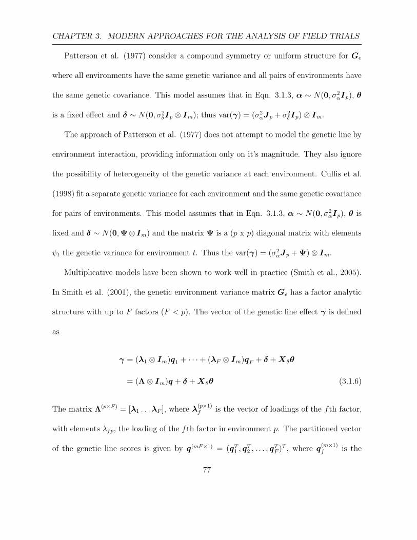
CHAPTER 3. MODERN APPROACHES FOR THE ANALYSIS OF FIELD TRIALS
Patterson et al. (1977) consider a compound symmetry or uniform structure for Ge
where all environments have the same genetic variance and all pairs of environments have
the same genetic covariance. This model assumes that in Eqn. 3.1.3, α ∼ N(0, σ2αIp), θ
is a fixed effect and δ ∼ N(0, σ2δIp ⊗ Im); thus var(γ) = (σ2
αJp + σ2δIp) ⊗ Im.
The approach of Patterson et al. (1977) does not attempt to model the genetic line by
environment interaction, providing information only on it’s magnitude. They also ignore
the possibility of heterogeneity of the genetic variance at each environment. Cullis et al.
(1998) fit a separate genetic variance for each environment and the same genetic covariance
for pairs of environments. This model assumes that in Eqn. 3.1.3, α ∼ N(0, σ2αIp), θ is
fixed and δ ∼ N(0,Ψ⊗Im) and the matrix Ψ is a (p x p) diagonal matrix with elements
ψt the genetic variance for environment t. Thus the var(γ) = (σ2αJp + Ψ) ⊗ Im.
Multiplicative models have been shown to work well in practice (Smith et al., 2005).
In Smith et al. (2001), the genetic environment variance matrix Ge has a factor analytic
structure with up to F factors (F < p). The vector of the genetic line effect γ is defined
as
γ = (λ1 ⊗ Im)q1 + · · · + (λF ⊗ Im)qF + δ + Xθθ
= (Λ⊗ Im)q + δ + Xθθ (3.1.6)
The matrix Λ(p×F ) = [λ1 . . .λF ], where λ(p×1)f is the vector of loadings of the fth factor,
with elements λfp, the loading of the fth factor in environment p. The partitioned vector
of the genetic line scores is given by q(mF×1) = (qT1 , q
T2 , . . . , q
TF )T , where q
(m×1)f is the
77

CHAPTER 3. MODERN APPROACHES FOR THE ANALYSIS OF FIELD TRIALS
vector of genetic line scores of factor f for each of the m lines and q ∼ N(0, IF ⊗ Im).
The vector of residual genetic effects δ(mp×1) has distribution δ ∼ N(0,Ψ⊗ Im), and the
matrix Ψ is a (p x p) diagonal matrix with elements ψt the genetic variance (sometimes
referred to as the specific variance) for environment t. The vector θ is as defined in Eqn:
3.1.3 and is assumed fixed. The variance of the vector of genetic line effects γ is given by
var(γ) = ΛΛT ⊗ Im + Ψ ⊗ Im (3.1.7)
Smith et al. (2001) do not explicitly include line main effects; however their model can
be extended easily to include line main effects. Their model with a random genetic line
main effect is in fact a special case of the factor analytic model where the first set of
loadings are constrained to be equal (Smith et al., 2001). The final model considered
is where Ge is completely unstructured with p(p + 1)/2 parameters for different genetic
variances for each environment and difference genetic covariances between each pair of
environments. However, Kelly et al. (2007) found that the factor analytic model of Smith
et al. (2001) which provides an approximation to the unstructured model is generally the
preferred model over the unstructured model, because it improves the predictive accuracy
of the line empirical BLUPS. In addition, models which fit an unstructured form of Ge,
often can not be properly constrained and are therefore overparameterized making them
difficult to fit.
A summary of the variance models for Ge discussed above is shown in Table 3.1.
78

CHAPTER 3. MODERN APPROACHES FOR THE ANALYSIS OF FIELD TRIALS
Table 3.1: Summary of the variance models for Ge
Constraints for Number of
Model Name (Abbreviation) Between sites Within site parameters Reference
environment environment for
variance covariance Ge
1 Diagonal (DIAG) different zero p
2 Compound Symmetry (CS) same same 2 Patterson et al. (1977)
3 (DIAG/CS) different same p + 1 Cullis et al. (1998)
4 Factor analytic order F a different different pF + p− Smith et al. (2001)
(XFAF ) F (F − 1)/2
5 Unstructured (US) different different p(p + 1)/2
a F is the number of factors, p is the number of sites
The final model, referred to hereafter as the Standard model, can be presented as
y = Xτ + Zgg + Zuu + η (3.1.8)
where X is partitioned as [Xe Zg1mp ZgXθ] and τ is partitioned as [τ Te µ θT ]T , Zuu
and η are as defined previously and g(mp×1) is the vector of m genetic line effects in each
of p environments where
g = Zαα + δ
for model 1, 2, 3 and 5 (Table 3.1) and
g = (Λ ⊗ Im)q + δ − 1mpµ
for model 4 (Table 3.1).
79
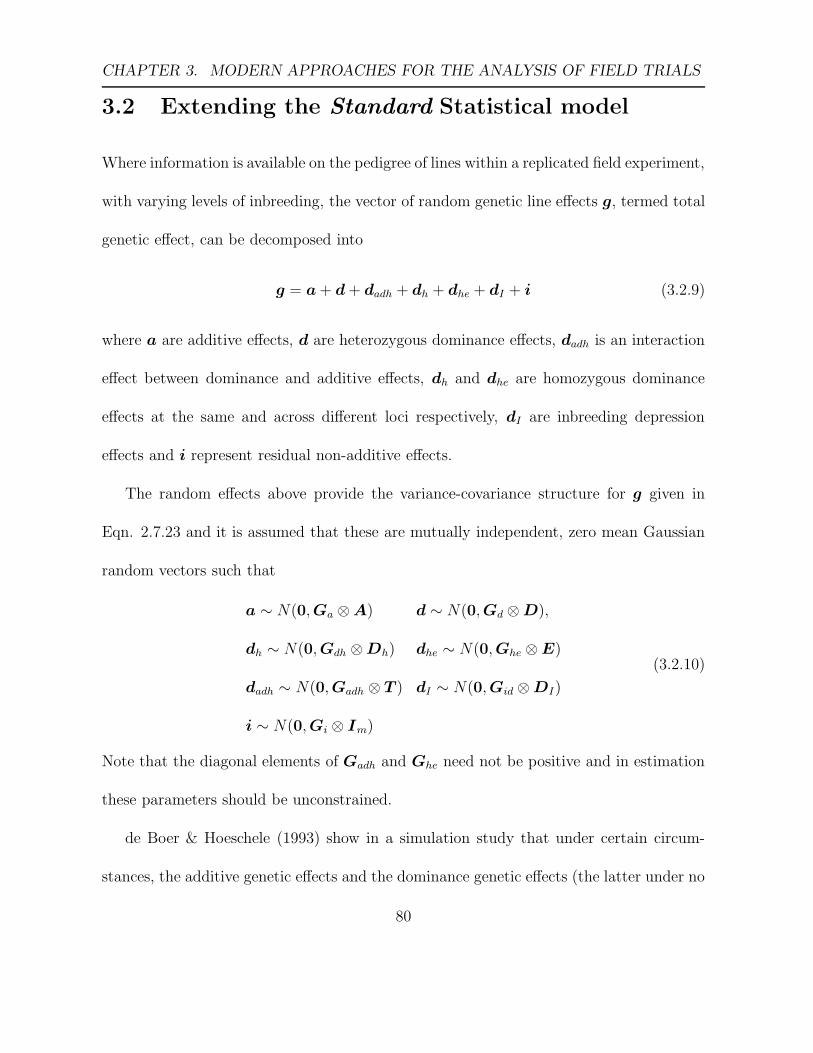
CHAPTER 3. MODERN APPROACHES FOR THE ANALYSIS OF FIELD TRIALS
3.2 Extending the Standard Statistical model
Where information is available on the pedigree of lines within a replicated field experiment,
with varying levels of inbreeding, the vector of random genetic line effects g, termed total
genetic effect, can be decomposed into
g = a + d + dadh + dh + dhe + dI + i (3.2.9)
where a are additive effects, d are heterozygous dominance effects, dadh is an interaction
effect between dominance and additive effects, dh and dhe are homozygous dominance
effects at the same and across different loci respectively, dI are inbreeding depression
effects and i represent residual non-additive effects.
The random effects above provide the variance-covariance structure for g given in
Eqn. 2.7.23 and it is assumed that these are mutually independent, zero mean Gaussian
random vectors such that
a ∼ N(0,Ga ⊗ A) d ∼ N(0,Gd ⊗ D),
dh ∼ N(0,Gdh ⊗ Dh) dhe ∼ N(0,Ghe ⊗ E)
dadh ∼ N(0,Gadh ⊗ T ) dI ∼ N(0,Gid ⊗ DI)
i ∼ N(0,Gi ⊗ Im)
(3.2.10)
Note that the diagonal elements of Gadh and Ghe need not be positive and in estimation
these parameters should be unconstrained.
de Boer & Hoeschele (1993) show in a simulation study that under certain circum-
stances, the additive genetic effects and the dominance genetic effects (the latter under no
80

CHAPTER 3. MODERN APPROACHES FOR THE ANALYSIS OF FIELD TRIALS
inbreeding) provide an accurate approximation to the full matrix. In particular, de Boer
& Hoeschele (1993) show that the prediction of the additive and dominance genetic ef-
fects has only slightly reduced accuracy in traits affected by a finite number of loci and
inbreeding. This reduction in accuracy occurred where the dominance variance was large
relative to the additive variance. This approach is used in animal and some plant breed-
ing situations where mixed models and pedigrees are standard. Here a model is fitted
in which the full dominance matrix (i.e. under varying levels of inbreeding) is included,
so that the leading two terms of Eqn. 3.2.9 are represented as well as an independent
residual component, so the simplified model referred to here as the Extended model for g
is
g = a + d + i (3.2.11)
(see Oakey et al., 2007), where a(mp×1) are additive line effects, d(mp×1) are dominance line
effects and here i(mp×1) represent residual non-additive line effects (the latter two effects
are jointly referred to as non-additive effects). The residual non-additive line effects i in
this model attempt to account for the non-additive effects in Eqn. 3.2.9 not explicitly
fitted.
It then follows that the variance of g is
var(g) = Ga ⊗ A + Gd ⊗ D + Gi ⊗ Im (3.2.12)
The additive, dominance and residual non-additive genetic variance matrices across en-
vironments are Ga, Gd and Gi respectively. These matrices have diagonal elements that
81

CHAPTER 3. MODERN APPROACHES FOR THE ANALYSIS OF FIELD TRIALS
are the genetic variances for the individual sites and off-diagonal elements that are the
genetic covariances between pairs of sites. The form of these matrices for the different
genetic terms need not be the same. The matrix A(m×m) = {Ajk} is the known additive
relationship matrix defined by Eqn. 2.8.24. The matrix D(m×m) = {Djk} is the known
dominance relationship matrix between line j who has parents Y and Z and line k, who
has parents U and V , and is defined in Section 2.9.
Notice that the Extended model has the Standard model as a sub-model. In the Stan-
dard model discussed in Section 3.1.2, g is not partitioned so that var(g) = Gi ⊗ Im,
where Im is a (m×m) identity matrix. Thus, in the Standard model, an overall random
genetic effect is fitted where lines are assumed independent. Models where g = a have
been fitted by Panter & Allen (1995), Durel et al. (1998), Dutkowski et al. (2002), Davik
& Honne (2005) and Crossa et al. (2006), estimate additive effects or breeding values
only.
The Extended model which partition the genetic line effect, still gives an overall total
genetic effect (g) and therefore an estimate of line performance which is of interest to
breeders. The additive line effects (a) should be estimated with less bias than models
which excluded non-additive effects (van der Werf & de Boer, 1989, Hoeschele & Van-
Raden, 1991 and Lu et al., 1999) and the dominance effects (d) give an indication of
how well the genes from an individual’s parents combine. Thus all effects that may be of
interest to breeders are obtained from a single model.
82
CHAPTER 3. MODERN APPROACHES FOR THE ANALYSIS OF FIELD TRIALS
These models will later be demonstrated with two practical examples. In the wheat
example of Chapter 4, as the lines have been inbred for at least five generations they are
assumed homozygous due to inbreeding, and therefore the dominance effect of a line is
assumed to be zero. Residual non-additive effects will therefore reflect epistatic effects. In
the sugarcane example of Chapter 5, the lines are hybrid crops so that the heterozygous
dominance effects and residual non-additive effects should be estimable. The residual
non-additive genetic line effects may include inbreeding depression effects, homozygous
dominance effects at the same and across different loci, the covariance between additive
and dominance effects and epistatic effects.
3.3 Fitting the dominance genetic effect d
The dominance relationship between two individuals is defined by the relationships be-
tween their parents. Individuals from the same family (i.e. same parents) therefore share
the same dominance relationships. If a pedigree contains many individuals from the same
family, the dominance relationship between these individuals can be summarized in a
reduced form by considering two components; one relating to between family effects and
the other relating to within family line effects (Hoeschele & VanRaden, 1991). Hoeschele
& VanRaden (1991) suggested that the between family effects could be included in the
model and the within family line effects be obtained by back-solving. Here we extend
their approach by including both the between family effects and within family line effects
83

CHAPTER 3. MODERN APPROACHES FOR THE ANALYSIS OF FIELD TRIALS
in the model. This means that the total dominance effect is predictable.
The de Boer & Hoeschele (1993) method of calculating the dominance matrix presented
in Section 2.9 is computationally complex. In particular, all possible gamete pairs relating
to individuals of the pedigree and ancestral gamete pairs are identified and dominance
relationships are determined for all gamete pairs. As there are often more gamete pairs
than individuals (in the example of Table 2.4 there were 14 gamete pairs from a pedigree
of 4 individuals) many calculations are required.
Hoeschele & VanRaden (1991) noted that the dominance relationship between two
individuals is defined by the relationships between their parents. Individuals from the
same family (i.e. same parents) therefore share the same dominance relationships. If
a pedigree contains many individuals from the same family, the dominance relationship
between these individuals can be summarized in a reduced form by considering two com-
ponents; one relating to the dominance relationship between families and the other to
within family dominance relationships.
Consider, the vector of dominance effects d(mp×1) = {djt}, where djt is the dominance
effect of the jth line (j = 1, . . . , m) in the tth environment (t = 1, . . . , p). This vector
can be partitioned (without loss of information) into two mutually independent vectors:
a vector of dominance effects relating to between family effects d(vp×1)b = {dbqt}, where
dbqt is the dominance between family effect for the qth family (with q = 1, 2, . . . v, v < m)
in the tth environment and a vector of dominance effects relating to within family line
84

CHAPTER 3. MODERN APPROACHES FOR THE ANALYSIS OF FIELD TRIALS
effects d(mp×1)w = {dwjt}, where dwjt is the within family line effect for the jth line in the
tth environment.
A particular line j from family q and environment t will have its dominance effect
defined as
djt = dbjt + dwjt = dbqt + dwjt (3.3.13)
where dbjt is equivalent to the between family effect dbqt, and dwjt is as defined above.
Thus d can be written as
d = Zbdb + dw
where Zb is a (mp× vp) matrix relating lines to families within environments.
The between family dominance effect db has distribution db ∼ N(0,Gd ⊗ Db), where
D(v×v)b = {Dbqαqβ
} is the known between family dominance relationship matrix for families
qα and qβ with parents Y , Z and U , V respectively. The dominance within family line
effect dw has distribution dw ∼ N(0,Gd⊗Dw), where D(m×m)w = diag{Dwj} is the known
within family line dominance relationship matrix for individual j. The elements of Db
and Dw are now developed, by modification of the algorithm of de Boer & Hoeschele
(1993).
Db is a symmetric covariance-variance matrix with diagonal terms which correspond
to the between family variance and the off-diagonal terms which correspond to covariances
between families. Hoeschele & VanRaden (1991) noted that if j and k are lines in the
85

CHAPTER 3. MODERN APPROACHES FOR THE ANALYSIS OF FIELD TRIALS
same family q with the same parents Y and Z (i.e. they are full sibs), then
cov(dbjt, dbkt) = cov(dbqt, dbqt)
=⇒ cov(dbjt, dbkt) = var(dbqt) (3.3.14)
(Note: here in addition to Hoeschele & VanRaden (1991), it is assumed that j and k
are both from environment t for completeness. Therefore, Eqn. 3.3.14 indicates that the
diagonal terms of Db are defined by the covariances between full-siblings.
Initially, consider the small example pedigree of Table 2.4. Individuals C and D are
full-siblings from the same family that is they have the same mother and father. The
dominance covariance between these individuals is the dominance value between their
gamete pairs 65 and 87 and is given by M3(87, 65) = 0.1875. By examining how this is
determined using the algorithm of de Boer & Hoeschele (1993) (initially) using the full
pedigree of Table 2.4, the diagonal elements of the between dominance matrix Db, based
on a family pedigree can be deduced. Consider the dominance value between gamete pairs
87 and 65. Note from Table 2.6, gamete 8 has parental gametes 2 and 3, (the same as
gamete 6) then according to the rules of de Boer & Hoeschele (1993).
M3(87, 65) =1
2[M3(73, 65) + M3(72, 65)]
=1
2[0.25 + 0.125] = 0.1875
The family pedigree of the example pedigree (Table 2.4) is shown in Table 3.2.
86
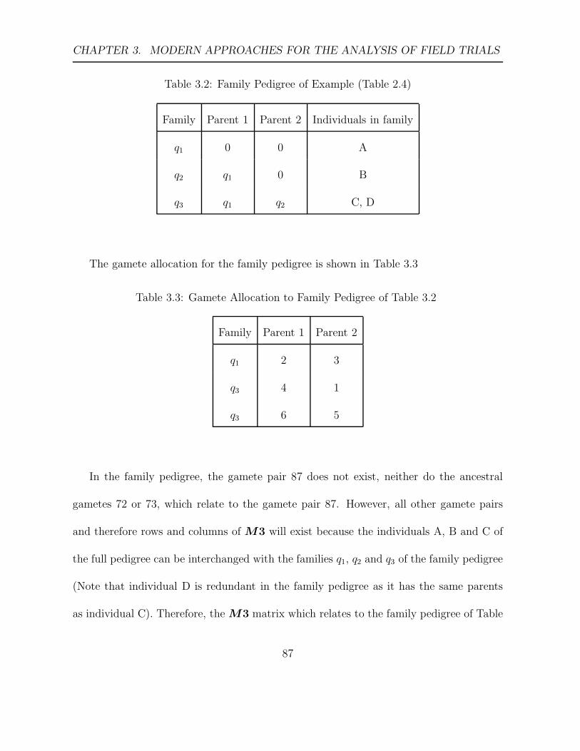
CHAPTER 3. MODERN APPROACHES FOR THE ANALYSIS OF FIELD TRIALS
Table 3.2: Family Pedigree of Example (Table 2.4)
Family Parent 1 Parent 2 Individuals in family
q1 0 0 A
q2 q1 0 B
q3 q1 q2 C, D
The gamete allocation for the family pedigree is shown in Table 3.3
Table 3.3: Gamete Allocation to Family Pedigree of Table 3.2
Family Parent 1 Parent 2
q1 2 3
q3 4 1
q3 6 5
In the family pedigree, the gamete pair 87 does not exist, neither do the ancestral
gametes 72 or 73, which relate to the gamete pair 87. However, all other gamete pairs
and therefore rows and columns of M3 will exist because the individuals A, B and C of
the full pedigree can be interchanged with the families q1, q2 and q3 of the family pedigree
(Note that individual D is redundant in the family pedigree as it has the same parents
as individual C). Therefore, the M3 matrix which relates to the family pedigree of Table
87
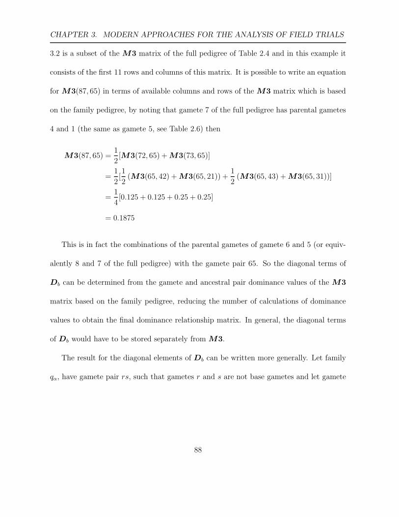
CHAPTER 3. MODERN APPROACHES FOR THE ANALYSIS OF FIELD TRIALS
3.2 is a subset of the M3 matrix of the full pedigree of Table 2.4 and in this example it
consists of the first 11 rows and columns of this matrix. It is possible to write an equation
for M3(87, 65) in terms of available columns and rows of the M3 matrix which is based
on the family pedigree, by noting that gamete 7 of the full pedigree has parental gametes
4 and 1 (the same as gamete 5, see Table 2.6) then
M3(87, 65) =1
2[M3(72, 65) + M3(73, 65)]
=1
2[1
2(M3(65, 42) + M3(65, 21)) +
1
2(M3(65, 43) + M3(65, 31))]
=1
4[0.125 + 0.125 + 0.25 + 0.25]
= 0.1875
This is in fact the combinations of the parental gametes of gamete 6 and 5 (or equiv-
alently 8 and 7 of the full pedigree) with the gamete pair 65. So the diagonal terms of
Db can be determined from the gamete and ancestral pair dominance values of the M3
matrix based on the family pedigree, reducing the number of calculations of dominance
values to obtain the final dominance relationship matrix. In general, the diagonal terms
of Db would have to be stored separately from M3.
The result for the diagonal elements of Db can be written more generally. Let family
qα, have gamete pair rs, such that gametes r and s are not base gametes and let gamete
88

CHAPTER 3. MODERN APPROACHES FOR THE ANALYSIS OF FIELD TRIALS
r have parental gametes y and z and gamete s have parental gametes u and v, then
Dbqαqα= 0.5[0.5 (M3(rs, yu) + M3(rs, yv)) + 0.5 (M3(rs, zu) + M3(rs, zv))]
= 0.25[M3(rs, yu) + M3(rs, yv) + M3(rs, zu) + M3(rs, zv)]
The off-diagonal terms of Db are based on the reduced form of the family M3 matrix,
relating to the dominance values between gamete pairs that are represented in the pedi-
gree.
Now consider the determination of the elements of Dw. Hoeschele & VanRaden (1991)
showed
var(djt) = var(dbjt) + var(dwjt)
so that the diagonal terms of Dw are defined as
var(dwjt) = var(djt) − var(dbqt) (3.3.15)
(Note: again in addition to Hoeschele & VanRaden (1991), it is assumed that j and k are
both from environment t for completeness.)
Thus the diagonal terms of Dw for individual j from family qα with gamete pair rs,
such that gametes r and s are not base gametes and where gamete r has parental gametes
y and z and gamete s has parental gametes u and v, can be determined by
M3(rs, rs) − 0.25[M3(rs, yu) + M3(rs, yv) + M3(rs, zu) + M3(rs, zv)]
89

CHAPTER 3. MODERN APPROACHES FOR THE ANALYSIS OF FIELD TRIALS
Recall that as Dw is a diagonal matrix, the off-diagonal terms are zero. Thus the reduced
family pedigree based on familial relationships needs to be used to create the reduced
form of M3 from which Db and Dw can be formed. The variance matrix of d can be
written in terms of Db and Dw namely
var(d) = var(Zbdb + dw) = ZbDbZTb + Dw = D (3.3.16)
If a completely balanced data set is considered, such that the number of replicates rq of
the qth family is the same across all v families, then Zb = Iv ⊗ 1rvwhere Iv is a (v x v)
identity matrix and 1(rv x 1)rv
is a vector of ones and m = vrv, then
D = ZbDbZTb + Dw
= (Iv ⊗ 1rv)(Db ⊗ 1)(Iv ⊗ 1T
rv) + Dw
D = (Db ⊗ J rv) + Dw (3.3.17)
where J rv= 1rv
1Trv
is a (rv x rv) matrix of ones. Thus D is partitioned into two matrices
(Db ⊗ J rv) and Dw. The equivalent equation under no inbreeding is given by Hoeschele
& VanRaden (1991) as D = 0.25WFW T + 0.75I where W = Zb, Db = 0.25F and
Dw = 0.75I. The equation under no inbreeding gives a result for the case where either r
or s or both are base gametes. Hence
Dbqαqα= 0.25
and therefore the corresponding value for individuals from the family qα is
Dwqα= 0.75
90

CHAPTER 3. MODERN APPROACHES FOR THE ANALYSIS OF FIELD TRIALS
For the example, consider the family pedigree of the example of Table 2.4, using the rules
defined above the between family dominance matrix Db is
Db =q1
q2
q3
q1 q2 q3
0.25 0 0.25
0 0.25 0.25
0.25 0.25 0.1875
and the within family dominance matrix is
Dw =
A
B
C
D
A B C D
0.75 0 0 0
0 0.75 0 0
0 0 0.5625 0
0 0 0 0.5625
For the example pedigree of Table 2.4 Zb is
Zb =
A
B
C
D
q1 q2 q3
1 0 0
0 1 0
0 0 1
0 0 1
91
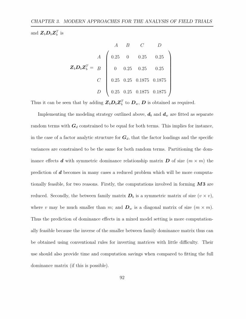
CHAPTER 3. MODERN APPROACHES FOR THE ANALYSIS OF FIELD TRIALS
and ZbDbZTb is
ZbDbZTb =
A
B
C
D
A B C D
0.25 0 0.25 0.25
0 0.25 0.25 0.25
0.25 0.25 0.1875 0.1875
0.25 0.25 0.1875 0.1875
Thus it can be seen that by adding ZbDbZTb to Dw, D is obtained as required.
Implementing the modeling strategy outlined above, db and dw are fitted as separate
random terms with Gd constrained to be equal for both terms. This implies for instance,
in the case of a factor analytic structure for Gd, that the factor loadings and the specific
variances are constrained to be the same for both random terms. Partitioning the dom-
inance effects d with symmetric dominance relationship matrix D of size (m × m) the
prediction of d becomes in many cases a reduced problem which will be more computa-
tionally feasible, for two reasons. Firstly, the computations involved in forming M3 are
reduced. Secondly, the between family matrix Db is a symmetric matrix of size (v × v),
where v may be much smaller than m; and Dw is a diagonal matrix of size (m × m).
Thus the prediction of dominance effects in a mixed model setting is more computation-
ally feasible because the inverse of the smaller between family dominance matrix thus can
be obtained using conventional rules for inverting matrices with little difficulty. Their
use should also provide time and computation savings when compared to fitting the full
dominance matrix (if this is possible).
92

CHAPTER 3. MODERN APPROACHES FOR THE ANALYSIS OF FIELD TRIALS
The elements of Db and Dw can thus be obtained by modification of the de Boer &
Hoeschele (1993) algorithm, where the full or usual pedigree is used to form a reduced
pedigree based on familial relationships.
By partitioning the dominance effect and in turn the dominance relationship matrix,
the potential information required to be input in the form of dominance relationships
between individuals can be reduced if the number of families is less than the number of
individuals. Thus the prediction of dominance effects in a mixed model setting is more
computationally feasible because the inverse of the smaller between family dominance
matrix thus can be obtained using conventional rules for inverting matrices with little
difficulty.
Notice that the inverse of the full dominance matrix D can be found using smaller
and simpler matrices as
D−1 = D−1w − D−1
w Zb(ZTb D−1
w Zb + D−1b )−1ZT
b D−1w
although using the between and within family structures may be of interest to breeders.
Incorporating this partitioned vector of genetic line effects into the Standard model
(Eqn. 3.1.8), the Extended model is
y = Xτ + Zga + ZgZbdb + Zgdw + Zgi + Zuu + η (3.3.18)
where terms are as defined previously.
Thus the algorithm for the between and within dominance matrices is described in
Sections 3.3.1 to 3.3.7.
93

CHAPTER 3. MODERN APPROACHES FOR THE ANALYSIS OF FIELD TRIALS
3.3.1 Determination of the family pedigree
The family pedigree is essentially a subset of the full pedigree, where individuals from the
same family are omitted from the pedigree unless they are themselves parents. If members
of a family are themselves parents then they need to be included in the family pedigree.
This is because they will have a different dominance relationship with their offspring than
other family members will have. Notice that the pedigree in Table 2.8 for instance could
not be reduced as individual C would have a different relationship to individual E than
individual D, even though individual D comes from the same family as individual C, this
is because individual C is a parent of individual E, whereas individual D is not.
3.3.2 Forming gamete pairs
The algorithm for determining the between and within dominance matrices then proceeds
with forming the gamete pairs, given in Section 2.9.7, but instead of the full pedigree of
individuals use the family pedigree.
3.3.3 Determining the dominance relationship between gamete
pairs
The matrix M3 of the dominance relationships between all possible gamete pairs is now
created using the rules presented in Section 2.9.6. The off-diagonal elements of this matrix
of the gamete pairs which correspond to families in the pedigree form the off-diagonals
94

CHAPTER 3. MODERN APPROACHES FOR THE ANALYSIS OF FIELD TRIALS
of the between dominance matrix Db. The diagonal elements of Db, where family qα,
has gamete pair rs, such that gametes r and s are not base gametes and gamete r has
parental gametes y and z and gamete s has parental gametes u and v, are
Dbqαqα= 0.25[M3(rs, yu) + M3(rs, yv) + M3(rs, zu) + M3(rs, zv)]
The special case where, one or both of the gametes in the pair rs of the family qα are
base gametes results in diagonal terms for Db as follows
Dbqαqα= 0.25
This latter result is the same as that obtained under no inbreeding (Hoeschele & Van-
Raden, 1991).
The diagonal Dw matrix has diagonal terms for individual j from family qα with
gamete pair rs, such that gametes r and s are not base gametes and where gamete r
has parental gametes y and z and gamete s has parental gametes u and v, that can be
determined by
M3(rs, rs) − 0.25[M3(rs, yu) + M3(rs, yv) + M3(rs, zu) + M3(rs, zv)]
Again the special case of the diagonal term of Dw, for individual j, from family qα with
gamete pair rs, such that either gamete r or s are base gametes is
Dwj = 0.75 (3.3.19)
The diagonal elements of Db and Dw are thus formed from M3 and would need to
be stored separately from M3.
95

CHAPTER 3. MODERN APPROACHES FOR THE ANALYSIS OF FIELD TRIALS
3.3.4 The dominance genetic effect assuming no inbreeding
The method for calculating the dominance relationship matrix under no inbreeding pre-
sented in Section 2.11 can also be adapted so that the between and within dominance
matrices are calculated. The assumption of no inbreeding may be necessary in order
to make the calculation of the dominance between and within matrices computationally
feasible.
3.3.5 Determination of the family pedigree
First, the family pedigree needs to be determined. Proceed as in Section 3.3.1.
3.3.6 Gamete allocation and the probability of gamete inheri-
tance
The algorithm for determining the between and within dominance matrices then proceeds
with gamete allocation (Section 2.11.1) and determining the probability of gamete inher-
itance (Section 2.11.2), but instead of the full pedigree of individuals (see Table 2.4) use
the family pedigree (see Table 3.2). Note the table of probabilities for the family pedigree
will be a subset of the table of probabilities for the full pedigree.
96

CHAPTER 3. MODERN APPROACHES FOR THE ANALYSIS OF FIELD TRIALS
3.3.7 Calculating between and within dominance relationships
For the calculation of dominance values of Db and Dw, use the following rules in place
of those in Section 2.11.3, so that the results of Hoeschele & VanRaden (1991) given in
Equations 3.3.14 and 3.3.15 will again be applied.
Let each row of the table of probabilities be considered a vector, for example let the
probabilities of the base gametes for the male parent of family qα be qTαm. From Eqn.
3.3.14, the diagonal terms of Db are defined by the covariances between full-siblings and
are therefore given by
Dbqαqα= sum
(
(qTαmqαf ).(qT
αmqαf ))
+ sum(
(qTαfqαm).(qT
αmqαf ))
− 2(
diag(qTαmqαf )
(
diag(qTαmqαf)
)T)
(3.3.20)
where . indicates the Hadamard product of the two matrices. The off-diagonal terms of
Db are given by
Dbqαqβ= sum
(
(qTαmqαf ).(qT
βmqβf ))
+ sum(
(qTαfqαm).(qT
βmqβf ))
− 2(
diag(qTαmqαf )
(
diag(qTβmqβf)
)T)
(3.3.21)
Note that Eqn. 3.3.21 is essentially the same formulation given for the dominance Djk
between individuals j and k in Eqn. 2.11.50. Here individual j and individual k are
substituted for families qα and qβ respectively.
The diagonal terms of Dw for individual j from family qα, using the result of 3.3.15
97

CHAPTER 3. MODERN APPROACHES FOR THE ANALYSIS OF FIELD TRIALS
are:
Dwj = 1 − qαmqTαf
− sum(
(qTαmqαf ).(qT
αmqαf ))
− sum(
(qTαfqαm).(qT
αmqαf))
+ 2(
diag(qTαmqαf )
(
diag(qTαmqαf)
)T)
= 1 − qαmqTαf −Dbqαqα
(3.3.22)
3.4 Estimation and Fitting
When fitting the models described above, a hierarchical or incremental approach must
be taken. In the first instance the Standard model with a diagonal variance structure
(Model 1, Table 3.1) is fitted to determine the non-genetic or environmental parameters
appropriate for each environment. Examination of diagnostics include plotting a sam-
ple variogram for examining spatial covariance structure and plots of residuals against
row(column) number for each column(row) (see Gilmour et al., 1997 for details) deter-
mines which (if any) spatial terms may be needed. Once an appropriate non-genetic
model is determined, the genetic effects of the Extended model can be incorporated and
fitted. There will be situations where one or more of the REML estimates of the additive,
dominance and epistatic genetic variances are zero at a particular environment; thus the
particular component is not present. This also means that correlations between the sites
with zero estimated genetic variance and other sites cannot be estimated. To determine
98

CHAPTER 3. MODERN APPROACHES FOR THE ANALYSIS OF FIELD TRIALS
if genetic variance is present for each component at each environment, a model which as-
sumes zero correlations between sites is initially fitted for all three components. Variance
models for Ga, Gd and Gi can then be chosen which exclude sites with no estimable ad-
ditive, dominance or residual non-additive variance respectively. For environments with
positive genetic variances the aim is to fit a factor analytic structure as these have been
shown to work well in practice (Smith et al., 2005). However, factor analytic structures
can be difficult to fit. For a single factor model, simpler models should be used as a basis
for initial parameter estimates. It is recommended that the model of Cullis et al. (1998)
be fitted and initial estimates of the genetic variance for each environment from this model
be used in the factor analytic structure with one factor. If the number of environments
is reasonably large and the percentage variance accounted for by a single factor model is
small, then a factor analytic structure with two factors can also be attempted. The initial
estimates for the genetic variances of each environment for a two factor model should be
based on the results of the one factor model. When fitting models with more than one
factor, linear constraints are imposed on the loadings to ensure the solution is unique
(Smith et al., 2001). For a two factor model, one of the loadings of the second factor is
set to zero.
For models that are nested a residual or restricted maximum likelihood ratio test
(REMLRT) can be used to compare models. The REMLRT statistic is minus twice the
difference of the two model REML log-likelihoods and is asymptotically distributed as
99
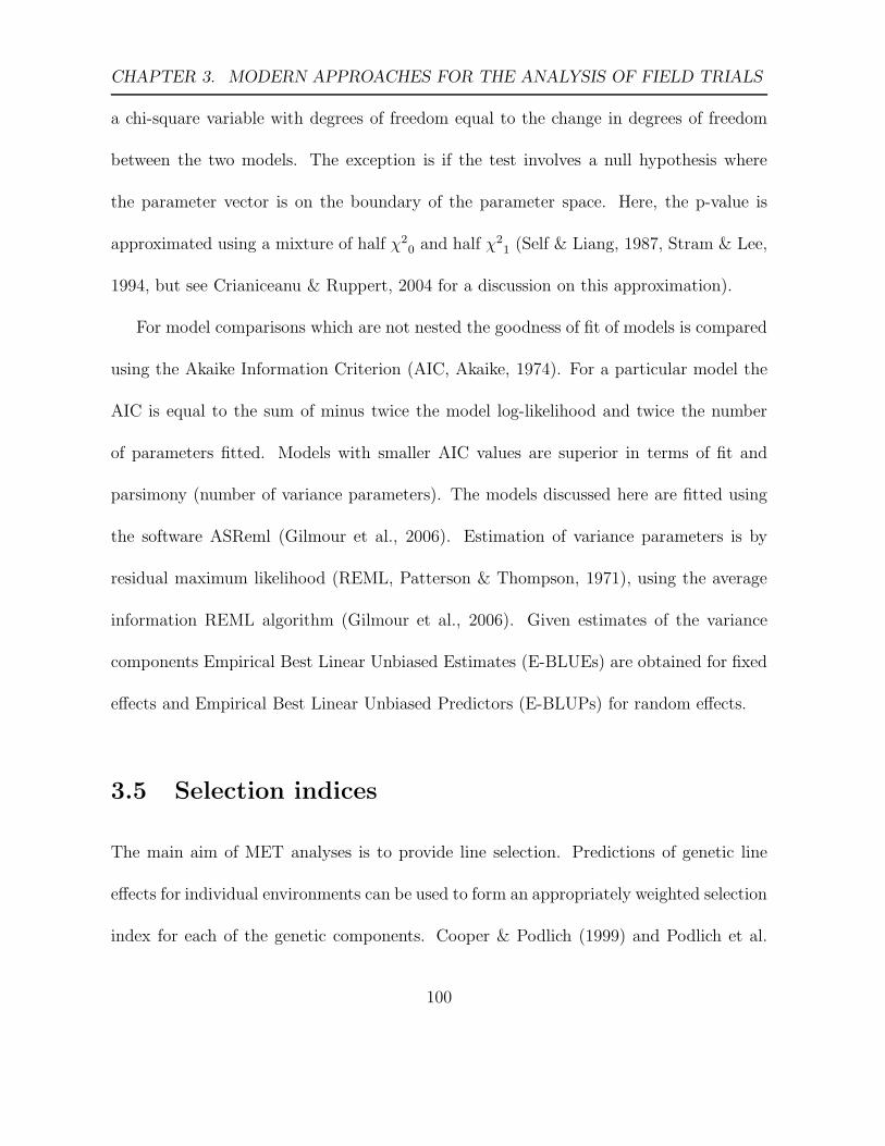
CHAPTER 3. MODERN APPROACHES FOR THE ANALYSIS OF FIELD TRIALS
a chi-square variable with degrees of freedom equal to the change in degrees of freedom
between the two models. The exception is if the test involves a null hypothesis where
the parameter vector is on the boundary of the parameter space. Here, the p-value is
approximated using a mixture of half χ20 and half χ2
1 (Self & Liang, 1987, Stram & Lee,
1994, but see Crianiceanu & Ruppert, 2004 for a discussion on this approximation).
For model comparisons which are not nested the goodness of fit of models is compared
using the Akaike Information Criterion (AIC, Akaike, 1974). For a particular model the
AIC is equal to the sum of minus twice the model log-likelihood and twice the number
of parameters fitted. Models with smaller AIC values are superior in terms of fit and
parsimony (number of variance parameters). The models discussed here are fitted using
the software ASReml (Gilmour et al., 2006). Estimation of variance parameters is by
residual maximum likelihood (REML, Patterson & Thompson, 1971), using the average
information REML algorithm (Gilmour et al., 2006). Given estimates of the variance
components Empirical Best Linear Unbiased Estimates (E-BLUEs) are obtained for fixed
effects and Empirical Best Linear Unbiased Predictors (E-BLUPs) for random effects.
3.5 Selection indices
The main aim of MET analyses is to provide line selection. Predictions of genetic line
effects for individual environments can be used to form an appropriately weighted selection
index for each of the genetic components. Cooper & Podlich (1999) and Podlich et al.
100

CHAPTER 3. MODERN APPROACHES FOR THE ANALYSIS OF FIELD TRIALS
(1999) show through computer simulation that weighted selection strategies perform as
well or better than the traditional unweighted strategies. In particular, the performance
of weighted strategies is better when only a few environments are sampled in a MET
or when there is a lack of genetic correlation between environments. The weights may
be chosen in a number of ways. Cooper et al. (1996) suggest giving bigger weights to
environments that are more representative of target environments and Kelly et al. (2007)
consider merit in equal weights across all environments. Ultimately, the weights given to
the environments will to some extent depend on the breeders knowledge of each of the
environments. Let wta, wtd and wti, be the weights for environment t for the additive,
dominance and residual non-additive selection indices and at, dt(= dbt + dwt) and it be
the vectors of genetic line E-BLUPs for the additive, dominance and non-residual effects
at environment t respectively. The selection index ma for additive genetic line effects
across p trials is
ma = w1aa1 + . . .+ wpaap,
the selection index md for dominance genetic line effects is
md = w1dd1 + . . .+ wpddp,
and the selection index mi for residual non-additive genetic line effects is
mi = w1ii1 + . . .+ wpiip,
101
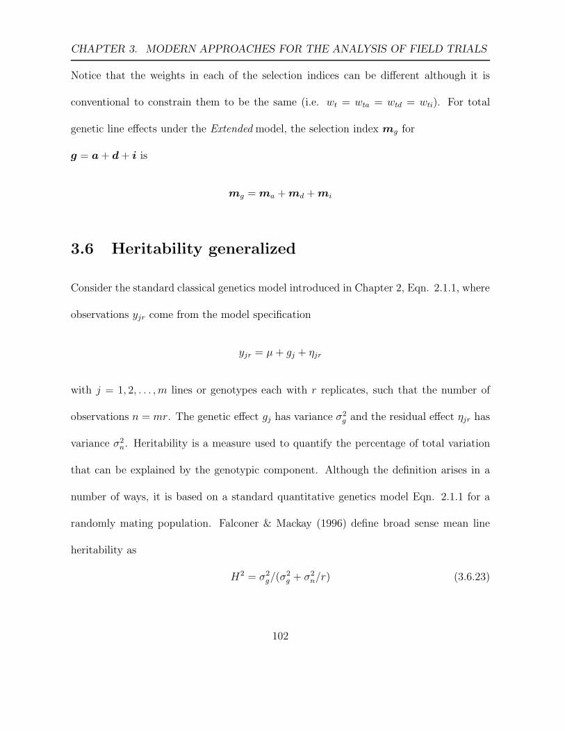
CHAPTER 3. MODERN APPROACHES FOR THE ANALYSIS OF FIELD TRIALS
Notice that the weights in each of the selection indices can be different although it is
conventional to constrain them to be the same (i.e. wt = wta = wtd = wti). For total
genetic line effects under the Extended model, the selection index mg for
g = a + d + i is
mg = ma + md + mi
3.6 Heritability generalized
Consider the standard classical genetics model introduced in Chapter 2, Eqn. 2.1.1, where
observations yjr come from the model specification
yjr = µ+ gj + ηjr
with j = 1, 2, . . . , m lines or genotypes each with r replicates, such that the number of
observations n = mr. The genetic effect gj has variance σ2g and the residual effect ηjr has
variance σ2n. Heritability is a measure used to quantify the percentage of total variation
that can be explained by the genotypic component. Although the definition arises in a
number of ways, it is based on a standard quantitative genetics model Eqn. 2.1.1 for a
randomly mating population. Falconer & Mackay (1996) define broad sense mean line
heritability as
H2 = σ2g/(σ
2g + σ2
n/r) (3.6.23)
102
CHAPTER 3. MODERN APPROACHES FOR THE ANALYSIS OF FIELD TRIALS
while narrow sense mean line heritability requires a pedigree and an associated additive
relationship matrix and is given by
h2 = σ2a/(σ
2a + σ2
n/r) (3.6.24)
The model presented for analysis of trial data, (Eqn. 3.3.18), does not adhere to the
standard assumptions. Thus Eqn. 3.6.23 and Eqn 3.6.24 may not be appropriate, and
a generalised form of heritability needs to be defined. Cullis et al. (2007) consider the
problem of defining heritability in more complex settings. Their definition is based on
average pairwise prediction error variance that is appropriate for general error covariance
matrices and diagonal genetic covariance matrices.
Here, a generalised definition of heritability is defined using a generic mixed model.
Thus suppose
y = Xτ + Zgg + Zuu + η (3.6.25)
where g ∼ N(0,G), u ∼ N(0,U) and η ∼ N(0,R). The Standard model (Eqn. 3.1.8)
and Extended model (Eqn. 3.3.18) are specific cases. Note that
y ∼ N(Xτ ,V )
where V = ZgGZTg + ZuUZT
u + R.
To develop a general approach, heritability is defined as the squared correlation be-
tween the realized (or predicted) and the true genetic effect (Falconer & Mackay, 1996,
p160). This definition implicitly assumes a single genetic effect, whereas in general there
103

CHAPTER 3. MODERN APPROACHES FOR THE ANALYSIS OF FIELD TRIALS
is a vector of genetic effects. In the standard quantitative model this is not an issue,
because genetic effects have a ‘common heritability’. In more complex models this no
longer holds.
To reduce the genetic effect to a scalar quantity, consider a linear combination of the
true genetic effects, namely cT g, and the corresponding predicted genetic effects, namely
cT g. There are many choices for c and the derivation of generalized heritability results
in a canonical set of vectors c.
For the genetic effect cT g, the heritability is defined as
H2c =
cov(cT g, cT g)2
var(cT g)var(cT g)
where
cov(cT g, cT g) = cT cov(g, g)c
= cT cov(g,GZTg P V y)c using Standard results on mixed models
= cT cov(g,y)P V ZgGc see (Cullis et al., Ch 6)
= cT cov(g,Xτ + Zgg + Zuu + η)P V ZgGc
= cT cov(g,Zgg)P V ZgGc
= cT cov(g, g)ZTg P V ZgGc
= cT var(g)ZTg P V ZgGc
= cT GZTg P V ZgGc
104

CHAPTER 3. MODERN APPROACHES FOR THE ANALYSIS OF FIELD TRIALS
for
P V = V −1 − V −1X(XT V −1X)−1XT V −1 (3.6.26)
var(cT g) = cT var(g)c
= cT Gc
var(cT g) = cT var(g)c
= cT var(GZTg P V y)c
= cT GZTg P V var(y)P V ZgGc
= cT GZTg P V V P V ZgGc
= cT GZTg P V ZgGc
and therefore the generalized heritability is given by
H2c =
cT GZTg P V ZgGc
cT Gc(3.6.27)
As an overall measure of heritability is required, the vector c is chosen to maximize the
heritability subject to cT Gc = 1 (normalization with respect to G).
Consider the Lagrangian Lc,
Lc = cT GZTg P V ZgGc − ρ(cT Gc − 1) (3.6.28)
105
CHAPTER 3. MODERN APPROACHES FOR THE ANALYSIS OF FIELD TRIALS
where c is chosen to maximise the Lagrangian Lc given by Eqn 3.6.28. Thus differentiating
Lc with respect to c and setting to zero,
∂ Lc
∂c= 2GZT
g P V ZgGc − 2ρGc = 0
and therefore
GZTg P V ZgGc = ρGc
=⇒ ZTg P V ZgGc = ρc (3.6.29)
Thus c is an eigenvector of the matrix ZTg P V ZgG with eigenvalue ρ. Notice that from
Eqn. 3.6.29
=⇒ cT GZTg P V ZgGc = ρcT Gc
= ρ
using the constraint. Not only can the c that maximizes the squared correlation be found,
but a complete set of eigenvectors c for ZTg P V ZgG with associated eigenvalues. Thus
the eigenvalues provide a set of heritability components that can be used to provide an
overall measure of heritability. The vector c that maximizes H2c is an eigenvector of the
matrix ZTg P V ZgG with associated eigenvalue ρ. In fact
maxcH2c = ρ
so that this eigenvalue is a component of the full heritability and the largest eigenvalue.
106

CHAPTER 3. MODERN APPROACHES FOR THE ANALYSIS OF FIELD TRIALS
The full set of eigenvalues of ZTg P V ZgG will characterize the full heritability. Let
ρ1, ρ2, . . . , ρm be the full set of eigenvalues. Some of these eigenvalues will be zero because
of constraints on g. Suppose the last s are zero. The generalized heritability is defined as
H2 =
∑mi=1 ρi
m− s=
∑m−si=1 ρi
m− s(3.6.30)
In general, it is not possible to present analytical solutions and numerical methods must
be used to calculate the heritability. From results on mixed models (Cullis et al., Ch 6),
107

CHAPTER 3. MODERN APPROACHES FOR THE ANALYSIS OF FIELD TRIALS
GZTg P V ZgG = G − (ZT
g SZg + G−1)−1
ZTg P V ZgG = Im − G−1(ZT
g SZg + G−1)−1 (3.6.31)
where
S = R−1 − R−1X(XT R−1X)−1XT R−1 (3.6.32)
Now (ZTg SZg+G−1)−1 = CZZ is the partition of the inverse of the mixed model coefficient
matrix corresponding to g. This latter term CZZ is also equivalent to the prediction error
variance matrix for g (i.e. var(g − g)), an estimate of which is available in the software
ASReml (Gilmour et al., 2006) via the predict statement. So
ZTg P V ZgG = Im − G−1CZZ (3.6.33)
and eigenvalues of this matrix are required to determine the generalized heritability. Thus
the eigenvalue calculations can be based on Im−G−1CZZ . For large problems an approx-
imation to the generalized heritability may be very useful. Using the property that the
trace of a matrix is the sum of the eigenvalues of that matrix, an approximate heritability
is
H2 =
(
1 −tr(G−1CZZ)
m
)
and the trace term can be found by summing element by element product of the two
matrices. This ignores the possibility of zero eigenvalues. For single site analysis the
estimated CZZ can be obtained easily using the predict statement of the software ASReml
108
CHAPTER 3. MODERN APPROACHES FOR THE ANALYSIS OF FIELD TRIALS
(Gilmour et al., 2006). However, for multi-environment analysis the size of the estimated
CZZ is a limiting factor.
Now consider the generalised heritability in the standard quantitative genetics model.
The standard quantitative genetics model Eqn. 2.1.1, with m test lines each with r
replicates and n observations (such that n = mr) in vector-matrix form is
y = 1nµ+ Zgg + η (3.6.34)
where Zg = Im ⊗ 1r, X = 1n = 1m ⊗ 1r, g ∼ N(0,G = σ2gIm) is the vector of genetic
effects and η ∼ N(0,R = σ2nIn).
To evaluate the heritability, first ZTg P V ZgG is determined using the Eqn. 3.6.26 for
P V . Now
ZTg P V Zg = ZT
g V −1Zg − ZTg V −1X(XT V −1X)−1XT V −1Zg (3.6.35)
where
V = ZgGZg + R
= (Im ⊗ 1r)(σ2gIm ⊗ 1)(Im ⊗ 1T
r ) + σ2nIn
= Im ⊗ (σ2g1r1
Tr + σ2
nIn)
= Im ⊗ (σ2gJ r + σ2
nIn)
where J r is a r × r matrix of ones. The inverse of V is
V −1 = Im ⊗1
σ2n
(Ir −σ2
g
σ2n + rσ2
g
J r)
109

CHAPTER 3. MODERN APPROACHES FOR THE ANALYSIS OF FIELD TRIALS
The terms of Eqn. 3.6.35 will now be evaluated
ZTg V −1Zg = (Im ⊗ 1T
r )(Im ⊗1
σ2n
(Ir −σ2
g
σ2n + rσ2
g
J r))(Im ⊗ 1r)
=1
σ2n
Im ⊗ (1Tr 1r −
σ2g
σ2n + rσ2
g
)(1Tr J r1r)
=1
σ2n
(r −r2σ2
g
σ2n + rσ2
g
)Im
=r
σ2n
(σ2
n
σ2n + rσ2
g
)Im
=r
σ2n + rσ2
g
Im
while,
XT V −1X = (1Tm ⊗ 1T
r )(Im ⊗1
σ2n
(Ir −σ2
g
σ2n + rσ2
g
J r))(1m ⊗ 1r)
=1
σ2n
(1Tm1m) ⊗ (1T
r 1r −σ2
g
σ2n + rσ2
g
1Tr J r1r)
=m
σ2n
(r −r2σ2
g
σ2n + rσ2
g
)
=mr
σ2n
(1 −rσ2
g
σ2n + rσ2
g
)
=mr
σ2n + rσ2
g
Hence,
(XT V −1X)−1 =σ2
n + rσ2g
mr
Lastly,
ZTg V −1X = (Im ⊗ 1T
r )(Im ⊗1
σ2n
(Ir −σ2
g
σ2n + rσ2
g
J r))(1m ⊗ 1r) =r
σ2n + rσ2
g
1m
110

CHAPTER 3. MODERN APPROACHES FOR THE ANALYSIS OF FIELD TRIALS
and
XT V −1Zg = (1Tm ⊗ 1T
r )(Im ⊗1
σ2n
(Ir −σ2
g
σ2n + rσ2
g
J r))(Im ⊗ 1r) =r
σ2n + rσ2
g
1Tm
where 1Tr 1r = r and 1T
r J r1r = r2. Substituting these terms into Eqn. 3.6.35, then
ZTg P V Zg =
r
σ2n + rσ2
g
Im −r
σ2n + rσ2
g
1m(σ2
n + rσ2g
mr)
r
σ2n + rσ2
g
1Tm
=r
σ2n + rσ2
g
(Im −1
m1m1T
m)
=1
σ2n/r + σ2
g
(Im − P 1m)
where P 1m= 1m(1T
m1m)−11Tm = 1
m1m1T
m is a projection matrix onto 1m. Thus
ZTg P V ZgG =
σ2g
σ2n/r + σ2
g
(Im − P 1m) (3.6.36)
Thus the eigenvalues of Im −P 1mare required. From standard results the eigenvalues of
Im are 1 and P 1mhas m−1 eigenvalues at zero and one eigenvalue at value 1. Thus Eqn
3.6.36 has one zero eigenvalue and m − 1 repeated eigenvalues that equal H2 =σ2
g
σ2g+σ2
n/r,
which is the mean line heritability given in Eqn. 3.6.23. Thus Eqn. 3.6.30 reduces to the
mean line heritability in this case.
The narrow sense heritability can be derived by considering the standard quantitative
genetic model (Eqn. 3.6.34), with g ∼ N(0,G = σ2aA) so that lines are related with
additive relationship matrix A. In the standard case where g ∼ N(0,G = σgIm), the
generalized heritability was derived by directly calculating the eigenvalues of ZTg P V ZgG
(Eqn. 3.6.29) whereas here it is simpler to use the identity given in Eqn. 3.6.31 and derive
111

CHAPTER 3. MODERN APPROACHES FOR THE ANALYSIS OF FIELD TRIALS
the eigenvalues of the right hand side of the equation. Thus consider
ZTg SZg = ZT
g R−1Zg − ZTg R−1X(XT R−1X)−1XT R−1Zg (3.6.37)
using Eqn. 3.6.32 for S. Now, ZTg R−1Zg, ZT
g R−1X XT R−1Zg and (XT R−1X)−1 of
Eqn. 3.6.37 are evaluated
ZTg R−1Zg = (Im ⊗ 1T
r )(1
σ2n
Im ⊗ Ir)(Im ⊗ 1r) =r
σ2n
Im,
ZTg R−1X = (Im ⊗ 1T
r )(1
σ2n
Im ⊗ Ir)(1m ⊗ 1r) =r
σ2n
1m,
XT R−1Zg = (1Tm ⊗ 1T
r )(1
σ2n
Im ⊗ Ir)(Im ⊗ 1r) =r
σ2n
1Tm,
and
(XT R−1X)−1 = (1Tn (
1
σ2n
In)1n)−1 = (n
σ2n
)−1 =σ2
n
n
Substituting these results into Eqn. 3.6.37, then
ZTg SZg =
r
σ2n
Im −r
σ2n
1m(σ2
n
n)r
σ2n
1Tm
=r
σ2n
(Im −1
g1m1T
m)
=r
σ2n
(Im − P 1m) (3.6.38)
where P 1mis the projection matrix onto 1m and so substituting into Eqn. 3.6.31
ZTg P vZgG = Im −
1
σ2a
A−1[r
σ2n
(Im − P 1m) +
1
σ2a
A−1]−1
= Im − [rσ2
a
σ2n
(Im − P 1m)A + Im]−1 (3.6.39)
112
CHAPTER 3. MODERN APPROACHES FOR THE ANALYSIS OF FIELD TRIALS
Let ςi be the eigenvalues of (Im − P 1m)A; then the narrow sense heritability is
h2 =1
m− 1
m−1∑
i=1
ςiσ2a
ςiσ2a + σ2
n/r
This differs from the usual narrow sense heritability given by Eqn. 3.6.24. The generalized
definition takes into consideration the pedigree structure rather than implicitly assuming
independence of lines.
In the Extended model a broad sense heritability (H2) can be obtained by considering
G = Ga ⊗ A + Gd ⊗ D + Gi ⊗ Im (for hybrid crops) and G = Ga ⊗ A + Gi ⊗ Im (for
completely inbred lines) and a narrow sense heritability (h2) by considering G = Ga ⊗A.
113

Chapter 4
Analysis of Wheat Breeding Trials
A multi-environment trial was kindly provided by Haydn Kuchel of the Australian Grain
Technologies’ (AGT). As part of the AGTs’ national program of advanced breeding trials,
elite wheat lines are tested annually in regions around Australia. The AGT breeding
program has two aims. The first aim is to identify and select elite lines for advancement
to the next stage of testing and ultimately for commercial release. The second aim is
to identify and select elite lines for use in future crosses. Generally, line selection is for
overall performance across environments. However, lines that are particularly adapted to
specific types of environments may also be of interest. Currently, to address both aims,
AGT analyse single trials as in the Standard model described in Section 4.2.1. For the
analysis of replicated multi-environment trials, AGT use the approach of Patterson et al.
(1977) and therefore this model has been fitted here as a comparison (Model 1, Table 4.6).
The wheat lines included in the AGT trials have been inbred for at least five generations
114

CHAPTER 4. ANALYSIS OF WHEAT BREEDING TRIALS
and are therefore assumed homozygous due to inbreeding. The methodology developed
in Chapter 3 for inbred lines is used to analyse the breeding trials. The work in Section
4.2 was presented in Oakey et al. (2006).
4.1 Trial details
The data set was taken from the 2004 Stage 3 trialling program and consisted of 14 trials.
These trials are spread across the major wheat growing regions of Australia. All trials
were laid out in a rectangular column by row array of 504 plots. Most trials had an
arrangement of 12 columns by 42 rows; the exception was Narrabri which had 18 columns
by 28 rows. Plots were sown to a size of 1.32m x 5m and reduced to 1.32m x 3.2m before
anthesis by herbicide application. Seed was sown on a volume basis, aiming for an average
of 200 seeds per square metre.
A total of 253 lines were tested across the trials; 252 of these lines were elite wheat
breeding lines of interest and one line was used as a filler line. Most of the elite lines were
sown at all trials (Table 4.1), however, Coomalbidgup and Mingenew each had two elite
lines which were not sown and Narrandera and Temora each had one elite line that was
not sown. In these trials, the filler line was used to replace the missing elite lines.
115

CHAPTER 4. ANALYSIS OF WHEAT BREEDING TRIALS
Table 4.1: Details of the wheat example trialsa.
Trial Location State Number of Lines planted Mean Yield
Total Pedigree Unknown Filler (kg/ha)
1 Coomalbidgup WA 251 129 121c 1 3009
2 Coonalpyn SA 252 129 123 0 2092
3 Kapunda SA 252 129 123 0 3140
4 Merredin WA 252 129 123 0 774
5 Mingenew WA 251 129 121c 1 2255
6 Minnipa SA 252 129 123 0 743
7 Narrabri NSW 252 129 123 0 5427
8 Narrandera NSW 252 128b 123 1 1008
9 Pinnaroo SA 252 129 123 0 1848
10 Robinvale VIC 253 129 123 1 603
11 Roseworthy SA 252 129 123 0 3464
12 Scaddon WA 252 129 123 0 2952
13 Temora NSW 252 128b 123 1 2364
14 Wongan Hills WA 252 129 123 0 881
aAll trials had 504 plots, with an array of 12 columns by 42 rows, except Narrabri which had 18columns by 28 rows.
bThese trials both had the same line missingcThese trials both had the same lines missing
116

CHAPTER 4. ANALYSIS OF WHEAT BREEDING TRIALS
Trials were designed using the nearest neighbour option within Agrobase II (Agronomix,
Canada) with two blocks corresponding to two replicates per line. The majority of trials
retained two replicates of the elite lines. However, for some of the elite lines at Narrandera,
Robinvale and Temora, only one replicate was sown owing to seed shortages. In these
trials, the filler line replaced the second replicate of these elite lines. Thus the filler line
served to keep the trial rectangular. Yield was recorded in grams per plot and converted
to kg per hectare (kg/ha) for analysis.
Of the 252 elite lines, the pedigree of 129 of these lines was known and 123 lines had
an unknown pedigree. For the lines with pedigree, the coefficient of parentage matrix was
calculated using International Crop Information System (ICIS), which uses the algorithm
of Sneller (1994). Because the lines were selfed the modification (Eqn 2.8.30) was incor-
porated. The elements of the coefficient of parentage matrix were multiplied by two to
obtain the additive relationship matrix A.
The methodology developed in Chapter 3 was initially used within a single site analysis
of each trial, and subsequently a multi-environment analysis of all trials was conducted.
The single site analyses of Section 4.2 presented in this chapter were published in Oakey
et al. (2006).
117

CHAPTER 4. ANALYSIS OF WHEAT BREEDING TRIALS
4.2 Single Site Analysis
There are several issues that warrant discussion before the statistical model is defined in
Section 4.2.1. Two of these issues are inter-related and are concerned the handling of lines
without pedigree information in the model. The final issue concerns the treatment of the
filler line.
The first issue is whether the model term for lines without pedigree should be treated
as fixed or random. The 252 elite lines of interest were derived from separate breeding
programs, one based at the Roseworthy campus of the Adelaide University and the other
at the Waite campus. These two breeding programs correspond to lines with and without
pedigree information respectively. The breeder Haydn Kuchel who provided the data is
involved primarily in the breeding program at the Roseworthy campus. Thus for this
particular breeder the lines from the Waite campus breeding program are of less interest.
There is an argument therefore to treat the Waite breeding lines as fixed lines, because
for this breeder the genetic information of these lines is not as relevant. However, as
discussed in Chapter 3, if the aim of analysis is selection then lines (regardless of whether
they have pedigree information or not) should be treated as random terms as all these
lines will be selected in their own right. Therefore, lines without pedigree information
were treated as random effects consistent with the discussion in Chapter 3.
Having decided that treating both lines with and without pedigree information terms
as random is the most appropriate approach, the second issue that arises is whether
118
CHAPTER 4. ANALYSIS OF WHEAT BREEDING TRIALS
these different types of lines should be fitted in a single term or as separate terms. The
fitting of the former would involve including the two type of lines in a single term for
both additive and epistatic genetic terms. For the additive genetic effect in particular
as the pedigree of the Waite lines is unknown, lines would be included in the A matrix
with a diagonal term of 2 and off-diagonal terms (with all other lines) of zero. This
implicitly implies that these lines have no genetic relationship with other lines within the
same breeding program (Waite campus) and with other lines in the Roseworthy breeding
program. This assumption will clearly be violated, particularly in the former case, as lines
in the same breeding program often have parents, grandparents and/or great-grandparents
in common. The violation of this assumption may result in estimates of additive and
epistatic genetic variation that are biased. It was therefore decided to keep these two
types of lines as separate terms in the model. Thus a separate additive and epistatic
genetic component was fitted for the lines with pedigree information and for the lines
without pedigree information a single epistatic genetic component was fitted. Therefore,
for the latter lines the genetic line component correspond to that used in the current
or Standard approach to modelling discussed in Chapter 3. In addition, this separation
of the two types of lines enables more accurate comparisons between the Standard and
Extended models, particularly for the lines with pedigree information.
Finally, as discussed previously, the filler line is used to replace elite breeding lines.
The genetic information of this filler line is normally not relevant. Including the filler
119

CHAPTER 4. ANALYSIS OF WHEAT BREEDING TRIALS
line is important in order to ensure the environmental variation in the trials is properly
accounted for. For this reason a type factor distinguishing the filler line from lines with
and without pedigree information is included as a fixed effect.
4.2.1 Statistical Model
The statistical model fitted for a single trial is given by
yt = X tτ t + Zgtgt + Zht
ht + Zutut + ηt
The (nt × 1) vector of yield yt for trial t is arranged as trial rows within columns, while
τ t is a vector of fixed terms and includes an overall or population mean for the lines with
pedigrees and similarly one for the lines with unknown pedigree, a mean for the filler line
and trial specific global or extraneous environmental terms are also included. X t is the
corresponding design matrix.
The random vector of (overall) genetic line effects of m lines with pedigree information
is g(m×1)t . Under the Standard model, gt ∼ N(0, σ2
gtIm). Under the Extended model,
gt = at +it, where at is the random vector of additive genetic effects and it is the random
vector of non-additive genetic effects. Oakey et al. (2006) refer to the Extended model as
the Pedigree model; however here for consistency with other chapters it will be referred to
as the former. Lines in this example data set have been inbred for at least five generations
and are assumed homozygous due to inbreeding, and hence the dominance effect of a line
is assumed to be zero. As a result the non-additive effects are referred to here as epistatic
120

CHAPTER 4. ANALYSIS OF WHEAT BREEDING TRIALS
effects. Thus under the Extended model gt ∼ N(0, σ2at
A+σ2itIm), where A is the additive
relationship matrix defined by Eqn. 2.8.24. The corresponding design matrix Zgtis
(nt ×m) and relates observations to lines with pedigree information.
The random vector of total genetic line effects for the mh lines without pedigree
information is ht, where ht ∼ N(0, σ2ht
Imh). The corresponding design matrix Zht
is
(nt ×mh) and relates observations to lines without pedigree information.
The random vector ut consists of subvectors u(cit×1)it where the subvector uit corre-
sponds to the ith random term for the tth trial such that uit ∼ N(0, σ2uit
Ici). Here ut
includes a block effect and trial specific extraneous environmental variation and Zutis
the corresponding design matrix.
The (nt × 1) residual vector ηt is defined as in Section 3.1.1.
The line terms gt and ht reflect the genetic variation of the lines with and without
pedigree information respectively and the fixed τ t, random ut and residual ηt terms reflect
the design and conduct of the tth trial, and as such provide the underlying structure for
non-genetic variation. The models are fitted using the software package ASReml (Gilmour
et al., 2006). Details of the model fitting in ASREML and ASReml code is given in
Appendix B.1.
121

CHAPTER 4. ANALYSIS OF WHEAT BREEDING TRIALS
4.2.2 Analysis
For each trial, the Standard model and the Extended model were fitted. The Standard and
Extended models each had the same environmental terms fitted (Table 4.3), so that the
Standard model was a sub-model of the Extended model. A residual or restricted max-
imum likelihood ratio test (REMLRT) is used to compare these models and test the
significance of the additive component, but as the null hypothesis H0 was on the bound-
ary (σ2at
= 0), the reference distribution was non-standard. The p-value was approximated
using a mixture of half χ20 and half χ2
1 (Self & Liang, 1987, Stram & Lee, 1994, but see
Crianiceanu & Ruppert, 2004 for a discussion on this approximation).
The additive proportion of the overall genetic variation was (highly) significant at all
trials (Table 4.2) indicating that the Extended model was a more appropriate model than
the Standard model. The variance of the difference between a random term gt and it’s
Best Linear Unbiased Predictor (BLUP) gt is known as the prediction error variance or
var(gt−gt). For all trials, the average estimated prediction error variance was lower under
the Extended model, which was expected under a model which describes the underlying
distribution of gt more accurately. Note that the prediction error variance estimated
under both models is approximate because the variance components in the prediction
error variance are replaced by their REML estimates. This is also true of the BLUPs and
hence these are empirical BLUPs or E-BLUPs.
A summary of non-genetic or environmental variation at the Extended model is pre-
122
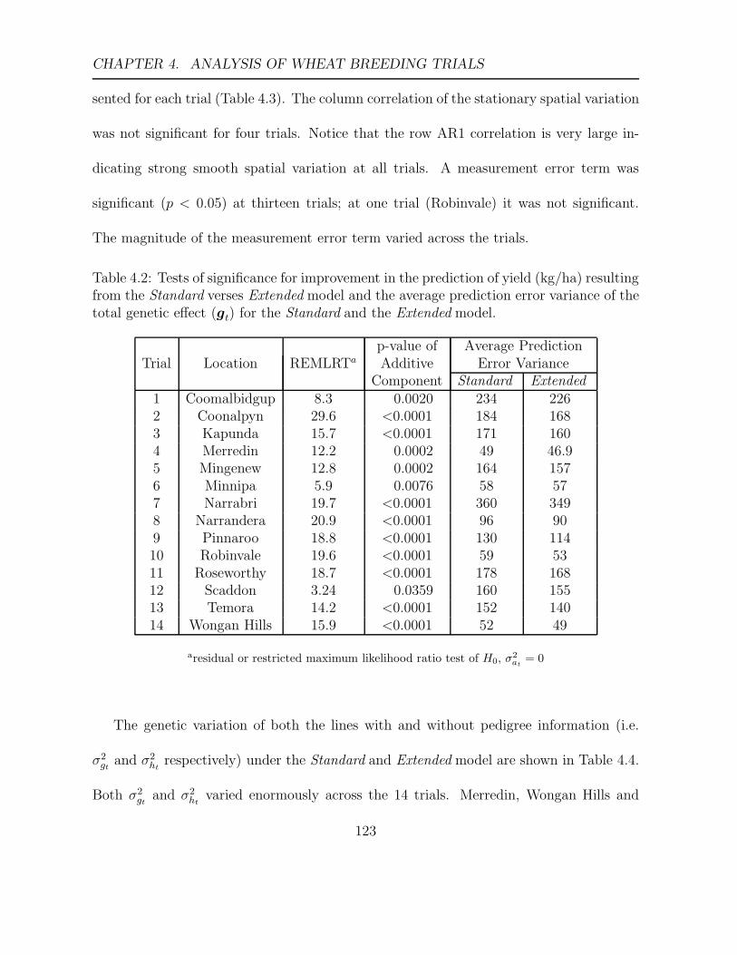
CHAPTER 4. ANALYSIS OF WHEAT BREEDING TRIALS
sented for each trial (Table 4.3). The column correlation of the stationary spatial variation
was not significant for four trials. Notice that the row AR1 correlation is very large in-
dicating strong smooth spatial variation at all trials. A measurement error term was
significant (p < 0.05) at thirteen trials; at one trial (Robinvale) it was not significant.
The magnitude of the measurement error term varied across the trials.
Table 4.2: Tests of significance for improvement in the prediction of yield (kg/ha) resultingfrom the Standard verses Extended model and the average prediction error variance of thetotal genetic effect (gt) for the Standard and the Extended model.
p-value of Average PredictionTrial Location REMLRTa Additive Error Variance
Component Standard Extended1 Coomalbidgup 8.3 0.0020 234 2262 Coonalpyn 29.6 <0.0001 184 1683 Kapunda 15.7 <0.0001 171 1604 Merredin 12.2 0.0002 49 46.95 Mingenew 12.8 0.0002 164 1576 Minnipa 5.9 0.0076 58 577 Narrabri 19.7 <0.0001 360 3498 Narrandera 20.9 <0.0001 96 909 Pinnaroo 18.8 <0.0001 130 11410 Robinvale 19.6 <0.0001 59 5311 Roseworthy 18.7 <0.0001 178 16812 Scaddon 3.24 0.0359 160 15513 Temora 14.2 <0.0001 152 14014 Wongan Hills 15.9 <0.0001 52 49
aresidual or restricted maximum likelihood ratio test of H0, σ2at
= 0
The genetic variation of both the lines with and without pedigree information (i.e.
σ2gt
and σ2ht
respectively) under the Standard and Extended model are shown in Table 4.4.
Both σ2gt
and σ2ht
varied enormously across the 14 trials. Merredin, Wongan Hills and
123
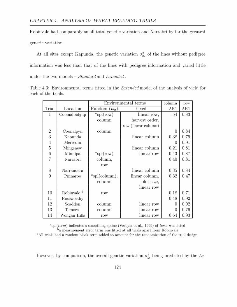
CHAPTER 4. ANALYSIS OF WHEAT BREEDING TRIALS
Robinvale had comparably small total genetic variation and Narrabri by far the greatest
genetic variation.
At all sites except Kapunda, the genetic variation σ2ht
of the lines without pedigree
information was less than that of the lines with pedigree information and varied little
under the two models – Standard and Extended .
Table 4.3: Environmental terms fitted in the Extended model of the analysis of yield foreach of the trials.
Environmental terms column row
Trial Location Random (uit) Fixed AR1 AR1
1 Coomalbidgup aspl(row) linear row, .54 0.83column harvest order,
row:(linear column)
2 Coonalpyn column 0 0.843 Kapunda linear column 0.38 0.794 Merredin 0 0.915 Mingenew linear column 0.21 0.816 Minnipa aspl(row) linear row 0.43 0.877 Narrabri column, 0.40 0.81
row8 Narrandera linear column 0.35 0.849 Pinnaroo aspl(column), linear column, 0.32 0.47
column plot size,linear row
10 Robinvale b row 0.18 0.7111 Roseworthy 0.48 0.9212 Scaddon column linear row 0 0.9213 Temora column linear row 0 0.7914 Wongan Hills row linear row 0.64 0.93
aspl(term) indicates a smoothing spline (Verbyla et al., 1999) of term was fittedba measurement error term was fitted at all trials apart from Robinvale
cAll trials had a random block term added to account for the randomization of the trial design.
However, by comparison, the overall genetic variation σ2gt
being predicted by the Ex-
124

CHAPTER 4. ANALYSIS OF WHEAT BREEDING TRIALS
tended model was higher than under the Standard model (Table 4.4). In some trials the
difference was substantial.
Table 4.4: The Total or overall genetic variance of yield (kg/ha) for lines with pedigree in-formation (σ2
gt) and lines without pedigree (σ2
ht) at each of the trials from the Standard and
Extended models and broad (H2) and narrow (h2) sense heritabilityb
Standard model Extended modelTrial Location aPercent
σ2ht
σ2gt
H2 σ2ht
σ2gt
Additive H2 h2
1 Coomalbidgup 71.44 90.26 0.69 70.58 110.29 77.08 0.64 0.422 Coonalpyn 57.97 59.91 0.71 59.78 68.20 100.00 c 0.60 0.603 Kapunda 35.06 19.06 0.24 39.65 26.15 100.00 c 0.22 0.224 Merredin 1.00 2.27 0.47 0.98 2.38 52.66 0.43 0.185 Mingenew 28.74 45.67 0.70 28.85 55.05 81.30 0.64 0.456 Minnipa 7.26 8.89 0.81 7.23 9.96 63.12 0.77 0.387 Narrabri 249.73 375.34 0.82 249.33 441.82 81.36 0.77 0.548 Narrandera 8.66 17.33 0.73 8.70 23.82 100.00 c 0.66 0.669 Pinnaroo 1.55 14.12 0.40 2.20 16.12 100.00 c 0.32 0.3210 Robinvale 2.87 4.23 0.58 3.11 4.68 92.65 0.48 0.4211 Roseworthy 42.50 55.45 0.71 42.49 60.31 76.10 0.64 0.4112 Scaddon 29.32 29.32 0.56 28.76 37.88 77.95 0.53 0.3513 Temora 17.20 22.18 0.47 17.73 29.58 100.00 c0.41 0.4114 Wongan Hills 2.99 3.81 0.64 3.07 5.17 100.00 c0.56 0.56
aadditive genetic variation as a percent of the total or overall genetic variation (σ2gt
) of theExtended model
bcalculated using the generalized heritability formula (3.6.30)cthe REML estimate of the epistatic genetic variance component was on the boundary at these trials,
therefore H2 and h2 are equivalent.
For the Extended model, the proportion of the total genetic variation represented by
the additive component varied across trials. At six trials, all the genetic variation was
found to be additive. The REML estimate of the epistatic variance at these trials was
zero.
125
CHAPTER 4. ANALYSIS OF WHEAT BREEDING TRIALS
The broad sense heritability of the Standard model was higher than the Extended model
(Table 4.4). This higher heritability is likely to be the result of an upward bias as a result
of an incorrect model (Costa e Silva et al., 2004). The narrow sense heritability which
is able to be determined under the Extended model is a more appropriate indicator of
heritability (Viana, 2005) and as such is the preferable indicator. Notice that Kapunda
has a low heritability.
There were high correlations between the overall total genetic E-BLUPs of the Stan-
dard (gt) and the Extended model (gt = at + it) (Table 4.5). This agreement was reflected
in terms of the top 20 ranking lines. However, across all trials there were differences in
the ranking of the lines in the top 20 lines. In particular, when the ranking of the top 20
lines was considered, on average across the sites four of the selections are different under
the two models (Figure 4.1).
In trials, where the epistatic component of the genetic variation was significant, the
correlations between the genetic E-BLUPs of the Standard (gt) and the additive genetic
E-BLUPs of the Extended model (at) were lower (Table 4.5), than when comparing the cor-
relation between the overall total genetic E-BLUPs of the Standard and Extended model.
However, the lower correlations do not reflect the differences in the top 20 ranking lines
under the two models. If decisions on the best potential parents were based on the pre-
dicted yield under the Standard model rather than on the additive predicted yield of the
Extended model then thirty percent of these decisions would be wrong (Figure 4.2).
126

CHAPTER 4. ANALYSIS OF WHEAT BREEDING TRIALS
Table 4.5: The correlations between the E-BLUPs of gt from the Standard model and theE-BLUPs gt = at + it and at respectively from Extended model
Trial Location aCorrelation(gt, at + it) (gt, at)
1 Coomalbidgup 0.986 0.9342 Coonalpyn 0.971 0.9713 Kapunda 0.813 0.8134 Merredin 0.961 0.7675 Mingenew 0.984 0.9406 Minnipa 0.996 0.9117 Narrabri 0.993 0.9588 Narrandera 0.982 0.9829 Pinnaroo 0.872 0.87210 Robinvale 0.944 0.92111 Roseworthy 0.982 0.91812 Scaddon 0.977 0.92413 Temora 0.930 0.9314 Wongan Hills 0.966 0.966
agt is the E-BLUP of gt from the Standard model and at and it are the E-BLUPs of at and it
respectively from the Extended model
On comparing Figures 4.1 and 4.2 the greater improvement in agreement between
models shown in Figure 4.1 particularly at Merredin, Roseworthy, Scaddon and Minnipa
is due to the inclusion of the epistatic component in the total genetic variation. Kapunda
and Pinnaroo both have 100% additive variation (i.e. no epistatic variation) and are
therefore unchanged across these trials. The lack of agreement between the two models
generally at these two trials may be due to their low heritability.
127

CH
AP
TE
R4.
AN
ALY
SIS
OF
WH
EAT
BR
EE
DIN
GT
RIA
LS
2400
2600
2800
3000
3200
3400
3600
Coomalbidgup
2400 2800 3200 3600
1600
1800
2000
2200
2400
Coonalpyn
1600 1800 2000 2200 2400
2800
2900
3000
3100
3200
3300
Kapunda
2900 3000 3100 3200
700
750
800
850 Merredin
700 750 800 850
1800
2000
2200
2400
2600
Mingenew
1800 2000 2200 2400 2600
600
700
800
900
1000
Minnipa
600 700 800 900 1000
4000
4500
5000
5500
6000
6500
Narrabri
4000 4500 5000 5500 6000 6500
700
800
900
1000
1100
1200
1300
Nerrandera
700 900 1100 1300
1600
1700
1800
1900
2000
Pinnaroo
1600 1700 1800 1900 2000
500
550
600
650
700
750
Robinvale
500 550 600 650 700 750
3000
3200
3400
3600
3800
4000
Roseworthy
3000 3200 3400 3600 3800 4000
2700
2800
2900
3000
3100
3200
Scaddon
2700 2900 3100
2100
2200
2300
2400
2500
2600
Temora
2100 2300 2500 2700
750
800
850
900
950
1000
Wongan Hills
800.0000 899.9965 999.9931
Standard model: predicted yield (kg/ha)
Exte
nded
mod
el: p
redi
cted
yie
ld (k
g/ha
)
Figure 4.1: The predicted (breeding value) yield (kg/ha) under the Extended model and the Standard model forlines with pedigree information. Horizontal and vertical lines show the cut off for the top 20 ranking lines underthe Extended and Standard model respectively. Each trial has been plotted on an individual scale, to enhance thepresentation.
128

CH
AP
TE
R4.
AN
ALY
SIS
OF
WH
EAT
BR
EE
DIN
GT
RIA
LS
2600
2800
3000
3200
3400
Coomalbidgup
2400 2800 3200 3600
1600
1800
2000
2200
2400
Coonalpyn
1600 1800 2000 2200 2400
2800
2900
3000
3100
3200
3300
Kapunda
2900 3000 3100 3200
740
760
780
800
Merredin
700 750 800 850
2000
2200
2400
2600
Mingenew
1800 2000 2200 2400 2600
650
700
750
800
850
900
Minnipa
600 700 800 900 1000
4500
5000
5500
6000
Narrabri
4000 4500 5000 5500 6000 6500
700
800
900
1000
1100
1200
1300
Nerrandera
700 900 1100 1300
1600
1700
1800
1900
2000
Pinnaroo
1600 1700 1800 1900 2000
630
635
640
645
650
Robinvale
500 550 600 650 700 750
3200
3400
3600
3800
Roseworthy
3000 3200 3400 3600 3800 4000
2800
2900
3000
3100
Scaddon
2700 2900 3100
2100
2200
2300
2400
2500
2600
Temora
2100 2300 2500 2700
750
800
850
900
950
1000
Wongan Hills
800.0000 899.9965 999.9931
Standard model: predicted yield (kg/ha)
Exte
nded
mod
el: A
dditi
ve p
redi
cted
yie
ld (k
g/ha
)
Figure 4.2: The additive predicted (breeding value) yield (kg/ha) for the Extended model plotted against the pre-dicted yield (kg/ha) of the Standard model for lines with pedigree information. Horizontal and vertical lines showthe cut off for the top 20 ranking lines under the Extended and Standard model respectively. Each trial has beenplotted on an individual scale, to enhance the presentation.
129

CHAPTER 4. ANALYSIS OF WHEAT BREEDING TRIALS
4.3 Multi-site analysis
4.3.1 Statistical Model
Multi-environment trial analyses were conducted. The single site analyses of Section 4.2
are a special case of a multi-environment trial analysis (Model 2, Table 4.6). The statis-
tical model fitted is
y = Xτ + Zgg + Zhh + Zuu + η
where y(n×1) is the full vector of yields of individual plots across each of p environment,
τ is a vector of fixed effects and includes overall or population means for the lines with
pedigrees, lines with unknown pedigree and the filler line, main effects for trials are fitted
as well as trial specific global or extraneous environmental terms. X is the corresponding
design matrix.
The vector g(mp×1) = (gT1 . . .g
Tp )T is the random genetic effects for the m lines with
known pedigree in each of the p trials. In the Extended model, g is partitioned into
the vectors of additive line effects a(mp×1) and epistatic line effects i(mp×1) such that the
Extended model has g = a + i, thus g ∼ N(0,Ga ⊗ A + Gi ⊗ Im), where A(m×m) is
the known additive relationship matrix defined by Eqn. 2.8.24. In the Standard model
the vector of total genetic effects for lines with known pedigree in each of the p trials is
g(mp×1) ∼ N(0,Gi ⊗ Im). The design matrix Z(n×mp)g associated with g, relates plots to
130
CHAPTER 4. ANALYSIS OF WHEAT BREEDING TRIALS
trial by line combinations.
The random vector u(c×1) consists of subvectors u(ci×1)i where the subvector ui corre-
sponds to the ith random term. The corresponding design matrix Z(n×c)u is partitioned
conformably as [Zu1 . . .Zuc]. The subvectors are assumed mutually independent with
variance σ2ui
Ici. The subvectors include random terms for extraneous field or environ-
mental variation specific to each environment such as random row or column variation
and design or randomization based blocking factors. For this example a random term for
blocks (replicates) is included for each trial.
The vector h(mhp×1) = (hT1 . . .h
Tp )T is the random genetic effects for the mh lines
without unknown pedigree in each of the p trials and h ∼ N(0,Gh ⊗ Imh). The design
matrix Z(n×mhp)h associated with h, relates plots to trial by line combinations.
The vector η(n×1) = (ηT1 . . .η
Tp )T consists of sub-vectors η
(nt×1)t representing local
stationary variation in the tth trial as described in Section 3.1.1.
The multi-environment analyses that follow were fitted in ASReml (Gilmour et al.,
2006).
4.3.2 Analysis
A summary of the the environmental or non-genetic components for each trial was pre-
sented in Table 4.3. In the multi-environment analyses that follow, the non-genetic terms
fitted were generally the same as those presented in Table 4.3, with refinement if nec-
131

CHAPTER 4. ANALYSIS OF WHEAT BREEDING TRIALS
essary. In particular, a measurement error term was unable to be fitted at any of the
trials in the multi-environment analyses that follows. Thus slightly inferior models were
fitted to the individual trials, which may result in the variance components being slightly
biased.
The multi-environment analyses fitted (Table 4.6) include several forms of the Stan-
dard and Extended models. The models were not necessarily nested so the goodness of
fit of models is compared using the Akaike Information Criterion (AIC, Akaike, 1974).
For each of the multi-environment analyses, the structure of the trial genetic variance
matrices Ga, Gi and Gh for each of the genetic components a, e and h respectively are
shown in Table 4.6. Many of the abbreviations for the variance structure are consistent
with ASReml syntax (Gilmour et al., 2006). The trial genetic variance matrix for the
lines with unknown pedigree are included because they differ between the models fitted.
Model 1 is the current approach to METs analysis used by AGT. Model 2 is equivalent to
fitting a separate analysis at each trial because it assumes a separate genetic variance for
each trial and no genetic covariance between pairs of trials. The results of the single site
analyses were discussed in detail in Section 4.2 and so are not referred to here in detail,
only as a comparison to the other models fitted. Models 1, 3 and 4 correspond to forms
of the Standard model. Model 1 has a compound symmetry structure for Gi (Patterson
et al., 1977) whereas Models 3 and 4 correspond to a factor analytic form of Gi of order
one and two respectively (Smith et al., 2001). Thus g the genetic vector for lines with
132

CHAPTER 4. ANALYSIS OF WHEAT BREEDING TRIALS
pedigree information is not partitioned in these models. Model 4 has a lower AIC than
Models 1 and 3 and therefore is the most appropriate of the Standard MET models fitted.
Table 4.6: Summary of models fitted showing the structure of the trial genetic variancematrices Ga, Gi and Gh for each of the genetic line effects a, i and h respectively.
Structure of trial genetic variance matrix REML LogModel Ga Gi Gd
h qb AICc Likelihood1 CS CS 67 969.64 -1477.112 DIAG DIAG (r) DIAG 105 448.42 -1178.503 - XFA1 XFA1 133 342.06 -1097.324e - XFA2 XFA1 147 243.54 -1034.065 CS CS CS 69 775.80 -1378.196 DIAG/CS DIAG/CS(r) DIAG/CS 116 124.02 -1005.307 XFA1 XFA1 (r) XFA1 149 82.40 -951.498a XFA2 XFA1 (r) XFA1 163 0.00 -896.29
a final Extended modelbq number of parameters in Ga, Gi and Gh fittedc AIC are relative to Model 8, so that positive values indicate the AIC is higher than Model 8d This is the structure of genetic variance component fitted to lines without pedigree informatione final Standard model
KEY
CS same genetic variance at each trial, same genetic covariance between pairs of trials (Patterson et al., 1977)
DIAG different genetic variance at each trial, no genetic covariance between pairs of trials, equivalent to fitting a singletrial analysis
DIAG/CS different genetic variance at each trial, same genetic covariance between pairs of trials (Cullis et al., 1998)
XFAF factor analytic with F factors (Smith et al., 2001)
(r) subset of trials 1, 4, 5, 6, 7, 10, 11, 12 fitted (note: if not specified all trials fitted)
AIC Akaike Information Criteria (Akaike, 1974)
The models are fitted in a hierarchial order so that the choice of models fitted further
down Table 4.6 may depend on the results of the previous models. In Model 2, the REML
estimates of the epistatic genetic variance components for six sites (Coonalpyn, Kapunda,
Narrandera, Pinnaroo, Temora and Wongan Hills) converged to zero (this was also shown
133

CHAPTER 4. ANALYSIS OF WHEAT BREEDING TRIALS
in Table 4.4). Models 6 through 8 therefore have structures for Gi that are fitted at a
reduced set of sites.
Models 5-8 are all MET analyses which use the Extended model for the total genetic
line effect, thus partitioning g into additive (a) and epistatic (i) genetic line effects. Thus
they are multi-environment extensions of the single trial analyses of Section 4.2. Notice
that the structure for the corresponding trial genetic variance matrices Ga and Gi are
not necessarily constrained to be equal. Model 5 is the Extended model of Patterson et al.
(1977) and shows the poorest performance of the Extended MET models. Model 6 is the
Extended model of Cullis et al. (1998). It allows a separate variance for each trial and has
a much lower AIC than Model 5 and the Standard model (Model 4, Table 4.6). Model 8
fits a factor analytic form for Ga of order two whereas model 7 fits a factor analytic form
of order one.
On comparing the AIC of the models fitted, Model 8 is the best performing model
(Table 4.6). It has the lowest AIC and therefore it is chosen as the most appropriate
Extended model and is referred to hereafter as the final model. The ASReml code for
Model 8 is shown in Appendix B.2. The results of the final model are now examined.
The REML estimates of the additive Ga and epistatic Gi genetic variance matrices
across each trial are summarised in Table 4.7. The REML estimates of the genetic variance
at each trials and the genetic correlations between pairs of trials are now examined. As
found in the single trial analyses the additive and epistatic genetic variance components
134

CHAPTER 4. ANALYSIS OF WHEAT BREEDING TRIALS
differ in magnitude between trials.
Additive genetic variance matrix Ga
To help interpret the additive genetic relationship between trials a biplot (Gabriel, 1971
and Smith et al., 2001) of the loadings of the first factor against the loadings of the
second factor for the additive genetic line effect a is shown in Figure 4.3. Merredin,
Minnipa, Narrandera and Robinvale form a group of trials which are strongly positively
correlated. Narrabri, Wongan Hills, Kapunda, Coomalbidgup, Scaddon, Pinnaroo, Rose-
worthy, Coonalpyn and Temora form a second group of positively correlated trials with
Scaddon, Pinnaroo and Roseworthy being particularly strongly positively correlated. Min-
genew is negatively correlated with the Merredin, Robinvale, Minnipa and Narrandera
trials, with little or no correlation with the other trials. In summary, for additive ge-
netic variation, the trial Mingenew appears to be different while the other trials form two
separate groups, within trials within each group performing similarly.
Epistatic genetic variance matrix Gi
For the epistatic component, trials Coomalbidgup, Robinvale, and Scaddon have very dif-
ferent estimated epistatic genetic variation but have perfect positive estimated correlation
with each other. Minnipa and Narrabri both have negligible or low correlation with other
trials.
135

CH
AP
TE
R4.
AN
ALY
SIS
OF
WH
EAT
BR
EE
DIN
GT
RIA
LS
Table 4.7: REML estimate of the components of the additive and epistatic genetic variance matricesa for yield(kg/ha) at each trials, in the final Extended model (Model 8, Table 4.6)
Ga 1 2 3 4 5 6 7 8 9 10 11 12 13 14Coomalbidgup 1 49918 0.36 0.33 0.18 0.16 0.07 0.26 0.00 0.47 0.14 0.43 0.52 0.43 0.28
Coonalpyn 2 76150 0.44 0.36 0.06 0.24 0.40 0.19 0.58 0.31 0.54 0.66 0.51 0.40Kapunda 3 32768 0.41 -0.02 0.31 0.43 0.28 0.56 0.37 0.52 0.64 0.48 0.41Merredin 4 3868 -0.44 0.69 0.56 0.75 0.42 0.69 0.42 0.53 0.29 0.48Mingenew 5 49440 -0.53 -0.23 -0.65 0.10 -0.46 0.06 0.07 0.19 -0.13Minnipa 6 11223 0.50 0.80 0.28 0.69 0.29 0.36 0.14 0.40Narrabri 7 363976 0.51 0.50 0.53 0.48 0.59 0.39 0.45
Narrandera 8 27147 0.21 0.76 0.23 0.30 0.06 0.40Pinnaroo 9 20441 0.37 0.68 0.84 0.66 0.50Robinvale 10 5421 0.37 0.46 0.23 0.44
Roseworthy 11 65884 0.78 0.60 0.47Scaddon 12 13384 0.74 0.59Temora 13 29376 0.41
Wongan Hills 14 5776
Gi 1 4 5 6 7 10 11 12Coomalbidgup 1 49337 -0.28 0.37 -0.01 -0.03 1.00 0.30 1.00
Merredin 4 55 -0.10 0.00 0.01 -0.28 -0.08 -0.28Mingenew 5 11524 0.00 -0.01 0.37 0.11 0.37Minnipa 6 1235 0.00 -0.01 0.00 -0.01Narrabri 7 100520 -0.03 -0.01 -0.03Robinvale 10 220 0.30 1.00
Roseworthy 11 9050 0.30Scaddon 12 24840
athese matrices are symmetric therefore only the upper triangle is shown, the diagonal elements of these matrices are genetic variancecomponents of each trial and the off-diagonal elements are genetic correlations between pairs of trials.
136
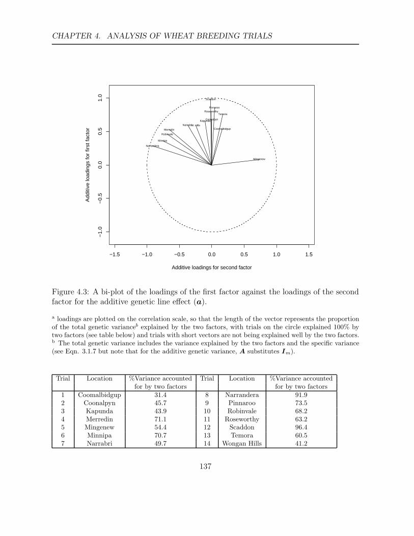
CHAPTER 4. ANALYSIS OF WHEAT BREEDING TRIALS
−1.5 −1.0 −0.5 0.0 0.5 1.0 1.5
−1.
0−
0.5
0.0
0.5
1.0
Additive loadings for second factor
Add
itive
load
ings
for
first
fact
or
CoonalpynKapunda
Mingenew
Merredin
Roseworthy
W. Hills
Scaddon
Temora
Narrabri
Pinnaroo
Coomalbidgup
Narrandera
Robinvale
Minnipa
Figure 4.3: A bi-plot of the loadings of the first factor against the loadings of the secondfactor for the additive genetic line effect (a).
a loadings are plotted on the correlation scale, so that the length of the vector represents the proportionof the total genetic varianceb explained by the two factors, with trials on the circle explained 100% bytwo factors (see table below) and trials with short vectors are not being explained well by the two factors.b The total genetic variance includes the variance explained by the two factors and the specific variance(see Eqn. 3.1.7 but note that for the additive genetic variance, A substitutes Im).
Trial Location %Variance accounted Trial Location %Variance accountedfor by two factors for by two factors
1 Coomalbidgup 31.4 8 Narrandera 91.92 Coonalpyn 45.7 9 Pinnaroo 73.53 Kapunda 43.9 10 Robinvale 68.24 Merredin 71.1 11 Roseworthy 63.25 Mingenew 54.4 12 Scaddon 96.46 Minnipa 70.7 13 Temora 60.57 Narrabri 49.7 14 Wongan Hills 41.2
137

CHAPTER 4. ANALYSIS OF WHEAT BREEDING TRIALS
The total genetic variance at a particular trial is approximated by the sum of the
epistatic genetic variance and the additive genetic variance given by the REML estimate
of the diagonal elements of Gi plus the the REML estimate of the diagonal elements of
Ga multiplied by the average of the diagonal element of A and is given in Table 4.8. Note:
for this example as all the lines are assumed completely homozygous – the average is 2
Table 4.8: Summary of the REML estimates of the total genetic variance and percentadditive and epistatic variance in yield (t/ha) for lines with pedigree information at thefinal model (Model 8, Table 4.6).
Trial Location %var(a) %var(i) var(g)a
1 Coomalbidgup 66.9 33.1 1492 Coonalpyn 100.0 0.0 1523 Kapunda 100.0 0.0 664 Merredin 99.3 0.7 85 Mingenew 89.6 10.4 1106 Minnipa 94.8 5.2 247 Narrabri 87.9 12.1 8288 Narrandera 100.0 0.0 549 Pinnaroo 100.0 0.0 4110 Robinvale 98.0 2.0 1111 Roseworthy 93.6 6.4 14112 Scaddon 51.9 48.1 5213 Temora 100.0 0.0 5914 Wongan Hills 100.0 0.0 12
avar(g)=var(a)+var(i), where var(a) is the diagonal elements of the REML estimates of Ga (Table4.7), multiplied by the average of the diagonal elements of A (i.e. 2) and var(i) is the diagonal elements
of the REML estimates of Gi, (Table 4.7).
The total genetic variance in yield of lines with pedigree information accounted for
under the Extended MET analysis (Table 4.8) is much greater than under the single trial
analyses (Table 4.4). There were eight trials that had the percentage of additive variation
138

CHAPTER 4. ANALYSIS OF WHEAT BREEDING TRIALS
less than 100%. At six of these trials, the percentage of additive variation increased
dramatically in the MET compared to single trial analyses. However, at two of these
trials, namely, Scaddon and Coomalbidgup the percentage of additive variation decreased.
Predictions of genetic line effects for individual trials can be used to form an appropriately
weighted selection index for each of the genetic components (Section 3.5). In order to
compare models in the most efficient way, the fourteen trials were given equal weights in
each selection index as in Kelly et al. (2007). Other appropriate selection indices could
be calculated, for instance selection indices of trials which performed similarly could be
evaluated. Section 3.5 provides a more detailed discussion of possible selection indices.
The following figures show only lines with known pedigree as these are the lines of most
interest.
A high correlation (0.996) between the predicted selection indices for the total genetic
effects of the Standard model (Model 4, Table 4.6) and the final model (Model 8, Table 4.6)
was apparent (Figure 4.4). However, in comparison to the final model the Standard model
generally under-estimates the additive selection index values. The top three ranking lines
were the same under both models. However, there were important differences in the
ranking of other lines between the two models. In particular, when the ranking of the top
20 lines was considered, two of the selections are different under the two models.
A high positive correlation (0.96) was found between the predicted total genetic selec-
tion index of the Standard model (Model 4, Table 4.6) and the additive genetic predicted
139
CHAPTER 4. ANALYSIS OF WHEAT BREEDING TRIALS
selection index of the final model (Figure 4.5). The top three ranking lines were the same
under both models. However, there were differences in the ranking of the other lines in
the top 20. In particular, when the ranking of the top 20 lines was considered, four of
the selections are different under the two models. These results are consistent with those
found under the single trial analyses.
Finally, the total selection index of yield (kg/ha) for the final model (Model 8, Table
4.6) is compared to the total selection index of the current model used by AGT (Model
1, Table 4.6)(Figure 4.6). In comparison to the final model the model fitted by AGT gen-
erally over-estimates the total selection index values for higher yields and underestimates
the total selection index for lower yields. There were also important differences in the
ranking of the lines between the two models. For example, the top 3 ranking lines under
Model 1 are ranked 3rd, 11th and 63rd respectively under the final model and the top 3
ranking line under the final model were ranked 4th, 26th and 1st respectively under the
AGT model. In addition, when the ranking of the top 20 lines is considered, 7 of the
selections are different under the two models.
140

CHAPTER 4. ANALYSIS OF WHEAT BREEDING TRIALS
Standard model: Total Selection Index
Fina
l mod
el: T
otal
Sel
ectio
n In
dex
−300
−200
−100
010
020
0
−300 −200 −100 0 100 200
Figure 4.4: The predicted total selection index of the Standard model (Model 4, Table
4.6) plotted against the predicted total selection index of yield (kg/ha) for the final model
(Model 8, Table 4.6). The straight line is the line of equivalence(y=x).
141
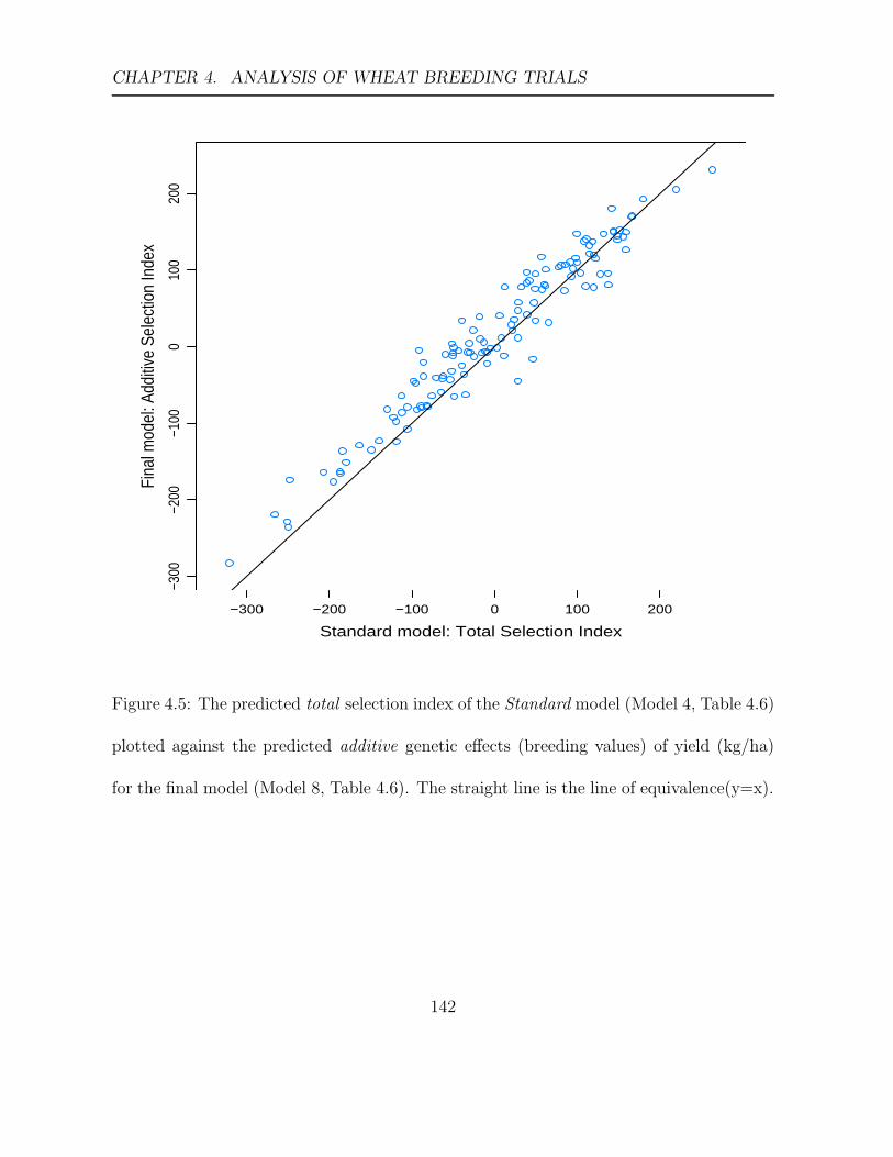
CHAPTER 4. ANALYSIS OF WHEAT BREEDING TRIALS
Standard model: Total Selection Index
Fina
l mod
el: A
dditi
ve S
elec
tion
Inde
x−3
00−2
00−1
000
100
200
−300 −200 −100 0 100 200
Figure 4.5: The predicted total selection index of the Standard model (Model 4, Table 4.6)
plotted against the predicted additive genetic effects (breeding values) of yield (kg/ha)
for the final model (Model 8, Table 4.6). The straight line is the line of equivalence(y=x).
142

CHAPTER 4. ANALYSIS OF WHEAT BREEDING TRIALS
Model 1: Total Selection Index
Fina
l mod
el: T
otal
Sel
ectio
n In
dex
−300
−200
−100
010
020
0
−200 −100 0 100
Figure 4.6: The predicted total selection index of Model 1 (Table 4.6) plotted against the
predicted total selection index of yield (kg/ha) for the final model (Model 8, Table 4.6).
The straight line is the line of equivalence(y=x).
143

Chapter 5
Analysis of Sugarcane Breeding
Trials
The multi-environment trial example considered in this chapter is from the joint sugar-
cane breeding program of BSES Ltd and the Commonwealth Scientific Industrial Research
Organisation (CSIRO) and was kindly provided by Xianming Wei. The aims of the joint
sugarcane breeding program are similar to those of the AGT wheat breeding program dis-
cussed in Chapter 4. However, an additional aim in the sugarcane breeding program is to
determine the parental crosses which result in superior hybrid clones. Multi-environment
trials are conducted by the joint breeding program to assess the overall performance of
clones across environments. The program uses the approach of Smith et al. (2001) for
the analysis of multi-environment trials, these types of models have been fitted here as a
144

CHAPTER 5. ANALYSIS OF SUGARCANE BREEDING TRIALS
comparison (Models 1 and 2, Table 5.3).
The sugarcane clones tested in the annual breeding trial program are the result of a F1
(1st filial generation) cross between inbred parental lines and the clones are therefore hy-
brids. Thus the methodology developed in Chapters 2 and 3 for hybrid lines is illustrated
in this chapter.
5.1 Trial Details
A large number of clones were evaluated (and selected) in 2002 at two environments in
South East Queensland in ‘Stage 2’ or Clonal Assessment Trials (CATs). These trials in-
volved clones planted in a single 10m plot, interspersed with multiple plots of (the same) 4
commercial varieties in a grid-plot layout. Land availability at the environments governed
the spatial layout configuration and resulted in two contiguous row by column arrays of
plots at the MQN trial. A selected set of 80 clones from these CATs were then planted
in four ‘Stage 3’ or Final Assessment Trials (FATs) in 2003. Each FAT was designed
as a latinized row-column design (John et al., 2002) with 2 replicates (and included ad-
ditional plots of 25 commercial clones) using the software CycDesigN (Whitaker et al.,
2006). Again land availability at each environment necessitated 2 contiguous arrays or
subtrials. Plots were 4 rows by 10m with data recorded from the middle 2 rows to reduce
competition. Hereafter clones are synonymous with lines. In summary, there were 2242
unique lines tested across both the CATs, with 80 of these included in the FATs along
145

CHAPTER 5. ANALYSIS OF SUGARCANE BREEDING TRIALS
side 25 additional commercial varieties. Table 5.1 presents a summary of information for
each trial including the design layout. Thus in total the data consist of six trials made
up of 11 subtrials.
Table 5.1: Summary of the design layout and other details of the sugar example subtrials.
Year Trial Typea Linesb Mean CCSc,% Subtrial Columns Rows Plotsd
2002 BIN1 CAT 1236 11.37 1 30 46 1380
2002 MQN CAT 1010 14.29 2 16 58 1144
3 8 27
2003 BIN2 FAT 105 13.52 4 14 8 224
5 14 8
2003 FMD FAT 105 16.22 6 16 7 224
7 16 7
2003 ISS FAT 105 13.98 8 14 8 224
9 14 8
2003 MYB FAT 105 13.73 10 16 7 224
11 16 7
aCAT: clonal assessment trial, FAT: final assessment trialbNumber of lines planted for each trial (across subtrials)
cCCS (Commercial Cane Sugar)dTotal plots for each trial (across subtrials)
The pedigree of all of the lines in the CATs and FATs and their parents was available
146
CHAPTER 5. ANALYSIS OF SUGARCANE BREEDING TRIALS
resulting in pedigree information on 2663 lines, going back several generations. The data
considered are from plant cane measures of commercial cane sugar (CCS, %). CCS is
an industry formula and estimates the percentage of recoverable sucrose in the cane on a
fresh weight basis (BSES, 1984).
5.2 Statistical Model
Multi-environment trial analyses are fitted which include the single site analyses as a
special case (Model 4, Table 4.6). The statistical model is
y = Xτ + Zgg + Zuu + η
where y(n×1) is the full vector of CCS% of individual plots across each of p environments
(synonymous with trials), τ is the vector of fixed terms and includes an overall mean
performance for each trial as well as sub-trial specific global or extraneous environmental
terms, X is the corresponding design matrix, g(mp×1) = (gT1 , . . . , g
Tp )T is the vector of
random genetic effects of the m lines in each of p sites. In the Extended model the
vector g is partitioned into vectors of additive line effects a(mp×1), dominance line effects
d(mp×1) and residual non-additive line effects i(mp×1) such that the Extended model has
g = a + d + i.
The vector d can be partitioned such that d = Zbdb + dw, where d(vp×1)b is a vector
of dominance effects relating to between family effects, where v is the number of families,
with corresponding design matrix Z(mp×vp)b and d(mp×1)
w is a vector of dominance effects
147

CHAPTER 5. ANALYSIS OF SUGARCANE BREEDING TRIALS
relating to within family line effects. For this example across the six sites there are
m=2267 lines from v=193 families. By partitioning d, the calculation of the dominance
relationships between lines was reduced at least 122-fold from a potential maximum of
2570778 data points to a potential maximum of 20988 data points. In addition, there are
considerable reductions in the calculation of dominance relationships between ancestral
gamete pairs when the family pedigree rather than the full pedigree is used (Section 3.3);
this is because there are fewer ancestral gamete pairs. Thus g ∼ N(0,Ga ⊗ A + Gd ⊗
(ZbDbZTb + Dw) + Gi ⊗ Im), where A(m×m) is the known additive relationship matrix
defined by Eqn. 2.8.24, D(v×v)b is the known between family dominance relationship
matrix and D(m×m)w is the known within family dominance line matrix. Both of the
latter matrices are defined in Section 3.3. In the Standard model the random vector of
total genetic effects for m lines in each of the p trials g(mp×1), is not partitioned and
g ∼ N(0,Gi ⊗ Im). The design matrix Z(n×mp)g associated with g, relates plots to trial
by line combinations.
u(c×1) is the vector of random effects for extraneous environmental variation specific
to each sub-trial, and design or randomization based blocking factors (Cullis et al., 2007).
For this example randomization based blocking factors include trial by sub-trial and a
block (replicate) effect at each trial, Z(n×c)u is its associated design matrix.
As in the previous analyses, the vector η(n×1) = (ηT1 , . . . ,η
Tp )T consists of sub-vectors
η(nt×1)t representing local stationary variation in the tth subtrial as described in Section
148
CHAPTER 5. ANALYSIS OF SUGARCANE BREEDING TRIALS
3.1.1. Again, the software package ASReml (Gilmour et al., 2006) was used to fit the
models.
5.3 Analysis
The multi-environment analyses fitted (Table 5.3) include several forms of the Stan-
dard and Extended models. As in Chapter 4 the models were not necessarily nested so
the goodness of fit of models is compared using the Akaike Information Criterion (AIC,
Akaike, 1974). A summary of the models chosen to account for the non-genetic compo-
nent of the data is presented in Table 5.2. The REML estimates of the spatial correlations
(AR1 parameters) for columns and rows respectively are from the final Extended model
(Model 11, Table 5.3). In all of the models fitted these same environmental or non-genetic
terms were included. Blocking or randomisation terms fitted but not shown in this table
included a trial by subtrial effect and a replicate effect at each trial.
For each of the multi-environment analyses, the structure of the trial variance matrices
Ga, Gd and Gi for the genetic components a, d and i respectively is shown in Table 5.3.
Models 3 and 4 are equivalent to fitting a separate analysis at each trial because they
assume a separate genetic variance for each trial and no genetic covariance between pairs
of trials. Model 3 partitions the genetic line effect into an additive and a general non-
additive genetic effect. Model 4 further partitions the non-additive genetic effect into
dominance and residual non-additive effects. Model 4 is more appropriate here because
149

CHAPTER 5. ANALYSIS OF SUGARCANE BREEDING TRIALS
the clones are F1 hybrids in contrast to the wheat example in Chapter 4, where lines were
inbred and homozygous with the dominance effect assumed zero.
Table 5.2: Non-genetic terms (excluding blocking termsb) used in the MET analysis ofthe sugar example.
Environmental Terms acolumn arow
Trial Subtrial Random Fixed AR1 AR1
BIN1 1 column, 0.09 0.15row
MQN 2 0.27 0.233 column 0.17 0.10
BIN2 4 lin(row), 0.59 0.52lin(column)
5 lin(row) 0.06 0FMD 6 0 0
7 0 0.14ISS 8 0.36 0.21
9 0.0 0.13MYB 10 0 0.33
11 row 0 0
acolumn and row correlations presented were from the final model (Model 11, Table 5.3).bBlocking terms fitted include subtrial and replicate effect at each trial
Thus the non-additive genetic effect can and should be partitioned. The remain-
ing models fitted are MET analyses. Models 1 and 2 correspond to forms of the Stan-
dard model where a factor analytic model of order one and two respectively have been
fitted. Thus g is not partitioned in models 1 and 2. Model 2 has a lower AIC than model
1 and therefore is the (final) Standard model. The non-genetic terms fitted at each trial
(Table 5.2) are determined from this model and then used when fitting further models,
with adjustment if necessary. The single trial analyses which partition the genetic line
150

CHAPTER 5. ANALYSIS OF SUGARCANE BREEDING TRIALS
effect into components (Models 3 and 4) provide a better fit (based on AIC) than the
Standard model (Model 2, Table 5.3). This is despite the fact that these models do not
allow for any genetic correlation between trials.
Model 5 (Table 5.3) provides only an additive genetic component (Crossa et al., 2006).
Model 6 is the multi-environment extension of the Pedigree model of Oakey et al. (2006).
Model 6 has a much lower AIC and is therefore a better fit than Model 5. Models 5
and 6 have been fitted for comparison purposes only and are not recommended as the
models of choice for F1-hybrid data. Model 6 is however appropriate if the data consist
solely of fully inbred lines as in Chapter 4 where the dominance component is assumed
to be zero. Models 7 – 11 are all MET analyses which use the Extended model for the
genetic line effect, but have different structures for the trial genetic variance matrices Ga,
Gd and Gi for each of the genetic component a, d and i respectively. Models 7 and 8
are the poorest performing Extended MET models. Model 7, is the Extended model of
Patterson et al. (1977) and Model 8 is the Extended model of Cullis et al. (1998). All of
the Extended MET models (excluding Model 7) are superior to Model 5 which fits only
additive genetic effects. As discussed in Section 3.4, the models (Table 5.3) are fitted in a
hierarchial order so that the choice of models fitted further down the Table may depend
on the results of the previous models. For example, Models 8 through 11 have structures
for Gd and Gi that are fitted at a reduced set of trials, because having examined Model
4, the REML estimates of some of the trial genetic variances of Gd or Gi converged to
151

CHAPTER 5. ANALYSIS OF SUGARCANE BREEDING TRIALS
zero. Specifically, for Gd, the genetic variances of two trials (MQN and MYB) converged
to zero and for Gi, the genetic variance of three trials (BIN2, FMD and ISS) converged
to zero.
Table 5.3: Summary of models fitted showing the structure of the trial genetic variancematrix for each of the genetic components.
Structure of trial genetic variance matrix REML LogModel Ga Gd Gi qb AICc Likelihood
1 - - XFA1 53 4263.36 -2469.242d - - XFA2 59 4258.14 -2460.823 DIAG - DIAG 53 4213.68 -2444.404 DIAG DIAG(1, 2, 3, 4, 5) DIAG (1, 2, 6) 55 4202.34 -2436.735 XFA1 - - 53 4137.22 -2406.176 XFA1 - XFA1 65 4108.20 -2379.667 CS CS CS 47 4149.60 -2418.528 DIAG/CS DIAG/CS (1, 2, 3, 4, 5) DIAG/CS (1, 2, 6) 58 4127.74 -2396.439 XFA1 DIAG/CS (1, 2, 3, 4, 5) DIAG/CS(1, 2, 6) 63 2206.18 -1430.6510 XFA1 XFA1 (1, 2, 3, 4, 5) XFA1 (1, 2, 6) 68 1092.71 -868.9211a XFA2 XFA1 (1, 2, 3, 4, 5) XFA1 (1, 2, 6) 73 0.00 -317.56
a Final Extended modelbq number of parameters in Ga and Gi fittedc AIC are relative to Model 11, so that positive values indicate the AIC is higher than Model 11d Final Standard model
KEY
CS same genetic variance at each trial, same genetic covariance between pairs of trials (Patterson et al., 1977)
DIAG different genetic variance at each trial, no genetic covariance between pairs of trials, equivalent to fitting a singletrial analysis
DIAG/CS different genetic variance at each trial, same genetic correlation between pairs of trials (Cullis et al., 1998)
XFAF factor analytic with F factors (Smith et al., 2001)
(trials) subset of trials fitted (note: if not specified all trials fitted)
AIC Akaike Information Criteria (Akaike, 1974)
On comparing the AIC of the models fitted, Models 9, 10 and 11 are the best per-
forming models (Table 5.3). However, Model 11 has the lowest AIC and therefore it is
152

CHAPTER 5. ANALYSIS OF SUGARCANE BREEDING TRIALS
chosen as the most appropriate and final model. The results of the final model are now
examined. The REML estimates of the additive, dominance and residual non-additive
genetic variance matrices for trials are summarised in Table 5.4
The REML estimates of the genetic variances of trials and the correlations between tri-
als are now examined. Firstly, the additive, dominance and residual non-additive genetic
variance components differ in magnitude between trials.
For the additive component, a bi-plot (Gabriel, 1971 and Smith et al., 2001) of the
loadings of the first factor against the loadings of the second factor for the additive
genetic line effect a of the final model (Model 11, Table 5.3) is shown in Figure 5.1 to
help with the interpretation. A strong positive estimated correlation exists between five
of the six trials (Table 5.4). FMD was the exception and shows reduced correlations with
all other trials except MYB. For the dominance component, a strong positive estimated
correlation exists between four of the five trials; again FMD was the exception showing
reduced correlations. For the residual non-additive component, the correlation between
MYB and the other trials is negative. In summary, where genetic variation existed at
the additive, dominance and residual non-additive levels, the trial FMD appears to be
different while the other trials tend to perform similarly. This trial appeared to have a
much lower total genetic variance (var(g), Table 5.5) than other trials.
153
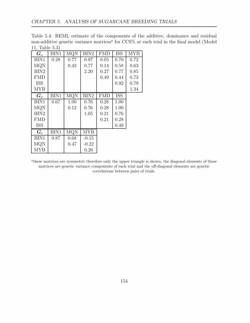
CHAPTER 5. ANALYSIS OF SUGARCANE BREEDING TRIALS
Table 5.4: REML estimate of the components of the additive, dominance and residualnon-additive genetic variance matricesa for CCS% at each trial in the final model (Model11, Table 5.3)
Ga BIN1 MQN BIN2 FMD ISS MYBBIN1 0.28 0.77 0.97 0.05 0.70 0.72MQN 0.43 0.77 0.14 0.58 0.63BIN2 2.20 0.27 0.77 0.85FMD 0.49 0.44 0.73ISS 0.92 0.79
MYB 1.34
Gd BIN1 MQN BIN2 FMD ISSBIN1 0.67 1.00 0.76 0.28 1.00MQN 0.12 0.76 0.28 1.00BIN2 1.05 0.21 0.76FMD 0.21 0.28ISS 0.49
Gi BIN1 MQN MYBBIN1 0.87 0.68 -0.15MQN 0.47 -0.22MYB 0.26
athese matrices are symmetric therefore only the upper triangle is shown, the diagonal elements of thesematrices are genetic variance components of each trial and the off-diagonal elements are genetic
correlations between pairs of trials.
154

CHAPTER 5. ANALYSIS OF SUGARCANE BREEDING TRIALS
−1.0 −0.5 0.0 0.5 1.0
−1.
0−
0.5
0.0
0.5
1.0
Additive loadings for second factor
Add
itive
load
ings
for
first
fact
or
BIN2
BIN1
FMD
ISS
MQN
MYB
Figure 5.1: A bi-plot of the loadings of the first factor against the loadings of the secondfactor for the additive genetic line effect a.
a loadings are plotted on the correlation scale, so that the length of the vector represents the proportionof the total genetic varianceb explained by the two factors, with trials on the circle explained 100% bytwo factors (see table below) and trials with short vectors are not being explained well by the two factors.b The total genetic variance includes the variance explained by the two factors and the specific variance(see Eqn. 3.1.7 but note that for the additive genetic variance A, substitutes Im).
Location %Variance accountedfor by two factors
BIN1 100MQN 82.1BIN2 96.6ISS 67.1
FMD 100MYB 100
155

CHAPTER 5. ANALYSIS OF SUGARCANE BREEDING TRIALS
The total variance at a particular trial is approximated by the sum of the residual
non-additive, dominance and the additive genetic variance given by the REML estimate
of the diagonal elements of Gi plus the REML estimate of the diagonal elements of Ga
multiplied by the average of the diagonal element of A plus the REML estimate of the
diagonal elements of Gd multiplied by the average of the diagonal element of D, where the
REML estimates of the additive variance Ga, dominance genetic variance D and residual
non-additive variance Gi of each trial were shown as the diagonal elements in Table 5.4.
Table 5.5: Summary of the REML estimates of the total genetic variance and percent
additive, dominance and epistatic variance in CCS for the final model (Model 11, Table
5.3, page 152)
Trial Typeb %var(a) %var(d) %var(i) var(g)
BIN1 CAT 16.7 35.0 48.3 1.809
MQN CAT 44.4 10.4 45.2 1.040
BIN2 FAT 70.3 29.7 0.0 3.330
FMD FAT 72.4 27.6 0.0 0.725
ISS FAT 67.9 32.1 0.0 1.448
MYB FAT 84.5 0.0 15.5 1.682
athese are the sum of the REML estimates of Ga, Gd and Gi, shown as diagonal elements of Table 5.4,
with Ga and Gd being multiplied by the average of the diagonal elements of A and D respectively.
bFAT: final assessment trial, CAT: clonal assessment trial
156

CHAPTER 5. ANALYSIS OF SUGARCANE BREEDING TRIALS
At all the FAT trials, after selection has occurred, the non-additive component of
variance was composed of either dominance or residual non-additive variance. At the two
CAT trials both dominance and residual non-additive variance was estimable. If selection
was solely on the basis of CCS, then it may be expected that the genetic variance in
the FATs would be less than that observed in the CATs. However, selection to progress
clones from the FATs to the CATs was based on Net Merit Grade which is only weakly
associated with CCS. For the clonal trials (trial BIN1 and MQN) in particular, the non-
additive variance comprised a greater proportion of the total variance than at the other
trials. This would suggest that the FATs are the more appropriate trials to select the
best parents from as these have a much higher proportion of estimated additive genetic
variation than the CATs. Indeed, this is the current practice in BSES-CSIRO breeding
programs.
Predictions of genetic line effects for individual trials can be used to form an appropri-
ately weighted selection index for each of the genetic components (Section 3.5). In order
to compare models in the most efficient way, again, the six trials were given equal weights
in each selection index as in Kelly et al. (2007). Other appropriate selection indices could
be calculated, for instance selection indices of trials which performed similarly could be
evaluated. Section 3.5 provides a more detailed discussion of possible selection indices.
As the selection of FAT lines from the CATs has taken place, the following figures
(except Figure 5.2) show only those lines evaluated in FATs. Figure 5.2 was materially
157

CHAPTER 5. ANALYSIS OF SUGARCANE BREEDING TRIALS
different when excluding lines that had not been selected. The other figures are represen-
tative of the full results.
There is no obvious relationship between the dominance between family selection index
and the dominance within family line selection index (Figure 5.2). The performance of the
different families varies, however most families show a range of different line performances.
There is a weak correlation (0.45) between between the predicted additive selection
index and the (overall) predicted dominance selection index of the lines (Figure 5.3).
There is a cluster of lines that have high additive selection indices and high dominance
selection indices, so that breeders are able to choose lines with high values for both indices.
A high correlation (0.96) between the predicted selection indices for the total ge-
netic effects of the Standard model (Model 2, Table 5.3) and the final model (Model 11,
Table 5.3) was apparent (Figure 5.4). However, in comparison to the final model the
Standard model generally under-estimates the total selection indices values at the lower
selection index values and over estimates at the higher selection index values. There were
also important differences in the ranking of the lines between the two models. When the
ranking of the top 20 lines is considered, 2 of the selections are different under the two
models.
A positive correlation (0.77) was found between the predicted total genetic selection
index of the Standard model (Model 2, Table 5.3) and the additive genetic predicted
selection index of the final model (Figure 5.5). However, again, there were important
158

CHAPTER 5. ANALYSIS OF SUGARCANE BREEDING TRIALS
differences in the ranking of lines between the two models. For example, when the ranking
of the top 20 lines is considered, 6 of the selections are different under the two models.
The top ranking line under the final model was ranked 4th under the Standard model.
Dominance between family Selection Index
Dom
inan
ce w
ithin
fam
ily li
ne S
elec
tion
Inde
x
−0.5
0.0
0.5
−0.4 −0.2 0.0 0.2 0.4
Figure 5.2: The predicted dominance between family selection index plotted against the
predicted dominance with family line selection index of CCS for the final model (Model
11, Table 5.3).
159

CHAPTER 5. ANALYSIS OF SUGARCANE BREEDING TRIALS
Dominance Selection Index
Addi
tive
Sele
ctio
n In
dex
−0.5
0.0
0.5
1.0
1.5
−1.0 −0.5 0.0 0.5 1.0
Figure 5.3: The predicted additive selection index (breeding value index) plotted against
the predicted dominance selection index of CCS for the final model (Model 11, Table 5.3).
160
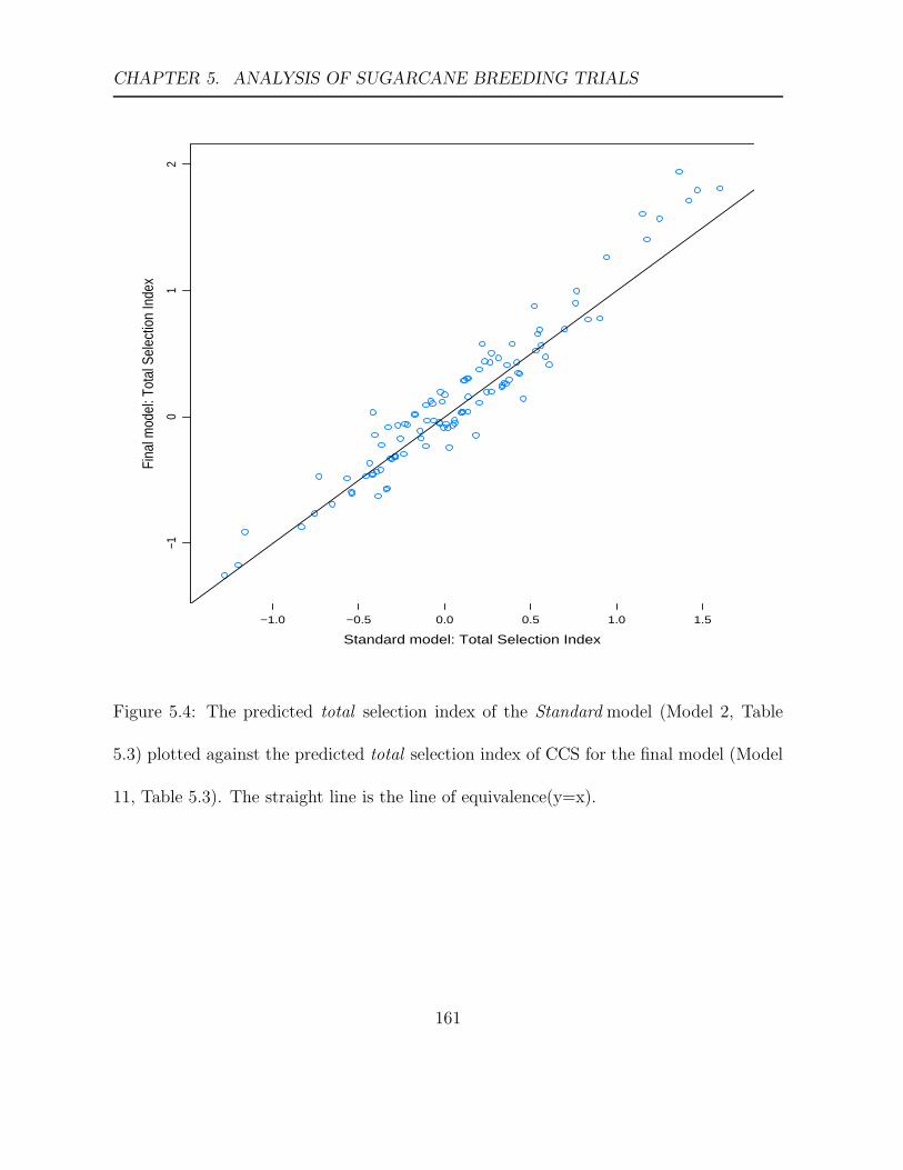
CHAPTER 5. ANALYSIS OF SUGARCANE BREEDING TRIALS
Standard model: Total Selection Index
Fina
l mod
el: T
otal
Sel
ectio
n In
dex
−10
12
−1.0 −0.5 0.0 0.5 1.0 1.5
Figure 5.4: The predicted total selection index of the Standard model (Model 2, Table
5.3) plotted against the predicted total selection index of CCS for the final model (Model
11, Table 5.3). The straight line is the line of equivalence(y=x).
161

CHAPTER 5. ANALYSIS OF SUGARCANE BREEDING TRIALS
Standard model: Total Selection Index
Fina
l mod
el: A
dditi
ve S
elec
tion
Inde
x
−0.5
0.0
0.5
1.0
1.5
−1.0 −0.5 0.0 0.5 1.0 1.5
Figure 5.5: The predicted total selection index of the Standard model (Model 2, Table
5.3) plotted against the predicted additive genetic effects (breeding values) of CCS for the
final model (Model 11, Table 5.3). The straight line is the line of equivalence(y=x).
162

CHAPTER 5. ANALYSIS OF SUGARCANE BREEDING TRIALS
5.4 Comparison of the results with the analysis pre-
sented by Oakey et al. (2007)
The sugarcane data set has been previously analysed and the results were presented in
the paper by Oakey et al. (2007). The method used to create the dominance matrix
by Oakey et al. (2007) was based on the theoretical result for dominance of Verbyla &
Oakey (2007). Verbyla & Oakey (2007) attempted to determine explicit expressions for the
identity mode probabilities of Table 2.1 in terms of the inbreeding coefficients of the lines
j and k and the coefficient of parentage between the lines j and k; the ultimate aim was
to obtain explicit expressions for the elements in the relationship matrices in Eqn. 2.7.23.
The theoretical results for determining the relationship matrices presented by Verbyla &
Oakey (2007) relied on an assumption of independence of identity by descent (IBD) events
in the determination of the identity probabilities. However, since the publication of Oakey
et al., 2007, it has been determined (through journal peer review) that the assumption of
independence is not valid. Therefore the dominance matrix used in Oakey et al. (2007)
is not the correct full dominance matrix as was represented in that paper.
For completeness, the results of the sugarcane data set analysis presented in the Oakey
et al. (2007) paper are now contrasted briefly with those shown in this Chapter. Oakey
et al. (2007) fitted the same structures for each genetic variance matrix as that shown
in Table 5.3. The final model chosen under Oakey et al. (2007) was a factor analytic
structure with two factors for the additive genetic variance matrix Ga, a separate factor
163

CHAPTER 5. ANALYSIS OF SUGARCANE BREEDING TRIALS
analytic structure with one factor for the dominance genetic variance matrix Gd and a
separate factor analytic structure with one factor for the residual non-additive variance
matrix Gi. Thus the final model fitted was similar to that of Model 11 (Table 5.3). The
main difference in the results of the analysis of Oakey et al. (2007), was that the dom-
inance genetic component of the site MQN was zero. Using the correct full dominance
matrix in the analysis (Section 5.3) of the sugarcane data set, allowed the full partitioning
of the genetic component in the MQN site, whereas the method in Oakey et al. (2007)
failed to estimate the dominance component for the MQN site. The correlations of the
genetic components of the MQN site with other sites were therefore effected as the pro-
portion of each of the genetic component estimated in the MQN site changed. It has been
established that the method of calculating dominance used in Oakey et al. (2007) is incor-
rect. However, for the sugarcane data set a comparison between the results of Section 5.3
and Oakey et al. (2007) suggest that the Oakey et al. (2007) method approximates the
true results, but with a loss of information. Clearly if the approach Oakey et al. (2007) is
to be used as an approximation of the true dominance matrix then further investigation
is required.
164

Chapter 6
Model performance under simulation
In this chapter simulation is used to investigate the performance of the Standard , Ad-
ditive and Extended models described in Chapter 3 in the analysis of agricultural genetic
trials where the lines are completely inbred.
A simple data model based on a classical quantitiative genetic model is used to simulate
the test data. This data model consists of genetic variation partitioned into additive
and non-additive variation and environmental or residual variation. Nine different data
models are simulated. In these data models the effect of changes in the level of total
genetic variation as a proportion of the total variation is investigated, as well as the
effect of changes in the level of additive variation as a proportion of the total genetic
variation. The nine data models are simulated under two levels of replication, partial
replication where 20% of the lines are replicated and two replicates for each line. This
results in 18 different data scenarios. The performance of the three analysis models
165

CHAPTER 6. MODEL PERFORMANCE UNDER SIMULATION
- the Standard , Additive and Extended models is investigated by examining two model
performance indicators - the mean square error of prediction and the relative response to
selection. In particular, when these analysis models are fitted to the 18 data scenarios,
the performance of the Standard and Additive models are compared to the Extended model
with a veiw to determining whether there are any advantages or disadvantages to fitting
the new Extended model.
6.1 Method
Response data are simulated using data models which assume a simple classical quanti-
tative genetics model where the response variation consists of genetic and environmental
or residual variation. This model also assumes that the total genetic effect consists of
additive and epistatic genetic effects, such as would be found in lines that are completely
inbred. Nine different data models are generated which examine different scenarios for the
genetic and non-genetic variances. A partially replicated design and a replicated design
are also compared resulting in a total of 18 scenarios. For each of the 18 (9× 2) scenarios
(N=)500 data sets are simulated. Three analysis models are then fitted to each of the
(N=)500 data sets within each of the data scenarios. The impact of fitting the three anal-
ysis models the Standard , Additive and Extended model is then investigated using model
performance indicators.
166

CHAPTER 6. MODEL PERFORMANCE UNDER SIMULATION
6.1.1 Data Models
The data models are based on the following model
y|g = 1µ+ Zgg + η (6.1.1)
where
g = a + i (6.1.2)
where y|g is the vector of n plot yields generated from one of the 18 data models, 1(n×1)
is a vector of ones, µ is the population mean, Z(n×m)g is a design matrix which relates n
plots to m lines, i(m×1) ∼ N(0, σ2i Im) is the random vector of epistatic genetic effects of
lines and η(n×1) ∼ N(0, σ2eIn) is the residual vector and represents plot to plot variation.
The random vector a(m×1) ∼ N(0, σ2aA) is the vector of additive genetic effects of lines,
where A is the (m×m) additive relationship matrix defined by Eqn. 2.8.24. The additive
relationship matrix is based on the pedigree of the example data set in Kelly et al. (2007).
The pedigree consists of 1160 inbred wheat lines from the Queensland wheat breeding
program. In the simulated data, the number of lines m is restricted to 200. This number
of individuals corresponds to that which might be found in a Stage 3 trial where parental
choices are being made and where individual lines are selected for advancement to the
next stage. Therefore the additive relationship matrix used is restricted to the last 200
lines (only) of the pedigree and hence, the additive relationship matrix is a sub-matrix of
the full additive relationship matrix based on the whole pedigree. Figure 6.1 shows a plot
167

CHAPTER 6. MODEL PERFORMANCE UNDER SIMULATION
of the values of the lower triangle of the additive relationship matrix for the 200 lines, the
off-diagonal elements are mostly between zero (which indicates no relationship) and 0.5
(which indicates a full sibling relationship).
The nine different data models considered include both different percentages of genetic
variance and corresponding residual (or non-genetic) variance, and varying percentages of
additive and corresponding epistatic variance that form the total genetic variance. These
percentages are shown in Table 6.1. The nine data models are then considered under two
different field designs. Firstly, a partially replicated (p-rep) design (Cullis et al., 2007)
is used, where there is replication of 20% of the m = 200 lines, so that n = 240. The
second design used is a replicated designs where there is full (100%) replication or two
replicates of each line so that n = 400. Both these designs were generated using the
software DiGGer v2.01 (Coombes, 2002). The R code to generate the data is given in
Appendix A.2.1.
168

CH
AP
TE
R6.
MO
DE
LP
ER
FO
RM
AN
CE
UN
DE
RSIM
ULAT
ION
Line number
Line n
umbe
r
50
100
150
50 100 150
0.0
0.5
1.0
1.5
2.0
Figure 6.1: The additive relationship matrix used to simulate the data.
169

CHAPTER 6. MODEL PERFORMANCE UNDER SIMULATION
Table 6.1: Summary of the data models showing the additive variance as a percentage of
the total genetic variance and the genetic variance as a percentage of the total variance
Percent Total Genetic Total Residual Percent
Data Additive variance variance Genetic
set varianceb var(g) var(η) Variancea
DM1 25
DM2 50 0.5 1 33.3
DM3 75
DM4 25
DM5 50 2 1 66.7
DM6 75
DM7 25
DM8 50 9 1 90.0
DM9 75
aThis is the genetic variance as a percentage of the total variance
bThis is the additive variance as a percentage of the total genetic variance
170

CHAPTER 6. MODEL PERFORMANCE UNDER SIMULATION
6.2 Analysis Models
Three analysis models which include the the Standard model, Additive model and the
Extended models are fitted to each of the (N=500) simulated data sets within each of the
data models. All three models take the following general form
y = 1µ+ Zgg + η
where y is the vector of simulated plot yields, 1(n×1) is a vector of ones, µ is the popula-
tion mean, Z(n×m)g is a design matrix which relates plots to lines, g(m×1) random vector
of (overall) genetic line effects of m lines and the residual vector η(n×1) ∼ N(0, σ2eIn)
represents plot to plot variation.
Each model explores different forms for the genetic line effect g (Table 6.2). The
Extended model partitions the genetic line effect into additive a and epistatic i genetic
line effects and therefore matches the data model. The Standard and Additive models are
the two sub-models of the Extended model. The ASReml code to fit the three models is
given in Appendix B.4. The R code to run the simulations is given in Appendix A.2.1.
Table 6.2: Summary of the three analysis models for the random vector g the geneticeffect of lines
Model Notation g Variance of g
Standard AM1 g σ2gIm
Additive AM2 a σ2aA
Extended AM3 a+i σ2aA+σ2
i Im
aA is the additive relationship matrix based on the pedigree of the example data set in Kelly et al. (2007),where the number of lines m is restricted to 200, so that the additive relationship between the last 200lines (only) in the example data set pedigree are used.
171

CHAPTER 6. MODEL PERFORMANCE UNDER SIMULATION
6.2.1 Indicators of the Performance of the Analysis Models
To compare the performance of the analysis models the following statistics are examined.
1. For the Extended model in particular, the accuracy of variance components in terms
of relative bias of the estimated variance component as compared to the true or
actual variance component where
relative bias =100( estimated variance component-actual variance component)
actual variance component
2. The mean value over the 500 simulated data sets of the mean square error of predic-
tion for the total and additive genetic effects. For each data set, the mean square
error of prediction is calculated as the mean of the squared difference between the
true or actual values (from the data model) and predicted values (from the analysis
model) for the total genetic effect of lines and for the additive genetic effect of lines
for each data set. The calculation of the mean square error of prediction (MSEP)
has the general form
MSEP(x, y) = avs||ys − xs||2/m (6.2.3)
where || || is the L1 norm, avs is the average over the s simulated data sets and
m is the number of individuals. A summary of y and x used for calculating the
MSEP for the additive and total genetic effects under each analysis model are given
in Table 6.3. The lower the value of the mean square error of prediction the better
the performance of the analysis model.
172

CHAPTER 6. MODEL PERFORMANCE UNDER SIMULATION
Table 6.3: Summary of y and x used in the calculation of the mean square error ofprediction (Eqn. 6.2.3) and the relative response to selection (Eqn. 6.2.4)
yAnalysis Total AdditiveModel genetic effect genetic effect
x = g x = aStandard AM1 g gAdditive AM2 a aExtended AM3 g a
awhere a is the predicted additive genetic effect and g is the predicted total genetic effect
3. The mean value over 500 simulated data sets of the response to selection (RS) is
calculated separately for the additive genetic effect and total genetic effect. It is the
ratio of the mean of the true genetic effects for those lines selected in the top 25
by the lth analysis model AMl and the mean of the true genetic effect for the true
top 25 lines (as simulated under the particular data model by design combination).
The calculation of the response to selection of the total genetic effect for each data
model by design combination has the general form
RS(x, y) = avs
[
av(x[1], . . . , x[25]|y)s
av(x[1], . . . , x[25]|x)s
]
(6.2.4)
where x[o] is the oth order statistic. A summary of y and x used for the calculating
the RS for the additive and total genetic effects under each analysis model are given
in Table 6.3. The RS is a value between 0 and 1 and indicates how well the analysis
models performs in the selection of the best lines. The closer the value to 1 the
better the performance of the model.
173

CHAPTER 6. MODEL PERFORMANCE UNDER SIMULATION
6.3 Results
6.3.1 REML estimation of variance components
All of the analysis models converged within all of the simulated data set. For the Ex-
tended model, either the REML estimates of the additive or of the epistatic variance were
zero, in some of the 500 simulated data sets, thus the particular variance component is
not present (results are shown in Table 6.4).
Table 6.4: Summary of the proportion of REML estimates where either σ2a or σ2
i werezero and thus not present in the Extended model.
Partially ReplicatedProportionc Proportionc
Percent σ2a = 0 σ2
i = 0Additive Genetic Variance (%)a Genetic Variance (%)a
Varianceb 33.3 66.7 90 33.3 66.7 9025 0.43 0.27 0.20 0.13 0.04 0.0350 0.26 0.15 0.11 0.24 0.12 0.1075 0.18 0.10 0.05 0.34 0.31 0.26
Fully ReplicatedProportionc Proportionc
Percent σ2a = 0 σ2
i = 0Additive Genetic Variance (%)a Genetic Variance (%)a
Varianceb 33.3 66.7 90 33.3 66.7 9025 0.35 0.24 0.18 0.09 0.03 0.0250 0.24 0.13 0.09 0.18 0.10 0.0775 0.14 0.06 0.05 0.32 0.28 0.26
aThis is the genetic variance as a percentage of the total variancebThis is the additive variance as a percentage of the total genetic variance
cThe proportion is calculated as the number of times the variance component is estimated as zerodivided by N=500 (where N=the number of data sets simulated).
174

CHAPTER 6. MODEL PERFORMANCE UNDER SIMULATION
Table 6.4 shows that there were a large proportion of data sets where either one
of the genetic variance components was estimated to be zero. Increasing the replication
increased the chance of both components being estimated as did increasing the percentage
of total genetic variance. At 50% additive variance the chance of both components being
estimated was highest.
The absence of either of the terms in the Extended model will impact on the compar-
ison of the Extended model to the Standard and Additive models. If the additive genetic
variance was non-estimable then the Extended model reduces to the Standard model. Thus
for these data sets the mean square error of prediction (Eqn. 6.2.3) and the response to
selection (Eqn. 6.2.4) are calculated using the y and x of the Standard model in Table
6.3.
If the epistatic genetic variance was not estimable, then the model fitted is essentially
the Additive model. Thus for these data sets the mean square error of prediction (Eqn.
6.2.3) and the response to selection (Eqn. 6.2.4) are calculated using the y and x of the
Additive model in Table 6.3.
6.3.2 Bias of REML estimation
Table 6.5 gives the estimates of the genetic variance components and the percentage
of genetic variance under the Extended analysis model in the partially replicated and
replicated designs. Estimates where the relative bias was greater than 10% are shown in
175

CHAPTER 6. MODEL PERFORMANCE UNDER SIMULATION
italics. The true or actual values of components and actual percentage of genetic variation
used in the simulation of each combination are shown in bold.
The residual variance σ2e (not shown in Table 6.5) was well estimated for all of the
18 data scenaruis. For the p-rep design the relative bias of the residual variance ranges
from -2.7% to 8.1% and for the replicated design ranges from -0.06% to 1.7%. The total
genetic variance σ2g was also estimated well.
The estimation of the percentages of total genetic variance and residual variance is
generally good as evidenced by the percent genetic variance being close to the actual (or
true) percent genetic variation shown in bold in Table 6.5. Estimates of additive genetic
variance and epistatic genetic variance under the Extended model show greater than 10%
bias in the data sets where the percent additive variation was high (75%) or low (25%).
This apparent bias in the Extended model could be a result of a correspondingly high
proportion of failures to fit either the epistatic or additive genetic variance components
where the percent additive variation was high (75%) or low (25%) respectively. There is
a reduction in the bias for the majority (64%) of the REML estimates of the variance
components when the replication of the lines is increased from 20% in the p-replicated
design to 100% (or two replicates) in the replicated design again probably due to the
increase in the proportion of models where both additive and epistatic components are
fitted. There also appears to be a trend in the bias. In the estimation of the additive
variance the bias moves from a positive to a negative bias as the proportion of additive
176

CHAPTER 6. MODEL PERFORMANCE UNDER SIMULATION
variation increases. The opposite is true for the epistatic variance. This apparent trend
is possibly related to the proportion of zero variances in the two terms (see Table 6.4).
6.3.3 Performance of Analysis Models
6.3.4 Total Genetic Effect
Table 6.6 shows the mean square error of prediction and Table 6.7 shows the response
to selection for the total genetic effect under the Extended analysis model. In this ta-
ble the results of the Standard and Additive analysis models are shown relative to the
Extended analysis model. Therefore values greater than one for the relative mean square
error of prediction indicate the Extended model is performing better than other models and
for the relative response to selection values less than one indicate that the Extended model
is performing better.
Table 6.6 shows that the Extended model has a lower mean square error of prediction
than the Standard model in all data models and across the two field designs, as sshown
by the relative mean square error of prediction of the Standard model being greater than
one. The differences are appear quite substantial particularly where there is 50% additive
variance. The Extended model performs as well as or better than the Additive model
except in one data model (DM6, replicated design) where it is worse. The Additive model
therefore appears to be a good approximation of the Extended model when estimating the
total genetic variance.
177
CHAPTER 6. MODEL PERFORMANCE UNDER SIMULATION
Table 6.7 shows that for the relative response to selection the performance of the three
analysis models is similar at the higher proportions of genetic variance. However at the
lowest proportion of genetic variance (DM1-DM3), the Extended model performs better
than the other models. This lower proportion of total genetic variation reflects that often
found in practice (see for example Table 4.4, Chapter 4). The lower response to selection
of the Additive model in the partially replicated design is substantial and would be of
concern to breeders.
6.3.5 Additive Genetic Effect
Table 6.8 shows the mean square error of prediction and Table 6.9 shows the response
to selection for the additive genetic effect under the Extended analysis model. In this
table the results of the Standard and Additive analysis models are shown relative to the
Extended analysis model. Therefore values greater than one for the relative mean square
error of prediction indicate the Extended model is performing better than other models and
for the relative response to selection values less than one indicate that the Extended model
is performing better.
Table 6.8 shows the Extended model has a substantially lower mean square error of
prediction than the Standard in all data models. The Extended model also has a lower
mean square error of prediction than the Additive model except generally in the data
models with the highest percentage of additive genetic variation.
178

CHAPTER 6. MODEL PERFORMANCE UNDER SIMULATION
In general, Table 6.9 shows that the Extended model has a higher response to se-
lection than the Standard model, particularly at the lowest proportion of total genetic
variation. The performance of the Additive model is better than the Standard model.
The Extended model is superior to the Additive model at the lowest proportion of total
genetic variation under the partially replicated design. However, when the percent addi-
tive variation is higher (50% and 75%) the Additive model is performing as well as the
Extended model or better.
6.3.6 Partially-replicated design verses replicated design
The estimated variance components are fairly comparable under the two designs (Ta-
ble 6.5). However, the performance of the partially replicated design is poorer than the
replicated design showing a higher mean square error of prediction and lower response
to selection under all models. Relative to the Extended model, the Standard and Addi-
tive model show generally poorer performance under a partially replicated design than
the replicated designs.
6.3.7 Conclusion
The first two conclusion of the simulation relate to the Extended model. Firstly, the
simulation demonstrates that it is not always possible to fit both the additive and epistatic
genetic effects of the Extended model. Secondly, perhaps as a result of this the REML
179

CHAPTER 6. MODEL PERFORMANCE UNDER SIMULATION
estimates of the additive and epistatic variances of the Extended model are predicted with
bias.
The main aim of the simulation was to compare the model performance of the Ex-
tended model to the Standard and Additive models for the two indicators - the mean square
error and response to selection. It has been shown that Extended model model is cer-
tainly not disadvantageous when compared to the Standard and Additive model. In fact
in certain situations, fitting the Extended model is advantageous. For estimating the total
genetic effect, the Extended model has a lower mean square error than the Standard model
across all of the data models and the Extended model has an improved response to selection
at the lowest broad sense heritability (DM1-DM3). For estimating the additive effects,
the Extended model is clealy superior to the Standard model for both indicators. When
compared to the Additive model the Extended model is showing superior performance
particularly in the models with the lowest narrow sense heritability (DM1,DM4,DM7).
In addition, to the conclusions draw above. The simulation highlights the importance
of replication in experimental design, in particular fitting an innappropriate model has
less impact on the mean square error and response to selection when there is adequate
replication.
180

CHAPTER 6. MODEL PERFORMANCE UNDER SIMULATION
Table 6.5: Summary of the true and estimated variance components σ2a, σ2
i , σ2g and the
percentage of genetic variance under the Extended models for the 9 data models (Table6.1) in each of the partially replicated and replicated designs.
Partially Replicated
Dataa % Additive %GeneticModel Variation σ2
a σ2i σ2
g VariationT E T E T E T E
DM1 25 0.0625 0.071 0.375 0.353 0.5 0.496 33.3 33.3DM2 50 0.125 0.115 0.25 0.274 0.5 0.504 33.3 33.8DM3 75 0.1875 0.144 0.125 0.214 0.5 0.502 33.3 33.7DM4 25 0.25 0.296 1.5 1.425 2.0 2.017 66.7 66.7DM5 50 0.5 0.492 1.0 1.022 2.0 2.006 66.7 66.9DM6 75 0.75 0.641 0.5 0.695 2.0 1.977 66.7 67.0DM7 25 1.125 1.252 6.75 6.536 9.0 9.040 90.0 90.0DM8 50 2.25 2.152 4.5 4.585 9.0 8.889 90.0 89.8DM9 75 3.375 2.982 2.25 2.812 9.0 8.776 90.0 89.7
Fully Replicated
Data % Additive %GeneticModel Variation σ2
a σ2i σ2
g VariationT E T E T E T E
DM1 25 0.0625 0.077 0.375 0.351 0.5 0.504 33.3 33.5DM2 50 0.125 0.115 0.25 0.267 0.5 0.497 33.3 33.3DM3 75 0.1875 0.149 0.125 0.191 0.5 0.489 33.3 33.0DM4 25 0.25 0.284 1.5 1.446 2.0 2.015 66.7 67.0DM5 50 0.5 0.473 1.0 1.062 2.0 2.007 66.7 66.8DM6 75 0.75 0.657 0.5 0.649 2.0 1.963 66.7 66.4DM7 25 1.125 1.317 6.75 6.400 9.0 9.034 90.0 90.0DM8 50 2.25 2.151 4.5 4.682 9.0 8.954 90.0 90.0DM9 75 3.375 2.890 2.25 3.039 9.0 8.819 90.0 89.9
awhere Data models DMk described fully in Table 6.1.bvar(g)=var(a)+var(i), where var(a) is σ2
a multiplied by the average of the diagonal elements of A (i.e.2) and var(i) is σ2
icwhere T is the true or actual value shown in bold and E is the estimated mean value over N=500
simulated data sets of data models DMk
181

CHAPTER 6. MODEL PERFORMANCE UNDER SIMULATION
Table 6.6: Summary of the amean square error of prediction for the total genetic effectb
under Extended analysis model in the partially replicated and replicated designs for thenine data models (Table 6.1). The results of the Standard and Additive analysis modelsare shown relative to the Extended analysis model
Total Genetic Effect
Partially Replicated Fully ReplicatedAnalysis model Analysis model
Standard Additive Extended Standard Additive Extended
Relativec Relativec Relativec Relativec
Data Mean Square Mean Square Mean Square Mean Square Mean Square Mean SquareModel Error Error Error Error Error Error
Prediction Prediction Prediction Prediction Prediction PredictionDM1 1.01 1.05 0.344 1.01 1.01 0.260DM2 1.05 1.02 0.336 1.05 1.00 0.257DM3 1.10 1.01 0.332 1.10 1.00 0.252DM4 1.09 1.01 0.967 1.13 1.05 0.597DM5 1.25 1.00 1.001 1.37 1.00 0.649DM6 1.41 1.00 0.989 1.58 0.98 0.646DM7 1.03 1.01 0.655 1.04 1.01 0.430DM8 1.09 1.01 0.655 1.13 1.00 0.427DM9 1.14 1.00 0.652 1.20 1.00 0.431
amean number over 500 simulationsbtotal genetic effect g under Standard model is g = i ∼ N(0, σ2
i Im) and under the Extended model isg ∼ N(0, σ2
aA + σ2
i Im)cThese Mean Square Error of Predictions are relative to the Extended model
182

CHAPTER 6. MODEL PERFORMANCE UNDER SIMULATION
Table 6.7: Summary of the arelative response for the total genetic effectb under the Ex-tended model in the partially replicated and replicated designs for the nine data models(Table 6.1). The results of the Standard and Additive analysis models are shown relativeto the Extended analysis model
Total Genetic Effect
Partially Replicated Fully ReplicatedAnalysis model Analysis model
Standard Additive Extended Standard Additive Extended
Relativec Relativec Relativec Relativec
Data Response Response Response Response Response ResponseModel to to to to to to
Selection Selection Selection Selection Selection SelectionDM1 1.00 0.90 0.582 1.00 0.99 0.701DM2 0.98 0.94 0.592 0.99 1.00 0.706DM3 0.96 0.97 0.591 0.99 1.00 0.695DM4 1.00 1.00 0.827 1.00 1.00 0.891DM5 1.00 1.00 0.824 1.00 1.00 0.891DM6 1.00 1.00 0.820 1.00 1.00 0.884DM7 1.00 1.00 0.952 1.00 1.00 0.973DM8 1.00 1.00 0.949 1.00 1.00 0.973DM9 1.00 1.00 0.950 1.00 1.00 0.971
amean number over 500 simulationsbtotal genetic effect g under Standard model is g = i ∼ N(0, σ2
i Im) and under the Extended model isg ∼ N(0, σ2
aA + σ2
i Im)cThese Response to Selections are shown relative to the Extended model
183

CHAPTER 6. MODEL PERFORMANCE UNDER SIMULATION
Table 6.8: Summary of the amean square error of prediction for the additive genetic effectunder the Extended model in the partially replicated and replicated designs for the ninedata models (Table 6.1). The results of the Standard and Additive analysis models areshown relative to the Extended analysis model.
Additive Genetic Effect
Partially Replicated Fully ReplicatedAnalysis model Analysis model
Standard Additive Extended Standard Additive Extended
Relativeb Relativeb Relativeb Relativeb
Data Mean Square Mean Square Mean Square Mean Square Mean Square Mean SquareModel Error Error Error Error Error Error
Prediction Prediction Prediction Prediction Prediction PredictionDM1 1.34 1.14 0.180 1.46 1.37 0.177DM2 1.21 1.06 0.230 1.23 1.12 0.215DM3 1.14 1.01 0.285 1.10 0.98 0.246DM4 1.06 1.66 0.699 1.92 1.87 0.691DM5 1.11 1.24 0.789 1.44 1.34 0.746DM6 1.14 0.97 0.830 1.12 0.97 0.719DM7 2.13 2.10 3.034 2.27 2.25 2.931DM8 1.51 1.42 3.222 1.57 1.48 3.094DM9 1.13 0.97 2.814 1.10 0.95 2.733
amean number over 500 simulationsbThese Mean Square Error of Predictions are relative to the Extended model
184

CHAPTER 6. MODEL PERFORMANCE UNDER SIMULATION
Table 6.9: Summary of the arelative response for the additive genetic effect under theExtended model in the partially replicated and replicated designs for the nine data models(Table 6.1). The results of the Standard and Additive analysis models are shown relativeto the Extended analysis model.
Additive Genetic Effect
Partially Replicated Fully ReplicatedAnalysis model Analysis model
Standard Additive Extended Standard Additive Extended
Relativeb Relativeb Relativeb Relativeb
Data Response Response Response Response Response ResponseModel to to to to to to
Selection Selection Selection Selection Selection SelectionDM1 0.87 0.92 0.291 0.89 0.97 0.356DM2 0.90 0.96 0.435 0.95 1.01 0.493DM3 0.93 0.98 0.516 0.98 1.02 0.594DM4 0.92 0.96 0.417 0.94 0.97 0.447DM5 0.97 1.00 0.583 0.98 1.00 0.617DM6 0.99 1.01 0.697 1.00 1.01 0.752DM7 0.94 0.95 0.468 0.94 0.95 0.481DM8 1.00 1.00 0.644 0.99 1.00 0.671DM9 1.01 1.01 0.799 1.01 1.02 0.816
amean number over 500 simulationsbThese Relative Response to selection are relative to the Extended model
185

Chapter 7
Discussion and Conclusions
The aim of this thesis was to explore the possibility of incorporating pedigree information
into the analysis of agricultural genetic trials, particularly crops. In the analysis of animal
breeding trials the use of pedigree information to predict additive effects or breeding
values is standard practice. Recently these animal models which incorporate pedigree
information in the form of the additive relationship matrix have been applied to plant
breeding trials (Durel et al., 1998, Dutkowski et al., 2002, Davik & Honne, 2005 and
Crossa et al., 2006). However, these animal models are not ideally suited to plants and
in particular crops, as clearly, crops and animals differ in a number of ways.
Firstly, in general, crops lines and therefore genotypes can be replicated, whereas it
is not simple nor practicable to replicate (or ‘clone’) animals. This impacts particularly
on the types of experimental designs and therefore analysis that can be conducted. In
crops, replication allows the variation of a line and therefore genotype to be explored. In
186

CHAPTER 7. DISCUSSION AND CONCLUSIONS
particular it should allow the estimation of non-additive genetic effects. Secondly, crops
are often inbred for many generations, whereas inbreeding in animals is not encouraged
because of the possibility of increasing the frequency of individuals homozygous for re-
cessive genetic defects. Thirdly, animal breeding programs tend to be large with tens
of thousands of animals often being evaluated. However, crop trials have more modest
numbers depending on the stage of evaluation. Crop field trials also have the added com-
plication of being conducted across multiple environments so that line by environment
interactions are of interest.
Finally, the aims of crop breeding trials include not only the selection of best parents
(and therefore breeding values) as in an animal breeding setting, but the best combinations
of parents for further crosses (in hybrid crosses in particular) and also importantly the
selection of the best performing lines for commercial release. The selections for these aims
may be required for adaptation to a specific type of environment or for overall performance
across several environments.
In this thesis some of the differences between crop breeding trials and animal breed-
ing programs have been accommodated. A statistical approach referred to as the Ex-
tended model that can be used for the analysis of crop breeding trials with pedigree
information and replication of lines has been developed. It involves fitting a model that
predicts additive and non-additive (dominance and residual non-additive) genetic effects
of test lines. The statistical approach developed also simultaneously models spatial vari-
187

CHAPTER 7. DISCUSSION AND CONCLUSIONS
ation, and allows for heterogeneity of the genetic environmental variance and genetic
correlations between environments to be accommodated. It offers advantages over cur-
rent approaches in that it enables the selection of the best performing line for commercial
release, the selection of best parents and best combinations of parents for further crosses
in a single analysis and from standard crop breeding trials.
The additive line effects of the Extended model are estimated breeding values and as
such are the preferred means of determining potential parents for breeding programs. The
breeding value of every line (with pedigree information) can be obtained without resorting
to specialized trial designs such as diallel crosses which require extra resources and are
limited in the number of lines that can be included. The dominance line effects give
an indication of how well the genes from a line’s parents combined. The residual non-
additive line effects may include inbreeding depression effects, homozygous dominance
effects, the covariance between additive and dominance effects and epistatic effects which
could account for enhanced or reduced performance of a particular line. The overall or
total genetic value of a line is obtained from the sum of additive and non-additive effects
and is used to determine the commercial worth of a line, as it is the overall performance
and therefore overall (or total) genetic value that is often of importance in crop breeding
trials.
In the Extended model the additive relationship matrix is used in the modeling of
additive genetic effects. The calculation of the additive relationship matrix was developed
188
CHAPTER 7. DISCUSSION AND CONCLUSIONS
by Henderson (1976) for use in animal pedigrees. For crop populations, the method of
Henderson (1976) requires an unnecessary large pedigree if it contains lines that are a
result of n generations of self-fertilization; in this case all n generations of lines need to
be included in the pedigree to obtain the correct additive relationships. A modification in
the calculation of the diagonal element of the additive relationship matrix was presented
in this thesis so that just the final filial generation of a crop line which had undergone
self-fertilization could be included in the pedigree; thus reducing the potential size of
the pedigree information required. This modification can also be incorporated into the
calculations of the inverse of the additive relationship matrix.
In the Extended model, the dominance genetic line effects are predicted through the
use of the dominance relationship matrix. This a more appropriate approach than that
applied in a diallel setting under the models of Griffing (1956). In the Extended model, the
dominance genetic line effects are predicted recognizing that there may be relationships
between families, whereas the specific combining ability or non-additive effects under the
models of Griffing (1956) are predicted by including a random between family effect where
families assumed to be independent.
The challenge of calculating the dominance relationship matrix is addressed in this
thesis. In an animal breeding context, Hoeschele & VanRaden (1991) suggested that a
computationally feasible way of including dominance effects under no inbreeding is by
fitting sire by dam subclass effects (or between family effects) and back solving for the
189

CHAPTER 7. DISCUSSION AND CONCLUSIONS
within subclass effects (or within family line effects). A statistical approach presented
here extends their approach in two ways. Firstly, results are presented under varying
levels of inbreeding by modification and simplification of the de Boer & Hoeschele (1993)
method, including an adjustment for self-fertilization. Secondly, the within family line
effects are included in the Extended model (with the appropriate constraints). This means
that by partitioning the dominance effects into the two terms both of which are included
in the model, a computationally more feasible approach is obtained that is equivalent to
fitting the complete dominance effect.
It should be noted however, that fitting the dominance relationship matrix by parti-
tioning it into two components as proposed still requires the two dominance relationship
matrices to ultimately be inverted, as it is the inverses that are required in the mixed
model equations (Henderson, 1950). For large data sets, with few full-sibling relation-
ships, the ability to invert the between family dominance matrix may still be a limiting
factor to using this method as the between family dominance matrix may not be much
smaller than the full dominance matrix. For the within family line dominance matrix,
the size of this matrix is not an issue for inversion, since this is a diagonal matrix. To
increase the efficiency of calculating a dominance matrix, it may be necessary to calculate
the dominance matrix assuming no inbreeding. Currently, calculating this matrix using
the approach of Cockerham (1954) requires the additive relationship matrix to be pro-
duced first. In this thesis, a method for creating a dominance relationship matrix under
190

CHAPTER 7. DISCUSSION AND CONCLUSIONS
no inbreeding without first calculating the additive relationship matrix was presented.
The efficiency of this method as an alternative to that of Cockerham (1954) needs to be
investigated but it appears to offer a more efficient solution.
Oakey et al. (2007) presented an Extended model that used an incorrect full dominance
matrix (Verbyla & Oakey, 2007). For the sugarcane example the results of Oakey et al.
(2007) were compared here to the results obtained when the full dominance matrix is used.
While the results for this example were similar, clearly further investigation is needed if
the method of Oakey et al. (2007) it is to be considered as an alternative method to using
the full dominance matrix.
In this thesis it has been assumed that additive and dominance effects are mutually
independent of each other. de Boer & Hoeschele (1993) present the full variance covariance
matrix of the additive and the dominance genetic effects (see p250, Eqn. 28). They show
there are two relevant covariances that could be considered for each pair of individuals.
That is, the covariances between the additive effects of individual j and the dominance
effect of individual k and the covariances between the dominance effect of individual j
and the additive effect of individual k. These two covariances are not necessarily the
same. In the current computing environment it is not possible to include these types of
covariances between the random additive and dominance components in the model. For
the sugarcane example presented, the assumption of independence was questionable as a
weak correlation between additive and dominance effects was apparent. The dominance
191

CHAPTER 7. DISCUSSION AND CONCLUSIONS
variance due to inbreeding and inbreeding depression have also not been enumerated.
However, any dominance variance due to these latter effects is approximately accounted
for in the non-additive genetic residual variance.
The approach presented accommodates both completely inbred lines (eg. wheat and
barley) and hybrid crops (eg. sugarcane and sorghum) although the Extended model
used in the different cases varies slightly. Completely inbred lines are assumed to be
homozygous due to inbreeding and therefore the dominance effect of a line is assumed
to be zero. As a result the non-additive effects consist only of epistatic effects. For the
wheat example, it was shown that almost all of the Extended MET models fitted which
included non-additive effects were superior to the models which excluded non-additive
effects. Ranking of lines was also different under the Standard and Extended models.
Therefore, from these results, it is suggested that in data sets with completely inbred lines,
it will be important to estimate the non-additive effect in the form of a Extended model
extended for multi-environment trials. Many authors (van der Werf & de Boer, 1989,
Hoeschele & VanRaden, 1991 and Lu et al., 1999) have indicated that accounting for
non-additive effects in the genetic effects may also have the added benefit of improving
the estimation of additive effects.
In the case of data sets with F1-hybrid lines the partitioning of the non-additive effect
into dominance and residual non-additive effects should be equally important. In animals
and outcrossing species such as trees, additive and dominance effects could be obtained
192

CHAPTER 7. DISCUSSION AND CONCLUSIONS
using methods here if a well-structured half-sib design was available. The results of the
analysis of sugarcane data showed that the Extended model performed well with a much
lower AIC than other models.
The hybrid example explored here was sugarcane. Sugarcane is a polyploid, showing
more than two copies of the basic set of chromosomes having been derived from inter-
specific hybridization. It also exhibits aneuploidy, where the chromosome number of a
particular line commonly varies between 100-130 chromosomes (Jannoo et al., 2004). A
recent study by Jannoo et al. (2004) has shown that pairing in sugarcane at meiosis is
predominately bivalent (in pairs), with some non-preferential pairing. The same study
shows however that sugarcane shows a combination of disomic and polysomic inheritance.
The theoretical developments presented here are derived for disomic inheritance. There-
fore, for this specific data set, results from this method will be approximate. Thus, this
data set is not an ideal example, but it does provide a practical illustration of the gen-
eral method presented. Any interactions that are present between chromosomal sets are
allowed for by including the non-additive residual component.
In the simulation study which was based on trials for completely inbred lines, the
performance of the Standard , Additive and Extended models was investigated. Initially
it is important to note that results are based on the data simulated in this study, in
which a particular additive relationship matrix was used. The additive relationship matrix
chosen for the simulation showed mostly weak associations between individuals. However,
193

CHAPTER 7. DISCUSSION AND CONCLUSIONS
even with those weak associations, it was noted that the Extended model showed better
performance than the Standard model in nearly all data models in terms of showing a lower
mean square error. This better performance was apparent for both the total genetic effect
and the additive genetic effect and was particularly noticeable at the lowest proportion of
genetic variance (low broad sense heritability)– such as those often found in real trials. The
Extended model performed as well as or better than the Additive model, in terms of mean
square error for the total genetic effect and for the additive genetic effect, except in the
latter when the additive proportion of the total genetic variation was high. For the relative
response to selection again the performance of the Extended model was good against both
the Standard and Additive sub-models for the additive genetic effect. For the total genetic
effect, the response to selection of the Extended model at the lowest percentage of genetic
variation was better than either the Standard or Additive models. Considering all the
statistics that were compared the results showed that fitting the Extended model was
generally advantageous.
The number of lines used in the simulation was minimal. The benefits of the Ex-
tended model are likely to be greater in larger trial with more lines. As trial size in-
creases, the ability to fit both additive and epistatic genetic variance components in the
Extended model should increase and correspondingly the bias of the REML variance com-
ponent estimates should reduce. It is also likely that there would be greater advantages
in using the Extended model where the additive relationship matrix shows stronger asso-
194

CHAPTER 7. DISCUSSION AND CONCLUSIONS
ciations between lines. Both the effect of the associations within the additive relationship
matrix and varying trial sizes are areas for future study. There were also other areas that
are of interest that were not explored in the simulation study presented here. For example,
no attempt was made to simulate any environment specific global terms such as linear row,
linear column or extraneous field or environmental variation. The residual vector was as-
sumed independent and identically distributed, whereas spatially dependence could have
been used in the simulated data. The addition of these environmental variables to a simu-
lated data model may have impacted on the ability to partition genetic and environmental
variance. A multi-site simulation could be used to examine these models, investigating
the impact of correlation between environments and different models for the genetic en-
vironment variance matrix Ge as presented in Table 3.1. Finally, Extended models which
partition the total genetic component into additive, dominance and residual non-additive
genetic components also need to be explored under the scenarios just discussed.
The development of a generalized definition of heritability in this thesis enables pedi-
gree and environmental information to be taken into consideration in models which do not
conform to the simple quantitative model which assumes independence of lines. However,
with the MET scenarios common to most plant breeding situations, the calculations are
not simple and the process needs to be automated and ultimately written into current
software.
A concern with the statistical approach to the analysis of crop breeding trials presented
195

CHAPTER 7. DISCUSSION AND CONCLUSIONS
in this thesis is that the relationship matrix A is based on expected (average) relationships
between individuals. For instance full-siblings will have identical coefficients of parentage
with other individuals, even though it is likely they do not share identical genotypes. In
particular, in plant populations where selection of lines over many generations is under-
taken, the relationship between full siblings may be much greater than expected and could
be much higher with one parent than the other. If genotypic information was available (in
the form of marker data for instance) then a more accurate estimation of the relationship
between individuals could be determined (see Crepieux et al., 2004). The development
of an A matrix and subsequently a D matrix from information on the molecular mark-
ers of individual lines may be particularly important for sugarcane and other polyploidy
crops which do not meet the assumption of disomic inheritance. The selection of lines
that occurs in plant breeding trials may also result in a biased estimate of the additive
variance. van der Werf & de Boer (1990) suggest bias is eliminated when relationship
information of all selected ancestors is included. In the examples presented here, every
attempt was made to do this with lines of known pedigree, so that in most cases ancestry
was traced back several generations and used in the formation of the relationship matrices.
van der Werf & de Boer (1990) also found that “bias was smaller in a small population
and (or) when selection had been practised for just a few generations”. This phenomena
is discussed by Walsh (2005), and may help counteract bias introduced by selection.
Thus in conclusion, the statistical approach developed here appears to be of practical
196

CHAPTER 7. DISCUSSION AND CONCLUSIONS
benefit particularly for inbred crops. For hybrid crops there are many challenges ahead
to make the statistical approach more viable and some of the research that is needed has
been identified above. However the models developed and presented in this thesis are a
good approximation of the ‘true’ genetic model, and a good first practical step towards
an improvement on current practices.
197
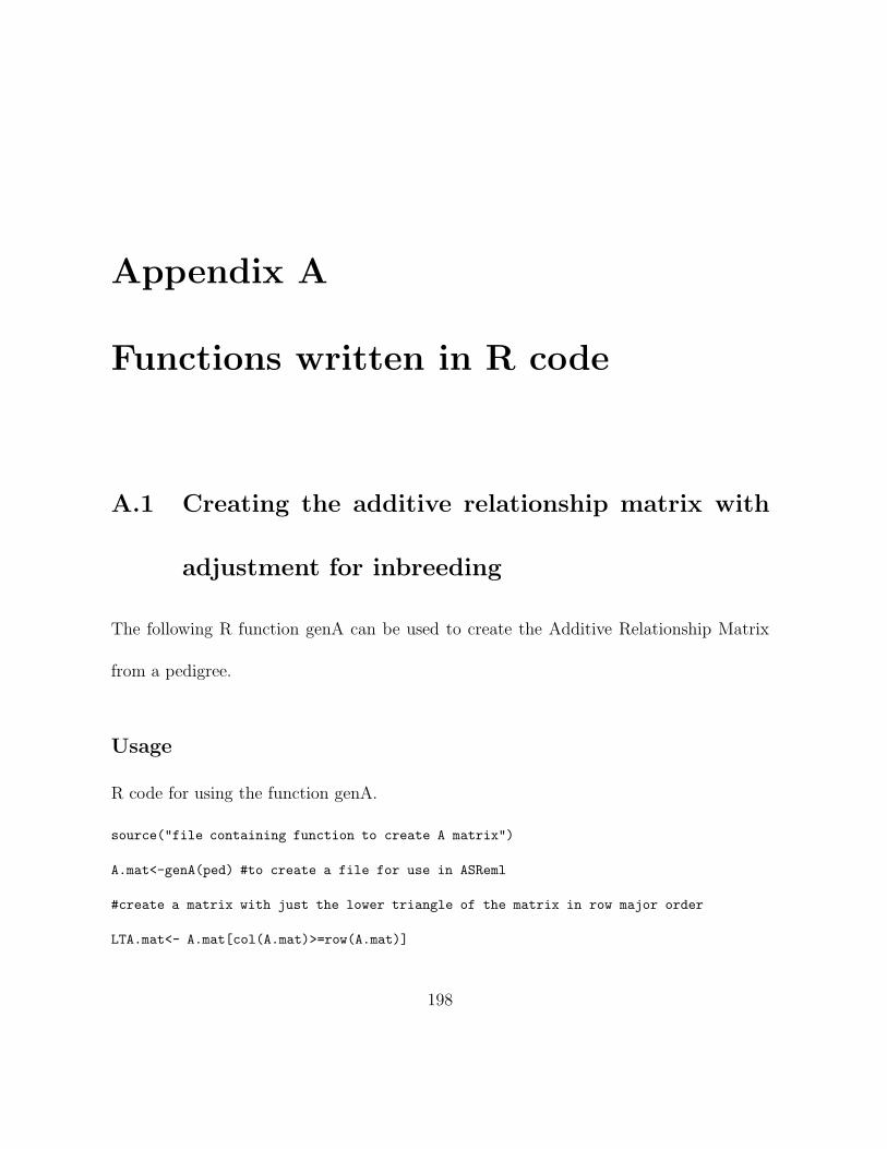
Appendix A
Functions written in R code
A.1 Creating the additive relationship matrix with
adjustment for inbreeding
The following R function genA can be used to create the Additive Relationship Matrix
from a pedigree.
Usage
R code for using the function genA.
source("file containing function to create A matrix")
A.mat<-genA(ped) #to create a file for use in ASReml
#create a matrix with just the lower triangle of the matrix in row major order
LTA.mat<- A.mat[col(A.mat)>=row(A.mat)]
198

Appendix A
#create row and column attributes for ASReml
#wheret m x m is the dimensions of the A.mat
row<-rep(1:m,1:m) #creates a vector 1 2 2 3 3 3 4 4 4 4 5 5 5 5 5 etc
#function to generate columns
source("file containing function to create columns")
column<-funho(m)
#creates a vector 1 1 2 1 2 3 1 2 3 4 1 2 3 4 5 etc
#create a data frame
A.ls<-cbind(row,column,LTA.mat)
dim(A.ls)
Anew.ls<-matrix(NA,ncol=3,nrow=dim(A.ls)[1])
k<-1
for(i in1:dim(A.ls)[1])
{if(A.ls[i,3]>0)
{Anew.ls[k,]<-A.ls[i,] cat("iteration ", i,"\n" ) k<-k+1} }
# trim list down to appropriate size as not all elements of A will be non-zero
is.na(Anew.ls[100:101,3])
Anew.ls<-Anew.ls[1:108831,]
# create a tab delimited txt file for ASReml (sep default is comma separated)
write.table(Anew.ls,file="A.grm",sep="\t",row.names=F)
Arguments
ped this is a pedigree data file with four columns: individual (1 to n), parent1, parent2,
generation. The pedigree should be ordered such that parents proceed their progeny.
199

Appendix A
If the parents of an individual are unknown then set value of parent1/parent2=0.
If the individual is a base parent or represents ”F1” or ”straight cross” between
parents enter 1 in generation column. Otherwise, enter the appropriate generation
eg. F3 (selfed) would be a single seed descent from an F1 with generation=3. If the
individual is a Double Haploid line enter generation=999.
R code for function genA
genA<-function(data) #final
{
ped <- data #read in pedigree data
n<-max(ped[,1])
t<-min(ped[,1]) #set to minimum number of individuals
A<-matrix(0,nrow=n,ncol=n)
#start loop
while(t <=n)
{#while loop
s<-max(ped[t,2],ped[t,3])
d<-min(ped[t,2],ped[t,3])
#both parents are known (including DH and inbreeding ie. other than F1 generation)
if (s>0 & d>0 ) #look at row for individual t and the column parent1 and parent 2
{#if both
if (ped[t,4]==999 & s!=d) #DH without both parents the same
200

Appendix A
{ warning("both parents of DH should be the same, parents different
for at least one DH individual")
NULL }
#diag element A[valueparent 1 of t and parent 2 of t]
A[t,t]<- 2-0.5^(ped[t,4]-1)+0.5^(ped[t,4])*A[ped[t,2],ped[t,3]]
for(j in 1:(t-1))#as do it progressively only want j < t
{ #for loop
A[t,j]<- 0.5*(A[j,ped[t,2]]+A[j,ped[t,3]])
A[j,t]<- A[t,j]
} #for loop
}#if both
#one parent is known (including DH and inbreeding ie. other than F1 generation)
if (s>0 & d==0 )
{#if one
if ( ped[t,4]==999) #DH with one parent recorded and other zero
{ warning("both parents of DH should be the same,
one parent equal to zero for at least one DH individual")
NULL }
A[t,t]<- 2-0.5^(ped[t,4]-1)
for(j in 1:(t-1))#as do it progressively only want j < t
{ #for loop
A[t,j]<-0.5*A[j,s]
A[j,t]<-A[t,j]
201

Appendix A
} #for loop
} #if one
#no parents are known (including DH and inbreeding ie. other than F1 generation)
if (s==0 )
{
A[t,t]<- 2-0.5^(ped[t,4]-1)
}
#SHOW ITERATIONS IN R OUPUT
cat(" iteration ", t ,"\n")
#update number of iterations
t<-t+1
} #while loop
A
}
R code for function funho
funho<-function(n)
{
i <- 2 #set the number of iterations to two
maxit<-n #set the maxit to n
newt<-1 #set initial value of newt to 1
#start loop
while( i <=maxit)
202

Appendix A
{#while
t<-1:i
newt<-c(newt,t)
#update number of iterations
i<-i+1
#SHOW ITERATIONS IN Splus OUPUT
cat(" iteration ", i )
}#while
newt
}
A.2 Simulation code to generate data models
Initial values for the data models are created as follows using R code
#work out what the epistatic proportion of the total genetic variance should be
propi<-c(0.25,0.5,0.75)
#proportion of variance that due to additive (divide by 2 since g=a*2+i)
propa<-(1-propi)/2
203

Appendix A
gvar05<-0.5
#now create gvar epistatic
ivar05<-propi*gvar05
#now create gvar additive
avar05<-propa*gvar05
sitemn05<-10
The following function fieldgenA is used as follows to creates the simulated data models.
The example shows the data model with genetic variance of 0.5 and additive genetic
variance of 25%.
datam200gv05ap25<-list() #instead of field run
for(i in 1:500)
{datam200gv05ap25[[i]]<-fieldgenA(fdes,sitemn05,1,ivar05[3],avar05[3],A200.mat)
}
fieldgenA <- function(genodes,sitemn,evar,ivar,avar,A.mat)#,des=NULL)
{
# code to generate simulated data for a single trial
# genodes a dataframe containing trial design
# with variables Site,Column,Row,Replicate,Trt
# sitemn site mean
# evar error variance
# ivar epistatic variance
# avar additive variance
204
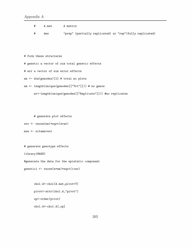
Appendix A
# A.mat A matrix
# des "prep" (partially replicated) or "rep"(fully replicated)
# form these structures
# genetic a vector of sim total genetic effects
# err a vector of sim error effects
nn <- dim(genodes)[1] # total no plots
nm <- length(unique(genodes[["Trt"]])) # no genos
nr<-length(unique(genodes[["Replicate"]])) #no replicates
# generate plot effects
err <- rnorm(nn)*sqrt(evar)
mue <- sitemn+err
# generate genotype effects
library(MASS)
#generate the data for the epistatic component
genetici <- rnorm(n=nm)*sqrt(ivar)
chol.A<-chol(A.mat,pivot=T)
pivot<-attr(chol.A,"pivot")
op<-order(pivot)
chol.A<-chol.A[,op]
205
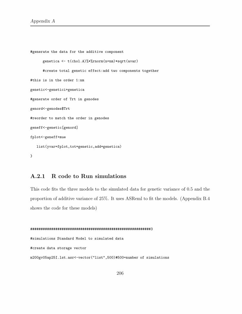
Appendix A
#generate the data for the additive component
genetica <- t(chol.A)%*%rnorm(n=nm)*sqrt(avar)
#create total genetic effect:add two components together
#this is in the order 1:nm
genetic<-genetici+genetica
#generate order of Trt in genodes
genord<-genodes$Trt
#reorder to match the order in genodes
geneff<-genetic[genord]
fplot<-geneff+mue
list(yvar=fplot,tot=genetic,add=genetica)
}
A.2.1 R code to Run simulations
This code fits the three models to the simulated data for genetic variance of 0.5 and the
proportion of additive variance of 25%. It uses ASReml to fit the models. (Appendix B.4
shows the code for these models)
##########################################################3
#simulations Standard Model to simulated data
#create data storage vector
m200gv05ap25I.lst.asr<-vector("list",500)#500=number of simulations
206
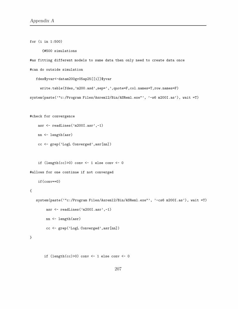
Appendix A
for (i in 1:500)
{#500 simulations
#as fitting different models to same data then only need to create data once
#can do outside simulation
fdes$yvar<-datam200gv05ap25[[i]]$yvar
write.table(fdes,’m200.asd’,sep=’,’,quote=F,col.names=T,row.names=F)
system(paste(’"c:/Program Files/Asreml2/Bin/ASReml.exe"’, ’-s6 m200I.as’), wait =T)
#check for convergence
asr <- readLines(’m200I.asr’,-1)
nn <- length(asr)
cc <- grep(’LogL Converged’,asr[nn])
if (length(cc)>0) conv <- 1 else conv <- 0
#allows for one continue if not converged
if(conv==0)
{
system(paste(’"c:/Program Files/Asreml2/Bin/ASReml.exe"’, ’-cs6 m200I.as’), wait =T)
asr <- readLines(’m200I.asr’,-1)
nn <- length(asr)
cc <- grep(’LogL Converged’,asr[nn])
}
if (length(cc)>0) conv <- 1 else conv <- 0
207

Appendix A
msep <- msepat<- selOK <- selOKat<- NA
resvar<- gam <- logl<-NA
mtr<- mtra <- mpsel<-mpasel<- NA
if (conv==1) {#if
#if job converged get variety by site predictions
#if a one-stage job then skip 8 lines on .pvs file
pvs<-readLines(’m200I.pvs’,-1)
pp<-grep(’Standard_Error’,pvs)
writeLines(pvs[(pp+1):(ng+pp)],’m200I.prd’)
pvs <- read.table(’m200I.prd’)
names(pvs) <- c(’variety’,’pred’,’se’,’dum’)
pvs$true <- as.vector(datam200gv05ap25[[i]]$tot)
pvs$atrue<-as.vector(datam200gv05ap25[[i]]$add)
msep.full <- as.vector((pvs$pred-pvs$true)^2)
msepat.full <- as.vector((pvs$pred-pvs$atrue)^2)
#calculate average msep for each site
msep <- mean(msep.full)
msepat <- mean(msepat.full)
#calculate number of varieties in common between true and predicted
#when selecting top 25
ge.pred <-matrix(pvs$pred,ncol=1)
ge.true <- matrix(pvs$true,ncol=1)
ge.atrue <- matrix(pvs$atrue,ncol=1)#additive actual values
dimnames(ge.pred)<- dimnames(ge.true) <-dimnames(ge.atrue)<- list(1:ng,"eff")
208

Appendix A
#now get the top 20 genotype numbers
top25.true<-names(ge.true[order(rank(-ge.true)),1])[1:25]
# top25.true <- names(ge.true[rev(order(ge.true[,1])),1])[1:25]#alternative
top25.pred <- names(ge.pred[order(rank(-ge.pred)),1])[1:25]
top25.atrue<-names(ge.atrue[order(rank(-ge.atrue)),1])[1:25]
#number of lines the same in true vs predicted
selOK <- length(top25.true[is.element(top25.true,top25.pred)])#
selOKat <- length(top25.atrue[is.element(top25.atrue,top25.pred)])
#mean of population true values and mean of selected true values
mtr<-mean(ge.true)
mtra<-mean(ge.atrue)
mpsel<-mean(ge.true[as.numeric(top25.pred)])
mpasel<-mean(ge.atrue[as.numeric(top25.pred)])
}#if
# save residual variance and GxE variance parameters
#save line number xx for start of variance parameters
for (j in 1:nn)
{
ss <- grep(’Source’,asr[j])
if (length(ss)>0) xx <- j
}
#residual variance
for (j in (xx+2))
{
209

Appendix A
resvar <- as.numeric(substring(asr[j],51,64))
}
#treatment variance
for (j in (xx+1) ) #7*3-1fa2
{
gam <- as.numeric(substring(asr[j],51,64))
}
# also save logl
for (j in (xx-3))
{
logl <- as.numeric(substring(asr[j],12,18))
}
m200gv05ap25I.lst.asr[[i]]<-list(conv=conv,msep=msep,msepat=msepat,selOK=selOK,
selOKat=selOKat,gam=gam,resvar=resvar,logl=logl,
mtr=mtr,mtra=mtra,mpsel=mpsel,mpasel=mpasel)
}#for
##########################################################3
##########################################################3
#Fit Additive model to simulated data
210

Appendix A
#create data storage vector
m200gv05ap25A.lst.asr<-vector("list",500)#500=number of simulations
for (i in 1:500)
{#500 simulations
#as fitting different models to same data then only need to create data once
#can do outside simulation
fdes$yvar<-datam200gv05ap25[[i]]$yvar
write.table(fdes,’m200.asd’,sep=’,’,quote=F,col.names=T,row.names=F)
system(paste(’"c:/Program Files/Asreml2/Bin/ASReml.exe"’, ’-s6 m200A.as’), wait =T)
#check for convergence
asr <- readLines(’m200A.asr’,-1)
nn <- length(asr)
cc <- grep(’LogL Converged’,asr[nn])
if (length(cc)>0) conv <- 1 else conv <- 0
#allows for one continue if not converged
if(conv==0)
{
system(paste(’"c:/Program Files/Asreml2/Bin/ASReml.exe"’, ’-cs6 m200A.as’), wait =T)
asr <- readLines(’m200A.asr’,-1)
nn <- length(asr)
cc <- grep(’LogL Converged’,asr[nn])
211
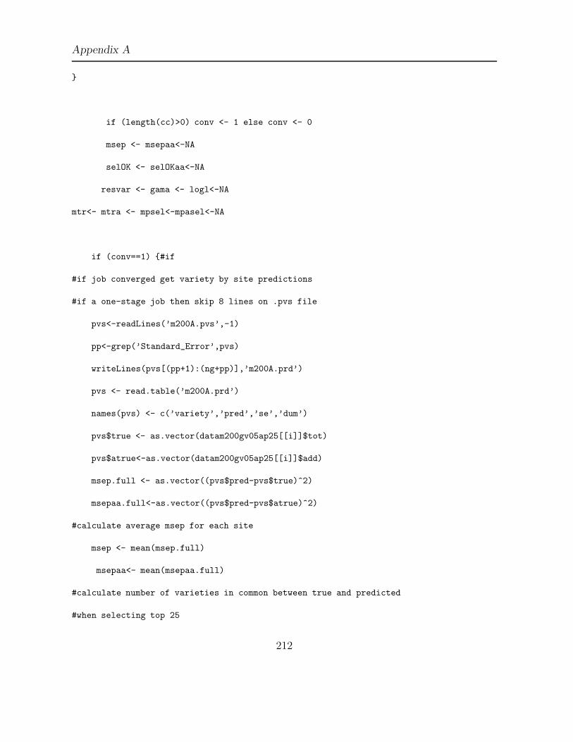
Appendix A
}
if (length(cc)>0) conv <- 1 else conv <- 0
msep <- msepaa<-NA
selOK <- selOKaa<-NA
resvar <- gama <- logl<-NA
mtr<- mtra <- mpsel<-mpasel<-NA
if (conv==1) {#if
#if job converged get variety by site predictions
#if a one-stage job then skip 8 lines on .pvs file
pvs<-readLines(’m200A.pvs’,-1)
pp<-grep(’Standard_Error’,pvs)
writeLines(pvs[(pp+1):(ng+pp)],’m200A.prd’)
pvs <- read.table(’m200A.prd’)
names(pvs) <- c(’variety’,’pred’,’se’,’dum’)
pvs$true <- as.vector(datam200gv05ap25[[i]]$tot)
pvs$atrue<-as.vector(datam200gv05ap25[[i]]$add)
msep.full <- as.vector((pvs$pred-pvs$true)^2)
msepaa.full<-as.vector((pvs$pred-pvs$atrue)^2)
#calculate average msep for each site
msep <- mean(msep.full)
msepaa<- mean(msepaa.full)
#calculate number of varieties in common between true and predicted
#when selecting top 25
212

Appendix A
ge.pred <-matrix(pvs$pred,ncol=1)#total predicted values
ge.true <- matrix(pvs$true,ncol=1)#total actual values
ge.atrue <- matrix(pvs$atrue,ncol=1)#additive actual values
dimnames(ge.pred)<- dimnames(ge.true) <- dimnames(ge.atrue)
<-list(1:ng,"eff")
#now get the top 20 genotype numbers
top25.true<-names(ge.true[order(rank(-ge.true)),1])[1:25]
top25.atrue<-names(ge.atrue[order(rank(-ge.atrue)),1])[1:25]
# top25.true <- names(ge.true[rev(order(ge.true[,1])),1])[1:25]#alternative
top25.pred <- names(ge.pred[order(rank(-ge.pred)),1])[1:25]
#number of lines the same in true vs predicted
selOK <- length(top25.true[is.element(top25.true,top25.pred)])
selOKaa <- length(top25.atrue[is.element(top25.atrue,top25.pred)])
#mean of population true values and mean of selected true values
mtr<-mean(ge.true)
mtra<-mean(ge.atrue)
mpsel<-mean(ge.true[as.numeric(top25.pred)])
mpasel<-mean(ge.atrue[as.numeric(top25.pred)])
}#if
# save residual variance and GxE variance parameters
#save line number xx for start of variance parameters
for (j in 1:nn)
{
213

Appendix A
ss <- grep(’Source’,asr[j])
if (length(ss)>0) xx <- j
}
#residual variance
for (j in (xx+1))
{
resvar <- as.numeric(substring(asr[j],51,64))
}
#addit treatment variance
for (j in (xx+2) ) #7*3-1fa2
{
gama <- as.numeric(substring(asr[j],51,64))
}
# also save logl
for (j in (xx-3))
{
logl <- as.numeric(substring(asr[j],12,18))
}
m200gv05ap25A.lst.asr[[i]]<-list(conv=conv,msep=msep,msepaa=msepaa,
selOK=selOK,selOKaa=selOKaa,gama=gama,resvar=resvar,logl=logl,
mtr=mtr,mtra=mtra,mpsel=mpsel,mpasel=mpasel)
214

Appendix A
}#for
##########################################################3
#Fit Extended data to simulated data
#create data storage vector
m200gv05ap25AI.lst.asr<-vector("list",500)#500=number of simulations
for (i in 1:500)
#i<-47
{#200 simulations
#as fitting different models to same data then only need to create data once
#can do outside simulation
fdes$yvar<-datam200gv05ap25[[i]]$yvar
write.table(fdes,’m200.asd’,sep=’,’,quote=F,col.names=T,row.names=F)
system(paste(’"c:/Program Files/Asreml2/Bin/ASReml.exe"’, ’-s6 m200AI.as’), wait =T)
#check for convergence
asr <- readLines(’m200AI.asr’,-1)
nn <- length(asr)
cc <- grep(’LogL Converged’,asr[nn])
215

Appendix A
if (length(cc)>0) conv <- 1 else conv <- 0
#allows for one continue if not converged
if(conv==0)
{
system(paste(’"c:/Program Files/Asreml2/Bin/ASReml.exe"’, ’-cs6 m200AI.as’), wait =T)
asr <- readLines(’m200AI.asr’,-1)
nn <- length(asr)
cc <- grep(’LogL Converged’,asr[nn])
}
if (length(cc)>0) conv <- 1 else conv <- 0
msep <-msepat<-msepaa<-NA
selOK <- selOKaa<-selOKat<-NA
resvar <- NA
gama<-gami <- logl<-NA
mtr<- mtra <- mpsel<-mpasel<-mpatsel<- NA
if (conv==1) {#if
#if job converged get variety by site predictions
#if a one-stage job then skip 8 lines on .pvs file
pvs<-readLines(’m200AI.pvs’,-1) #predictions
pp<-grep(’Standard_Error’,pvs)
writeLines(pvs[(pp[1]+1):(ng+pp[1])],’m200AI1.prd’)#total predictions
writeLines(pvs[(pp[2]+1):(ng+pp[2])],’m200AI2.prd’)#additive predictions
216

Appendix A
tmp<-read.table(’m200AI2.prd’)
names(tmp) <- c(’variety’,’apred’,’se’,’dum’)
pvs <- read.table(’m200AI1.prd’)
names(pvs) <- c(’variety’,’pred’,’se’,’dum’)
pvs$true <- as.vector(datam200gv05ap25[[i]]$tot) #true total values
pvs$atrue<-as.vector(datam200gv05ap25[[i]]$add) #true additive values
pvs$apred<-tmp$apred
msep.full <- as.vector((pvs$pred-pvs$true)^2)
msepat.full<-as.vector((pvs$pred-pvs$atrue)^2)
msepaa.full<-as.vector((pvs$apred-pvs$atrue)^2)
#calculate average msep for each site
msep <- mean(msep.full)
msepat <- mean(msepat.full)
msepaa <- mean(msepaa.full)
#calculate number of varieties in common between true and predicted
#when selecting top 25
ge.apred <-matrix(pvs$apred,ncol=1)
ge.pred <-matrix(pvs$pred,ncol=1)
ge.true <- matrix(pvs$true,ncol=1)
ge.atrue <- matrix(pvs$atrue,ncol=1)
dimnames(ge.pred)<- dimnames(ge.apred)<- dimnames(ge.true)
<- dimnames(ge.atrue) <-list(1:ng,"eff")
#now get the top 20 genotype numbers
217

Appendix A
top25.true<-names(ge.true[order(rank(-ge.true)),1])[1:25]
top25.atrue<-names(ge.atrue[order(rank(-ge.atrue)),1])[1:25]
# top25.true <- names(ge.true[rev(order(ge.true[,1])),1])[1:25]#alternative
top25.pred <- names(ge.pred[order(rank(-ge.pred)),1])[1:25]
top25.apred <- names(ge.apred[order(rank(-ge.apred)),1])[1:25]
#number of lines the same in true vs predicted
selOK <- length(top25.true[is.element(top25.true,top25.pred)])
selOKat <- length(top25.atrue[is.element(top25.atrue,top25.pred)])
selOKaa <- length(top25.atrue[is.element(top25.atrue,top25.apred)])
#mean of population true values and mean of selected true values
mtr<-mean(ge.true)
mtra<-mean(ge.atrue)
mpsel<-mean(ge.true[as.numeric(top25.pred)])
mpasel<-mean(ge.atrue[as.numeric(top25.apred)])
mpatsel<-mean(ge.atrue[as.numeric(top25.pred)])
}#if
# save residual variance and GxE variance parameters
#save line number xx for start of variance parameters
for (j in 1:nn)
{
ss <- grep(’Source’,asr[j])
218

Appendix A
if (length(ss)>0) xx <- j
}
#residual variance
for (j in (xx+2))
{
resvar <- as.numeric(substring(asr[j],51,64))
}
#addit treatment variance
for (j in (xx+3) ) #7*3-1fa2
{
gama <- as.numeric(substring(asr[j],51,64))
}
#epistatic treatment variance
for (j in (xx+1) ) #7*3-1fa2
{
gami <- as.numeric(substring(asr[j],51,64))
}
# also save logl
for (j in (xx-5))
{
219
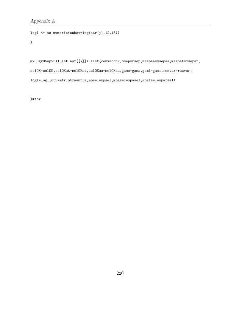
Appendix A
logl <- as.numeric(substring(asr[j],12,18))
}
m200gv05ap25AI.lst.asr[[i]]<-list(conv=conv,msep=msep,msepaa=msepaa,msepat=msepat,
selOK=selOK,selOKat=selOKat,selOKaa=selOKaa,gama=gama,gami=gami,resvar=resvar,
logl=logl,mtr=mtr,mtra=mtra,mpsel=mpsel,mpasel=mpasel,mpatsel=mpatsel)
}#for
220
Appendix B
ASReml code
B.1 ASReml code for fitting the Extended model in
the wheat example (single site)
The A matrix (created in ICIS) is supplied to ASReml as a .grm file which defines the
lower triangle of the A matrix or as a .giv file which defines the lower triangle of the
inverse of the A matrix. There are two equivalent ways to approach the fitting of the
models discussed in Section 4.2.1, the difference depends on whether the A matrix or
it’s inverse include only lines with pedigree information or whether they are extended to
include all the lines of interest. Note: although the A matrix includes all lines of interest
in the latter approach, the genetic components for the lines with and without pedigree
information are still fitted as separate terms.
221

Appendix B
In the first approach the A matrix or inverse are created based only on elite lines
with pedigree information. The two random terms gt and ht for lines with and without
pedigree information are represented in ASReml code by two factors denoted by known
and unknown respectively. The factor known, has levels corresponding to the 129 lines
with pedigree information and has missing values for the lines without pedigree informa-
tion. The factor unknown, has levels corresponding to the 123 lines without pedigree
information and has missing values for the lines with pedigree.
In the second approach an A matrix or inverse is created that includes all lines of
interest by extending the A matrix to include lines without pedigree. Each of the lines
without pedigree information is included with a diagonal term of 2, (as all elite lines
are assumed to be completely homozygous lines). The off-diagonal terms (with all other
lines) are assumed to be zero. Thus lines without pedigree information are assumed to
be completely unrelated to other lines. Off-diagonal terms of zero are not included in the
.grm or .giv file as any excluded terms in these files are assumed zero.
A factor with name ped is created with levels 1, 2 and 3 corresponding to lines with
and without pedigree and the filler line respectively. A single factor line is required
with 252 levels corresponding to the 252 elite lines, NA is used for the filler line. The
at(ped, level).line ASReml qualifier is used to fit the two random terms gt and ht for lines
with and without pedigree information. The ASReml code is given in Appendix B.1.
So that in fact although specified in the A matrix, the lines without pedigree infor-
222

Appendix B
mation are not associated with the A matrix owing to the exclusion of a G-structure for
at(ped,2).line.
For the reasons below the first approach is recommended as the approach of choice:
1. the A matrix does not need to be expanded to include lines without pedigree
2. Approach 1 is easier to expand when fitting the MET analysis
3. At Robinvale there were convergence problems when fitting Approach 2
In summary Approach 1 was found to be easier to use and more stable computationally.
ASReml code for Approach 1
single trial model
block 2 #block term -factor with 2 levels
column 12 #column term -factor with 12 levels
row 42 #row term -factor with 42 levels
yield #response variable
lrow #linear row term -variable centred at mean row
lcol #linear column term -variable centred at mean column
line 253 #factor with 253 levels
ped 3 #factor with three levels: 1=lines with pedigree,
#2=lines without pedigrees, 3=filler line
known 129 #factor with levels 1:129, for lines with pedigrees
#and "NA"s for lines without pedigree & filler lines
unknownped 123 #factor with levels 1:123 for lines without pedigree
223

Appendix B
#and "NA"s for lines with pedigrees & filler line
stage3.giv #the A inverse file
stage3.asd !skip1 !mvinclude!slow !maxit 20 #the data file for a single trial
yield ~ mu ped, #the fixed terms of the model
!r unknownped, #random term for lines without pedigree
known ide(known), #additive and epistatic random terms
#for lines with pedigree
block units #other random terms of the model
!f mv #estimate missing values
1 2 1 #number of sites, number of R-structure components,
#number of G- structures
12 column AR1 #number of columns with AR1 structure
42 row AR1 #number of rows with AR1 structure
known 1 #G structure for lines with pedigree
known 0 GIV1 !GP #specifies the file stage3.giv
#as the corresponding G-structure
ASReml code for Approach 2
single trial model
block 2 #block term -factor with 2 levels
column 12 #column term -factor with 12 levels
row 42 #row term -factor with 42 levels
yield #response variable
lrow #linear row term -variable centred at mean row
224

Appendix B
lcol #linear column term -variable centred at mean column
line 253 #factor with 253 levels
ped 3 #factor with three levels: 1=lines with pedigree,
#2=lines without pedigrees, 3=filler line
known 129 #factor with levels 1:129, for lines with pedigrees
#and "NA"s for lines without pedigree & filler line
unknown 123 #factor with levels 1:123 for lines without pedigree
#and "NA"s for lines with pedigrees & filler line
stage3.giv #the A inverse file
stage3.asd !skip1 !mvinclude!slow !maxit 20 #the data file for a single trial
yield ~ mu ped, #the fixed terms of the model
!r at(ped,2).line, #random term for lines without pedigree
at(ped,1).line at(ped,1).ide(line), #additive and epistatic random terms
#for lines with pedigree
block units #other random terms of the model
!f mv #estimate missing values
1 2 1 #number of sites, number of R-structure components,
#number of G- structures
12 column AR1 #number of columns with AR1 structure
42 row AR1 #number of rows with AR1 structure
at(ped,1).line 1 #G structure for lines with pedigree
line 0 GIV1 !GP #specifies the file stage3.giv
#as the corresponding G-structure
225

Appendix B
B.2 ASReml code for the final MET Extended model
in the wheat example
The ASReml code for Model 8, Table 4.6, on page 133is shown below. Note: the trial
numbering/ordering in the data set and therefore code below is not consistent with that
presented in Chapter 4, where trials are presented and ordered alphabetically.
Met on 14 trials: #with terms from single trial models included
block 2
column 18
row 42
yield
horder 2
plotsize
trial 14
lrow
lcol
line 253 #factor with 253 levels
ped 3 #factor with three levels: 1=lines with pedigree,
#2=lines without pedigrees, 3=filler line
known 129 #factor with levels 1:129, for lines with pedigrees
#and "NA"s for lines without pedigree & filler line
unknown 123 #factor with levels 1:123 for lines without pedigree
#and "NA"s for lines with pedigrees & filler line
226

Appendix B
itrial 8 !A #factor with 8 levels corresponding to trials
#with epistatic components
stage3.giv !GIV #the A inverse file
st3all.txt !skip 1 !mvinclude !MAXIT 30 !SLOW #the data file for all trials
yield~ -1 trial.ped,
at(trial,2).lcol, #Kapunda
at(trial,3).lcol, #Mingenew
at(trial,6).row, #Wongan Hills
at(trial,7).lrow , #Scaddon
at(trial,8).lrow , #Temora
at(trial,10).lcol, #Pinnaroo
at(trial,10).lrow,
at(trial,10).plotsize,
at(trial,11).lrow, #Coomalbidgup
at(trial,11).row:lcol,
at(trial,11).horder,
at(trial,12).lcol, #Narrandera
at(trial,14).lrow, #minnipa
!r trial.block,
xfa(trial,1).unknown, #line without pedigree
xfa(trial,2).giv(known,1) xfa(itrial,1).ide(known), #lines with pedigree
at(trial,1).column 84000, #Coonalpyn
at(trial,4).column 964, #Merredin
at(trial,6).row 349, #Wongan Hills
at(trial,7).column 56000, #Scaddon
227

Appendix B
at(trial,8).column 24450, #Temora
at(trial,9).column 166000, #Narrabri
at(trial,9).row 24000,
at(trial,10).column 9600, #Pinnaroo
at(trial,10).spl(column) 15000,
at(trial,11).column 38300, #Coomalbidgup
at(trial,11).spl(row) 19500,
at(trial,13).row 316, #Robinvale
at(trial,14).spl(row) 333, #Minnipa,
-at(trial,1).units 22000 ,
-at(trial,2).units 52000 ,
-at(trial,3).units 17700 ,
-at(trial,4).units 3400,
-at(trial,5).units 20300 ,
-at(trial,6).units 3200 ,
-at(trial,7).units 32700,
-at(trial,8).units 20490 ,
-at(trial,9).units 91000 ,
-at(trial,10).units 26100 ,
-at(trial,11).units 53100 ,
-at(trial,12).units 6100,
-at(trial,14).units 2200,
!f mv
14 2 4 !NODISPLAY # number of trials # number of R-str # G-str
12 column ID !S2=84000 #trial 1 Coonalpyn
228

Appendix B
42 row AR1 0.63
12 column AR1 0.21 !S2=274000 #trial 2 Kapunda
42 row AR1 0.69
12 column ID !S2=65000 #trial 3 Mingenew
42 row AR1 0.62
12 column ID !S2=7400 #trial 4 Merredin
42 row AR1 0.50
12 column AR1 0.32 !S2=167000 #trial 5 Roseworthy
42 row AR1 0.83
12 column AR1 0.20 !S2=6700 #trial 6 Wongan Hills
42 row AR1 0.50
12 column ID !S2=60000 #trial 7 Scaddon
42 row AR1 0.40
12 column ID !S2=82000 #trial 8 Temora
42 row AR1 0.62
18 column AR1 0.13 !S2=1068000 #trial 9 Narrabri
28 row AR1 0.33
12 column AR1 0.31 !S2=66000 #trial 10 Pinnaroo
42 row AR1 0.50
12 column ID !S2=75300 #trial 11 Coomalbidgup
42 row AR1 0.24
12 column AR1 0.15 !S2=22100 #trial 12 Narrandera
42 row AR1 0.67
12 column AR1 0.17 !S2=14900 #trial 13 Robinvale
42 row AR1 0.71
229
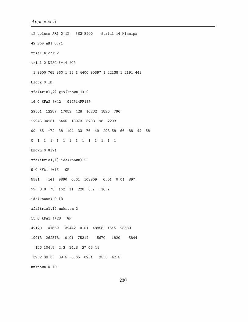
Appendix B
12 column AR1 0.12 !S2=8900 #trial 14 Minnipa
42 row AR1 0.71
trial.block 2
trial 0 DIAG !+14 !GP
1 9500 765 360 1 15 1 4400 90397 1 22138 1 2191 443
block 0 ID
xfa(trial,2).giv(known,1) 2
16 0 XFA2 !+42 !G14P14PF13P
29301 12287 17052 428 16232 1826 796
12945 94251 6465 18973 5203 98 2293
90 65 -72 38 104 33 76 49 293 58 66 88 44 58
0 1 1 1 1 1 1 1 1 1 1 1 1 1
known 0 GIV1
xfa(itrial,1).ide(known) 2
9 0 XFA1 !+16 !GP
5581 141 9890 0.01 103909. 0.01 0.01 897
99 -8.8 75 162 11 228 3.7 -16.7
ide(known) 0 ID
xfa(trial,1).unknown 2
15 0 XFA1 !+28 !GP
42120 41659 32442 0.01 48858 1515 28689
19913 262578. 0.01 75314 5670 1820 5844
126 104.8 2.3 34.8 27 43 44
39.2 38.3 89.5 -3.65 62.1 35.3 42.5
unknown 0 ID
230

Appendix B
B.3 ASReml code for the final MET Extended model
in the sugarcane example
The ASReml code for Model 11, Table 5.3 is shown below. The data.ped is a file containing
the pedigree file, from which ASReml calculates the inverse of the relationship matrix A−1.
ASReml requires a file which has three columns: clone parent1 parent2. The file must be
ordered with founding individuals first. DB.grm and DW.grm are the dominance between
family and dominance within family line matrices respectively. DW.grm is a scale identity.
The .grm indicates that these are not inverse matrices (ie. DB.grm is Db not D−1b ) and
ASReml will invert them. (A .giv ending would indicate that these were inverse matrices).
ASReml requires just the lower triangle of this matrices. It is important to ensure that
the numbering of lines in the corresponding factors familyB and familyW corresponds
directly to the ordering of rows and columns in the .grm file. Row one and column one of
the Db matrix contain the dominance between relationships of family 1, and this should
correspondingly be labeled as 1 in the familyB factor, similarly for the familyW.
The data.asd is a text file containing the data.
The additive genetic effect with a factor analytic structure of order two for Ga is fitted
by including the term xfa(Site,2).Clone in the random part of the model specification.
231

Appendix B
A factor analytic structure of order one for Gd at 4 sites is fitted by including the term
xfa(dSite,1).giv(familyB,1) and xfa(dSite,1).giv(familyW,2), dSite has 4 levels instead of
6 (the other sites are set to ‘NA’) and so ensures that a dominance effect is just fitted
at these sites and the .giv(,) indicates which .grm file to associate with each effect. In
addition, these two dominance genetic effects must be constrained to be equal. This is
achieved most simply by the !=%ABCDEFG command in the G-structure line of both
these terms. The residual non-additive genetic effect has a factor analytic structure of
order one for Gi at 3 sites.
!WORK 500
MET
Subtrial !A
Trial !A
row 58
column 30
block 2
tch
ccs
Clone !P !LL 26
lrow
lcol
fam !A
familyn
familyas 187
232

Appendix B
line 48
famlin 2267 !A !SORT
iTrial 3 !A # Sites BIN1 MQN MYB
dTrial 4 !A # Sites BIN1 BIN2 FMD ISS
CAT99_FAT03SN.ped !skip 1 !ALPHA #pedigree file from which the ainverse is formed
DB.grm !skip 1 !GIV #DOMINANCE MATRIX BETWEEN FAMILY
DW.grm !skip 1 !GIV #DOMINANCE MATRIX WITHIN FAMILY
final.asd !skip 1 !mvinclude !maxit 50 !extra 6 #!AISING
ccs~-1 Trial,
at(Subtrial,4).lcol,
at(Subtrial,4).lrow,
at(Subtrial,5).lrow,
!r Trial.Subtrial xfa(Trial,2).Clone xfa(iTrial,1).ide(Clone),
xfa(dTrial,1).giv(familyas,1) xfa(dTrial,1).giv(famlin,2) ,
at(Subtrial,1).block,
at(Subtrial,4).block,
at(Subtrial,6).block,
at(Subtrial,7).block,
at(Subtrial,1).row,
at(Subtrial,11).row,
at(Subtrial,1).column,
at(Subtrial,3).column,
!f mv
11 2 4 !NODISPLAY # number of sites # number of R-str # G-str
14 column AR 0.59 !S2=2.86 #Subtrial 1
233

Appendix B
8 row AR 0.50
14 column AR 0.168 !S2=1.445 #Subtrial 2
8 row ID
30 column AR 0.07125 !S2=1.36 #Subtrial 3
46 row AR 0.0819
16 column AR 0.439 !S2=0.421 #Subtrial 4
7 row AR 0.246
16 column AR 0.104 !S2=0.474 #Subtrial 5
7 row AR 0.201
14 column ID !S2=0.4205 #Subtrial 6
8 row AR 0.01
14 column AR 0.0814 !S2=0.311 #Subtrial 7
8 row ID
16 column AR 0.29 !S2=0.22 #Subtrial 8
58 row AR 0.25
8 column AR 0.16 !S2=1.04 #Subtrial 9
27 row AR 0.103
16 column AR 0.24 !S2=0.55 #Subtrial 10
7 row ID
16 column AR .02 !S2=0.51 #Subtrial 11
7 row ID
xfa(Trial,2).Clone 2
8 0 XFA2 !+18 !G6P8UZ3U #FOR FA1=2*6
.13 0.001 0.244 0.265 0.824 .001
1.29 0.51 0.50 0.83 0.652 1.19
234

Appendix B
0.1 0.1 0 0.1 0.1 0.1
Clone 0 AINV
xfa(dTrial,1).giv(familyas,1) 2
5 0 XFA1 !+8 !GP !=%ABCDEFGH #FOR FA1=2*4
.7 .001 .2 .001
.87 .84 .04 .72
familyas 0 GIV1
xfa(dTrial,1).giv(famlin,2) 2
5 0 XFA1 !+8 !GP !=%ABCDEFGH #FOR FA1=2*4
.7 .001 .2 .001
.87 .84 .04 .72
famlin 0 GIV2
xfa(iTrial,1).ide(Clone) 2
4 0 XFA1 !+6 !GP #FOR FA1=2*3
0.85 0.54 .1
.4 .4 .4
ide(Clone) 0 ID
235

Appendix B
B.4 ASReml code for fitting the Analysis models
This is example code to fit three analysis models to replicated data. The ASReml code
for the Standard model
2007 simulations for g=i model
Site 1
Column 8
Row 50
Replicate 2
Trt 200
yvar
m200.asd !mvinclude !skip=1 !maxit 35 !SLOW #!maxit=1 #!EM
yvar ~ mu !r Trt !f mv
1 1 0 !NODISPLAY
400 0
predict Trt !only Trt
The ASReml code for the Additive model
2007 simulations for g=a model
Site 1
236

Appendix B
Column 8
Row 50
Replicate 2
Trt 200
yvar
A200.giv !skip 1 !GIV
m200.asd !mvinclude !skip=1 !maxit 35 !SLOW #!maxit=1 #!EM5
yvar ~ mu !r Trt !f mv
1 1 1 !NODISPLAY
400 0
Trt 1
Trt 0 GIV1 0.1 !GP
predict Trt !only Trt
The ASReml code for the Extended model
2007 simulations for g=a +i model
Site 1
Column 8
Row 50
Replicate 2
Trt 200
yvar
237

Appendix B
A200.giv !skip 1 !GIV
m200.asd !mvinclude !skip=1 !maxit 35 !SLOW #!maxit=1 #!EM 5
yvar ~ mu !r Trt ide(Trt) !f mv
1 1 1 !NODISPLAY
400 0
Trt 1
Trt 0 GIV1 0.1 !GP
predict Trt !only Trt ide(Trt)
predict Trt !only Trt
238
Bibliography
Akaike, H. (1974). A new look at statistical model identification. IEEE transactions on
automatic control AU-19, 716–722.
Bernardo, R. (1994). Prediction of maize single-cross performance using rflps and infor-
mation from related hybrids. Crop Science 34, 20–25.
Bernardo, R. (1996). Best linear unbiased prediction of maize single-cross performance.
Crop Science 36, 50–56.
Besag, J. & Kempton, R. (1986). Statistical analysis of field experiments using neigh-
bouring plots. Biometrics 42, 231–251.
Brown, D., Tier, B., Reverter, A., Banks, R., & Graser, H. (2000). OVIS: A multiple trait
breeding value estimation program for genetic evaluation of sheep. Wool Technology
and Sheep Breeding 48.
BSES (1984). The Standard laboratory manual for Australian Sugar Mills, volume 1.
Bureau of Sugar Experiment Stations, Indooroopilly, QLD. Australia, principles and
practices edition.
239

BIBLIOGRAPHY
Cockerham, C. C. (1954). An extension of the concept of partitioning hereditary variance
for analysis of covariances among relatives when epistasis is present. Genetics 39,
859–882.
Cockerham, C. C. (1983). Covariances of relatives from self-fertilization. Crop Science
23, 1177–1180.
Cockerham, C. C. & Weir, B. S. (1984). Covariances of relatives stemming from a popu-
lation undergoing mixed self and random mating. Biometrics 40, 157–164.
Coombes, N. E. (2002). The reactive tabu search for efficient correlated experimental
designs. PhD thesis, Liverpool John Moores University.
Cooper, M., Brennan, P., & Sheppard, J. (1996). A strategy for yield improvement
of wheat which accomodates large genotype by environment interactions. In plant
adaption and crop improvement, Cooper, M. and Hammer, G. L. pages 487–512.
Cooper, M. & Hammer, G. L. (2005). Preface to special issue: Complex traits and
plant breeding-can we understand the complexities of gene-to-phenotype relationships
and use such knowledge to enhance plant breeding outcomes? Australian Journal of
Agricultural Research 56, 869–872.
Cooper, M. & Podlich, D. W. (1999). Genotype x environment interactions, selection
response and heterosis. In Genetics and Exploitation of Heterosis in Crops (ED. J. G.
Coors and S. Pandey) Chapter 8, 81–92.
Costa e Silva, J., Borralho, N. M. G., & Potts, B. M. (2004). Additive and non-additive
240

BIBLIOGRAPHY
genetic parameters from clonally replicated and seedling progenies of Eucalyptus glob-
ulus. Theoretical and Applied Genetics 108, 1113–1119.
Crepieux, S., Lebreton, C., Servin, B., & Charmet, G. (2004). Quantitative trait loci QTL
detection in multicross inbred designs: Recovering QTL identical-by-descent status
information from marker data. Genetics 168, 1737–1749.
Crianiceanu, C. M. & Ruppert, D. (2004). Likelihood ratio tests in linear mixed models
with one variance component. Journal of the Royal Statistical Society:B 66, 165–185.
Crossa, J., Burgueno, J., Cornelius, P. L., McLaren, G., Trethowan, R., & Krishna-
machari, A. (2006). Modelling genotype X environment interaction using additive ge-
netic covariances of relatives for predicting breeding values of wheat genotypes. Crop
Science 46, 1722–1733.
Cullis, B., Gogel, B., Verbyla, A., & Thompson, R. (1998). Spatial analysis of Multi-
Environment early generation trials. Biometrics 54, 1–18.
Cullis, B., Smith, A., & Coombes, N. (2007). On the design of early generation variety
trials with correlated data. Journal of Agricultural, Biological, and Environmental
Statistics 11.
Cullis, B. R. & Gleeson, A. (1991). Spatial analysis of field experiments-an extension to
two dimensions. Biometrics 47, 1449–1460.
Cullis, B. R., Lill, W., Fisher, J., Read, B., & Gleeson, A. (1989). A new procedure for
the analysis of early generation variety trials. Applied Statistics 38, 361–375.
241
BIBLIOGRAPHY
Cullis, B. R., Smith, A. B., & Thompson, R. (2004, Ch 6). Methods and Models in
Statistics in Honour of Professor John Nelder, FRS. Imperial College Press.
Davik, J. & Honne, B. (2005). Genetic variance and breeding values for resistance to
wind-borne disease [Sphaeotheca Macularis (wallr. ex fr.)] in strawberry (Fragaria x
ananassa duch.) estimated by exploring mixed models and spatial models and pedigree
information. Theoretical and Applied Genetics 111, 256–264.
de Boer, I. J. M. & Hoeschele, I. (1993). Genetic evaluation methods for populations with
dominance and inbreeding. Theoretical and Applied Genetics 86, 245–258.
Durel, C. E., Laurens, F., Fouillet, A., & Lespinasse, Y. (1998). Utilization of pedigree
information to estimate genetic parameters from large unbalanced data sets in apple.
Theoretical and Applied Genetics 96, 1077–1085.
Dutkowski, G. W., Costa e Silva, J., Gilmour, A. R., & Lopez, G. A. (2002). Spatial
analysis methods for forest genetic trials. Canadian Journal of Forest Research 32,
2201–2214.
Edwards, J. W. & Lamkey, K. R. (2002). Quantitative genetics of inbreeding in a synthetic
maize population. Crop Science 42, 1094–1104.
Falconer, D. S. & Mackay, T. (1996). Introduction to Quantitative Genetics. Longman
Group Ltd, 4th edition.
Frensham, A., Barr, A. R., Cullis, B. R., & Pelham, S. D. (1998). A mixed model analysis
of 10 years of oat evaluation data: use of agronomic information to explain genotype
242

BIBLIOGRAPHY
by environment interactions. Euphytica 99, 43–56.
Gabriel, K. R. (1971). The biplot graphic display of matrices with application to principal
component analysis. Biometrika 58.
Gilmour, A. R., Cullis, B., & Verbyla, A. P. (1997). Accounting for natural and extraneous
variation in the analysis of field experiments. Journal of Agricultural, Biological, and
Environmental Statistics 2, 269–293.
Gilmour, A. R., Gogel, B., Cullis, B. R., & Thompson, R. (2006). ASReml, user Guide.
Release 2.0. VSN International Ltd., Hemel Hempstead, UK.
Gogel, B. J., Cullis, B. R., & Verbyla, A. P. (1995). REML estimation of multiplicative
effects in multi-environment variety trials. Biometrics 51, 744–749.
Green, P. J., Jennison, C., & Seheult, A. H. (1985). The analysis of field experiments by
least squares smoothing. Journal of the Royal Statistical Society:B 47, 299–315.
Griffing, B. (1956). Concept of general and specific combining ability in relation to diallel
crossing systems. Australian Journal of Biological Science 9, 463–493.
Harris, D. L. (1964). Genotypic covariances between inbred relatives. Genetics 50, 1319–
1348.
Henderson, C. R. (1950). Estimation of genetic parameters (abstract). The Annals of
Mathematical Statistics 21, 309–310.
Henderson, C. R. (1976). A simple method for computing the inverse of a numerator
relationship matrix used in the prediction of breeding values. Biometrics 32, 69–83.
243

BIBLIOGRAPHY
Henderson, C. R. (1984). Applications of Linear Models in Animal Breeding. University
of Guelph: Guelph, Ontario, Canada.
Hoeschele, I. & VanRaden, P. M. (1991). Rapid inversion of dominance relationship
matrices for noninbred populations by including sire by dam subclass effects. Journal
of Dairy Science 74, 557–569.
Holtsmark, G. & Larsen, B. (1905). Om muligheder for at indskraenke de fejl, somved
markforsog betings af jordens uensartethed. Tiddskr. Landbr. Planteavl. 12, 330–351.
Jacquard, A. (1974). The genetic structure of populations. Springer, Berlin Heidelberg
New York.
Jannoo, N., Grivet, L., David, L., & Glaszmann, J.-C. (2004). Differential chromosome
pairing affinities at meiosis in polyploid sugarcane revealed by molecular markers.
Heredity 93, 460–467.
John, J., Ruggiero, K., & Williams, E. (2002). ALPHA(n)-designs. Australian and New
Zealand Journal of Statistics 44, 457–465.
Kelly, A. M., Smith, A. B., Eccleston, J. A., & Cullis, B. R. (2007). The accuracy of
varietal selection using factor analytic models for multi-environment plant breeding
trials. Crop Science 47, 1063–1070.
Kempton, R. A. (1984). The use of biplots in interpreting variety by environment inter-
actions. Journal of Agricultural Science, Cambridge 103, 123–135.
Lo, L. L., Fernando, R. L., Cantet, R. J. C., & Grossman, M. (1995). Theory for mod-
244
BIBLIOGRAPHY
elling means and covariances in a two-breed population with dominance inheritance.
Theoretical and Applied Genetics 90, 49–62.
Lu, P. X., Huber, D. A., & White, T. L. (1999). Potential biases of incomplete linear
models in heritability estimation and breeding value prediction. Canadian Journal of
Forest Research 29, 724–736.
Malecot, G. (1948). Les mathemathiques de l’heredite. Masson, Paris .
Martin, R. J. (1990). The use of time-series models and methods in the analysis of
agricultural field trials. Communications in Statistics 19, 55–81.
Martin, R. J., Eccleston, J. A., & Chan, B. S. P. (2004). Efficient factorial experiments
when the data are spatially correlated. Journal of Statistical Planning and Inference
126, 377–395.
Meuwissen, T. H. E. & Luo, Z. (1992). Computing inbreeding coefficients in large popu-
lations. Genetics Selection Evolution 24, 305–313.
Meyer, K. & Kirkpatrik, M. (2005). Restricted maximum likelihood estimation of genetic
principal components and smoothed covariance matrices. Genetic Selection Evolution
37, 1–30.
Nabugoomu, F., Kempton, R. A., & Talbot, M. (1999). Analysis of a series of trials where
varieties difference in sensitivity to locations. Journal of Agricultural, Biological and
Environmental Statistics 4, 310–325.
Oakey, H., Verbyla, A., Cullis, B., Wei, X., & Pitchford, W. (2007). Joint modelling of
245

BIBLIOGRAPHY
additive and non-additive (genetic line) effects in multi-environment trials. Theoretical
and Applied Genetics 114, 1319–1332.
Oakey, H., Verbyla, A., Pitchford, W., Cullis, B., & Kuchel, H. (2006). Joint modelling
of additive and non-additive genetic line effects in single field trials. Theoretical and
Applied Genetics 113, 809–819.
Panter, D. M. & Allen, F. L. (1995). Using best linear unbiased predictions to enhance
breeding for yield in soybean: I. choosing parents. Crop Science 35, 397–405.
Patterson, H. & Nabugoomu, F. (1992). REML and the analysis of series of crop variety
trials. In Proceedings from the 16th International Biometric Conference pages 77–93.
Patterson, H. D. & Silvey, V. (1980). Statutory and recommended list trials of crop
varieties in the united kingdom. Journal of Royal Statistical Society A 143, 219–252.
Patterson, H. D., Silvey, V., Talbot, M., & Weatherup, S. T. C. (1977). Variability of
yields of cereal varieties in U.K. trials. Journal of Agricultural Science, Cambridge 89,
238–245.
Patterson, H. D. & Thompson, R. (1971). Recovery of inter-block information when block
sizes are unequal. Biometrika 58, 545–554.
Patterson, H. D. & Williams, E. R. (1976). A new class of resolvable incomplete block
designs. Biometrika 63, 83–92.
Piepho, H.-P. (1997). Analyzing genotype-environment data by mixed models with mul-
tiplicative terms. Biometrics 53, 761–767.
246

BIBLIOGRAPHY
Piepho, H.-P., Denis, J. B., & van Eeuwijk, F. A. (1998). Analyzing genotype-environment
data by mixed models with multiplicative terms. Journal of Agricultural, Biological
and Environmental Statistics 3, 161–162.
Podlich, D. W., Cooper, M., & Basford, K. E. (1999). Computer simulation of a selection
strategy to accommoodate genotype-environment interactions in a wheat recurrent
selection programme. Plant Breeding 118, 17–28.
Quaas, R. L. (1976). Computing the diagonal elements and inverse of a large numerator
relationship matrix. Biometrics 32, 949–953.
R Development Core Team (2005). R: A language and environment for statistical comput-
ing. R Foundation for Statistical Computing, Vienna, Austria. ISBN 3-900051-07-0.
Self, S. G. & Liang, K.-Y. (1987). Asymptotic properties of maximum likelihood estima-
tors and likelihood ratio tests under nonstandard conditions. Journal of the American
Statistical Association 82, 605–610.
Smith, A., Cullis, B., & Thompson, R. (2001). Analyzing variety by environmental data
using multiplicative mixed models and adjustments for spatial field trend. Biometrics
57, 1138–1147.
Smith, A. B., Cullis, B. R., & Thompson, R. (2005). The analysis of crop cultivar breeding
and evaluation trials: an overview of current mixed model approaches. Journal of
Agricultural Science 143, 1–14.
Smith, S. P. & Maki-Tanila, A. (1990). Genotypic covariance matrices and their inverses
247

BIBLIOGRAPHY
for models allowing domiance and inbreeding. Genetic Selection Evolution 22, 65–91.
Sneller, C. H. (1994). SAS programs for calculating coefficients of parentage. Crop Science
34, 1679–1680.
Stram, D. O. & Lee, J. W. (1994). Variance components testing in the longitudinal mixed
effects model. Biometrics 50, 1171–1177.
Stuber, C. W. & Cockerham, C. C. (1966). Gene effects and variances in hybrid popula-
tions. Genetics 54, 1279–1286.
Talbot, M. (1984). Yield variability of crop varieties in the U.K. Journal of Agricultural
Science, Cambridge 102, 315–321.
Theobald, C., Talbot, M., & Nabugooomu, F. (2002). A bayesian approach to regional
and local-area prediction from crop variety trials. Journal of agricultural, biological
and environmental statistics 7, 403–419.
Topal, A., Aydin, C., Akgun, N., & Babaoglu, M. (2004). Diallel cross analysis in durum
wheat (Triticum durum Desf.) identification of best parents for some kernel physical
features. Field Crops Research 87, 1–12.
van der Werf, J. H. J. & de Boer, I. J. M. (1989). Influence of non-additive effects on
estimation of genetic parameters in dairy cattle. Journal of Dairy Science 72, 2606–
2614.
van der Werf, J. H. J. & de Boer, I. J. M. (1990). Estimation of additive genetic variances
when base populations are selected. Journal of Animal Science 68, 3124–3132.
248

BIBLIOGRAPHY
Verbyla, A. P., Cullis, B. R., Kenward, M. G., & Welham, S. J. (1999). The analysis of
designed experiments and longitudinal data using smoothing splines (with discussion).
Applied Statistics 48, 269–311.
Verbyla, A. P. & Oakey, H. (2007). The variance-covariance matrix for relatives undergo-
ing mendelian sampling and inbreeding. Unpublished .
Viana, J. M. S. (2005). Dominance, epistasis, heritabilities and expected genetic gain.
Genetics and Molecular Biology 28, 67–74.
Walsh, B. (2005). The struggle to exploit non-additive variation. Australian Journal of
Agricultural Research 56, 873–881.
Whitaker, D., Williams, E. R., & John, J. A. (2006). Cycdesign 3.0: A package for the
computer generation of experimental designs. Hamilton, New Zealand: CycSoftware
Ltd. .
Wilkinson, G. N., Eckert, S. R., Hancock, T. W., & Mayo, O. (1983). Nearest neighbour
(NN) analysis of field experiments. Journal of the Royal Statistical Society:B 45, 151–
211.
Wright, S. (1922). Coefficients of inbreeding and relationship. American Naturalist 56,
330–338.
Zimmerman, D. L. & Harville, D. A. (1991). A random field approach to the analysis of
field plot experiments. Biometrics 47, 223–239.
249