INCOME TAXATION, LABOUR SUPPLY AND SAVING

Income tax conference:Looking forward at 100 Years: Where next for the Income Tax?

27-28 April 2015Tax and Transfer Policy Institute

Crawford School of Public Policy ANU

Patricia AppsUniversity of Sydney Law School , ANU, UTS and IZA

Faculty of Law

Introduction

2015 Tax Discussion Paper: Re:think

“Our tax system needs to support the modern economy.”

Modern economy:Two of the most fundamental changes in the Australian economy since the middle of the 20th century are:

• the decline in fertility, from around 3.5 in 1960’s to 1.9 today• the rise in female labour force participation.

Majority of working age adults live in couple households. Most have two earners. We need a tax system that can take account of this reality and the gender gap in labour supply elasticities.

Faculty of Law

IntroductionRe:think

“While Australia’s tax system has served the nation well over the decades, it is outdated.”“Australia‘s reliance on income taxes remains much the same as it was in the 1950’s…”

Q: Is the Australian income tax structure “much the same” as in 1950?

A: No. The system has changed dramatically.

• Overall progressivity of the rate scale has declined significantly despite rising inequality.

• The individual as the tax unit for families has been replaced by a system of “quasi-joint” taxation, raising MTRs for many partnered mothers as second earners to well above the top MTR of the PIT scale.

Faculty of Law

Overview of presentation

To investigate the effects of these reforms on the economy we present an analysis of the following:

1. Rise in inequality and impact of a less progressive rate scale.

2. Transformation of the 1980s progressive individual-based family income tax into one of “quasi-joint” taxation – female labour supply effects.

3. Impact of high MTRs on 2nd earners on life cycle time use, consumption and household saving.

4. Efficiency merits of a well-designed, individual based, income tax over a consumption tax in a modern economy.

Concluding comment

Faculty of Law

1 Rise in inequality  ABS HES 2003-04 and 2009-10 data for couples: partners aged 20 to 60 and primary earner employed for min. 25 hours/wk.Primary income distribution

Rise in nominal incomes: quintile 1: 28%; quintile 3: 34%; quintile 5: 48%decile 9: 43%; decile 10: 52%; top percentile: 71%

Faculty of Law

025

5075

100

125

150

175

Prim

ary

inco

me,

dol

lars

pa/

1000

1 2 3 4 5

Primary income quintiles

HES03-04 HES09-10

1 Shift in tax burden to “middle”Primary income distribution

Nominal tax cut: quintile 1: $1388; quintile 3: $602; quintile 5: $6421decile 9: $3,907 decile 10: $8,717 (40% of total) top percentile: $48,680.

Faculty of Law

02,

000

4,00

06,

000

8,00

0Ta

x cu

t, do

llars

pa

1 2 3 4 5

Primary income quintiles

1 Shift in tax burden to “middle”

Carefully planned: Accumulated revenue from bracket creep used to fund changes in the rate scale that gave the largest gains to the top.

Shift in tax burden to the “middle” achieved by combining tax cuts at the top with the Low Income Tax Offset.

The LITO raised the zero rated threshold for those on low incomes while simultaneously denying gains for the middle by raising rates further along the distribution, through its withdrawal rate of 4 cents in the dollar. With the GST included, some in the “middle” will have lost.

The LITO has served the sole purpose of reducing the transparency of the true rate scale. The scale is no longer strictly progressive.

Faculty of Law

1 Bracket creep and GST

Re:think and 2015 Intergenerational Report

“…bracket creep affects lower and middle income earners proportionally more than higher income earners.”

Example: average ordinary earnings in 2013-14 around $75,000.

2013-14 ATR 2023-24 ATR INCREMENT37,500 10.3 52,000 17.8 7.575,000 22.7 104,000 27.4 4.7150,000 30.5 208,000 34.3 3.8

Faculty of Law

Check with ABS HES 2009‐10 dataIncomes indexed to 2013-14 and to 2023-24$37,500 mean of 1st dec; $75,000 mean of 3rd quintile; $150,000 - 92nd percentile

Faculty of Law

050

100

150

200

250

300

350

Prim

ary

inco

me,

dol

lars

/100

0

1 2 3 4 5

Primary income quintiles

2013-14 2023-24

Primary income quintile 1 2 3 4 5 Percentage point rise in ATR 6.18 4.39 4.08 3.41 2.82

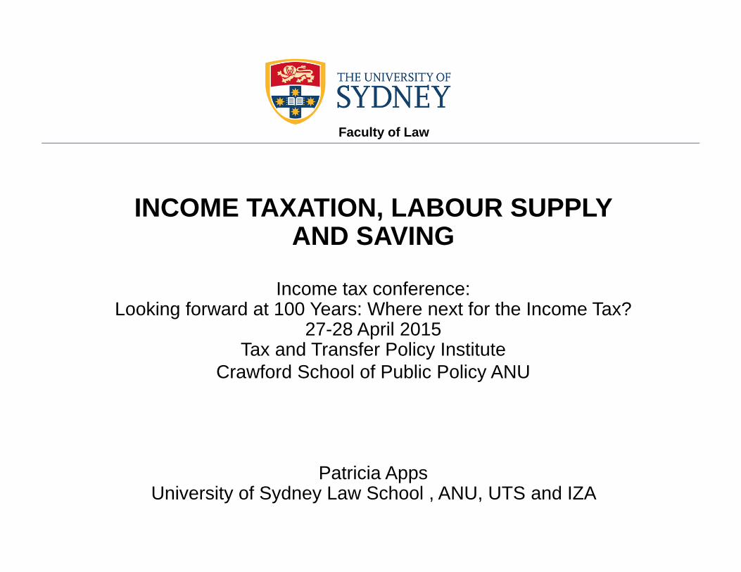
Check with ABS HES 2009‐10 dataPrimary + second income distribution Bracket creep and a revenue neutral GST rise: equally regressive

Why promote GST as a solution to bracket creep?Will we see a further shift in the tax burden to the “middle”?

Faculty of Law

050

100

150

200

250

300

350

Prim

+sec

inco

me,

dol

lars

/100

0

1 2 3 4 5

Prim+sec income quintiles

2013-14 2023-24

 Primary income quintile 1 2 3 4 5 Percentage point rise in ATR 5.91 4.57 4.27 3.71 3.05 GST: ATR% 6.03 4.75 4.13 3.78 2.99

1 Male/primary earner elasticities

Argument for lower tax rates on top incomes usually based on efficiency gains from reduced labour supply disincentive effects. Not supported by cross-section or panel data. Labour supply profile is too flat relative to the profile of wage rates. (Andrienko, Apps and Rees, 2014).

Some economists try to get strongly positive estimates for the top percentiles by switching to gross earnings data, e.g. Brewer et al. (2008) use data for Thatcher years of tax cuts and CEO pay rises and attribute positive estimates to a greater input of “unobservable effort”.

Faculty of Law

050

100

150

200

250

Wag

e

0 10 20 30 40 50 60 70 80 90 100Wage percentile

US UKAU

0.1

.2.3

.4.5

.6.7

.8E

last

icity

0 10 20 30 40 50 60 70 80 90 100Wage percentile

US UKAU

1 Male/primary earner elasticities

Piketty, Saez and Stantcheva (2014):

• low estimates of labour supply elasticities at the top.• fall in gross earnings or taxable income in response to a higher tax rate

is largely a reflection of an increase in tax avoidance and evasion, or to weakened bargaining power and consequently a lower share of rents.

• recommend that tax avoidance and evasion be dealt with directly and not through the tax scale. (See opposite view in “Re:think”)

• recommend a higher top tax rate in response to rising inequality.

Consistent with results for the structure of optimal tax rates in Andrienko, Apps and Rees (2014).

Faculty of Law

2     Family tax system: tax unit change

Transformation of Australia’s family tax system since 1980s.

Early 1980s: families received universal child payments.Howard years saw universal child allowances completely replaced with payments withdrawn on joint income together with a much less progressive PIT rate scale.

Current system: “quasi-joint” family taxation with the highest MTRs applying across average incomes and to the income of the second earner, creating a net-of-tax gender wage gap that makes the continuing gender gap in pre-tax pay rates look insignificant.

Faculty of Law

2  Family tax system: Targeting fallacy

Argument based on “targeting fallacy”: “cost” and revenue savings from reducing “middle class welfare”. Example:

Re:think: “Reducing effective tax rates is not straightforward because reducing the rate at which payments are withdrawn, or removing them altogether, would extend assistance to higher income levels”.

PIT is a piecewise linear income tax: Key lesson of modern tax theory: Individual faces two tax parameters: a marginal rate and a lump sum.

A tax system that gives a transfer and then withdraws it as income rises is equivalent to one with the same universal payment and a new structure of marginal tax rates and lump sums. The relevant basis for evaluating the “cost” of a tax system is not the “universality” of the payment, but the value of the payment and the effect of the structure of MTRs on incentives.

Faculty of Law

2     Female/second earner elasticities 

Higher MTRs on 2nd earners: tax burden shifted to partnered working mothers. Negative impact on female labour supply based on estimates of positive and significant female labour supply elasticities.

Gender gap in labour supply and elasticities emerges after first child.

Additional work choice: One parent, typically the mother on a lower wage, can work at home providing child care and domestic services as an alternative to working in the market and buying in care and related services.

High female labour supply elasticities reflect a high elasticity of substitution between market consumption (child care and related services) and home production (home child care and domestic work). (Note: substitution is notbetween consumption and “leisure”).

Faculty of Law

3 Life cycle time use 

The impact of child care on female labour supply is strongly evident from the time use decisions families make over a life cycle defined not on the age of “head of household” as in the economics literature, but on the presence of dependent children and age of youngest child.

We define the life cycle on five phases:

• Pre-children • At least one child of preschool age is present • Children are of school age or older but still dependent • Parents are of working age but with no dependent children at home• Retirement.

Faculty of Law

3 Life cycle time use: ABS data

5  phases:  1   pre‐child phase – almost identical female and male market hours2   child 0 to 4 phase – dramatic fall in female market hours3   child 5+  phase4   post‐child phase (under 60)5   retirement (60+)

Faculty of Law

010

0020

0030

0040

00M

arke

t hou

rs p

a

1 2 3 4 5Life cycle phase

Male labour supply Female labour supply

010

0020

0030

0040

00D

omes

tic a

nd c

hild

car

e ho

urs

pa

1 2 3 4 5Life cycle phase

Male dom+ccare hrs Female dom+ccare hrsMale domestic hrs Female domestic hrs

3 Life cycle  literature

Life cycle literature treats household as a single person and defines the life cycle on age of “head”. Misreads the data. (For a survey see Attanasio et al. 2010).

The studies find that male and female labour supplies and household consumption initially rise together with age and then fall towards retirement.Labelled the “excess sensitivity puzzle”. Range of theories offered as possible explanations,e.g., “buffer stock” – precautionary saving model, etc.

Approach misses the large fall in female supply that takes place after the arrival of the first child because consumption and labour supplies are averaged across couples in phases 1 and 2.

Faculty of Law

3   Saving tracks female labour supply

Approach also misses the impact of female labour supply on saving.

Median household income, earnings and saving, HES 2009-10

Consumption, household income and saving track female labour supply.

Faculty of Law

Phase

Household income

Female earnings

Saving

1 116141 47502 19760 2 83824 6240 5824 3 110244 30212 9776 4 94744 26208 14040 5 6980 0 1404

 

3 Gender gap in labour supply

Life cycle time use profiles show large gender gap in labour supply.

Female hours are only around half male hours even in phase 4 due to high part time and low full time rates.

Participation rates are misleading – show relatively small gender gap.

High degree of heterogeneity across child rearing phases and phase 4. Data reflect persistence of labour supply decisions made during child rearing years – attributed to loss of human capital.

Faculty of Law

3 Saving heterogeneity

2nd earnings and saving by primary income, phases 2 to 4

H1: 2nd earnings at or below median; H2: 2nd earnings above median

By switching type, from H1 to H2, saving almost doubles.Note: level of saving rises with female labour supply while saving rate falls if female earnings < male earnings. Missed in single-person model.

Data highlight importance of modelling tax reform based on a two-person model of the household.

Faculty of Law

Primary income quintiles 34265 54701 71982 96648 201855H1: 2nd earnings $pa 330 9745 9494 16794 12835 Saving $pa -8227 331 4095 14268 54642H2: 2nd earnings $pa 24425 37410 43001 60451 67281 Saving $pa 297 9075 16167 30634 76973

4 Income vs consumption tax

2015 Treasury Working Paper (TWP): (GE model)

Computes “marginal excess burden” (MEB) of taxes assuming:

• Single-person household with a single labour supply elasticity • Fixed domestic capital or fixed saving rate

as in KPMG (2010, 2011), etc. Typical results:TWP KPMG

Labour income tax MEB ($) 21c 24cBroad-based GST MEB ($) 17c 8cElasticity 0.15 0.20

GST found to be more efficient: fictional result. (See Apps, 2015.)

Faculty of Law

4 Income tax – efficiency merits

A well-designed labour income tax will always be superior to a consumption tax because it is a less constrained policy instrument.

Individual earnings can be observed and taxed progressively, allowing a lower tax rate on the 2nd earner with the more responsive labour supply and higher saving rate at a given wage.

Individual consumptions cannot be observed. We can never observe whose consumption has been reduced to fund household saving

A broad based consumption tax is inevitably a flat rate joint tax. Exempting capital income is inconsistent with the theory of “second-best”, which forms the foundation of the economics of taxation.

Female labour is arguably the most mobile factor of production.

Faculty of Law

4   Labour income tax – equity merits

Progressive individual taxation is superior in terms of horizontal equity as well as vertical equity.

Horizontal equity: a two-earner family working twice the hours of a single-earner family to earn the same joint income pays less tax.

Under Joint taxation – flat rate and progressive – they pay the same amount of tax – inequitable because home production is untaxed.

Household income is an unreliable indicator of living standards in an economy in which wages and earnings are relatively flat across much of the income distribution. ABS data show that when the second partner in a low wage single-earner family goes out to work that family can be reranked from quintile 1 to quintile 4. (See Apps and Rees, 2013.)

Faculty of Law

Concluding comment

Looking forward at 100 Years: Where next for the Income Tax?

Reverse the direction of reform of recent decades:

• Move to more progressive taxation of labour and capital income to deal with rising inequality of income and wealth

• Return to the individual as the tax unit• Deal with tax avoidance and evasion directly, and not through the

tax rate scale (Picketty et al.)

Faculty of Law

ReferencesAndrienko, Y, P Apps and R Rees (2014), “Optimal Taxation, Inequality and Top Incomes”. http://ftp.iza.org./dp8275.pdf

Apps, P (2015), “Expanding the GST Would Hit the ‘Middle’ and Women the Hardest”, The Conversation, http://theconversation.com/expanding‐the‐gst‐would‐hit‐the‐middle‐and‐women‐the‐hardest‐36133

Apps, P and R Rees (2013), “Raise Top Tax Rates, Not the GST”, Australian Tax Forum, 28, 679‐693.

Attanasio, O and G Weber (2010), “Consumption and Saving: Models of Intertemporal Allocation and Their Implications for Public Policy”, Journal of Economic Literature, 48, 693‐751.Australian Government (2015), Re:think,  Tax Discussion Paper.  

Brewer, M , E Saez and A Shephard (2008), “Means‐testing and Tax Rates on Earnings”, paper prepared for the Mirrlees Review, Institute of Fiscal Studies, London.

Cao, L, A Hosking, M Kouparitsas, D Mullaly, X Rimmer, Q Shi, W Stark and S Wende (2015), Understanding the Economy‐Wide Efficiency and Incidence of Major Australian Taxes”, Treasury WP 2015‐01, Australian Government.

Piketty T, E Saez and S Stantcheva (2014), “Optimal Taxation of Top Labor Incomes: A Tale of Three Elasticities”, American Economic Journal: Economic Policy, 6(1), 230‐271.

Faculty of Law