Forecasting Individual

Income Tax Revenues:

A Technical Analysis

Special StudyAugust 1983

CONGRESS OF THE UNITED STATES flHffi CONGRESSIONAL BUDGET OFFICE

FORECASTING INDIVIDUAL INCOME TAX REVENUES:A TECHNICAL ANALYSIS

The Congress of the United StatesCongressional Budget Office

PREFACE

Reliable estimates of federal spending and revenues, and a clearunderstanding of associated issues, are important to the budget process.The Congressional Budget Office (CBO) has developed elaborate techniquesto generate budgetary estimates and to analyze issues affecting spendingand revenue totals. In order that these procedures and issues can beevaluated by those outside the agency, it is CBO's practice to providepublished analyses of its estimating procedures and of current issuesrelated to major spending items and revenue sources. This paper providessuch analysis for individual income tax revenues, the largest singlecomponent of federal receipts.

The study was prepared by Frederick Ribe and Kathleen O'Connell ofCBO's Fiscal Analysis and Tax Analysis Divisions, respectively, under thedirection of Rosemary Marcuss. Mr. Ribe is the principal author. Ms.O'Connell is responsible for parts of Chapters II and IV, and provided expertadvice during all other phases of the project. Others to whom the authorsare grateful for valuable comments are Timothy Considine, EdwardGramlich, Robert Hartman, Frank de Leeuw, Robert Lucke, Steven Malin,Joseph Pechman, and James Verdier. Susan Goeransson, Debra Holt, andNaif Khouri provided research assistance, Patricia H. Johnson edited themanuscript, and Shirley Hornbuckle and Linda Brockman typed it forpublication.

Alice M. RivlinDirector

August 1983

111

CONTENTS

Page

PREFACE iii

SUMMARY ix

Available Revenue Estimating Techniques ixThe CBO Tax Model • ix

The Forecasting Record • xiResponsiveness of Individual Tax

Revenues to Changes in Income xiiEconomic Effects of Indexation- xiii

CHAPTER I. INTRODUCTION 1

How Revenues Are Estimated 1Two-Part Procedures 3

The CBO Model • 4Plan of the Study 5

CHAPTER II. THE CBO INCOME TAX MODEL 7

Overview 7Part 1: Forecast of the Tax Base fromTaxable Personal Income 9

Approach Used in Earlier Studies 9Representation in the CBO Model 10

Part 2: Determining the EffectiveTax Rate 13

How the Effective Tax Rate Worksin the Actual Economy 13

The Structure of Brackets and Rates • • 13How the Tax Base is Spread Over the

Bracket Structure 1*Modeling Movements of Taxable Income

Through the Brackets • 1*Predicting Values of the Effective Tax Rate 19Accuracy of the Model's Tax Rate Reduction 20

Part 3: Predicting Individual Income TaxLiabilities 23

CONTENTS (Continued)

Part 4: Converting Predicted Tax Liabilitiesto Individual Income Tax Revenues 24

Adjustments to Liabilities 24Timing Adjustments 25Adjustments for the Effects of RecentTax Legislation 27

Generating Unified Budget Receipts: A Review 27Forecasting Overall Revenues from theIncome Tax 27

Estimating Revenue Impacts of Changes inTax Policy 28

Further Research • • 29

CHAPTER III. FORECASTING ACCURACY OF THE CBO INDIVIDUALINCOME TAX MODEL 31

Causes of Forecasting Errors 31Three Forecasts with the CBO Model 31

CHAPTER IV. ISSUES IN INDIVIDUAL INCOME TAX REVENUES- - • 35

The Response of Tax Liabilities to Increasesin Income Caused by Inflation 35

Revenue Implications of the Recent Slowdownin Inflation 38

The Revenue Impact of Tax Indexation in 1985 39Economic Implications of Indexation 41

APPENDIX: ANALYSIS OF ERRORS IN TREASURY REVENUEFORECASTS 45

VI

TABLES

TABLE 1. THREE SIMULATED FORECASTS OF REVENUES FROMINDIVIDUAL INCOME TAX USING CBO TAX MODEL • •

TABLE 2. ANALYSIS OF ERRORS IN TREASURY DEPARTMENTFORECASTS OF INDIVIDUAL INCOME TAX REVENUESFOR FISCAL YEARS 1977-1981

TABLE 3. CHANGE IN PREDICTED INDIVIDUAL INCOME TAXREVENUES FROM REVISION IN CBO INFLATIONFORECAST FOR 1983-1986

33

39

FIGURES

FIGURE 1. DISTRIBUTION OF TAXABLE INCOME FOR JOINTRETURNS OVER THE BRACKET STRUCTURE, FORCALENDAR YEARS 1964 and 1979

FIGURE 2.

FIGURE 3.

FIGURE 4.

ACTUAL AND CBO PREDICTED DISTRIBUTIONS OFTAXABLE INCOME FOR JOINT RETURNS OVER THEBRACKET STRUCTURE FOR CALENDAR YEARS 1964AND 1979 AND CBO PREDICTED DISTRIBUTION FORCALENDAR YEAR 1985

15

ACTUAL AND PREDICTED EFFECTIVE TAX RATES,CALENDAR YEARS 1964-1980

21

22

IMPLICIT ELASTICITY OF TAX LIABILITIES WITHRESPECT TO TAXABLE PERSONAL INCOME UNDERINDEXED AND UNINDEXED TAXES, ASSUMINGDIFFERENT RATIOS OF GROWTH IN THE GNPDEFLATOR TO TOTAL NOMINAL GNP GROWTH 36

vn

SUMMARY

Developing budgetary and revenue forecasts to provide assumptionsunderlying congressional concurrent resolutions on the budget is an impor-tant function of the Congressional Budget Office (CBO). This paperdescribes major aspects of the techniques used by CBO to forecastrevenues from the individual income tax: procedural methods, accuracy,comparison with other techniques, and implications about the futurebehavior of individual income tax revenues.

AVAILABLE REVENUE ESTIMATING TECHNIQUES

The most prominent available technique for estimating revenues fromthe individual income tax is the large-scale "microanalytic" model. Thismodel consists mainly of a detailed computer-based miniature replica ofthe taxpaying population of the United States. The revenue implications ofdifferent economic conditions and statutory tax provisions are analyzed bycalculating the effects that they would have on the liabilities of taxpayersin different categories, and then adding these estimates together to predictthe economy-wide impact.

From a practical perspective, large-scale models are versatile andaccurate, but also cumbersome and expensive. These models are especiallyuseful for estimating the revenue implications of changes in tax statutes,which sometimes require detailed analysis that only this technique offers.On the other hand, the elaborate computations of large-scale models aresometimes unnecessary to estimate how revenues change from year to yearin response to changes in economic conditions. In fact, if no significantchanges in tax statutes occur, such year-to-year revenue forecasts aresometimes developed using extremely simple procedures consisting pri-marily of a rule of thumb for predicting growth in taxes on the basis of thegrowth rate of aggregate income. Of course, periods in which the taxstructure is unchanged are rare, especially since enactment of the Eco-nomic Recovery Tax Act of 1981 (ERTA), which mandated a series ofimportant changes in the structure of the income tax over five years.

THE CBO TAX MODEL

CBO's income tax model represents a compromise between therelatively complex and relatively simple alternatives just described. Al-

IX

24-084 0 - 8 3 - 2

though much smaller than large-scale models, it contains enough detail toaccount for the revenue implications of the significant current andprospective changes in the tax structure.

Essentially, the CBO model consists of four equations that deter-mine how important constituent parts of the tax have behaved over longperiods of time. When combined with current institutional information onstatutory tax rates, brackets, and exemption levels, these equations permitforecasts of individual income tax liabilities and federal budget revenuesfrom the individual income tax to be generated on the basis of a separateeconomic forecast of such variables as personal income, employment, andthe price level. The model is designed specifically to account for theeffects of several important recent and current developments on theincome tax. These are:

o Changes in statutory tax bracket rates, such as those entailed inthe Economic Recovery Tax Act of 1981;

o "Bracket creep," or the movement of taxpayers1 incomes upwardthrough the bracket structure as a consequence of inflation orproductivity growth;

o Indexation of statutory tax brackets and the personal exemption,which is scheduled to take effect in 1985; and

o Cyclical swings in aggregate income.

The main advantages of the model are that it is of manageable sizebut still accurate and versatile enough to account for many differenteconomic and legislative developments that affect individual income taxrevenues. Unlike the other forecasting methods, the CBO model is well-documented and open to scrutiny and constructive criticism by taxprofessionals (or anyone else). Moreover, since the CBO procedure isdifferent from most other techniques, it can provide a check on theiraccuracy.

The analysis of overall individual income tax revenues is divided intofour parts. The first part produces an estimate of the tax base (grosstaxpayer income minus all deductions and exemptions) on the basis of aneconomic forecast derived separately by CBO's Fiscal Analysis Division,together with assumptions concerning relevant provisions of the tax code.The economic forecast (covering gross national product (GNP), prices,employment, and other variables) is developed in the Fiscal AnalysisDivision separately from the revenue forecast developed in the TaxAnalysis Division and the outlay forecast in the Budget Analysis Division.The three forecasts are, however, adjusted in light of one another to ensure

consistency. Sometimes several different adjustments are made before afinal set of forecasts is derived.

The second part of the analysis predicts the effective tax rate thatapplies to the tax base developed in Part 1. This computation involvespredicting the pattern by which the tax base will be spread over thestatutory tax bracket structure and how this pattern changes throughbracket creep. By taking detailed account of the statutory characteristicsof the bracket structure, this part of the model permits analyses of variouschanges in statutory bracket boundaries and rates, such as the changesmandated by ERTA.

The third part of the model develops a forecast of aggregate taxliabilities before credits using the results from Parts 1 and 2. Finally, thefourth part generates and incorporates estimates of tax credits and othertax items, and applies timing and other accounting adjustments to the taxliability forecast to derive a forecast of budget revenues from theindividual income tax.

The Forecasting Record

The most important test of the reliability of any forecasting modelis a comparison of the record of its forecasts, together with those ofalternative procedures, to actual data after the forecasting period iscompleted. CBOfs model is quite new, and therefore doesn't have anextensive record. Nevertheless, CBO has developed evidence on themodel's reliability by developing "ex post" (or after the fact) forecasts ofrevenues in past years. This is done by putting oneself in the position of animaginary forecaster several years ago who is using the CBO model toforecast revenues in later years that by now have been observed.

CBO has developed figures comparing the accuracy of ex postforecasts by its tax model with the Treasury Department's publishedindividual income tax revenue forecasts for the same years. Attention isrestricted to forecasting errors caused by technical inaccuracy in theprocedures as opposed to errors resulting from inaccurate assumptionsabout the economy and about the passage of tax legislation affectingrevenues. CBO's average errors for forecasts one, two, and three yearsinto the future were all smaller than CBO's estimates of correspondingTreasury Department errors. Overall, these figures show that the CBOmodel is quite accurate, and compares favorably with alternative proce-dures.

XI

Responsiveness of Individual Income Tax Revenues to Changes in Income

As this discussion has already noted, much interest centers onsummary measures of the response of overall tax revenues to changes inthe economy. Several recent developments, moreover, have altered theresponsiveness of the tax. For example, the ERTA rate cuts that make thetax less progressive by reducing the top rates have likewise made it lessresponsive to economic changes, and the ERTA provision calling forindexation of certain tax provisions to the Consumer Price Index starting in1985 will reduce the responsiveness even more.

The CBO income tax model can be used to calculate the response ofrevenues to different economic developments under various configurationsof the tax laws. For example, under the bracket tax rates that will be ineffect during 1984--following all the reductions that were mandated inERTA—simulations with the model show that the responsiveness of taxliabilities to changes in GNP depends significantly on whether the GNPchange primarily reflects inflation or represents a change in real output.Revenues change more sharply when GNP changes because of inflationrather than other factors. This occurs because increases in GNP resultingfrom inflation alone are taxed at higher rates as taxpayers are pushed intohigher tax brackets. In quantitative terms, individual income tax revenuesmay grow as much as 70 percent faster than GNP if nominal GNP growth isentirely due to inflation.

By contrast, when GNP increases because of an increase in realoutput, some of the resulting income accrues to existing workers as aresult of productivity increases, and this can cause bracket creep for theseindividuals. At the same time, however, much of the increase in aggregateincome accrues to new workers who are drawn into employment by theupswing in the economy. New workers1 incomes are taxed at relatively lowrates, and this makes the responsiveness of income tax revenues to changesin real GNP relatively small. Estimates from the CBO model suggest thatrevenues increase roughly 30 percent faster than GNP when the GNPchange is entirely real.

When the tax structure is assumed to be indexed to the price level,as it will be in 1985 and later years under the terms of ERTA, the tax willbe more responsive to changes in aggregate income that are primarily"real" than to those that reflect inflation. Indexation prevents inflationfrom causing bracket creep, and this reduces the strength of the revenueresponse to inflation. Estimates from the CBO model suggest thatrevenues under the indexed income tax will grow at roughly the same rateas GNP when the GNP change is entirely due to inflation. This is adramatic reduction in responsiveness from that in the unindexed tax, whererevenues are estimated to grow as much as 70 percent faster than income

xn

under the same conditions. Income increases that result from stronggrowth in real output, by contrast, accrue in part to new workers and inpart to existing workers as a consequence of growth in productivity.Productivity growth can cause these workers1 incomes to move into highertax brackets without protection from indexation, which is designed toeliminate bracket creep only when it results from inflation. Thus, somebracket creep may occur in response to real economic growth under theindexed income tax. As a result, CBO estimates that revenues from theindexed income tax will grow 30 percent faster than GNP if the GNPchange is entirely real.

Economic Effects of Indexation

The shift in the behavior of the income tax that will be caused byindexation may have significant implications for the economy. Taxpayerswill gain because indexation will protect them from unlegislated taxincreases caused by inflation-induced bracket creep. Increases in economicefficiency may also result since marginal tax rates will be prevented fromdrifting upward. Indexation could also have adverse impacts, however. Itcould contribute to the tendency of structural budget deficits to increaseover time (in the absence of legislation to control them). The expectationof large and rising deficits, in turn, may help explain the persistently highlevels of interest rates, which may ultimately reduce living standards byreducing investment. Indexation may also reduce the value of the incometax as an automatic stabilizer of the economy.

Xlll

CHAPTER I. INTRODUCTION

A principal responsibility of the Congressional Budget Office (CBO) isto forecast federal revenues and spending in future years under variousassumed budgetary policies and economic conditions. Generating suchestimates can sometimes be an elaborate process for certain revenuesources and spending programs. Because of its complexity, the individualincome tax is one such case. This paper describes the various proceduresthat are available for estimating individual income tax revenue and, inparticular, the nature and forecasting record of CBO's methods.

HOW REVENUES ARE ESTIMATED

Occasionally, when the tax structure is not expected to change,accurate revenue forecasts can be made using simple rules relating thegrowth of tax liabilities to the projected growth in the economy. This ispossible because, during periods in which the tax law has not changed in thepast, the response of individual income tax liabilities to growth in the taxbase has exhibited some regularity.*

The most common summary measure of the response of tax liabilitiesto income changes is the "tax elasticity," expressing the percentage bywhich tax liabilities change for every percentage change in income.Estimates of the elasticity are available from several sources. See,for example, Joseph A. Pechman "Anatomy of the U.S. IndividualIncome Tax," in S. Cnossen, ed., Comparative Tax Studies; Essays inHonor of Richard Goode (North-Holland, 1983). This study reportsestimates based on simulation of a microeconomic model as well asothers based on time-series regression estimates. See also A. Fries, 3.P. Hutton, and P.3. Lambert, "The Elasticity of the U.S. IndividualIncome Tax: Its Calculation, Determinants, and Behavior," Review ofEconomics and Statistics, vol. 64 (1982), which reports estimatescalculated directly using an analytic formula; and Vito Tanzi, "TheSensitivity of the Yield of the U.S. Individual Income Tax and the TaxReforms of the Past Decade," International Monetary Fund StaffPapers, vol. 23 (1976), which reports cross-section regression esti-mates based on data from different states. A number of technicalissues surround the estimation of the tax elasticity. These arediscussed in Chapter IV.

Often, however, changes in the income tax law are contemplated orenacted, and revenue forecasts must take these changes into account. Forexample, the Economic Recovery Tax Act of 1981 (ERTA) set in motion asequence of tax rate cuts in 1981, 1982, 1983, and 1984, and of changes inexemption and tax bracket levels in 1985 and later years. As a result,simple revenue forecasting rules based on an unchanging tax structure arenot of much value.

In order to forecast revenues under such changing tax provisions, taxanalysts sometimes resort to elaborate computer representations of the taxlaw and of the taxpaying population.2 The Treasury Department's TaxCalculator is one such procedure, and others like it are in use by theCongressional Joint Committee on Taxation and under development atCBO. These procedures essentially forecast the taxpaying decisions andcalculations of individual taxpayers—grouped together with others likethem whenever possible—taking into account the details of the tax code.

While these procedures can be accurate, they are also costly andtime-consuming. Moreover, additional problems affecting the accuracy aswell as the manageability of the procedures are introduced by the need togenerate separate forecasts of certain underlying variables. These areeconomic and demographic variables that are not included in the formaleconomic forecast that forms most of the basis for the tax forecast. Forexample, supplemental forecasts are needed of the distribution of income,the number of dependents claimed by different types of taxpayers,itemized deductions, and certain income items like capital gains that arenot covered by the formal forecast of personal income. Forecasts of these

Such models are computer-based samples drawn from the population ofU.S. tax returns, consisting of substantially fewer returns than thenumber actually filed but still representing in a statistically soundmanner the characteristics of the taxpaying population. Differentamounts of total taxable income, different income distributions, anddifferent tax structures can be assumed, and the corresponding aggre-gate tax liabilities calculated by recomputing the taxes due on eachreturn in the sample. This method was developed by Joseph A.Pechman and his associates at the Brookings Institution, and isdescribed in Joseph A. Pechman, "A New Tax Model for RevenueEstimating," in Alan T. Peacock and Gerald T. Hauser eds., Govern-ment Finance and Economic Development (Organization for EconomicCooperation and Development, 1965); and Joseph J. Minarik, "TheMerge 1973 Data File," in Robert H. Haveman and Kevin Hollenbeck,eds., Microeconomic Simulation Models for Public Policy Analysis, vol.1 (Academic Press, 1980). :

items are typically produced using simple rules that may detract from thesophistication and accuracy of the overall procedure. In addition, the needto carry out these supplemental forecasts makes the overall procedure stillmore cumbersome.

Since agencies that are responsible for budgetary revenue forecastsare sometimes called upon to generate many such forecasts in a shortperiod, the detailed procedures that have just been described can beimpractical. Instead, simpler procedures have been developed.

Two-Part Procedures

One simplified approach that is often used by the Treasury Depart-ment involves two separate parts. In the first part, a hypothetical"constant-law11 revenue forecast is made on the assumption that no changein tax structure has taken place. Then, in a second part, this figure iscombined with an estimate of the gain or loss in revenues that is entailedat the forecast level of taxable income by any changes in tax law that haveoccurred. The overall procedure is streamlined because the "constant-law"estimate in the first part is made using simple procedures for estimatingthe response of "constant law" revenues to changes in economic conditions.The forecast of the gain or loss in revenue from a given change in tax lawin the second part of the procedure is made using a separate and moredetailed model like those described in the last section. The overallprocedure is nevertheless simplified because this estimate must only bemade once for a given change in tax law, and then can be used again andagain with minor adjustments as part of the simpler procedure.3

Even an occasional need to resort to a detailed tax model can makethis two-part procedure cumbersome, however. It means, for example,that if a new tax change is proposed for which a revenue-change estimatehas not already been made, the procedure cannot be completed until arevenue-change estimate is made with the detailed model. For this reason,some analysts have developed simplified revenue-change models that aremore nearly self contained. The CBO income tax model is one example.

The revenue change estimate can be adjusted for changes in the under-lying economic forecast using simple rules.

24-084 0 - 8 3 - 3

THE CBO MODEL

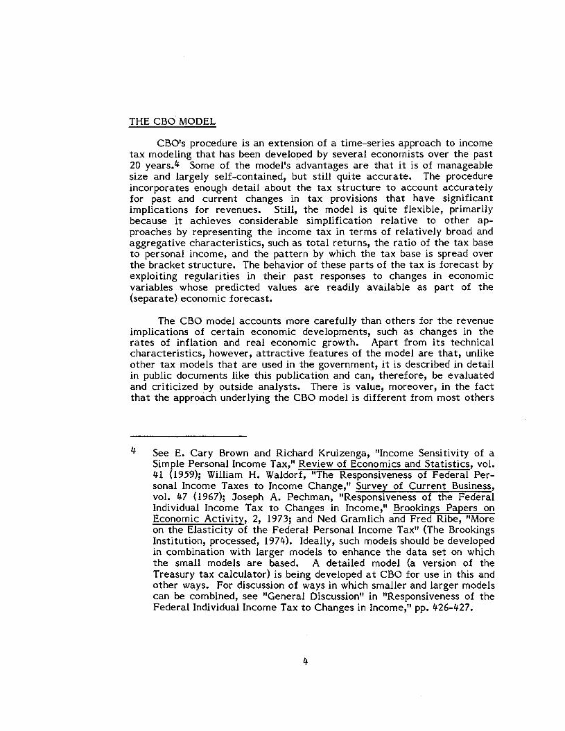
CBO's procedure is an extension of a time-series approach to incometax modeling that has been developed by several economists over the past20 years.^ Some of the model's advantages are that it is of manageablesize and largely self-contained, but still quite accurate. The procedureincorporates enough detail about the tax structure to account accuratelyfor past and current changes in tax provisions that have significantimplications for revenues. Still, the model is quite flexible, primarilybecause it achieves considerable simplification relative to other ap-proaches by representing the income tax in terms of relatively broad andaggregative characteristics, such as total returns, the ratio of the tax baseto personal income, and the pattern by which the tax base is spread overthe bracket structure. The behavior of these parts of the tax is forecast byexploiting regularities in their past responses to changes in economicvariables whose predicted values are readily available as part of the(separate) economic forecast.

The CBO model accounts more carefully than others for the revenueimplications of certain economic developments, such as changes in therates of inflation and real economic growth. Apart from its technicalcharacteristics, however, attractive features of the model are that, unlikeother tax models that are used in the government, it is described in detailin public documents like this publication and can, therefore, be evaluatedand criticized by outside analysts. There is value, moreover, in the factthat the approach underlying the CBO model is different from most others

See E. Gary Brown and Richard Kruizenga, "Income Sensitivity of aSimple Personal Income Tax," Review of Economics and Statistics, vol.41 (1959); William H. Waldorf, "The Responsiveness of Federal Per-sonal Income Taxes to Income Change,11 Survey of Current Business,vol. 47 (1967); Joseph A. Pechman, "Responsiveness of the FederalIndividual Income Tax to Changes in Income," Brookings Papers onEconomic Activity, 2, 1973; and Ned Gramlich and Fred Ribe, "Moreon the Elasticity of the Federal Personal Income Tax" (The BrookingsInstitution, processed, 1974). Ideally, such models should be developedin combination with larger models to enhance the data set on whichthe small models are based. A detailed model (a version of theTreasury tax calculator) is being developed at CBO for use in this andother ways. For discussion of ways in which smaller and larger modelscan be combined, see "General Discussion" in "Responsiveness of theFederal Individual Income Tax to Changes in Income," pp. 426-427.

that are in active use in policy analysis; it therefore provides a check onthe reasonableness and accuracy of those procedures.

PLAN OF THE STUDY

Chapter II describes the CBO model in detail. Chapter III providesevidence on the accuracy of the model's forecasts, and Chapter IV presentsestimates from the model bearing on current issues in federal revenues.

CHAPTER II. THE CBO INCOME TAX MODEL

This chapter describes CBO's revenue forecasting model for theindividual income tax and how it is used. This model was developed forCBO's use in making five-year forecasts of federal budget revenues basedon current tax policy. These forecasts are considered by the Congress indeveloping concurrent resolutions on the budget.

OVERVIEW

The model is designed to account explicitly for the effects of importantcurrent developments affecting income tax revenues. These include:

o Cyclical swings in aggregate income;

o "Bracket creep," the movement of taxpayers1 incomes upwardthrough the progressive tax bracket structure as a consequence ofinflation and productivity growth;

o Changes in statutory tax bracket rates, such as those enacted aspart of the Economic Recovery Tax Act of 1981 (ERTA);

o Indexation of statutory tax brackets, personal exemptions, and thestandard deduction, which was also enacted as part of ERTA totake effect in 1985.

Revenue forecasts by this model are based upon—that is, they take asgiven, or "exogenous"—forecasts by CBOfs Fiscal Analysis Division ofmacroeconomic variables, such as real GNP, the levels of wages and prices,employment, and other variables. 1 Similarly, values for all statutory taxprovisions are specified outside the model.

After a preliminary revenue forecast is made by the Tax AnalysisDivision, the Fiscal Analysis Division reviews its forecast of GNP,taxable personal income, and other National Income and ProductAccounts variables in light of the revenue forecast to ensure that thetwo are consistent. If necessary, revisions are made in the economicfigures. This process of adjustment of the economic forecast to therevenue projection is sometimes repeated several times.

The model itself consists of four parts. The first develops a forecastof the tax base—the narrow Internal Revenue Service 'Taxable Income11

measure—from the forecast of the broader taxable personal income aggre-gate in the National Income and Product Accounts (NIPA).2 This partrepresents the effects of exemptions and deductions in shielding personalincome from taxation and accounts for definitional differences betweenthe tax base and NIPA personal income. The second part derives aweighted-average tax rate that applies to the tax base. This involvespredicting the way in which the tax base is spread over the structure ofstatutory tax brackets and combining this prediction with detailed informa-tion on statutory tax rates. The third part of the model represents thederivation of tax liabilities by combining the tax base from the first partwith the weighted-average tax rate derived in the second part. Since taxliabilities differ from individual income tax revenues collected by thegovernment because of the timing of tax collections and other factors, thefinal part of the model adjusts the liability forecast for these factors,yielding a forecast of federal revenues.

This model, while quite detailed and complex, is intended to accountdirectly only for economic and policy developments with major conse-quences for tax revenues. Tax policy measures with smaller revenueimplications must be analyzed separately and their revenue consequencesadded to the projections of the main model. Examples of measures thatcurrently must be handled separately are changes in capital gains taxprovisions and changes in Individual Retirement Account and Keogh planprovisions, among others. Over time, these specific items become incor-porated in the estimation of the tax base, but at any point in time recentlylegislated tax provisions with smaller revenue effects are handled separ-ately.

Each of the four main parts of the model is estimated on the basis ofhistorical data, and is described below in turn. All logs are natural logs.

Taxable personal income (TPY) consists of wage and salary disburse-ments, personal interest income, personal dividend income, rentalincome of persons, and farm and nonfarm proprietors1 incomes. Equiv-alently, TPY can be computed as personal income minus governmenttransfer payments and other labor income plus personal contributionsfor social insurance. Since transfers are excluded and personalcontributions for social insurance are included, TPY is the same asPechman's "adjusted personal income". See "Responsiveness of theFederal Personal Income Tax to Changes in Income," p.

PART 1: FORECAST OF THE TAX BASE FROM TAXABLEPERSONAL INCOME

Approach Used in Earlier Studies

In computing tax liabilities, each taxpayer first subtracts fromadjusted gross income a set of "exclusions": one or more personal exemp-tions and either a "standard" deduction ("zero bracket amount") or a set ofitemized deductions. What remains is taxable income, or the "tax base" forthat taxpayer.

Most tax models, including that of CBO, analyze this process at theaggregate level, relating the total tax base in the economy to total grossincome as well as to variables accounting for changes in the relevantprovisions of the tax law. This is simpler than analyzing the decisions ofindividual taxpayers or groups of taxpayers, and is still quite accurate.

As an additional simplifying step, proxy variables are often used foraggregate adjusted gross income, aggregate itemized deductions, and totaltax returns. This procedure is used because none of these variables isnormally predicted by formal economic forecasting procedures, and at-tempts to forecast them separately may not improve the accuracy of theoverall analysis of the tax base.

Several earlier studies have used personal income from the NIPA as aproxy for adjusted gross income and total population as a proxy for totalreturns.3 Itemized deductions, for their part, have been assumed to beproportional to aggregate gross income so no separate proxy variable isneeded.* The earlier studies then predict the fraction of aggregate grossincome that appears in the narrower aggregate tax base in terms of thelevels of gross income per tax return, capital gains per return, thestatutory personal exemption, and the statutory standard deduction (zero

See "Income Sensitivity of a Simple Personal Income Tax," "TheResponsiveness of Federal Personal Income Taxes to Income Change,"and "Responsiveness of the Federal Individual Income Tax to Changesin Income."

In addition to the studies cited in footnote 3, this assumption is madein "The Elasticity of the U.S. Individual Income Tax: Its Calculation,Determinants, and Behavior." Other analysts have pointed out,however, that the assumption is sometimes violated in practice andthat the behavior of the tax can be affected significantly. See DavidGreytak and Richard McHugh, "Inflation and the Individual IncomeTax," Southern Economic Journal, 45 (1978).

bracket amount). Once the fraction of gross income appearing in the taxbase has been determined, it is a simple matter to compute the predictedlevel of the tax base itself.

Each of the explanatory variables used in these studies should beexpected a priori to have an identifiable qualitative effect on the ratio ofthe tax base to gross income. Other factors being equal, increases ineither the personal exemption or standard deduction should reduce theratio, while increases in gross income per return should increase it. Thissecond effect should occur because increases in income per return mayaccrue largely to existing taxpayers and thus may not be as well protectedfrom taxation by exemptions and deductions as increases that accrue tonew taxpayers. A greater proportion of an income increase accruing toexisting taxpayers should, therefore, enter the tax base.

Representation in the CBO Model

The CBO model, like earlier studies, generally follows the approachoutlined above. Like most earlier treatments, for example, the modelassumes aggregate itemized deductions to be proportional to gross income.The CBO approach departs from the earlier studies in important ways,however. In particular, the CBO model uses total employment instead ofpopulation as a proxy for total returns, and taxable personal income fromthe NIPA instead of personal income as a proxy for aggregate adjustedgross income. Employment, like population, is easily forecast; it isroutinely included, in fact, in economic forecasts developed at CBO.Unlike population, however, employment varies over the business cycle.Since total tax returns also exhibit such variation, using employment ratherthan population prevents the model from overlooking important cyclicalaspects in the behavior of returns, as is done in other studies.^ Taxable

In particular, this treatment implies that changes in aggregate grossincome that reflect price increases alone are taxed more heavily thanare changes in aggregate real income. This is because changes in realincome change employment and the number of tax returns. Incomeper return, therefore, changes less quickly when the income change isreal than when it is purely nominal. The quantitative implications ofthis and other properties of the CBO model are described in ChapterIV.

10

personal income, similarly, is a closer proxy for adjusted gross income thanis personal income, and is also routinely included in CBO economicforecasts.6

The estimated equation that results from all these considerations,using historical time-series data for 1954-1980, is

(1) log ( Z ) = -2.16473 - .25983 (log (TPY) - log (ESTAT))(TFY) (-18.91) (-10.35) (EMP)

-.05442 (log (TPY) - log (SDSTAT))(-2.846) (EMP)

-.03002 log (CG )(-2.054) (EMP)

-.02311 D6469(-2.178)

- .01980 D7076(-2.609)

R2 = .9809Standard error =.01369Durbin-Watson statistic = 1.3985Sample period = 1954-1980 (annual data)(Numbers in parentheses are t-statistics)

Another modification relative to earlier papers is more technical. Ifincreases in taxable personal income per return that are accompaniedby increases at the same rate in the personal exemption and deduction(as, for example, under the indexed tax in the face of "pure" inflationin which all prices and wages rise at the same rate), it is reasonable toexpect that the tax base should rise at the same rate as taxablepersonal income. With this concern in mind, the coefficient of the logof taxable personal income per employee was constrained to be equalto minus the sum of the coefficients of the logs of the exemption andstandard deduction. The implicit coefficient for log (TPY/EMP) in theestimate shown below is .31425, which differs by .00091 from its valuewhen estimated freely. As this result suggests, the constraint on thiscoefficient appeared not to be binding: an F test rejects at the 99percent confidence level the hypothesis that the coefficient of log(TPY/EMP) is not equal to minus the sum of the coefficients of log(ESTAT) and log (SDSTAT).

1124-084 0 - 8 3 - 4

Z is taxable income under the individual income tax (the tax base,IRS definition). To ensure consistency with data for earlier years,the figures exclude the zero bracket amount in 1977-1980. (Source:Internal Revenue Service, Statistics of Income; Individual Income TaxReturns, annual issues.)

TPY is Taxable Personal Income (wage and salary disbursements pluspersonal interest income, personal dividend income, rental income ofpersons, and farm and nonfarm proprietors1 incomes.) (Source:National Income and Product Accounts.)

EMP is total employment (household survey). (Source: Bureau ofLabor Statistics.)

ESTAT is the statutory per capita exemption (Source: InternalRevenue Service, Statistics of Income; Individual Income Tax Re-turns, annual issues.)

SDSTAT is 50 percent of the statutory maximum per-return standarddeduction for joint returns (the zero-bracket amount in 1977-1980).(Source: Internal Revenue Service, Statistics of Income: IndividualIncome Tax Returns, annual issues.)

CG is net capital gains. (Source: Internal Revenue Service, Statisticsof Income: Individual Income Tax Returns, annual issues.)

D6469 is a dummy variable that accounts for the presence of theminimum standard deduction during the period 1964-1969.

D7076 is a dummy accounting for the introduction of the low-incomeallowance during 1970-1976.

This equation does well at explaining the past behavior of the tax base.This is attested by the R2 statistic, which indicates that the equationexplains 98.09 percent of the variation in the tax base as a proportion oftaxable personal income. In addition, all of the a priori theoreticalsuppositions listed above regarding the effects of changes in particularexplanatory variables are confirmed by the estimated coefficients.

12

PART 2; DETERMINING THE EFFECTIVE TAX RATE

How the Effective Tax Rate Works in the Actual Economy

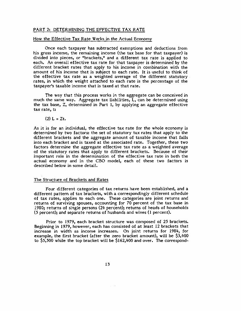
Once each taxpayer has subtracted exemptions and deductions fromhis gross income, the remaining income (the tax base for that taxpayer) isdivided into pieces, or "brackets," and a different tax rate is applied toeach. An overall effective tax rate for that taxpayer is determined by thedifferent bracket rates that apply to his income in combination with theamount of his income that is subject to each rate. It is useful to think ofthe effective tax rate as a weighted average of the different statutoryrates, in which the weight attached to each rate is the percentage of thetaxpayers taxable income that is taxed at that rate.

The way that this process works in the aggregate can be conceived inmuch the same way. Aggregate tax liabilities, L, can be determined usingthe tax base, Z, determined in Part 1, by applying an aggregate effectivetax rate, t:

(2) L = Zt.

As it is for an individual, the effective tax rate for the whole economy isdetermined by two factors: the set of statutory tax rates that apply to thedifferent brackets and the aggregate amount of taxable income that fallsinto each bracket and is taxed at the associated rate. Together, these twofactors determine the aggregate effective tax rate as a weighted averageof the statutory rates that apply to different brackets. Because of theirimportant role in the determination of the effective tax rate in both theactual economy and in the CBO model, each of these two factors isdescribed below in some detail.

The Structure of Brackets and Rates

Four different categories of tax returns have been established, and adifferent pattern of tax brackets, with a correspondingly different scheduleof tax rates, applies to each one. These categories are joint returns andreturns of surviving spouses, accounting for 70 percent of the tax base in1980; returns of single persons (24 percent); returns of heads of households(5 percent); and separate returns of husbands and wives (1 percent).

Prior to 1979, each bracket structure was composed of 25 brackets.Beginning in 1979, however, each has consisted of at least 12 brackets thatincrease in width as income increases. On joint returns for 1984, forexample, the first bracket (after the zero bracket amount), will be $3,400to $5,500 while the top bracket will be $162,400 and over. The correspond-

13

ing schedule of tax rates will rise from 11 percent on the first bracket to50 percent on the last.

How the Tax Base is Spread Over the Bracket Structure

A relatively large percentage of all taxable income falls into thelowest brackets, while increasingly little falls into the higher ones. This isbecause every taxpayer—including those with high incomes—has someincome taxed in the first bracket. Less and less income falls into eachsucceeding bracket because the incomes of lower-income taxpayers gradu-ally are exhausted and do not reach the higher brackets. As a result, thepercentage spread of the aggregate tax base over the bracket structure hasa triangular shape: it is high for the low brackets and low for the high ones(see Figure 1).

Inflation and productivity growth can bring about an increase in thepercentage of total taxable income that appears in the upper brackets ofany given category of returns, and a corresponding decline in the percent-age appearing in the lowest brackets. Figure 1 provides an illustration ofthe way this process has worked in the past. The figure shows the bracketstructure for joint returns in 196* and 1979, together with "curves" showingthe percentage of all taxable income on joint returns that appeared in eachbracket in each of those years. In 1979, the curve was higher for theupper brackets and lower in the bottom brackets.

Modeling Movements of Taxable Income Through the Brackets

It is important to capture the effects of such income movementswhen forecasting individual income tax revenues. Changes in the rate atwhich incomes move into higher brackets affect the weights that areassociated with different statutory tax rates, with significant implicationsfor the weighted-average tax rate, and, consequently for income taxrevenues. In order to explain and predict this process in a tax model, ameans is needed first to replicate the distribution of the tax base over thebracket structure (shown in Figure 1) and then to account for the wayeconomic and statutory factors cause it to change. Fortunately, amathematical tool, the distribution function, is available and is well suitedto this job.

A mathematical distribution function is a formula for a curve likethose shown in Figure 1. Such formulas typically involve only a fewvariables, or "parameters," that must be assigned particular values in orderto determine the full distribution explicitly. If a distribution function canbe found that fits the actual spread of the tax base in different years

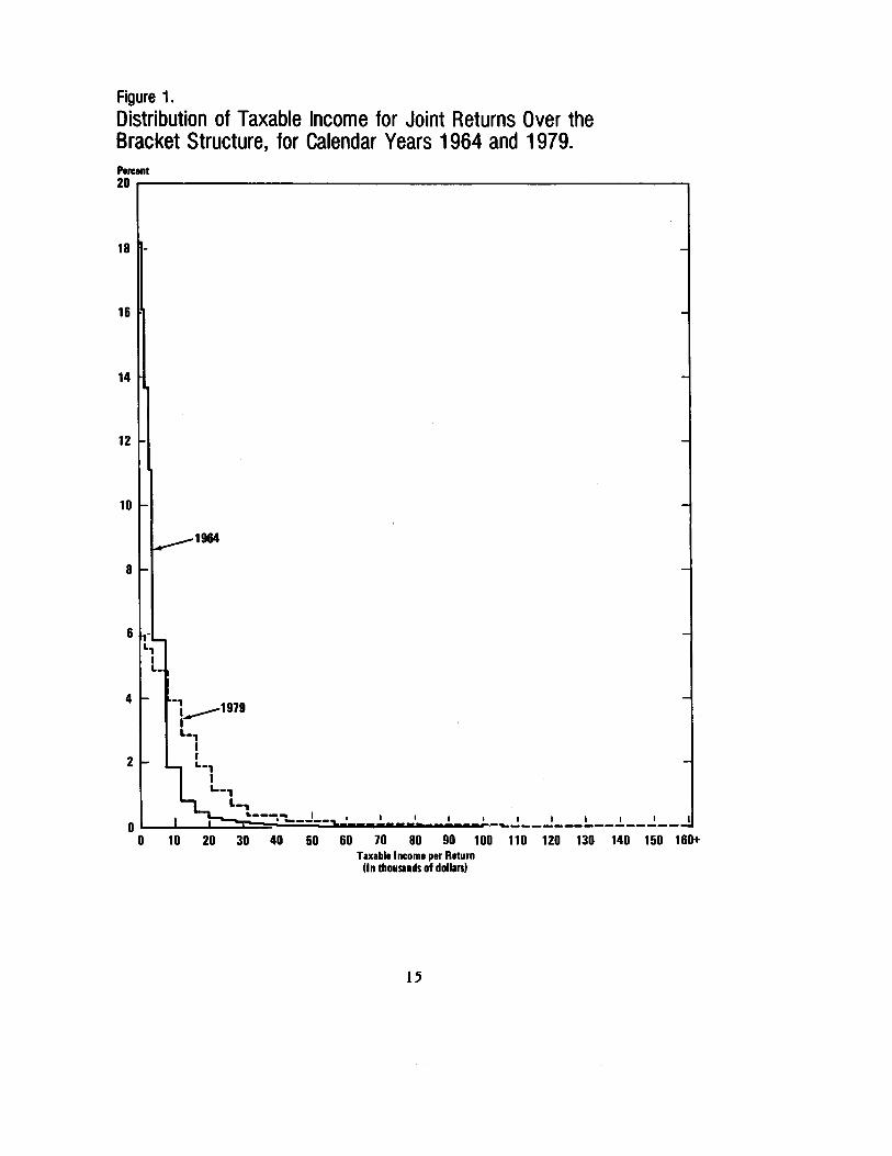
Figure 1.Distribution of Taxable Income for Joint Returns Over theBracket Structure, for Calendar Years 1964 and 1979.Percent20

18

16

14

12

10

^1964

-1979

-1iL.

I

10 20 30 40 50 60 70 80 90 100 110 120 130 140 150 160+Taxable Income per Return

(In thousands of dollars)

15

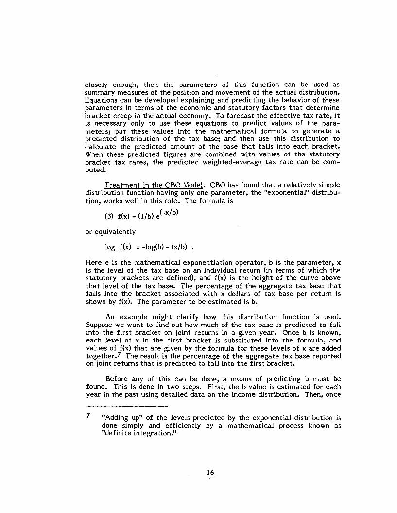
closely enough, then the parameters of this function can be used assummary measures of the position and movement of the actual distribution.Equations can be developed explaining and predicting the behavior of theseparameters in terms of the economic and statutory factors that determinebracket creep in the actual economy. To forecast the effective tax rate, itis necessary only to use these equations to predict values of the para-meters; put these values into the mathematical formula to generate apredicted distribution of the tax base; and then use this distribution tocalculate the predicted amount of the base that falls into each bracket.When these predicted figures are combined with values of the statutorybracket tax rates, the predicted weighted-average tax rate can be com-puted.

Treatment in the CBO Model. CBO has found that a relatively simpledistribution function having only one parameter, the "exponential" distribu-tion, works well in this role. The formula is

(3) f(x) =

or equivalently

log f(x) = -log(b) - (x/b) .

Here e is the mathematical exponentiation operator, b is the parameter, xis the level of the tax base on an individual return (in terms of which thestatutory brackets are defined), and f(x) is the height of the curve abovethat level of the tax base. The percentage of the aggregate tax base thatfalls into the bracket associated with x dollars of tax base per return isshown by f(x). The parameter to be estimated is b.

An example might clarify how this distribution function is used.Suppose we want to find out how much of the tax base is predicted to fallinto the first bracket on joint returns in a given year. Once b is known,each level of x in the first bracket is substituted into the formula, andvalues of f(x) that are given by the formula for these levels of x are addedtogether. 7 The result is the percentage of the aggregate tax base reportedon joint returns that is predicted to fall into the first bracket.

Before any of this can be done, a means of predicting b must befound. This is done in two steps. First, the b value is estimated for eachyear in the past using detailed data on the income distribution. Then, once

"Adding up" of the levels predicted by the exponential distribution isdone simply and efficiently by a mathematical process known as"definite integration."

16

this series of past b values has been developed, it is used to estimate anequation that explains and predicts the behavior of b in terms of othervariables.

In the first step, a b value was determined for each year during the1964-1979 period, using a standard statistical procedure—the maximumlikelihood estimator.8 The second step mainly involved choosing the mostappropriate other variables for determining how b behaves.

The most important factor in explaining the movement of the taxbase through the bracket structure (represented by changes in b) seemslikely to be aggregate income per tax return.9 A good proxy for this

The Internal Revenue Service has decided not to publish data on thisdistribution for 1978, 1980, and apparently for subsequent even-numbered years. Adequate information is, however, available in theannual figures published for 1977 and prior years and the semiannualdata that will be published subsequently. For discussion of ways to fitand analyze income distribution functions, see Charles Metcalf, AnEconometric Model of the Income Distribution (Chicago: Markham,1972); A.B.Z. Salem and T.D. Mount, "A Convenient DescriptiveModel of Income Distribution: The Gamma Density," Econometrica,vol. 7* (197*), pp. 1115-1127; and N.A.J. Hastings and 3.B. Peacock,Statistical Distributions (New York: Wiley, 1974). The treatment inthis paper is not based on a formal representation of the underlyingfrequency distribution of taxable personal income. The formal distri-bution function that is used here represents not the frequency distribu-tion of personal incomes, but the percentage of all taxable incomethat appears at a given per return taxable income level on tax returns.In fitting the exponential distribution, the dollar amounts in terms ofwhich the statutory tax brackets are defined were expressed in unitsof $100,000. The mean of the actual distribution in each year wascomputed by multiplying the lower boundary of each bracket by thepercentage of all of the tax base reported on that type of returns thatwas in that bracket. Then the mean was computed as a weightedaverage by adding together the figures for all the different brackets.The data on amounts of the tax base falling in different brackets arereported in annual issues of U.S. Treasury Department, InternalRevenue Service, Statistics of Income: Individual Income Tax Returns.For figures for joint returns in 1979, for example, see p. 97, column23.

The distribution of the tax base over the bracket structure (of which bis the mean) is related to, but not equivalent to, the conventionalfrequency distribution of income (of which per capita income is the

17

variable, in turn, is some measure of per capita income. This is simplybecause such movement results directly from changes in per capita income.(Variations in per capita income, in turn, are explained or determined byinflation, real economic growth, and other economic developments that areoutside the scope of the tax model.) Using the ratio of the aggregate taxbase, Z, to total employment, for example, CBO has estimated thefollowing equations to explain b:

(4) log(bjr) = -3.36733 + .68414 log (_Z)(-18.96) (10.95) (EMP)

+ . 11996 log (CGJ- .16990 D6469(2.982) (EMP) (-4.023)

- .06396 D7076(-2.514)

R2 = .9929Standard error = .02422Durbin- Watson Statistic = 1.7071

(5) log(bsr) = -4.09986 + .64559 log ( Z )(-20.57) (7.089) (EMP)

Footnote Continuedmean). For this reason, use of per capita income to explain b is nottautological, as it might at first appear. The relationship between thetwo distributions is close enough, however, that factors that increasethe mean of one also increase that of the other. In particular, one ofthe main hypotheses of this paper is that inflation increases the meansof both distributions more strongly than do cyclical increases in realGNP. This hypothesis is supported in a qualitative way with respect tothe frequency distribution by at least one formal study. See A.B.Z.Salem and T.D. Mount, "A Convenient Model of Income Distribution:The Gamma Density," Econometrica, vol. 74 (1974). The argumenthere is also consistent with empirical evidence developed by CharlesMetcalf on the behavior of the distribution of income among familiesin which both spouses are in the labor force. See Charles E. Metcalf,"The Size Distribution of Personal Income During the Business Cycle,"American Economic Review, vol. 59 (1969). Metcalffs evidence forother components of the population, however, is only partially consis-tent with the present argument, as is that in Lester Thurow, "Analy-zing the American Income Distribution," American Economic Review,vol. 60 (1970); and Joseph 3. Minarik, "The Size Distribution of IncomeDuring Inflation," Thie Review of Income and Wealth, 4 (1979).

18

- .20*67 D6*69 - .1088* D7076(-2.600) (-2.178)

R2 = .967*Standard error = .0*765Durbin-Watson Statistic = .9**7

Estimation period: 196*-1979 (annual data); data for 1978 areexcluded because figures for that year are unavailable. (Figures inparentheses are t-statistics.)

bjr is the maximum likelihood estimate of the b parameter for jointreturns. (Source: calculations described in text. For purposes of thiscomputation, income per return is expressed in units of $100,000.)

bsr is the maximum likelihood estimate of the b parameter forreturns of single persons. (Source: calculations described in text.)

Z is IRS Taxable Income. (Source: Internal Revenue Service, Statis-tics of Income: Individual Income Tax Returns, annual issues.)

EMP is total employment, (household survey). (Source: Bureau ofLabor Statistics.)

CG is net capital gains. (Source: Internal Revenue Service, Statisticsof Income; Individual Income Tax Returns, annual issues.)

D6*69 is a dummy variable that accounts for the presence of theminimum standard deduction during the period 196*-1969

D7076 is a dummy variable accounting for the introduction of thelow-income allowance during 1970-1976.

Predicting Values of the Effective Tax Rate

The above analysis is sufficient to permit predictions of the aggre-gate effective tax rate to be made. First, predicted values of the tax base,Z, drawn from equation (1) are substituted with actual values for employ-ment, EMP, in equations (*) and (5). These yield predictions of the bparameters determining predicted distributions of taxable income for jointand nonjoint returns. The distribution for each type of return in each yearis given explicitly by equation (3) after the b value for that type and year issubstituted. The predicted bracket weights (percentages of taxable incomepredicted for each bracket) are then computed taking into account thestatutory boundaries of each bracket. Combining these predicted weights

19

with the corresponding statutory tax rates yields the predicted effectivetax rate for each of these two types of returns.

A final step in computing the effective rate is combining theseparate effective rates computed above for joint and nonjoint returns toform an overall effective rate. This is done by computing a weightedaverage of the two rates, in which the weights are a percentage of theaggregate tax base that appeared on joint returns in a given year, and oneminus this percentage, respectively.

Accuracy of the Model's Tax Rate Predictions

How accurate is this method of predicting weights and rates? TheCBO predicted distributions for joint returns in 1964 and 1979 are shownwith the actual data in panels one and two of Figure 2.10 The fit is notprecise, but the change over time in the predicted distribution correspondsto that of the actual data. Panel three of Figure 2 shows the model'sprojection of how the distribution will look in 1985 (based on a recent CBOprojection of economic conditions in that year.) The outward shift in theprofile continues according to the projections, despite the fact that recentand projected inflation rates are significantly lower than they had been.

Figure 3 presents the actual and CBO predicted effective tax ratesfor 1964-1980. The predicted rate is based on the predicted distributionand actual tax bracket rates. The predicted and actual tax rates moveclosely together. Both series drop in 1965 as a result of the "Kennedy" taxrate cut, and in 1979 as a result of the Revenue Act of 1978. They riseduring 1968-1970 because of the Vietnam surtax, and otherwise show arising trend reflecting bracket creep. The predicted rate falls below theactual rate by a consistent percentage, resulting from the fact that thedistribution function underpredicts the percentages of taxable income thatfall into the upper brackets. Part 3 of the model is able to correct for thisproblem, as the next section shows.

The most important test of the accuracy of the predicted tax rate asa representation of the actual rate, however, is the closeness with which it

The exponential distribution actually slopes continuously downward. Itis represented as a step function in the figure to facilitate comparisonwith the actual percentages. The step function shown for theexponential distribution was derived by computing the percentageimplied by the function for each bracket and then spreading thispercentage uniformly over the bracket.

20

Figure 2.Actual and CBO Predicted Distributions of Taxable Income forJoint Returns Over the Bracket Structure for Calendar Years 1964and 1979 and CBO Predicted Distribution for Calendar Year 1985.Percent20

Actual and CBO Predicted Distributions for 1964

18

16

14

12

10

8

6

4

2

-Actual

-Predicted

Percent10

_L

Actual and CBO Predicted Distributions for 1979

CBO Predicted Distribution for 1985

i i i20 30 40 50 60 70 80 90 100 110 120 130 140 150 160+

Taxable Income per Return(In thousands of dollars)

21

Figure 3.Actual and Predicted Effective Tax Rates, Calendar Years 1964-1980.Percent25

24

23

22

21

20

19

18

Predicted

I 1 I I J I J I1964 1966 1968 1970 1972

Calendar Years1974 1976 1978 1980

22

explains the historical behavior of tax liabilities. The evidence on thisscore is presented in the next section.

PART 3; PREDICTING INDIVIDUAL INCOME TAX LIABILITIES

Once the weighted-average tax rate has been estimated in Part 2,developing a means of predicting tax liabilities involves using the predictedtax rate in place of f f t f f in equation (2) and estimating that equation usinghistorical time-series data. Making this estimate permits a test to bemade of the quality of the estimated weighted-average tax rate as anapproximation of the true rate. The estimate also permits certain otherfactors that affect the relationship between the tax base and tax liabilitiesto be taken into account. The results, in logarithmic form for 1954-1980,11 are

(6) log (L) - log (WRP) = -.00867 + 1.00813 log (Z)(-.3680) (245.0)

-.08795 D5463 - .02451 D70(-23.48) (-6.156)

R2 = .9999Standard error = .00517Durbin-Watson Statistic = 1.6774Sample period = 1954 to 1980 (annual data)(Figures in parentheses are t-statistics)

In this form, the percentage response of tax liabilities to percentagechanges in the predicted effective tax rate from Part 2 is constrainedto equal its expected one-to-one value in order to focus on thepercentage response of liabilities to the tax base. This response alsohas an a priori expected value of unity if the predicted average taxrate is an adequate representation of the actual tax rate. Consequent-ly, whether or not the liability-tax base relationship does turn out tobe unity is a test of the adequacy of the predicted tax rate. A formalstatistical "t" test of this proposition confirms that one can concludewith 99 percent confidence that the response of liabilities to the taxbase takes its expected 1.0 value. Consequently, the predictedeffective tax rate can be inferred to be a good representation of theactual rate.

23

L is individual income tax liabilities before credits. (Source: InternalRevenue Service, Statistics of Income: Individual Income Tax Re-turns, annual issues!)

WRP is the predicted weighted-average tax rate. (Source: computa-tions described in text.)

Z is IRS taxable income. (Source: Internal Revenue Service, Statis-tics of Income: Individual Income Tax Returns, annual issues.)

D5463 is a dummy variable accounting for the discontinuous behaviorof the effective tax rate during the sample period; the rate wasinexplicably stable before 1964. Accordingly, this variable takes thevalue unity before 1964 and zero thereafter. The fit of this equationis not significantly changed if the sample period is confined to 1964-1979, permitting this dummy to be dropped.

D70 is a dummy variable accounting for the effects of the TaxReduction Act of 1970 in changing the percentage of taxable incomethat appeared on nontaxable returns. It also accounts for a minorinconsistency in the data for L before and after 1970; before thatyear, these figures are net of small amounts of tax credits, but theyare gross of all credits in 1970 and later years. D70, accordingly, iszero before 1970 and unity subsequently.

The dummy variable for 1954-63 helps offset the fact noted abovethat the predicted effective tax rate WRP systematically understates theactual rate. The overall result is satisfactory, as is shown by the R2statistic, whose value in this case is .9999. That figure states that theequation explained all of the variation in tax liabilities during the sampleperiod. The equation, therefore, seems likely to forecast accurately,though a more direct test is the record of accuracy of actual forecasts bythe complete model. This record is described in the next chapter.

PART 4; CONVERTING PREDICTED TAX LIABILITIES TO INDIVIDUALINCOME TAX REVENUES

Projections of income tax liabilities described above do not indicatethe amount of revenue that will be available to the government in a givenbudget cycle. Several additional computations must be made in order toproduce an estimate of fiscal year individual income tax receipts. Thesecomputations fall into three categories: adjustments to liabilities forcredits and additional taxes for tax preferences, adjustments for the timingof tax payments, and adjustments for the effects of recent tax legislation.

24

Adjustments to Liabilities

The measure of liabilities used thus far in the CBO model, liabilitiesbefore credits, is the appropriate measure for calculating the amount oftax generated by the assumed levels of income and characteristics of thetaxpaying population. It is not, however, a measure of total income taxliabilities. Because some taxpayers are allowed credits against the amountof taxes owed and some taxpayers are required to pay tax additional to theamount resulting from the standard tax calculations, adjustments must bemade to account for these items.

Tax credits are allowed for a variety of reasons. The earned incomecredit is intended as relief for low-income taxpayers with dependentchildren; other credits, such as the investment credit and the jobs creditare intended to encourage certain kinds of behavior on the part of sometaxpayers. Because total tax credits bear a stable relationship to overallincome, CBO projects the aggregate amount of credits using a trend basedon recent tax credit experience. The estimate of liabilities before creditsdeveloped in Part 3 is reduced by this amount.

An additional adjustment is made to liabilities to account for thepayment by some taxpayers of a minimum tax on certain income anddeduction items they claim on their tax return. Because the preferentialtreatment of these items results in lower taxable income and, therefore,lower tax liabilities, these items are designated in the tax code as "taxpreferences.11 Taxpayers who claim these items are required to pay aminimum of 15 percent tax on the amounts, computed according to IRSrules. Because the total "additional tax for tax preferences" has, forseveral years, followed the same pattern as total net capital gains, CBOprojects these additional taxes on the basis of projected capital gains, usingthe most recently observed ratio of these two variables. The projectedamount of additional tax for tax preferences is then added to liabilitiesbefore credits. These adjustments are summarized below.

Total Income Tax Liabilities = Liabilities Before Credits- Total Tax Credits+ Additional Tax for

Tax Preferences

Timing Adjustments

The computation of taxes owed is done on a calendar-year basisbecause the tax year coincides with the calendar year for most taxpayers.The federal government's budget year is different. The fiscal year now

25

runs from October 1 through September 30 of the following year. (Thecurrent fiscal year, fiscal year 1983, began October 1, 1982, and will endon September 30, 1983.) The second timing distinction is definitional.Total income tax liability is a measure of taxes owed. The federal unifiedbudget accounts for taxes on an "as paid,11 or cashflow basis. Because CBOis called upon to forecast tax revenues on a fiscal year, unified budgetbasis, estimated tax liabilities must be transformed to account for thetiming difference that results from the varied schedule on which taxpayments are made.

Payments from taxpayers to the Department of the Treasury fall intothree categories: withheld taxes, quarterly estimated taxes, and finalpayments. Withheld taxes, by far the largest of the three types, are paidon liabilities derived from wage and salary income. Employers retain partof each employee's gross earnings and remit these to the Treasury onbehalf of the employee. Therefore, withheld tax payments flow into thegovernment accounts regularly throughout the year, about as often aspaychecks are rendered. Quarterly estimated payments are required fromtaxpayers whose income is derived from sources other than wages andsalaries (for example, interest, dividends, rents, royalties, capital gains,profits of unincorporated businesses, alimony payments, etc.) Deadlinesfor filing quarterly declarations are mid-January, April, June, andSeptember, so payments are very heavily concentrated in those months.Because both withheld taxes and quarterly payments are based on predic-tions of taxpayers' annual income and deductible expenses, and thesepayments are required to cover a very large share but not 100 percent oftax liabilities, some final reconciliation is necessary. The familiar April 15filing date is the deadline for making final adjustments and paying anyamounts still due on the previous calendar year's tax bill. Most finalpayments are made between January and April but are particularly heavyin March and April. Taxpayers who have overpaid receive a refund fromthe Treasury Department as final reconciliation. Refunds, which reducetotal federal revenues, are mailed mainly from February through May andare concentrated in April and May.

The resulting pattern of total income tax collections is dominated bywithheld taxes, which flow into the Treasury on a regular and fairly smoothbasis, with additional spurts from other types of tax payments in January,April, June, and September. Considerable historical data on the mix andtiming of tax payments exist. CBO relies heavily on prior paymentpatterns in determining likely patterns for the future.

Because a fiscal year spans two calendar years, estimates of budget-ary receipts are based on projected tax liabilities for two different taxyears and on the payments schedule mentioned above. CBO incorporates

26

ail available historical data, institutional information, and analysis ofcollections-to-date (for the current fiscal year) in producing its fiscal year,unified budget estimates.

Adjustments for the Effects of Recent Tax Legislation

Newly enacted tax legislation has implications for the amount of taxowed and, sometimes, for the schedule on which taxes are paid. A modelbased on historical relationships, such as CBO's individual income taxmodel, cannot fully take account of some prospective tax changes. Whilethe CBO model does allow for changes in income brackets and tax rateschedules, it is less able to account for smaller changes in deduction andincome adjustment items. Since the tax legislation of the past two yearshas effected major structural changes in the tax code as well as a widevariety of smaller changes, the CBO model can explicitly account for somebut not all of the implied revenue effects of the new legislation.

The Joint Committee on Taxation (JCT) is required to provide theCongress with estimates of the revenue effects of proposed tax legislation.CBO uses these estimates as marginal adjustments to the aggregateestimates of budget revenues. After a tax bill is passed and signed by thePresident, CBO uses the JCT estimates of provisions that the CBO modeldoes not incorporate to increase or reduce its estimates of total individualincome taxes. Adjustments of this kind are usually temporary. Once databecome available on the actual effects of legislation, they are explicitlyincluded in the model whenever possible.

GENERATING UNIFIED BUDGET RECEIPTS; A REVIEW

Forecasting Overall Revenues from the Income Tax

Estimates of overall individual income tax revenues over a givenprojection period—typically five years—are derived using economic as-sumptions (principally taxable personal income and employment) and as-sumptions about statutory tax provisions (principally the personal exemp-tion, the bracket structure, and the bracket tax rates) that will be in effectduring each year of the projection period. Then a revenue forecast isgenerated in several steps. First, the tax base is estimated (Part 1). Thenthe weighted-average tax rate that applies to this base each year isestimated, based on an estimate of the distribution of the tax base over thebracket structure (Part 2). The tax base estimates are combined with theweighted-average tax rates (Part 3). The resulting estimates of tax

27

liabilities are adjusted for relatively minor items and then timing factorsare applied to generate estimated unified budget revenues (Part 4).

Estimating Revenue Impacts of Changes in Tax Policy

The main responsibility for generating estimates of the revenueimplications of changes in tax policy and of other developments lies withthe staff of the Congressional Joint Committee on Taxation. Occasionally,however, CBO is called upon to make such estimates, and the CBO modelcan readily be used to make at least some of these calculations. A fewexamples follow.

Analyzing Changes in Statutory Tax Rates. Incorporating the effectsof changes in bracket tax rates, such as those that were enacted as part ofthe Economic Recovery Tax Act of 1981, is done in Part 2 of the model.The tax rates that are combined with the predicted distribution of the taxbase to form the weighted-average tax rate in that section of the modelare altered as is specified in such legislation.

Analyzing Changing Rates of Bracket Creep. Bracket creep—themovement of taxable incomes through the bracket structure as a conse-quence of inflation—is analyzed in CBO's model by changing the assumedlevels of per capita gross income. This is done because inflation worksprincipally through its effects in increasing wage rates and salary scales,which increase per capita gross income directly. In this tax model, changesin per capita incomes are reflected in the ratio of taxable personal incometo employment. A given increase in this variable (determined outside themodel itself) causes the ratio of the tax base (determined in Part 1) toemployment to increase (unless offsetting increases in the personal exemp-tion or standard deduction occur). The predicted increase in this ratio thencauses the spread of the tax base over the bracket structure, predicted inPart 2, to change. A higher percentage of the tax base is predicted to fallinto higher tax brackets when the ratio of the tax base to total employ-ment rises. This means that a higher percentage of the base is taxed athigher rates, so the overall weighted-average tax rate and, consequently,overall taxes, increase.

Variations in the rate of movement of the tax base through thebracket structure are represented independently of changes in the tax ratesthat apply to the different brackets. Thus the revenue increase due torising incomes under unchanging tax rates can be estimated by holding theassumed tax rates constant in Part 2, while the predicted spread of the taxbase over the bracket structure changes. Alternatively, if the tax ratesare assumed to be changing at the same time that incomes are, as during

28

the first two and one-half years after enactment of ERTA, the ratesassumed in Part 2 can be changed at the same time that the predicteddistribution of the tax base is changing.

Analyzing the Revenue Impact of Indexation. All tax brackets, thezero bracket amount (standard deduction), and the personal exemption arescheduled to be indexed to the price level (CPI-U) effective January 1,1985. These developments are incorporated in revenue forecasts by theCBO model in a straightforward way. The personal exemption, zerobracket amount, and all remaining bracket boundaries appear as explicitvariables in Parts 1 and 2. In order to account for indexation whilecarrying out a revenue forecast, it is necessary only to increase the levelsassumed for these provisions by the percentage by which they are expectedto be indexed in each year. This amount is given by projected increases inthe CPI-U taken from CBO's macroeconomic forecast.

The process of taking account of indexation is perhaps most confusingin connection with the representation in Part 2 of the process by whichincomes move upward through the bracket structure. In that section, amathematical distribution function is used to predict how much of the taxbase will appear at each taxable income level on tax returns. Then theamount that is predicted to fall into each different bracket is calculated.

When the brackets are assumed to be unchanged, as they will be priorto the introduction of indexation, increases in incomes imply that thepredicted distribution of the tax base pictured in Figure 2 moves relativeto the fixed brackets. Under indexation, the distribution and the bracketsboth move (assuming that there is some inflation). Once these movementsare determined and both the distribution and the bracket structure arefixed in new positions, the computation of the weighted-average tax rate iscarried out as it is for the unindexed tax—that is, the amount of taxableincome that is predicted to fall into each bracket is computed andcombined with the corresponding tax rate.

Further Research

The model that has been described here has proved to be a valuablerevenue-forecasting tool, as the results presented in the next chapters willshow. Still, the procedure can be improved in several areas, and CBO iscontinuing work on the development of this model.

The model's representation of the behavior of the tax base (Z, in thenotation used elsewhere in this chapter) has the greatest scope forimprovement. The tax statutes that helped determine the behavior of the

29

base have been more complicated at times during the past than isaccounted for in the model. (For example, the standard deduction, nowcalled the zero bracket amount, has at various times been comprised ofseveral different parts. An illustration is the 1964-1977 period when thededuction was a given percentage of income subject to given minimum andmaximum dollar amounts.) Taking account of the more detailed informa-tion available in the data by making the relevant parts of the model morecomplicated might improve the procedurefs forecasting accuracy.

A second way in which the model might be made more precise is bymaking more extensive use of the income distribution device that is nowused only in connection with the tax rate forecast. In principle, thebehavior of the frequency distribution of incomes is relevant to thedetermination of the tax base, and it also underlies the behavior of therelated (but different) income distribution that helps determine the taxrate. Preliminary CBO research suggests that incorporating a repre-sentation of the frequency distribution might improve the precision of theoverall model.

30

CHAPTER HI. FORECASTING ACCURACY OF THE CBO INDIVIDUALINCOME TAX MODEL

This chapter presents evidence on the accuracy of revenue forecastsby both the CBO and the Treasury Department individual income taxmodels. On the basis of these results, the CBO model is shown to comparefavorably with the Treasury procedure.

CAUSES OF FORECASTING ERRORS

Several sources can cause errors in forecasting revenues. In particu-lar, a revenue projection can be wrong because the economic forecast(including gross income, unemployment, etc.) on which it is based is wrong;because the wrong assumptions are made about future tax policy provi-sions; or because the tax model itself is inaccurate in technical ways.

This chapter focuses only on the third source of error—the technicalaccuracy of the model itself. The first source—inaccuracy in economicforecasts—is a separate topic that should be given a full discussion of itsown. The problem of inaccurate assumptions about what tax policy will bein effect during a future period, similarly, is a separate subject. Legisla-tive and executive decisions are inherently difficult to predict, and itseems best to separate the consequences of such prediction errors frommore correctable technical errors.

THREE FORECASTS WITH THE CBO MODEL

A forecast is a prediction of the future. Evaluating its accuracyusually implies waiting until actual figures for the forecast period becomeavailable, and then comparing these figures with the forecast. Since theCBO tax model is quite new, it has only a short forecasting record.

CBO developed additional information on the model's forecastingaccuracy by generating three "forecasts" of past years for which data werealready available. Care was taken to base these forecasts only oninformation that was available before the forecast period began. 1

In particular, the statistical equations that are described in ChapterII are reestimated using only data for the shorter period. In this way,

31

In the first forecast, a version of the tax model was developed basedonly on data through 1977, even though actual revenue figures wereavailable through 1980. This version was then used to predict tax revenuesfor 1978, 1979, and 1980. In the second forecast, the model estimates useddata through 1978, while the forecast covered 1979 and 1980. Finally, thethird version of the model was developed using data through 1979 toforecast revenues in 1980. In each case, the projection was made using theactual values of economic variables, such as gross income and employment,for the forecast period. Similarly, actual values were used for tax policyprovisions, such as tax rates and bracket structures. This ensured that theaccuracy or inaccuracy of the resulting forecasts reflected only technicalproperties of the tax model.

The forecast results are shown in Table 1. The average error forforecasts one year into the "future" is $3.6 billion, or 1.5 percent of actualrevenues. For forecasts two years out, the average error is also 1.5percent of actual revenues, while for three years into the future the erroris 1.7 percent.

Is this degree of precision satisfactory? How does it compare withthe accuracy of Treasury Department forecasts? This second question ishard to answer because the Treasury does not publish information on thestructure of its revenue-estimating models or their accuracy. Lacking suchinformation, CBO has done its own analysis of the accuracy of pastTreasury forecasts. An effort has been made to break the overallforecasting errors into the components described above, namely, errors ineconomic forecasts, errors in assumptions about tax policy, and technicalerrors. This breakdown was done using Treasury figures on revenue effectsof tax law changes. The results of the analysis of Treasury forecasts ofindividual income tax revenues during 1978-1981 are shown in Table 2.2 Adetailed description of the calculations underlying these figures is given inthe appendix.

The results of this error analysis suggest that Treasury forecastswere not significantly better than CBO's ex post forecasts for this period.Treasury's average technical error for forecasts one year into the future

Footnote Continuedthe model is prevented from taking statistical account of informationcontained in actual data for the forecast period before it makes itsforecast.

2 For an earlier and more detailed analysis of the accuracy of pastTreasury revenue forecasts, using the same procedures that are used inthis chapter, see Congressional Budget Office, A Review of theAccuracy of Treasury Revenue Forecasts, 1963-1978 (February 1981).

32

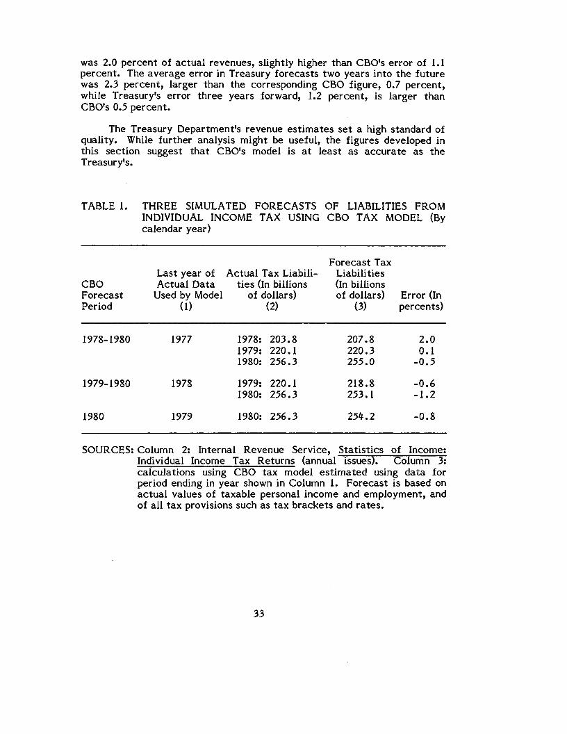
was 2.0 percent of actual revenues, slightly higher than CBO's error of 1.1percent. The average error in Treasury forecasts two years into the futurewas 2.3 percent, larger than the corresponding CBO figure, 0.7 percent,while Treasury's error three years forward, 1.2 percent, is larger thanCBO's 0.5 percent.

The Treasury Department's revenue estimates set a high standard ofquality. While further analysis might be useful, the figures developed inthis section suggest that CBO's model is at least as accurate as theTreasury's.

TABLE 1. THREE SIMULATED FORECASTS OF LIABILITIES FROMINDIVIDUAL INCOME TAX USING CBO TAX MODEL (Bycalendar year)

Last year of Actual Tax Liabili-CBOForecastPeriod

1978-1980

1979-1980

Actual DataUsed by Model

(1)

1977

1978

ties (In billionsof dollars)

(2)

1978: 203.81979: 220.11980: 256.3

1979: 220.11980: 256.3

Forecast TaxLiabilities(In billionsof dollars)

(3)

207.8220.3255.0

218.8253.1

Error (Inpercents)

2.00.1

-0.5

-0.6-1.2

1980 1979 1980: 256.3 254.2 -0.8

SOURCES: Column 2: Internal Revenue Service, Statistics of Income;Individual Income Tax Returns (annual issues). Column 3:calculations using CBO tax model estimated using data forperiod ending in year shown in Column 1. Forecast is based onactual values of taxable personal income and employment, andof all tax provisions such as tax brackets and rates.

33

TABLE 2. ANALYSIS OF ERRORS IN TREASURY DEPARTMENT FORECASTS OFINDIVIDUAL INCOME TAX REVENUES FOR FISCAL YEARS 1977-1981

Memorandum

YearIn WhichForecastWas Made

1977

1978

1979

1980

1981

SOURCES:

ActualRevenues(In billionsof dollars)

(1)

1978 181.01979 217.81980 244.1

1979 217.81980 244.11981 285.9

1980 244.11981 285.91982 297.7

1981 285.91982 297.7

1982 297.7

Columns (1) and (2):

ForecastedRevenues(In billionsof dollars)

(2)

171.2205.3234.1

190.1223.9262.9

227.3269.1311.2

274.4318.7

331.7

The Budget

Error(In

percents)(3)

5.45.74.1

12.78.37.9

6.95.8

-4.5

3.9-7.1

-11.4

TechnicalError

(Inpercents)

(4)

-1.12.9

-0.5

1.9-0.1-1.4

0.3-1.41.7

-1.84.6

5.1

of the United States

Errorfrom

InaccurateEconomicForecast

(Percents)(5)

4.25.55.9

4.54.56.2

5.77.83.9

6.3-1.2

-7.7

Errorfrom

InaccurateLegislative

Assumptions(Percents)

(6)

2.3-2.7-1.3

6.33.83.1

0.9-0.7

-10.1

-0.5-10.5

-8.9

Government, issues forvarious fiscal years. Columns (4)-(6): calculations described in the appendix.

34

CHAPTER IV. ISSUES IN INDIVIDUAL INCOME TAX REVENUES

The effects of inflation on federal revenues have recently focusedattention on several important questions. What has been the revenueimpact of the recent slowdown in inflation? How will revenues—and thedeficit—behave when indexation of the individual income tax takes effectin 1985 as currently scheduled? This chapter discusses these and otherproblems using estimates from the CBO individual income tax model.

THE RESPONSE OF TAX LIABILITIES TO INCREASESIN INCOME CAUSED BY INFLATION

With an unindexed individual income tax, inflation causes revenues toincrease relatively fast because of bracket creep. Increases in aggregatenominal income from inflation result in proportionally larger increases inincome tax liabilities than those reflecting real economic growth.

This difference in tax response arises from variations in the patternby which different changes in income are distributed. Increases reflectinginflation accrue primarily to existing taxpayers and are added to theseindividuals1 previous incomes. Because the personal exemption and (in thecases of many taxpayers) the fixed zero bracket amount have already beenapplied to existing income, they are no longer available to protectinflation-induced increases in income. In addition, such increases are likelyto be taxed at higher rates than previous income because they fall intohigher brackets. In contrast, when aggregate income expands because ofreal GNP growth, some of the increase generally accrues to existing tax-payers through increases in productivity, but some of it also accrues to newtaxpayers. This is because increases in real output generally increaseemployment, and many of these new workers are also new taxpayers. Theirincomes are relatively well-protected by deductions and exemptions, andare taxed at relatively low rates.

The differences in the response of tax liabilities to different changesin aggregate income are illustrated in the top panel of Figure 4. Thisfigure shows estimates from the CBO individual income tax model of theelasticity of the unindexed tax with respect to income for differentcombinations of real growth and inflation. This "income elasticity" isdefined as the ratio of the percentage change in tax liabilities occurringbecause of a change in income to the percentage by which income changes.The calculations are based on the assumption that all tax rate reductions

35

Figure 4.Implicit Elasticity of Tax Liabilities with Respect to Taxable PersonalIncome Under Indexed and Unindexed Taxes, Assuming DifferentRatios of Growth in the GNP Deflator to Total Nominal GNP Growth.Elasticity

1.7

Unindexed Tax

1.6

1.5

1.4

1.3

1.2

1.1

1.0 h

I Io.o

Elasticity

1.7

1.6

1.5

1.4

1.3

1.2

1.1

1.0

00.0

0.2

0.2

0.4 0.6 0.8Ratio

Indexed Tax

0.4 0.6 0.8

1.0

1.0Ratio

36

mandated by the Economic Recovery Tax Act of 1981 (ERTA) have takeneffect, but not the indexing provisions. Different points on the graph,moving from left to right, represent different degrees to which the growthof nominal GNP is assumed to represent real economic growth as opposedto inflation. For example, at the extreme lefthand side of the graph, GNPgrowth is assumed to be entirely "real"; halfway from left to right, thenominal GNP growth rate is assumed to reflect real and inflationarygrowth in equal proportions; and so on.

The difference between the elasticity value shown in Figure 4 and 1.0shows how much faster tax revenues grow than income. For example, thefigures for increases in GNP that primarily reflect inflation (at the right-hand side of the graph) approach values of 1.7; this suggests that, underthose economic conditions, individual income tax revenues may grow nearly70 percent faster than income. At the other extreme, when increases inGNP stem entirely from real economic growth, the elasticity is 1.3,suggesting that income tax liabilities grow more slowly—30 percent fasterthan GNP.l

These measures of elasticity show more variability than those pre-sented in most other sources (see those cited in footnote 2 of ChapterI.) This is because this study, unlike others, takes into account thefact that changes in the business cycle affect the distribution oftaxable income and, with it, the behavior of the tax. The generalproposition that income distribution changes over the cycle has beendemonstrated in several previous studies (cited in footnote 4 ofChapter 2), but only one other study has taken the tax implicationsinto account. See Frank deLeeuw, Thomas H. Holloway, DarwinJohnson, David S. McClain, and Charles A. Waite, "The High-Employ-ment Budget: New Estimates, 1955-80," Survey of Current Business(November 1981).

The estimates in Figure 4 were computed as follows. Using a currentCBO projection of economic conditions in 1985 as a basis, andassuming that nominal GNP grows at 8 percent between 1985 and1986, each of the different hypothetical combinations of growth ratesfor real GNP and the GNP deflator was analyzed in turn. On the basisof each, it was possible to predict consistent levels of aggregateemployment and taxable personal income using separate econometricequations. These predicted levels were used in the full tax model togenerate corresponding predictions of 1986 tax liabilities. The implic-it elasticity of tax liabilities with respect to income was given in eachcase by the ratio of the predicted percentage growth in tax liabilitiesto predicted percentage growth in taxable personal income. Thecalculations are described in detail in Congressional Budget Office,

37

It is important to realize that it is only the individual income taxamong federal revenue sources that exhibits these relatively high levels of(and variations in) responsiveness to changes in income. This tax accountsfor about half of federal revenues. Other important revenue sources,principally the social insurance payroll taxes and, to a lesser extent, thecorporate income tax, respond less strongly to changes in income. Theirresponsiveness, moreover, varies less with changes in the composition ofincome.

REVENUE IMPLICATIONS OF THE RECENT SLOWDOWN IN INFLATION

Because individual income tax revenues under the unindexed tax areso sensitive to inflation, the unexpectedly sharp slowdown in inflation thattook place during 1981 and 1982 has been singled out in some analyses as amajor factor in increasing the budget deficit. Slower-than-expected priceincreases, it is argued, have reduced the rate of bracket creep and theassociated growth in revenues, leading to bigger-than-expected deficits.2

The importance of this factor in the recent growth of the federaldeficit can be investigated using the CBO income tax model. Table 3shows CBO's projection of inflation for 1982-1986 as of midyear 1981 andearly 1983. As the figures show, inflation actually experienced in 1982 wassignificantly less than projected. As a result, the early 1983 projection offuture price growth was revised downward. The revenue implications ofthis revision can be isolated by comparing estimates of revenues generatedby bracket creep based on the two different inflation forecasts.3

The results are shown in Table 3. The inflation rate, as measured bythe CPI, was over two percentage points lower during 1982 than had beenforecast in early 1981. Similarly, CBO's more recent forecast of inflationduring the 1983-1986 period is below the 1981 forecast for the same periodby more than two full percentage points over the four years. Thesereductions in inflation alone—apart from all other unforeseen economic and

Footnote ContinuedSimulated Individual Income Tax Elasticities, unpublished technicalpaper (1983).

2 See, for example, Budget of the United States Government, FiscalYear 1984, pp. 3-19.

3 Using each inflation forecast, revenues were estimated by calculatingthe difference between the income tax revenues that would becollected in the absence of the Economic Recovery Tax Act, and thosethat would be collected if the income tax were indexed for inflation.

38

TABLE 3. CHANGE IN PREDICTED INDIVIDUAL INCOME TAX REVE-NUES FROM REVISION IN CBO INFLATION FORECAST FOR1983-1986

Forecast 1982 1983 198* 1985 1986

CBO Forecast of Rate ofIncrease in ConsumerPrice Index (Calendaryears, in percents)a

September 1981 8.3 6.2 5.5 4.7 4.2February 1983 6.2b 4.5 5.0 4.7 4.1Change, 1981 to 1983 -2.1 -1.7 -0.5 — -0.1

Estimated Reductionin Individual IncomeTax Revenues (Fiscalyears, in billionsof dollars) 20 24 35 42 52

SOURCE: Congressional Budget Office.

a. Year over year.b. Actual.

legislative developments—are estimated to reduce individual income taxrevenues by $24 billion in fiscal 1983, and successively greater amounts inlater years. This item represents 17 percent of the amount by which CBO'sbaseline deficit forecast for fiscal 1983 increased between mid-1981 andearly 1983. The remainder of the increase was a consequence of the factthat the economy was weaker during 1982 than had been predicted earlier,and of the changes in tax and spending policy that were not assumed in the1981 projections.

THE REVENUE IMPACT OF TAX INDEXATION IN 1985

ERTA includes provisions to protect taxpayers from bracket creep byindexing various tax provisions to the Consumer Price Index for All UrbanConsumers (CPI-U) beginning January 1, 1985. The personal exemption,zero bracket amount, and all other bracket boundaries will be adjustedeach year by the percentage by which the CPI-U has increased during the

39

preceding fiscal year.^ These provisions are designed to protect taxpayersfrom increases in effective individual income tax rates caused by inflation.Without indexation, inflation reduces the effectiveness of exemptions andthe zero bracket amount in shielding income from the tax, and pushesincomes into higher and higher brackets. This will no longer occur underindexation. *

For federal budget trends, indexation implies that, for the first time,increases in individual income tax revenue may react more strongly to realeconomic growth than inflation. This shift will take place because anybracket creep under the indexed tax will result from increases in produc-tivity rather than inflation. Income increases from this source would notbe prevented from moving individuals into higher tax rate brackets bycompensating changes in tax provisions under indexation.

The degree of importance of this productivity-induced bracket creepin quantitative terms can be investigated using the CBO income tax model.The bottom panel of Figure 4 shows model estimates of the incomeelasticity of aggregate income tax liabilities under the indexed tax. Likethe data for the unindexed tax shown in the top panel, these estimates aregiven for different combinations of inflation and real economic growth.6

The formal provision calls for adjustment on January 1 of each year bythe proportion by which the CPI-U grew on average during thepreceding fiscal year relative to its average level during fiscal year1983.

The accuracy of this generalization is affected by certain complica-tions regarding the indexing scheme. The tax provisions are indexedwith respect to consumer prices rather than wages or other measuresof incomes. As a result, in periods when consumer prices rise fasterthan incomes, taxpayers will be overprotected by indexation: theirreal tax burden may fall as a percentage of their incomes sinceindexed tax provisions will rise faster than incomes. In periods inwhich wages rise faster than consumer prices, on the other hand, thereverse will occur, and real tax rates may rise slightly. Even if wagesand consumer prices change at the same rate, real tax burdens mayfluctuate because incomes are determined by current inflation whilethe tax provisions are indexed with respect to inflation that occurredseveral months previously. If inflation increases from year to year,real tax burdens will rise, while if inflation falls, tax rates will falltoo.

These data were computed as described in footnote 1 of this chapter,but with one additional provision. To take account of indexation, the

Figure 4- shows that, when aggregate income growth is entirely due toinflation, indexation protects taxpayers in the aggregate from any increasein their tax rate—any bracket creep, that is; revenues rise only as fast asreal income does. When income increases are assumed to be entirely dueto real economic growth, and to reflect productivity growth to the extentthat they generally have in the past, however, some bracket creep willoccur. As a result, income tax revenues will grow about 30 percent fasterthan income. This is substantially less than the proportion by which taxgrowth outruns income growth under the unindexed tax.

ECONOMIC IMPLICATIONS OF INDEXATION

Taxpayers will approve of the effects of indexation in eliminating thesignificant "unlegislated tax increases" that are caused by inflation andbracket creep under the unindexed tax. Certain gains in economicefficiency, too, may result over time from the introduction of indexation,since it will prevent marginal tax rates from drifting upward.

On the other hand, indexation could also have some adverse effectsfrom the point of view of economic policy. The significantly slower growthin federal revenues that it implies will contribute to the tendency offederal budget deficits to increase over time (in the absence of legislationto control them). The persistent expectation of large and rising deficits,in turn, may be one explanation for the persistently high levels of interestrates, which threaten long-run productivity growth by reducing investment.Indexation may also reduce the automatic stabilization that the unindexed

Footnote Continuedpersonal exemption and zero bracket amount in Part I of the modeland all bracket boundaries in Part II were increased in each simulationby the percentage by which the GNP deflator was assumed to increase.

This procedure necessarily abstracts from the way the indexed tax willwork in practice. As has already been pointed out, the tax is actuallytied to lagged changes in the CPI, not to contemporaneous changes inthe GNP deflator, as was assumed in the sumulations. The simplerassumptions underlying these calculations were chosen because nosatisfactory quantitative generalizations are possible regarding differ-ences between current and lagged inflation or between inflation re-flected in the CPI and that reflected in the GNP deflator. The actualindexed tax will behave as is shown in the simulations to the extentthat inflation does not change from one year to the next and to theextent of differences between the CPI and the GNP deflator.

tax contributes to the economy under some circumstances by automaticallyreducing incomes and spending when they grow too fast and becomeinflationary in themselves. Overall, then, the significant changes in thebehavior of the income tax that are reflected in the estimates in thischapter have both positive and negative implications for the performanceof the economy.

APPENDIX

APPENDIX. ANALYSIS OF ERRORS IN TREASURY REVENUEFORECASTS

This appendix explains the calculations underlying the analysis shownin Table 2 in Chapter III of errors in Treasury forecasts of individualincome tax revenues. The discussion deals explicitly only with the errors inthe forecast made in 1977 (the first three lines of the table). Theprocedure underlying the remaining entries in the table is identical.

All data, except actual values of personal income, are drawn fromissues of The Budget of the United States Government for various fiscalyears. This document will hereafter be called the "Budget." The followingdata were required to analyze the 1977 Treasury forecast (all dollaramounts are in billions; all years are fiscal unless otherwise noted):

1. Forecast individual income tax revenues (from the 1978 Budget,p. 46); see Table 2, column 2.

2. Actual individual income tax revenues (from the Budgets for1980 (p. 61), 1981 (p. 61), and 1982 (p. 65)); see Table 2,column 1.

3. Estimated revenue impact of proposed legislation (from the 1978Budget, p. 46):

a. 1978: -19.2b. 1979: -22.5c. 1980: -31.8 .

4. Estimated revenue impact of enacted legislation

a. 1978: -15.3 (1979 Budget, p. 51)b. 1979: -18.5 (1979 Budget, p. 51)c. plus: -10.2 (1980 Budget, p. 67)d. 1980: -18.4 (1979 Budget, p. 51)e. plus: -16.9 (1980 Budget, p. 67) .

5. Forecast of personal income on which initial revenue forecastwas based (by calendar years):

a. 1978: 1,684 (1978 Budget, pp. 41-42)b. 1979: 1,879 (1978 Budget, pp. 41-42)

45

c. 1980: 2,075 (1978 Budget, pp. 41-42) .

6. Forecasts of personal income on which estimates of revenueimpacts of enacted legislation were based (by calendar years):

a. 1978: 1,704 (1979 Budget, pp. 31-33)b. 1979: 1,892 (1979 Budget, pp. 31-33)c. 1980: 2,095 (1979 Budget, pp. 31-33)d. 1978: 1,707 (1980 Budget, pp. 35-36)e. 1979: 1,894 (1980 Budget, pp. 35-36)f. 1980: 2,078 (1980 Budget, pp. 35-36) .

7. Actual personal income (by calendar years; from National In-come and Product Accounts, 1983):

a. 1978: 1,733b. 1979: 1,951c. 1980: 2,160 .

The first computation was made for the error introduced into eachrevenue forecast by an inaccurate assumption about the level of personalincome in the year being forecast. The appropriate adjustment involvedmultiplying actual revenues for a given year (item 2) by the ratio ofassumed personal income (item 5) to actual personal income (item 7) afterthis ratio is raised to the power of the elasticity of tax revenues withrespect to income. This elasticity was assumed to be 1.5. The result ofthis calculation was subtracted from actual revenues (item 2). Expressedas a percentage of actual revenues in each year, this difference appears incolumn (5) of Table 2.

The second computation was the error in each year's revenue forecastthat was caused by inaccurate assumptions about the tax provisions thatwould be in effect in a given year. This was taken to be the difference inthe Treasury's assumption regarding the revenue impact of tax legislationthat the Administration was proposing at the time the revenue forecastwas made (item 3) and its later estimate of the revenue impact of taxlegislation that had actually been enacted (item 4). Before item 4 wassubtracted from item 3, item 4 was adjusted for differences in the level ofpersonal income that was assumed for a given year in estimating item 4from the level that had been assumed for the same year in estimating item3. A revenue impact estimate based on one income assumption can beadjusted to another assumption by multiplying it by the ratio of the twoincome levels raised to the power of the income elasticity of tax receipts,which was assumed here to be 1.5.

46

Before being subtracted from item 3a, for example, item 4a wasmultiplied by the ratio of item 5a to item 6a raised to the power 1.5.Similarly, the legislation adjustment for the 1979 revenue forecast wascarried out by multipying item 4b by the ratio of 5b to 6b raised to 1.5,multiplying *c by the ratio of 5b to 6e raised to 1.5, adding these twoproducts together, and subtracting the result from 3b. The result ofsubtracting adjusted figures in item 4 from the corresponding element ofitem 3, taken as a percentage of actual revenues in the given year, is theestimated error introduced by inaccurate legislative assumptions. It isshown as a percent of actual revenues in column (6) of Table 2.

The estimated technical error is the residual—the component of thetotal error in each year's revenue forecast (column (1) in Table 2 minuscolumn (2)) that remains after subtracting the errors due to inaccurateassumptions regarding personal income and tax legislation. It is shown,expressed as a percentage of actual revenues, in column (4) of Table 2.

o