In te g e r L in e a r P ro g ra m m in ghome.deib.polimi.it/malucell/didattica/appunti/4ENG.pdf ·...

I n t e g e r L in e a r P r o g r a m m in g

Federico Malucelli Appunti di introduzione alla Ricerca Operativa

2

1. Discrete linear optimization problemsAt the beginning of the course we formulated several problems, some of which implied the use oflogical variables (with values 0 or 1) or of integer variables. If the objective function and theconstraints are linear, this class of problems is known as discrete linear optimization.Let us consider an Integer Linear Programming (ILP) problem of the following type:

min cxAx! bx "Zn

+

where Zn+ denotes the set of dimensional vectors n having integer non-negative components. Figure 1

shows the geometric representation of such a problem, where the feasible region is given by the onlypoints falling on the crossings of the squared area.

c

Fig. 1: the points of the feasible region are marked in red

Note that the feasible region (consisting of a discrete set of points) is not a convex set anymore, as itwas the case in linear programming. Consequently, the theory we developed for LP, as well as therelevant algorithms we examined, cannot be directly applied to this class of problems.

In addition to integer linear programming problems, the discrete linear optimization class of problemsalso includes Mixed Linear Programming problems (MLP), that is the LP class of problems in whichonly one subset of variables has integer values. Here is an example of MLP problem:

min cx + dyAx +Dy ! b

x"Zn+, y "Rn

A particular case of integer linear programming is represented by Combinatorial Optimization (CO),that is the class of problems in which the feasible region is a subset of the vertices of the unithypercube F # Bn= {0,1}n, i.e., more simply, problems in which variables can only take value 0 or 1.Linear {0,1} (or binary) programming problems, such as the one exemplified below, belong to thisclass.

min cxAx ! b

x "Bn


3

In the previous chapters we saw various CO problems, such as the knapsack problem, the travelingsalesperson problem and the spanning tree problem.Discrete optimization problems are generally difficult to solve. Yet, they represent a very importantclass of problems because they provide a very effective tool for the modeling of real problems, as wepreviously saw and as this chapter will show as well.To round off what already explained in Chapter 1, here we will examine a few formulations of discreteoptimization problems.Example: disjunctive constraintsSo far we have seen examples of problems in which the feasible region is described by a convexpolyhedron. But in some cases this property might be missing and the feasible region might be givenby a non-convex polyhedron. Let us consider, for example, the feasible region described in Figure 2.

1

1 x1

2x

Fig. 2: example of non-convex feasible region

As illustrated in Figure 3, the region can be described as a union of the two convex polyhedra P andQ.

1

1 x1

2x

1

1 x1

2x

P

Q

Fig. 3: decomposition of the polyhedron

The polyhedron P is given by P={x"R2: x1 - x2 $ 0, x2$1, x1!0, x2!0}, whereas Q={x"R2: x1 + x2 $1, x1!0, x2!0}. We know that, in order to find the intersection of the two polyhedra, it suffices that allconstraints of P and Q hold at the same time; otherwise, if we are seeking the union, we have to imposethat at least one of the two groups of constraints holds. First of all, we observe that some constraintsare common to the two polyhedra, in particular {x2$1, x1!0, x2!0}, so we can actually perform theintersection of these constraints, whereas the constraints more specifically characterizing the twofeasible regions are x1 - x2 $ 0 as regards P and x1 + x2 $ 1 as regards Q. We have to take care that inour formulation at least one of these two constraints holds; considering the problem from the oppositepoint of view, this means that at most one of these two constraints can be made redundant. Asillustrated in Figure 4, canceling one of these constraints means translating it by a quantity sufficient tomake it include the whole feasible region of the other polyhedron.


4

1

1 x1

2x

1

1 x1

2x

P

Q

x1 + $ 22x

x1 - $ 12x

Fig. 4: translation of constraints

In order to perform the operation of canceling at most one constraint (or one group of constraints) ofthe two that had been found, we introduce the variables 0-1 yP and yQ having value 1 if we decide tocancel the constraint relative to P or to Q, respectively. Hence, the formulation of the region shown inFigure 2 becomes:

x2$1x1!0x2!0x1 - x2 $ 0 + MPyPx1 + x2 $ 1 + MQyQyP + yQ $ 1yP, yQ " {0,1}

The constraint yP + yQ $ 1 allows to cancel at most one of the two groups of constraints. The choiceof the two constants MP and MQ has to be such as to guarantee that the feasible region is completelycontained inside the translated constraint. Therefore, in the examined case we have MP ! 1 and MQ !-1.

A particular case in the application of the technique of disjunctive constraints concerns machine taskscheduling problems. Let us pose the problem of processing n tasks 1,…,n on m machines denoted by1,…, m. Each task must be first performed on machine 1, then on machine 2, and so on up to the lastmachine m. The execution time of task j on machine k is given by sjk, j=1,…,n and k=1,…,m. Thedifferent machines can perform one task at a time, and the tasks performed by each machine must bebrought to an end, i.e., they cannot be interrupted and resumed. The problem consists in determiningthe sequencing of the different tasks on the different machines, trying to minimize the end time of thelast task (in technical language called makespan). To determine the sequencing we need variables tjkthat set the beginning time of task j on machine k. These variables make it easy to formulate theconstraints relative to the making sequence of each task:

tjk + sjk $ tjk+1 j=1,…,n, k=1,…,m-1Task j cannot start to be performed on machine k+1 before having been completed by machine k. Inorder to properly represent the objective function, which is of the bottleneck type (min max), weintroduce a variable T that will be greater than or equal to the end time of the last task on the lastmachine:

tjm + sjm $ T j=1,…,nObviously, the objective function will tend to minimize T, so that in the optimal solution T willprecisely take the end time of the last task:


5

min T

Now we just have to formulate the constraints preventing to perform two tasks on the same machinesimultaneously. This idea of non-simultaneity is expressed by considering each pair of tasks i and jand each machine k, and by imposing that on machine k either i precedes j or j precedes i, that is:

tik + sik $ tjkor

tjk + sjk $ tikTo express the disjunction between the two constraints we need a variable 0-1 yijk having value 1 if iprecedes j on k and 0 otherwise. The (disjunctive) constraints are:

tik + sik $ tjk + M(1-yijk) i, j=1,…,n, (i%j), k=1,…,mtjk + sjk $ tik + Myijk i, j=1,…,n, (i%j), k=1,…,m

where M is a value being high enough.

If we generalize the technique of disjunctive constraints that we saw for the non-convex region caseand for the scheduling problem, we can now consider the problem of determining a solution satisfyingat least k (1$k$n) of the constraints:

Aix $ bi, i = 1,…,n.

Let M"R: Aix –bi $ M, for each feasible x, i = 1,…,n.The problem can be formulated as follows:

Aix $ bi + Myi, i = 1,…,n,

&i=1

n yi $ n - k,

y " {0,1}n.

ExerciseFormulate the following problem as ILP: min {cx: x "X }, where the feasible region X is indicated in Figure 5.

x

x

1

21

3

Fig. 5

Example: piecewise linear functionsBefore Italian telephony was deregulated, the rates for private subscribers were the following: for thefirst 140 units the cost was 50 liras, from the 141th to the 220th unit the cost was 207 liras and for thefollowing units it was 127 liras. Figure 6 shows a scheme of such cost function, where b0 represents afixed cost (for example the bimonthly fee).


6

140 220 units

b0

cost

Fig. 6: old Sip rates for private subscribers

Hence, if x indicates the number of units and f(x) the cost function, we formally have:

f(x) =

'()(*

0 if x = 0

b0 + 50x if 0 < x $ 140

b1 + 207x if 140 < x $ 220

b2 + 127x if 220 < xwhere b1 and b2 are the values of the intercept of the red and the green lines represented in the figure.If we want to use this cost function in an optimization problem, we have to face the difficulty of anobjective function which is not linear but piecewise linear. A way of dealing with these functions is touse integer linear programming models. The idea is to deal with the three intervals [0,140], [140,220],[220,M] separately, with M being an appropriately large constant. Let us introduce the continuousvariables z0, z1 and z2 indicating how many units are spent in the first, in the second and in the thirdband, respectively. We also have to introduce a mechanism preventing to spend the units of an intervalif the units of the preceding interval have not already been used up. This is done by introducingvariables 0-1, one for each interval, (y0, y1 and y2) having value 1 only if we have started to spend someunits in the interval they refer to. The objective function and the constraints that operate the mechanismwe mentioned are the following:

min b0y0 + 50z0 + 207z1 + 127z2140 y1 $ z0 $ 140 y080 y2 $ z1 $ 80 y10 $ z2 $ M y2x = z0 + z1 + z2y0, y1 and y2 "{0,1}

Note that if, for example, z1>0 then y1 must be equal to 1, which implies that z0 must be equal to 140,thus we must have used up all the units of the preceding interval.Wishing to apply what we saw for the telephone rate example to a more general context, we have toconsider the following piecewise linear function to be minimized, whose graphical representation isshown in Figure 7:

f(x)=

'(()((*

0, if x =a0,b0 + c0(x - a0), if a0 < x $ a1,b0 + c0(a1 - a0) +b1 + c1(x-a1), if a1 < x $ a2,… …

&i=1

k-1 [bi-1 + ci-1(ai - ai -1)] + bk-1 + ck-1(x-ak-1), if ak-1 < x $ ak.


7

0b

1b

k–1b

c0

c1

ck - 1

aka2 ak - 1a1a 0 x

f(x )

Fig. 7: general piecewise linear functionProblem P can be formulated as an ILP problem as follows:

(P') min &i=0

k-1 bi yi + ci zi

(a1 - a0)y1 $ z0 $ (a1 - a0)y0,(a2 - a1)y2 $ z1 $ (a2 - a1)y1, … … …

0 $ zk-1 $ (ak - ak-1)yk-1,

x = &i=0

k-1 zi + a0,

yi "{0,1}, zi "R, i = 0,…, k-1.

Let ( y _

, z _

, x _

) be a feasible solution for P'. We want to show that it gives

f( x _

) = &i=0

k-1 bi y

_i + ci z

_i.

Consider y _

. Assume that it gives y _

r-1= 1, y _

r = 0, 1$ r $ k-1.

y _

r = 0 + '(()((* y _

i = 0, i ! r,

z _

i = 0 i ! r;

y _

r-1 = 1 +

'(()((* y

_i = 1, i $ r -1,

z _

i-1 = ai - ai-1 i $ r -1,

0$ z _

i-1$ ai - ai-1, i = r;

Hence:


8

&i=0

k-1 bi y

_i + ci z

_i = &

i=0

r-1 bi + &

i=1

r-1 ci-1(ai - ai-1) + cr- 1 z

_r-1

= &i=0

r-1 bi + &

i=1

r-1 ci-1(ai - ai-1) + cr- 1( x

_ - ar-1).

The last equality derives from the fact that, according to construction, we have:

x _

= ar-1 + z _

r-1 with 0 $ z _

r-1$ (ar - ar-1),

hence f( x _

) = &i=0

k-1 b i y

_i + ci z

_i.

In some particular cases it is not necessary to introduce variables 0,1 in order to induce the sequencingmechanism in the growth of variables z. One of these cases is, for instance, the minimization of aconvex piecewise linear function, as exemplified in Figure 8.

x

f(x)

Fig. 8: convex piecewise linear function

With such function we can intuitively understand that it is more advantageous to use the initial part ofthe function, with lower unit costs, before moving on to the following parts. Clearly, such functionscan be formally represented using the technique of bottleneck objective functions that we saw in thefirst chapter. Let there be the convex piecewise linear function:

f(x) =

'()(*

b0 + c0x if 0 $ x $ a0

b1 + c1x if a0< x $ a1

… …

bn + cnx if an-1< xIf we consider the different lines, including those outside the interval definition field, we see that thefunction is always given by the higher line, therefore:

f(x) = max{bi + cix, i=0,…n-1}.

ExerciseConsider a concave piecewise linear objective function f(x). Formulate the problem of maximizing f(x) in terms oflinear programming.

Example: the traveling salesperson problem on a directed graphConsider the traveling salesperson problem, i.e., the problem of determining a minimum costHamiltonian cycle on a weighted symmetric graph G=(N,A,c) where |N| =n. In Chapter 2 we saw apossible formulation of the traveling salesperson problem on undirected graphs; let us now examinethe directed case.


9

Let x = [xij] be a vector of binary variables with the following meaning:

xij = ')*1, if arc (i,j) belongs to the Hamiltonian cycle we look for, 0,otherwise.

A first set of constraints says that exactly one arc must arrive at and leave from each node:

X1 = {x: &i=1

n xij = 1, &

j=1

n xij = 1, xij " {0,1}, i = 1,..., n, j = 1,..., n }.

Just like in the undirected case, we have to remove subcycles, i.e., cycles not traversing all the graphnodes. A possible way to do this is the following:

X2 = {x: &i"N1

&j"N2

xij ! 1, , (N1, N2,) : N = N1-N2, N1.N2=Ø, N1%Ø, N2%Ø},

Considering any partition of nodes into two non-empty subsets, the number of arcs in the solutionwith tail in the first subset and head in the second one must be greater than or equal to 1. An alternativeway is to introduce other (continuous) variables ui that determine the order according to which eachnode i is visited. Constraints are used to define the value of variables determining the order.

X3 = {x: ui - uj + nxij $ n-1 , ui " R, i = 1,..., n, j =2,…n, i % j }.

The set X3 merely includes cycles containing node 1. In fact, we consider a cycle composed of k $ n-1nodes and not containing node 1; by adding together the constraints ui - uj + nxij $ n-1 correspondingto the arcs of the cycle, we get the contradiction kn $ k (n-1). Observe that X3 does not include theconstraints ui - u1 + nxij $ n-1, ui " R, i = 1,..., n, hence it is satisfied by cycles containing node 1.Consequently, the set X1 . X3 defines the set of Hamiltonian cycles on G.We can see now that variables ui provide the search order in a feasible solution.If arc (i,j) belongs to the Hamiltonian cycle (xij = 1), the corresponding constraint in X3 becomes:

ui + 1 $ uj.

Observe that a vector u _

satisfying the preceding constraints is given by u _

1= 0 , u _

i =k, i%1, if i is thek+1-th node of the cycle starting from node 1.If arc (i,j) does not belong to the Hamiltonian cycle (xij = 0), the corresponding constraint in X3becomes:

ui - uj $ n-1,

which is always satisfied by u _

because u _

i $ n -1 and u _

j ! 0.The traveling salesperson problem can be defined in one of these two alternative ways:

TSP1: min { &i,j =1

n cijxij : x " X1 . X2};

TSP2: min { &i,j =1

n cijxij : x "X1 . X3}.

Observe that TSP1 is defined by O(2n) constraints, whereas TSP2 is defined by O(n2) constraints.Example: selection of subsetsMany problems having a practical importance are formulated as a selection of subsets belonging to aspecific family. For example, problems of staff shifts belong to this class of problems.Let there be:- a set I = {1, 2,…, n},


10

- a family F of m subsets of I : F = {J1, J2,…, Jm}, Jj # I , j = 1,…, m,- the cost cj of the subset Jj, j = 1,…, m.The purpose is to determine a minimum cost family D # F, while respecting the constraint that eachelement of I belongs to:i) at least one subset of D (cover problem);ii) exactly one subset of D (partitioning problem);iii) at most one subset of D (packing problem).For example, in the case of shifts of airline pilots the set I is given by the flights to be covered, whereaseach subset Jj is defined by the flights that can be performed by the same pilot during a working week,while respecting union rules as well as the compatibility of flights depending on simple timeconstraints and on the type of aircraft. Finally, cj is the salary that must be paid to the pilot for aspecific work shift. It is a partitioning problem (we have to assign a pilot to each flight) but, since itmay be quite difficult to reach a feasible solution, we can consider it as a cover problem, taking the riskto have more than one pilot on the same flight.If we formulate the above problems in terms of integer linear programming, the family F can berepresented by the matrix A = [aij ], i = 1,…, n, j = 1,…, m, where:

aij = '()(*1, if i "Jj,

0, otherwise.

If we indicate the subset choice variables by

xj = '()(*1, if the set Jj"D,

0, otherwise,

then:- the cover problem can be formulated as:

min cxAx! ex "{0,1}m

where e denotes the vector whose components are equal to 1;- the partitioning problem can be formulated as:

min cxAx= ex "{0,1}m;

- the packing problem can be formulated as:

min cxAx$ ex "{0,1}m.

Example: vehicle routingA classical optimization problem in the transportation sector is the Vehicle Routing Problem. Let therebe: a set of clients to be served {1,…,n}, each having a demand of good di, and a set of k vehicles that,for more simplicity, we assume to be homogeneous, i.e., all having equal capacity Q and all kept in thesame depot we indicate with 0. The distances between each pair of clients and between the depot andeach client (cij, i,j = 0,…,n) are known as well. The problem consists in delivering the goods to allclients minimizing the total distance covered by the vehicles and respecting their capacity constraints.To support the formulation, we can consider a complete graph with nodes corresponding to clients andto the depot. A feasible solution consists in a family of m (m$k) cycles having origin in 0 such that allclients belong to one cycle. We can decompose the decisions into two levels: at the first level weassign clients to vehicles. To do so we use assignment variables:


11

yih = '()(*1, if node i belongs to the route of vehicle h,

0, otherwise.

The constraints referring to these variables are:

&h=1

k yih = 1 i=1,…,n

that is, each client must belong to a route. We can also have a bound on the number of used vehiclesby imposing a constraint on the number of times node 0 is assigned to a route:

&h=1

k y1h $ m

Constraints on vehicle capacity can also be easily expressed by imposing that the sum of demands bythe clients assigned to the same vehicle does not exceed the maximum capacity, and we do so using theconstraints we saw for the knapsack problem:

&i=1

n di yih $ Q h=1,…,k

If now we want to measure the distance covered by each vehicle, we have to solve as many travelingsalesperson problems as the number of vehicles that are used. So, we introduce variables xh

ij in order todetermine the route of vehicle h:

xhij= '()(*1, if vehicle h goes from node i to node j,

0, otherwise, i, j = 0,…,n, h = 1,…,k.

The feasibility constraints in the route choice (an incoming arc and an outgoing arc for each node andsubcycle removal) are:

&j=1,j%i

n xh

ij = yih i = 0,…,n, h=1,…,k

&j=1,j%i

n xh

ji = yih i = 0,…,n, h=1,…,k

&i,j"S

xhij $ |S|-1 S#{1,…,n} |S|!2, h=1,…,k.

We can remove a group of variables and simplify the model by observing that

yih = &j=1,j%i

n xh

ij

The complete formulation of the vehicle routing problem becomes:


12

min &h=1

k &

i=1

n &j=1

n cijx

hij

&j=1

n xh

ij = &j=1

n xh

ji = yih i = 0,…,n, h=1,…,k

&h=1

k &

j=1

n xh

ij = 1 i = 1,…,n,

&i=1

n &

j=0

n dix

hji $ Q h=1,…,k.

xhij " {0,1}, i,j = 0,…,n,

Example: frequency assignmentIn a cellular telecommunication network the territory is served by various antennas, each covering aspecific cell. Cells overlap each other in order to ensure continuity of service to users while they move.A classical problem in this field is to assign frequencies to cells so as to prevent that interfering cells(for example those that overlap) use the same frequency. A purpose can be, for example, to minimizethe number of used frequencies.

Fig. 9: cellular system

The problem makes use of a representation on a graph. Let us build an undirected graph G= (N,A)where nodes correspond to the cells of the telecommunication network and between two nodes there isan arc {i,j} if the corresponding cells interfere.

1 2 3

4 5 6 7

8 9 10

Fig. 10: graph of interferences

Having k available frequencies, in order to formulate the problem we use variables assigning nodes tofrequencies:

xih = '()(*1, if node i is assigned the frequency h,

0, otherwise.

Further, we need a set of variables determining the actual use of frequencies.

yh = '()(*1, if the frequency h is assigned to some node,

0, otherwise.

The problem formulation is:


13

min &h=1

k yh

xih + xjh $ 1 ,{i,j}"Axih , yh , ,i"N, h=1,…,k.

This problem on graphs is known in the literature as coloring problem: the purpose is to color thenodes of a graph in such a way that adjacent nodes are differently colored, while minimizing thenumber of colors. A well-known case is the coloring of geographical maps.2. Choice of the formulation and "polyhedral" methods of solutionUnlike in continuous linear programming, in ILP the choice of the formulation has a strong influenceon the efficiency of the methods of solution, and often proves to be a decisive factor. Let us considerthe following example.

max x1 + 0.64 x250x1 + 31x2 $ 2503x1 - 2 x2 ! -4x1, x2 ! 0 integers.

In Figure 11 we indicate the feasible region provided by the integer points contained in the polyhedrondefined by the linear constraints.

c

x

x2

1

x

Fig. 11: feasible region and optimal solution of the continuous problem

In the figure we also indicated the solution x– of the linear programming problem obtained eliminatingintegrity constraints from variables. Such problem can be easily solved by using the methods we sawin the preceding chapter, thus giving x–=[ ]376/193

950/193 , with value 5.098. Since we have no integer

components, such solution cannot be considered as the solution to the original ILP problem because itis unfeasible. We could try to obtain a feasible solution, possibly an optimal one, by approximatingfractional values to integer values being closer to the values of the components of x–. In the examinedcase, if we look at the drawing we notice that such solution might be x'=[ ]2

4 . Note that generating

such point is not so easy in general, that is when the space of solutions has a dimension being muchgreater than two. Anyhow, the obtained solution is not only rather difficult to generate, but in somecases also proves to be very far from the optimal solution of the ILP problem. In the examined


14

example the integer optimal solution is x*=[ ]50 , as it can be easily verified by comparing the values of

the objective function.Yet, we should ask ourselves what would have happened if, instead of using the above formulation withtwo constraints, we had used the following one, whose geometric representation appears in Figure 12:

max x1 + 0.64 x2-x1 + x2 $ 2x1 + x2 $ 63x1 + 2 x2 $ 15x1, x2 ! 0 integers.

c

x

x2

1

Fig. 12: geometric representation of the alternative formulation

We immediately notice that, from the point of view of the feasible region, the two formulations areequivalent; in fact they comprise the same set of integer points. However, the second formulation hasall vertices corresponding with feasible solutions for the ILP problem. Remember that, if in a linearprogramming problem the finite optimum exists, then at least one vertex of the polyhedron is optimal;this implies that if we leave out the integrity constraints and solve the corresponding LP problem, thesolution we obtain is integer, therefore it is optimal for the original problem as well.

The considerations we developed in the preceding example clearly illustrate how important it is todetect a good formulation of the problem. Let S be the set of feasible solutions of a specific discreteoptimization problem; we can detect the smallest convex set comprising all points of S:Definition 2.1Given a finite set of points S, the convex envelope of S, denoted with conv(S), is the smallest convexpolyhedron containing all points of S.

Consider the problems:

P: min cx P': min cxAx = b x"conv({Ax=b, x"Zn})

x"Zn

We rather intuitively understand that each vertex of the convex envelope is a point of S, hence theoptimal solution of P', due to the linearity of the objective function, is optimal for P as well. Yet, we


15

still do not know how to solve problem P, whereas P' can be solved by means of algorithms for linearprogramming. In fact, if there exists an optimal finite solution and at least one vertex of the polyhedroncoincides with an optimal solution, then such vertex belongs to S. These observations might induce usto think that solving a discrete linear optimization problem or an ILP problem is easy: we obtain theformulation of the convex envelope in term of linear constraints and we apply the algorithm for solvingLP problems that we know to be efficient. The difficulty, however, hides in the formulation of theconvex envelope. In fact, in several problems, for example in the traveling salesperson problem, it isnot possible to provide the complete formulation for instances of any size, whereas in general suchformulation, even when it is possible to characterize it completely, requires an exponential number ofconstraints, thus making the method of solution extremely inefficient.*2.1 Unimodularity

There are cases in which the polyhedron P–

:{Ax = b, x ! 0}, from which we have removed the integrityconstraints, coincides with the convex envelope P'=conv({Ax=b, x"Zn}). This happens when each

vertex of P–

, and therefore each of its bases, has integer components, i.e., it possesses the integralityproperty. It could be extremely helpful to characterize these problems, which reveal to be particularlyeasy to manage. Let us introduce some definitions that are useful to achieve this aim.Definition 2.2A matrix with integer components m×n, A , is unimodular if for each non-singular square submatrix Dbeing of maximum rank we get:

det(D) = ± 1.

Definition 2.3A matrix with integer components m×n, A, is totally unimodular (TU) if each of its non-singularsquare matrices is unimodular.Theorem 2.4If A and b have integer component and A is unimodular, then all basic solutions of the problem

min cxAx = bx ! 0

have integer components.ProofIn fact, let us consider a basis B and let A*

B be the adjoint matrix of AB. We have

xB=A-1B b =

A*B

det(AB)b,

hence the basic solution has integer components. /

Corollary 2.5If A and b have integer components and A is totally unimodular, then the problems:

min cx min cx Ax ! b Ax $ b x ! 0 x ! 0

have all basic solutions with integer components.ProofThe demonstration immediately follows by observing that if A is TU then also [A,I ], [A,-I ] are TU./


16

The characterization of totally unimodular has been the object of deeper study. Here we relate asufficient unimodularity condition which does not only involve an elegant demonstration, but also hasdirect consequences on an extensive class of optimization problems, such as those on network flows.Theorem 2.6A matrix A with elements 0, ±1 is TU if the following conditions hold:a) each column contains at most two non-null elements;b) the indexes {1,…,m} of the rows of A can be partitioned into two sets I1, I2 such that:

- if a column has two elements with the same sign, the indexes of corresponding rows do notbelong to the same set;

- if a column has two elements with opposite signs, the indexes of corresponding rows belong tothe same set.

ProofLet C be a square submatrix of A of order h. The demonstration is performed by induction on index h.If h =1, then according to definition we have det(C) =0, ±1.Let 1<h $n. We have the following exhaustive cases:i) either C contains at least one null column, hence det(C) =0;ii) or C contains at least one column with only one non-null element; in such case, by developing the

determinant starting from one of these columns and by making use of the inductive hypothesis, wehave det(C) =0, ±1;

iii) or each column of C has exactly two elements different from zero; hence, for the j-th column itgives:

&i "I1

cij = &i "I2

cij;

in fact, elements of the j-th column having opposite signs belong to the same set and thereforesuppress each other in the sum, whereas equal elements belong to different sets. Consequently,there exists a linear combination of rows that provides the null vector:

&i "I1

Ci - &i "I2

Ci = 0.

Hence det(C) =0./

As a consequence of the theorem 2.6, the incidence matrix of a directed graph is TU and also theincidence matrix of a bipartite undirected graph is TU. Therefore, flow problems, shortest-pathproblems, maximum-flow problems, bipartite assignment and transportation problems have integerbasic solutions. Remember that we had informally examined this property when studying flowproblems on a network and solution algorithms. Observe that, in general, the matrix of an undirectedgraph is not TU. In fact, an undirected graph is not bipartite if it contains at least one odd cycle. Let Cbe the incidence matrix of an odd cycle. It can be immediately verified that det(C) = ±2.2.2 "Polyhedral" or cutting-plane methodsResuming the idea of referring to a LP case by formulating the problem in terms of convex envelope, itshould be noted that it is not necessary to describe the polyhedron of the convex envelope completely,we can rather concentrate on the neighborhood of the optimal solution. Polyhedral or cutting-planemethods do nothing but iteratively refine the polyhedron of the convex envelope where we think theoptimal solution is situated. Consider the following integer linear programming problem:

P: min cxAx $ b

x"Zn+

as well as the problem in which we leave out the integrity constraints:


17

P–: min cxAx $ b

x ! 0

P– is a linear programming problem that we suppose to admit finite optimal solution x–. If x– has allinteger components, then it coincides with the optimal solution of the integer problem P, otherwise wecan try to refine the formulation of P– by adding appropriate constraints.Definition 2.7A valid inequality is a constraint gx ! 0, such that:

gx $ 0, ,x "{x"Zn+: Ax $ b}

Definition 2.8A cutting plane is a valid inequality gx $ 0, such that:

gx– > 0.

Therefore, if we detect a cutting plane for problem P– and its fractional optimal solution x–, we can addsuch inequality to the formulation and iterate the procedure while progressively approaching theinteger optimal solution. The process is summarized by the following procedure:

Procedure cutting_plane_method:begin

optimal:= false;repeat

Solve(P–

,x–);if x– has all integer components then optimal:= true

else beginGenerate_cut (g, 0);Add_cut(P

–,g , 0 )

enduntil optimal

end.Fig. 13: cutting-plane method

Consequently, it is essential to find a method allowing to generate cutting planes that are as effective aspossible, i.e., near to the polyhedron of the convex envelope. Now let us describe a method (that weowe to Chvátal) useful to derive valid inequalities which, however, are not necessarily cutting planes forthe fractional solution.Consider the integer programming problem

(P) min{cx : x"F},

where F = {x: Ax $ b, x"Zn+}, with A being a matrix m×n having non-negative integer components, b

being a column vector having m integer components and d having non-negative integer components.Theorem 2.9Given a vector u=[ui]!0 i=1,…,m, each inequality gx $ 0 with

gj = 1&i=1

m uiAij2,

(2.1) 0 = 1&i=1

m uibi2,


18

is a valid inequality for P.ProofWe call F– = {x: Ax $ b, x"Rn

+} and we consider the constraint:

(2.2) &j=1

n (&

i=1

m uiAij)x j $ &

i=1

m uibi .

Since it was obtained as a non-negative linear combination (with multipliers ui) of the constraintsAx $ b, such constraint is satisfied by each x " F–, therefore also by each x"F.Now let us consider the constraint

(2.3) &j=1

n gjxj $ &

i=1

m uibi .

Because x ! 0, the examined constraint is less stringent in comparison with (2.2), since originalcoefficients were replaced with their lower integer part; hence it is satisfied by each x"F. Because forx"F the left-hand side of (2.3) takes an integer value, the result is that the constraint

&j=1

n gjxj $ 0

is satisfied by each x"F, hence it is a valid inequality for P. /

Example: application of Chvátal inequalitiesConsider the following problem:

min -x1 - x2 - x3x1 + x2 $ 1

x2 +x3$ 1+x1 + x3$ 1xi!0, xi"Z, i=1,…,3

This formulation corresponds to the problem of determining a maximum cardinality matching in acomplete graph with cardinality 3. The optimal solution of the problem is obviously one andcorresponds to the choice of any arc (x1 or x2 or x3 equal to 1). Otherwise, if we solve the linearprogramming problem that leaves out the integrity constraints, we obtain 3/2 with each variable beingset at value 1/2. If we take u1=u2=u3=1/2 as multipliers, then the Chvátal inequality is:

11/2 + 1/22x1 + 11/2 + 1/22x2 + 11/2 + 1/22x3 $ 11/2 + 1/2 + 1/22

that is

x1 + x2 + x3 $ 1.Adding the inequality to the problem and leaving out the integrity constraints we obtain the integeroptimal solution.Obviously, the generation of Chvátal valid inequalities can be iterated; in other words, we can add thevalid inequality to the set of constraints and from the latter we can form a new valid inequality and soforth.We will call this procedure Generate_Inequality. The fundamental achievement brought about byChvátal is that we need a finite number of calls of Generate_Inequality to obtain the inequalitiesnecessary to define conv(F ). For details about this important result, see []Unfortunately, the above mentioned result does not provide constructive tools, that is it gives noinformation about how to determine a valid inequality that proves to be a cut as well. In the early


19

Seventies, Gomory proposed a general method, apparently infallible, of generating cuts for any integerlinear programming problem starting from the fractional optimal solution of the problem in whichintegrity constraints were left out.Consider the problem P

min cxAx = bx ! 0x " Zn

and the problem P–

in which we leave out the integrity constraints

min cxAx = bx ! 0.

Let x– = 13334

25556x–B

x–N be an optimal basic solution of P

–, hence x–B, = A-1

B b and x–N = 0. Writing in full the

constraints of problem P–

and pointing out the components in the base and those outside the base, wehave:

ABxB + ANxN = btherefore, if we derive the expression of xB in full we have:

(2.4) xB = A-1B b - A-1

B AN xN .

We call b– = A-1B b and A

– = A-1

B AN. If x–B has all integer components, then solution x– is optimal also for

P. Otherwise, it will exist a component h such that x–h has a non-integer value; let t be the constraintcorresponding to component h in the system (2.4), i.e.:

(2.5) xh + &j"N

a–tjxj = b–t = x–h.

Observe that (2.5) is a linear combination of the problem constraints with multipliers given by the t-throw of matrix A-1

B , therefore it is a valid constraint for the problem. Consider now the cutting off ofcoefficients on the left: we can generate the following valid inequality:

(2.6) xh + &j"N

1a–tj2xj $ b–t

Since we are dealing with solutions having integer components, we can state that the left-hand side of(2.6) must be integer, hence we can reinforce the inequality in the following way:

(2.7) xh + &j"N

1a–tj2xj $ 1b–t 2.

Now we just have to check that (2.7) is a cut, i.e., that it is not satisfied by x–. Given that x–N = 0, (2.7) isreduced to:

x–h $ 1b–t 2

which is obviously violated since x–h = b–t .


20

Example: application of Gomory cuts (1)Consider the problem:

min -x1 - x2-3x1 + 12x2 + x3 = 306x1 - 3x2 + x4 = 8xi"Z+

The optimal solution of the continuous problem is x–B = [ ]62/2168/21 where B = {1,2} and A-1

B =

[ ]1/214/212/211/21 . By applying (2.5) to the two fractional components of the solution we have:

x1 + 121 x3 + 4

21 x4 = 6221

x2 + 221 x3 + 1

21 x4 = 6821

therefore, Gomory cuts become:

x1 $ 2, x2 $ 3.ExerciseConsidering x3 and x4 as slack variables, graphically represent the problem and Gomory's cuts which were derived fromthe example.

Example: application of Gomory cuts (2)Given the ILP problem

max -0.1x1 + x2-4x1 + 4x2 $ 30x1 + 2x2 $ 8xi"Z+ i=1,2

The optimal solution can be graphically determined and lies in the intersection of the two constraints:x1=3/2 and x2=11/4. In order to approach the problem with the method of Gomory cuts, we introduceslack variables so as to turn constraints into inequalities. The problem, transformed in this way andwith relaxed integrity constraints, is the following:

max -0.1x1 + x2-4x1 + 4x2 + x3 = 30x1 + 2x2 + x4= 8xi!0 i=1,,…,4

The base B is {1,2} whereas N={3,4}. The different matrices that are involved in the computations are:

AB = [ ]-4 41 2 , AN= [ ]1 0

0 1

A-1B = A-1

B AN= [ ]-1/6 1/31/12 1/3

The Chvátal-Gomory cut referring to the first fractional variable is:x1 + 1-1/62 x3 + 11/32 x4 $ 13/22

hencex1 - x3 $ 1

replacing x3 by the expression derived from the first equation of the constraint system:x3 = 5 + 4x1 - 4x2

we get-3 x1 + 4 x2 $ 6.


21

The Chvátal-Gomory cut referring to the second fractional variable is:x2 + 11/122 x3 + 11/32 x4 $ 111/42

hencex2 $ 2.

ExerciseGraphically represent the problem, the fractional solution and the obtained cuts. Derive the new solution after theintroduction of the cuts.

The techniques illustrated above are wholly general and can be applied to any integer linearprogramming problem. There are also methods examining the characteristics of the polyhedra of thedifferent problems more closely and generating ad hoc inequalities for specific cases. Let us take theexample of a knapsack problem:

max &i=1

n ci xi

&i=1

n ai xi $ b

x " {0,1}n

Detecting a subset of indexes C for which

&i"C

ai > b

we can state that all objects in C cannot be present at the same time in a feasible solution, hence theinequality

&i"C

xi $ |C| -1

is valid. In a similar and at times quite sophisticated way, it is possible to obtain valid inequalities formany other problems, such as the traveling salesperson problem, the vehicle routing problem, graphcoloring, etc.3. Implicit enumeration methodsInstead of using polyhedral methods, discrete optimization problems can be approached usingalgorithms of the enumerative type. The concept on which this class of algorithms is based is rathersimple: we have to systematically enumerate all feasible solutions of the problem, evaluate the objectivefunction and choose the best one. Just to give an example, let us consider the following instance of theknapsack problem:

max 4x1 + x2 + 3x3 + x45x1 + 4x2 + 3x3 + x4 $ 8

xi"{0,1}, i=1,…,4.

The set of solutions of this problem can be enumerated using the decision tree shown in Figure 14.Let us consider the problem's variables (objects to be put into the knapsack) one by one, and let us"open" a new ramification of the decision tree for each possible value that can be assigned to theexamined variable (object that are put into the knapsack or that are discarded). Each node of thedecision tree corresponds therefore to a subproblem in which some variables have values that are fixedin advance and can be established according to the route connecting the node to the root of the tree.For example, node D corresponds to the subproblem in which we set x1 = 0 e x2 = 1:

1+ max 3x3 + x43x3 + x4 $ 8 - 4xi"{0,1}, i=3, 4.


22

root

1 0 1x

1 0 1 0

1 0 1 0 1 0 1 0

1 0 1 0 0 1 0 1 0 1 0 1 0 1 01 x 4

2x

3x

A B

C D

Fig. 14: decision tree for a knapsack problem 0-1 with 4 objects

Nodes of tree level i are 2i because in the examined case the values we assign to each variable are 2.Paths from the root to the leaves detect the attributions of values {0,1} to variables and therefore alsosome solutions (not necessarily feasible) for the considered problem. For example, the path from rootto leaf A detects an unfeasible solution of the considered knapsack problem (the global weightamounts to 13 and the capacity is 8), whereas the path from root to leaf B detects a feasible solutionhaving value 7. Therefore, the aim is to detect among all the leaves corresponding to feasible solutionsthe one having the best value.Observe how the nodes of the decision tree increase exponentially with the problem size, thus analgorithm actually proceeding to the explicit enumeration of all nodes reveals to be not much efficient.Therefore, we have to use "tricks" allowing to remove useless portions of the tree, thus reducing thenumber of nodes to evaluate.A starting criterion should enable us to recognize as soon as possible when a subtree does not containany feasible solution. In the case of Figure 14, once arrived at node C we realize we have alreadyexceeded the knapsack's capacity and it is no use proceeding to the enumeration of the subtree havingroot C. In this way, entire subtrees can be discarded and considered as implicitly visited: then we speakof implicit enumeration algorithms. If we proceed to the reduction according to this criterion, what isleft is the tree shown in Figure 15.

root

1 0 1x

0 1 0

1 0 1 0 1 0

0 1 0 1 0 1 0 1 0 1 0 x4

2x

3x

Fig. 15: decision tree that has been reduced according to the feasibility criterion


23

A second criterion allowing to reduce the extent of the enumeration is related to the value of solutions.Suppose we have an available feasible solution with value v. For example, in the knapsack case wecould find a feasible solution by using the algorithm we saw in Chapter 1 (burglar problem): x3=x4=1,x1=0, x2=1, v=5. If, when developing the decision tree, we realize that a subtree does not containsolutions having value greater than 5, then it is no use to proceed to the enumeration of the subtree,even if it contains feasible solutions. The most critical point is how to estimate the best solution valueof a subtree without making use of the enumeration. In the examined example a very roughoverestimation of the best solution value could be the one that chooses the objects to be put into theknapsack while completely leaving out the capacity constraint. If the overestimation computed at a treenode is smaller than or equal to the value of the available solution, then we can avoid continuing theenumeration of the subtree. According to this criterion, the enumeration tree is further reduced, asshown in Figure 16. Beside each node we indicate the estimation value. Note that on the leaves theestimation coincides with the solution value.

root

1 0 1x

0

1 0

0 x4

2x

3x

9

9

8

5

8 5

7Fig. 16: decision tree reduced according to the criterion of overestimation of the optimal solution

The example developed above provides the main ideas of an implicit enumeration algorithm, which isknown as Branch&Bound and can be summarized in the few following code lines: the procedure takesas input a problem P in maximization form as well as the value of a feasible solution v.

Procedure Branch_and_Bound(P,v);begin

b=Bound(P,x,unfeasible);if x is integer then return (b);else if unfeasible return(-7);

else if b>v thenbegin

Branch(P,x,P1,P2,…,Pk)for i=1,…,k do begin

t:= Branch_and_Bound(Pi,v)if t > v then v:= t;

endend

end.

Fig. 17: Branch&Bound procedure

Inside the algorithm we make use of two procedures. The function Bound(P,x,unfeasible) provides ahigher estimation of the optimal solution value of subproblem P (upper bound), returning, in additionto the estimation value, a solution x and a logical value having value true if subproblem P admits nosolutions. If unfeasible=true, it is no use proceeding to the enumeration of the subtree corresponding to


24

subproblem P because it contains no solutions. Otherwise, if Bound(P,x,unfeasible) returns a solution xhaving integer components, therefore being feasible, then it is equally useless to proceed to theenumeration of the subtree corresponding to subproblem P, because we already have at our disposalthe value of its optimal solution. The other procedure being used decomposes the problem P into thesubproblems P1, …, Pk. performing the operation of "branching" the enumeration tree. The procedureBranch takes as input the solution x provided by the "bound", since in general it provides valuableindications of how P should be efficiently partitioned.The basic ingredients for a Branch&Bound algorithm are now evident: 1) the estimation technique ofthe "bound" which must be computationally efficient and as accurate as possible in order to reduce theextent of the tree, 2) the problem decomposition, 3) the criterion by which the enumeration tree isvisited.3.1 Estimation of the optimal solution: relaxationsLet us consider the optimization problem P : max{c(x): x"F}.

Definition 3.1We call P': max {c'(x): x"F'} a relaxation of P if

F # F',x"F + c'(x) ! c(x).

According to the definition of relaxation, we can easily verify the following results:Theorem 3.2The value of the relaxation of a maximization problem represents an overestimation of the optimalsolution value:

z(P) = max{c(x): x"F} $ z(P') = min{c'(x): x"F'}.

Theorem 3.3Let x*"F' be an optimal solution for the relaxation P', i.e., z(P') = c'(x*), further let x*"F andc(x*)=c'(x*), then x* is optimal solution for P too.

In defining a relaxation of a problem we generally take into account the fact that the optimal solutionof a relaxation should be simpler to compute than the optimal solution of the original problem. Later inthis chapter we will consider just a few of the main relaxation techniques, i.e., the constraint removaland the continuous relaxation.

Consider a problem P whose feasible region is given by the intersection of two sets of constraints:(P) min{f(x) : x " X1 . X2}.

A relaxation of P is the problem(PR) min{f(x) : x " X1},

which is obtained from P by removing the constraint that x must belong to the set X2.A relaxation of this type is meaningful when the constraints defining the set X1.X2 are difficult to dealwith, whereas those merely defining the set X1 are tractable.

Example: relaxation of the traveling salesperson problemConsider the traveling salesperson problem on digraph we discussed in the examples of paragraph 1.A relaxation which is common to the two formulations TSP1 and TSP2 is the assignment problem:

TSPR: min{ &i =1

n &j =1

n cijxij : x " X1}.

Solutions of this relaxation can be not only Hamiltonian cycles, but also sets of disjoint cyclescontaining all the graph nodes (cycle cover of the graph nodes).


25

The continuous relaxation may be defined as a particular case of constraint removal. In fact, in thecontinuous relaxation of an integer linear programming problem the integrity constraints of variablesare removed. It is given the combinatorial optimization problem:

(P) min{f(x): x " X, x " {0,1}n},

with X being the convex subset of Rn.We call continuous relaxation of P the following problem

(Pc) min{f(x): x " X, x " [0,1]n}.If P is an integer programming problem

(P) min{f(x): x " X, x " Zn},then the continuous relaxation of P is given by:

(Pc) min{f(x): x " X}.In both cases, if f(x) is linear and X is a polyhedron, Pc is a linear programming problem.Example: location of continuous relaxation plantsLet us examine a plant location problem similar to the one we discussed in Chapter 1. It is given a setof candidate sites S in which service centers can be installed (in Chapter 1 we had to do with cellularantennas). For each candidate site j"S we know an activation cost fj>0 and a maximum capacity uj. Itis also given a set of clients C to be assigned to the activated centers. For each possible client i - centerj assignment we know a utility coefficient cij>0. The problem consists in activating a subset of centersand in assigning them the clients so as to respect capacity constraints and minimize the differencebetween cost and utility. A possible formulation uses 0-1 activation variables yj and assignmentvariables xij:

min &j"S

fjyj - &i"C

&j"S

cijxij

&j"S

xij = 1 ,i"C

&i"C

xij $ ujyj ,j"S

xij, yj " {0,1} ,i"C, ,j"S.

The continuous relaxation of the location problem is obtained by replacing the constraints according towhich the variables x and y belong to the set {0,1}, with the constraints:

0 $ xij $ 1, 0 $ yj $ 1 ,i"C, ,j"S.

It clearly appears that this results in a linear programming problem that we can efficiently solve byusing the simplex algorithm. Yet, we can push the analysis further and observe how the continuousrelaxation can actually be related to a minimum cost flow problem. The graph is defined by a set ofnodes N corresponding to clients in C, to centers in S and to a sink node t. At each client node there isa flow supply of one unit, sink t demands |C| flow units, whereas center nodes are transshipmentnodes. We have arcs connecting all client nodes to all center nodes having capacity 1, and all arcsconnecting each center node j to t having capacity uj. Arc costs are equal to -cij for arcs from client i tocenter j, and are equal to fj/uj for arcs from center j to t. Figure 18 shows a representation of thenetwork.


26

1

|C||S|

22

1

… …t

-1

-1

-1

|C|

-c 11 ,1f1

,/ 1u 1u

Fig. 18: formulation of the continuous relaxation of the location problem

The problem can be quite efficiently solved using a minimum cost flow algorithm. Variables xijcorrespond to flows on arcs (i,j) whereas yj are obtained by dividing the flow on arc (j,t) by uj.*ExerciseFor the location problem we can make use of another relaxation that originates a series of problems we already know.Consider the removal of the assignment constraints ( &

j"S xij = 1, ,i"C). Analyze the resulting problems and provide a

solution algorithm.

Observe how different but equivalent models can generate different continuous relaxations being notall equally effective.For example, consider the following logical constraint:

y = 0 + x1 = 0 and x2 = 0, with y, x1 and x2 being binary variables.

Such constraint can be expressed equally well by any of the following models:

M1: x1 + x2 $ 2y, (x1, x2, y)"{0,1}3;

M2: x1 $ y , x2 $ y, (x1, x2, y)"{0,1}3.

The continuous relaxations are the following, respectively:

M'1: x1 + x2 $ 2y, (x1, x2, y)"[0,1]3;

M'2: x1 $ y , x2 $ y, (x1, x2, y)"[0,1]3.

it can be easily verified that M'1 8 M'2; in fact, it clearly appears that each point of M'2 belongs to M'1as well, but not the contrary. For example, the points (1, 0, 12) and (0, 1, 12) belong to M'1 but not toM'2.It follows that, in general, the second relaxation is preferable to the first, even if it needs one moreconstraint in case we want relaxations that are as near as possible to the original problem.Example: efficient computation of the continuous relaxation for the knapsack problemConsider a knapsack problem with n objects:

(P): max&i=1

n cixi

&i=1

n aixi $ b

xi " {0,1} i=1,…,n.

The continuous relaxation P–

of P is obtained by transforming the constraints xi " {0,1},i=1,…,n into0$xi$1, i=1,…,n.


27

(P–

): max&i=1

n cixi

&i=1

n aixi $ b

0$xi$1, i=1,…,n.Supposing, for more simplicity, that indexes of objects are already ranked in non-ascending order,with ratio (ci/ai), then the optimal solution of P

– can be computed according to the following rule: let k

be the index such that:

&i=1

k-1 ai< b

&i=1

k ai! b

then

x–i =

'(()((*

1, i=1,…,k-1

b – &j=1

k-1 aj

ak, i=k,

0 i=k+1,…,n.

Note that the solution, computed in this way, has at most one variable with fractional value x–k, whereasall the others have value 0 or 1. We can prove that the solution, determined in this way, is actuallyoptimal by using the complementary slackness theorem. The dual of the problem (P

–) is:

(D–

): min 9b + &i=1

n µi

9ai + µi ! ci i=1,…,n9, µi!0, i=1,…,n.

where the variable 9 is associated with the capacity constraint in (P–

) and variables µi are associatedwith the constraints (xi$1). The complementary slackness equations are:

(9ai + µi - ci) xi = 0 i=1,…,n

9 (b - &i=1

n aixi ) = 0

µi (1 - xi ) = 0 i=1,…,n.

Considering how the solution x– was constructed, if we apply the complementary slackness equationswe obtain the following dual solution:

µ–

i = 0 i = k,…,n9–= ck

ak

µ–

i = ci - ckak

ai i = 1,…,k-1.


28

Exercise

Prove that the solution (9–

,µ– ) is dual feasible.

Let us try to apply the construction of the optimal solution of the continuous relaxation to thefollowing problem:

P: max 52x1 + 40x2 + 38x3 + 9x4 + x517x1 + 5x2 + 13x3 + 3x4 + x5 $ 20

xi"{0,1}, i=1,…,5.

The index ordering according to the ratio ci/ai is: 2, 1, 4, 3, 5. Hence, the solution of the continuousrelaxation is: x–2 = 1, x–1 = 15/17, x–4 = x–3 = x–5 = 0, with value 85.88.3.2 Branching rulesIn an enumeration algorithm the branching rule allows to partition the feasible region into subsets,each defining a subproblem having a reduced size in comparison with the original problem. Formally,if we are confronted with a problem of the type

P: max {cx: x"F},

a branching rule defines a partition of F into a family of subsets {F1, F2, …, Fk}, in which the unionof the subsets obviously yields the original set F and, if possible, their two-by-two intersection isempty. The subproblems on which the exploration is continued are:

Pi: max {cx: x"Fi} i=1, …, k.

When k=2 we speak of bipartite branching rule.Another characterization of a branching rule is the strategy determining the partition choice. In theexample illustrating the basic principles of implicit enumeration algorithms we adopted a bipartitebranching rule. In the same example we fixed an ordering of variables that were considered insequence at the different levels of the enumeration tree. At each node of the tree, the variable relative tothe level was set (at 0 and at 1) and the tree was branched. This extremely static enumeration strategycan be improved taking into account the characteristics of the problem to be solved and the solution ofthe continuous relaxation. First of all, it is not necessary that the branching is performed on the samevariable at nodes being at the same level of the tree.The choice of the variable on which to perform the branching is usually related to the result of theproblem relaxation. Let us consider an integer linear programming problem with binary variables

max cxAx $ b

x "{0,1}n

and let x– be the optimal solution of its continuous relaxation that we suppose to be unfeasible for theoriginal problem. Since we have to branch the enumeration tree, we are free to choose any variable. Ifwe choose a variable xi for which x–i is equal to 0, we have two subproblems P0 = {max cx: Ax$ b, x"{0,1}n, xi =0} and P1 = {max cx: Ax$ b, x "{0,1}n, xi =1}. Note that the optimal solution of thecontinuous relaxation of P0 is equal to x–, because setting the variable xi =0 had no influence on thesolution obtained previously. A similar reasoning can be made for problem P1 when we set at 1 avariable for which x–i is equal to 1. Consequently, in such cases we would be able to avoid thecomputation of the continuous relaxation in one of the two branches of the tree, but we also risk to"seize" little information from the solution of the continuous relaxation. The commonly adopted ideais to choose a variable xi for which x–i takes fractional values. This implies that at both branches of theenumeration tree we have a change of the continuous relaxation. When it is possible to choose amongmore than one fractional variables, we usually give priority to the "more fractional" one, that is (in thecase of problems with binary variables) the one whose value in the continuous relaxation is closer to0.5.


29

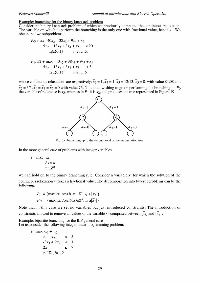
Example: branching for the binary knapsack problemConsider the binary knapsack problem of which we previously computed the continuous relaxation.The variable on which to perform the branching is the only one with fractional value, hence x1. Weobtain the two subproblems:

P0: max 40x2 + 38x3 + 9x4 + x55x2 + 13x3 + 3x4 + x5 $ 20

xi"{0,1}, i=2,…, 5.

P1: 52 + max 40x2 + 38x3 + 9x4 + x55x2 + 13x3 + 3x4 + x5 $ 3

xi"{0,1}, i=2,…, 5

whose continuous relaxations are respectively: x–2 = 1, x–4 = 1, x–3 = 12/13, x–5 = 0, with value 84.08 andx–2 = 3/5, x–4 = x–3 = x–5 = 0 with value 76. Note that, wishing to go on performing the branching, in P0the variable of reference is x3, whereas in P1 it is x2, and produces the tree represented in Figure 19.

x1=1 x1=0

P

0PP1

=1x2 =0x2 =1x3 =0x3

Fig. 19: branching up to the second level of the enumeration tree

In the more general case of problems with integer variables

P: max cxAx $ b

x "Zn

we can hold on to the binary branching rule. Consider a variable xi for which the solution of thecontinuous relaxation x–i takes a fractional value. The decomposition into two subproblems can be thefollowing:

PL = {max cx: Ax$ b, x "Zn, xi $ 1x–i2}PU = {max cx: Ax$ b, x "Zn, xi !4x

–i6}.

Note that in this case we set no variables but just introduced constraints. The introduction ofconstraints allowed to remove all values of the variable xi comprised between 1x–i2 and 4x–i6.

Example: bipartite branching for the ILP general caseLet us consider the following integer linear programming problem:

P: max -x1 + x2x1 + x2 $ 5-3x1 + 2x2 $ 12x1 $ 7xi"Z+, i=1, 2.


30

Figure 20 shows the geometric representation of P and the solution of its linear relaxation, which isgiven by x–1 = 9/5, x–2 = 16/5.

c

x

x2

1

Fig. 20: geometric representation and solution of the continuous relaxation

If we choose to perform the variable x1 we obtain the two subproblems:PL: max -x1 + x2

x1 + x2 $ 5-3x1 + 2x2 $ 12x1 $ 1xi"Z+, i=1, 2.

PU: max -x1 + x2x1 + x2 $ 5-3x1 + 2x2 $ 12x1 $ 72x1 ! 2xi"Z+, i=1, 2.

In Figure 21 the feasible regions of the two subproblems are pointed out.


31

c

x

x2

1P PL U

Fig. 21: geometric representation and solution of the continuous relaxation

ExerciseDevelop the enumeration tree for problem P evaluating the solution of continuous relaxations and making use of thegeometric representation shown in Figure 21.

When developing an enumeration tree for some problems, it might be interesting not to hold on to abipartite branching rule. For example, in an ILP problem of the type

P: max cxAx $ b

x "{1,…,k}n

(i.e., a problem in which variables take integer values in a bounded set), once we detect the variable onwhich to perform the branching (xi ) it might be helpful to carry out the following decomposition:

P1 = {max cx: Ax$ b, x "{1,…,k}n, xi = 1}…Pk = {max cx: Ax$ b, x "{1,…,k}n, xi = k} ,

that is to set the value of the branching variable in turn at all possible values situated in its feasibilityset. In this case we speak of k-partite branching.A k-partite branching rule can also be adopted in certain cases of problems with binary variables, asshown by the following example.Example: branching for the traveling salesperson problemLet G=(N,A) be an undirected complete graph with weights wij!0 associated with arcs; the purpose isto determine the Hamiltonian cycle with least total weight. In Chapter 2 we saw how this problem canbe formulated using binary decision variables associated with arcs. So we might be induced to form anenumeration tree on the basis of a binary branching rule. Yet, it should be noted that the variables aren(n-1)

2 , hence the leaves of the complete enumeration tree will be 2n(n-1)/2, whereas the number offeasible solutions, i.e., the number of Hamiltonian cycles of a complete graph, is (n-1), that is a numberbeing much smaller than the leaves of the tree. This means that a very large amount of leaves willcorrespond to unfeasible solutions, and taking into account their removal might be a heavy task.An alternative branching rule can be of the k-partite type. Let us consider the root node of theenumeration tree and let us suppose we are at node 1 of the graph and we have to start the search. Wehave (n-1) alternatives, that is as many as the nodes still to be visited. So we can open (n-1) branchesof the tree, one for each node following the first. At the following levels of the tree the choices arereduced (one less for each level). until we come to level (n-2) where of course there is no choice. Thereis a correspondence 1:1 between the leaves of the tree and the permutations of n nodes starting withnode 1, thus with the feasible solutions of the traveling salesperson problem.


32

…1nx =113x =1

x12=1

…

=1x 23

Fig. 22: a k-partite branching rule for the traveling salesperson problem

Note that when we choose the node following node i in the cycle (let it be j), we actually set thevariable xij at 1. While making this choice, we implicitly set all variables xih at 0, because we cannothave any other nodes following i in addition to the one we chose.The branching strategy we have just proposed is static and in no way related to the information drawnfrom the computation of the problem relaxation. Let us now propose a second k-partite branching rulebased on the information drawn from the relaxation in which subcycle removal constraints are left out(TSPR). If the solution of the relaxation is unfeasible, this means that there exists a cycle notcontaining all the graph nodes. For more simplicity, let us suppose that the solution of the relaxationinduces a cycle having three nodes {i - j - h}. A branching rule taking into account this piece ofinformation partitions the set of solutions by trying to "split" such cycle, thus preventing that the arcscomposing the subcycle are simultaneously present in the solution. The subproblems that aregenerated are:

P1: {min cx: x"X, xij=0}P2: {min cx: x"X, xij=1, xjh=0,}P3: {min cx: x"X, xij=1, xjh=1, xhi=0}.

ExerciseProve that the branching rule proposed for the traveling salesperson problem partitions the feasible region correctly,without excluding any Hamiltonian cycle.

3.3 Enumeration tree search strategiesA further element characterizing a Branch and Bound algorithm is the criterion according to which wechoose the next node of the enumeration tree to be explored. In general, two fundamental criteria canbe distinguished: the best first and the depth first.The simple Branch and Bound procedure we summarized in Figure 17, due to its recursive nature,makes the choice of immediately and sequentially exploring the nodes generated by the branchingoperation. During the execution of the algorithm two cases may take place at a node of theenumeration tree. In the first case the bound of the node is greater than the best solution value that wasfound (in case of a maximization problem), so a further exploration is needed. This means that thesubproblem is decomposed and the procedure goes on exploring a node having greater depth. In thesecond case the bound provides a feasible solution, sanctions the unfeasibility of the subproblem orverifies that the possible solutions being feasible for the subproblem are of no interest for solving thegeneral problem. In that case, the recursive procedure terminates without further decomposing theproblem and the algorithm goes on exploring another node at a higher level, thus performing a so-called backtracking operation. As it clearly appears, this implementation of the algorithm performs adeep search of the tree (depth first), giving priority to the rapid attainment of a leaf of the tree andtherefore to the rapid generation of a feasible solution, even though nothing guarantees that thegenerated solution is of good quality. A further advantage of this type of enumeration tree searchstrategy is that the memory requirements of the algorithm execution are very small. In fact, during theexecution we will have at most k "open" nodes for each level of the tree, where k is the greatest numberof nodes generated by the branching rule. On the other hand, the main disadvantage derives from thefact that, if no good starting solution is available then, thanks to the bound rule, the subproblemremoval from the enumeration tree becomes more improbable, thus the number of nodes to enumeratecan be very high.In order to lead the exploration of the enumeration tree towards the generation of solutions of goodquality, and thus make the subproblem removal rule more effective, we might choose to explore first


33

the nodes providing a better bound (hence the definition "best first" criterion), which is obviouslyhigher in case of maximization problems. This type of implementation of the algorithm cannot becarried out in a simple recursive form; on the contrary, it implies the introduction of an appropriatedata structure memorizing the nodes still to be explored and from which at each iteration we select thenode with highest bound value. This criterion allows to explore first the portions of the tree that aremore "interesting" and that more probably contain the optimal solution. But unfortunately, due to thecharacteristics of the relaxations, the best bounds are provided by nodes being on a higher level in theenumeration tree. This implies that the number of "open" nodes can be very high (in principle, it isexponential in the number of tree levels) and that the memory requirements of the algorithm executionare heavy.In the literature there are several algorithms of the "hybrid" type as well, which combine the two treesearch criteria. For example, by setting an upper bound to the number of nodes being simultaneouslyopen, it is possible to proceed to a best first search until such bound is achieved and then to continuewith the depth first criterion, which does not affect the use of memory by the algorithm.ExerciseDescribe the pseudocode of the Branch and Bound algorithm formally, according to the best first criterion. What datastructure can be used to memorize the tree nodes, taking into account the selection operations that must be performed?

*4. Notes on computational complexitySo far we have reviewed several optimization problems and we have studied algorithms for solvingthem. We mainly focused our attention on aspects concerning the correctness of algorithms, that is onthe optimality guarantee of the detected solutions. Another fundamental aspect of algorithmic studiesconcerns the efficiency of the proposed algorithms, that is to say an evaluation of their performances,typically in terms of execution time or memory space.In order to present the considerations related to algorithm efficiency with method, we need to introducea few basic definitions. In the following pages the word problem will mean a question expressed ingeneral terms and whose answer depends on a certain number of parameters and variables. Aproblem is usually defined by means of:- a description of its parameters, which are generally left undetermined;- a description of properties having to characterize the answer or the wanted solution.For example, the traveling salesperson problem is specified in the following way: "On an undirectedcomplete graph, where weights are associated with arcs, find the Hamiltonian cycle having the leasttotal weight". The problem parameters are the number of graph nodes (no need to further specify,since the graph is complete) and the matrix of arc weights. The characterization of solutions is givenby the specification of Hamiltonian cycles, and the solution we look for is the one in which the sum ofthe arcs composing the cycle is minimum.

An instance of a given problem P is that particular question obtained by specifying particular valuesfor all parameters of P.Therefore, in the traveling salesperson case, an instance is obtained by specifying the value of thenumber of nodes n and providing as input n(n-1)/2 weights to be associated with the graph arcs.

Formally, an algorithm for solving a given problem P can be defined as a finite sequence ofinstructions which, if applied to any instance p of P, stops after a finite number of steps (i.e., ofelementary computations) providing a solution of the instance p or indicating that the instance p has nofeasible solutions.4.1 Computational models and complexity measuresPreviously in the course, notably in Chapter 2, we measured the efficiency of an algorithm in a ratherinformal way; but in order to study algorithms from the viewpoint of their efficiency, i.e., theircomputational complexity, we need to define a computational model.Classical computational models are the Turing Machine (historically, the first one to be proposed), theR.A.M. (Random Access Machine), the pointer Machine, etc.A good compromise between simplicity and versatility is the R.A.M.A R.A.M. consists of a finite program, of a finite set of registers, each of which can contain one singleinteger (or rational) number, and of a memory of n words, each of which has only one address(between 1 and n) and can contain one single integer (or rational) number.In a step a R.A.M. can:- perform one single (arithmetical or logical) operation on the content of a specified register,


34

- write in a specified register the content of a word whose address is in a register,- store the content of a specified register in a word whose address is in a register.It is a sequential and deterministic machine (the future behavior of the machine is univocallydetermined by its present configuration).

Given a problem P, its instance p and an algorithm A for solving P, we call computational cost (orcomplexity) of A applied to p a measure of the resources used by the computations that A performs ona R.A.M. in order to determine the solution of p. In principle, the resources are of two types: engagedmemory and computing time. Supposing that all elementary operations have the same duration, thecomputing time can be expressed as the number of elementary operations performed by the algorithm.Since the most critical resource is quite often the computing time, in the following pages thecomputing time will be mainly used as a measure of algorithm complexity.

Given an algorithm, we need to have at our disposal a complexity measure allowing a syntheticevaluation of the good quality of the algorithm itself as well as, possibly, an easy comparison of thealgorithm with alternative algorithms. It is not possible to know the complexity of A for each instanceof P (the set of the instances of a problem is generally unbounded), nor would this be of any help inpractice. We try therefore to express the complexity as a function g(n) of the dimension, n, of theinstance to which the algorithm is applied; yet, since there are usually many instances of a specificdimension, we choose g(n) as cost needed to solve the most difficult instance among the instances ofdimension n. This is defined worst-case complexity.We obviously need to define the expression "dimension of an instance" more precisely. We calldimension of an instance p a measure of the number of bits needed to represent the data defining pwith a “reasonably” compact coding, i.e., a measure of the length of its input. For example, in a graphwith n nodes and m arcs, nodes can be represented by means of integers between 1 and n, and arcs bymeans of a list containing m pairs of integers (the arc connecting nodes i and j is defined by the pair(i,j)). Then, leaving out the multiplicative constants, it will be possible, as the number of nodes and arcschanges, to take as measure of the dimension of the graph coding the function mlogn; in fact, logn bitsare sufficient to represent integers being positive and not greater than n1. For more simplicity, in thefollowing pages we will leave out, beside multiplicative constants, sublinear functions as well, such asthe logarithm function; in that case we say that m is the input length for a graph with m arcs. In theformulated hypotheses, the input length measure does not change if we use a basis coding b>2.Otherwise, if we use a unary coding, the input length in the considered example becomes nm, thusincreasing significantly.At this point, the previously introduced function g(n) has been defined rigorously enough. In practice,however, it continues to be difficult to be used as a complexity measure; in fact, the evaluation of g(n)for each given value of n proves to be difficult, if not practically impossible. The problem can besolved by replacing g(n) by its order of magnitude; then we speak of asymptotic complexity.Given a function g(x), we can say that:i) g(x) is O(f(x)) if there exist two constants c1 and c2 such that for each x we have g(x) $ c1f(x)+c2;ii) g(x) is :(f(x)) if f(x) is O(g(x));iii) g(x) is ;(f(x)) if g(x) is at the same time O(f(x)) and :(f(x)).

Let g(x) be the number of elementary operations performed by an algorithm A being applied to themost difficult instance – among all instances having input length x – of a given problem P. We can saythat the complexity of A is an O(f(x)) if g(x) is an O(f(x)); similarly, we can say that the complexity ofA is an :(f(x)) or a ;(f(x)) if g(x) is an :(f(x)) or a ;(f(x)).

When we propose problem solving algorithms we always aim at getting a polynomial complexity inthe input dimension. Unlike exponential algorithms, a polynomial algorithm is considered to beefficient in practice. The following tables clarify the reason of this distinction. Table 1 shows theexecution times (for different complexity functions) on a computer performing one million elementaryoperations per second; Table 2 indicates improvements that can be obtained (in terms of dimensions ofsolvable instances and for different complexity functions) following computer technologyimprovements; with xi we indicated the dimension of an instance today solvable in one minute for thei-th complexity function.

(1) In general, if not differently indicated, in case a problem's data are composed of n numbers, we will consider thenumber of bits needed for the coding in binary of the numbers themselves as being limited by logn.


35

Dimensions of the instanceFunction n=10 n=20 n=40 n=60

n 10-5 sec. 2×10-5 sec. 4×10-5 sec. 6×10-5 sec.n3 10-3 sec. 8×10-3 sec. 6.4×10-2 sec. 2.2×10-1 sec.n5 10-1 sec. 3.2 sec. 1.7 min. 13 min.2n 10-3 sec. 1 sec. 12.7 days 36.6×103 years3n 6×10-2 sec. 1 hour 4×105 years 1.3×1013 years

Table 1: execution times on a computer performing 106 operations per second according to input dimension

Complexityfunction

Present-daycomputer

100 timesfaster

10000 timesfaster

n x1 100 x1 10000 x1n3 x2 4.6x2 21.5x2n5 x3 2.5x3 6 .3x 32n x4 x 4 + 6.6 x4 + 13.23n x5 x 5 + 4.2 x5 + 8.4

Table 2: increment of input dimensions according to computer speed and within the same execution time

In Table 1 we can notice how, in case of polynomial algorithms, the execution time grows according toinput dimensions but remains at acceptable levels, whereas in case of exponential algorithms such time,though still competitive for small instances, soon becomes unsustainable. This difference appears inTable 2 as well, where polynomial algorithms benefit from computing speed progress increasing by amultiplicative factor the input dimension of instances solvable in one minute, whereas in case ofexponential algorithms the progress is given by an additive constant.In Chapter 2 we examined the complexity of several algorithms, some of which – for example thegraph search algorithm, the algorithms for determining the shortest-path tree, the Edmonds-Karpaugmenting-path algorithm – are evidently polynomial. A clearly exponential algorithm is the Branchand Bound algorithm we already presented in this chapter: in the worst case it must explore the wholeenumeration tree which is exponential in the number of variables.Actually, in the classification of algorithms according to their computational complexity we have anintermediate range. Consider for example the negative cycle removal algorithm for a minimum costflow problem or, for the same problem, the algorithm of successive shortest paths. In the evaluation ofthe complexity of these algorithms, we have a polynomial among whose parameters there is not onlythe input dimension, but also a term relative to data (maximum capacity or maximum cost of arcs).For example, we have a complexity of O(nm2CmaxUmax) for the negative cycle removal algorithm. IfCmax and Umax take particularly high values, the complexity grows, and considering that Cmax andUmax are codified "in binary", the complexity grows exponentially in the input dimension. Yet, ifinstead of having recourse to a binary coding, we "trick" and codify the input with a unary code, thenthe complexity is polynomial in the input dimension, thus making our algorithm fall into the class ofpolynomial algorithms.

An algorithm is said to be pseudopolynomial if it can solve one of these problems in polynomial timein the length of the input codified “in unary”.ExercisesClassify the algorithms we saw in Chapter 2 according to the distinctions: "polynomial", "exponential" and"pseudopolynomial". In particular, into which class does the capacity scaling algorithm for maximum flow fall?

4.2 Tractable and untractable problemsIn light of the complexity-based algorithm classification we introduced previously, we can try toclassify problems as well according to the algorithms for solving them. Problems for which there existalgorithms whose complexity is an O(p(x)) with p(x) being a polynomial in the input dimension x aresaid to be tractable and problems for which such an algorithm does not exist are said to beintractable.The critical point of this criterion of classification lies precisely in stating that for a certain problemthere exists no polynomial solution algorithm. If we cannot find an efficient algorithm for a certainproblem, to what extent is this due to its real difficulty and to what extent to our little capacity? This


36

question, which makes the classification rather delicate, was only solved in the early Seventies with thetheory of computational complexity.In order to perform a more rigorous classification we have to refer to problems in decisional form, thatis to problems implying the answers YES or NO. Problems of this kind are, for example, thesatisfiability problem we saw in Chapter 1 and the graph connection problem we saw in Chapter 2.Note that an optimization problem can always be reduced to a problem in decisional form. Considerfor example the problem:

P: max { cx: x"F}.

By introducing a parameter k, the decisional version Pk of problem P is the following:

Pk : { x"F, cx ! k} % ø ?

whose answer is a YES or a NO, and wishing to certify the answer YES we just need to provide asolution x"F such that cx ! k.If an efficient algorithm for solving problem Pk (for any value of k) is available, we can efficientlysolve problem P as well. In fact, we just need to perform a binary research on the optimal solutionvalue, solving a decisional problem Pk at each step and refining the research according to the positiveor negative answer of Pk. In case of positive answer we concentrate our research on values beinggreater than k, otherwise we seek the solution among those having value smaller than or equal to k. If

O(p(n)) is the complexity of the algorithm solving Pk, with n as input dimension, and (_K, _K) are an

underestimation and an overestimation of the optimal solution value of P, the complexity of this binary

research algorithm is O(log (_K - _K) p(n)). Hence, if p(n) is a polynomial in n, then also the binary

research algorithm continues to be a polynomial algorithm.Example: set of maximum cardinality independent nodesGiven an undirected graph G=(N,A), we call a set of independent nodes a subset S#<, such that foreach pair of nodes i and j belonging to the independent set, there exists no corresponding arc in A.Hence

ISP: max { |S|: ,i,j"S, (i,j)=A},

and the corresponding decisional version, given a bound k>0, is:

ISPk : { S: ,i,j"S, (i,j)=A, |S|! k} % ø ?

An important class of problems is the NP class, which consists of all decisional problems certifiablein polynomial time by a R.A.M. machine. This means that, given any instance of a decisional problemP and a solution x, there exists a polynomial algorithm that checks if the given solution is an answerYES for P.SAT exampleIn Chapter 1 we introduced the satisfiability problem (SAT) which, as we shall see, plays afundamental role in the theory of computational complexity. It is given a logical formula in conjunctivenormal form A=C1>…>Cm in which each clause Ci is a disjunction of literals (±Pj) and theelementary propositions composing the formula are P1, …, Pn. The problem consists in finding anassignment of truth values to the elementary propositions P1, …, Pn rendering the formula true. Theproblem is of the decisional type, the input dimension is O(mn), since that the formula is composed ofm clauses, each of which contains at most n literals. The certificate of an answer YES is given by thevalue assignment, therefore it has length O(n), hence SAT belongs to NP.Example: connected graphLet us examine the problem of determining the connectivity of a digraph that we saw in Chapter 2.Given a digraph G=(N,A) and two nodes s and t of N, the problem consists in establishing if thereexists a path directed from s to t. The problem is obviously of the decisional type. Denoting by n andm the number of nodes and the number of arcs of the graph, respectively, then the input dimension isO(n+m). The certificate of an answer YES is given by the path itself that connects s to t and that canbe therefore represented by a sequence of at most n-1 successive arcs (s,i1), (i1,i2), …, (ir,t). So, we can


37

conclude that the problem is in NP. Note that in this case the answer NO is polynomially certifiable aswell; in fact, the non- existence of a path between s and t is proved by the existence of a partition of theset of nodes N into two subsets Ns and Nt such that s"Ns, t"Nt and all the arcs with endpointsspanning the partition have tail in Nt and head in Ns.Example: set of independent nodesLet us consider again the problem of the set of maximum cardinality independent nodes (ISP) we havejust presented. A possible solution S is given by a subset of nodes, hence the input into thecertification problem, given by the graph G=(N,A), by the subset S and by the constant k, hasdimension O(m+n). In order to verify whether S really is a solution to the problem, first of all we haveto verify that |S|!k and afterwards, by sequentially examining each arc of A, we can verify whether bothendpoints are in S. If not, the given solution is an answer YES. The complexity of this operation isO(m), so the problem of the maximum set of independent nodes in decisional form is in NP.ExerciseHow can we certify an answer NO to the satisfiability problem? Is it possible to give a polynomial certificate of it?

A subset of NP class is the so-called P class of problems solvable in polynomial time, which containsall decisional problems for which there are polynomial complexity algorithms that solve them(polynomial problems).Example: connected graphIn Chapter 2 we saw that by means of an algorithm searching the graph from node s we could providea solution to the connection problem in O(m) time. This means that the problem belongs to the Pclass.

A very important question is whether in NP there are problems we can guarantee as not belonging to Pas well, that is whether P%NP. For example, the SAT problem and the decisional version of the ISPproblem, for which up to now no polynomial solution algorithms have been provided yet, are in P: arewe not skillful enough to find an algorithm or are they intrinsically difficult? No one has been able toanswer this question, although it is more than likely that the answer is positive, i.e., that actually P%NP.4.3 NP-complete problems and NP-hard problemsWith the purpose of characterizing intrinsically difficult NP problems in some way, a specific subsetof problems was introduced. This class, known as NP-complete problems, represents the core of theNP problems that are considered to be difficult. In order to define this class formally we need tointroduce the concept of polynomial reduction, which allows to relate two problems.

Though apparently quite different, many problems can be related one to the other. Given twodecisional problems, P and Q, we say that P is reduced to Q in polynomial time (thus we write P ? Q)if, assuming the existence of an algorithm AQ that solves Q in constant time (i.e., independent from theinput length), there exists an algorithm that solves P in polynomial time by using AQ as a subprogram.In this case we speak of polynomial reduction of P to Q.Example: reduction from Hamiltonian cycle to TSPLet us show how the problem of the existence of an Hamiltonian cycle (HC) on any symmetric graphG=(N,E) can be polynomially related to the traveling salesperson problem (TSP) on completesymmetric, weighted graphs, in its decisional version; in other words: how to determine the existenceof an Hamiltonian cycle with weight smaller than or equal to a pre-set value k. Let ATSP(N,c,k) be analgorithm that, given a set of nodes N and a real function c : N×N@ R, returns YES if there exists aset of arcs forming an Hamiltonian cycle with cost $ k, and NO otherwise. The following algorithmsolves HC polynomially, supposing that the complexity of ATSP(N,c,k) is O(1):

Procedure Hamiltonian_Cycle(N,E):begin

for all i,j"N do if (i,j)"E then c(i,j) := 0 else c(i,j) := 1;return ATSP(N,c,0)

end.Hence, we can state that HC ? TSP. In practice, this means that HC is no more difficult to solve thanTSP. In fact, if there existed a polynomial algorithm for TSP, hence TSP"P, then also HC"P.


38

Conversely, if we could prove that HC admits no polynomial algorithms, the same would apply to TSPtoo. These important considerations are summarized in the following property:Property 4.1- If P ? Q and Q " P, then P " P.- If P ? Q and P = P, then Q = P;

The relation ? has the following properties:

i) is reflexive: P ? P;ii) is transitive: P ? Q and Q ? R + P ? R.

Precisely the transitivity of the reduction is helpful in defining the class of NP-complete problems andin proving in a practical way that a problem is NP-complete.Definition 4.2A problem Q is said to be NP-complete if Q " NP and if for each P " NP we have P ? Q.

Following the definition, the task of proving the NP-completeness of a problem might appearimpossible, because it requires countless reductions. In 1971 Cook solved this difficulty bydemonstrating that any instance of a problem P of NP turns into an appropriate logical formula withpolynomial length in the input dimension of P. We can deduce that any problem in NP is reduced toSAT in polynomial time.Theorem 4.3 (Cook, 1971)Each problem P " NP is polynomially reduced to SAT (satisfiability problem).

From Cook's theorem follows that SAT is an NP-complete problem and that it constitutes a majorpoint of reference. The theorem's proof, which is rather technical, represents a milestone in thecomputability theory and should not be missing from the store of knowledge of a good informationscientist. For deeper interest, we refer to the proof that appears in [C. H. Papadimitriou and K.Steiglitz, 1982].

NP-complete problems have the property that if there exists a polynomial algorithm for one of them,then all problems in NP are necessarily solvable polynomially, so we would have P = NP. In a sense,such problems are the most difficult problems in NP.Figure 23 shows the relations between NP, P and the class of NP-complete problems.

NP

NP-complete

P

Fig. 23: scheme of problem classification

Once proved that SAT is NP-complete, we can prove that a problem P belongs as well to the class ofNP-complete problems by simply reducing SAT to P, and according to the transitivity of the reductionwe will obtain that any problem in NP is reduced to P. Note that at this point P too becomes useful forproving the NP-completeness of other problems. Thus, in order to prove a problem's NP-completeness, it generally suffices to take any NP-complete problem as reference and find an


39

appropriate reduction. Let us give an example while finding a polynomial reduction from SAT to theproblem of the set of independent nodes (ISP).Theorem 4.4 [Karp 1972]ISP is NP-complete.ProofFirst of all note that, as we already saw, ISP is in NP because a solution of an instance YES can beverified in polynomial time.Consider now an instance of the SAT problem – i.e., the problem of determining whether a givenlogical formula A admits an assignment of truth values that renders it true – which, as we know,belongs to the class of NP-complete problems. For more simplicity, we can assume that A is inconjunctive normal form, i.e., is specified by a set of clauses C1 >…>Cm, each of which is given bythe disjunction of literals (direct or negated logical variables): Ci = ±X1 A…A±Xik. Globally, the set oflogical variables is given by {X1, …, Xn}.Now let us build an undirected graph G=(N,E) corresponding with the formula A. For each clause weintroduce as many nodes as the literals composing it. We also introduce arcs connecting the nodes ofeach clause to one another, thus forming many complete subgraphs Gi=(Ni,Ei) for each clause Ci. Thegraph can be completed by introducing arcs E' connecting, in pairs, the nodes relative to the logicalvariables that appear with different signs in different clauses. Note how in the following example wec a n b u i l d t h e g r a p h o f F i g u r e 2 4 f r o m t h e f o r m u l a :A=(X1A¬X2AX4)>(X3A¬X4)>(¬X1AX2A¬X3)>(X2A¬X3).

X1¬

¬ 2X

3X¬

3X¬

4XX1

3X

X2

X2

4X¬

Fig. 24: instance of a set of independent nodes that is associated with a logical formula

If the graph, formed in this way, has a set of independent nodes I with cardinality m, then we havedetected a set of m literals, each belonging to a different clause and compatible two by two. We canobtain an assignment of truth values as follows. We assign value true to variables corresponding tonodes in I if variables are direct, and we assign value false if variables are negated; we assign anarbitrary value to other possible variables to which no value was assigned.Conversely, if there exists an assignment of truth values rendering A true, thus rendering each of mclauses true, then we can build a set of independent nodes by choosing a node corresponding to a trueliteral for each clause. /

In the example of Figure 24 there exists a set of four independent nodes that are associated withliterals X1 in the first clause, ¬X4 in the second one, X2 in the third and the fourth one. An assignmentof truth values relative to this set of nodes is X1= X2 = true, X4 = false. This assignment of values tovariables renders formula A true for any value of X3.ExerciseGiven an undirected graph G=(N,E), let us consider the problem of determining whether in G There exists a completesubgraph (called clique) having cardinality k. Prove that such problem is NP-complete by making use of a techniquesimilar to the one used for ISP.


40

A problem having as particular case an NP-complete problem has the property of being at least asdifficult as NP-complete problems (except for a polynomial multiplicative function). A problem of thistype is called NP-hard. It should be observed that an NP-hard problem can also not belong to NP. Forexample, optimality problems whose decisional version is an NP-complete problem are NP-hard.Thus, the optimization version of ISP is NP-hard.

When we speak of input length we assume that the way used to codify the data defining the problemwas reasonably compact. For example, we can assume that if x is the problem length with the codingthat was used and y the length with any other coding, then x is an O(f(y)), where f is a polynomial(possibly with degree 1).For example, the integer number a has length x = loga if codified “in binary”, whereas it has length y= a if codified “in unary”. Clearly, the coding “in unary” is not acceptable with respect to the criteriapresented above; in fact y grows exponentially with x.Yet, it should be noted that there exist problems that are polynomially solvable in the input length ifcodified “in unary”, whereas they are not so with more compact codings. Such problems are in asense easier than those requiring exponential algorithms apart from the input coding. For example, wesaw that the knapsack problem admits a pseudopolynomial algorithm that makes use of the search fora longest path on an appropriate graph.We call NP-complete in the strong sense an NP-complete problem for which there exist nopseudopolynomial algorithms. Similarly, we call NP-hard in the strong sense an optimization problemhaving as particular case an NP-complete problem in the strong sense.

A very useful tool for determining results pertaining to computational complexity of combinatorialproblems is the compendium edited by P. Crescenzi e V. Kann:http://www.nada.kth.se/~viggo/wwwcompendiumThe Web site offers a synthetic historical memory of complexity results appearing in the literature, it isregularly updated and presents new results, new problems and an up-to-date bibliography.5. Approximate algorithmsWhen confronted with instances of an NP-hard problem, we know that solution time is likely to belong. It frequently happens, however, that the solve time available is limited, so we have to diminish ourambitions and be satisfied with a good solution, not necessarily optimal but quickly obtained.Moreover, note that optimality is quite often an important property from the theoretical viewpoint, butits meaning is uncertain in practice. In Chapter 1 we saw that there is always some distance betweenreality and model. Such distance derives also from the difficulty (or quite often even the impossibility)to know exactly all the quantities that are involved; thus, the coefficients appearing in the model areencumbered by errors that in most cases are substantial: some constraints may have been left out, etc.In several cases, this contributes to make the search for the "theoretical optimality" of little significancefrom the practical point of view.In such cases we make use of approximate algorithms, also known as heuristics because they utilizethe knowledge of the particular problem's structure and of the characteristics of optimal solutions.When using heuristic algorithms we should (although it is not always easy or possible) perform ananalysis of the error we are making and accept the obtained solution instead of the optimal one.Consider the problem min {c(x): x"F).Let A be an algorithm for such problem and xA the (not necessarily optimal) solution it provides, andlet:

zOPT = {min c(x): x " F},

zA = c(xA).

We define:

absolute error EA = zA - zOPT

relative error RA = zA - zOPT

zOPT

An algorithm A is B-approximate, with B>0, if:


41

RA $ B .

An approximation scheme is an approximate algorithm such that, for each B>0, it produces a solutionwith RA $ B. The complexity of such an algorithm is obviously a function of the wanted approximationB (growing with 1/B).An approximation scheme is said to be:- polynomial, if its complexity is polynomial in n (input dimension);- fully polynomial, if its complexity is polynomial in n and in 1/B.

An interesting branch of the theory of complexity concerns problem approximability. In case of NP-hard problems, this means determining particularly difficult classes which do not admit polynomialapproximation schemes.

Like when dealing with the modeling of decisional problems, in the case of heuristics as well it isdifficult to systematize the exposition and provide an infallible "recipe" for producing goodalgorithms. The best heuristic algorithms are actually the fruit of experience, at times of luck, and ofknowing the specific characteristics of the different problems. Considering the difficulty of the task –which would require a complete course – and the little space available, we will just describe two verygeneral algorithmic schemes that we already applied to several problems we saw in the previouschapters. The first one is the class of greedy algorithms that iteratively build feasible solutions withoutever going back to choices made previously. The second one is the class of local-search algorithmsthat, starting from a feasible solution, seek possible better solutions obtained by making slight changesin the given solution. The two types of algorithm can be used in sequence by means of a greedyalgorithm generating a feasible solution to be improved afterwards using a local-search algorithm.5.1 Greedy algorithmsBefore presenting the formal description of the scheme for algorithms of the greedy type, let usanalyze a simple example and try to build a relevant solution relying on "common sense".Example: constructive algorithm for the knapsack problemConsider the instance of the knapsack problem in the burglar example of Chapter 1:

max 7x1 + 2x2 + 4x3 + 5x4 + 4x5 + x65x1 + 3x2 + 2x3 + 3x4 + x5 + x6 $ 8x1, x2, x3, x4, x5, x6 " {0, 1}.

A presumably good, though generally not optimal, solution can be obtained by proceeding accordingto the following informal scheme. Indexes of objects are arranged in a descending unit profit order;then variables are examined following the established order: each variable is assigned value 1 if addingthe object does not violate the capacity constraint, otherwise it is assigned value 0, and in fact thecorresponding object is definitively discarded.In the examined case, the steps that the described method would take are the following:1. The object having greater unit cost is the fifth; its ratio cost/weight is equal to 4; as the object has

weight 1 and the residual capacity of the knapsack at this moment is 8, we set x5=1, thus leavingenough room in the knapsack for 7 further weight units.

2. The following object in the selected order is the third; its unit cost is 2; its weight is less than theresidual capacity, so we set x3=1; the residual capacity of the knapsack descends therefore to 5.

3. The following object is the fourth; its unit cost is 5/3; in this case too, since there is enoughcapacity available, we can set x4=1; the knapsack still has a residual capacity of 2 units.

4. The following object is the first; its unit cost is 7/5 but its weight (5) is greater than the residualcapacity of the knapsack (2), so the corresponding variable x1 is set at zero.

5. The following object is the sixth, which has unit cost 1; since its weight is 1, we can set x6=1; theknapsack still has a residual capacity of 1 unit.

6. The last object to be examined is the second; since it has weight greater than the residual capacityof the knapsack, it is discarded and the variable x2 is set at zero.

The obtained solution is therefore (0, 0, 1, 1, 1, 1), with cost 14 and total weight 7. It clearly appearsthat this solution is not optimal: in fact, the solution (1, 0, 1, 0, 1, 0), with total weight 8, has cost 15.Thus, the described algorithm does not guarantee the optimality of the solution; yet, it has theadvantage of being simple to implement and computationally very efficient, because its complexity –except for the ordering of objects – is linear in the input dimension.


42

An algorithm of this type is called greedy algorithm. it is a kind of algorithm that determines thesolution through a sequence of partial decisions (locally optimal), without ever going back to alreadymade decisions and modifying them. These algorithms are easy to implement and considerablyefficient from the computational point of view, but, with a few important exceptions, do not ensure theoptimality and at times not even the feasibility. The class of problems that can be optimally solved bygreedy algorithms is known as the class of matroids. For a deeper knowledge of matroids we refer toLawler's book.

In order to present these algorithms formally, we usually refer to problems represented in the form ofsystems of independent sets.We detect a set E (ground set) that can be considered as the set of elements composing the solution ofthe examined problem. In the case of the knapsack problem the set E is given by the set of objects tochoose. Further, we detect the set F, which is given by a family of subsets of E (F # 2E ), such thatthe property of closure by inclusion holds:

(A # B) e (B"F) + A"F.

the set F represents the set of all partial solutions being feasible for the problem. So, we call:F a family of independent sets,(E,F) a system of independent sets.

A set I"F is called a maximal set if:

e"E \ I @ I - {e} = F.

Given a function

c: 2E @ R,

we call a problem associated with (E,F) the following optimization problem:Determine a maximal set I"F such that:c(I) ! c(Y), , Y"F and maximal.

Similarly, we can make a minimization problem correspond with (E,F).It is given the optimization problem associated with the system of independent sets (E,F) with objectivefunction c; an algorithm of the greedy type builds the set X"F (the solution of the problem), startingfrom the empty set and, at each step, inserting in it the most "promising" element of E among those notviolating the set independence.This type of algorithm, in its most general form, is described by the following procedure greedy:

Procedure greedy:begin

X := Ø; S := E;repeat

e := Best(S); S := S \ {e};if Ind(X,e) then X := X -{e}

until S = Øend.

The algorithm makes use of the two subprocedures Best and Ind:Best provides the best element of S according to a pre-set criterion (for example the element withminimum cost in the case of the minimum cost spanning tree problem, or the element with themaximum ratio of vi/pi in the knapsack problem).Ind is a logical function that is defined as follows:

Ind(X,e) = '()(*true , if X -{e }" F,

false, otherwise.


43

In the knapsack example considered at the beginning of the paragraph, F is the set of all subsets ofelements whose total weight is less than or equal to the knapsack's capacity (i.e., the set of all feasiblesolutions).Let us now analyze the complexity of the procedure greedy.Let |E| = n; we denote by h(n) the complexity of Best and by k(n) the complexity of Ind. Then, thecomplexity of the whole procedure is O(n(h(n)+k(n))). Suppose that the elements of E are ordered atthe beginning, hence at each step Best provides the first among the remaining elements; then thecomplexity becomes O(nlogn+nk(n)).Example: set coveringIn the set covering example, let there be a set I of elements and a family J={J1,…,Jm} of subsets of I.A cost cj is associated with each subset Ij. The purpose is to determine a selection of subsets of thefamily such that each element of I appears in at least a selected subset and the sum of the costs of thechoice that was made is minimized. Such problem is NP-hard, as it is confirmed in the summaryavailable at the Web site we mentioned in the pages concerning problem complexity. Let us formulatethe problem in terms of system of independent sets. In this case the set E is given by subsets of familyJ, or alternatively by the set of indexes {1,…,m}. The family of independent sets F is given by the setpower of E, hence by the set of all possible subsets of indexes. In fact, note that the solution X=E too,although probably quite inefficient, is feasible for the set covering. Wishing to specify the greedyalgorithm, we just need to define the details of the functions Best and Ind. The Best can be led by costcj if we choose the minimum cost subset in S, or it can be led by the set cardinality if we give priorityto larger subsets, or else a compromise between these two criteria can be found if we give priority tosubsets whose cost for each element is minimum:

Best(S) = argmin{cj: j"S}

Best(S) = argmax{|Jj|: j"S}

Best(S) = argmin{ cj|Jj|: j"S}

On the other hand, as any subset of indexes represents a partial feasible solution, the function Ind,always returns true and no filter must be applied. In this way we obtain a correct greedy algorithm.However, wishing to go more into details, we see that the algorithm, just as it is specified above, canyield "redundant" solutions, i.e., solutions in which there are some subsets merely containing elementsthat are already covered by other selected subsets. To overcome this difficulty we can modify the Indin the following way:

Ind(X,j) = '()(*true , if in Jj there are elements of I that are not contained in any Ji for i"X,

false, otherwise.

This Ind ensures that, at each iteration, the greedy algorithm for the set covering increases the set ofcovered elements, thus it actually prevents redundant solutions. Note that, according to how thefunction Best was described, the criteria adopted to choose a subset are static; therefore, as it was thecase in the knapsack problem, we could make use of a starting ordering of all subsets according to theparticular function that was chosen. Yet, it should be observed that in the second and the thirddefinition of the Best we refer to the subset cardinality. If, instead of considering the cardinality in anabsolute sense, we considered the cardinality of the set of the new elements that would be added to thecurrent solution, we could prevent redundancies, without having to specialize the function Ind, and atthe same time we would obtain a more sophisticated criterion of choice. This "dynamic" criterion ofchoice would make the starting ordering useless and, at each call of the Best, would require a completescansion of the set S, thus making the algorithm complexity slightly heavier.

The greedy algorithm, in its general form, can be applied to many problems without any particularimplementative tricks, as we saw for the knapsack and the set covering problems. In the case of morecomplex problems, it can be worth while to specialize the greedy in order to make full use of thestructure and of the specific features of the examined problem. Let us look at the case of the travelingsalesperson problem.


44

Example: greedy algorithms for the traveling salesperson problemThe problem is specified by an undirected complete graph G=(N,A) with costs associated with arcscij!0. A banal way of yielding a greedy algorithm for the traveling salesperson problem proceeds byapplying the general rules described above; so, considering that a solution can be viewed as a subset ofarcs, we can define E=A and F={H#C: H is a Hamiltonian circuit or a subset of the latter and notnecessarily connected}. The Best(S) just returns the arc of minimum cost among those in S:

Best(S) = argmin{cij: (i,j)"S}

and the Ind verifies whether adding an arc to the current solution allows to reach the end of thealgorithm with a Hamiltonian circuit:

Ind(X,(i,j)) = '()(*true , if X-{(i,j)} does not contain nodes with three incident arcs or subcycles,

false, otherwise.

The defect of this algorithm is that it chooses the best arcs at once, but then must hold on to choicesthat may be arbitrarily bad.Another version of greedy algorithm for the TSP slightly deviates from the general scheme describedabove, although it maintains the feature of building a feasible solution incrementally by making locallyoptimal choices.The idea is to start from a solution already being a circuit, though not Hamiltonian, and increase it ateach iteration by adding the node implying the shortest deviation. Let (i,j) be the arc of minimum costof the graph; we can take the circuit i-j-i as starting solution. At each iteration we consider each arc(h,k) of the circuit and each other node y of the graph which is not included in the solution yet; furtherwe compute the global cost of the deviation: shky = chy + cyk - chk, and we choose the triplet h,k,yminimizing the value of the deviation shky and we insert the node y in the most advantageous point ofthe circuit, hence between node h and node k. Using the sequence of nodes of the circuit asrepresentation of the solution X, the functions specifying the algorithm become:

Best(S,h,k) = argmin{shky = chy + cyk - chk,: y=X,(h,k)"X}Ind(X, y, h, k) = true

where the Best returns, beside the index of the node to be inserted, also the pair of nodes (h,k)(adjacencies of the current circuit) into which the new node must be inserted. According to thiscriterion of choice, the Ind becomes superfluous. This algorithm is known in the literature as nearestinsertion.ExerciseProvide an efficient data structure to implement the nearest insertion algorithm.Countless constructive algorithms for the TSP have been proposed over the years, all referring to agreedy logic. Let us look at a further greedy algorithm that makes use of the result of one of theequally numerous relaxations of the problem. Consider the relaxation of the TSP obtained by leavingout the subcycle removal constraints. As we saw previously, the problem corresponds to anassignment on bipartite graph and its result is a circuit cover of graph G on which the TSP problem isdefined. If we are lucky, we obtain only one Hamiltonian circuit corresponding to the optimal solutionof the problem; if not, we will have many subcircuits. The algorithm examines these circuits and"patches them up" in pairs, until it obtains only one circuit.

i

j h

ki

j h

k

Fig. 25: the "patching" of two circuits

Figure 25 illustrates the process of patching up two circuits. We detect two arcs (i,j) and (h,k) in twodifferent circuits which will be replaced by the arcs (i,k) and (j,h) (or (i,h) and (j,k)). The new solutionwill have an additional cost of P(i,j,h,k)=cik + cjh - cij - chk. Algorithms based on this technique arecalled "patching" algorithms; at times, instead of costs, we use the reduced costs resulting from the


45

solution of the assignment problem. It is not difficult to define the details of a greedy algorithm basedon patching.ExerciseSpecify the representation of the partial solution as well as the functions Best and Ind for a greedy algorithm based onthe patching technique.

Greedy algorithms are usually extremely fast, but yield only one solution. When approaching acomplex problem, the time available may be enough to allow attempts at producing more than oneheuristic solutions. In such situations, however, the greedy is of no help because, if called repeatedlyon the same input, it always yields the same solution. A way to avoid this defect is to render the choiceof the Best non-deterministic, so that if the algorithm is called more than once, at each execution – atleast in principle – different choices are made and alternative solutions are generated. This idea formsthe basis of GRASP (Greedy Randomly Adaptive Search Procedure) algorithms. Using our greedyprocedure scheme, the only modification concerns the function Best. The new function, summarizedbelow, takes as input the set S of elements that are candidate to enter the solution, like in the case of thetraditional greedy, but also a parameter 0<D<1 establishing a deviation threshold from the value of thebest choice. The Best_GRASP takes into consideration elements not deviating from the best in S bymore than D%, randomly selects one of these and returns it as result.

Function Best_GRASP(S,D)begin

v := min (cj: j"S}S' := {j: cj ! v (1-D)} {selection of elements being no worse than Dv in relation to the best}return (random_selection(S'));

end.In practice, GRASP algorithms, that are based on the simple idea we summarized above, contain manyother "ingredients" and expedients, and are usually accompanied by appropriate local-searchalgorithms. For deeper study of the subject, see [], or look at the Web site of Mauricio Resende:http://www.research.att.com/~mgcr/grasp/index.html5.2 Local-search algorithmsLocal-search algorithms examine a feasible solution and iteratively try to improve it. During the coursewe have been dealing with various local-search algorithms, such as augmenting-path algorithms for themaximum flow problem, or the negative cycle removal algorithm for the minimum cost flow problem,or again the Primal-Dual Simplex algorithm for linear programming. These algorithms arecharacterized by the fact that at each step they examine a feasible solution, seeking a better one amongthose that are "near" to it, thus restricting the search (hence the term "local") to a neighborhood of thecurrent solution. So, we can try to provide a general description of this algorithmic paradigm with theaim of using it as a guide for yielding new algorithms for a variety of problems, as we did for thegreedy.In general, a local-search algorithm is characterized by the following operations:- we determine a starting feasible solution x0;- we iteratively explore a sequence of feasible solutions, x0, x1,…, xk,…, and we stop as soon as one

of the detected solutions is recognized as being an optimal or not improvable solution.The search for the solution improving the current solution xi is performed in a subset of feasiblesolutions near to xi, which is called neighborhood of xi and is denoted by I(xi). In general, whendefining a neighborhood, the following rules are to be considered, recalling that F indicates the set offeasible solutions of the problem:1) x " F + x " I(x);2) x, y " F + E {x0, x1, ..., xp} # F, con x0 = x, xk " I(xk-1), k = 1,…, p, xp = y.The first rule implies that each solution belongs to its own neighborhood, so as to ensure a stoppingcondition for the algorithm. The second rule, more difficult to verify, ensures that, given any twosolutions, it is possible to "migrate" from one to the other through a sequence of modificationscompatible with the definition of neighborhood, even though the resulting sequence of solutions is notnecessarily best-oriented. This rule, at least in principle, guarantees that it is possible to generate anysolution from any starting solution. Occasionally, however, the constraints of the examined problemare so stringent that they cannot guarantee this second property for a certain neighborhood. Later inthe course we will see how to overcome this difficulty.


46

A further essential element of this kind of algorithm is a function F, which, given a solution xk,provides the next solution xk+1 = F(xk) by seeking it in the interior of I(xk). In minimization problemswith objective function c(x) we typically have:

F(xk) = argmin{c(x): x"I(xk)}

A general scheme of a local-search algorithm is the following.

Procedure Local_Search(F,c,solution):begin

x := Feasible(F);while F(x) % x do x := F(x);solution := x

end.

We have x=F(x) when the algorithm recognizes the current solution as optimal x. This does notnecessarily mean that the solution is really the optimal one but just that it satisfies a pre-set stoppingcriterion.If the solution determined by the algorithm actually coincides with the optimal solution of the problem,we speak of global optimum, if not we have a local optimum. If the neighborhood used for a certainproblem guarantees that the global optimum is always achieved, then the neighborhood is said to beexact.Obviously, the greater the set I(x), the higher the probability that the neighborhood is exact, butcomputing the F(x) will be more onerous as well. Pushing the reasoning to extremes, we could haveI(x)=F, but F(x) would correspond to solving the original problem. On the other hand, a more boundedneighborhood probably ensures an efficient computation of the F(x), but can imply a convergence ofthe algorithm in a greater number of steps.Let us look at the definition of a few neighborhoods, starting from the problems we encountered andfor which we studied a local-search algorithm.Example: maximum flowAugmenting-path algorithms present the characteristic of moving from a solution xi to a solution xi+1varying the flow along a path of the residual graph. Hence, we can define:

I(x) = {x' = x G xp: p path from s to t in GR(x)},

where the operator G summarizes the operation of flow variation along path p, which implies a flowaugmentation along the arcs of A+(x) in p and a diminution along those of A-(x) in p.Algorithms differ according to the choice made by the F(x), which can be: any path (genericalgorithm), a path with the lowest number of arcs (Edmonds-Karp algorithm), a path with capacityabove a certain threshold (capacity scaling algorithm).Example: minimum cost flowThe negative cycle removal algorithm has the features of a local-search algorithm. Unlike in themaximum flow problem, in this case the definition of neighborhood is slightly more delicate becausethe purpose is to preserve the feasibility of flow conservation constraints at nodes, which is possible ifwe perform variations by an equal amount of flow along cycles of the residual graph. Using the samenotation as the preceding example, we can define:

I(x) = {x' = x G xc: c cycle in GR(x)}.

The choice made by the F(x) is to detect a negative cost cycle in GR(x). This choice can be furtherspecialized; for example: the minimum cost cycle, the cycle with lowest product of cost and residualcapacity, the cycle with lowest average cost (cycle cost divided by the number of arcs).Example: Linear ProgrammingAlso the Primal-Dual Simplex algorithm we examined for solving linear programming problems of theform max {cx: Ax$b} has the features of a local-search algorithm. In fact, it starts from a feasiblesolution and moves towards best-oriented solutions. In the case of this algorithm the definition ofneighborhood I(x) of the current solution is more composite because, at least in the description


47

provided above, it decomposes into two phases: the search for the displacement direction and thedetermination of the displacement step along the given direction. Figure 26 provides a possibleinterpretation.

x x

x1

x2

Fig. 26: neighborhood used by the Primal-Dual Simplex. Extended version and bounded version

Hence, we can formally say that:

I(x) = {x'= x + 9H: AIH $ 0, Ax $ b}

where I, as usual, denotes the set of indexes of the constraints being active in x. If we apply thedefinition of neighborhood in an extended way, we see that from point x we can reach any point of thefeasible region in just one step. This actually makes the original problem equivalent to the problem wesolve to determine the best solution of the neighborhood by deriving the F(x). Therefore, we practicallybound the neighborhood and, among all directions, the F(x) chooses one remaining perpendicular toall active constraints except one. Furthermore, the F(x) returns an extreme point obtained by movingalong the direction until a new active constraint can be met, if in that direction the feasible regionproves to be bounded. In this way, the number of solutions in the neighborhood is finite. In the case ofthe algorithm we presented in Chapter 3, the choice of the direction is made according to Bland'santicycle rule.Example: SATAs we saw, the satisfiability problem is a decisional problem, so it simply requires to determine if thefeasible region (set of the assignments of truth values making the formula true) is empty or not.Wishing to execute a local-search algorithm, we realize that by determining a feasible starting solutionwe would solve the problem at the first step already. We can therefore turn the problem into anoptimization problem by setting the number of not satisfied clauses as objective function to beminimized. It follows that now any assignment of truth values to logical variables is a feasible solution.If we have n variables, the feasible region consists of the vertices of the unit hypercube:

F # {0,1}n

A possible neighborhood of a solution is defined by the subset of solutions differing from the givensolution in a component, i.e., that are at a Hamming distance smaller than or equal to 1 in relation tothe given solution:

I(x) = {y " F: &i

|xi-yi| $ 1}.

Figure 27 illustrates the case of n = 3, pointing out the set of solutions in the neighborhood of (1,0,1):I(1,0,1) = {(1,0,1), (1,0,0), (1,1,1), (0,0,1)}.


48

(0,0,1)

(1,0,1)

(1,0,0)(0,0,0)

(0,1,1)

(0,1,0)

(1,1,0)

(1,1,1)

Fig. 27: neighborhood for the SAT problem

Example: minimum weight spanning treeConsider the spanning tree problem defined on an undirected graph G=(N,A) with weights on arcswe!0, for which in Chapter 2 we proved that the greedy algorithm ensures the optimality of thesolution. Let us now try to elaborate a local-search algorithm for it. So, we have a spanning tree T –not necessarily optimal – and we wish to define a neighborhood I(T). In order to define suchneighborhood we draw inspiration from the properties of spanning trees. In particular, recall that if anarc e=T is added to the tree, then a unique cycle C(e) forms and in order to get a tree again we justhave to remove any arc of the cycle C(e). Thus, we can define a neighborhood in the following way:

I(T) = {T' = T-{e}\e' ,e'"C(e)}

If an exchange between arc e"T and arc e'"C(e) is carried out, the weight of the new solution is givenby:

w(T') = w(T) - we + we'

If we wish to implement the F(T) by detecting the best solution in the neighborhood, we mustexhaustively explore all possible exchanges between arcs not belonging to T and arcs forming thecycle. The possible alternatives are therefore m-n-1 (number of arcs in A\T) by n (the greatest numberof arcs in the cycle). Since each evaluation of the weight of the new solution implies a constant numberof operations, the complexity of the F(T) is O(nm).

Theorem 5.1I(T) is an exact neighborhood.ProofThe proof is based on criteria that are similar to those used to prove the optimality of Kruskal'salgorithm. Let T be a local optimum and T*%T the minimum weight tree and suppose w(T*)<w(T).Since both trees have the same number of nodes, there must exist an arc e"T*\T for which w(e)<w(e')for each e'"T. If we add e to T a unique cycle C is formed in which the arc e has weight strictlysmaller than the weight of the other arcs of the cycle. This contradicts the hypothesis that T is a localoptimum and that there can exist a global optimum having smaller weight than the local optimum.

/

ExerciseDefine a neighborhood I(T) based on the property relative to the removal of an arc from the tree and to the formation oftwo connected components. Prove that the neighborhood is exact in this case too.

Example: the traveling salesperson problemIn the case of the traveling salesperson problem, defined on an undirected complete graph G=(N,A)with costs cij on arcs, there are various neighborhoods. The simplest neighborhood is the oneperforming a minimum variation. We cannot exchange only one arc being in the solution for one notbelonging to it, because in that case we would obtain the starting solution. In fact, if we remove an arcfrom the Hamiltonian circuit, there is just one way to reconstruct a feasible solution that coincides withthe starting solution. Thus, the minimum variation includes the exchange of pairs of arcs being in thesolution for arcs not being in the solution. Arcs cannot be chosen in whichever way; in fact, if the two


49

removed arcs proved to be adjacent, then, in this case too, the only way to obtain a feasible solutionagain would repropose the starting solution. Let H be the starting Hamiltonian circuit and (i,j) and(h,k)"H the two removed arcs. The new solution H' is obtained by exchanging (i,j) and (h,k) for (i,h)and (j,k), as shown in Figure 28.

k

i

h

j

H

k

i

h

j

H'

Fig. 28: variation of a Hamiltonian circuit

The neighborhood is formally defined as follows:

I(H) = {H' = H \{(i,j),(h,k)}-{(i,h),(j,k)}, ,(i,j),(h,k) non-adjacent arcs of H}.

Note that, strictly speaking, if I(H) is defined in the above way it does not contain H itself, thuscontravening the rule i) of the definition of neighborhood. This difficulty can be overcome by addingH to the set I(H). The number of solutions in a neighborhood can be easily determined: it sufficesto enumerate the ways of choosing two pairs of non-adjacent arcs in a Hamiltonian circuit of n arcsamounting to n(n-3)/2. The determination of the best solution of the neighborhood, which is needed toevaluate the F(H), has therefore complexity O(n2), since the cost of each solution H' of theneighborhood is evaluated by difference in relation to the cost of the reference solution H and impliesa constant number of operations:

c(H') = C(H) - cij - chk + cih + cjk.Observe that, if we considered a directed version of the traveling salesperson problem with non-symmetric arc costs (cij%chk), then the new Hamiltonian cycle H' – obtained according to thedefinition of neighborhood I(H) given above – would not respect the same direction of cycle H in alloriginal parts. This means that, in practice, each exchange of pairs of arcs (i,j) and (h,k) corresponds toa pair of Hamiltonian (directed) cycles: the one using the directed arcs (i,h) and (j,k) traversing the left-hand portion of the cycle in the same direction as the starting cycle, whereas the right-hand portion istraversed in the opposite direction (refer to Figure 28); or the one using the directed arcs (k,j) and (h,i)traversing the left-hand section in the opposite direction and the right-hand section in the samedirection as the original cycle. This means that for each exchange of arcs we cannot proceed bydifference but must evaluate the cost of the new cycle by adding together the costs of the arcscomposing it. Hence, the complexity of the F(x) becomes O(n3).ExercisePropose a neighborhood preserving the direction of the cycle portions that remain unchanged. Evaluate the complexityof the function F(x).

Example: the knapsack problemFor some problems the definition of local-search algorithms can be hardly systematized. Let us take,for instance, the knapsack problem max{cx: ax$b, xi"{0,1}, i=1,…,n} and let us consider the solutionx defined by the choice of the subset of objects S#{1,…,n}, that is xi=1 for each i"S. A neighborhoodof solution S could be defined by removing from S a subset of objects K and replacing it with anothersubset of objects H utilizing the capacity made available in the knapsack. We formally have:

I(S) = {S'= S\K-I: K#S, H#{1,…,n}\S\K}

Note that the definition of I(S) is extremely general and the set K might coincide with the whole S. Inthat case a function F(S) searching for the best solution of the neighborhood coincides with theoriginal problem and the local-search paradigm is of no help. Then we can bound the cardinality of setK in order to reduce the degrees of freedom of the F(S). Hence, let k be the maximum cardinality


50

allowed for the set of removed objects K. In order to know how to best replace the removed objects,the following problem should be solved:

P(S): max&i"O

ci zi

&i"O

ai zi $ b - &i"S\K

ai

zi " {0,1} ,i"O

where, for the sake of brevity, we denoted by O the set of available objects, i.e., O={1,…,n}\S\K. Thedetermination of F(S) implies therefore the solution of a knapsack problem, though on a reducednumber of objects and with smaller capacity compared with the original one. This means that theinstance of the knapsack problem could be reduced enough to be optimally solved using the algorithmbased on the search for a longest path on an acyclic graph that we saw in Chapter 2. Alternatively, ifthe instance is large, and knowing that it must be solved for each possible set K, we might envisage notsolving the subproblem optimally by making use of an algorithm of the greedy type. Consequently, wewould have a heuristic evaluation of the F(S).ExerciseDefine a neighborhood based on the idea of adding a set of objects to the current solution S while removing otherobjects, so as not to exceed the maximum capacity of the knapsack. Specify the problem that must be solved toevaluate the F(S).

If a local-search algorithm quickly converges on a local optimum, there might remain time available toexplore other zones of the feasible region and possibly to generate better solutions. This could bedone using a restart procedure that generates a new feasible solution (by means of a GRASP or arandom generation procedure) and applying the local search again. Other algorithms that try to exceedlocal optima are the Simulated Annealing and the Tabu Search, which can be viewed as variants of thelocal search.The Simulated Annealing tries to reproduce the process of crystallization of chemical compounds that,if cooled very slowly, converge on minimum energy configurations. Instead of exhaustively exploringthe neighborhood, we choose a random solution in the neighborhood. If the picked out solution isbetter than the current one, the variation is accepted; if the new solution is worse than the current one,the variation is accepted according to a probability law that depends on the "temperature" (i.e., aparameter that decreases as the number of iterations grows) and on the size of the worsening.The Tabu Search, in its simplest version, is totally deterministic. It is a sort of local search in which ateach iteration the F(x) returns the best solution of the neighborhood. Such solution is always accepted,even when it involves a worsening. As this choice would easily induce cycling within few solutions, weretain a list of Tabu solutions that are removed from the neighborhood in order to prevent endlesscycles. The practical implementation of the Tabu Search implies a series of peculiarities that may berather sophisticated.For further details on variants of local-search algorithms we refer the reader to the book....

In te g e r L in e a r P ro g ra m m in ghome.deib.polimi.it/malucell/didattica/appunti/4ENG.pdf ·...

Documents

Transcript of In te g e r L in e a r P ro g ra m m in ghome.deib.polimi.it/malucell/didattica/appunti/4ENG.pdf ·...