A non linear multicommodity network design approach

to solve a location-allocation problem in freight

transportation

A. Cavallet

F. Malucelli Politecnico di Milano - Italy

R. Wolfler Calvo

Problem and data have been kindly provided by

2/21

¥activated international terminals

--- international lines

___ internal collection/distribution

3/21

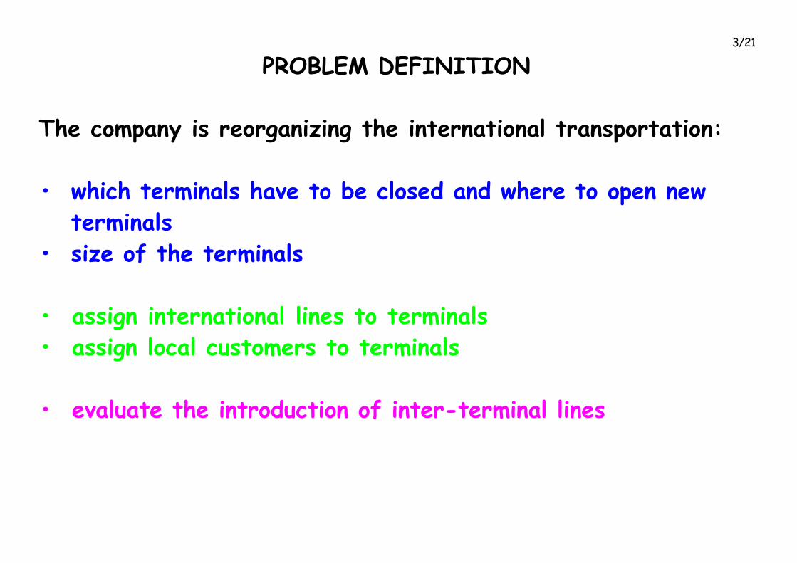
PROBLEM DEFINITION

The company is reorganizing the international transportation:

¥ which terminals have to be closed and where to open new

terminals

¥ size of the terminals

¥ assign international lines to terminals

¥ assign local customers to terminals

¥ evaluate the introduction of inter-terminal lines

4/21

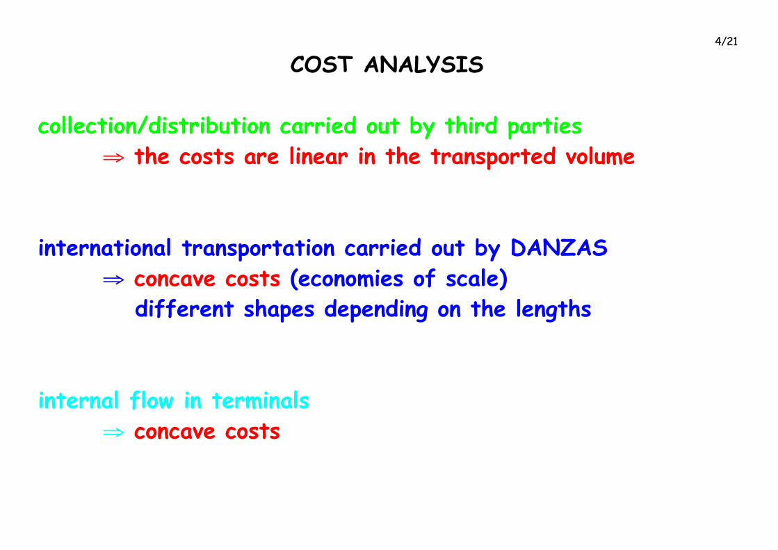
COST ANALYSIS

collection/distribution carried out by third parties

Þ the costs are linear in the transported volume

international transportation carried out by DANZAS

Þ concave costs (economies of scale)

different shapes depending on the lengths

internal flow in terminals

Þ concave costs

5/21

International transportation costs

y = 1.7325x0.6678

R2 = 0.928

0

2,000

4,000

6,000

8,000

10,000

12,000

0 50,000 100,000 150,000 200,000 250,000 300,000 350,000 400,000 450,000 500,000

Flow in Kg

cost

in

CH

F

6/21

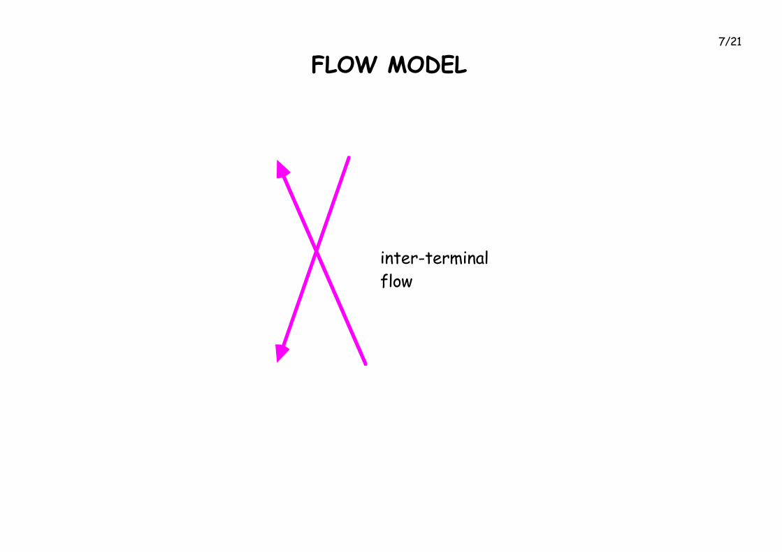
FLOW MODEL

terminal 1

terminal 2

domesticcustomers

international destinations

1 1'

2 2'

7/21

FLOW MODEL

terminal 1

terminal 2

domesticcustomers

international destinations

inter-terminalflow

8/21

FLOW MODEL

commodities jk (domestic origin j, international destination k)

dÊ

jk = volume of goods to be transported from j to k

xjk

jh = amount of flow of commodity jk going to terminal h

xjk

hh' = amount of flow of commodity jk inside terminal h

xjk

h'k = amount of flow of commodity jk going to destination k

from terminal h

zÊh = 1 if terminal h is activated, 0 otherwise

9/21

FLOW MODEL

min åjÊå

hÊf

jh

c (åkÊx

jk

jh) + åhÊ f

h

m(åjk

Êxjk

hh',zÊh) + å

kÊå

hÊf

hk

i (åjÊx

jk

h'k)

Ejkxjk = djk for each commodity jk [flow conservation]

xjk

hh' £ uhzh for each commodity jk and terminal h

[design]

Ejk is the node/arc incidence matrix related to commodity jk

djk is the demand vector

uh is an upper bound of the flow passing by terminal h

10/21

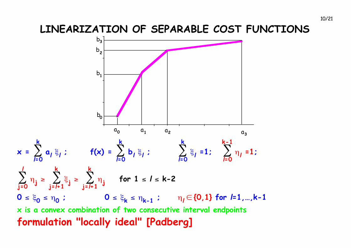
LINEARIZATION OF SEPARABLE COST FUNCTIONS

a0 a1 a2 a3

b0

b3

b1

b2

x = ål=0

k

Êal xl ; f(x) = ål=0

k

Êbl xl ; ål=0

k

Êxl =1; ål=0

k-1

Êhl =1;

åj=0

l

Êhj ³ åj=l+1

k

Êxj ³ åj=l+1

k

Êhj for 1 £ l £ k-2

0 £ x0 £ h0 ; 0 £ xk £ hk-1 ; hl Î {0,1} for l=1,É,k-1

x is a convex combination of two consecutive interval endpoints

formulation "locally ideal" [Padberg]

11/21

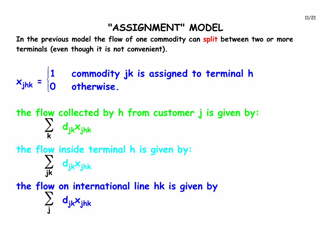
"ASSIGNMENT" MODELIn the previous model the flow of one commodity can split between two or more

terminals (even though it is not convenient).

xjhk = îïíïì1 commodityÊjkÊisÊassignedÊtoÊterminalÊh

0 otherwise.

the flow collected by h from customer j is given by:

åkÊ djkxjhk

the flow inside terminal h is given by:

åjk

Ê djkxjhk

the flow on international line hk is given by

åjÊ djkxjhk

12/21

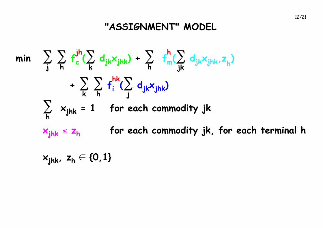
"ASSIGNMENT" MODEL

min åjÊå

hÊf

jh

c (åkÊdjkxjhk) + å

hÊ f

h

m(åjk

Êdjkxjhk,zÊh)

+ åkÊå

hÊf

hk

i (åjÊdjkxjhk)

åhÊ xjhk = 1 for each commodity jk

xjhk £ zh for each commodity jk, for each terminal h

xjhk, zh Î {0,1}

13/21

"ASSIGNMENT" MODEL

Inter-terminal flows

xjhrk = îïíïì1 commodityÊjkÊusesÊterminalsÊhÊandÊrÊinÊtheÊorder

0 otherwise.

the constraints are modified accordingly

14/21

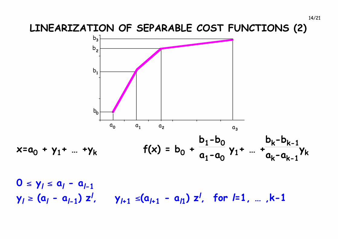
LINEARIZATION OF SEPARABLE COST FUNCTIONS (2)

a0 a1 a2 a3

b0

b3

b1

b2

x=a0 + y1+ É +yk f(x) = b0 + b1-b0

a1-a0 y1+ É +

bk-bk-1

ak-ak-1yk

0 £ yl £ al - al-1

yl ³ (al - al-1) zl, yl+1 £(al+1 - al1) z

l, for l=1, É ,k-1

15/21

a0 a1 a2 a3

b0

b3

b1

b2

x

y1z

0=1

1 ³ z1 ³z2 ³ É ³ zk-1 ³0

Also this formulation is "locally ideal" [Padberg]

16/21

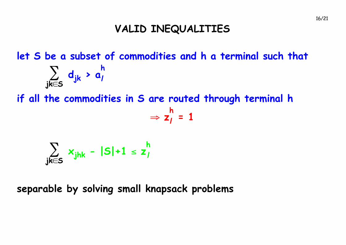
VALID INEQUALITIES

let S be a subset of commodities and h a terminal such that

åjkÎS

Ê djk > ah

l

if all the commodities in S are routed through terminal h

Þ zh

l = 1

åjkÎS

Ê xjhk - |S|+1 £ zh

l

separable by solving small knapsack problems

17/21

COMPUTATIONAL RESULTS

4 instances derived from real data provided by DANZAS

domestic areas / terminals / international destinations

"assignment" model "flow" model

# var. # constr. # var. # constr.

3 / 2 / 2 37 110 26 21

6 / 4 / 5 206 241 624 540

15 / 10 / 10 1930 2214 2036 920

60 / 9 / 10 1930 2190 1084 734

18/21

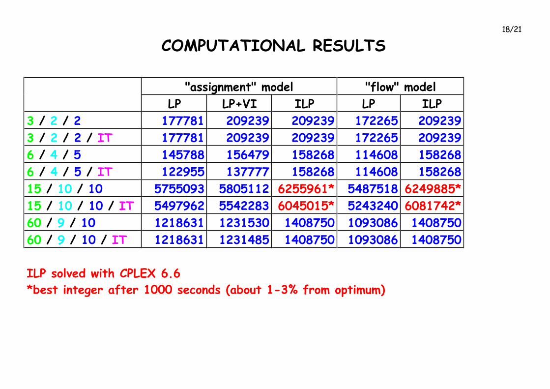
COMPUTATIONAL RESULTS

"assignment" model "flow" model

LP LP+VI ILP LP ILP

3 / 2 / 2 177781 209239 209239 172265 209239

3 / 2 / 2 / IT 177781 209239 209239 172265 209239

6 / 4 / 5 145788 156479 158268 114608 158268

6 / 4 / 5 / IT 122955 137777 158268 114608 158268

15 / 10 / 10 5755093 5805112 6255961* 5487518 6249885*

15 / 10 / 10 / IT 5497962 5542283 6045015* 5243240 6081742*

60 / 9 / 10 1218631 1231530 1408750 1093086 1408750

60 / 9 / 10 / IT 1218631 1231485 1408750 1093086 1408750

ILP solved with CPLEX 6.6

*best integer after 1000 seconds (about 1-3% from optimum)

19/21

COMPUTATIONAL RESULTS

"assignment" model "flow" model

LP LP+VI LP

3 / 2 / 2 15.0% 0.0% 17.7%3 / 2 / 2 / IT 15.0% 0.0% 17.7%6 / 4 / 5 7.9% 1.1% 27.6%6 / 4 / 5 / IT 22.3% 12.9% 27.6%15 / 10 / 10 8.0% 7.2% 12.2%15 / 10 / 10 / IT 9.0% 8.3% 13.8%60 / 9 / 10 13.5% 12.6% 22.4%60 / 9 / 10 / IT 13.5% 12.6% 22.4%

20/21

Comparison with the best solution obtained with 9 open

terminals

optimal solution 9 terminals gap

60 / 9 / 10 1408750 1572002 11.6%

21/21

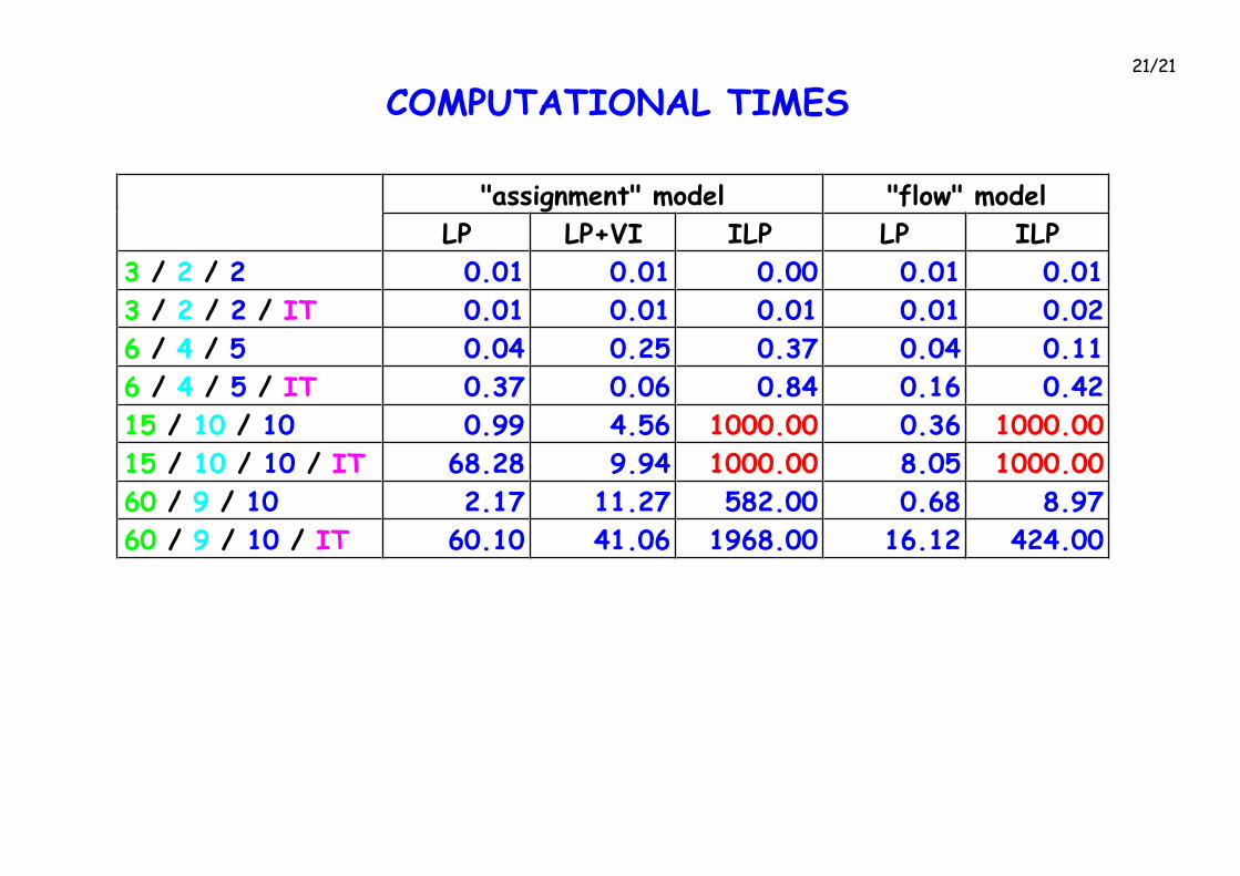
COMPUTATIONAL TIMES

"assignment" model "flow" model

LP LP+VI ILP LP ILP

3 / 2 / 2 0.01 0.01 0.00 0.01 0.01

3 / 2 / 2 / IT 0.01 0.01 0.01 0.01 0.02

6 / 4 / 5 0.04 0.25 0.37 0.04 0.11

6 / 4 / 5 / IT 0.37 0.06 0.84 0.16 0.42

15 / 10 / 10 0.99 4.56 1000.00 0.36 1000.00

15 / 10 / 10 / IT 68.28 9.94 1000.00 8.05 1000.00

60 / 9 / 10 2.17 11.27 582.00 0.68 8.97

60 / 9 / 10 / IT 60.10 41.06 1968.00 16.12 424.00