Improving Transient Stability of Power Systems by using passivity-based Nonlinear STATCOM

Controller

A THESIS SUBMITTED IN PARTIAL FULFILLMENT OF THE

REQUIREMENTS FOR THE DEGREE OF

Master of Technology

In

Power Control and Drives

By

D. Raghu Rama Reddy

Department of Electrical Engineering

National Institute of Technology

Rourkela

2007

Improving Transient Stability of Power Systems by using passivity-based Nonlinear STATCOM

Controller

A THESIS SUBMITTED IN PARTIAL FULFILLMENT OF THE

REQUIREMENTS FOR THE DEGREE OF

Master of Technology

In

Power Control and Drives

By

D.Raghu Rama Reddy

Under the Guidance of

Prof. P.C. Panda

Department of Electrical Engineering

National Institute of Technology

Rourkela

2007

National Institute of Technology

Rourkela

CERTIFICATE

This is to certify that the thesis entitled, “Improving Transient Stability of Power Systems

by using Passivity-bassed Nonlinear STATCOM Controller ” submitted by Sri D. Raghu

Rama Reddy” in partial fulfillment of the requirements for the award of MASTER of

Technology Degree in Electrical Engineering with specialization in “Power Control and

Drives” at the National Institute of Technology, Rourkela (Deemed University) is an

authentic work carried out by him/her under my/our supervision and guidance.

To the best of my knowledge, the matter embodied in the thesis has not been submitted to any

other University/ Institute for the award of any degree or diploma.

Date: Prof. P.C.Panda

Dept.of Electrical Engg. National Institute of Technology

Rourkela - 769008

ACKNOWLEDGEMENT

My sincere thanks to my guide Prof.P.C.Panda for his able guidance and constant support. I

extend my thanks to our HOD, Dr. P.K.Nanda for his valuable advices, and to our PG-

Coordinator Dr. A.K.Panda for his cooperation and encouragement, I extend my sincere

thanks to all faculty and non-faculty members of the Department for their help directly or

indirectly, during the course of my thesis work. I am also thankful to my batch mates for their

kind cooperation during the course of thesis work.

Raghu Rama Reddy.D

CONTENTS Page No.

Abstract i

List of Figures ii

List of Tables ii

1. INTRODUCTION 1

1.1 Background 3

1.1.1 Need For Dynamic voltage compensation 3

1.1.2 Solution for Dynamic Voltage compensation 4

1.1.3 STATCOM Technology in brief 5

1.1.4 STACOM Control strategies 6

1.2 Objective 8

1.3 Thesis Outline 9

2. INTRODUCTION TO PASSIVITY-BASED CONTROL OF

EULER-LAGRANGE SYSTEMS

2.1 Why is the theory needed? 10

2.2 EL systems and passive EL systems 10

2.3 Passivity Based Control 10

2.4 The Euler- Lagrange equations 14

2.4.1 Assumptions and properties 14

2.4.2 External forces 15

2.4.3 Dissipativity and passivity 15

2.4.4 Stability properties 16

3. EL MODEL OF THE STATCOM 17

3.1 EL Model in a-b-c Reference Frame 17

3.2 EL Model in d-q Reference Frame 21

4. NONLINEAR STATCOM CONTROLLER DESIGN

4.1 Control Design 24

5. SIMULATION RESULTS AND DISCUSSION

5.1 PSCAD simulation results 29

5.2 Discussions 34

6. CONCLUSION AND SCOPE FOR FUTURE WORK

6.1 Conclusion 35

6.2 Scope for future work 35

REFERENCES 36

ABSTRACT

This report presents a novel nonlinear control scheme for designing Static Synchronous

Compensators (STATCOM).A passivity-based approach is proposed for designing robust

nonlinear STATCOM controller. The mathematical model of STATCOM will be represented

by a Euler-Lagrange (EL) system corresponding to a set of EL parameters. The STATCOM

modeled in the a–b–c reference frame are first shown to be EL systems whose EL parameters

are explicitly identified. The energy-dissipative properties of this model are fully retained

under the d-q axis transformation. By employing the Park’s transformation, the differential

geometry approach is used to investigate the power system dynamics with considering

STATCOM under the synchronous d-q frame. Based on the transformed d-q EL model,

passivity-based controllers are then synthesized using the technique of damping injection.

Two possible passivity-based feedback designs are discussed, leading to a feasible dynamic

current-loop controller. Motivated from the usual power electronics control schemes, the

internal dc-bus voltage dynamics are regulated via an outer loop proportional plus integral

(PI) controller cascaded to the d-axis current loop. The STATCOM controller based on

passivity is obtained with a feedback control law from linear system models. The STATCOM

controlled by the proposed passivity-based current control scheme with outer loop PI

compensation has the features of enhanced robustness under model uncertainties, decoupled

current-loop dynamics, guaranteed zero steady-state error, and asymptotic rejection of

constant load disturbance. Digital computer simulation for a large operation point variations

have been studied the STATCOM controller design. For analysis of the system performance,

the PSCAD/EMTDC programme was applied. Simulation results show that the proposed

STATCOM controller can effectively enhance transient stability of the power system even in

the presence of large operation point variations.

i

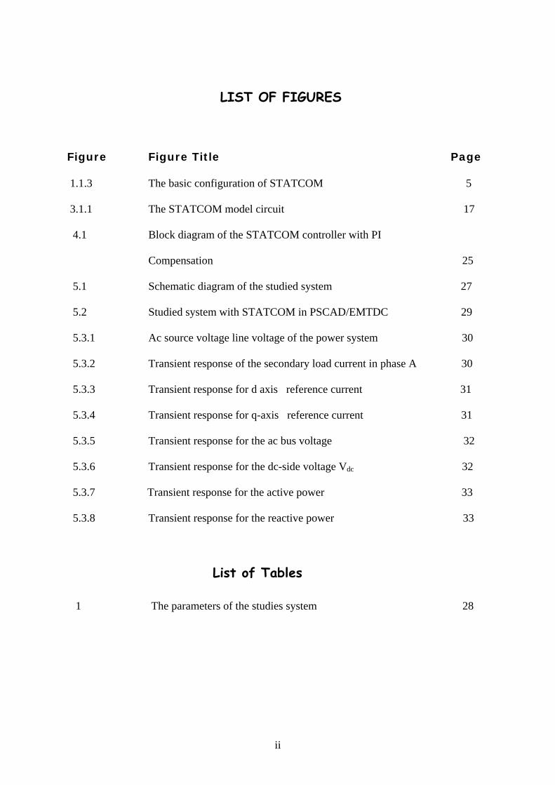
LIST OF FIGURES

Figure Figure Title Page

1.1.3 The basic configuration of STATCOM 5

3.1.1 The STATCOM model circuit 17

4.1 Block diagram of the STATCOM controller with PI

Compensation 25

5.1 Schematic diagram of the studied system 27

5.2 Studied system with STATCOM in PSCAD/EMTDC 29

5.3.1 Ac source voltage line voltage of the power system 30

5.3.2 Transient response of the secondary load current in phase A 30

5.3.3 Transient response for d axis reference current 31

5.3.4 Transient response for q-axis reference current 31

5.3.5 Transient response for the ac bus voltage 32

5.3.6 Transient response for the dc-side voltage Vdc 32

5.3.7 Transient response for the active power 33

5.3.8 Transient response for the reactive power 33

List of Tables

1 The parameters of the studies system 28

ii

INTRODUCTION

Background

Objective

Thesis Outline

INTRODUCTION

Recently, Flexible Alternative Current Transmission System (FACTS) controllers

have been proposed to enhance the transient or dynamic stability of power systems. During

the last decade, a number of control devices under the term FACTS technology have been

proposed and implemented. Among all FACTS devices, static synchronous compensators

(STATCOM) plays much more important role in reactive power compensation and voltage

support because of its attractive steady state performance and operating characteristics. The

fundamental principle of a STATCOM installed in a power system is the generation ac

voltage source by a voltage source inverter (VSI) connected to a dc capacitor. The active and

reactive power transfer between the power system and the STATCOM is caused by the

voltage difference across this reactance.

The basic function of the STATCOM is for the line voltage control, which is

implemented by an ac voltage controller in the STATCOM by regulating the reactive power

exchange between the STATCOM and power system. A second controller installed in the

STATCOM is the dc voltage controller, which regulates the dc voltage across the dc

capacitor of the STATCOM. In conventional control schemes, both the voltage regulators are

proportional integral (PI) type cascaded controllers. Recently, a linear multivariable

controller approach has been used for the STATCOM controller design for better

performance. However, since the complete model of STATCOM is highly nonlinear, the

linear approach obviously dose not lead to better dynamic decoupling.

The dynamical equations of the STATCOM is of nonlinear nature due to the

multiplication of the state variables by the control inputs a purely nonlinear approach without

ignoring these nonlinearities would be preferable for achieving non local stability or tracking

property. The recently developed passivity-based control methodology provides a viable

approach to do this job. Successful implementations of this type of control design have been

reported in various industrial applications [1]-[3]. Specifically, for control of induction

motors, robot arms, and switching power converters, it has been shown how to beneficially

incorporate the structural as well as energy properties of the Euler–Lagrange (EL) systems in

the controller synthesis. Enhanced robustness and simplified realization in controller

implementation are achieved as compared to the commonly used feedback linearizing law

due to the avoidance of exact cancellation of system nonlinearities. These attractive features

are resulted from the identification of “workless forces” terms appearing in the EL model. As

these workless forces have no effect on the energy balance equation and do not affect the

stability properties, there is no need to cancel them in the feed forward part of the control

1

law. The approach in designing a passivity-based controller can be summarized in the

following two steps. First, model the plant by EL formulation in which the system’s energy-

dissipative properties are exploited via identification of the Lagrangian and workless force.

Second, based on the EL description, the passivity-based control law is derived as a result to

reshape the system’s natural energy and add the required damping such that desired control

objectives are achieved.

In this paper, as an attempt to apply the passivity-based framework for the PWM

three-phase ac/dc boost converter, we first derive the EL dynamic expression of the three-

phase PWM rectifier. It is shown that a set of EL parameters can be identified to yield

corresponding EL structure and establish the passivity properties of the PWM converter in

both a–b–c and d–q reference frames [4]. The results also reveal that the three-phase boost

ac/dc converter is an under actuated EL system and a dynamic passivity-based controller is

synthesized from injecting required damping. The synthesis of the passivity-based controller

is carried out from two aspects. To accomplish dc-bus voltage regulation, a scheme (denoted

voltage control) that directly regulates output voltage is investigated. The resulting zero

dynamics are found to be unstable, indicating that this approach is not feasible. For this

reason, we proceed to adopt an indirect scheme (denoted current control) which performs dc-

bus voltage control through regulating input d-q axis line currents. Interestingly, similar

situations also appear in the passivity-based stabilization of dc-to-dc boost converters. This is

due to both these two types of converters, as output variables expressed in terms of dc output

voltage exhibit no minimum phase feature and the passivity-based controller realizes a partial

inversion of the system.

In the current control scheme, the output voltage on the dc side will be regulated to

the desired level indirectly once d–axis line current tracking is achieved. As an accurate d-

axis current command must be pre calculated using the system parameters and load

resistance, this kind of indirect output dc voltage control is very sensitive to model

uncertainties. A proportional plus integral (PI) controller is cascaded to the d-axis current

loop for robust tracking of constant dc-voltage reference. In view of the overall system

configuration, it is found that the proposed dc-bus voltage controller is nothing but the outer

loop controller. Although this kind of configuration is common, it provides an effective

means for improving the performance of passivity based control systems where the state

vector of the internal dynamics contains some desired control variables. This modified

control scheme will be termed passivity-based current control with outer loop PI

compensation in the following paragraphs. For example, for the dc-to-dc converter in [5] the

2

internal dynamics were not controlled so that the states of the internal dynamics evolved with

convergent rates determined by the inherent time constants.

As the dc-bus voltage dynamics contain a nonlinear input mapping, we establish the

global regulation of the outer loop control system under the perfect tracking of inner current

loops by applying the results of Desoer and Lin [6]. The proposed passivity-based schemes

are then realized in the laboratory via a personal computer with data acquisition boards. A

1.5-kVA prototype PWM ac/dc converter using insulated gate bipolar transistor (IGBT)

power switches is built and experiments are conducted to test the performance of the

proposed controllers. For the purpose of comparison, the responses of the passivity based

current control scheme, passivity-based current control with outer loop PI compensation

scheme, and linear PI control scheme of [7] are provided. This paper is organized as follows.

Section II presents the derivation of the EL models of the three-phase PWM boost converter

in both a–b–c and d–q reference frames. Section III describes the synthesis of passivity-based

voltage and current controllers, directly or indirectly achieving dc-bus voltage regulation,

respectively. The outer loop PI control of the internal dc-bus voltage dynamics is discussed in

Section IV. Experimental results are documented in Section V. A conclusion is finally given

in Section VI.

The use of the passivity-based approach to design nonlinear controllers of power

converters has been proposed in [8]. In this paper, a passivity-based approach is proposed for

designing robust nonlinear STATCOM controller. Mathematically, the STATCOM can be

represented by a Euler-Lagrange (EL) system corresponding to a set of EL parameters.

Therefore, a STATCOM controller based on passivity consideration is obtained with a

feedback control law from linear system models. Simulation results show that the proposed

STATCOM controller can effectively enhance transient stability of the power system even in

the presence of large operation point variations.

1.1 BACK GROUND

1.1.1 Need for Dynamic voltage compensation

High Intensity Discharge (HID) lamps used for industrial illumination get extinguished at

voltage dips of 20%. Also, critical industrial equipment like Programmable Logic Controllers

(PLCs) and Adjustable Speed Drives (ASDs) are adversely affected by voltage dips of about

10%. The starting current of the induction motor being 6 times its rated current it provides the

sag mitigation. Voltage sag has been defined as a reduction in the voltage magnitude from its

nominal value for a duration ranging from a few milli seconds to one minute.

3

1.1.2 Solution for Dynamic Voltage compensation

Solution approaches to the voltage disturbance problem, using active devices, can involve

either i) a series injection of voltage, or ii) a shunt injection of reactive current. The Static

Var Compensator (SVC) and the STATCOM are the available shunt compensation devices. The speed of devices for power quality improvement (FACTS), which was made

possible by the evolution of power electronics components, allows for the solving of

problems such as voltage stability, transient improvement, oscillations damping and

improvement of the lines performance. The term FACTS describes a wide range of

controllers, many of which incorporate large power electronic converters, that can increase

the flexibility of power systems making them more controllable. Some of these are already

well established while some are still in the research or development stage.

In general, FACTS devices possess the following technological attributes:

• Provide dynamic reactive power support and voltage control.

• Reduce the need for construction of new transmission lines, capacitors, reactors, etc

which

– Mitigate environmental and regulatory concerns.

– Improve aesthetics by reducing the need for construction of new facilities such as

transmission lines.

• Improve system stability.

• Control real and reactive power flow.

• Mitigate potential Sub-Synchronous Resonance problems.

To determine which FACTS device would be the most beneficial

• Thyristor Controlled Series Capacitor (TCSC)

• Thyristor Controlled Phase Angle regulator (TCPAR)

• Static Compensator (STATCOM)

• Unified Power Flow Controller (UPFC)

While TCSC provides dynamic control of the series compensated lines, which could increase

transfer capability. A TCPAR, is equivalent to a mechanically phase shifting transformer but

unlike a UPFC it does not provide controlled reactive power generation. Since a STATCOM

mainly provides dynamic reactive power to the Transmission system but as it does not

directly control the flow of real power on a transmission line. A UPFC, by providing a

combination of real and reactive power control, appeared to be the most useful FACTS

4

device. It could potentially control power flow on the line, reduce the number of lines that

can be overloaded, and potentially provide dynamic reactive power control during

contingencies.

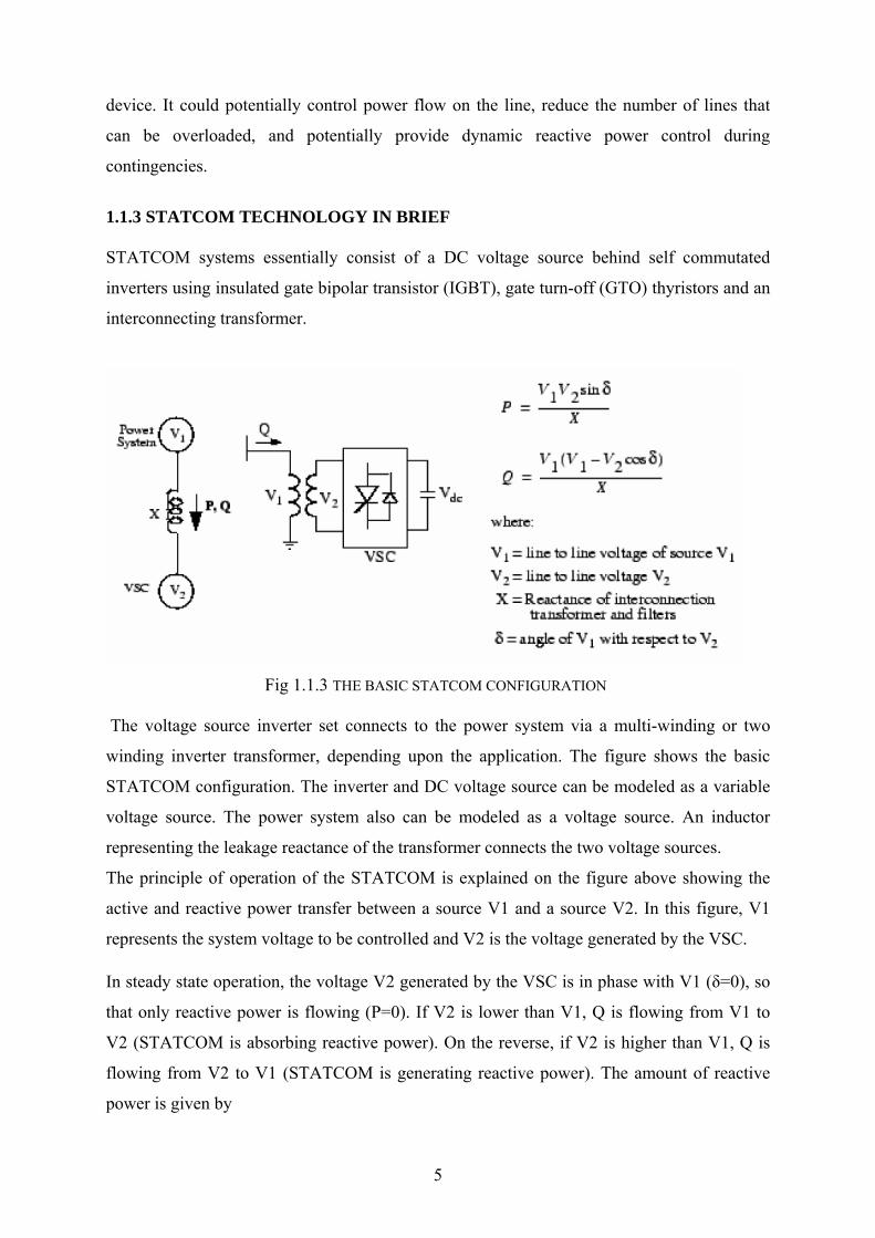
1.1.3 STATCOM TECHNOLOGY IN BRIEF STATCOM systems essentially consist of a DC voltage source behind self commutated

inverters using insulated gate bipolar transistor (IGBT), gate turn-off (GTO) thyristors and an

interconnecting transformer.

Fig 1.1.3 THE BASIC STATCOM CONFIGURATION The voltage source inverter set connects to the power system via a multi-winding or two

winding inverter transformer, depending upon the application. The figure shows the basic

STATCOM configuration. The inverter and DC voltage source can be modeled as a variable

voltage source. The power system also can be modeled as a voltage source. An inductor

representing the leakage reactance of the transformer connects the two voltage sources.

The principle of operation of the STATCOM is explained on the figure above showing the

active and reactive power transfer between a source V1 and a source V2. In this figure, V1

represents the system voltage to be controlled and V2 is the voltage generated by the VSC.

In steady state operation, the voltage V2 generated by the VSC is in phase with V1 (δ=0), so

that only reactive power is flowing (P=0). If V2 is lower than V1, Q is flowing from V1 to

V2 (STATCOM is absorbing reactive power). On the reverse, if V2 is higher than V1, Q is

flowing from V2 to V1 (STATCOM is generating reactive power). The amount of reactive

power is given by

5

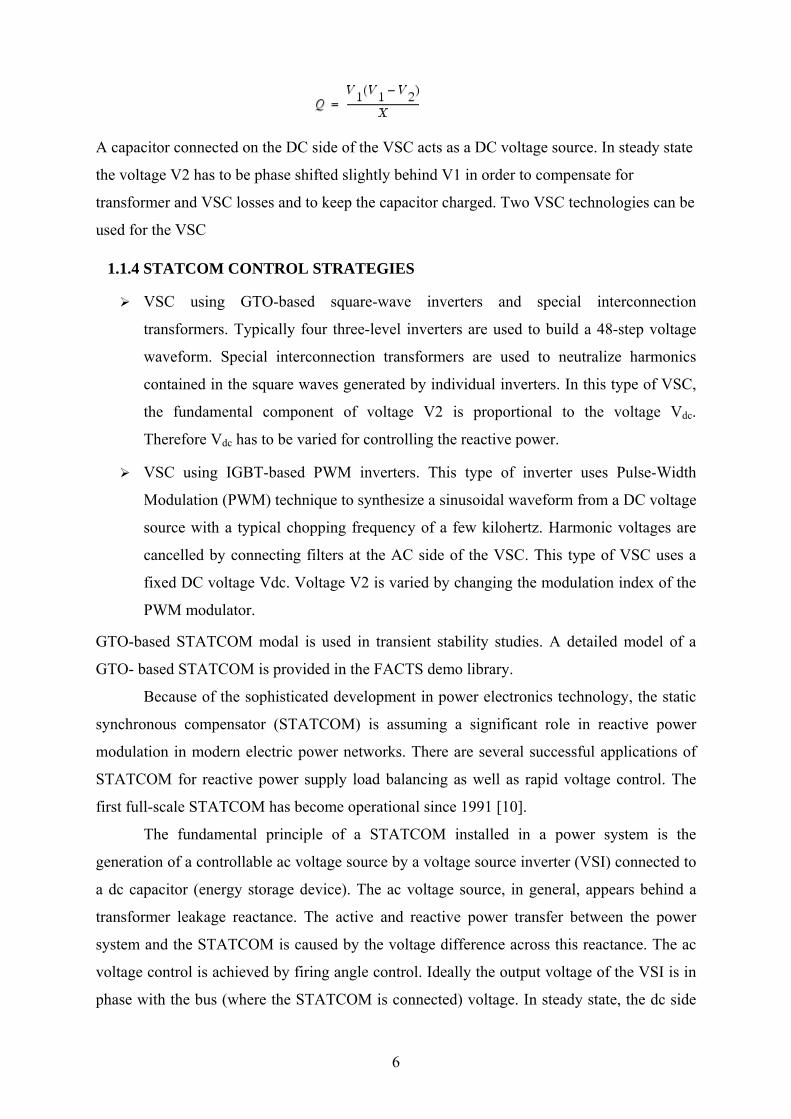
A capacitor connected on the DC side of the VSC acts as a DC voltage source. In steady state

the voltage V2 has to be phase shifted slightly behind V1 in order to compensate for

transformer and VSC losses and to keep the capacitor charged. Two VSC technologies can be

used for the VSC

1.1.4 STATCOM CONTROL STRATEGIES

VSC using GTO-based square-wave inverters and special interconnection

transformers. Typically four three-level inverters are used to build a 48-step voltage

waveform. Special interconnection transformers are used to neutralize harmonics

contained in the square waves generated by individual inverters. In this type of VSC,

the fundamental component of voltage V2 is proportional to the voltage Vdc.

Therefore Vdc has to be varied for controlling the reactive power.

VSC using IGBT-based PWM inverters. This type of inverter uses Pulse-Width

Modulation (PWM) technique to synthesize a sinusoidal waveform from a DC voltage

source with a typical chopping frequency of a few kilohertz. Harmonic voltages are

cancelled by connecting filters at the AC side of the VSC. This type of VSC uses a

fixed DC voltage Vdc. Voltage V2 is varied by changing the modulation index of the

PWM modulator.

GTO-based STATCOM modal is used in transient stability studies. A detailed model of a

GTO- based STATCOM is provided in the FACTS demo library.

Because of the sophisticated development in power electronics technology, the static

synchronous compensator (STATCOM) is assuming a significant role in reactive power

modulation in modern electric power networks. There are several successful applications of

STATCOM for reactive power supply load balancing as well as rapid voltage control. The

first full-scale STATCOM has become operational since 1991 [10].

The fundamental principle of a STATCOM installed in a power system is the

generation of a controllable ac voltage source by a voltage source inverter (VSI) connected to

a dc capacitor (energy storage device). The ac voltage source, in general, appears behind a

transformer leakage reactance. The active and reactive power transfer between the power

system and the STATCOM is caused by the voltage difference across this reactance. The ac

voltage control is achieved by firing angle control. Ideally the output voltage of the VSI is in

phase with the bus (where the STATCOM is connected) voltage. In steady state, the dc side

6

capacitance is maintained at a fixed voltage and there is no real power exchange, except for

losses.

The STATCOM differs from other reactive power generating devices (such as

Capacitors, Static Var Compensators etc.) in the sense that the ability for energy storage is

not a rigid necessity but is only required for system unbalance or harmonic absorption. As a

consequence, the not-a-so-strict requirement for large energy storage device makes

STATCOM more robust and it also enhances the response speed.

Basically, there are two control objectives implemented in the STATCOM. One is the

ac voltage regulation of the power system at the bus where the STATCOM is connected and

the other is dc voltage control across the capacitor inside the STATCOM. It is widely known

that shunt reactive power injection can be used to control the bus voltage. In conventional

control scheme, there are two voltage regulators designed for these purposes: ac voltage

regulator for bus voltage control and dc voltage regulator for capacitor voltage control. In the

simplest strategy, both the voltage regulators are proportional integral (PI) type cascaded

controllers [11,12] The modeling and control design is usually carried out in the synchronous

d -/q frame, as it is quite standard. Thus, the shunt current is split into d-axis and q-axis

components. The reference values for these currents are obtained by separate PI regulators

from dc voltage and ac-bus voltage errors, respectively. Then, subsequently, these reference

currents are regulated by another set of PI regulators whose outputs are the d-axis and q-axis

control voltages for the STATCOM. Although, this cascade control structure yields good

performance, it is not very much effective for all operating conditions because, in general,

one chosen set of PI-gains may not be suitable for all operating points. Moreover, it really

becomes a hard task to choose the PI gains for the four PI regulators occurring in the cascade

structure because of the inherent coupling between the d-axis and q-axis variables. Recently,

a linear multivariable controller approach has been used for the control design for better

performance. However, since the complete model is highly nonlinear, the linear approach

obviously does not lead to better dynamic decoupling. a nonlinear multivariable control

technique for STATCOM using feedback linearization approach. The feedback linearization

technique is based on the idea of canceling the nonlinearities of the system and imposing a

desired linear dynamics to control the system.

The problem of voltage compensation, using a STATCOM, has been addressed in

literature. In, a small-signal analysis of the system was performed with a transmission line,

which was modeled as a network. Presence of right-half plane zeros in the transfer function

was detected and an integral controller, cascaded with a second-order notch-filter was

7

proposed. An exclusively experimental study of voltage sag mitigation, using reactive power

injection, can be found in. Here, a distribution line was considered and modeled as a series

reactance. It should be noted that PQ issues are mostly relevant in the distribution system and

distribution feeders, of length less than 80 km, can be correctly modeled as a series

impedance.

The basic function of the STATCOM is for the line voltage control, which is

implemented by an ac voltage controller in the STATCOM by regulating the reactive power

exchange between the STATCOM and power system. A second controller installed in the

STATCOM is the dc voltage controller, which regulates the dc voltage across the dc

capacitor of the STATCOM. In conventional control schemes, both the voltage regulators are

proportional integral (PI) type cascaded controllers. Recently, a linear multivariable

controller approach has been used for the STATCOM controller design for better

performance. However, since the complete model of STATCOM is highly nonlinear, the

linear approach obviously dose not lead to better dynamic decoupling.

To overcome this limitation, several nonlinear control schemes have been proposed to

design the STATCOM controller. The feedback linearization approach, based on the idea of

canceling the nonlinearities of the system and imposing a desired linear dynamics to control

system, is presented in. The dissipativity-based design, relies on a frequency domain

modeling of a system dynamic using positive sequence and negative sequence dynamic

components, was applied successfully in.

The use of the passivity-based approach to design nonlinear controllers of power

converters has been proposed in. In this paper, a passivity-based approach is proposed for

designing robust nonlinear STATCOM controller. Mathematically, the STATCOM can be

represented by a Euler-Lagrange (EL) system corresponding to a set of EL parameters.

Therefore, a STATCOM controller based on passivity consideration is obtained with a

feedback control law from linear system models. Simulation results show that the proposed

STATCOM controller can effectively enhance transient stability of the power system even in

the presence of large operation point variations.

1.2. OBJECTIVE

In modern electrical distribution power systems there has been a sudden increase of single

phase and three-phase linear and non-linear loads. These non-linear loads employ solid state

power conversion and draw non-sinusoidal currents from AC mains and cause harmonics and

reactive power burden, and excessive neutral currents that result in pollution of power

8

systems. They also result in lower efficiency. Static Synchronous Compensators have been

developed to overcome these problems. STATCOM based on voltage controlled PWM

converters are seen as viable solution. The techniques that are used to generate desired

compensating reactive current or capacitive are based on instantaneous extraction of

compensating commands from the distorted currents or voltage signals in time domain. The

complete model of STATCOM is highly nonlinear, the linear approach obviously dose not

lead to better dynamic decoupling.

In this work a passivity-based approach is proposed for designing robust nonlinear

STATCOM controller Therefore, a STATCOM controller based on passivity consideration is

obtained with a feedback control law from linear system model can effectively enhance

transient stability of the power system even in the presence of large operation point

variations.

1.3 THESIS OUTLINE

The body of this thesis consists of the following five chapters including first chapter:

In chapter 2 the basic theory for passive EL systems is presented. We also present

stability theory for passive EL systems.

In chapter 3 described EL model of the STATCOM in a-d-c reference frame and d-q

reference frame.

In chapter 4 gives the control strategy for STATCOM concerns with the control of

ac and dc bus voltage on both sides of STATCOM.

In chapter 5 simulation results are put and discussed in detail with PI controller to

regulates the d-q axis current commands.

In chapter 6 deals the deals the conclusion and scope for future work.

9

INTRODUCTION TO PASSIVITY-BASED CONTROL OF EULER-LAGRANGE SYSTEMS Why is the theory needed?

EL systems and passive EL systems

Passivity Based Control

The Euler- Lagrange equations

2.1 Why is the theory needed? In classical control theory, linear models are considered. If the equations describing a system

are nonlinear, the system is linearised, which means that the nonlinear equations are

approximated with a linear system. This linear system is then used to determine the control

laws. The control laws derived from such an approach are sufficient in many practical

applications, but in some cases the linear approach is not sufficient. Therefore, a theory for

nonlinear control systems is needed. Unfortunately, nonlinear theory for general systems is

complicated and rarely useful in engineering applications.

To make nonlinear theory more useful, it is necessary to consider theory for classes

of systems with certain properties. The class of passive Euler-Lagrange (EL) systems consists

of systems that can be described by the EL equations and do not contain an internal energy

source. Examples of passive EL systems are passive electrical circuits, mechanical systems,

and robots.

With these special properties in mind, a more useful nonlinear control theory can be

presented and nonlinear controllers can be constructed from this theory.

2.2 EL systems and passive EL systems It is difficult to develop a general nonlinear control theory, because each type of nonlinear

system has its own characteristics. Therefore, theories for specialised types of systems are

potentially more useful in the analysis of nonlinear systems.

In this report we study a class of systems called Euler-Lagrange systems (EL

systems). An EL system is a system whose dynamics are described by the EL equations.

These equations are described in this chapter. We also define and investigate a special class

of EL systems called passive EL systems. Most of the theory in this report is connected to

that class of systems.

2.3 Passivity Based Control Consider the system ( , )x f x u=&

( )y h x=

Where and .This system is passive if there exists a C(0,0) 0f = (0) 0h = 1 positive semi-

definite function (storage function) such that ( )V x

10

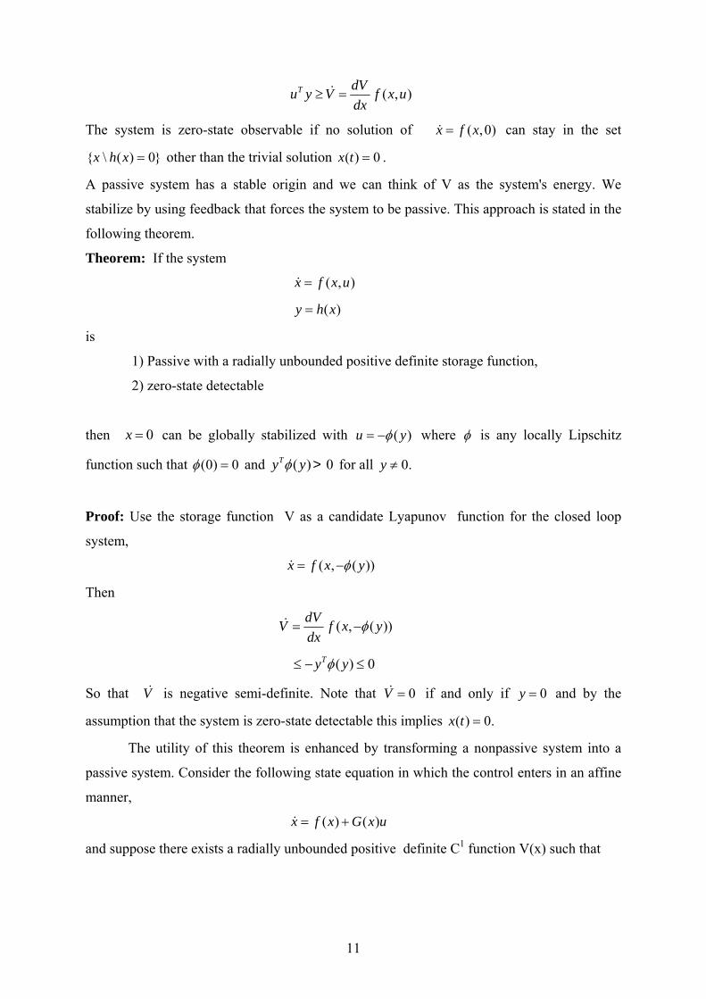
( , )T dVu y V f x udx

≥ =&

The system is zero-state observable if no solution of ( ,0)x f x=& can stay in the set

other than the trivial solution \ ( ) 0x h x = ( ) 0x t = .

A passive system has a stable origin and we can think of V as the system's energy. We

stabilize by using feedback that forces the system to be passive. This approach is stated in the

following theorem.

Theorem: If the system

( , )x f x u=&

( )y h x=

is

1) Passive with a radially unbounded positive definite storage function,

2) zero-state detectable

then can be globally stabilized with 0x = ( )u yφ= − where φ is any locally Lipschitz

function such that (0) 0φ = and for all ( ) 0Ty yφ > 0.y ≠

Proof: Use the storage function V as a candidate Lyapunov function for the closed loop

system,

( , ( ))x f x yφ= −&

Then

( , ( ))dVV f xdx

φ= −& y

( ) 0Ty yφ≤ − ≤

So that V is negative semi-definite. Note that & 0V =& if and only if and by the

assumption that the system is zero-state detectable this implies

0y =

( ) 0.x t =

The utility of this theorem is enhanced by transforming a nonpassive system into a

passive system. Consider the following state equation in which the control enters in an affine

manner,

( ) ( )x f x G x u= +&

and suppose there exists a radially unbounded positive definite C1 function V(x) such that

11

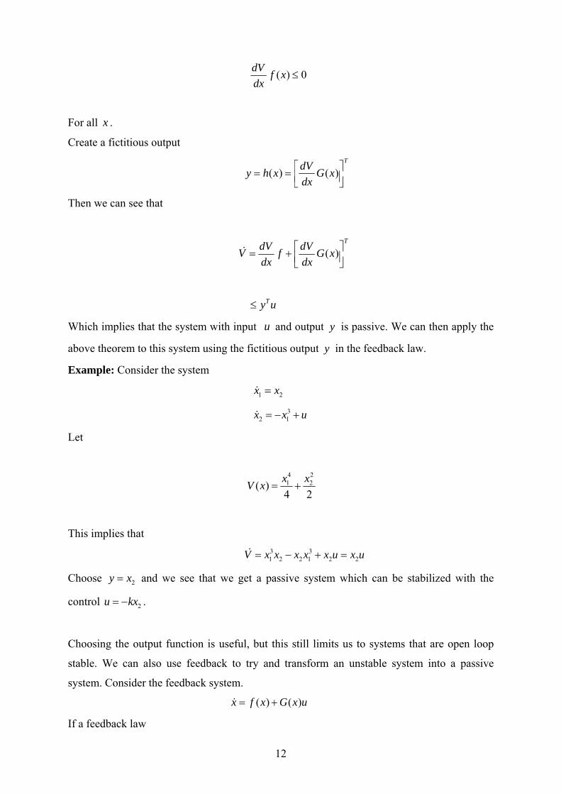
( ) 0dV f xdx

≤

For all . x

Create a fictitious output

( ) ( )TdVy h x G x

dx⎡ ⎤= = ⎢ ⎥⎣ ⎦

Then we can see that

( )TdV dVV f G x

dx dx⎡ ⎤= + ⎢ ⎥⎣ ⎦

&

Ty u≤

Which implies that the system with input and output is passive. We can then apply the

above theorem to this system using the fictitious output in the feedback law.

u y

y

Example: Consider the system

1 2x x=&

32 1x x u= − +&

Let

4 21 2( )4 2x xV x = +

This implies that

3 31 2 2 1 2 2V x x x x x u x u= − + =&

Choose and we see that we get a passive system which can be stabilized with the

control .

2y x=

2u kx= −

Choosing the output function is useful, but this still limits us to systems that are open loop

stable. We can also use feedback to try and transform an unstable system into a passive

system. Consider the feedback system.

( ) ( )x f x G x u= +&

If a feedback law

12

( ) ( )u x x uα β= +

exists and an output exists such that ( )h x y=

( ) ( ) ( ) ( ) ( )x f x G x x G x x uα β= + +&

( )y h x=

is passive and zero-state detectable, then we can use our preceding theorem. This is

sometimes referred to as feedback passivation. This can often be done for “Hamiltonian”

systems that arise in many mechanical applications.

Passivation of m link Robot: Consider the following equations of motion for a typical

kinematic system,

−

( ) ( , ) ( )u M q q C q q q Dq g q= + + +&& & & &

Consider the tracking problem that seeks to make re q q= − small. The tracking error

dynamics are

( ) ( , ) ( )M q e C q q e De g q u+ + + =&& & & &

We want to stabilize around and 0e =& 0e = . But this is not necessarily a stable equilibrium

point.

Let

( ) pu g q K e u= − +

Where pK is a positive definite symmetric matrix and is an additional control input.

Under this change of control variable, we get

u

( ) ( , ) pM q e C q q e De K e u+ + + +&& & & &

We now consider

1 1( )2 2

T TpV e M q e e K= +& e

as a storage function, then clearly

12

T T TpV e Me e Me e K e= + +& & && & & &

1 ( 2 )( )2

T T T Tp pe M C e e De e K e e u e K e= − − − + +&& & & & & & T

Te u≤ &

Defining the output as we see that the system with input u and output is passive

with V as the storage function. The role of the passifying feedback is to reshape

,y e= & y

( ) pg q K e−

13

the potential energy to 12

Tpe K e which has a unique minimum at 0e = . As a result of this

choice of passivating control, the storage function becomes the sum of kinetic energy and

reshaped potential energy with . 0u = ( ) 0y t = if and only if ( ) 0e t =& which implies that

and hence so this system is also zero-state detectable. ( ) 0pK e t = ( ) 0.e t =

So we’ve just shown that this mechanical system can be globally stabilizied by the

control ( ).u eφ= − && the choice of results in the actual control law. du K= − &e

d ( ) ( )p ru g q K q q K q= − − + &

which is a classical PD controller with a gravity compensation term.

2.4 The Euler- Lagrange equations

The Euler-Lagrange equations were originally used to describe the dynamics of mechanical

systems. They can be shown to be equivalent to Newton’s second law. The advantage of the

EL formulation is that the form of the EL equations is invariant, independently of what

coordinates that are used. The EL equations can also be used to describe the dynamics of

other physical systems, such as electrical systems. A derivation of the EL equations is beyond

the scope of this report.

We recall that a dynamical system with n degrees of freedom can be described by the

Euler-Lagrange equations.

( ) ( ), ,d L Lq q q q Qdt q q⎛ ⎞∂ ∂

− =⎜ ⎟∂ ∂⎝ ⎠& &

&

Where are generalized coordinates, Q are external forces, and q ( ),L q q& is the Lagrangian

function. The Lagrangian is defined as ( , ) ( , ) ( )L q q T q q V q= −& & , where

( , )T q q& is the kinetic energy function and is the potential energy function. Generalized

coordinates q are used.

( )V q

2.4.1 Assumptions and properties Assumption1 We assume that all kinetic energy functions are of the quadratic form

1( , ) ( )2

TT q q q D q q=& & &

Where is called the general inertia matrix. This matrix satisfies ( ) nXnD q ∈R

( ) ( ) 0,TD q D q= > i.e. the matrix is symmetric and positive definite.

14

Assumption 2 The inertia matrix D(q) is positive definite and symmetric, and is also

bounded from above and below, i.e. it satisfies the inequality

( )m Md I D q d I< <

where and md Md are constants.

Assumption 3 The potential energy function V (q) is radially unbounded, globally positive

definite, and has a unique minimum at q q= . It is also assumed that V (q) does not have any

other critical points, that is q q= is the only solution of 0dVdq

=

2.4.2 External forces

There are three different types of external forces that we consider in this report: Control input

forces, dissipation forces, and forces from the interaction between the system and its

environment (disturbance forces).

The control forces are assumed to enter the system linearly and can thus be described as Mu,

where M is a constant control matrix and u is the control vector, that is, a vector containing

all the control signals.

The dissipation forces are always of the form ( )dF qdq

−&

&, where is called the Rayleigh

dissipation function, which by definition satisfies

( )F q&

( ) 0T dFq qdq

≥& &&

Using these three forces, the external forces can be written as

( ) udFQ q Qdq ζ= + +&&

M

Where Qζ denotes the disturbance forces.

2.4.3 Dissipativity and passivity

The properties of dissipativity and passivity are very important in the analysis of EL

systems. The theory presented in this report is mostly based on passive systems. A passive

system is a system that can not store more energy than is supplied to it. In other words, a

passive system does not contain an energy source.

15

Dissipativity : An EL system is dissipative with respect to the supply if and only if

there exists a storage function H such that

( , )s u y

0

( ( )) ( (0)) ( ( ), ( )T

H x T H x s u t y t dt≤ + ∫

For all , all and all u 0T ≥ 0x

Passivity of EL systems: A system is passive if it is dissipative with supply rate

. Because the supplied energy is greater than or equal to the total energy H, the

passivity property can also be written as

( , ) Ts u y u y=

[ ] [ ]( ) ( ), ( ) (0). (0)u G u H q T q T H q q ≥ −& &

2.4.4 Stability properties

Here, we present some stability related properties for unforced EL systems, i.e. . To

make it easier to understand, we study stability for fully damped and under damped systems

separately.

0u =

Fully damped systems are more stable than under damped systems, and the stability

properties are simpler. If the system is not fully damped, global asymptotic stability can be

ensured if the inertia matrix has a certain block-diagonal structure. We consider

systems with partial damping, i.e. the generalised coordinates q can be partitioned in damped

coordinates and undamped coordinates . The indices c and p denote controller and

process, respectively. The reason for this notation is that a process can often be considered as

an under damped system and the controller a damped one.

( )D q

cq pq

The under actuated system imposes some limitations to the modified potential

function. The equilibrium of the potential function can only be modified in terms of actuated

coordinates which leads to that the closed loop system can only be globally stabilised at a

desired equilibrium point chosen in terms of actuated coordinates. These constraints are

clearly removed for the fully actuated system where it is possible to modify the potential

function in terms of all coordinates. The properties of the potential function and the

uniqueness of the equilibrium point.

16

EL MODEL OF THE STATCOM EL Model in a-b-c Reference Frame EL Model in d-q Reference Frame

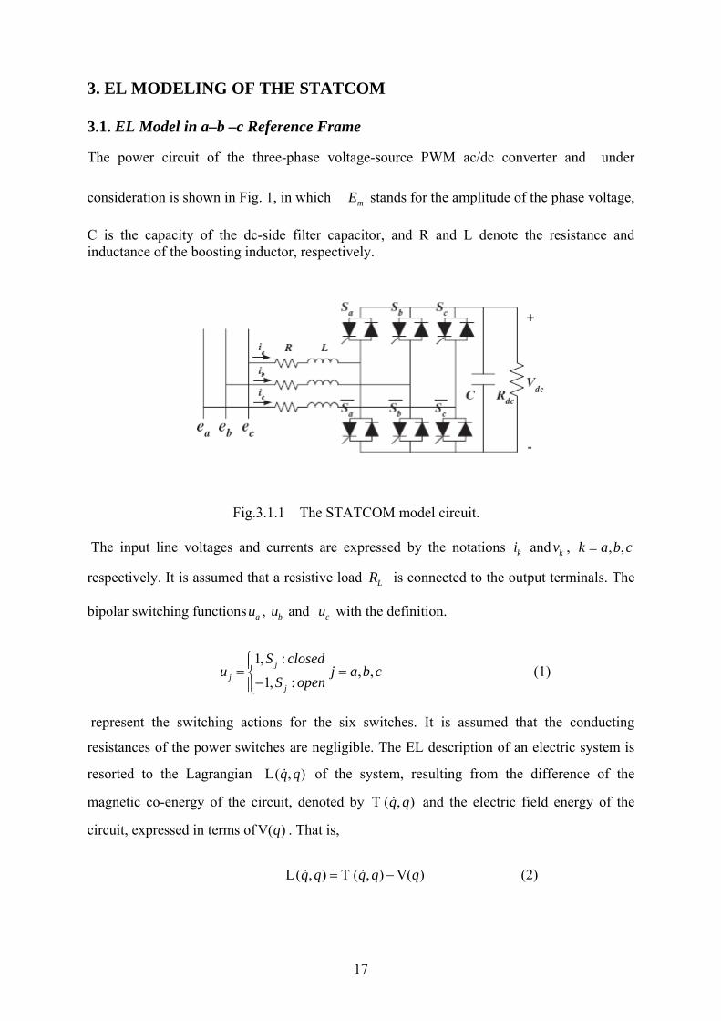
3. EL MODELING OF THE STATCOM 3.1. EL Model in a–b –c Reference Frame The power circuit of the three-phase voltage-source PWM ac/dc converter and under

consideration is shown in Fig. 1, in which stands for the amplitude of the phase voltage,

C is the capacity of the dc-side filter capacitor, and R and L denote the resistance and inductance of the boosting inductor, respectively.

mE

Fig.3.1.1 The STATCOM model circuit. The input line voltages and currents are expressed by the notations and ,

respectively. It is assumed that a resistive load

ki kv , ,k a b c=

LR is connected to the output terminals. The

bipolar switching functions , and with the definition. au bu cu

(1) 1, :

, ,1, :

jj

j

S closedu j a b c

S open⎧⎪= ⎨−⎪⎩

=

represent the switching actions for the six switches. It is assumed that the conducting

resistances of the power switches are negligible. The EL description of an electric system is

resorted to the Lagrangian of the system, resulting from the difference of the

magnetic co-energy of the circuit, denoted by and the electric field energy of the

circuit, expressed in terms of . That is,

( , )q q&L

( , )q q&T

( )qV

( , ) ( , ) ( )q q q q q= −& &L T V (2)

17

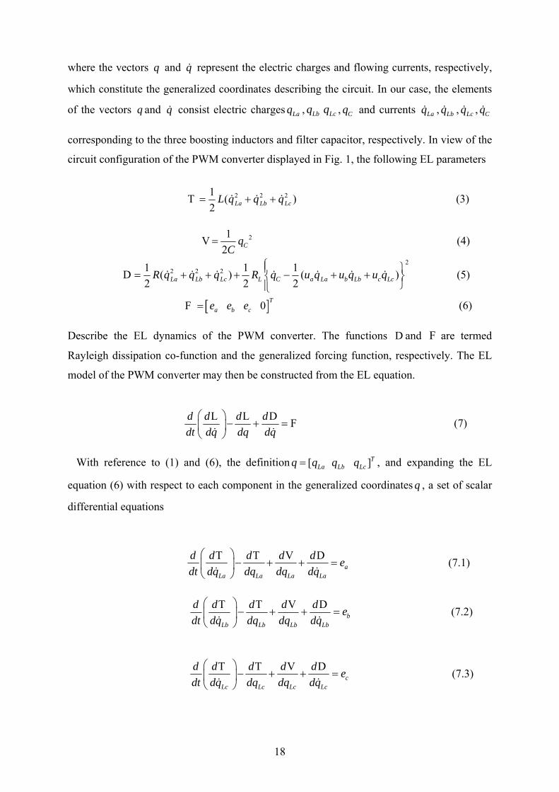
where the vectors and represent the electric charges and flowing currents, respectively,

which constitute the generalized coordinates describing the circuit. In our case, the elements

of the vectors q and consist electric charges , , and currents , , ,

corresponding to the three boosting inductors and filter capacitor, respectively. In view of the

circuit configuration of the PWM converter displayed in Fig. 1, the following EL parameters

q q&

q& Laq Lbq Lcq Cq Laq& Lbq& Lcq& Cq&

2 2 21 (2 La Lb Lc )L q q q= + +& & &T (3)

212 CqC

=V (4)

2

2 2 21 1 1( ) (2 2 2La Lb Lc L C a La b Lb c LcR q q q R q u q u q u q

⎧⎪ ⎫= + + + − + + )⎨ ⎬⎭⎪⎩

& & & & & & &D (5)

[ ]0 Ta b ce e e=F (6)

Describe the EL dynamics of the PWM converter. The functions and are termed

Rayleigh dissipation co-function and the generalized forcing function, respectively. The EL

model of the PWM converter may then be constructed from the EL equation.

D F

d d d ddt dq dq dq⎛ ⎞

− + =⎜ ⎟⎝ ⎠& &

L L D F (7)

With reference to (1) and (6), the definition , and expanding the EL

equation (6) with respect to each component in the generalized coordinates , a set of scalar

differential equations

[ TLa Lb Lcq q q q= ]

q

aLa La La La

d d d d d edt dq dq dq dq⎛ ⎞

− + + =⎜ ⎟⎝ ⎠& &

T T V D (7.1)

bLb Lb Lb Lb

d d d d d edt dq dq dq dq⎛ ⎞

− + + =⎜ ⎟⎝ ⎠& &

T T V D (7.2)

cLc Lc Lc Lc

d d d d d edt dq dq dq dq⎛ ⎞

− + + =⎜ ⎟⎝ ⎠& &

T T V D (7.3)

18

0C C C C

d d d d ddt dq dq dq dq⎛ ⎞

− + + =⎜ ⎟⎝ ⎠& &

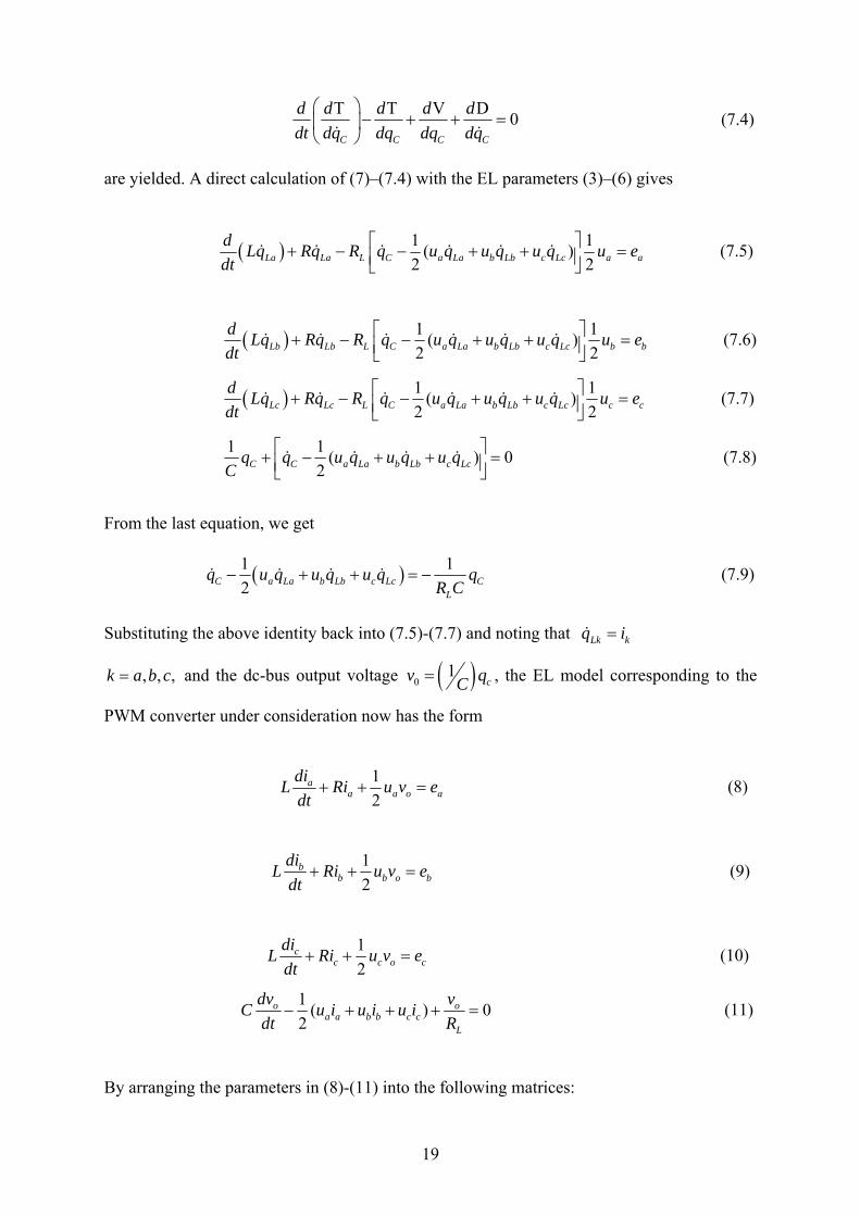
T T V D (7.4)

are yielded. A direct calculation of (7)–(7.4) with the EL parameters (3)–(6) gives

( ) 1 ( )2 2La La L C a La b Lb c Lc a a

d 1Lq Rq R q u q u q u q udt

⎡+ − − + + =⎢⎣ ⎦& & & & & & e⎤

⎥ (7.5)

( ) 1 ( )2 2Lb Lb L C a La b Lb c Lc b b

d 1Lq Rq R q u q u q u q udt

⎡ ⎤+ − − + + =⎢ ⎥⎣ ⎦& & & & & & e (7.6)

( ) 1 ( )2 2Lc Lc L C a La b Lb c Lc c c

d 1Lq Rq R q u q u q u q udt

⎡ ⎤+ − − + + =⎢ ⎥⎣ ⎦& & & & & & e (7.7)

1 1 (2C C a La b Lb c Lcq q u q u q u q

C⎡ ) 0⎤+ − + +⎢⎣ ⎦& & & & =⎥ (7.8)

From the last equation, we get

( )12C a La b Lb c Lc

L

q u q u q u qR C

− + + = −& & & &1

Cq (7.9)

Substituting the above identity back into (7.5)-(7.7) and noting that Lk kq i=&

, , ,k a b c= and the dc-bus output voltage ( )01

cv C= q , the EL model corresponding to the

PWM converter under consideration now has the form

12

aa a o

diaL Ri u v e

dt+ + = (8)

12

bb b o

dibL Ri u v e

dt+ + = (9)

12

cc c o

dicL Ri u v e

dt+ + = (10)

1 ( )2

oa a b b c c

L

dv vC u i u i u idt R

− + + + 0o = (11)

By arranging the parameters in (8)-(11) into the following matrices:

19

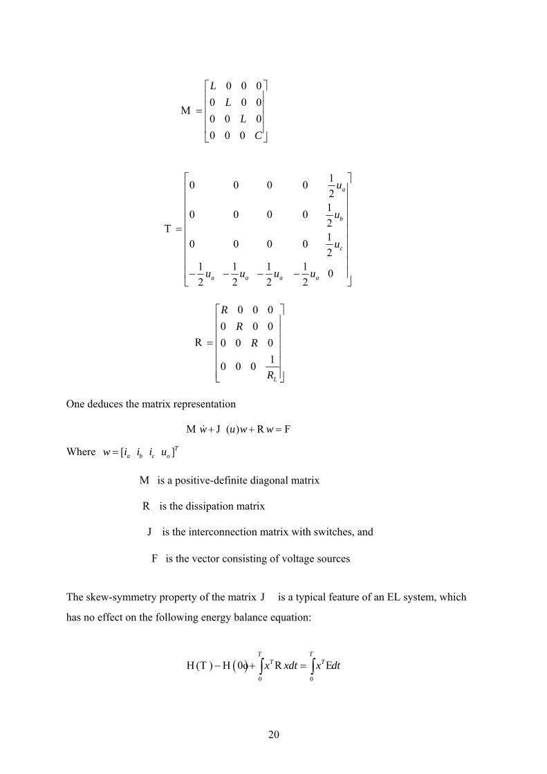
0 0 00 0 00 0 00 0 0

LL

LC

⎡ ⎤⎢ ⎥⎢ ⎥=⎢ ⎥⎢ ⎥⎣ ⎦

M

10 0 0 0210 0 0 0210 0 0 02

1 1 1 1 02 2 2 2

a

b

c

a a a a

u

u

u

u u u u

⎡ ⎤⎢ ⎥⎢ ⎥⎢ ⎥⎢ ⎥

= ⎢ ⎥⎢ ⎥⎢ ⎥⎢ ⎥− − − −⎢ ⎥⎣ ⎦

T

0 0 00 0 00 0 0

10 0 0L

RR

R

R

⎡ ⎤⎢ ⎥⎢ ⎥⎢ ⎥=⎢ ⎥⎢ ⎥⎢ ⎥⎣ ⎦

R

One deduces the matrix representation ( )w u w w+ + =&M J R F

Where [ ]Ta b c ow i i i u=

is a positive-definite diagonal matrix M R is the dissipation matrix is the interconnection matrix with switches, and J is the vector consisting of voltage sources F The skew-symmetry property of the matrix is a typical feature of an EL system, which

has no effect on the following energy balance equation:

J

( )0 0

( )T T

T Tx xdt x dt− + =∫ ∫H T H 0o R E

20

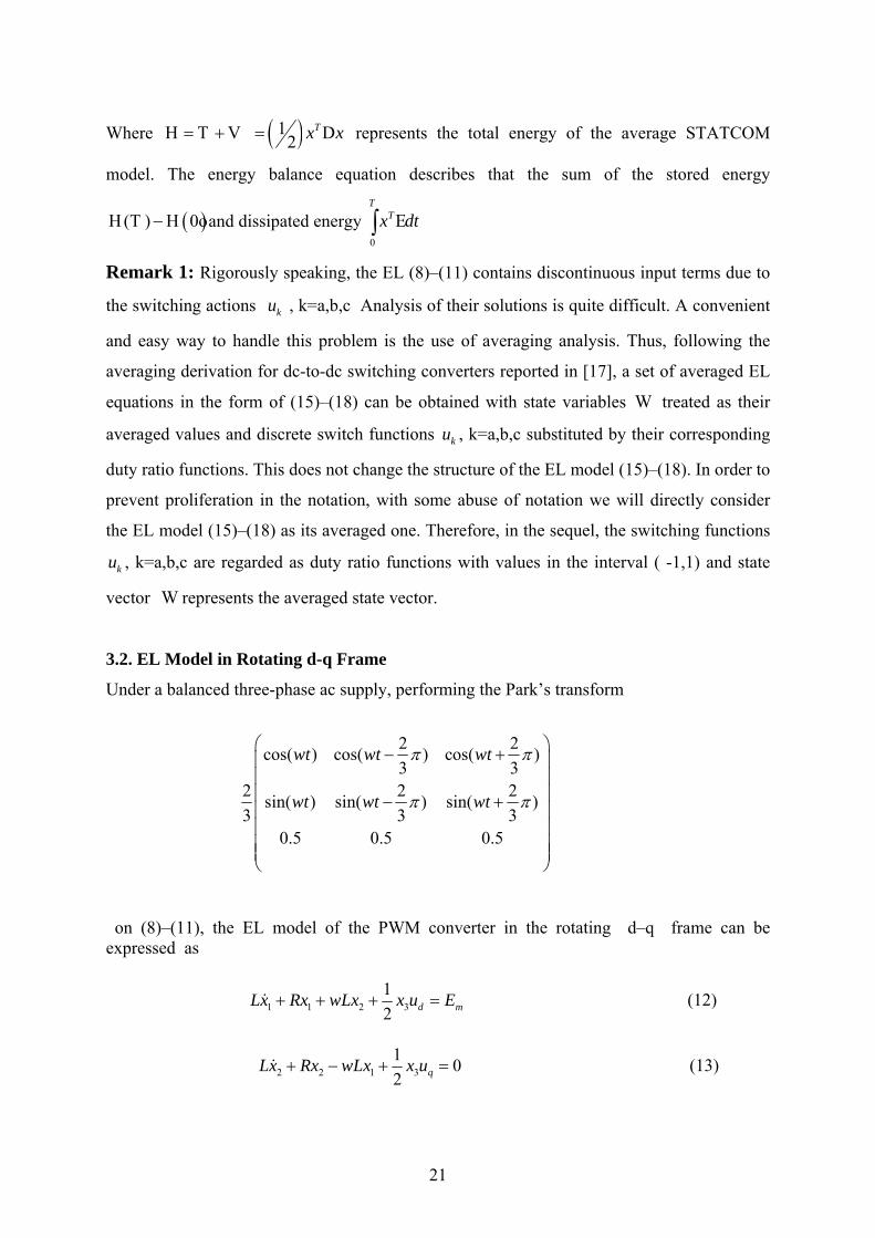
Where = +H T V ( )1

2Tx x= D represents the total energy of the average STATCOM

model. The energy balance equation describes that the sum of the stored energy

( )( )−H T H 0oand dissipated energy 0

TTx dt∫ E

Remark 1: Rigorously speaking, the EL (8)–(11) contains discontinuous input terms due to

the switching actions , k=a,b,c Analysis of their solutions is quite difficult. A convenient

and easy way to handle this problem is the use of averaging analysis. Thus, following the

averaging derivation for dc-to-dc switching converters reported in [17], a set of averaged EL

equations in the form of (15)–(18) can be obtained with state variables treated as their

averaged values and discrete switch functions , k=a,b,c substituted by their corresponding

duty ratio functions. This does not change the structure of the EL model (15)–(18). In order to

prevent proliferation in the notation, with some abuse of notation we will directly consider

the EL model (15)–(18) as its averaged one. Therefore, in the sequel, the switching functions

, k=a,b,c are regarded as duty ratio functions with values in the interval ( -1,1) and state

vector W represents the averaged state vector.

ku

W

ku

ku

3.2. EL Model in Rotating d-q Frame

Under a balanced three-phase ac supply, performing the Park’s transform

2 2cos( ) cos( ) cos( )3 3

2 2sin( ) sin( ) sin( )3 3

0.5 0.5 0.5

wt wt wt

wt wt wt 23

π π

π π

⎛ ⎞− +⎜ ⎟⎜ ⎟⎜ ⎟− +⎜ ⎟⎜ ⎟⎜ ⎟⎜ ⎟⎝ ⎠

on (8)–(11), the EL model of the PWM converter in the rotating d–q frame can be expressed as

1 1 2 312 d mLx Rx wLx x u E+ + + =& (12)

2 2 1 31 02 qLx Rx wLx x u+ − + =& (13)

21

33 1 2

2 1 1 2 03 2 2 3d q

L

xCx x u x uR

− − +& =

]T

(14)

In the transformed state equations (12)–(14), the state vector is defined as

1 2 3[ ] [Td q ox x x x i i v= = and the control input vector contains the duty ratio

functions in the synchronously rotating d-q frame. It can be demonstrated that

passivity properties of the a-b-c axis EL model are retained under the park’s transformation.

Representing the d-q model in the following matrix form.

[ Td qu u u= ]

][ Ta b cu u u u=

1 2[ ( )]x u+ + + =&M J J R x E (15)

With

0 0

0 020 03

LL

C

⎛ ⎞⎜ ⎟⎜ ⎟

= ⎜ ⎟⎜ ⎟⎜ ⎟⎝ ⎠

M = 2

10 021( ) 02

1 1 02 2

d

q

d q

u

u L

u u

⎛ ⎞⎜ ⎟⎜ ⎟⎜ ⎟= ⎜ ⎟⎜ ⎟⎜ ⎟− −⎜ ⎟⎝ ⎠

J u

1

0 00 0

0 0 0

wLwL

⎛ ⎞⎜ ⎟= −⎜ ⎟⎜ ⎟⎝ ⎠

J 0 0

0 020 0

3 L

RR

R

⎛ ⎞⎜ ⎟⎜ ⎟

= ⎜ ⎟⎜ ⎟⎜ ⎟⎜ ⎟⎝ ⎠

R x

and 00

mE⎡ ⎤⎢ ⎥= ⎢ ⎥⎢ ⎥⎣ ⎦

E

one can easily arrive at the energy balance equation.

( )0 0

( )T T

T Tx xdt x dt− + =∫ ∫H T H 0o R E (16)

22

Where = +H T V ( )12

Tx x= D represents the total energy of the average STATCOM

model. The energy balance equation describes that the sum of the stored energy

( )( )−H T H 0oand dissipated energy 0

TTx dt∫ E

23

NONLINEAR STATCOM CONTROLLER DESIGN

4. Controller Design The control strategy for STATCOM concerns with the control of ac and dc bus voltage on

both sides of STATCOM. Our goal is to achieve output voltage tracking via regulation of

input line currents. For the error state vector , the EL model of

the STATCOM model (15) can be written as

* * *[ , , Td d q q dc dce i i i i V V= − − − ]

[ ]

[ ]( )1

* *1

( )

( )

e u e e*x u x Rx

+ + +

= + + +

&

& &

2

2

D J J R

E D J J x (17)

we see that R injects damping required for asymptotic stability , and that the convergence rate

of *x to zero is improved by increasing R. One may perform a damping injection on (17) by

considering the following desired dissipation term

(18) ( )de = +R R R ss e

Where 1

2

3

0 00 00 0

s

s s

s

rr

r

⎛ ⎞⎜ ⎟= ⎜ ⎟⎜ ⎟⎝ ⎠

R s

By substituting (18) into (17), the error dynamics with the injection damping is obtained as

[ ]

[ ]( )1 2

* * *1 2

( )

( )d

s

e u e e

x u x x e

+ + +

= − + + + −

&

&

D J J R

E= D J J R R x (19)

In order to obtain desired error dynamics, (19) must require

[ ]( * * *1 2 ( ) sx u x x e+ + + − =&D J J R R x) E (20)

Which corresponds to the following scalar differential equations

* * * * *1

1 ( )2d d q dc d s d dLi Ri wLi V u r i i E+ + + − − = (21)

* * * * *2

1 ( )2q q d dc q s q qLi Ri wLi V u r i i+ − + − − = 0 (22)

*

*3

22 1 ( ) ( )3 2 3

dcdc d q s dc dc

dc

VC V u u r V VR

− + + − − =& * 0 (23)

24

In the STATCOM control, there are two broad objectives, ac and dc bus voltage that are

modified via regulation of input linear currents. Our goal is to achieve regulation of to

and to . From (21) and (22), the control variables and can be solved as

di*di

qi*qi du qu

* * *1*

2 ( )d d q s d ddc

u Ri wLi r i iV

⎡= − − + − +⎣ E⎤⎦ (24)

* * *2*

2 (q d q s qdc

u wLi Ri r i iV

⎡= − + −⎣ )q ⎤⎦ (25)

By substituting and into (23), the control law is obtained as du qu

** * * *

1*

* ** * *

2*

3 ( )2

3( )

2

ddc q d s d d

dc

q dcd q s q q

dc dc

iV wLi Ri r i iCV

i VwLi Ri r i iCV R C

E⎡ ⎤= − − + − +⎣ ⎦

⎡ ⎤+ − + − −⎣ ⎦

(26)

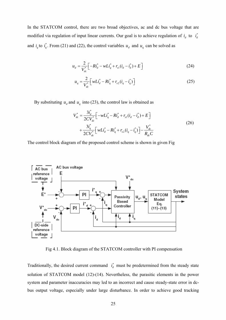
The control block diagram of the proposed control scheme is shown in given Fig

Fig 4.1. Block diagram of the STATCOM controller with PI compensation

Traditionally, the desired current command must be predetermined from the steady state

solution of STATCOM model (12)-(14). Nevertheless, the parasitic elements in the power

system and parameter inaccuracies may led to an incorrect and cause steady-state error in dc-

bus output voltage, especially under large disturbance. In order to achieve good tracking

*di

25

performance with strong robustness, the classical PI controller is used to regulate the d-q axis

current command and . Henceforth, the passivity-based control technique mentioned

above is readily employed to the design of a STATCOM controller.

*di

*qi

26

SIMULATION RESULTS AND DISCUSSION

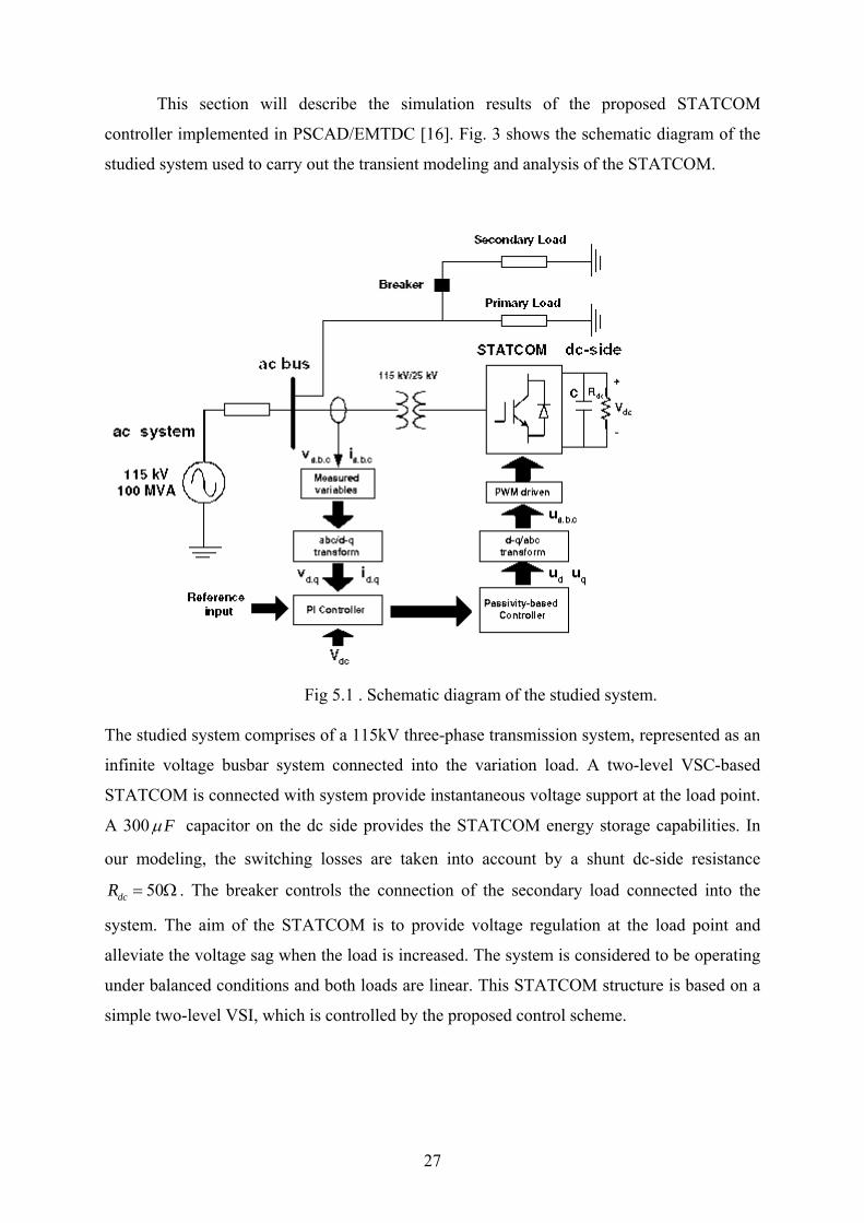
This section will describe the simulation results of the proposed STATCOM

controller implemented in PSCAD/EMTDC [16]. Fig. 3 shows the schematic diagram of the

studied system used to carry out the transient modeling and analysis of the STATCOM.

Fig 5.1 . Schematic diagram of the studied system. The studied system comprises of a 115kV three-phase transmission system, represented as an

infinite voltage busbar system connected into the variation load. A two-level VSC-based

STATCOM is connected with system provide instantaneous voltage support at the load point.

A 300 Fµ capacitor on the dc side provides the STATCOM energy storage capabilities. In

our modeling, the switching losses are taken into account by a shunt dc-side resistance

. The breaker controls the connection of the secondary load connected into the

system. The aim of the STATCOM is to provide voltage regulation at the load point and

alleviate the voltage sag when the load is increased. The system is considered to be operating

under balanced conditions and both loads are linear. This STATCOM structure is based on a

simple two-level VSI, which is controlled by the proposed control scheme.

50dcR = Ω

27

The parameters of the studied system are listed in table 5.1

TABLE 5.1

SYSYEM PARAMETERS

Ac source voltage E 115kV

Line resistance R 0.5Ω

Line inductor L 20mH

dc- side capacitor C 300 Fµ

dc-side resistance dcR 50 Ω

Line frequency w 314 rad/s

A block diagram of the proposed control scheme for designing STATCOM controller is

shown in Fig. 3. First, the ac bus voltage, current and the dc-side voltage are measured to

construct the STATCOM model based on d-q frame. The control strategy for STATCOM

concerns with the control of ac and dc bus voltage on both sides of STATCOM. The dual

control objectives are met by generating appropriate current reference and then by regulating

those currents in the classical PI controller. The parameters of the PI controller are

determined by a repeated study of the system responses under various operating conditions.

The PI controller settings, which give the best responses under the various conditions are

listed below.

• dc bus regulator: 0.01, 0.3pd idK K= =

• ac bus regulator 2, 10pq iqK K= =

Now, the switching function and can be determined via the passivity-based controller

to counteract various disturbance from (24) and (25). Finally, the sinusoidal pulse width

modulation (SPWM) strategy is employed to generate the switching pattern from the

switching function and .

du qu

, ,a bu u cu

28

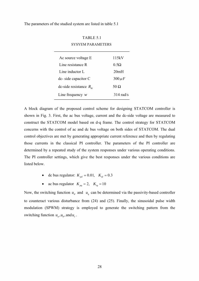
A diagram of the studied system with a STATCOM in the PSCAD environment is presented

in Fig.4.

Fig.5.2 Studied system with STATCOM in PSCAD/EMTDC 5.3 SIMULATION RESULTS Simulation results were carried out to demonstrate that the nonlinear STATCOM controller

can provide both voltage regulation and reactive power compensation at the load point when

the load is increased. In the simulation interval 0.8-1.2 s, the secondary load is increased by

closing the breaker.

29

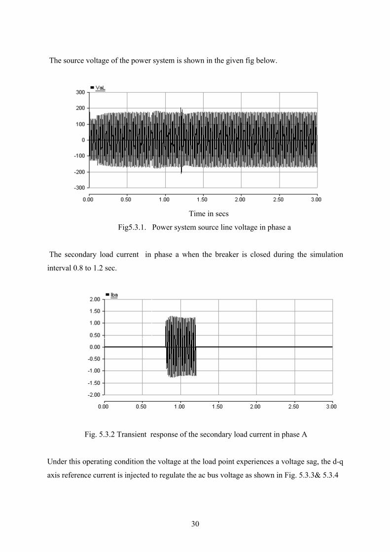
The source voltage of the power system is shown in the given fig below.

Time in secs

Fig5.3.1. Power system source line voltage in phase a

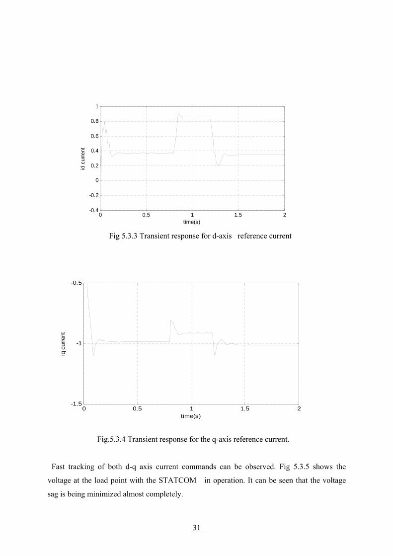
The secondary load current in phase a when the breaker is closed during the simulation

interval 0.8 to 1.2 sec.

Fig. 5.3.2 Transient response of the secondary load current in phase A

Under this operating condition the voltage at the load point experiences a voltage sag, the d-q

axis reference current is injected to regulate the ac bus voltage as shown in Fig. 5.3.3& 5.3.4

30

0 0.5 1 1.5 2

-0.4

-0.2

0

0.2

0.4

0.6

0.8

1

time(s)

id c

urre

nt

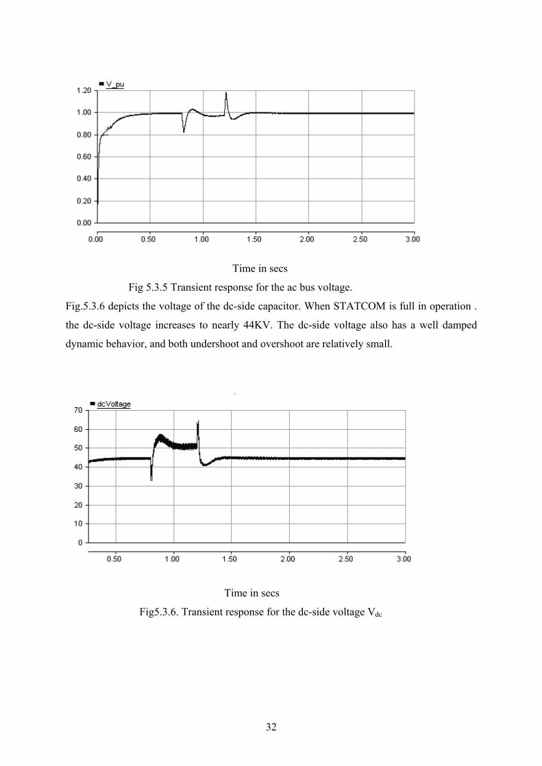
Fig 5.3.3 Transient response for d-axis reference current

0 0.5 1 1.5 2-1.5

-1

-0.5

time(s)

iq c

urre

nt

Fig.5.3.4 Transient response for the q-axis reference current. Fast tracking of both d-q axis current commands can be observed. Fig 5.3.5 shows the

voltage at the load point with the STATCOM in operation. It can be seen that the voltage

sag is being minimized almost completely.

31

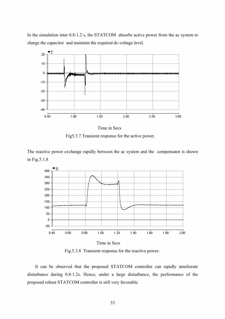
Time in secs

Fig 5.3.5 Transient response for the ac bus voltage.

Fig.5.3.6 depicts the voltage of the dc-side capacitor. When STATCOM is full in operation .

the dc-side voltage increases to nearly 44KV. The dc-side voltage also has a well damped

dynamic behavior, and both undershoot and overshoot are relatively small.

Time in secs

Fig5.3.6. Transient response for the dc-side voltage Vdc

32

In the simulation inter 0.8-1.2 s, the STATCOM absorbs active power from the ac system to

charge the capacitor and maintain the required dc-voltage level.

Time in Secs

Fig5.3.7 Transient response for the active power.

The reactive power exchange rapidly between the ac system and the compensator is shown

in Fig.5.1.8

Time in Secs

Fig.5.3.8 Transient response for the reactive power.

It can be observed that the proposed STATCOM controller can rapidly ameliorate

disturbance during 0.8-1.2s. Hence, under a large disturbance, the performance of the

proposed robust STATCOM controller is still very favorable.

33

5.2 DISCUSSIONS

First, the ac bus voltage, current and the dc-side voltage are measured to construct the

STATCOM model based on d-q frame. The control strategy for STATCOM concerns with

the control of ac and dc bus voltage on both sides of STATCOM. The dual control objectives

are met by generating appropriate current reference and then by regulating those currents in

the classical PI controller.

When the secondary load is increased in the interval 0.8 to 1.2 by closing the breaker,

the STATCOM is provide voltage regulation at the load point and alleviate the voltage sag

when the load is increased. The system is considered to be operating under balanced

conditions and both loads are linear. The reactive power exchange between the ac system and

the compensator is discussed. Hence, under a large disturbance, the performance of the

proposal robust STATCOM controller is still very favorable.

34

CONCLUSION AND SCOPE FOR FUTURE WORK

6.1 CONCLUSION

The ability of the STATCOM device in compensating the power system and stabilize

the bus voltage with no transient disturbances on the power system during the transition of

increasing or decreasing the reactive power compensation. We have proposed a design

procedure of passivity-based nonlinear STATCOM controller for providing both reactive

power compensation and voltage regulation at the point of connection. The mathematical

model of STATCOM was shown to be EL systems corresponding to a set of EL parameters.

The passivity-based control technique allows relatively fast control of the d-q current with

good dynamic performance of the overall system. The proposed STATCOM controller, that

was investigated by PSCAD/EMTDC has been validated. Simulation result shows that the

proposed controller can effectively enhance transient stability of the power system even in

the presence of variation load.

6.2 SCOPE FOR FUTURE WORK

Improvement can be brought in the design of the passivity-based nonlinear STATCOM

controller. This can also be done either in MATLAB or C. In order to achieve good tracking

performance we may also use fuzzy controller to regulate the d-q axis current commands. We

also setup the experimental results for the comparison study of the 6-pulse STATCOM.

35

REFERENCES

[1] C. S. de Araujo and J. C. Castro, “Vectors analysis and control of advanced static VAR

compensators,” IEE Proceedings-C, vol. 140, no. 4, Jul. 1993, pp. 299–306.

[2] A. H. Norouzi and A. M. Sharaf, “Two control scheme to enhance the dynamic

performance of the STATCOM and SSSC,” IEEE Trans. On Power Delivery, vol. 20,

no. 1, Jan. 2005, pp. 435–442.

[3] R. Mienski, R. Pawelek, and I. Wasiak, “Shunt compensation for power quality

improvement using a STATCOM controller: modeling and simulation,” IEE Proc.-

Gener. Transm. Distrib., vol. 151, no. 2, , Mar. 2004,pp. 274– 280.

[4]Hung-Chi Tsai, Chia-Chi Chu. Member, IEEE, and Sheng-Hui Lee Student Member,

IEEE “ Passivity-based Nonlinear STATCOM Controller Design for Improving Transient

Stability of Power Systems” 2005 IEEE/PES Transmission and Distribution Conference

& Exhibition: Asia and Pacific Dalian, China

[5] N. C. Schaoo, B. K. Panigrahi, P. K. Dash, and G. Panda, “Application of a multivariable

feedback linearization scheme for STATCOM control,”Electric Power System Research,

vol. 62, no. 2, Jul. 2002, pp. 81–91.

[6] H. Sira-Ramirez, R. A. Perez-Moreno, R. Ortega, and M. Garcia-Esteban, “Passivity-

based controllers for the stabilization of DC-to-DC power converters,” Automatica, vol.

33, no. 4, pp. 499–513.

[7] G. E. Valderrama and P. M. amd A. M. Stankovic, “Reactive power and unbalance

compensation using STATCOM with dissipativity-based control,” IEEE Trans. on

Control Systems Technology, vol. 9, no. 5, Sep. 2001,pp.718–727.

[8] H. Sira-Ramierz, R. A. Perez-Moreno, R. Ortega, and M. Garcia-Esteban, “Passivity-

based controllers for the stabilization of DC-to-DC,” Automatica, vol. 33, no. 4, 97

pp. 499– 512,

[9] T. S. Lee, “Lagrangian modeling and passivity-based control of three phase AC/DC

voltage-source converters,” IEEE Trans. on Industrial Electronics, vol. 51, no. 4, , Aug.

2004 pp.892– 902

[10] T.-S. Lee, “Input-output linearization and zero-dynamics control of three-phase AC/DC

voltage-source converters,” IEEE Trans. Power Electron., vol. 18, pp. 11–22, Jan. 2003.

[11] V. Blasko and V. Kaura, “A new mathematical model and control of a three-phase AC-

DC voltage source converter,” IEEE Trans. Power Electron., vol. 12, pp. 116–123, Jan.97

[12] S. Mori, K. Matsuno, M. Takeda, M. Seto, Development of a large static var generator

36

Using self-commutated inverters for improving power systems stability, IEEE

[13] C. A. Desoer and C.-A. Lin, “Tracking and disturbance rejection of MIMO nonlinear

systems with PI controller,” IEEE Trans. Automat. Contr., vol. AC-30, pp. 861–866,

Sept. [27] B. K. Bose, Modern Power Electronics and AC Drives. Upper Saddle River,

NJ: Prentice –Hall, 2001.1985.

[14] M. T. Tsai andW. I. Tsai, “Analysis and design of three-phase AC-to-DC converters

with high power factor and near-optimum feedforward,” IEEE Trans. Ind. Electron., vol.

46, pp. 263–273, June 1999.

[15] PSCAD/EMTDC Version 3.0. Manitoba HVDC Research Centre Inc.,2001.

[16] R. Wu, S. B. Dewan, and G. R. Slemon, “A PWM ac-to-dc converter with fixed

switching frequency,” IEEE Trans. Ind. Applicat., vol. 26, pp. 880–885, Sept./Oct. 1990.

[17] J. W. Dixon and B. T. Ooi, “Indirect current control of a unity power factor sinusoidal

current boost type three phase rectifier,” IEEE Trans. Ind. Electron., vol. 35, pp. 508–515,

Aug. 1988.

[18] A. Draou, Y. Sato, and T. Kataoka, “A new state feedback based transient control of

PWM AC to DC type converters,” IEEE Trans. Power Electron., vol. 10, pp. 716–724,

Nov. 1995.

[19] S. Hiti, D. Borojecvic, R. Ambatipudi, R. Zhang, and Y. Jiang, “Average current control

of three-phase PWM boost rectifier,” in Conf. Rec. IEEE PESC’95, June 1995, pp. 131–

137.

[20] D.-C. Lee, G.-M. Lee, and K.-D. Lee, “DC-bus voltage control of three-phase AC/DC

PWM converters using feedback linearization,” IEEE Trans. Ind. Applicat., vol. 36, pp.

826–833, May/June 2000.

[21] P. Krein, J. bentsman, R. Bass, and B. Lesieutre, “On the use of averaging for the

Analysis of power electronic systems,” IEEE Trans. Power Electron., vol. 5, pp. 182–

190, Apr. 1990.

[22] C. A. Desoer and C.-A. Lin, “Tracking and disturbance rejection of MIMO nonlinear

systems with PI controller,” IEEE Trans. Automat. Contr., vol. AC-30, pp. 861–866,

Sept. 97

[23] Z. Xu, L.R. Hunt, “On the largest input-output linearizable subsystem”, IEEE

Transactions on Automatic control 41 (1) (1996) 128-132.

37