Improving the braking performance of a vehicle with ABS and a semi-active suspension system on a rough road Herman A. Hamersma1 & P. Schalk Els2

Department of Mechanical and Aeronautical Engineering University of Pretoria, South Africa 1hhamersma@gmail.com, 2schalk.els@up.ac.za

Abstract

Rapid advances have been made in the field of vehicle dynamics in terms of improving the ride, handling and safety using actuators and control systems. Optimising a vehicle’s ride comfort or handling has led to the development of semi-active suspension systems. Anti-lock braking systems (ABS) have resulted in significant improvements in vehicle braking whilst maintaining directional control over the vehicle. These advances have improved vehicle and occupant safety in general, but there are often some trade-offs. For example, the stopping distance of a vehicle fitted with ABS on an undulating road is significantly increased compared to braking without ABS. This has severe implications, especially in the off-road vehicle industry. The effects of spring and damper characteristics on the braking performance of a sports-utility-vehicle (SUV) on hard rough terrain are investigated. The approach is simulation based, using an experimentally validated full vehicle model of the SUV, built in Adams in co-simulation with MATLAB and Simulink. The simulations were performed on measured road profiles of a Belgian paving and parallel corrugations (or a washboard road). The results indicate that the suspension system has a significant impact on the braking performance, resulting in differences in stopping distances of up to 9m. Keywords: off-road vehicles, ABS systems, semi-active suspension, tyre modelling, multi-body dynamics modelling

Nomenclature

Table 1 - Nomenclature of symbols

Symbol Description Unit 𝒇 Coefficient of friction [Dimensionless] 𝒑𝒂 Brake line hydraulic pressure [Pa] 𝒓𝒊 Inner brake pad radius [m] 𝒓𝒐 Outer brake pad radius [m] 𝑹𝒆𝒇𝒇 Effective rolling radius [m] 𝑻 Brake torque [Nm] 𝑽 Vehicle speed [m/s] ∆𝜽 Brake pad angle [rad] 𝝎 Wheel angular speed [rad/s]

1

1 Introduction

Stopping in the shortest possible distance without losing control over a vehicle is probably the most important active safety requirement of any vehicle that can prevent accidents or at least lessen the impact. Significant advances have been made since the dawn of brakes on vehicles, most notably the development of anti-lock brake systems (ABS). Prior to discussing how ABS works, it is important to understand the friction generation mechanism of tyres. A tyre’s friction generation mechanism is due to adhesion and hysteresis between the tyre and the road in the contact patch. Adhesion arises due to the intermolecular bonds between the tyre and the road surface while hysteresis is due to the deformation of the tyre over a rough road surface [1]. The result of these phenomena is that the friction coefficient between the tyre and the road surface relies on slip between the tyre and the road. The longitudinal friction coefficient is typically characterised as a function of longitudinal wheel slip. Longitudinal wheel slip on a flat road is given by Equation (1) [1]. Examples of typical longitudinal friction coefficients for different vertical loads are shown in Figure 1. The data used in Figure 1 is from the Pacejka-model used in this study (further discussion in Section 2.4).

Figure 1 – Longitudinal friction coefficient as a function of longitudinal slip for various vertical loads

%𝑠𝑙𝑖𝑝 =𝑉 − 𝜔𝑅𝑒𝑓𝑓

𝑉× 100% (1)

Curves similar to those shown in Figure 1 may be obtained for the lateral friction coefficient, usually as a function of side-slip angle. From Figure 1 one may conclude that braking with longitudinal slip at approximately 15% results in maximum brake force and thereby the highest deceleration and the shortest possible braking distance will be attained. However, when the tyre is generating maximum

2

longitudinal force (for example during braking) the tyre cannot generate any lateral force [1]. Since lateral force is essential to controlling the lateral stability of the vehicle, braking at maximum longitudinal force may result in an uncontrollable or unstable vehicle. This led to the development of ABS. When the vehicle brakes are initially applied, the tyre deflects, generating longitudinal slip that results in a corresponding longitudinal force as dictated by the relationship indicated in Figure 2. If the longitudinal force exceeds the available friction force, the wheel locks up almost instantaneously.

Figure 2 – ABS cycling process

ABS senses when wheel lock-up occurs or is about to occur and reduces the hydraulic brake pressure accordingly. This not only prevents the wheel from locking but also generates some capacity for the development of lateral force between the tyres and the road that helps to maintain directional control [2]. Once the control system detects that the wheel is not locked and spinning freely, the brake pressure is gradually reapplied. This process is then repeated until the brake is released by the driver or the vehicle speed reduces below a set value [2]. This is the cycling indicated in Figure 2. The ABS cycle has three distinct phases, namely hold, reduce or increase pressure. Initially, as the driver applies pressure to the brake pedal, the hydraulic pressure rises and the wheel is braked. The wheel speed thus decreases, but ABS has no control effect at this stage. If the wheel speed decreases too rapidly, the control system detects that lockup is imminent. At this stage the inlet valve from the master cylinder is closed and the hydraulic pressure cannot be increased further (the

3

hold phase). If the wheel speed continues to decrease the outlet valve is opened and the hydraulic pressure is reduced as fluid drains back to the reservoir. With a reduction in brake pressure the wheel speed starts to increase again. If the wheel speed increases so that it is no longer braking acceptably, the controller again gradually increases the brake pressure, even if the driver presses harder on the brake pedal [2]. This process is repeated several times per second on each wheel. It may be noted that the only feedback necessary for the implementation of ABS is the wheel speed (further discussion in Section 2.2). The wheel speed is used to calculate the wheel deceleration and in more modern algorithms to estimate the longitudinal wheel slip. Therein lays the assumption that the effective rolling radius stays relatively constant – this implies that the road surface is relatively smooth and the longitudinal slip is determined with Equation (1). When driving over rough terrain, such as a Belgian paving or a dirt road with corrugations (a washboard road), ABS systems may not be beneficial. Not only is the effective rolling radius changing due to undulations in the road surface, the vertical and torsional dynamics of the wheel may be excited to such an extent that contact between the tyre and the road is lost or that the tyre starts oscillating. The tyre oscillation has a significant effect on the performance of an ABS system, as discussed by Adcox et al. [3]. The situation is further complicated by the so-called run-in effect of tyre force generation. Gillespie [1] describes the run-in effect stating that a tyre’s response to a step input is not instantaneous. The lag is related to the rotation of the tyre, typically taking between one-half and one full revolution of the wheel to reach the steady-state force condition. A varying vertical load on the tyre, as is the case when driving over a rough road, thus further complicates the optimum application of ABS. When the wheel load increases, the size of the contact patch is increased with rubber that is not deformed. The ‘new’ rubber has to deform before it generates a significant horizontal force, which lags the increase in vertical load. In contrast, when the wheel load decreases, the contact patch area decreases and the force generated is decreased instantaneously. Furthermore, due to the low damping present in the tyre, natural frequencies (specifically the torsional modes) may be excited due to the terrain input and the periodic braking input from the ABS. The net effect of this process is a reduction in the brake force and increased stopping distances [2]. Initial brake tests were done on a flat road and an undulating road and it was found that the suspension settings have a small effect on the braking performance on a flat road, but that there are some advantages to be gained by adjusting the suspension on a flat road. However, initial results showed that a significant improvement can be made in the braking performance on a rough road and the study will focus on the improvement possible on rough roads [4]. The research question of this paper may thus be defined as: Can the stopping distance on a rough road of a vehicle equipped with ABS and a semi-active suspension be improved by changing the suspension characteristics? Similar studies have been performed, but these studies were mainly limited to modifying the damper characteristics or with the use of simplified models such as a quarter car model and a pitch-bounce model [5]. The current study focuses on severely undulating roads with a Displacement Spectral Density (DSD) similar to that of an ISO 8608 Class D road on a test vehicle fitted with both adjustable spring and adjustable damper settings by using an experimentally validated full vehicle model. The test vehicle used for this study is a Land Rover Defender (see Section 2.1), not a passenger car and hence wheel travel and body rotation (roll and pitch specifically due to a high

4

centre of gravity, a generally soft suspension and high profile tyres) potentially plays a more significant role.

2 Mathematical models

The mathematical model employed in this study consists of the full vehicle model (including semi-active suspension), the ABS control algorithm as well as road and tyre models.

2.1 Full vehicle model

The vehicle used as experimental platform for this study is a 1997 Land Rover Defender. The Land Rover has been fitted with a hydro-pneumatic semi-active suspension called the four-state semi-active suspension system (4S4) [6]. The 4S4 features two damper packs, fitted with bypass valves, and two gas accumulators per strut with a solenoid valve to isolate the bigger accumulator as shown in Figure 3. The two gas accumulators (one with a volume of 0.1l and the other 0.4l) are used as air springs with floating pistons to separate the gas and the hydraulic fluid used for damping. Switching the solenoid valve so that both gas accumulators are used results in a very soft spring, while switching so that only the small accumulator is used results in a hard spring. The bypass valves are used to bypass the damper packs and obtain a high damping and low damping settings. Both bypass valves, as shown in Figure 3, are opened for the low damping setting and both are closed for the high damping setting, irrespective of the spring setting chosen. The net result is a semi-active suspension system with two damper and two spring characteristics. The spring and damper characteristics can be changed to either a ‘ride comfort’ mode, using the soft spring and low damping, or a handling mode using the hard spring and high damping. The spring and damper characteristics are given in Figures 4 and 5 [7].

Figure 3 – Schematic of 4S4 suspension unit

5

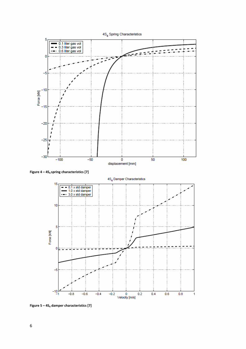
Figure 4 – 4S4 spring characteristics [7]

Figure 5 – 4S4 damper characteristics [7]

6

A model of the 4S4 suspension unit was developed by Thoresson et al. [7] and included in an Adams [8] and MATLAB/Simulink [9] co-simulation model of the full vehicle. The unconstrained degrees of freedom of the full model are given in Table 2 and a graphical representation of the front and rear suspension (as modelled in Adams) is shown in Figure 6 [7]. The experimental validation may be seen in Thoresson et al. [7]. Table 2 – Unconstrained degrees of freedom of full vehicle model

Body Unconstrained Degrees of Freedom

Associated Motions

Vehicle body (two rigid bodies)

7 Body torsion Longitudinal, Lateral, Vertical translation and Roll, Pitch and Yaw Rotation

Front axle 2 Roll and vertical translation Rear axle 2 Roll and vertical translation Wheels 4 Rotation

Figure 6 – Model of the rear (left image) and front (right image) suspension as modelled in Adams [7]

2.2 ABS algorithm

The ABS algorithm used in the simulation model was developed by Savitski et al. [10]. The algorithm is presented schematically in Figure 7. It may be noted in Figure 7 that the ABS algorithm uses the longitudinal wheel slip (calculated with Equation (1)) and the wheel’s angular acceleration to determine when lock-up is about to occur. The algorithm uses fixed thresholds and no modification is done to the algorithm dependent on the surface. This is done to minimize the number of variables that influence the braking performance of the vehicle and may be addressed in future studies. The

7

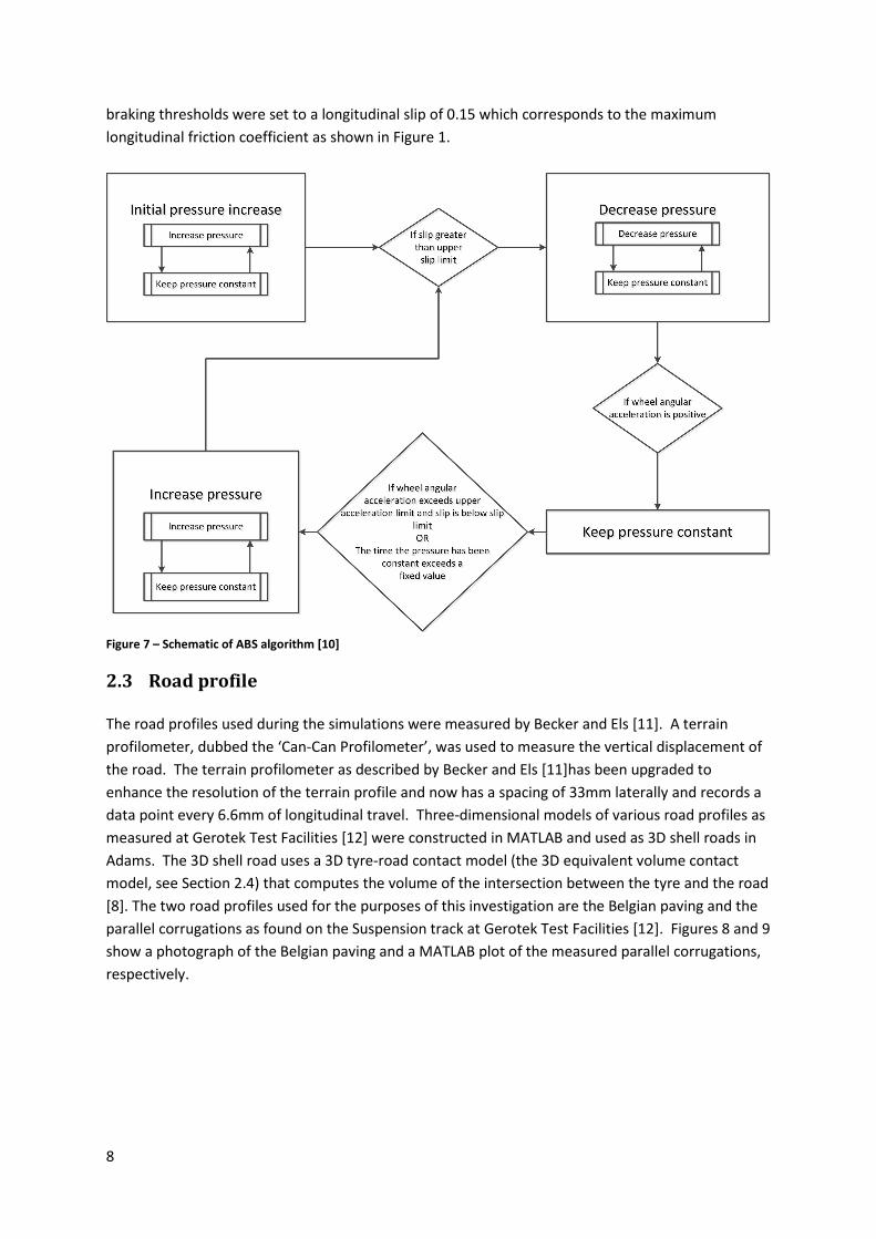
braking thresholds were set to a longitudinal slip of 0.15 which corresponds to the maximum longitudinal friction coefficient as shown in Figure 1.

Figure 7 – Schematic of ABS algorithm [10]

2.3 Road profile

The road profiles used during the simulations were measured by Becker and Els [11]. A terrain profilometer, dubbed the ‘Can-Can Profilometer’, was used to measure the vertical displacement of the road. The terrain profilometer as described by Becker and Els [11]has been upgraded to enhance the resolution of the terrain profile and now has a spacing of 33mm laterally and records a data point every 6.6mm of longitudinal travel. Three-dimensional models of various road profiles as measured at Gerotek Test Facilities [12] were constructed in MATLAB and used as 3D shell roads in Adams. The 3D shell road uses a 3D tyre-road contact model (the 3D equivalent volume contact model, see Section 2.4) that computes the volume of the intersection between the tyre and the road [8]. The two road profiles used for the purposes of this investigation are the Belgian paving and the parallel corrugations as found on the Suspension track at Gerotek Test Facilities [12]. Figures 8 and 9 show a photograph of the Belgian paving and a MATLAB plot of the measured parallel corrugations, respectively.

8

Figure 8 – Can-can profilometer measuring the Belgian paving [10] (see online version for colour image)

Figure 9 – Parallel corrugations (see online version for colour image) Although both the Belgian paving and the parallel corrugations are rough (Becker and Els [11] found that the Displacement Spectral Density (DSD) of the Belgian paving is similar to an ISO 8608 [13] Class D road), the main difference lies in the type of vertical excitation the wheels and suspension system receives. The Belgian paving is designed so that a broad spectrum of frequencies is excited, as close to random excitation as possible, although this is not quite the case (Becker and Els [11] found two distinct peaks in the DSD, corresponding to the length of the cobblestones and the gap between the cobblestones). The parallel corrugations, in contrast to the Belgian paving, are not

9

aimed at random excitation of the wheels and suspension system. The excitation is periodic and simulates driving on worn-out dirt roads. The excitation frequency on the parallel corrugations is directly proportional to the vehicle speed.

2.4 Brake and tyre model

The brakes were included in the Adams model as torques acting on the wheels. The torque is determined as a function of the hydraulic brake pressure (see Equation (2) [14]) with a MATLAB function and is then given as input to the Adams model via Simulink.

𝑇 =12

(∆𝜃)𝑓𝑝𝑎𝑟𝑖�𝑟𝑜2 − 𝑟𝑖2� (2)

For experimental validation the vehicle was instrumented with a proximity switch to measure the wheel angular velocity on the wheel hub (60 pulses per revolution) and a pressure transducer in the brake line to measure the hydraulic pressure applied. A frequency to voltage converter was used to convert the proximity switch pulses to a voltage representing wheel speed. Brake tests were performed from approximately 80km/h to a full stop – the brakes thus had to dissipate the kinetic energy of the full vehicle. Simulations were then performed using a full vehicle simulation model using the measured brake line hydraulic pressure as input to the model and the simulated and measured wheel speed was compared for validation purposes. Figure 10 compares the experimentally measured wheel speed with the modelled wheel speed and it may be seen that the modelled and the measured wheel speed corresponds closely although some important measurement noise is present on the measured wheel speed. The model of the brakes used in the simulation environment was thus deemed experimentally validated. The tyre model used for this investigation is a Magic Formula tyre model as developed by Bakker et al. [15] in conjunction with the 3D equivalent volume contact method as implemented in Adams [8] and the friction coefficient is given in Figure 1. The 3D equivalent volume contact method computes the volume of intersection between the tyre and the road. From this intersection the method computes an equivalent plane’s effective normal penetration, effective tyre to road contact point and the effective road friction. The contact algorithm is based on a representation of the road using tessellated triangles and the cross-section of the carcass. A series of 2D circle contacts to the 3D road is then used (each 2D circle represents an equal section of the tyre shape) [8]. There are significant improvements that can be made to this model of the tyre, using technology such as FTire [16] and more recent formulations of the Magic Formula model [17]. Parameterisation data for these tyre models are not yet available for the tyres fitted to the test vehicle and the development and experimental validation of improved models fall outside the scope of this investigation. A previous investigation found that the 3D equivalent volume contact method yields the best results when negotiating terrain similar to the roads to be investigated in this study [18] [4].

10

Figure 10 – Validation of the brake model used for simulation

3 Simulation results

The possible improvements that could be achieved by modifying the vehicle’s suspension characteristics were investigated by using four gas volumes and four damping scale factors. A lower gas volume results in higher spring stiffness and a higher damping scale factor indicates higher damping being present. The gas volume and damping scale factors were varied for the front and rear suspension separately, resulting in 256 combinations per road profile. The gas volumes and damping scale factors chosen for this investigation lie within the extremities of the physical suspension system. The gas volume can be changed during the gas charging process without altering the current hardware. The damper settings can be changed by replacing the current on-off valve with a proportional valve, hence achieving continuously variable damping settings. Although some of the suspension configurations investigated are at this stage physically unattainable on the test vehicle, the goal of the investigation is to identify improvements possible to the braking performance on a rough road by varying the suspension settings when the ABS is activated during an emergency stop. Fortunately the model provides for these configurations. Initial studies were done with only the physically attainable properties but the identification of a pattern showing the improvement on the braking performance of the vehicle was difficult and hence more damper and spring settings were investigated. The influences of four variables are thus being investigated, namely:

1. Gas volume (or spring constant) 2. Damping scale factor (or damping coefficient)

11

3. Different front and rear suspension characteristics 4. Different road profiles

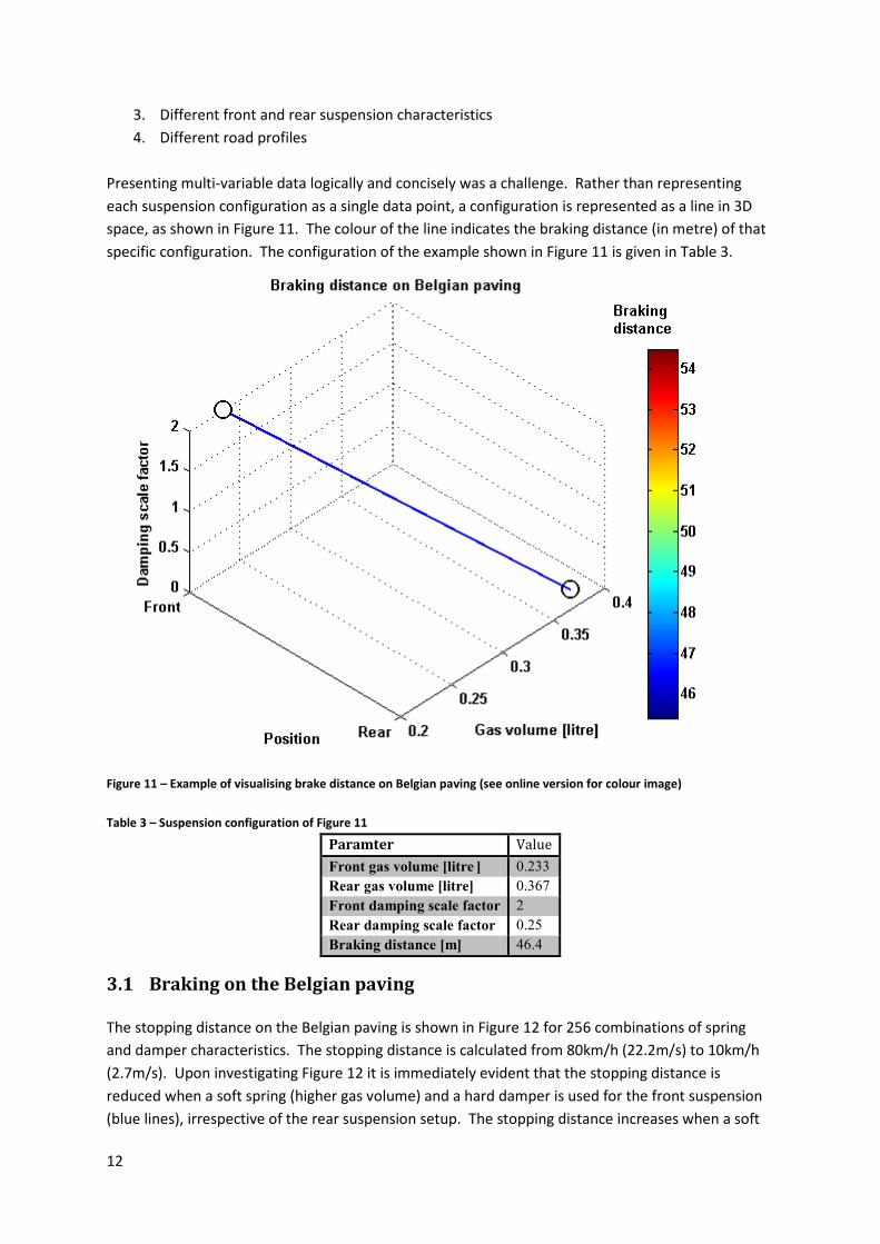
Presenting multi-variable data logically and concisely was a challenge. Rather than representing each suspension configuration as a single data point, a configuration is represented as a line in 3D space, as shown in Figure 11. The colour of the line indicates the braking distance (in metre) of that specific configuration. The configuration of the example shown in Figure 11 is given in Table 3.

Figure 11 – Example of visualising brake distance on Belgian paving (see online version for colour image) Table 3 – Suspension configuration of Figure 11

Paramter Value Front gas volume [litre ] 0.233 Rear gas volume [litre] 0.367 Front damping scale factor 2 Rear damping scale factor 0.25 Braking distance [m] 46.4

3.1 Braking on the Belgian paving

The stopping distance on the Belgian paving is shown in Figure 12 for 256 combinations of spring and damper characteristics. The stopping distance is calculated from 80km/h (22.2m/s) to 10km/h (2.7m/s). Upon investigating Figure 12 it is immediately evident that the stopping distance is reduced when a soft spring (higher gas volume) and a hard damper is used for the front suspension (blue lines), irrespective of the rear suspension setup. The stopping distance increases when a soft

12

damper is used for the front suspension. These best and worst case scenarios are isolated in Figures 13 and 14. The shortest stopping distance on the Belgian paving was 45.4m and the longest stopping distance was 54.4m, a difference of 9.0m.

Figure 12 - Braking distance for various suspension configurations on Belgian paving (see online version for colour image)

From Figure 13 it can be seen that the five best suspension configurations are with the same damping scale factor (1.417) for the front suspension. The braking performance is improved with a low damping scale factor for the rear suspension (0.25). The shortest stopping distance was achieved with a gas volume of 0.367l on the front suspension and a gas volume of 0.5l at the rear suspension. Figure 13 seems to indicate that the stiffness of the suspension has a smaller impact on the stopping distance. Higher damping in the front and lower damping in the rear leads to the shortest stopping distance on the Belgian paving. Figure 14 shows that low damping at the front and high damping at the rear increases the stopping distance. While the spring stiffness of the rear suspension does not significantly influence the stopping distance, the combination of low spring stiffness and low damping on the front suspension dramatically increases the stopping distance.

13

Figure 13 – Five best suspension configurations on the Belgian paving (see online version for colour image)

Figure 14 – Five worst suspension configurations on the Belgian paving (see online version for colour image)

14

3.2 Braking on the parallel corrugations

Figure 15 shows the stopping distance on the parallel corrugations. The shortest stopping distance was 41.8m and the longest stopping distance 43.7m, a difference of 1.9m. In Figure 15 it may be seen that the shortest stopping distances are given for suspension configurations with higher damping in the rear. The stopping distance increases as the damping is reduced on the front suspension. Figures 16 and 17 show the best and worst braking performance on the parallel corrugations, respectively.

Figure 15 – Braking distance on the parallel corrugations (see online version for colour image) In Figure 16 it can be seen that the best braking configurations were predominantly achieved with a hard spring on the front suspension and high damping on the rear suspension. The worst braking performance on the parallel corrugations were for suspension configurations with low damping in the front and rear, with the spring stiffness having little impact on the braking performance. Table 4 shows the best and worst suspension configurations for both the Belgian paving and the parallel corrugations.

15

Figure 16 – Five best suspension configurations for braking on the parallel corrugations (see online version for colour image)

Figure 17 – Five worst configurations for braking on the parallel corrugations (see online version for colour image)

16

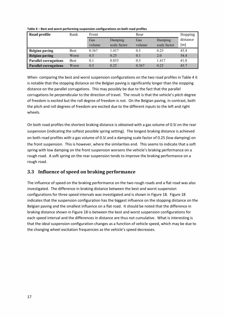
Table 4 – Best and worst performing suspension configurations on both road profiles

Road profile Rank Front Rear Stopping distance [m]

Gas volume

Damping scale factor

Gas volume

Damping scale factor

Belgian paving Best 0.367 1.417 0.5 0.25 45.4 Belgian paving Worst 0.5 0.25 0.1 2.0 54.4 Parallel corrugations Best 0.1 0.833 0.5 1.417 41.8 Parallel corrugations Worst 0.5 0.25 0.367 0.25 43.7

When comparing the best and worst suspension configurations on the two road profiles in Table 4 it is notable that the stopping distance on the Belgian paving is significantly longer than the stopping distance on the parallel corrugations. This may possibly be due to the fact that the parallel corrugations lie perpendicular to the direction of travel. The result is that the vehicle’s pitch degree of freedom is excited but the roll degree of freedom is not. On the Belgian paving, in contrast, both the pitch and roll degrees of freedom are excited due to the different inputs to the left and right wheels. On both road profiles the shortest braking distance is obtained with a gas volume of 0.5l on the rear suspension (indicating the softest possible spring setting). The longest braking distance is achieved on both road profiles with a gas volume of 0.5l and a damping scale factor of 0.25 (low damping) on the front suspension. This is however, where the similarities end. This seems to indicate that a soft spring with low damping on the front suspension worsens the vehicle’s braking performance on a rough road. A soft spring on the rear suspension tends to improve the braking performance on a rough road.

3.3 Influence of speed on braking performance

The influence of speed on the braking performance on the two rough roads and a flat road was also investigated. The difference in braking distance between the best and worst suspension configurations for three speed intervals was investigated and is shown in Figure 18. Figure 18 indicates that the suspension configuration has the biggest influence on the stopping distance on the Belgian paving and the smallest influence on a flat road. It should be noted that the difference in braking distance shown in Figure 18 is between the best and worst suspension configurations for each speed interval and the differences in distance are thus not cumulative. What is interesting is that the ideal suspension configuration changes as a function of vehicle speed, which may be due to the changing wheel excitation frequencies as the vehicle’s speed decreases.

17

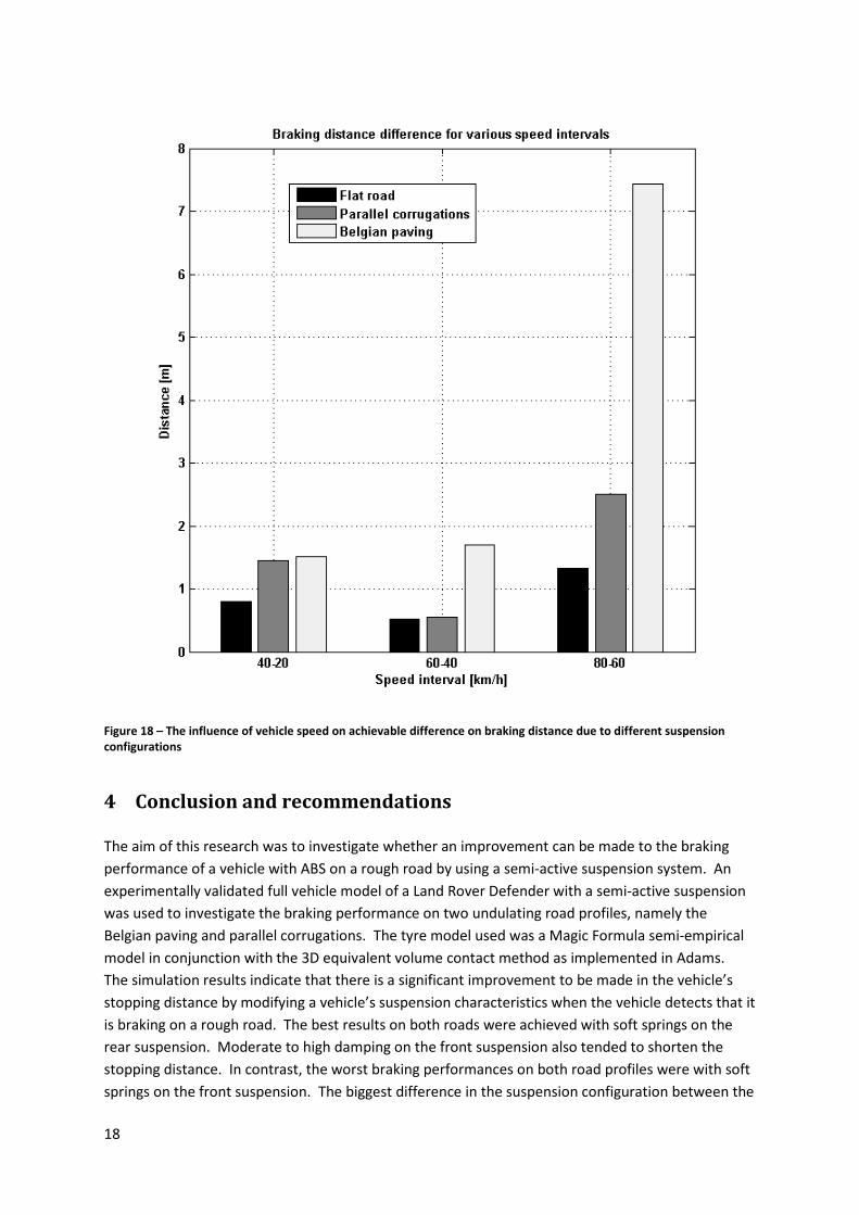
Figure 18 – The influence of vehicle speed on achievable difference on braking distance due to different suspension configurations

4 Conclusion and recommendations

The aim of this research was to investigate whether an improvement can be made to the braking performance of a vehicle with ABS on a rough road by using a semi-active suspension system. An experimentally validated full vehicle model of a Land Rover Defender with a semi-active suspension was used to investigate the braking performance on two undulating road profiles, namely the Belgian paving and parallel corrugations. The tyre model used was a Magic Formula semi-empirical model in conjunction with the 3D equivalent volume contact method as implemented in Adams. The simulation results indicate that there is a significant improvement to be made in the vehicle’s stopping distance by modifying a vehicle’s suspension characteristics when the vehicle detects that it is braking on a rough road. The best results on both roads were achieved with soft springs on the rear suspension. Moderate to high damping on the front suspension also tended to shorten the stopping distance. In contrast, the worst braking performances on both road profiles were with soft springs on the front suspension. The biggest difference in the suspension configuration between the

18

two road profiles was the damping in the rear suspension that gave the best results. Low damping in the rear on the Belgian paving gave the best result, while it gave the worst result on the parallel corrugations. Both these simulations used a soft spring in conjunction with the low damping. The vehicle’s speed also plays an important role in selecting the ideal configuration. While these results are promising, there is definite scope for further research. The most important is the refinement of the tyre model used. The Magic Formula approach may not be the ideal when transients play a big role, such as the case for ABS simulation, especially on an undulating road. Using an experimentally validated physics based approach, such as FTire, may lend more credibility to the simulations. The FTire tyre model may accurately capture the effect of the torsional dynamics of the tyre on the braking performance. Work has already begun on parameterising and validating an FTire model of the tyres used on the experimental vehicle. Furthermore the simulations should be repeated on the suspension tracks at Gerotek Test Facilities to experimentally confirm the improvement in the braking performance of the vehicle. Intelligently switching between suspension modes dependent on vehicle speed or wheel hop excitation may also be advantageous. As was shown by the simulation results, the braking performance can be improved, but the ideal suspension configuration depends to some extent on the roughness of the road. Using artificial intelligence techniques, such as stereovision, or investing in LIDAR technology, one may teach the vehicle to identify the road it is driving on and accordingly adjust the suspension to ensure optimum braking performance.

Acknowledgements

The authors wish to acknowledge the contributions made by the following:

1. Dr Valentin Ivanov, Dzmitry Savitski, Lucas Heidrich and Kristian Höpping from the Technische Universität Ilmenau, Ilmenau, Thuringia, Germany for their contribution of an ABS algorithm.

2. The financial assistance of the National Research Foundation (DAAD-NRF) towards this research is hereby acknowledged. Opinions expressed and conclusions arrived at, are those of the author and are not necessarily to be attributed to the DAAD-NRF.

Bibliography

[1] Gillespie, T. (1992). Fundamentals of Vehicle Dynamics. Warrendale, PA: Society of Automotive Engineers, Inc. [2] Breuer, B., & Bill, K. (2006). Brake Technology Handbook - 1st English Edition. Warrendale, PA: Society of Automotive Engineers, Inc. [3] Adcox, J., Ayalew, B., Rhyne, T., Cron, S., & Knauff, M. (2012). Interaction of Anti-lock Braking Systems with Tire Torsional Dynamics. Tire Science and Technology, TSTCA , Vol. 40 (No. 3), p. 171-185. [4] Hamersma, H., Els, P. B., Becker, C., Savitski, D., Heidrich, L., & Höpping, K. (4-7 November 2013). The effect of controllable suspension settings on the ABS braking performance of an off-road vehicle on rough terrain. 7th Americas Regional Conference of the ISTVS. Tampa, FL.

19

[5] Niemz, T., & Winner, H. (2006). Reduction of braking distance by control of active dampers. FISITA World Automotive Congress. Yokohama, Japan. [6] Theron, N., & Els, P. (2007). Modelling of a semi-active hydropneumatic spring-damper unit. International Journal of Vehicle Design , 45 (4), pp. 501-521. [7] Thoresson, M., Uys, P., Els, P., & Snyman, J. (2009). Efficient optimisation of a vehicle suspension system, using a gradient-based approximation method, Part 1: Mathematical modelling. Mathematical and Computer Modelling , 50 (9), pp. 1421-1436. [8] MSC Software Corporation. (n.d.). The Multibody Dynamics Simulation Solution. Retrieved July 18, 2013, from http://www.mscsoftware.com/product/adams [9] MathWorks. (n.d.). MATLAB: The Language of Technical Computing. Retrieved September 3, 2013, from http://www.mathworks.com/products/matlab [10] Savitski, D., Ivanov, V., Heidrich, L., Augsburg, K., & Pütz, T. (17-19 June 2013). Experimental investigation of braking dynamics of electric vehicle. Eurobrake Conference. Dresden, Germany. [11] Becker, C., & Els, P. (2014). Profiling of rough terrain. International Journal of Vehicle Design , 64 (2/3/4), pp. 240-261. [12] Gerotek Test Facilities. (n.d.). Retrieved from http://www.armscordi.com/SubSites/Gerotek1/Gerotek01_landing.asp [13] International Organization for Standardization. (1995). Mechanical Vibration - Road Surface Profiles - Reporting of Measured Data. [14] Budynas, R., & Nisbett, J. (2008). Shigley's Mechanical Engineering Design - Eigth Edition in SI Units. New York, NY: McGraw-Hill. [15] Bakker, E., Pacejka, H., & Lidner, L. (1989). A new tire model with an application in vehicle dynamics studies. Autotechnologies Conference and Exposition. Monte Carlo, Monaco. [16] Gipser, M. (2005). FTire: a physically based application-oriented tyre model for use with detailed MBS and finite-element suspension models. Vehicle System Dynamics: International Journal of Vehicle Mechanics and Mobility , Vol. 43 (Supplement 1), pp. 76-91. [17] Pacejka, H. (2005). Tyre and vehicle dynamics. Elsevier. [18] Stallmann, M., & Els, P. (2012). Validation of mathematical tyre models used in vertical dynamic simulations. 12th Regional Conference of the International Society for Terrain-Vehicle Systems. Pretoria, South Africa.

20