Blending regenerative and friction ABS braking of an ...

DF

Blending regenerative and friction ABSbraking of an electrified vehicle

Feasibility analysis of incorporating a regenerative braking sys-tem with friction brakes during an ABS intervention, a numeri-cal approach

Master’s thesis in Systems, Control and Mechatronics (MPSYS)

ERNAD MEHINAGICLEJLA CRNIC

Department of Electrical EngineeringCHALMERS UNIVERSITY OF TECHNOLOGYGothenburg, Sweden 2020

Blending regenerative and frictionABS braking of an electrified

vehicleFeasibility analysis of incorporating a regenerative brakingsystem with friction brakes during an ABS intervention, a

numerical approachMaster’s thesis in Systems, Control and Mechatronics (MPSYS)

ERNAD MEHINAGICLEJLA CRNIC

DF

Department of Electrical EngineeringDivision of Systems and Control

Chalmers University of TechnologyGothenburg, Sweden 2020

Blending regenerative and friction ABS braking ofan electrified vehicle

Feasibility analysis of incorporating a regenerative braking system with frictionbrakes during an ABS intervention, a numerical approachERNAD MEHINAGICLEJLA CRNIC

© ERNAD MEHINAGIC, LEJLA CRNIC 2020.

Supervisor: Staffan Johansson, Quintus Jalkler, Volvo CarsExaminer: Nikolce Murgovski, Department of Electrical Engineering

Master’s Thesis 2020: EENX30Department of Electrical EngineeringDivision of Systems and ControlChalmers University of TechnologySE-412 96 GothenburgTelephone +46 31 772 1000

Cover: Layout of Polestar 2 front axle [1].

Typeset in LATEX, template by David FriskPrinted by Chalmers ReproserviceGothenburg, Sweden 2020

iv

Blending friction and regenerative ABS braking of an electrified vehicleFeasibility analysis of incorporating a regenerative braking system with frictionbrakes during an ABS intervention, a numerical approachERNAD MEHINAGIC, LEJLA CRNICDepartment of Electrical EngineeringChalmers University of Technology

AbstractToday, most vehicles are developed with the aim of having an optimal energy ef-ficiency in order to reach sustainability goals. Major vehicle manufacturers sharethese values and are therefore trying to produce more efficient products by shiftingto an electrified propulsion system. Regenerative braking is used in electrified ve-hicles in order to convert kinetic energy into electric energy using an electric motor(EM). The part of the brake energy that is not recovered using regenerative brakingis covered by the friction brakes, thus could be considered as waste. Hence, it isbeneficial if regenerative braking could be optimized. There are certain load casesfor which regenerative braking could be used. One such load case is brake applica-tion that includes ABS intervention.

In this thesis an analysis was conducted, regarding the possibility to brake by merg-ing a frictional and regenerative brake system during an ABS intervention. Theintegration of a regenerative brake system with an ABS, requires a blended brakecontrol strategy. An optimal torque distribution between the operating brake sys-tems is crucial, if one desires to perform optimal brake blending. The primary aimof this thesis was to develop a torque distribution controller that enhances the brakeperformance during straight road driving. Two torque distribution controllers weredeveloped, one where maximal regenerative brake torque was applied and the otherwhere a regulated amount of regenerative brake torque was used. Both strategiesenhanced the braking performance by reducing the brake distance while still main-taining vehicle stability. Simulations show that a regulated amount of regenerativebrake torque was more effective in terms of reducing brake distance, whereas bymaximizing the regenerative brake torque gives a greater recuperation at the ex-pense of reducing the brake distance.

The safety aspect during an ABS intervention is of highest priority, implying thatreducing brake distance is of higher importance. The brake distance reduction wasmainly possible due to the fast response time from the EM used during regenerativebraking. The response time of the EM gave the braking a head start compared tothe conventional system using only friction brakes. Comfortability constraints ofthe EM can be removed in order to further decrease the ramp-up time and give theEM an even greater advantage compared to the frictional brake system. The resultsgained from the analysis conducted in this report, indicates that this type of brakeblending system gives the possibility to enhance brake performance.

v

Further research and development will enable brake blending during an ABS inter-vention in a real vehicle. The developed controllers still have room for improvementregarding performance and adaptability to altering driving scenarios, since the de-velopment was solely based on straight road driving. The current controllers havebeen substantiated using simulations only, in order to apply the controllers in avehicle future steps of validation have been determined.

Keywords: Brake blending, Torque distribution, Regenerative braking, Frictionbrake, EM, ABS, Brake distance.

vi

AcknowledgementsWe would like to give our supervisor at Volvo Cars, Quintus Jalkler, a special thanksfor helping us to acclimate to a new work environment and giving us guidance atthe start of the thesis.

We would like to give our greatest thanks to our supervisor at Volvo Cars, StaffanJohansson, for being very invested in helping us achieving our goals in this thesisand for always providing us with valuable knowledge both professionally and in life.This thesis would not have been the same without your help.

We also want to give a big thank you to our examiner at Chalmers, Nikolce Mur-govski, for giving us great feedback during our meetings and for guiding us forwardthrough this process. We are very grateful for all the academic support you providedus with.

Lastly we want to give a great thank you to our families and friends, for supportingus throughout this thesis and the rest of our academic journey.

Ernad Mehinagic & Lejla Crnic, Gothenburg, 09 2020

viii

Contents

List of Figures xiii

List of Tables xix

1 Introduction 11.1 Related work . . . . . . . . . . . . . . . . . . . . . . . . . . . . . . . 11.2 Objective . . . . . . . . . . . . . . . . . . . . . . . . . . . . . . . . . 21.3 Scope . . . . . . . . . . . . . . . . . . . . . . . . . . . . . . . . . . . 21.4 Delimitations . . . . . . . . . . . . . . . . . . . . . . . . . . . . . . . 3

2 Vehicle powertrain and braking system 52.1 Longitudinal vehicle dynamics . . . . . . . . . . . . . . . . . . . . . . 5

2.1.1 Single wheel model . . . . . . . . . . . . . . . . . . . . . . . . 72.1.2 Tire model (Friction estimator) . . . . . . . . . . . . . . . . . 8

2.2 Brake systems used during brake blending . . . . . . . . . . . . . . . 92.2.1 Friction brakes and braking by wire . . . . . . . . . . . . . . . 92.2.2 Regenerative brake system . . . . . . . . . . . . . . . . . . . . 10

2.3 The electric motor and its properties . . . . . . . . . . . . . . . . . . 112.3.1 Electric power storage system . . . . . . . . . . . . . . . . . . 12

2.4 Anti-lock braking system . . . . . . . . . . . . . . . . . . . . . . . . . 122.4.1 ABS-soft control strategy . . . . . . . . . . . . . . . . . . . . 122.4.2 Torque output of the ABS-soft model . . . . . . . . . . . . . . 13

2.5 Longitudinal dynamics during zero steering and constant heading . . 142.6 Brake blending during ABS . . . . . . . . . . . . . . . . . . . . . . . 15

3 Methods 173.1 Preliminary analysis regarding the implementation of a torque distri-

bution controller . . . . . . . . . . . . . . . . . . . . . . . . . . . . . 173.2 General torque distribution approach . . . . . . . . . . . . . . . . . . 173.3 Approach II, Brake Blending with maximal usage of the electric motor 20

3.3.1 Switch implementations necessary for a beneficial torque dis-tribution . . . . . . . . . . . . . . . . . . . . . . . . . . . . . . 21

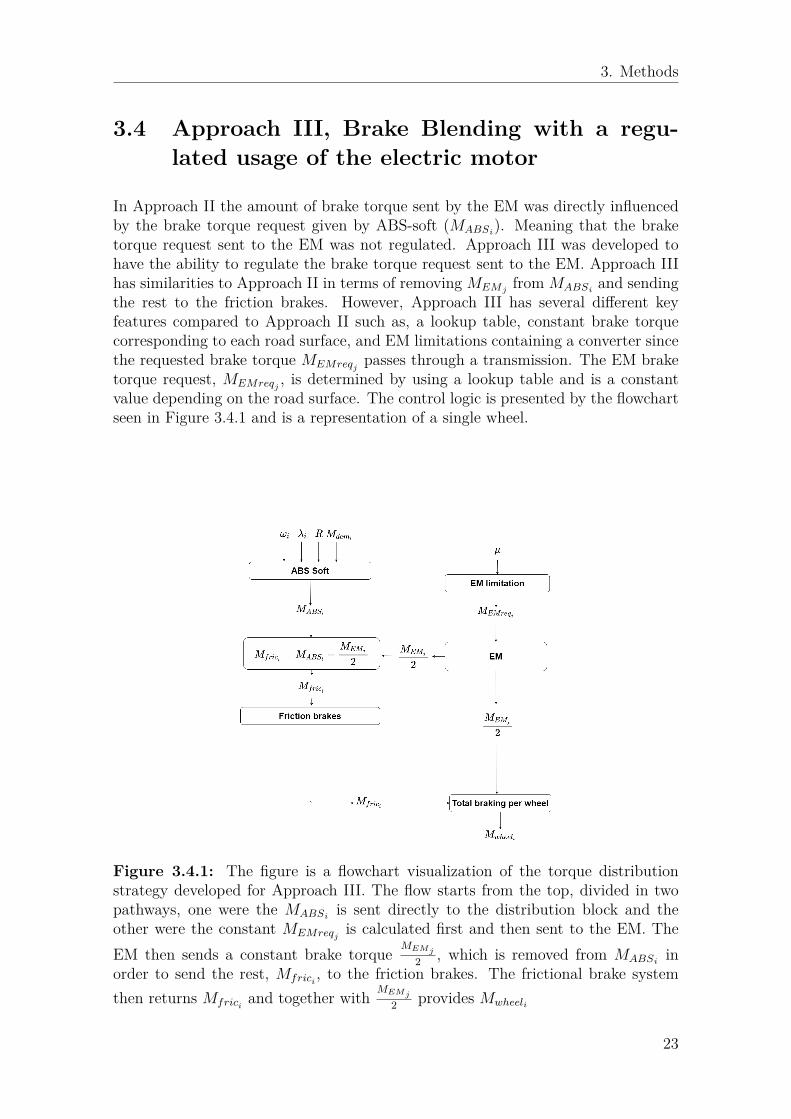
3.4 Approach III, Brake Blending with a regulated usage of the electricmotor . . . . . . . . . . . . . . . . . . . . . . . . . . . . . . . . . . . 233.4.1 Calculation of constant electric motor torque . . . . . . . . . . 24

3.4.1.1 Achieving a desired brake torque request using aextreme-value function . . . . . . . . . . . . . . . . . 24

xi

Contents

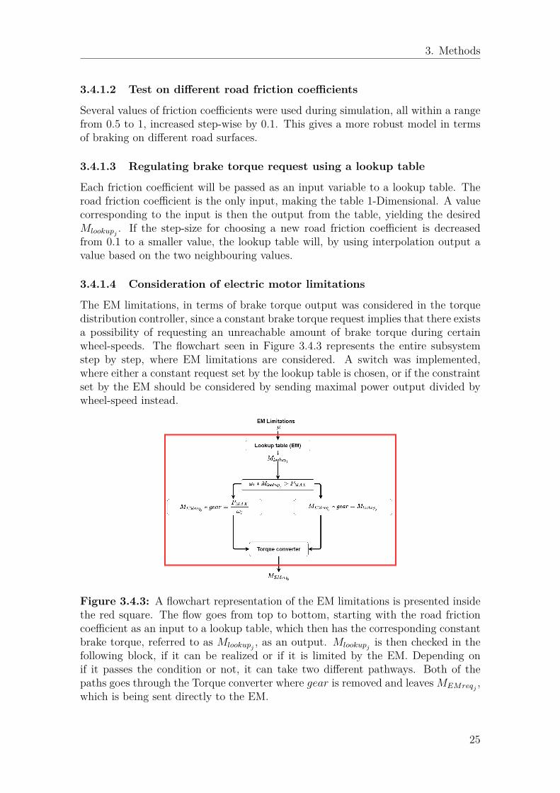
3.4.1.2 Test on different road friction coefficients . . . . . . . 253.4.1.3 Regulating brake torque request using a lookup table 253.4.1.4 Consideration of electric motor limitations . . . . . . 253.4.1.5 Torque conversion using a gear ratio . . . . . . . . . 26

3.5 Simulation tools used for model-construction and result provision . . 26

4 Results & Discussion 274.1 Approach II, Brake Blending with maximal usage of the electric motor 28

4.1.1 Comparison of brake torque when using brake blending andwhen not using brake blending . . . . . . . . . . . . . . . . . . 28

4.1.2 Comparison of slip when using brake blending and when notusing brake blending . . . . . . . . . . . . . . . . . . . . . . . 30

4.1.3 Deceleration when using brake blending and when not usingbrake blending . . . . . . . . . . . . . . . . . . . . . . . . . . 31

4.1.4 Comparison of velocity when using brake blending and whennot using brake blending . . . . . . . . . . . . . . . . . . . . . 31

4.1.5 Comparing brake distance when using brake blending andwhen not using brake blending . . . . . . . . . . . . . . . . . . 32

4.2 Approach III, Brake Blending with a regulated usage of the electricmotor . . . . . . . . . . . . . . . . . . . . . . . . . . . . . . . . . . . 344.2.1 Comparison of brake torque when using brake blending and

when not using brake blending . . . . . . . . . . . . . . . . . . 344.2.2 Comparison of slip when using brake blending and when not

using brake blending . . . . . . . . . . . . . . . . . . . . . . . 364.2.3 Comparison of deceleration when using brake blending and

when not using brake blending . . . . . . . . . . . . . . . . . . 374.2.4 Comparison of velocity when using brake blending and when

not using brake blending . . . . . . . . . . . . . . . . . . . . . 374.2.5 Comparing brake distance when using brake blending and

when not using brake blending . . . . . . . . . . . . . . . . . . 384.3 Design of experiments . . . . . . . . . . . . . . . . . . . . . . . . . . 40

5 Conclusion 43

6 Recommendation for future work 45

xii

List of Figures

1.3.1 Flowchart representation of the work flow in this thesis. The greyblocks are each one of the main parts of the work flow. The text inwhite describes how the work in each segment was conducted. Thecoloured circles describe how to transition into next state of the workflow. . . . . . . . . . . . . . . . . . . . . . . . . . . . . . . . . . . . . 3

2.0.1 Picture of the Polestar 2. . . . . . . . . . . . . . . . . . . . . . . . . . 52.1.1 Four wheel model representation. . . . . . . . . . . . . . . . . . . . . 62.1.2 Single wheel dynamics representation . . . . . . . . . . . . . . . . . . 72.1.3 Plot of road friction coefficient curve, where the x-axis is the slip ratio

λ in %, which ranges from values between 0% to 100%. The y-axisis the estimated road friction coefficient, µi, which has a maximumvalue of around 0.9 at a slip ratio of approximately 20%. . . . . . . . 9

2.2.1 The figure represents a part of the friction brake system. In the figurethe brake disc and the brake caliper are visible. . . . . . . . . . . . . 9

2.2.2 The hydraulic brake by wire brake system in Polestar 2. . . . . . . . 102.3.1 Plot of the torque output from the electric motor, which has a maxi-

mum value of 330 Nm. . . . . . . . . . . . . . . . . . . . . . . . . . . 112.4.1 This figure is visualization of how MABSi

is divided between eachfrictional brake for each wheel, during a brake application which in-cludes ABS intervention. The curve is plotted after 10s since the ABSintervention is initiated at 12s and terminated when the vehicle hasstopped at approximately 15s. . . . . . . . . . . . . . . . . . . . . . . 13

2.4.2 A representation of the pulsations (similar pulsations in all wheels)in the demanded torque for the front left wheel , caused by ABS-soft. The frequency is determined by how often the pressure has tobe maintained, reduced or released in order to perform slip/wheel-control. The pulsations are presented at a randomly selected timeinterval from the time period where these pulsations occur. . . . . . . 14

2.6.1 Control block diagram of the brake-blending system . . . . . . . . . . 15

xiii

List of Figures

3.2.1 The signal-path is from top to bottom. MABSi, is dependent on vari-

ables such as ωi, λi, R andMdemi. The ABS-soft model calculates the

requested torque MABSiand the EM provides the brake torque MEMj

2based on the brake torque requestMEMreqj

. MEMjis then subtracted

from MABSiand the remaining part of MABSi

is sent to the frictionalbrake system asMfrici

. The frictional brake system then sendsMfrici

and MEMj

2 is added to provide with Mwheeli . . . . . . . . . . . . . . . 18

3.2.2 Schematic view of complete brake system, including a visual repre-sentation of the brake torque distribution. . . . . . . . . . . . . . . . 19

3.3.1 Flowchart representation of Approach II. The signal-path is from topto bottom. The torque request from ABS-soft, MABSi

, is dependenton variables such as ωi, λi, R and Mdemi

. The ABS-soft model cal-culates the requested torque MABSi

and the EM provides the braketorque MEMj

2 based on the brake torque request MEMreqj. MEMj

isthen subtracted from MABSi

and the remaining part of MABSiis sent

to the frictional brake system as Mfrici. The frictional brake system

then sends Mfriciand MEMj

2 is added to provide with Mwheeli . . . . . 21

3.3.2 This figure visualizes the switch-logic, which starts from left by send-ing a constant value of 0 and the torque produced by the EM, MEMj

,to the block to its right, which sends the maximal value of the twoinputs. . . . . . . . . . . . . . . . . . . . . . . . . . . . . . . . . . . . 22

3.3.3 A visualization of the switch-logic constructed with the cause of pre-venting negative Mfrici

to be sent to the friction brakes. The logicstarts with the left side, where a constant value of zero and the differ-ence between MABSi

and MEMj, are used as inputs to the max block.

The max block then gives a positive value Mfricias an output. . . . . 22

3.3.4 This figure is a visual representation of the "system activator", wherethe three inputs to the left are, MEMreqj

(u1) , Brake Pressure (BP),(u2) and a constant value of zero (u3). These are the inputs to theswitch following to the right, where it gives an output of MEMreqj

ifBP is larger than 0, else a constant value of 0 is the output. . . . . . 22

3.4.1 The figure is a flowchart visualization of the torque distribution strat-egy developed for Approach III. The flow starts from the top, dividedin two pathways, one were the MABSi

is sent directly to the distribu-tion block and the other were the constantMEMreqj

is calculated firstand then sent to the EM. The EM then sends a constant brake torqueMEMj

2 , which is removed fromMABSiin order to send the rest, Mfrici

,to the friction brakes. The frictional brake system then returnsMfrici

and together with MEMj

2 provides Mwheeli . . . . . . . . . . . . . . . . 23

3.4.2 The figure is a representation of how the extreme-value function ischoosing Mlookupj

(red line) right before the oscillations seen in thedemanded torque(blue curve). . . . . . . . . . . . . . . . . . . . . . . 24

xiv

List of Figures

3.4.3 A flowchart representation of the EM limitations is presented insidethe red square. The flow goes from top to bottom, starting with theroad friction coefficient as an input to a lookup table, which then hasthe corresponding constant brake torque, referred to as Mlookupj

, asan output. Mlookupj

is then checked in the following block, if it canbe realized or if it is limited by the EM. Depending on if it passesthe condition or not, it can take two different pathways. Both of thepaths goes through the Torque converter where gear is removed andleaves MEMreqj

, which is being sent directly to the EM. . . . . . . . . 25

4.1.1 The figure is a representation of how Approach II performs duringTest Case 1 compared to Approach I, where each subplot representsone of the wheels. The curve is plotted after 10 s since the brakeapplication starts at time t ≥ 12 s and is terminated when the vehiclehas stopped at approximately 15 s. The one second pause intervalstarts at t ≈ 11 s and ends at t ≈ 12 s, the brake application thereforestarts at time t ≥ 12 s. . . . . . . . . . . . . . . . . . . . . . . . . . . 28

4.1.2 The figure is a representation of how Approach II performs duringTest Case 2 compared to Approach I, where each subplot representsone of the wheels. The curve is plotted after 10 s as the brake appli-cation starts at time t ≥ 11 s and is terminated when the vehicle hasstopped at approximately 14.5 s. . . . . . . . . . . . . . . . . . . . . . 29

4.1.3 A visual representation of the slip comparison between Approach Iand Approach II, for Test Case 1 (left plot) and Test Case 2 (rightplot). Both plots are a representation of the front left wheel. Thecurves are plotted after 10 s since the brake application starts at timet ≥ 12 s for Test Case 1 and t ≥ 11 s for Test Case 2. The onesecond pause interval for Test Case 1 starts at t ≈ 11 s and ends att ≈ 12 s, when the pause interval is completed the brake applicationsis initiated. The brake application for Test Case 1 is terminated whenthe vehicle has stopped at approximately 15 s and for Test Case 2 atapproximately 14 s. . . . . . . . . . . . . . . . . . . . . . . . . . . . . 30

4.1.4 The figure is a representation of the resulting vehicle decelerationcomparison, between Approach I and Approach II, during Test Case1 (left plot) and Test Case 2 (right plot). The vehicle did not start toaccelerate (positive valued curve) untilt ≥ 2 s for Test Case 1 and 2.The curves are plotted after 10 s since the brake applications startsat time t ≥ 12 s for Test Case 1 and t ≥ 11 s for Test Case 2. The onesecond pause interval for Test Case 1 starts at t ≈ 11 s and ends att ≈ 12 s, when the pause interval is completed the brake applicationis initiated. The brake application for Test Case 1 is terminated whenthe vehicle has stopped at approximately 15 s and for Test Case 2 atapproximately 14 s.. . . . . . . . . . . . . . . . . . . . . . . . . . . . . 31

xv

List of Figures

4.1.5 The figure is a representation of the resulting vehicle velocity whenusing Approach I and II, during Test Case 1 (left plot) and Test Case2 (right plot). The vehicle does not start to accelerate until t ≥ 2 sfor Test Case 1 and 2. For Test Case 1 the one second pause intervalstarts at t ≈ 11 s and ends at t ≈ 12 s , when the pause interval iscompleted the brake applications starts at time t ≥ 12 s . In Test Case2 the brake application is initiated at t ≥ 11 s . The brake applicationinitiation is marked in both plots with a grey square, where it can beseen that velocity between Approach I and II differs for both cases. . 32

4.1.6 The figure is a representation of the resulting vehicle brake distancewhen using Approach I and II, during Test Case 1 (left plot) and TestCase 2 (right plot). The brake application starts at time t ≥ 12 s forTest Case 1. In Test Case 2 the brake application is initiated att ≥ 11 s . . . . . . . . . . . . . . . . . . . . . . . . . . . . . . . . . . . 33

4.1.7 The figure is a representation of the brake distance difference betweenApproach I and Approach II for Test Case 1 and 2. The x-axis repre-sents the time that the car is braking and the y-axis represents howbig the difference is between the brake distance for Approach I andApproach II. . . . . . . . . . . . . . . . . . . . . . . . . . . . . . . . . 33

4.2.1 The figure is a representation of how Approach III performs duringTest Case 1 compared to Approach I, where each subplot representsone of the wheels. The one second pause interval is starting at t ≈ 11 sand ending at t ≈ 12 s , when the pause interval is completed thebrake applications starts at time t ≥ 12 s . . . . . . . . . . . . . . . . 34

4.2.2 The figure is a representation of how Approach III performs duringTest Case 2 compared to Approach I, where each subplot representsone of the wheels. The brake applications starts at time t ≈ 11 s . . . 35

4.2.3 A visual representation of the slip comparison between Approach Iand Approach III, for Test Case 1 (left plot) and Test Case 2 (rightplot). Both plots are a representation of the front left wheel. Thebrake application ends at approximately 15.5 s for Test Case 1 andaround 14.5 s for Test Case 2. . . . . . . . . . . . . . . . . . . . . . . 36

4.2.4 The figure is a representation of the resulting vehicle decelerationcomparison, between Approach I and Approach III, during Test Case1 (left plot) and Test Case 2 (right plot). The vehicle does not startto accelerate (positive valued curve) until t ≥ 2 s for Test Case 1and 2. For Test Case 1 the one second pause interval is starts att ≈ 11 s and ends at t ≈ 12 s, when the pause interval is completedthe brake application starts at time t ≥ 12 s. In Test Case 2 thebrake application is initiated at t ≥ 11 s. For both Test Case 1 and2 a positive spike at 1g-force is visible at around 15 s , meaning thatthe brake application is terminated and the vehicle is no longer inmotion (this is not relevant and thus not considered in the results). . 37

xvi

List of Figures

4.2.5 The figure is a representation of the resulting vehicle velocity whenusing Approach I and III, during Test Case 1 (left plot) and Test Case2 (right plot). The vehicle does not start to accelerate until t ≥ 2 sfor Test Case 1 and 2. For Test Case 1 the one second pause intervalstarts at t ≈ 11 s and ends at t ≈ 12 s, when the pause interval iscompleted the brake applications starts at time t ≥ 12 s. In Test Case2 the brake application is initiated at t ≥ 11 s. The brake applicationinitiation is marked in both plots with a grey square, where it can beseen that velocity between Approach I and III differs for both cases. . 38

4.2.6 The figure is a representation of the resulting vehicle braking distancewhen using Approach I and III, during Test Case 1 (left plot) and TestCase 2 (right plot). The brake application starts at time t ≥ 12 s forTest Case 1. In Test Case 2 the brake application is initiated at t ≥ 11 s. 39

4.2.7 The figure is a representation of the brake distance difference betweenApproach I and Approach III for Test Case 1 and 2. The x-axisrepresents the time that the car is braking and the y-axis representshow big the difference is between the brake distance for Approach Iand Approach III. . . . . . . . . . . . . . . . . . . . . . . . . . . . . . 39

4.3.1 The figure represents a DOE where the different brake distance resultsfor each Approach is visible. . . . . . . . . . . . . . . . . . . . . . . 40

4.3.2 The Figure represents what happens with one of the wheels whenApproach II performs poorly on a road friction coefficient of 0.5. Itcan be seen from the red EM curve how the electric motor is tryingto pulsate but has a slow ramp-up, since the ramp-up time is limitedby a comfort constraint. . . . . . . . . . . . . . . . . . . . . . . . . . 41

4.3.3 The Figure represents what happens with one of the wheels whenApproach III performs well on low road friction coefficient. It can beobserved that the pulsations are handled by the friction brakes andnot by the EM as they are in Approach II. . . . . . . . . . . . . . . . 41

xvii

List of Figures

xviii

List of Tables

2.1 A table with values of constants A (peak value of the road friction),B (road friction curve shape) and C (road friction curve differencebetween the maximum value and the value at λi = 1). The values ofthese constants are determined by the condition of having dry asphalt. 8

xix

List of Tables

xx

1Introduction

Today, the majority of vehicles are developed with the aim of having an optimalenergy efficiency in order to reach sustainability goals. Major vehicle manufacturersshare these values and are therefore trying to produce more efficient products byshifting to electrified propulsion systems [2]. An example of electrified propulsionis Battery Electric Vehicles (BEVs), which is a technology that is looked upon as apromising solution to more sustainable transportation, as it has the potential to re-place vehicles that are powered by fossil fuels [2]. The electrified powertrain systemenables new functions and possibilities, alongside being more efficient than tradi-tional vehicles, they allow for the recuperation of mechanical energy into electricalenergy also known as regenerative braking [3, 4].

Regenerative braking is used in cars in order to convert kinetic energy into electricenergy using an electric motor and a battery. Electric vehicles often use regenera-tive braking combined with friction brakes, which is also known as brake blending.Research and use of brake blending is focused on conventional deceleration levels [5].However, brake blending is not utilized in emergency braking scenarios, when theAnti-lock Braking System (ABS) is activated. As mentioned in [5, 6], when ABS isactivated the regenerative braking torque will be removed, which means that onlythe friction brakes will operate, to prevent possible wheel lock and stability issues.This is due to the fact that poorly handled regenerative braking can result in vehicleinstability, reduce handling capability and decrease braking performance [7]. An-other issue with regenerative braking is that limited electric motor power will causedifficulties at a higher deceleration rate, as more power is required to slow down thevehicle down than is available [8].

1.1 Related workEarlier research [9, 10, 11, 12] has focused on determining the possibilities of inte-grating ABS with regenerative braking, without decreasing brake performance. Theresearchers in [9] have shown that it is possible to integrate and recover a signifi-cant amount of braking energy. However their research has been performed on abicycle wheel which leaves the question of how realistic the results are for a carwheel. This question has been addressed by researchers in [10] which have testedtheir regenerative braking based ABS controller, in both simulation and on a real

1

1. Introduction

vehicle. Their results show an improved energy recovery during ABS-situations by60% in simulation and 40% in real vehicle test [10].

Similar research has been made in [11, 12]. Brake blending control, where regener-ative braking is merged with a frictional brake system, has been studied in orderto attempt to understand the capabilities of the regenerative braking system. Theenergy recovery limits have been investigated along with how these limits can af-fect the stability or maneuverability of the vehicle at hand. Electric motors wereused for a certain fraction of the requested brake torque, while the remaining partwas handled by the friction brakes. These simulations were performed on a hybridvehicle with one electric motor on the rear axle. There were two proposed torquedistribution control strategies, where the results from both imply that rear axleregenerative braking can be effective [11, 12].

As can be seen from above, there were several studies that suggest that brake blend-ing is possible and beneficial and that there are several approaches to the problem.Therefore the main challenges lie with the smooth interaction between friction andregenerative brakes, along with proper torque distribution in brake blending systems,for these systems to be feasible.

1.2 ObjectiveThe objective of this thesis is to develop a torque distribution controller, that splitsbrake torque between a regenerative and frictional braking system, during ABSintervention. There are two main research questions that need to be answered inorder to be able to achieve the project goals:

1. How will the torque split affect the brake distance?

2. How much regenerative braking can be effectively applied?

1.3 ScopeThe project began with finding a suitable controller for a car that accelerates to130 km/h and proceeds to decelerate as quickly as possible. This scenario can causewheel lock and loss of traction which activates the ABS function. The main focusof the project was to develop a control model that will make an optimal torquedistribution between friction brakes and regenerative braking while ABS is active.

The controller could not be developed without necessary preparations. Figure 1.3.1is a visual representation of the necessary steps that were taken in order to developa torque distribution controller.

2

1. Introduction

Figure 1.3.1: Flowchart representation of the work flow in this thesis. The greyblocks are each one of the main parts of the work flow. The text in white describeshow the work in each segment was conducted. The coloured circles describe how totransition into next state of the work flow.

1.4 DelimitationsThe following points are the delimitations set in this project

• It was assumed that the car drives on a straight road and that the steeringwill always keep the car in a straight line, meaning no lateral or horizontaldisplacements were considered.

• The road friction coefficient was selected relatively low in order to easily trig-ger ABS and was altered to see how the control models perform on differentsurfaces, however only two were used for the controller evaluation.

• The battery state of charge was considered as constant, meaning that batterylimitations are not considered. Temperature influence was not considered, e.gthat from high battery temperature that can affect the possibility of regener-ation or the effects of the electric motor during high operating temperatures.

• Parameters such as the operating efficiency and the conversion efficiency forconverting into regenerative braking will not be considered.

• The simulations are performed solely on one type of vehicle, the Polestar 2and the brake blending is tested with one ABS model, ABS-Soft provided byIPG [13].

3

1. Introduction

4

2Vehicle powertrain and braking

system

The vehicle used in this study is the premium all-electric 5-door all-wheel drive(AWD) Polestar 2. This car was developed based on Volvo Car Group’s adaptableCompact Modular Architecture platform (CMA)[1]. The Polestar 2 falls into thecategory of a battery electric vehicle (BEV). The body-shape of the Polestar 2 is a"fastback" shape, very similar to a sedan body-shape, except that the rear windowand boot door open as one unit[1].

Figure 2.0.1: Picture of the Polestar 2.

2.1 Longitudinal vehicle dynamicsThis aim of the section is to provide the reader with some basics in longitudinaldynamics, in order to give a better understanding how certain forces are connected.The dynamics are primarily presented for the entire vehicle (4 wheels) and is then

5

2. Vehicle powertrain and braking system

narrowed down to single wheel dynamics. The ABS controller used in this projectis based on single wheel dynamics and the torque distribution controller will workaccordingly.

Figure 2.1.1: Four wheel model representation.

This project has only considered longitudinal movements and no lateral displace-ments. The longitudinal forces acting on the vehicle are expressed in the equationsbelow and are also visible in Figure 2.1.1. Even though no turning motions areconsidered, the vehicle yaw rate (ψ) and the turning angle rate of the wheel (δ) arerepresented in the figure and in equations. This is done to show how longitudinalforces are affected by lateral movements.

With the help of Newtons second law a force balance along the longitudinal axis canbe represented as

mx = myψ +∑

Fxi, i = {fl, fr, rl, rr} (2.1)

where m is the vehicle mass, x is the longitudinal acceleration, Fxiis the tire force

in vehicle body frame. The subscript i indicates what wheel is referred to, where flstands for front left wheel, fr front right wheel, rl rear left wheel and rr rear rightwheel.

The tire force mapping from wheel to vehicle body frame and can be represented as

Fxi= µi(λi)FNi

cos(δj), j = {f, r} (2.2)

where λi is longitudinal slip ratio, µi is road friction coefficient and FNiis the normal

force. Subscript j is indicating which axle a variable belongs to, and it works asfollows, f (front) and r (rear). The longitudinal wheel velocity, vli , defined in thetire frame, is expressed as

vli = vxicos(δj) (2.3)

6


where vxiis the longitudinal wheel speed in the vehicle frame. This speed is related

to the vehicle speed,vxfr

= x+ cψ (2.4)vxfl

= x− cψ (2.5)vxrr = x+ cψ (2.6)vxrl

= x− cψ (2.7)where c is the length between the center of the wheel and the center of the respectiveaxle. Representation of signals associated to each wheel can be seen in equations(2.4) to (2.7).

2.1.1 Single wheel modelFigure 2.1.2 is a visual representation of the single wheel model, used in order toprovide the reader with a clearer view of the single wheel dynamics.

Figure 2.1.2: Single wheel dynamics representation

In this project the vehicle is assumed to have a straight motion, meaning that nolateral forces are considered. This will give the system one degree of freedom (DOF)on each wheel. The model is describing the elementary dynamic properties of thesystem [14], and its equation of motion is described as

Jiωi = −FxiR +Mwheeli − bdωi. (2.8)

In equation (2.8), Mwheeli is the brake torque provided for each wheel, ωi is theangular speed of the wheel, Ji is the wheel rotational moment of inertia, R is thewheel radius, bd is a damping factor.

Equation (2.9) is a representation of how the two different brake systems are pro-viding with the brake torque applied on each wheel.

Mwheeli = Mfrici+MEMj

2 (2.9)

7


Here, Mfrici≤ 0 is the braking torque provided by the friction brakes for each wheel

and MEMjis the torque provided by the EM on axle j. Equation (2.10) is then a

representation of each wheel.

Jiωi =

Jfr ˙ωfr = −FxfrR + Mfricfr

+MEMf

2 − bdωfr, i = fr

Jfl ˙ωfl = −FxflR + Mfricfl

+MEMf

2 − bdωfl, i = fl

Jrr ˙ωrr = −Fxrr R + Mfricrr + MEMr2 − bdωrr, i = rr

Jrlωrl = −FxrlR + Mfricrl

+ MEMr2 − bdωrl, i = rl

(2.10)

The EM torque is equally distributed between the left and right wheel. Duringbraking, when the longitudinal wheel speed is greater than or equal to its angularspeed, i.e. vli ≥ Rωi, the wheel may start to slip. Then, the longitudinal wheel slipλi is derived as

λi = Rωi − vlivli

, if vli ≥ Rωi, vli 6= 0. (2.11)

2.1.2 Tire model (Friction estimator)In this thesis, the Burckhardt model will be used, as it is optimized for analyti-cal determinations while maintaining accuracy within the delimitations set for theproject while estimating the road friction coefficient. Hence, the longitudinal frictioncoefficient estimator is as follows

µi(λi) = A(1− e−Bλi − Cλi) (2.12)

A (peak value of the road friction), B (road friction curve shape) and C (roadfriction curve difference between the maximum value and the value at λi = 1) areconstants that changes depending on the road surface. Dry asphalt is the conditionwhich will be used, where the values of each coefficient can be seen in Table 2.1[15].

Estimator coefficientsCondition A B CDry asphalt 1.029 17.16 0.523

Table 2.1: A table with values of constants A (peak value of the road friction), B(road friction curve shape) and C (road friction curve difference between the maxi-mum value and the value at λi = 1). The values of these constants are determinedby the condition of having dry asphalt.

The slip ratio-friction coefficient curve has been plotted with the help of Matlab andis visible below in Figure 2.1.3.

8


Figure 2.1.3: Plot of road friction coefficient curve, where the x-axis is the slipratio λ in %, which ranges from values between 0% to 100%. The y-axis is theestimated road friction coefficient, µi, which has a maximum value of around 0.9 ata slip ratio of approximately 20%.

2.2 Brake systems used during brake blendingThe entire brake system consists of two types of systems, a frictional brake systemand a regenerative brake system. The frictional brake system is not modelled withinthis work, since it is provided by IPG’s CarMaker. CarMaker, along with Simulink isused to model the torque distribution controller. The powertrain model is providedby Volvo and the ABS model is provided by IPG. The goal is to allocate this braketorque request between the two different brake systems.

2.2.1 Friction brakes and braking by wire

Figure 2.2.1: The figure represents a part of the friction brake system. In thefigure the brake disc and the brake caliper are visible.

9


Friction brakes are mechanical devices which are used to decelerate the vehicle byconverting hydraulic pressure to clamp force, thus creating brake torque. Frictionbrakes are also known as hydraulic brakes since they use fluid to create a brakepressure. The hydraulic brakes are divided in two categories, brake by wire orfull hydraulic. Full hydraulic implies brake system in the car uses brake fluid tomechanically brake the wheels, while brake by wire controls the hydraulic pressureat the wheel using electrical means.

The brake by wire system is mechanically decoupling the brake pedal from thehydraulic brake system, which is increasing the flexibility of the brake torque mod-ulation. Brake by wire fits well with vehicles that use frictional brakes and regen-erative braking system in cooperation. The brake by wire system can achieve idealbrake torque distribution by modulating the brake torques between rear and frontaxle. The brake torque allocation has to be taken into consideration when trying toachieve an effective regenerative system and assure that no wheel lock occurs [5].

2.2.2 Regenerative brake system

Figure 2.2.2: The hydraulic brake by wire brake system in Polestar 2.

A regenerative braking technology can be seen in various electric vehicles today,where the primary goals are to have a safe brake system and to recuperate as muchenergy as possible. Improvements towards a cleaner energy consumption is neededin order to improve environmental aspects. These improvements could be to increasethe efficiency of certain systems. There are studies which show that approximatelyone third to one half of the power plant energy is used when braking. It is where theregenerative braking system comes into play, since it offers the possibility to convertthe kinetic energy, which would otherwise be converted into heat, into electric energyand thereby improve fuel economy.[5]

As mentioned above, most electric vehicles use regenerative braking, however, in or-der to assure that the deceleration process meets the requirements, frictional brakesare applied. This type of system is often referred to as a "blended" brake system.

10


A blended brake system is used (frictional brake system and regenerative brake sys-tem) and it is therefore important that both systems are well integrated with oneanother. Hence, the structure of both systems are of importance for when a con-trol strategy is considered. The control strategy has to be effective and based onan appropriate brake system, to achieve good results. The brake torque from theregenerative brake system and the frictional brake system have to be synchronizedto fulfill the braking request from the driver and to optimize the regeneration. Thebrake torque provided from the electric motor needs to be regulated in order to fitthe variations in torque from the frictional brake system [5].

2.3 The electric motor and its propertiesThe electric powertrain of the Polestar 2 consists of two 150 kW/330 Nm electricmotors, where each axle consists of one electric motor (EM). The EM is a permanentmagnet brushless DC motor, which is commonly used in electric vehicles due to itshigh efficiency, low wear and high specific power output [16].

Figure 2.3.1: Plot of the torque output from the electric motor, which has amaximum value of 330 Nm.

The EM will have a constant peak output value from zero to a specific EM speed.Then at EM speeds which reach values outside of this interval the torque outputwill gradually start to decrease. This can be seen in Figure 2.3.1 , where the torquestarts to dip. Mathematically, the torque limit can be expressed as

MEMj min(ωEMj(ωi)) ≤MEMj

≤MEMj max(ωEMj(ωi)) (2.13)

where MEMj min and MEMj max are nonlinear functions, typically given as lookuptables. The EM speed is directly related to the speed of the wheels through thedifferential gears.

The EM functions as an actuator during drive mode, while it is used as a generatorduring regenerative braking mode. During drive mode, the torque can be estimated

11


with the help of the first order equation seen below [17]

MEMj=MEMreqj

−MEMj

τEM(2.14)

where MEMreqjis the requested electric motor torque and τEM is the EM time

constant.

2.3.1 Electric power storage systemThe battery is the electrical motors power source. A battery model is provided byVolvo, and is used for this masters’ thesis. The battery State of Charge (SOC) willbe set to a constant value, as mentioned in the delimitation section. Hence, nolimiting factors imposed by the battery will be considered.

2.4 Anti-lock braking systemThe purpose of the ABS is to achieve the shortest longitudinal stopping distancewhile maintaining vehicle stability during deceleration. This is achieved by imple-menting a feedback control for the slip, which can control the slip at the point wheremaximum brake torque is employed on the wheel. The ABS model used in this thesisis referred to as ABS-soft. The ABS-soft model is based on single wheel dynamics,where it provides each wheel with a brake torque request. This section will providewith information about the ABS-soft model and its functionalities.

2.4.1 ABS-soft control strategyThe control strategy is based on a trigger criterion which combines wheel decelera-tion and slip control. This is done with the help of weighting factors, the expressionseen in equation 2.14 is a representation of the control strategy [18].

Si = Kωωi +Kλλi (2.15)where Kω and Kλ are weighting factors.

The desired value of Si is between 0.15 − 0.2, this is the region where the optimaladhesion utilization is achieved. The model is built such that the brake pressureis reduced, released or maintained, in order to maintain Si in the desired region.The ABS-soft model contains a subsystem where the driver brake input is convertedin order to perform slip control. The driver is giving brake torque input to themodel when full braking is applied. A filter is constructed, where a torque updateis performed. The brake torque driver input is sent to the filter as pulsations be-tween zero and max. The pulsations are decided by either reducing or releasing thepressure. The second input to the filter is a constant value, which is sent when thepressure should be maintained. The ABS-soft output for each wheel is described inthe following equation

MABSi= fABS(Mdemi

, Si(ωi, λi(ωi))) (2.16)

12


where Mdemiis the brake torque demanded at wheel i, MABSi

is brake torque re-quested by the ABS-soft model.

The goal of this project is to split the torque request by the ABS controller intofriction and regenerative braking, i.e.

MABSi= Mfrici

+MEMj

2 (2.17)

where Mfriciis the brake torque request sent to the frictional brake system. Since

the frictional brake system has no dynamics modelled it yields that the requestis equal to the actual brake torque provided by the frictional brake system. Theright-hand side terms in equation (2.17) are identical to the right-hand side termsin equation (2.10), giving that

MABSi= Mwheeli . (2.18)

2.4.2 Torque output of the ABS-soft modelFigure 2.4.1 and 2.4.2 are a representation of theMABSi

determined by the ABS-softmodel. These torques will be fundamental to construct a proper torque distributioncontroller. From Figure 2.4.1 it can be seen that the ABS intervention is initiated at12s and terminated when the vehicle has stopped at approximately 15s. The braketorque then transitions from the ABS-soft request of 3000 Nm to full braking witha brake torque of 6000 Nm, which explains the peak at 16s.

10 12 14 16

Time[s]

0

2000

4000

6000

To

rqu

e[N

m]

Front left wheel

Friction Brakes

10 12 14 16

Time[s]

0

2000

4000

6000

To

rqu

e[N

m]

Front right wheel

Friction Brakes

10 12 14 16

Time[s]

0

2000

4000

6000

To

rqu

e[N

m]

Rear left wheel

Friction Brakes

10 12 14 16

Time[s]

0

2000

4000

6000

To

rqu

e[N

m]

Rear right wheel

Friction Brakes

Figure 2.4.1: This figure is visualization of how MABSiis divided between each

frictional brake for each wheel, during a brake application which includes ABS in-tervention. The curve is plotted after 10s since the ABS intervention is initiated at12s and terminated when the vehicle has stopped at approximately 15s.

13


13 13.5 14 14.5 15

Time[s]

3195

3200

3205

3210

3215

3220

3225

3230

3235

3240

3245

3250

Torq

ue[N

m]

Front left wheel

Friction Brakes

Figure 2.4.2: A representation of the pulsations (similar pulsations in all wheels)in the demanded torque for the front left wheel , caused by ABS-soft. The frequencyis determined by how often the pressure has to be maintained, reduced or releasedin order to perform slip/wheel-control. The pulsations are presented at a randomlyselected time interval from the time period where these pulsations occur.

2.5 Longitudinal dynamics during zero steeringand constant heading

In this work a study of a simplified scenario where the vehicle yaw rate, yaw angleand steering angle are zero was performed, i.e. ψ = 0, ψ = 0, δ = 0. Then, it holds

Fxi= Fli = µi(λi(ωi, v))FNi

(2.19)vli = vxi

= x = v (2.20)

where v is the vehicle speed and the function λ for computing longitudinal slip hasbeen defined in (2.11). The vehicle equations of motion then simplify to

v = 1m

∑µi(λi(ωi, v))FNi

(2.21)

ωi = 1Ji

(−(µi(λi(ωi, v))FNi)R +MABSi

− bdωi) (2.22)

MEMj=MEM_reqj

−MEMj

τEM. (2.23)

Here, v, ωi andMEMjare states in the system,MEMreqj

is the controllable input andMABSi

and FNiare uncontrollable inputs, i.e. they are decided by other controllers

or system dynamics. Recall that the EM torque is bounded

MEMj min(ωEMj(ωi)) ≤MEMj

≤MEMj max(ωEMj(ωi)) (2.24)

as well as the requested EM torqueMEMj

2 ≥MABSi(2.25)

14


which derives from the fact that the friction torque is nonpositive.

Notice that, if MEMjis decided, then the wheel friction torque is readily available

from (2.17).

2.6 Brake blending during ABSBrake blending in today’s vehicle is not active during an ABS situation, this is dueto not having any unforeseen issues. Figure 2.6.1 shows how brake-blending works,however during ABS MEMreqj

is zero. Mdem is divided between front and rear axle,70%/30%. The ABS block calculates the torque that is actually needed if the carstarts to slip in order to prevent the wheels from locking. Torque split divides thetorque from the ABS between the EM and the friction brakes. At every wheel thereis a speed sensor that calculates the wheel speed and sends it back as a feedback tothe controller. The car velocity is estimated as well in order to compare it to thewheel speed and calculate the slip.

Figure 2.6.1: Control block diagram of the brake-blending system

15


16

3Methods

3.1 Preliminary analysis regarding the implemen-tation of a torque distribution controller

As the Simulink model provided by Volvo is very extensive, this model was studiedto understand how to implement the control logic. It contains the powertrain ofPolestar 2. The friction brakes is a part of CarMaker, meaning that a connectionbetween the model and CarMaker was needed to perform analysis involving brakeblending. The brake blending controller was implemented inside of the CarMakerblocks. Hence, the earlier mentioned connection is between the plant in the Simulinkmodel and the control logic. The torque signals from the EM are used as an inputand the brake request from the control logic to the EM is the output, meaning thatit is a closed loop.

Proper subsystem connections within the model are of great importance, while for anextensive model the complexity of making valid connections increases. This impliedthat a lot of signal routing was required. An example of why proper connections areimportant, is when the EM brake torque request has to be sent to the transmission inorder to receive a correct amount of brake torque. If the signal is incorrectly routedpast the transmission, a too small amount of brake torque will be provided by the EMsince a gear is used in the transmission to produce more brake torque. Connectionslike the one mentioned in the example have all been taken into consideration andthereby provided for the prerequisites required for constructing a torque distributioncontroller.

3.2 General torque distribution approachAs mentioned previously (see Section 2.2.1), an electric vehicle that uses brake blend-ing, is often equipped with a brake by wire system in order to achieve ideal braketorque distribution. Brake torque distribution affects the efficiency and stabilityof the regenerative braking system, meaning that it is of utmost importance. Theallocation between rear and front brake torque distribution will also have an impacton the stopping distance, vehicle directional control, the durability and thermal loadon the brakes. The stopping distance is improved by optimizing the use of adhe-

17

3. Methods

sion, while over-braking an axle can cause steering and stability problems. Lastlythe regenerative braking predominantly affects the strongest braked axle in termsof brake wear and thermal load [11].

Figure 3.2.1: The signal-path is from top to bottom. MABSi, is dependent on

variables such as ωi, λi, R and Mdemi. The ABS-soft model calculates the requested

torque MABSiand the EM provides the brake torque MEMj

2 based on the braketorque request MEMreqj

. MEMjis then subtracted from MABSi

and the remainingpart of MABSi

is sent to the frictional brake system as Mfrici. The frictional brake

system then sends Mfriciand MEMj

2 is added to provide with Mwheeli .

The flowchart seen in Figure 3.2.1, visualizes how brake torque requests are handledby ABS-soft and distributed between the EM and friction brakes, where all of thebrake torques in Chapter 3 are considered as positive. It can be seen how the ABS-soft requested torque for each wheel, MABSi

, is dependent on variables such as ωi,λi, R and Mdemi

. The ABS-soft model calculates the requested torque MABSiand

the EM brake torque MEMj

2 is then subtracted fromMABSi. The remainder ofMABSi

is then sent to the frictional brake system as Mfrici, this is derived with the help of

equation (3.1). The frictional brake system then provides Mfriciand together with

MEMj

2 adds up to Mwheeli . The brake request sent to the EM, MEMreqj, will later on

18

3. Methods

Figure 3.2.2: Schematic view of complete brake system, including a visual repre-sentation of the brake torque distribution.

be sent in two different ways, seen in sections 3.3− 3.4, where two different controlmethods are presented.

A regenerative brake system should be able to reach the goal of the required braketorque, while recuperating as much energy as possible. The system needs to outputthe right amount of braking torque in order to meet the requirements during decel-eration. As mentioned before, brake torque for each wheel needs to be distributedproperly in order to maintain vehicle stability. When these two requirements arefulfilled, then energy regeneration can be optimized to recuperate as much energyas possible. [11].

Figure 3.2.2 is a visualization of the entire brake system and brake torque distribu-tion.

The total requested brake torque is provided by the electric motor and the frictionalbrakes, the expression seen in equation (3.1) shows how the torque from the electric

19

3. Methods

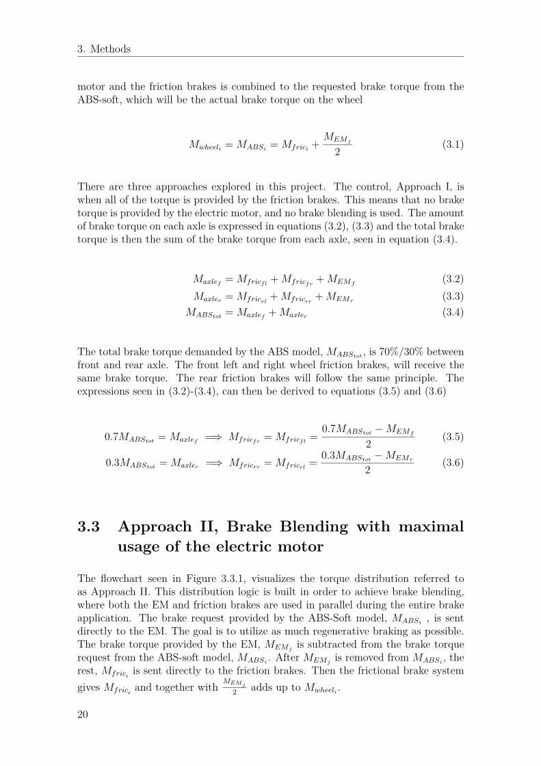
motor and the friction brakes is combined to the requested brake torque from theABS-soft, which will be the actual brake torque on the wheel

Mwheeli = MABSi= Mfrici

+MEMj

2 (3.1)

There are three approaches explored in this project. The control, Approach I, iswhen all of the torque is provided by the friction brakes. This means that no braketorque is provided by the electric motor, and no brake blending is used. The amountof brake torque on each axle is expressed in equations (3.2), (3.3) and the total braketorque is then the sum of the brake torque from each axle, seen in equation (3.4).

Maxlef= Mfricfl

+Mfricfr+MEMf

(3.2)Maxler = Mfricrl

+Mfricrr+MEMr (3.3)

MABStot = Maxlef+Maxler (3.4)

The total brake torque demanded by the ABS model, MABStot , is 70%/30% betweenfront and rear axle. The front left and right wheel friction brakes, will receive thesame brake torque. The rear friction brakes will follow the same principle. Theexpressions seen in (3.2)-(3.4), can then be derived to equations (3.5) and (3.6)

0.7MABStot = Maxlef=⇒ Mfricfr

= Mfricfl=

0.7MABStot −MEMf

2 (3.5)

0.3MABStot = Maxler =⇒ Mfricrr = Mfricrl= 0.3MABStot −MEMr

2 (3.6)

3.3 Approach II, Brake Blending with maximalusage of the electric motor

The flowchart seen in Figure 3.3.1, visualizes the torque distribution referred toas Approach II. This distribution logic is built in order to achieve brake blending,where both the EM and friction brakes are used in parallel during the entire brakeapplication. The brake request provided by the ABS-Soft model, MABSi

, is sentdirectly to the EM. The goal is to utilize as much regenerative braking as possible.The brake torque provided by the EM, MEMj

is subtracted from the brake torquerequest from the ABS-soft model, MABSi

. After MEMjis removed from MABSi

, therest, Mfrici

is sent directly to the friction brakes. Then the frictional brake systemgives Mfrici

and together with MEMj

2 adds up to Mwheeli .

20

3. Methods

Figure 3.3.1: Flowchart representation of Approach II. The signal-path is from topto bottom. The torque request from ABS-soft, MABSi

, is dependent on variablessuch as ωi, λi, R and Mdemi

. The ABS-soft model calculates the requested torqueMABSi

and the EM provides the brake torque MEMj

2 based on the brake torquerequest MEMreqj

. MEMjis then subtracted from MABSi

and the remaining part ofMABSi

is sent to the frictional brake system as Mfrici. The frictional brake system

then sends Mfriciand MEMj

2 is added to provide with Mwheeli .

3.3.1 Switch implementations necessary for a beneficial torquedistribution

Since MEMjis sent directly from the EM to the logic, certain switches needed to

be made. These switches were implemented to constrain the model to be usedonly during braking. The restrictions are required because the EM is used duringacceleration. SinceMABSi

is zero during acceleration, thenMEMjis subtracted from

MABSi, resulting in a negative brake request to be sent to friction brakes. This is the

reason why the logic only can be activated during braking. Three different switcheshave been implemented and are visible in Figures 3.3.2, 3.3.3 and 3.3.4 . Switch Iand II, are applied in Approach II, while all the switches are applied in ApproachIII (presented in section 3.4).

The switch seen in Figure 3.3.2 was made to prevent the distribution logic fromapplying any torque from the EM used to accelerate. This basic switch, passesthrough the maximal value of MEMj

and 0 as an output, hence MEMjcan only be

an output if it is positive valued (braking).

21

3. Methods

Figure 3.3.2: This figure visualizes the switch-logic, which starts from left bysending a constant value of 0 and the torque produced by the EM, MEMj

, to theblock to its right, which sends the maximal value of the two inputs.

The second switch seen in Figure 3.3.3, prevents the distribution logic from sendinga negative brake torque request to the friction brakes. Since the electric motor isused for acceleration and deceleration, there is a time-consuming transition fromone to the other. The EM has to transition from a high torque application used foracceleration, giving a negative MEMj

, to a zero-crossing point (where the sign of afunction is flipped), to a state were it produces brake torque instead. This is thereason that the switch was implemented, since the effect of zero crossing has to beconsidered.

Figure 3.3.3: A visualization of the switch-logic constructed with the cause ofpreventing negative Mfrici

to be sent to the friction brakes. The logic starts withthe left side, where a constant value of zero and the difference between MABSi

andMEMj

, are used as inputs to the max block. The max block then gives a positivevalue Mfrici

as an output.

The third switch was constructed as a system activator. No brake request,MEMreqj,

is sent to the EM unless brake pressure is applied. This switch triggers the torquedistribution by sending a request to the EM as soon as the driver applies brakepressure.

Figure 3.3.4: This figure is a visual representation of the "system activator", wherethe three inputs to the left are, MEMreqj

(u1) , Brake Pressure (BP), (u2) and aconstant value of zero (u3). These are the inputs to the switch following to theright, where it gives an output of MEMreqj

if BP is larger than 0, else a constantvalue of 0 is the output.

22

3. Methods

3.4 Approach III, Brake Blending with a regu-lated usage of the electric motor

In Approach II the amount of brake torque sent by the EM was directly influencedby the brake torque request given by ABS-soft (MABSi

). Meaning that the braketorque request sent to the EM was not regulated. Approach III was developed tohave the ability to regulate the brake torque request sent to the EM. Approach IIIhas similarities to Approach II in terms of removingMEMj

fromMABSiand sending

the rest to the friction brakes. However, Approach III has several different keyfeatures compared to Approach II such as, a lookup table, constant brake torquecorresponding to each road surface, and EM limitations containing a converter sincethe requested brake torque MEMreqj

passes through a transmission. The EM braketorque request, MEMreqj

, is determined by using a lookup table and is a constantvalue depending on the road surface. The control logic is presented by the flowchartseen in Figure 3.4.1 and is a representation of a single wheel.

Figure 3.4.1: The figure is a flowchart visualization of the torque distributionstrategy developed for Approach III. The flow starts from the top, divided in twopathways, one were the MABSi

is sent directly to the distribution block and theother were the constant MEMreqj

is calculated first and then sent to the EM. TheEM then sends a constant brake torque MEMj

2 , which is removed from MABSiin

order to send the rest, Mfrici, to the friction brakes. The frictional brake system

then returns Mfriciand together with MEMj

2 provides Mwheeli

23

3. Methods

3.4.1 Calculation of constant electric motor torqueIn Approach III, the EM is used to send a constant brake torque during the ap-plication of the brakes. MEMj

is removed from the MABSiin order to send the

rest, Mfrici, to the friction brakes. The constant brake torque MEMj

must be belowthe minimal values of the oscillations in the MABSi

, since the oscillations shouldbe handled by the friction brakes. If an acceptable MEMj

is achieved, it impliesthat a valid removal from the MABSi

was performed. In order to find the value forMEMreqj

, a extreme-value function was developed. The extreme-value function de-termines MEMreqj

∗ gear, where gear is the scaling factor found in the transmissionin the EM. The lookup table was used to store these constant EM brake torquerequests scaled by gear (referred to as Mlookupj

) for different road surfaces, whichshould reduce computational cost by being able to provide the EM with a braketorque request as soon the brake application is initiated.

3.4.1.1 Achieving a desired brake torque request using a extreme-valuefunction

Different road surfaces will result in different MABSi, meaning that different MEMj

are required. This is solved by developing an extreme-value function with the helpof a MATLAB script. The function works as follows: it finds the max value underthe oscillations (caused by the ABS front/rear brake request) plus a fixed marginand then sets it as an element of an array. Each element in this array is a differentMlookupj

corresponding to a road friction coefficient. The array is then used as anoutput in a lookup table. This is implemented to prevent the logic from sendinga too large brake torque request to the EM and also to keep the oscillations fromcrossing the constant request. This can be seen in Figure 3.4.2.

10 11 12 13 14 15 16

Time[sec]

0

1000

2000

3000

4000

5000

6000

To

rqu

e[N

m]

Front left wheel

M_dem

M_lookup

12 13 14 15 16

Time[sec]

2800

2900

3000

3100

3200

3300

3400

3500

To

rqu

e[N

m]

Front left wheel

M_dem

M_lookup

Figure 3.4.2: The figure is a representation of how the extreme-value functionis choosing Mlookupj

(red line) right before the oscillations seen in the demandedtorque(blue curve).

24

3. Methods

3.4.1.2 Test on different road friction coefficients

Several values of friction coefficients were used during simulation, all within a rangefrom 0.5 to 1, increased step-wise by 0.1. This gives a more robust model in termsof braking on different road surfaces.

3.4.1.3 Regulating brake torque request using a lookup table

Each friction coefficient will be passed as an input variable to a lookup table. Theroad friction coefficient is the only input, making the table 1-Dimensional. A valuecorresponding to the input is then the output from the table, yielding the desiredMlookupj

. If the step-size for choosing a new road friction coefficient is decreasedfrom 0.1 to a smaller value, the lookup table will, by using interpolation output avalue based on the two neighbouring values.

3.4.1.4 Consideration of electric motor limitations

The EM limitations, in terms of brake torque output was considered in the torquedistribution controller, since a constant brake torque request implies that there existsa possibility of requesting an unreachable amount of brake torque during certainwheel-speeds. The flowchart seen in Figure 3.4.3 represents the entire subsystemstep by step, where EM limitations are considered. A switch was implemented,where either a constant request set by the lookup table is chosen, or if the constraintset by the EM should be considered by sending maximal power output divided bywheel-speed instead.

Figure 3.4.3: A flowchart representation of the EM limitations is presented insidethe red square. The flow goes from top to bottom, starting with the road frictioncoefficient as an input to a lookup table, which then has the corresponding constantbrake torque, referred to as Mlookupj

, as an output. Mlookupjis then checked in the

following block, if it can be realized or if it is limited by the EM. Depending onif it passes the condition or not, it can take two different pathways. Both of thepaths goes through the Torque converter where gear is removed and leavesMEMreqj

,which is being sent directly to the EM.

25

3. Methods

3.4.1.5 Torque conversion using a gear ratio

TheMlookupjgenerated from the subsystem where the EM limitations are considered,

represents the amount of brake torque the EM can provide. This is the brake torquethe EM can provide after theMEMreqj

has passed through the transmission, where itis multiplied by a gear-ratio (gear). This is the reason why an inverse transmissionwas needed in order to convert the brake torque request to receive a correct braketorque.

3.5 Simulation tools used for model-constructionand result provision

All models within this work were built using Simulink, while all parameters weredefined and some functions were created in Matlab. CarMaker was used in order toprovide driver inputs, i.e. acceleration and deceleration values. CarMaker was alsoused to create a testing environment, meaning that it was possible to easily alterroad-conditions. All simulations were performed using CarMaker and the resultsfrom these simulations were visualised using CarMaker Movie. CarMaker Moviegives the user the possibility to visually experience the braking procedure. The visualfunction was used to study the behaviour of the car in terms of lateral displacements,which determines the vehicle’s stability during braking, as the goal was to keep thevehicle moving in a straight line.

26

4Results & Discussion

All of the presented results are simulated with a road friction coefficient equal to 1,except the ones presented in the Design of experiments (DoE). In order to comparebrake blending and pure friction brakes during a ABS situation, different tests weremade using CarMaker. Two types of tests were performed, one where the car driveswith a speed of 130 km h−1, releases the accelerator pedal and waits 1 second beforeapplying brake pressure, and the other where the driver accelerates for 11 seconds,then immediately applies brake pressure.

• Test Case 1 where the driver waits one second before applying brake pressure,is used to better understand how the response time of the EM influences thebraking distance, as this delay prevents zero-crossing of EM torque.

• Test Case 2 where brake pressure is applied instantly after using the EM foracceleration, this is a more realistic scenario, as it represents an emergencystop. This test case visualizes the zero-crossing of EM torque from ApproachII and III.

Results of the torque distributions for the two control strategies are presented inFigures 4.1.1 - 4.1.2 and 4.2.1 - 4.2.2. Each of these figures consists of 4 sub-figuresthat represent each wheel. In each sub-figure different torque-graphs are shownboth from brake blending (Approach II and III) and when only using friction brakes(Approach I). This is to compare an emergency brake situation with and withoutbrake blending. All brake torque curves are plotted as positively valued, this isto get a clearer visualization of which brake system is used more during braking,since negative plot may be less clear. Graphs that show results from Approach Iare referred to as "No brake blending" in the legend. For each wheel five curves areplotted:

• No Brake Blending - ABS Request: This curve represent the brake torque thatthe ABS requests when braking only with friction brakes (MABSi

= Mfrici).

This torque request is sent directly to the friction brakes.

• Brake Blending - ABS Request: This curve represent the brake torque that theABS request when brake blending is implemented (MABSi

= Mfrici+ MEMj

2 ).

• Brake Blending - EM torque: This curve represents the EM brake torque

27

4. Results & Discussion

applied at each wheel (MEMj

2 ).

• Brake Blending - Friction brakes: This curve represent the torque that is sentto the friction brakes. The torque is the difference between requested ABStorque and the EM torque (Mfrici

= MABSi− MEMj

2 ).

• Brake Blending - Total brake torque: This curve represent the EM torque andthe friction Brakes torque add together (Mwheeli = Mfrici

+ MEMj

2 ). It is usedfor comparison with the requested ABS torque.

4.1 Approach II, Brake Blending with maximalusage of the electric motor

4.1.1 Comparison of brake torque when using brake blend-ing and when not using brake blending

This subsection presents and analyzes the results achieved regarding the torquedistribution, whilst using the max amount of brake torque from the electric motor.

Figure 4.1.1: The figure is a representation of how Approach II performs duringTest Case 1 compared to Approach I, where each subplot represents one of thewheels. The curve is plotted after 10 s since the brake application starts at timet ≥ 12 s and is terminated when the vehicle has stopped at approximately 15 s.The one second pause interval starts at t ≈ 11 s and ends at t ≈ 12 s, the brakeapplication therefore starts at time t ≥ 12 s.

28


Since it can be seen from Figure 4.1.1 that the EM responds quicker than the frictionbrakes during blending, one may expect that Test Case 1 will be more effective interms of braking distance compared to Test Case 2. This is since the EM has afaster response time than the friction brakes and does not need time to transitionfrom acceleration to deceleration (zero crossing) for Test Case 1.

Figure 4.1.2: The figure is a representation of how Approach II performs duringTest Case 2 compared to Approach I, where each subplot represents one of thewheels. The curve is plotted after 10 s as the brake application starts at time t ≥ 11 sand is terminated when the vehicle has stopped at approximately 14.5 s.

Figure 4.1.2 visualizes the torque distribution for Test Case 2, where the driverbrakes instantly after accelerating. It can be seen that the no brake blending ABSrequest differs from the brake blending torque request. When brake blending isused, oscillations are present in the ABS torque request for the front axle, theseoscillations are higher compared to the ones in the rear axle. The reason this occursis unclear, as this behaviour is not typically expected, and the request is provided byABS-soft, which tries to control the slip and wheel-deceleration. By looking at theplot it can be seen that it takes time for the EM to transition from an acceleratingto a decelerating state. Hence, the EM starts to brake later than the friction brakes.This means, that all the braking during this transition is handled by the frictionbrakes. This was expected behaviour because a switch was implemented in orderto disregard any EM torque used during acceleration. It can also be seen that thefriction brakes provide only a small portion of brake torque when compared to theEM, when brake blending is used. This is because the ABS request is sent directly

29


to the EM, which then sends the most brake torque possible.

The results seen from Approach II imply that the EM has a quicker response timethan the friction brakes. This is seen in Figure 4.1.2 where a one second pauseis applied, the EM responds faster than the friction brakes. This is because theEM had time to stop giving negative brake torque (acceleration) in the one secondpause, and is thereby able to produce brake torque as soon the driver applies brakepressure. The EM is faster, which implies that the car starts to decelerate soonerwhen brake blending is used, as opposed to when only friction brakes are applied.It can be noted that the EM uses a constant brake torque for both scenarios, unlessthe EM limitations stops the EM from providing the requested amount of braketorque. In the resulting plots there are two different slopes visible during the timeinterval 11.5 s to 16 s. The reason the EM gives constant brake torque is due to therequest that it receives. The ABS request is sent directly to the EM requesting ahigher brake torque than what the EM is capable of. This makes the EM send itsmaximum amount of torque (around 1500 Nm). Hence, a constant maximal braketorque is provided by the EM, as long as the limitations do not constrain it.

4.1.2 Comparison of slip when using brake blending andwhen not using brake blending

The slip comparison between the two cases and when no brake blending is applied,is presented in Figure 4.1.3 and is visualizing only the front left wheel. The testswere executed on a straight road with a constant road friction coefficient meaningthat the difference in slip behaviour between the four wheels is negligible.

10 11 12 13 14 15 16

t[s]

-0.2

-0.15

-0.1

-0.05

0

0.05

0.1

0.15

0.2

0.25

Slip

Front left wheel slip - Test Case 1

No Brake Blending

Brake Blending

10 11 12 13 14 15 16

t[s]

-0.2

-0.15

-0.1

-0.05

0

0.05

0.1

0.15

0.2

0.25

Slip


No Brake Blending

Brake Blending

Figure 4.1.3: A visual representation of the slip comparison between Approach Iand Approach II, for Test Case 1 (left plot) and Test Case 2 (right plot). Both plotsare a representation of the front left wheel. The curves are plotted after 10 s sincethe brake application starts at time t ≥ 12 s for Test Case 1 and t ≥ 11 s for TestCase 2. The one second pause interval for Test Case 1 starts at t ≈ 11 s and endsat t ≈ 12 s, when the pause interval is completed the brake applications is initiated.The brake application for Test Case 1 is terminated when the vehicle has stoppedat approximately 15 s and for Test Case 2 at approximately 14 s.

30


From the the results seen in Figure 4.1.3 it can be seen that the slip during brakeblending behaves as stable as no blending for both Test Case 1 and 2. The slipcontrol is almost identical for both cases, except the part of the plot where eitherinstant braking is applied or a pause of one second.

4.1.3 Deceleration when using brake blending and when notusing brake blending

The deceleration comparison between the two cases and no blending, is presentedin Figure 4.1.4. Very similar behaviour was seen between the brake blending and nobrake blending for both test cases. The main difference is identified at the negativepeak values from both plots, which implies that a greater brake torque is appliedwhen brake blending is used. Thus, giving a shorter brake distance as can be seen inFigure 4.1.6, at around second 15, where the car has has stopped. The oscillationsseen in the ABS demanded torque are also visible in the plot approximately between12sec to 15sec on the Time-axis of the plot.

0 5 10 15

t[s]

-12

-10

-8

-6

-4

-2

0

2

4

6

8

10

Acce

lera

tio

n[m

/s2]

Vehicle Acceleration - Test Case 1

No Brake Blending

Brake Blending

0 5 10 15

t[s]

-12

-10

-8

-6

-4

-2

0

2

4

6

8

10

Acce

lera

tio

n[m

/s2]


No Brake Blending

Brake Blending

Figure 4.1.4: The figure is a representation of the resulting vehicle decelerationcomparison, between Approach I and Approach II, during Test Case 1 (left plot)and Test Case 2 (right plot). The vehicle did not start to accelerate (positive valuedcurve) untilt ≥ 2 s for Test Case 1 and 2. The curves are plotted after 10 s sincethe brake applications starts at time t ≥ 12 s for Test Case 1 and t ≥ 11 s for TestCase 2. The one second pause interval for Test Case 1 starts at t ≈ 11 s and endsat t ≈ 12 s, when the pause interval is completed the brake application is initiated.The brake application for Test Case 1 is terminated when the vehicle has stoppedat approximately 15 s and for Test Case 2 at approximately 14 s..

4.1.4 Comparison of velocity when using brake blending andwhen not using brake blending

In Figure 4.1.5 the velocity of the car is visualised. The difference in velocity betweenblending and no blending, for Test Case 1, differs approximately by 0.1m/s. The

31


same applies to Test Case 2. This a negligible difference in velocity and its affecton the brake distance is minimal.

0 5 10 15 20

t[s]

0

20

40

60

80

100

120

140

Ve

locity[m

/s]

Vehicle Velocity - Test Case 1

No Brake Blending

Brake Blending

0 5 10 15 20

t[s]

0

20

40

60

80

100

120

140

Ve

locity[m

/s]


No Brake Blending

Brake Blending

X: 12

Y: 129.4

X: 12

Y: 129.5

X: 11

Y: 131.8

X: 11

Y: 131.8

Figure 4.1.5: The figure is a representation of the resulting vehicle velocity whenusing Approach I and II, during Test Case 1 (left plot) and Test Case 2 (right plot).The vehicle does not start to accelerate until t ≥ 2 s for Test Case 1 and 2. For TestCase 1 the one second pause interval starts at t ≈ 11 s and ends at t ≈ 12 s , whenthe pause interval is completed the brake applications starts at time t ≥ 12 s . InTest Case 2 the brake application is initiated at t ≥ 11 s . The brake applicationinitiation is marked in both plots with a grey square, where it can be seen thatvelocity between Approach I and II differs for both cases.

4.1.5 Comparing brake distance when using brake blendingand when not using brake blending

The results seen in Figure 4.1.6, implies that the torque distribution when the usageof the EM is maximized yields a shorter brake distance than without the brakeblending. The decrease in brake distance differs from Test Case 1 to Case 2. Thebrake distance is decreased more in Test Case 1, where the one second pause is used,than during Test Case 2 where zero crossing occurs. As earlier discussed with theresponse time, it was expected that Test Case 1 with a one second pause will be moreeffective. This is because the brake torque provided can be applied earlier givingthe vehicle a head-start compared to the scenario where zero crossing occurs. Thescenario where zero crossing occurs doesn’t yield as big of a improvement in terms ofbrake distance, but it still shortens the distance when compared to no blending. Thereason being that the total brake torque demanded on the rear axle is higher whenbrake blending is used than for the scenario when no brake blending is used. Asmentioned above, it can also be seen that the vehicle’s deceleration is higher whenthe brake blending logic developed is used, which should imply a shorter distanceand is a correlation to the higher usage of brake torque.

32


12 13 14 15 16

Time[sec]

0

10

20

30

40

50

60

70

80

Dis

tance[m

]

Brake Distance - Test Case 1

No Blending

Brake Blending

11 12 13 14 15 16

Time[sec]

0

10

20

30

40

50

60

70

80

Dis

tance[m

]


No Blending

Brake Blending

Figure 4.1.6: The figure is a representation of the resulting vehicle brake distancewhen using Approach I and II, during Test Case 1 (left plot) and Test Case 2 (rightplot). The brake application starts at time t ≥ 12 s for Test Case 1. In Test Case 2the brake application is initiated at t ≥ 11 s .

Figure 4.1.7 gives a clearer visualization of the brake distance decrease.

0 0.5 1 1.5 2 2.5 3 3.5 4

t[s]

0

0.1

0.2

0.3

0.4

0.5

0.6

0.7

0.8

0.9

1

Dis

tan

ce

[m]

Approach II - Brake Distance Difference

Test Case 1

Test Case 2

Figure 4.1.7: The figure is a representation of the brake distance difference betweenApproach I and Approach II for Test Case 1 and 2. The x-axis represents the timethat the car is braking and the y-axis represents how big the difference is betweenthe brake distance for Approach I and Approach II.

33


4.2 Approach III, Brake Blending with a regu-lated usage of the electric motor

4.2.1 Comparison of brake torque when using brake blend-ing and when not using brake blending

This subsection presents the results achieved regarding the torque distribution usinga regulated amount of brake torque from the electric motor.

Figure 4.2.1: The figure is a representation of how Approach III performs duringTest Case 1 compared to Approach I, where each subplot represents one of thewheels. The one second pause interval is starting at t ≈ 11 s and ending at t ≈ 12 s, when the pause interval is completed the brake applications starts at time t ≥ 12 s

Figure 4.2.1 visualises that when using brake blending, the braking starts earliersince the EM begins to brake as soon as the driver presses the brake pedal. This isdue to the switch, that allows a brake torque request being sent to the EM as soon asthe driver decides to apply brake pressure. This makes the EM start braking beforean actual brake torque request is sent by the ABS model. This switch can easilybe changed such that the EM starts to brake as soon as the ABS request is largerthan zero. This will decrease the significant head-start the EM has compared to thefriction brakes. The current head-start has proven to decrease the brake distanceeffectively, but it can still affect the vehicle stability.

34


The total brake torque when brake blending is used has small pulsations as wellbigger oscillations compared to the brake torque during braking with only frictionbrakes. It can be observed that for the front axle the torque request from the ABSduring brake blending is approximately the same as the torque request from theABS during braking with only friction brakes. This is however not the case for therear axle. The torque request from the ABS during brake blending is higher thanthe torque request from the ABS during braking with only friction brakes.

Figure 4.2.2: The figure is a representation of how Approach III performs duringTest Case 2 compared to Approach I, where each subplot represents one of thewheels. The brake applications starts at time t ≈ 11 s .

By looking at Figure 4.2.2 it can be seen that it takes time for the EM to transitionfrom a accelerating to a decelerating state. Making the EM start to brake later thanthe friction brakes. Meaning, that all the braking during this transition is taken careof by the friction brakes which is a expected behaviour as explained in subsection4.1.1.

During this work it was confirmed that the EM has a faster response time comparedto the friction brakes. This is evident in both Approach II and III. The biggestdifference between Approach II and III is the resulting brake torque distribution asshown in section 3.3− 3.4 and thereby provides with different results. This furtherconfirms the significance of a brake torque distribution.

35


The EM brake torque in Approach III behaved as expected, it was validated throughsimulations that the EM can produce a constant brake torque at different levels,where the EM limitations impose a different behaviour at certain wheel-speeds. Inorder to maximize the regeneration, one should use as much brake torque as possiblefrom the EM. It is possible to maximize the usage of the EM, however, increasing theusage of EM brake torque, increased the oscillations observed in the ABS request,which at the moment is inexplicable. Maximizing the usage of the EM, especially atthe rear axle, may cause heavier oscillations and cause instability, since the wheelsare more likely to start to slip. The main objective is to determine the optimalamount brake torque that should be used from the EM.

4.2.2 Comparison of slip when using brake blending andwhen not using brake blending

Figure 4.2.3 shows the slip of the front left wheel. The slip is only analyzed onthe front left wheel for the same reasons as for the Approach II, where maximalusage of the EM brake torque was applied. For both Test Case 1 and 2 some biggeroscillations can be detected in the slip during brake blending. These oscillations mayexplain why the total torque during brake blending oscillates more than the totaltorque when only braking with friction brakes. Otherwise, overall the slip duringbrake blending (according to Approach III) and no brake blending (Approach I) isnearly identical.

10 11 12 13 14 15 16

Time[s]

-0.05

0

0.05

0.1

0.15

0.2

0.25

Slip


No Brake Blending

Brake Blending

10 11 12 13 14 15 16

Time[s]

-0.05

0

0.05

0.1

0.15

0.2

0.25

Slip


No Brake Blending

Brake Blending

Figure 4.2.3: A visual representation of the slip comparison between Approach Iand Approach III, for Test Case 1 (left plot) and Test Case 2 (right plot). Bothplots are a representation of the front left wheel. The brake application ends atapproximately 15.5 s for Test Case 1 and around 14.5 s for Test Case 2.

36


4.2.3 Comparison of deceleration when using brake blend-ing and when not using brake blending

In Figure 4.2.4 the acceleration and deceleration is visualised for the entire cycle.The acceleration is nearly identical for the two presented cases, however the decelera-tion is different. More aggressive oscillations can be observed for deceleration duringbrake blending in both test cases. These oscillations are due to the oscillations inthe total brake torque during brake blending. As mentioned earlier for ApproachII, it can be observed that the deceleration is higher during braking, when brakeblending (Approach III) is used compared to no brake blending (Approach I). It canalso be seen from Test Case 1 that the EM at the start of braking provides with anearlier deceleration compared to no blending. This is because the EM has a fasterresponse time compared to friction brakes. The specific details of this phenomenawill not be investigated within this work, however, to utilize the potential of the EMresponse time, a deeper analysis is needed.

0 5 10 15

Time[s]

-10

-5

0

5

10

Acce

lera

tio

n[m

/s2]


No Brake Blending

Brake Blending

0 5 10 15

Time[s]

-10

-5

0

5

10

Acce

lera

tio

n[m

/s2]


No Brake Blending

Brake Blending

Figure 4.2.4: The figure is a representation of the resulting vehicle decelerationcomparison, between Approach I and Approach III, during Test Case 1 (left plot)and Test Case 2 (right plot). The vehicle does not start to accelerate (positivevalued curve) until t ≥ 2 s for Test Case 1 and 2. For Test Case 1 the one secondpause interval is starts at t ≈ 11 s and ends at t ≈ 12 s, when the pause interval iscompleted the brake application starts at time t ≥ 12 s. In Test Case 2 the brakeapplication is initiated at t ≥ 11 s. For both Test Case 1 and 2 a positive spike at1g-force is visible at around 15 s , meaning that the brake application is terminatedand the vehicle is no longer in motion (this is not relevant and thus not consideredin the results).

4.2.4 Comparison of velocity when using brake blending andwhen not using brake blending

For Approach III it can be seen in Figure 4.2.5 that the difference in vehicle velocitybetween blending and no blending, for Test Case 1, differs approximately by 0.1m/s.

37


While Test Case 2 has the same vehicle velocity during blending and no blending.As in Approach II, this difference in velocity is negligible since it will not affect thebrake distance remarkably.

0 5 10 15 20

Time[s]

0

20

40

60

80

100

120

140

Velo

city[m

/s]


No Brake Blending

Brake Blending

0 5 10 15 20

Time[s]

0

20

40

60

80

100

120

140

Velo

city[m

/s]


No Brake Blending

Brake Blending

X: 12

Y: 129.3

X: 12

Y: 129.4

X: 11

Y: 131.8

X: 11

Y: 131.8

Figure 4.2.5: The figure is a representation of the resulting vehicle velocity whenusing Approach I and III, during Test Case 1 (left plot) and Test Case 2 (right plot).The vehicle does not start to accelerate until t ≥ 2 s for Test Case 1 and 2. ForTest Case 1 the one second pause interval starts at t ≈ 11 s and ends at t ≈ 12 s,when the pause interval is completed the brake applications starts at time t ≥ 12 s.In Test Case 2 the brake application is initiated at t ≥ 11 s. The brake applicationinitiation is marked in both plots with a grey square, where it can be seen thatvelocity between Approach I and III differs for both cases.

4.2.5 Comparing brake distance when using brake blendingand when not using brake blending

In Figure 4.2.6 it can be seen that the brake distance decreases about 2.1m in TestCase 1 and about 1.2m in Test Case 2. The decrease in distance is due to severalreasons. One reason is that the total brake torque in the rear axle during brakeblending is higher than when only braking with friction brakes. Another reason isthat when brake blending is used for Test Case 1, the braking procedure is initiatedearlier because of the instantaneous brake response from the EM. Thus, yieldinga greater brake distance improvement compared to Test Case 2. One of the mainreasons that the distance is decreased is due to how the ABS controller is modeled,meaning that a better ABS model could further improve the results.

38


12 13 14 15 16

Time[s]

0

10

20

30

40

50

60

70

80

Dis

tance[m

]


No Brake Blending

Brake Blending

11 12 13 14 15 16

Time[s]

0

10

20

30

40

50

60

70

80

Dis

tance[m

]


No Brake Blending

Brake Blending

Figure 4.2.6: The figure is a representation of the resulting vehicle braking distancewhen using Approach I and III, during Test Case 1 (left plot) and Test Case 2 (rightplot). The brake application starts at time t ≥ 12 s for Test Case 1. In Test Case 2the brake application is initiated at t ≥ 11 s.

Figure 4.2.7 gives a clearer visualization of the brake distance reduction.

0 0.5 1 1.5 2 2.5 3 3.5 4

t[s]

0

0.5

1

1.5

2

2.5

Dis

tan

ce

[m]

Approach III - Brake Distance Difference

Test Case 1

Test Case 2

Figure 4.2.7: The figure is a representation of the brake distance difference betweenApproach I and Approach III for Test Case 1 and 2. The x-axis represents the timethat the car is braking and the y-axis represents how big the difference is betweenthe brake distance for Approach I and Approach III.

39


4.3 Design of experimentsIn this section a design of experiments (DOE) setup is presented, this can be seenin Figure 4.3.1. DOE is a method to determine the correlation between input andoutput variables. This correlation is needed to understand the significance of certainparameters and how they should be controlled in order to receive optimal outputs.The three input parameters that have been analysed in this DOE are the road frictioncoefficient, velocity and the presence of a time gap prior to deceleration. The ana-lyzed road friction coefficients are 0.5(Low(-)) and 1.0(High(+)) and the velocitiesare 100 km/h(Low(-)) and 130 km/h(High(+)). The pause in the DOE representsthe time gap between accelerating and braking, this was either 0 seconds(Low(-)) or1 seconds(High(+)).

Figure 4.3.1: The figure represents a DOE where the different brake distanceresults for each Approach is visible.

The results in Table 4.3.1 show the different approaches adaptability to changingvariables. It is observed from the results that Approach III gives the best results inall of the eight simulations performed, while Approach II gives the poorest resultswhen a low road friction coefficient is applied. Approach II performs poorly on a lowroad friction coefficient value since the EM is handling all of the braking by itself,meaning that it needs to handle the pulsations as well. This is because a lowerbrake torque request from the ABS-soft will be sent directly to the EM, meaningthat the EM will send the same amount of brake torque into the distribution andremoving the portion otherwise sent to the frictional brake system. Figures 4.3.2 and4.3.3, visualize the difference between Approach II and III regarding brake torquedistribution for a road friction coefficient value of 0.5.

40


Figure 4.3.2: The Figure represents what happens with one of the wheels whenApproach II performs poorly on a road friction coefficient of 0.5. It can be seenfrom the red EM curve how the electric motor is trying to pulsate but has a slowramp-up, since the ramp-up time is limited by a comfort constraint.

Figure 4.3.3: The Figure represents what happens with one of the wheels whenApproach III performs well on low road friction coefficient. It can be observed thatthe pulsations are handled by the friction brakes and not by the EM as they are inApproach II.

41


42

5Conclusion

The aim of this work was to construct a control model, that integrates a frictionalbrake system with a regenerative brake system during a ABS intervention. In orderto achieve a desired brake torque distribution, two methods were developed. Theoverall main conclusion is that for both of these developed methods (referred toas Approach II and III in this report) an improved brake torque distribution wasobtained and thereby a decrease in the brake distance compared to only using frictionbrakes (referred to as Approach I in this report). The following conclusions wereadditionally drawn:

• It was observed in the results that the torque request from the ABS controlleroscillates and is higher if brake blending is implemented. This observation maybe the reason to the decrease in the braking distance. Additionally, due to itsshorter response time the EM reacts quicker, meaning that the car starts to brakesooner than when there is no brake blending. The two factors; response time andincreased/oscillating brake torque have not been isolated and studied individually,thus the affect on brake distance for each parameter was not quantified in detail.

• Approach III, in which a look-up table was used to determine the EM brake torquerequest, has proven to be a very simple but effective method. This approach hasits limitations in terms of adapting to new conditions that affect the ABS modelinput parameter values. Each element in the array of EM brake torque requests isdependent on the ABS torque request. If a new ABS model is implemented, one willneed to use the extreme value function to calculate new EM brake torque requests,using the ABS request. Meaning, that the array of EM brake torque requests in thelookup table will have to be updated if a completely new ABS model other thanABS-soft, is implemented.

• Except from the decrease in brake distance, kinetic energy was converted into electricenergy, which was fed to the battery. To meet the high sustainability demands, thegoal is to recover as much electrical energy as possible. The results have shown thatthe EM can cover a significant amount of brake torque requests. Within this workit was determined to what level the EM torque could be utilized. Approach III useda lesser amount of EM brake torque than Approach II while managing to stop ina shorter distance. This means that always maximizing the usage of the EM cannegatively affect the brake distance.

43

5. Conclusion

44

6Recommendation for future work

Based on previous chapters, following items are recommended as a part of the future work:

• The lookup table, for Approach III, is currently using one input to decide whichtorque request it should output. This works well for a vehicle moving in a straightline, however, for braking scenarios that include turning and related stability issues,more analysis is needed. There are additional inputs to the lookup table, that mayimprove the torque distribution for a larger amount of driving scenarios, an exampleof such an input parameter may be steering angle, which is used to quantify torquerequest output during turning.

• This project has not considered any battery or temperature limitations. Mean-ing, that the effects coupled to these limitations are not known. Considering theselimitations are thereby of importance since a robust model is required.

• From results it was concluded that the EM has a faster response time compared tothe friction brakes. This implies that the EM can have a faster response to changesand thereby enabling the possibility to handle the pulsations from the ABS requestbetter than the friction brakes. The current system was developed such that thefriction brakes handled the pulsations requested by the ABS system and that theEM provided a constant brake torque. Since the EM responds quicker than frictionbrakes, it can be concluded that this process can be reversed, in which the EMwould handle the pulsations instead which then could lead to a better slip-controland yield a shorter brake distance.

– It may be possible to use a low and high pass filter to distribute the torquebetween friction brakes and the EM. Since the EM responds faster, the highfrequencies of the torque signal should be handled by the EM and low frequen-cies by the friction brakes.

• In order to achieve better results, a more advanced ABS model is needed. Thecurrent ABS model is too simplistic and further development of this is required.

• The brake distance when using brake blending was decreased. An interesting topicfor future work is to determine whether or not this reduction in brake distance issufficient to consider regenerative braking during ABS intervention.

• Since all the results are only based on simulations in Simulink/CarMaker, moremethods of validation are needed in order to be able to implement the controllersin a real vehicle. Thus, the following suggestion of further steps of model validation

45

6. Recommendation for future work

are: next−−−→ HIL(Hardware in the loop) next−−−→ Driving simulator next−−−→ Boxcar next−−−→Brake dynamometer next−−−→ Vehicle.

– Hardware in the loop (HIL) is a simulation tool used in order to test con-trol systems. The plant is replaced with a simulation, which gives you thepossibility to run tests that otherwise can damage a real plant.[19]

– Driving simulators substitutes actual driving with a artificial environment.[20]– A boxcar is a vehicle which only consists of ECUs (electronic control units),

sensors and wires with no body parts.[21]– A brake dynamometer is used to measure the performance of a brake system

and the different brake parts during diverse conditions.[22]

46

Bibliography

[1] “Pure progressive performance.” [Online]. Available: https://www.polestar.com/se/polestar-2/

[2] A. Mahmoudzadeh Andwari, A. Pesyridis, M.-B. Ricardo, and V. Esfahanian, “Areview of battery electric vehicle technology and readiness levels,” Renewable andSustainable Energy Reviews, vol. 78, pp. 414–430, 10 2017.

[3] V. Vodovozov, A. Rassõlkin, N. Lillo, and Z. Raud, “Energy saving estimates forregenerative braking and downhill driving of battery electric vehicles,” pp. 237–240,10 2014.

[4] A. Doyle and T. Muneer, Traction energy and battery performance modelling, 07 2017,pp. 93–124.

[5] C. Lv, H. Wang, and D. Cao, “Chapter 8 - brake-blending control of evs,” inModeling, Dynamics and Control of Electrified Vehicles, H. Zhang, D. Cao, andH. Du, Eds. Woodhead Publishing, 2018, pp. 275 – 308. [Online]. Available:http://www.sciencedirect.com/science/article/pii/B9780128127865000082

[6] C. Lv, J. Zhang, Y. Li, and Y. Yuan, “Regenerative braking control algorithm for anelectrified vehicle equipped with a by-wire brake system,” vol. 1, 04 2014.

[7] S. A. Oleksowicz, K. J. Burnham, P. Barber, B. Toth-Antal, G. Waite, G. Hardwick,C. Harrington, and J. Chapman, “Investigation of regenerative and anti-lock brakinginteraction,” International Journal of Automotive Technology, vol. 14, no. 4, pp.641–650, Aug 2013. [Online]. Available: https://doi.org/10.1007/s12239-013-0069-0

[8] D. Meinel, T. Javied, S. Rast, C. Zipp, and J. Franke, “A multi-physics simulationapproach for energy and cost analysis during the deceleration of high-speed trains,”Procedia Manufacturing, vol. 24, pp. 8–14, 01 2018.

[9] S. Meitei, A. Kharghoria, U. Chetia, and S. Deka, “Regenerative braking along withabs system in hybrid vehicles,” 04 2016, pp. 317–320.

[10] J. Shi, J. Wu, B. Zhu, Y. Zhao, W. Deng, and X. Chen, “Design of anti-lock brakingsystem based on regenerative braking for distributed drive electric vehicle,” vol. 11,04 2018.

[11] M. Boerboom, “Electric vehicle blended braking maximizing energy recovery whilemaintaining vehicle stability and maneuverability.” 2012.

47

https://www.polestar.com/se/polestar-2/

https://www.polestar.com/se/polestar-2/

http://www.sciencedirect.com/science/article/pii/B9780128127865000082

https://doi.org/10.1007/s12239-013-0069-0

Bibliography

[12] D. Peng, Y. Zhang, C. Yin, and J. Zhang, “Combined control of a regenerative brakingand antilock braking system for hybrid electric vehicles,” International Journal ofAutomotive Technology, vol. 9, pp. 749–757, 01 2008.

[13] I. A. GmbH, “ipg-automotive.com,” May 2020. [Online]. Available: https://ipg-automotive.com/

[14] S. Rajendran, S. Spurgeon, G. Tsampardoukas, and R. Hampson, “Estimation of roadfrictional force and wheel slip for effective anti-lock braking system (abs) control,”International Journal of Robust and Nonlinear Control, vol. 29, 10 2018.

[15] C. Elmas, U. Guvenc, and M. DOGAN, “Tire-road friction coefficient estimationand experimental setup design of electric vehicle,” Balkan Journal of Electrical andComputer Engineering, vol. 3, 12 2015.

[16] M. Boerboom, “Electric vehicle blended braking maximizing energy recovery whilemaintaining vehicle stability and maneuverability.” 2012.

[17] E. Mohamed, S. Abouel-Seoud, and M. Elsayed, “Performance analysis of the abscontrol on parallel hybrid electric vehicle equipped with regenerative braking system,”SAE International Journal of Passenger Cars - Electronic and Electrical Systems,vol. 8, pp. 477–491, 08 2015.

[18] M. Burckhardt and R. Jornsen, “Fahrwerktechnik: Radschlupf-regelsysteme:Reifenverhalten, zeitablaufe, messung des drehzustands der rader, anti-blokier-system (abs), theorie hydraulikkreislaufe, antriebs-schlupf-regelung (asr), theoriehydraulikkreislaufe, elektronische regeleinheiten. leistungsgrenzen, ausgefuhrte anti-blockier-systeme und antriebsschlupf-regelungen,” 1993.

[19] “Matworks.” [Online]. Available: https://se.mathworks.com/help/physmod/simscape/ug/what-is-hardware-in-the-loop-simulation.html

[20] K.-H. Chang, “Chapter 8 - motion analysis,” in e-Design, K.-H. Chang,Ed. Boston: Academic Press, 2015, pp. 391 – 462. [Online]. Available:http://www.sciencedirect.com/science/article/pii/B9780123820389000089

[21] V. Bordyk, “Analysis of software and hardware configuration management for pre-production vehicles - a case study at volvo car corporation,” 2012.

[22] M. Kim, J. Kim, B. Goo, and N.-P. Kim, “Comparative studies of the tread brakedynamometer between dry and wet conditions,” 10 2010, pp. 479–483.

48

https://ipg-automotive.com/

https://ipg-automotive.com/

https://se.mathworks.com/help/physmod/simscape/ug/what-is-hardware-in-the-loop-simulation.html

https://se.mathworks.com/help/physmod/simscape/ug/what-is-hardware-in-the-loop-simulation.html

http://www.sciencedirect.com/science/article/pii/B9780123820389000089

Blending regenerative and friction ABS braking of an ...

Documents

Transcript of Blending regenerative and friction ABS braking of an ...