Improvement of Intake Restrictor Performance for a Formula...
25
1 2006-01-3654 Improvement of Intake Restrictor Performance for a Formula SAE Race Car through 1D & Coupled 1D/3D Analysis Methods Mark Claywell and Donald Horkheimer University of Minnesota Copyright © 2006 SAE International ABSTRACT A typical means of limiting the peak power output of race car engines is to restrict the maximum mass flow of air to the engine. The Formula SAE sanctioning body requires the use of an intake restrictor to limit performance, keep costs low, and maintain a safe racing experience. The intake restrictor poses a challenge to improving engine performance. Methods to better understand the ramifications of the restrictor on the engine lead to performance improvements that allow an edge over the competition. A one-dimensional gas exchange simulation code coupled with three-dimensional CFD is used to simulate various concepts in the improvement of restrictor performance. Ricardo’s WAVE and VECTIS are the respective simulation codes. Along with this, the interaction of intake manifold and restrictor are considered. The effects of different diffuser geometries and plenum dimensions were first explored using WAVE, and then a series of different diffuser angles were simulated using WAVE-VECTIS. Primary area of improvement was determined to be through the use of tighter or smaller diffuser angles. Acoustic filtering using Helmholtz resonators was investigated using WAVE to determine if restrictor performance could be improved by attempting to make flow at the throat more uniform over the cycle. Inline Helmholtz resonators were also investigated in an attempt to increase pressure upstream of the throat. Initial results were encouraging, but were very sensitive to geometry. An additional coupled simulation considered the effect of swirl vanes placed upstream of the restrictor throat. Swirl vanes had little to no effect on the performance of the intake. INTRODUCTION Formula SAE (FSAE) is a student collegiate design series devoted to the design and construction of open- wheeled race cars. Over 200 schools participate in this series with competitive events held in the United States of America, the United Kingdom, Germany, Brazil, Italy, Japan, and Australia. The event is known for the enthusiastic participation of student engineers and the wide range of engineering innovations utilized on the cars. The governing rules are limited in technical regulations except in areas of safety. [1] Although there exist many others avenues of exploration in engine package design, a large majority of teams use a naturally-aspirated four- cylinder engine derived from available motorcycles. A team’s engine choice is limited to any four-stroke with a displacement less than 610 cc. The number of cylinders is unlimited. Rules also require a 20-mm restrictor when 94 or 100 Octane fuel is used and a 19-mm restrictor when instead E-85 fuel is used. With four-cylinder Formula SAE engines, the shape, layout, size, and packaging of intake manifolds vary. Each team uses different runner lengths, plenum volumes, restrictor designs, etc for their intake manifold along with different exhaust configurations, which do not allow for direct comparisons. While the concepts of intake manifolds vary, the restrictor performance is an important consideration for any intake design. Each diffuser angle and intake system was simulated using industry standard engine simulation software provided by Ricardo. Ricardo WAVE was first used to model the intake manifold in a full engine model. Several of these concepts were then run using a WAVE-VECTIS coupled model. The WAVE simulations modeled a 600cc 4-cylinder Yamaha YZF-R6 engine across the entire RPM range, while the coupled models were run at one or a few RPM points, due to the much higher computational cost. The coupled model simulates the intake manifold using the Ricardo VECTIS Computational Fluid Dynamics (CFD) code coupled to the rest of engine model simulated with WAVE. Thus, in the coupled model, the intake manifold is represented in 3D, instead of 1D.
Transcript of Improvement of Intake Restrictor Performance for a Formula...

1
2006-01-3654
Improvement of Intake Restrictor Performance for a Formula SAE Race Car through 1D & Coupled 1D/3D Analysis Methods
Mark Claywell and Donald Horkheimer University of Minnesota
Copyright © 2006 SAE International
ABSTRACT
A typical means of limiting the peak power output of race car engines is to restrict the maximum mass flow of air to the engine. The Formula SAE sanctioning body requires the use of an intake restrictor to limit performance, keep costs low, and maintain a safe racing experience. The intake restrictor poses a challenge to improving engine performance. Methods to better understand the ramifications of the restrictor on the engine lead to performance improvements that allow an edge over the competition.
A one-dimensional gas exchange simulation code coupled with three-dimensional CFD is used to simulate various concepts in the improvement of restrictor performance. Ricardo’s WAVE and VECTIS are the respective simulation codes. Along with this, the interaction of intake manifold and restrictor are considered. The effects of different diffuser geometries and plenum dimensions were first explored using WAVE, and then a series of different diffuser angles were simulated using WAVE-VECTIS. Primary area of improvement was determined to be through the use of tighter or smaller diffuser angles.
Acoustic filtering using Helmholtz resonators was investigated using WAVE to determine if restrictor performance could be improved by attempting to make flow at the throat more uniform over the cycle. Inline Helmholtz resonators were also investigated in an attempt to increase pressure upstream of the throat. Initial results were encouraging, but were very sensitive to geometry. An additional coupled simulation considered the effect of swirl vanes placed upstream of the restrictor throat. Swirl vanes had little to no effect on the performance of the intake.
INTRODUCTION
Formula SAE (FSAE) is a student collegiate design series devoted to the design and construction of open-
wheeled race cars. Over 200 schools participate in this series with competitive events held in the United States of America, the United Kingdom, Germany, Brazil, Italy, Japan, and Australia. The event is known for the enthusiastic participation of student engineers and the wide range of engineering innovations utilized on the cars.
The governing rules are limited in technical regulations except in areas of safety. [1] Although there exist many others avenues of exploration in engine package design, a large majority of teams use a naturally-aspirated four-cylinder engine derived from available motorcycles. A team’s engine choice is limited to any four-stroke with a displacement less than 610 cc. The number of cylinders is unlimited. Rules also require a 20-mm restrictor when 94 or 100 Octane fuel is used and a 19-mm restrictor when instead E-85 fuel is used.
With four-cylinder Formula SAE engines, the shape, layout, size, and packaging of intake manifolds vary. Each team uses different runner lengths, plenum volumes, restrictor designs, etc for their intake manifold along with different exhaust configurations, which do not allow for direct comparisons. While the concepts of intake manifolds vary, the restrictor performance is an important consideration for any intake design.
Each diffuser angle and intake system was simulated using industry standard engine simulation software provided by Ricardo. Ricardo WAVE was first used to model the intake manifold in a full engine model. Several of these concepts were then run using a WAVE-VECTIS coupled model. The WAVE simulations modeled a 600cc 4-cylinder Yamaha YZF-R6 engine across the entire RPM range, while the coupled models were run at one or a few RPM points, due to the much higher computational cost. The coupled model simulates the intake manifold using the Ricardo VECTIS Computational Fluid Dynamics (CFD) code coupled to the rest of engine model simulated with WAVE. Thus, in the coupled model, the intake manifold is represented in 3D, instead of 1D.
2
The primary investigation focuses on the effect of different diffuser angles on performance using the WAVE-VECTIS coupled engine simulation. The diffusers simulated utilized 7°, 5.5°, 4°, and 3° half-angles. The 3° half-angle restrictor outperformed the 7°, 5.5°, and 4° half-angle restrictors by improving the volumetric efficiency of the engine. Changing the diffuser half-angle by 4° changed the volumetric efficiency (VE) of the engine investigated at high RPM by 4.0% for the same plenum configuration.
The diffuser performance is compared against a theoretical choked flow maximum volumetric efficiency to understand the ultimate potential of the intake. The authors demonstrate that the engine may approach and even exceed the theoretical maximum volumetric efficiency depending on the tuning of the intake. The flow fields inside the diffuser (for half-angles of 7°, 5.5°, 4°, and 3°) are examined using VECTIS in coupled simulations with WAVE to gain an improved understanding of the interactions between the throat, diffuser, and pressure pulsations. Items such as Mach number, turbulent kinetic energy, and total pressure are presented and examined through cycle time averaged and crank angle resolved plots.
Coupled results indicate that the restrictor is not choked 100% of the time, even at high engine speeds. Restrictors with tighter diffuser half-angles exhibited closer attainment of the 100% choked flow ideal. At 14,000 RPM the amount of the time the throat was choked varied from 47.9% to 83.3% of the complete cycle.
Turbulent kinetic energy in the diffuser was examined as a source of flow losses. Tighter diffuser half-angles had lower levels of turbulent kinetic energy and smaller loss of total pressure. A rise in total pressure occurred in the diffuser and possible explanations were considered. Explanations examined include Reynolds’s Number effects, numeric error, data analysis area averaging methods, and pulsed flow effects. Real pulsed-flow effects and errors introduced by area averaging on non-uniform flows are the most likely causes of total pressure rise.
The authors also considered acoustic filtering devices such as Helmholtz resonators to dampen the pressure wave fluctuations that reach the restrictor throat. The impact of the Helmholtz resonators on volumetric efficiency was encouraging. If a Helmholtz resonator was placed after the restrictor throat there were gains in VE across a range of RPM. When an inline Helmholtz resonator was placed before the restrictor throat, gains in VE were limited to a very narrow RPM band and VE decreased below the baseline elsewhere across the range of RPM.
A flow control concept was also considered upstream of the restrictor throat. Flow control and separation delay was attempted by the introduction of swirl vanes. The
swirl vanes had little impact on intake performance, but perhaps more aggressive vanes could offer a slight benefit.
BACKGROUND
INTAKE BACKGROUND – The Formula SAE event limits the output of the student’s engines by imposing the use of a restrictor on the intake air flow. The design of a restrictor may be as simple as an orifice plate or as complex as a converging/diverging duct with choice of design left up to the students. The restrictor throat diameter limits the ultimate amount of air flow into the system, but the designers attempt to minimize any additional flow losses, which occur mostly downstream of the throat.
In a previous paper the authors looked at various types of intake system designs used in the Formula SAE event. [2] Three types of intake concepts were evaluated and it was determined that a Conical-Spline Intake provided the best overall solution for engine performance and cylinder-to-cylinder volumetric efficiency balance. Thus the main focus of restrictor development analysis was done with the Conical-Spline Intake style. A description of the Conical-Spline Intake design is provided below.
Conical-Spline Intake Design – The conical intake manifold is characterized by the placement of the runner inlets in a radial symmetric fashion about the main axis of the plenum. As the restrictor is inline with the plenum, all the runner inlets are symmetric to the main flow axis of the restrictor. All four runners are equidistant from the restrictor throat which is beneficial to the performance of the restrictor. This arrangement provides more uniform pressure pulses arriving at the throat and very even cylinder-to-cylinder volumetric efficiency. The restrictor is typically in the center of the row of intake valve ports common to inline four-cylinder engines. As a consequence of this runner placement and the use of an inline four-cylinder engine, the runners have to be curved to mate to the cylinder head ports. The Conical-Spline Intake models used in this paper use straight runners due to previous work and to focus on the interaction of plenum shape and restrictor geometry. Previous work showed that very short runners with high amounts of curvature on a Conical-Spline Intake may induce additional cylinder-to-cylinder volumetric efficiency imbalance. [2] The intake runner form used with this intake was designed to be used with a Yamaha YZF-R6 engine. In addition, the runner has a slight taper.
Some conical plenums have a true conical shape and are merely an extension of the diffuser angle, whereas others have a spline profile that approaches a conical shape. Previous work determined that continuing the diffuser out to very large area ratios by way of making the intake plenum an extension of the diffuser offered

3
little benefit. The assumption that smoothly continuing the diffuser into the plenum would limit total pressure loss appeared to be false as most of the change in total pressure occurred before an area ratio of 8. Maintaining the assumption that large diffusers are essential to restrictor performance may hinder packaging of the intake. [2] Within this paper the authors refer to a conical intake with a spline profile as a Conical-Spline Intake. Figure 1 shows an example of a conical type intake a constant taper cross section profile of the main plenum volume. Figure 2 shows an example of a conical type intake with a spline cross section profile of the main plenum volume. The basic simulation model (from WAVE) used in the research is provided in Figure 3.
Figure 1. Conical Intake Design – Michigan State University
Figure 2. Conical Intake Design – South Dakota School of Mines
TUNING EFFECTS OF THE RESTRICTOR – Since the computation expense of 1D/3D coupled simulations is very high, the authors decided that the problem should first be examined in 1D to better understand the design space and the effect of various parameters on performance. When looking at only a few RPM points from a 1D/3D solution, it is difficult to ascertain the effects of diffuser half-angle, length, etc on the volumetric efficiency curve. The angle of the diffuser affects engine volumetric efficiency, especially at mid to high RPM. The diffuser impacts volumetric efficiency from not only flow and shock losses, but also by impacting pulse tuning. An increase in volumetric efficiency between two restrictors, compared at only one RPM point, could be from reduced flow losses, tuning effects, or both. While the two effects can never be totally separated, they must be each examined to gain an unbiased insight into improving the overall design.
Figure 3. Conical-Spline Intake – Basic Simulation Model
The shape, angle, length, and positioning of the diffuser all impact the VE curve of an engine. The mere requirement of physically packaging a restrictor also has a large impact on the intake manifold shape and layout.
In the case of a restricted engine, the geometry of the diffuser after the restrictor throat and the geometry of the plenum are considered important for pressure recovery. Limiting the change in plenum volume is important as that will have some effect on the intake system performance and the overall engine volumetric efficiency. In general, an increase in volume after the restrictor throat will often tend to increase volumetric efficiency high in the RPM band. Limiting the change in plenum volume is important as that will have some effect on the intake system performance and the overall engine volumetric efficiency.
4
DEFINTIONS OF INTAKE MODEL GEOMETRY WITH VARYING DIFFUSER ANGLE
As the diffuser half-angle is changed, other geometry parameters of the intake are also changed, making a fair comparison sometimes difficult. For example, if the exact same plenum is to be used while varying the diffuser half-angle, the length of the diffuser will have to change. In this case the diffuser exit diameter must match the plenum diameter where the two parts mate together. However if the diffuser length is held constant and the diffuser half-angle is varied, the result in this case is the diffuser exit diameter must change.
With the focus of the simulations being on diffuser half-angle, it becomes essential to define the limits of the geometries researched. The diffuser length is the distance from the throat to the diffuser exit. The diffuser exit is simply the end of the diffuser and where the plenum starts. The volume of the diffuser is the volume contained in the diffuser from the throat plane to the diffuser exit plane.
To define the plenum volume, arbitrary surface boundaries were defined. The diffuser exit plane defines the upper boundary. The plane which defines the bottom of the plenum, or the very beginning of the runners, defines the lower boundary. Thus, everything after the exit plane of the diffuser and before the entry to the runners is considered as the plenum volume. The plenum length is the distance from the diffuser exit plane to the bottom of the plenum.
The combinations of diffuser and plenum geometry are also defined. The total length is the length of the diffuser plus the plenum length. The total volume is the volume of the plenum plus the volume of the diffuser. Thus the total volume is an indicator of all of the intake volume downstream of the throat, not including the runners.
The restrictors in the simulations utilized 7°, 5.5°, 4°, and 3° diffuser half-angles. These diffuser half-angles were investigated in WAVE using the Conical-Spline Intake and a variant of the Conical-Spline Intake. Various geometry configurations were tested, including changing diffuser half-angle while using the same plenum. The restrictors used in the WAVE-VECTIS simulations utilized 7°, 5.5°, 4°, and 3° diffuser half-angle, all with the exact same plenum. The various restrictors were then examined by looking at items such as volumetric efficiency, Mach number, turbulent kinetic energy, and total pressure along the diffuser.
WAVE RESULTS OF DIFFERENT RESTRICTOR DIFFUSER ANGLES
IMPACT OF DIFFUSER ANGLE ON VOLUMETRIC EFFICIENCY USING WAVE – As this is a 1D analysis, there are no 3D flow loss effects in the diffuser. Tuning effects and shock losses will still be accounted for
however. In this regard, the absence of separation losses in this analysis, actually allowed the authors to look more at the pure tuning effects of the diffuser, and its interaction with the plenum.
Changes in both length and volume affect the overall tuning of the intake. The authors tried to understand these aspects on the intake so the effects of the various diffuser angles could be separated out from just the pure changes in length and volume. Two cases are examined using the Conical-Spline Intake with varying restrictor half-angles. A third case is examined using a similarly shaped intake manifold.
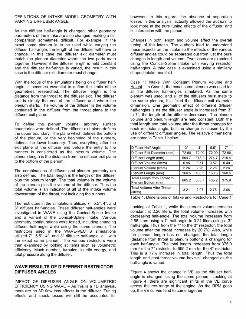
Case 1: Intake With Constant Plenum Volume and Height – In Case 1, the exact same plenum was used for all the diffuser half-angles simulated. As the same plenum was used, and all of the diffusers must mate to the same plenum, this fixed the diffuser exit diameter dimension. One geometric effect of different diffuser half-angles is as the diffuser angle is increased from 3° to 7°, the length of the diffuser decreases. The plenum volume and plenum length are held constant. Both the total length and total volume after the throat changes for each restrictor angle, but the change is caused by the use of different diffuser angles. The relative dimensions are noted in Table 1 below.
Diffuser Half-Angle 3° 4° 5.5° 7°Diffuser Exit Diameter (mm) 72.90 72.90 72.90 72.90Diffuser Length (mm) 504.7 378.2 274.7 215.4Diffuser Volume (liters) 0.95 0.71 0.52 0.40Plenum Volume (liters) 2.26 2.26 2.26 2.26Plenum Length (mm) 160.5 160.5 160.5 160.5Total Length from Throat to Plenum Bottom (mm) 665.2 538.7 435.2 375.9
Total Volume After Throat (liters) 3.21 2.97 2.78 2.66
Table 1. Dimensions of Intake and Restrictors for Case 1
Looking at Table 1, while the plenum volume remains constant at 2.26 liters, the total volume increases with decreasing half-angle. The total volume increases from 2.66 liters using a 7° half-angle to 3.21 liters using a 3° half-angle. Thus from the 7° to the 3° restrictor, the total volume after the throat increases by 20.7%. Also, while the plenum length has not changed, the total length (distance from throat to plenum bottom) is changing for each half-angle. The total length increases from 375.9 mm for the 7° restrictor to 665.2 mm for the 4° restrictor. This is a 77% increase in total length. Thus the total length and post-throat volume have all changed as the half-angle is varied.
Figure 4 shows the change in VE as the diffuser half-angle is changed, using the same plenum. Looking at Figure 4, there are significant shifts in the VE curve across the rev range of the engine. As the RPM goes up, the VE curves tend to come together.
5
The 5.5° restrictor has more volume than the 7°, yet the 5.5° shows a much lower VE from 11,000 to 14,000 RPM. The 4° restrictor also shows a lower VE than the 7° restrictor from 12,250 to 13,000 RPM. This indicates there is more to the determination of a VE curve than plenum volume or the total volume after the throat.
Figure 4. Case 1: Volumetric Efficiency for Various Diffuser Half-Angles with Constant Exit Diameter
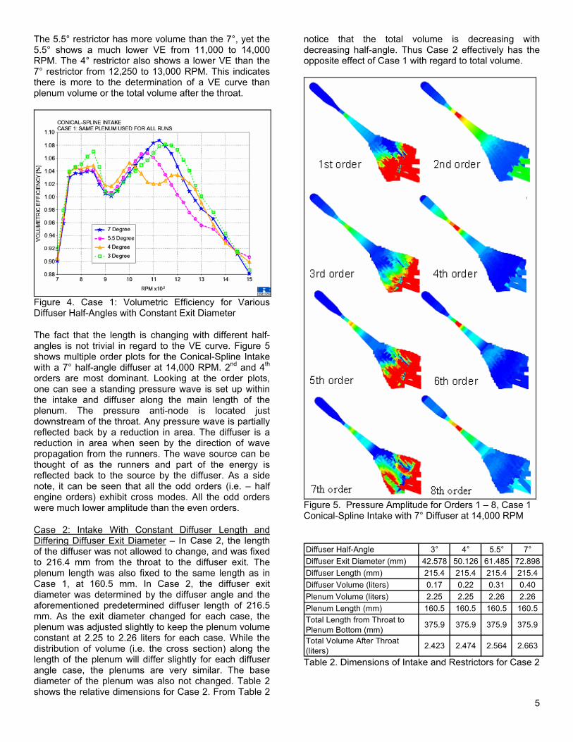
The fact that the length is changing with different half-angles is not trivial in regard to the VE curve. Figure 5 shows multiple order plots for the Conical-Spline Intake with a 7° half-angle diffuser at 14,000 RPM. 2nd and 4th orders are most dominant. Looking at the order plots, one can see a standing pressure wave is set up within the intake and diffuser along the main length of the plenum. The pressure anti-node is located just downstream of the throat. Any pressure wave is partially reflected back by a reduction in area. The diffuser is a reduction in area when seen by the direction of wave propagation from the runners. The wave source can be thought of as the runners and part of the energy is reflected back to the source by the diffuser. As a side note, it can be seen that all the odd orders (i.e. – half engine orders) exhibit cross modes. All the odd orders were much lower amplitude than the even orders.
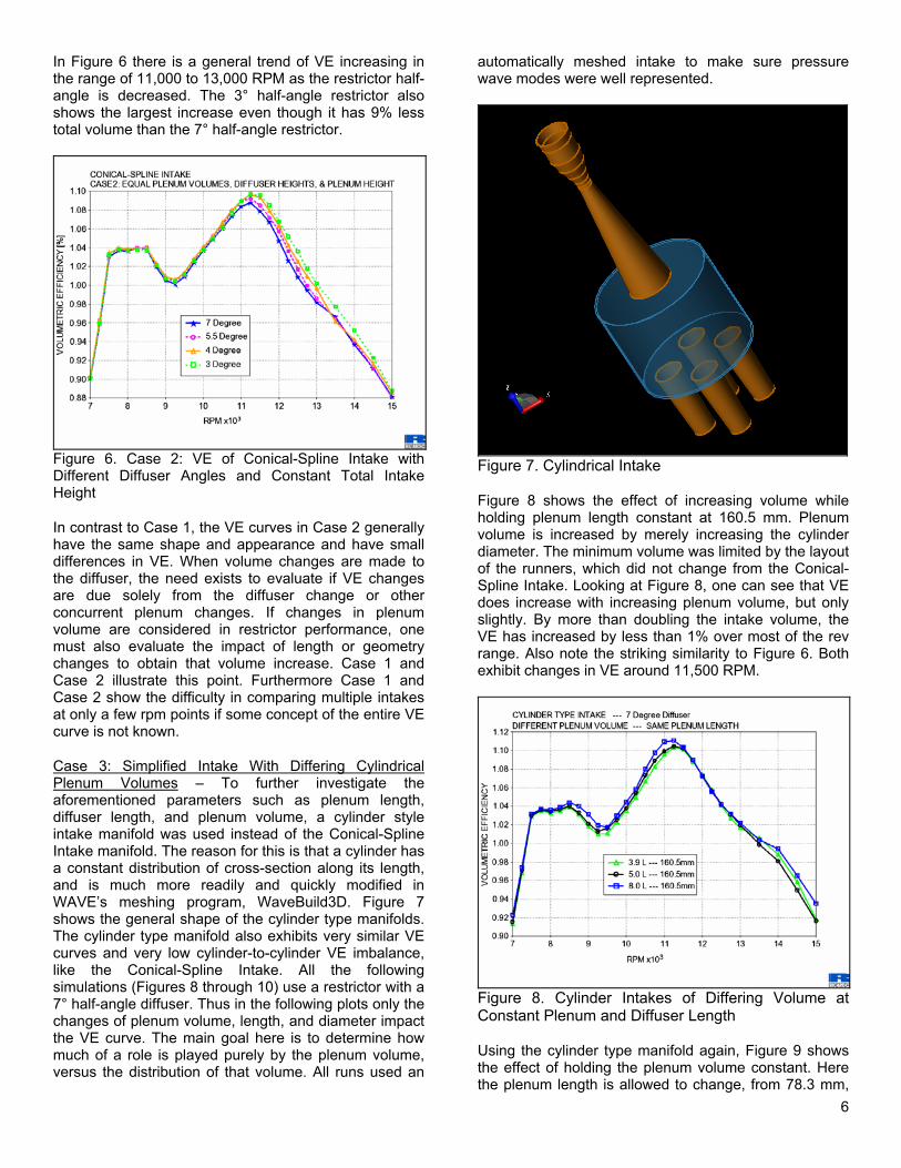
Case 2: Intake With Constant Diffuser Length and Differing Diffuser Exit Diameter – In Case 2, the length of the diffuser was not allowed to change, and was fixed to 216.4 mm from the throat to the diffuser exit. The plenum length was also fixed to the same length as in Case 1, at 160.5 mm. In Case 2, the diffuser exit diameter was determined by the diffuser angle and the aforementioned predetermined diffuser length of 216.5 mm. As the exit diameter changed for each case, the plenum was adjusted slightly to keep the plenum volume constant at 2.25 to 2.26 liters for each case. While the distribution of volume (i.e. the cross section) along the length of the plenum will differ slightly for each diffuser angle case, the plenums are very similar. The base diameter of the plenum was also not changed. Table 2 shows the relative dimensions for Case 2. From Table 2
notice that the total volume is decreasing with decreasing half-angle. Thus Case 2 effectively has the opposite effect of Case 1 with regard to total volume.
Figure 5. Pressure Amplitude for Orders 1 – 8, Case 1 Conical-Spline Intake with 7° Diffuser at 14,000 RPM
Diffuser Half-Angle 3° 4° 5.5° 7°Diffuser Exit Diameter (mm) 42.578 50.126 61.485 72.898Diffuser Length (mm) 215.4 215.4 215.4 215.4Diffuser Volume (liters) 0.17 0.22 0.31 0.40Plenum Volume (liters) 2.25 2.25 2.26 2.26Plenum Length (mm) 160.5 160.5 160.5 160.5Total Length from Throat to Plenum Bottom (mm) 375.9 375.9 375.9 375.9
Total Volume After Throat (liters) 2.423 2.474 2.564 2.663
Table 2. Dimensions of Intake and Restrictors for Case 2
6
In Figure 6 there is a general trend of VE increasing in the range of 11,000 to 13,000 RPM as the restrictor half-angle is decreased. The 3° half-angle restrictor also shows the largest increase even though it has 9% less total volume than the 7° half-angle restrictor.
Figure 6. Case 2: VE of Conical-Spline Intake with Different Diffuser Angles and Constant Total Intake Height
In contrast to Case 1, the VE curves in Case 2 generally have the same shape and appearance and have small differences in VE. When volume changes are made to the diffuser, the need exists to evaluate if VE changes are due solely from the diffuser change or other concurrent plenum changes. If changes in plenum volume are considered in restrictor performance, one must also evaluate the impact of length or geometry changes to obtain that volume increase. Case 1 and Case 2 illustrate this point. Furthermore Case 1 and Case 2 show the difficulty in comparing multiple intakes at only a few rpm points if some concept of the entire VE curve is not known.
Case 3: Simplified Intake With Differing Cylindrical Plenum Volumes – To further investigate the aforementioned parameters such as plenum length, diffuser length, and plenum volume, a cylinder style intake manifold was used instead of the Conical-Spline Intake manifold. The reason for this is that a cylinder has a constant distribution of cross-section along its length, and is much more readily and quickly modified in WAVE’s meshing program, WaveBuild3D. Figure 7 shows the general shape of the cylinder type manifolds. The cylinder type manifold also exhibits very similar VE curves and very low cylinder-to-cylinder VE imbalance, like the Conical-Spline Intake. All the following simulations (Figures 8 through 10) use a restrictor with a 7° half-angle diffuser. Thus in the following plots only the changes of plenum volume, length, and diameter impact the VE curve. The main goal here is to determine how much of a role is played purely by the plenum volume, versus the distribution of that volume. All runs used an
automatically meshed intake to make sure pressure wave modes were well represented.
Figure 7. Cylindrical Intake
Figure 8 shows the effect of increasing volume while holding plenum length constant at 160.5 mm. Plenum volume is increased by merely increasing the cylinder diameter. The minimum volume was limited by the layout of the runners, which did not change from the Conical-Spline Intake. Looking at Figure 8, one can see that VE does increase with increasing plenum volume, but only slightly. By more than doubling the intake volume, the VE has increased by less than 1% over most of the rev range. Also note the striking similarity to Figure 6. Both exhibit changes in VE around 11,500 RPM.
Figure 8. Cylinder Intakes of Differing Volume at Constant Plenum and Diffuser Length
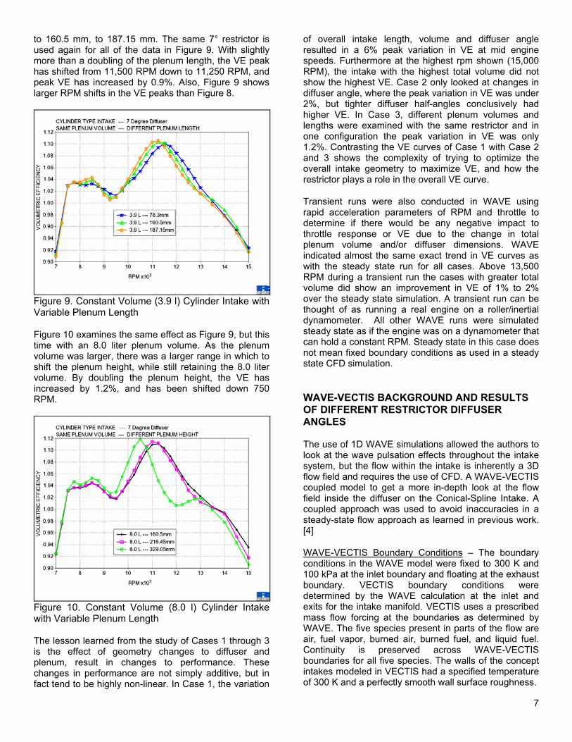
Using the cylinder type manifold again, Figure 9 shows the effect of holding the plenum volume constant. Here the plenum length is allowed to change, from 78.3 mm,
7
to 160.5 mm, to 187.15 mm. The same 7° restrictor is used again for all of the data in Figure 9. With slightly more than a doubling of the plenum length, the VE peak has shifted from 11,500 RPM down to 11,250 RPM, and peak VE has increased by 0.9%. Also, Figure 9 shows larger RPM shifts in the VE peaks than Figure 8.
Figure 9. Constant Volume (3.9 l) Cylinder Intake with Variable Plenum Length
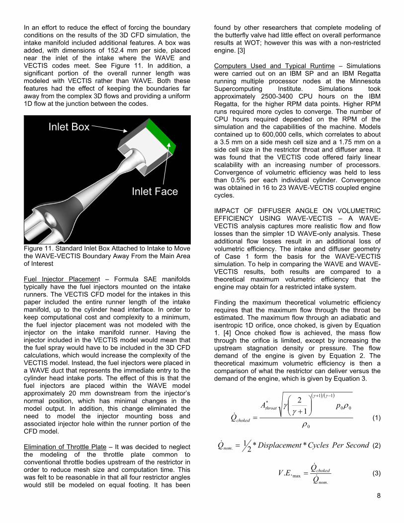
Figure 10 examines the same effect as Figure 9, but this time with an 8.0 liter plenum volume. As the plenum volume was larger, there was a larger range in which to shift the plenum height, while still retaining the 8.0 liter volume. By doubling the plenum height, the VE has increased by 1.2%, and has been shifted down 750 RPM.
Figure 10. Constant Volume (8.0 l) Cylinder Intake with Variable Plenum Length
The lesson learned from the study of Cases 1 through 3 is the effect of geometry changes to diffuser and plenum, result in changes to performance. These changes in performance are not simply additive, but in fact tend to be highly non-linear. In Case 1, the variation
of overall intake length, volume and diffuser angle resulted in a 6% peak variation in VE at mid engine speeds. Furthermore at the highest rpm shown (15,000 RPM), the intake with the highest total volume did not show the highest VE. Case 2 only looked at changes in diffuser angle, where the peak variation in VE was under 2%, but tighter diffuser half-angles conclusively had higher VE. In Case 3, different plenum volumes and lengths were examined with the same restrictor and in one configuration the peak variation in VE was only 1.2%. Contrasting the VE curves of Case 1 with Case 2 and 3 shows the complexity of trying to optimize the overall intake geometry to maximize VE, and how the restrictor plays a role in the overall VE curve.
Transient runs were also conducted in WAVE using rapid acceleration parameters of RPM and throttle to determine if there would be any negative impact to throttle response or VE due to the change in total plenum volume and/or diffuser dimensions. WAVE indicated almost the same exact trend in VE curves as with the steady state run for all cases. Above 13,500 RPM during a transient run the cases with greater total volume did show an improvement in VE of 1% to 2% over the steady state simulation. A transient run can be thought of as running a real engine on a roller/inertial dynamometer. All other WAVE runs were simulated steady state as if the engine was on a dynamometer that can hold a constant RPM. Steady state in this case does not mean fixed boundary conditions as used in a steady state CFD simulation.
WAVE-VECTIS BACKGROUND AND RESULTS OF DIFFERENT RESTRICTOR DIFFUSER ANGLES
The use of 1D WAVE simulations allowed the authors to look at the wave pulsation effects throughout the intake system, but the flow within the intake is inherently a 3D flow field and requires the use of CFD. A WAVE-VECTIS coupled model to get a more in-depth look at the flow field inside the diffuser on the Conical-Spline Intake. A coupled approach was used to avoid inaccuracies in a steady-state flow approach as learned in previous work. [4]
WAVE-VECTIS Boundary Conditions – The boundary conditions in the WAVE model were fixed to 300 K and 100 kPa at the inlet boundary and floating at the exhaust boundary. VECTIS boundary conditions were determined by the WAVE calculation at the inlet and exits for the intake manifold. VECTIS uses a prescribed mass flow forcing at the boundaries as determined by WAVE. The five species present in parts of the flow are air, fuel vapor, burned air, burned fuel, and liquid fuel. Continuity is preserved across WAVE-VECTIS boundaries for all five species. The walls of the concept intakes modeled in VECTIS had a specified temperature of 300 K and a perfectly smooth wall surface roughness.
8
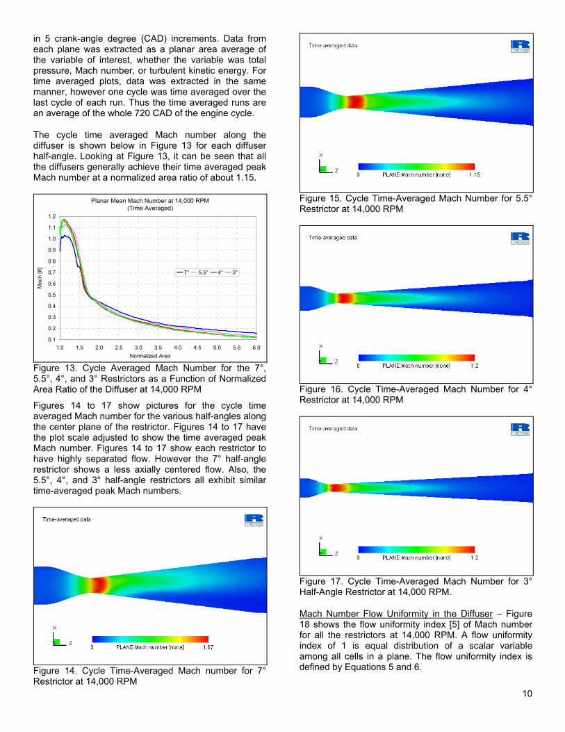
In an effort to reduce the effect of forcing the boundary conditions on the results of the 3D CFD simulation, the intake manifold included additional features. A box was added, with dimensions of 152.4 mm per side, placed near the inlet of the intake where the WAVE and VECTIS codes meet. See Figure 11. In addition, a significant portion of the overall runner length was modeled with VECTIS rather than WAVE. Both these features had the effect of keeping the boundaries far away from the complex 3D flows and providing a uniform 1D flow at the junction between the codes.
Figure 11. Standard Inlet Box Attached to Intake to Move the WAVE-VECTIS Boundary Away From the Main Area of Interest
Fuel Injector Placement – Formula SAE manifolds typically have the fuel injectors mounted on the intake runners. The VECTIS CFD model for the intakes in this paper included the entire runner length of the intake manifold, up to the cylinder head interface. In order to keep computational cost and complexity to a minimum, the fuel injector placement was not modeled with the injector on the intake manifold runner. Having the injector included in the VECTIS model would mean that the fuel spray would have to be included in the 3D CFD calculations, which would increase the complexity of the VECTIS model. Instead, the fuel injectors were placed in a WAVE duct that represents the immediate entry to the cylinder head intake ports. The effect of this is that the fuel injectors are placed within the WAVE model approximately 20 mm downstream from the injector’s normal position, which has minimal changes in the model output. In addition, this change eliminated the need to model the injector mounting boss and associated injector hole within the runner portion of the CFD model.
Elimination of Throttle Plate – It was decided to neglect the modeling of the throttle plate common to conventional throttle bodies upstream of the restrictor in order to reduce mesh size and computation time. This was felt to be reasonable in that all four restrictor angles would still be modeled on equal footing. It has been
found by other researchers that complete modeling of the butterfly valve had little effect on overall performance results at WOT; however this was with a non-restricted engine. [3]
Computers Used and Typical Runtime – Simulations were carried out on an IBM SP and an IBM Regatta running multiple processor nodes at the Minnesota Supercomputing Institute. Simulations took approximately 2500-3400 CPU hours on the IBM Regatta, for the higher RPM data points. Higher RPM runs required more cycles to converge. The number of CPU hours required depended on the RPM of the simulation and the capabilities of the machine. Models contained up to 600,000 cells, which correlates to about a 3.5 mm on a side mesh cell size and a 1.75 mm on a side cell size in the restrictor throat and diffuser area. It was found that the VECTIS code offered fairly linear scalability with an increasing number of processors. Convergence of volumetric efficiency was held to less than 0.5% per each individual cylinder. Convergence was obtained in 16 to 23 WAVE-VECTIS coupled engine cycles.
IMPACT OF DIFFUSER ANGLE ON VOLUMETRIC EFFICIENCY USING WAVE-VECTIS – A WAVE-VECTIS analysis captures more realistic flow and flow losses than the simpler 1D WAVE-only analysis. These additional flow losses result in an additional loss of volumetric efficiency. The intake and diffuser geometry of Case 1 form the basis for the WAVE-VECTIS simulation. To help in comparing the WAVE and WAVE-VECTIS results, both results are compared to a theoretical maximum volumetric efficiency that the engine may obtain for a restricted intake system.
Finding the maximum theoretical volumetric efficiency requires that the maximum flow through the throat be estimated. The maximum flow through an adiabatic and isentropic 1D orifice, once choked, is given by Equation 1. [4] Once choked flow is achieved, the mass flow through the orifice is limited, except by increasing the upstream stagnation density or pressure. The flow demand of the engine is given by Equation 2. The theoretical maximum volumetric efficiency is then a comparison of what the restrictor can deliver versus the demand of the engine, which is given by Equation 3.
( ) ( )
0
00
11*
12
ρ
ργ
γγγ
pAQ
throat
choked
−+
+
=& (1)
SecondPerCyclesntDisplacemeQnom **21
. =& (2)
.max..
nom
choked
QQEV&
&= (3)
Inlet Box
Inlet Face

9
The theoretical maximum volumetric efficiency is compared to the WAVE and WAVE-VECTIS results in Figure 12. Some data points closely overlap each other in Figure 12, thus Table 3 shows the actual volumetric efficiencies.
0.85
0.90
0.95
1.00
1.05
1.10
1.15
1.20
1.25
9000 10000 11000 12000 13000 14000 15000RPM
VO
LUM
ETR
IC E
FFIC
IEN
CY
Theoretical Maximum7 Degree - WAVE 7 Degree - WAVE-VECTIS 5.5 Degree - WAVE 5.5 Degree - WAVE-VECTIS 4 Degree - WAVE 4 Degree - WAVE-VECTIS 3 Degree - WAVE 3 Degree - WAVE-VECTIS
Figure 12. Theoretical Maximum Volumetric Efficiency Compared to the WAVE and WAVE-VECTIS Simulations Beyond approximately 12,000 RPM, the WAVE simulations display a VE that is above the theoretical maximum VE. However, some of the WAVE-VECTIS data points also exceed the theoretical maximum VE, as shown in Figure 12 and Table 3. If the diffuser and intake system are designed well, then the system should approach the maximum theoretical volumetric efficiency at high RPM. Looking at Table 3, the 5.5° half-angle diffuser comes within 0.1% of matching the theoretical maximum VE, whereas the 4° half-angle diffuser exceeds the theoretical maximum VE by 0.9%. The 3° half-angle diffuser exceeds the theoretical maximum VE by 1.3%.
Theoretical Maximum
Wave-Vectis Wave Difference
(Wave - W-V)7° 10 126.5% 97.2% 103.7% 6.5%4° 10 126.5% 101.3% 105.3% 4.0%7° 11.5 110.0% 100.5% 107.9% 7.4%7° 14 90.4% 87.8% 93.7% 5.9%
5.5° 14 90.4% 90.3% 93.2% 2.9%4° 14 90.4% 91.3% 92.9% 1.6%3° 14 90.4% 91.7% 94.3% 2.6%
Half Angle
RPM x1000
VOLUMETRIC EFFICIENCY
Table 3. Comparison of WAVE and WAVE-VECTIS Simulations to Theoretical Maximum Volumetric Efficiency
While the maximum theoretical VE gives a good indicator of the performance achievable for a particular engine, especially as RPM increases, it is not the final word on the maximum VE achievable. Equation 3 makes an implicit assumption wherein the unsteady, cycle dependent flow through the valves is deemed to be
equal to the steady state flow through the restrictor. The flow through the valves is highly unsteady, with pulse tuning of the runners and intake plenum also occurring. The pressure during intake valve closure, due to cam timing and pressure wave tuning is of prime importance in dictating VE. Thus looking purely at the steady flow through the throat is too simplistic to analyze the maximum obtainable VE.
The implicit assumption is made by Equations 1 and 3 that the flow is choked 100% of the time, which does not occur in engine operation even at 14,000 RPM according to simulation results. The 7° half-angle restrictor at 10,000 RPM does not achieve choked flow (as will be shown later), yet there is still a large disparity in volumetric efficiency between the WAVE and WAVE-VECTIS solution. However both the WAVE and WAVE-VECTIS solutions for the 7° half-angle restrictor at 10,000 RPM are still well below the theoretical maximum VE. Thus at 10,000 RPM there are more gains to be obtained, likely through flow loss reductions and tuning, even though the restrictor does not reach Mach 1 during the cycle.
The WAVE-VECTIS simulations all display a VE lower than WAVE. The result that WAVE predicts a higher VE in relation to WAVE-VECTIS is expected, as WAVE simply can not predict 3D flow losses. Looking at Table 3, the very right hand column shows the difference in VE between WAVE and WAVE-VECTIS. The VE difference helps to judge how close each restrictor is to realizing its individual VE potential at each RPM point. Comparing the various restrictors at 14,000 RPM, it can be noted that the 7° restrictor has more VE difference than any of the other restrictors. At 10,000 RPM the VE difference for the 7° restrictor is also greater than the 4° restrictor. This at least implies 3D flow losses are decreasing as restrictor half-angle is decreasing.
The following three sections go into more detail regarding Mach number, turbulent kinetic energy, and total pressure, in the diffuser section.
MACH NUMBER IN THE DIFFUSER – The WAVE-VECTIS results in this section and the following two sections are plotted as a function of a normalized area
ratio. The area ratio is given by Equation 4 where xA is the cross sectional area of the diffuser at some distance
downstream of the throat and *A is the area at the
throat. For reference, the restrictor throat has a normalized are ratio of 1, and the restrictor exit has a normalized area ratio of 13.29.
*AAAreaNormalized x= (4)
To plot the data from the VECTIS portion of the simulation, multiple planes were set up perpendicular to the restrictor flow axis. Data was extracted at each plane
10
in 5 crank-angle degree (CAD) increments. Data from each plane was extracted as a planar area average of the variable of interest, whether the variable was total pressure, Mach number, or turbulent kinetic energy. For time averaged plots, data was extracted in the same manner, however one cycle was time averaged over the last cycle of each run. Thus the time averaged runs are an average of the whole 720 CAD of the engine cycle.
The cycle time averaged Mach number along the diffuser is shown below in Figure 13 for each diffuser half-angle. Looking at Figure 13, it can be seen that all the diffusers generally achieve their time averaged peak Mach number at a normalized area ratio of about 1.15.
Planar Mean Mach Number at 14,000 RPM(Time Averaged)
0.1
0.2
0.3
0.4
0.5
0.6
0.7
0.8
0.9
1.0
1.1
1.2
1.0 1.5 2.0 2.5 3.0 3.5 4.0 4.5 5.0 5.5 6.0Normalized Area
Mac
h [#
]
7° 5.5° 4° 3°
Figure 13. Cycle Averaged Mach Number for the 7°, 5.5°, 4°, and 3° Restrictors as a Function of Normalized Area Ratio of the Diffuser at 14,000 RPM
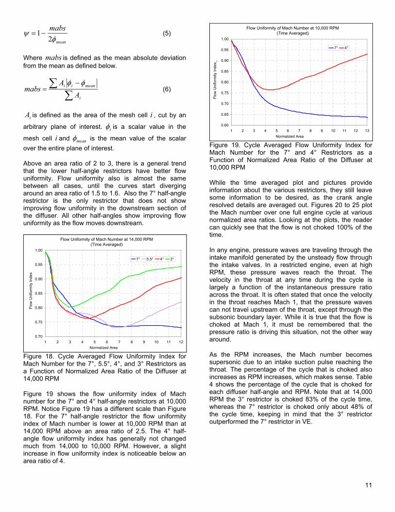
Figures 14 to 17 show pictures for the cycle time averaged Mach number for the various half-angles along the center plane of the restrictor. Figures 14 to 17 have the plot scale adjusted to show the time averaged peak Mach number. Figures 14 to 17 show each restrictor to have highly separated flow. However the 7° half-angle restrictor shows a less axially centered flow. Also, the 5.5°, 4°, and 3° half-angle restrictors all exhibit similar time-averaged peak Mach numbers.
Figure 14. Cycle Time-Averaged Mach number for 7° Restrictor at 14,000 RPM
Figure 15. Cycle Time-Averaged Mach Number for 5.5° Restrictor at 14,000 RPM
Figure 16. Cycle Time-Averaged Mach Number for 4° Restrictor at 14,000 RPM
Figure 17. Cycle Time-Averaged Mach Number for 3° Half-Angle Restrictor at 14,000 RPM.
Mach Number Flow Uniformity in the Diffuser – Figure 18 shows the flow uniformity index [5] of Mach number for all the restrictors at 14,000 RPM. A flow uniformity index of 1 is equal distribution of a scalar variable among all cells in a plane. The flow uniformity index is defined by Equations 5 and 6.
11
mean
mabsφ
ψ2
1−= (5)
Where mabs is defined as the mean absolute deviation from the mean as defined below.
∑∑ −
=i
meanii
AA
mabsφφ
(6)
iA is defined as the area of the mesh cell i , cut by an
arbitrary plane of interest. iφ is a scalar value in the
mesh cell i and meanφ is the mean value of the scalar over the entire plane of interest.
Above an area ratio of 2 to 3, there is a general trend that the lower half-angle restrictors have better flow uniformity. Flow uniformity also is almost the same between all cases, until the curves start diverging around an area ratio of 1.5 to 1.6. Also the 7° half-angle restrictor is the only restrictor that does not show improving flow uniformity in the downstream section of the diffuser. All other half-angles show improving flow uniformity as the flow moves downstream.
Flow Uniformity of Mach Number at 14,000 RPM(Time Averaged)
0.70
0.75
0.80
0.85
0.90
0.95
1.00
1 2 3 4 5 6 7 8 9 10 11 12Normalized Area
Flow
Uni
form
ity In
dex
7° 5.5° 4° 3°
Figure 18. Cycle Averaged Flow Uniformity Index for Mach Number for the 7°, 5.5°, 4°, and 3° Restrictors as a Function of Normalized Area Ratio of the Diffuser at 14,000 RPM
Figure 19 shows the flow uniformity index of Mach number for the 7° and 4° half-angle restrictors at 10,000 RPM. Notice Figure 19 has a different scale than Figure 18. For the 7° half-angle restrictor the flow uniformity index of Mach number is lower at 10,000 RPM than at 14,000 RPM above an area ratio of 2.5. The 4° half-angle flow uniformity index has generally not changed much from 14,000 to 10,000 RPM. However, a slight increase in flow uniformity index is noticeable below an area ratio of 4.
Flow Uniformity of Mach Number at 10,000 RPM(Time Averaged)
0.60
0.65
0.70
0.75
0.80
0.85
0.90
0.95
1.00
1 2 3 4 5 6 7 8 9 10 11 12 13Normalized Area
Flow
Uni
form
ity In
dex_
7° 4°
Figure 19. Cycle Averaged Flow Uniformity Index for Mach Number for the 7° and 4° Restrictors as a Function of Normalized Area Ratio of the Diffuser at 10,000 RPM
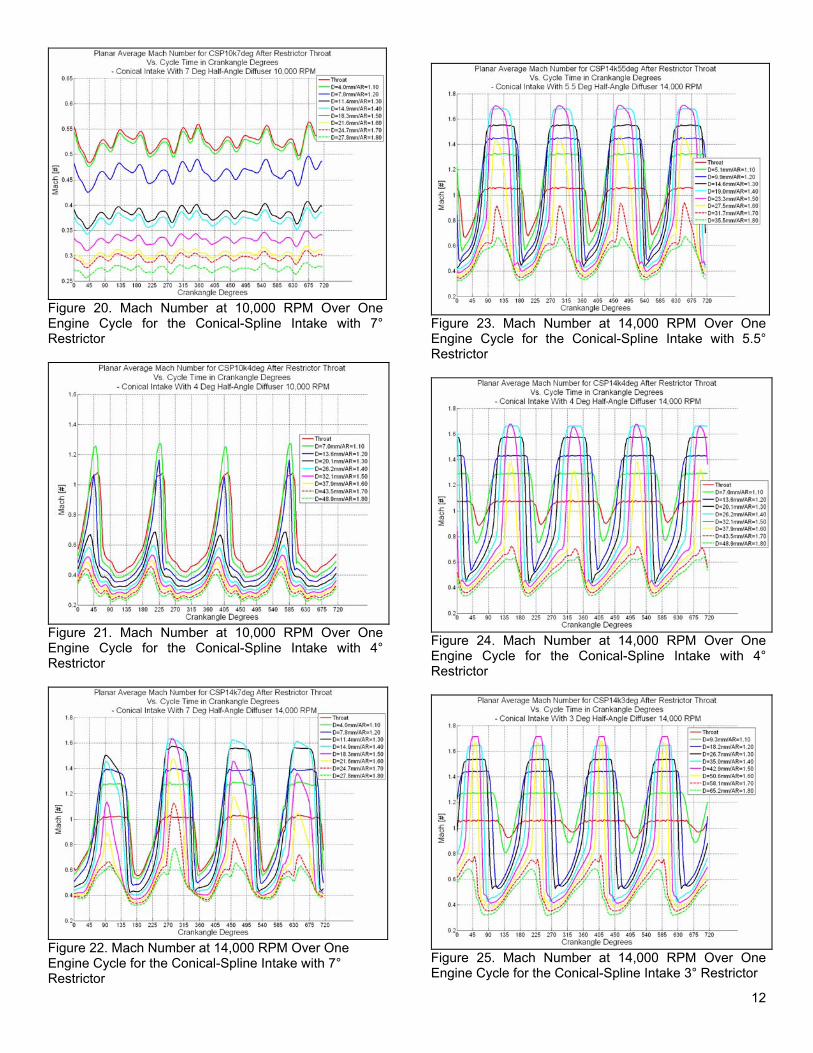
While the time averaged plot and pictures provide information about the various restrictors, they still leave some information to be desired, as the crank angle resolved details are averaged out. Figures 20 to 25 plot the Mach number over one full engine cycle at various normalized area ratios. Looking at the plots, the reader can quickly see that the flow is not choked 100% of the time.
In any engine, pressure waves are traveling through the intake manifold generated by the unsteady flow through the intake valves. In a restricted engine, even at high RPM, these pressure waves reach the throat. The velocity in the throat at any time during the cycle is largely a function of the instantaneous pressure ratio across the throat. It is often stated that once the velocity in the throat reaches Mach 1, that the pressure waves can not travel upstream of the throat, except through the subsonic boundary layer. While it is true that the flow is choked at Mach 1, it must be remembered that the pressure ratio is driving this situation, not the other way around.
As the RPM increases, the Mach number becomes supersonic due to an intake suction pulse reaching the throat. The percentage of the cycle that is choked also increases as RPM increases, which makes sense. Table 4 shows the percentage of the cycle that is choked for each diffuser half-angle and RPM. Note that at 14,000 RPM the 3° restrictor is choked 83% of the cycle time, whereas the 7° restrictor is choked only about 48% of the cycle time, keeping in mind that the 3° restrictor outperformed the 7° restrictor in VE.
12
Figure 20. Mach Number at 10,000 RPM Over One Engine Cycle for the Conical-Spline Intake with 7° Restrictor
Figure 21. Mach Number at 10,000 RPM Over One Engine Cycle for the Conical-Spline Intake with 4° Restrictor
Figure 22. Mach Number at 14,000 RPM Over One Engine Cycle for the Conical-Spline Intake with 7° Restrictor
Figure 23. Mach Number at 14,000 RPM Over One Engine Cycle for the Conical-Spline Intake with 5.5° Restrictor
Figure 24. Mach Number at 14,000 RPM Over One Engine Cycle for the Conical-Spline Intake with 4° Restrictor
Figure 25. Mach Number at 14,000 RPM Over One Engine Cycle for the Conical-Spline Intake 3° Restrictor
13
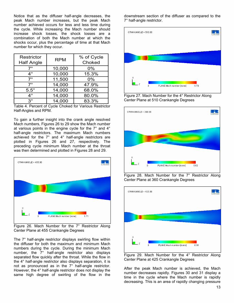
Notice that as the diffuser half-angle decreases, the peak Mach number increases, but the peak Mach number achieved occurs for less and less time during the cycle. While increasing the Mach number should increase shock losses, the shock losses are a combination of both the Mach number at which the shocks occur, plus the percentage of time at that Mach number for which they occur.
Restrictor Half Angle RPM % of Cycle
Choked7° 10,000 0%4° 10,000 15.3%7° 11,500 0%7° 14,000 47.9%
5.5° 14,000 68.0%4° 14,000 80.0%3° 14,000 83.3%
Table 4. Percent of Cycle Choked for Various Restrictor Half-Angles and RPM.
To gain a further insight into the crank angle resolved Mach numbers, Figures 26 to 29 show the Mach number at various points in the engine cycle for the 7° and 4° half-angle restrictors. The maximum Mach numbers achieved for the 7° and 4° half-angle restrictors are plotted in Figures 26 and 27, respectively. The preceding cycle minimum Mach number at the throat was then determined and plotted in Figures 28 and 29.
Figure 26. Mach Number for the 7° Restrictor Along Center Plane at 455 Crankangle Degrees
The 7° half-angle restrictor displays swirling flow within the diffuser for both the maximum and minimum Mach numbers during the cycle. During the minimum Mach number, the 7° half-angle restrictor also displays separated flow quickly after the throat. While the flow in the 4° half-angle restrictor also displays separation, it is not as pronounced as in the 7° half-angle restrictor. However, the 4° half-angle restrictor does not display the same high degree of swirling of the flow in the
downstream section of the diffuser as compared to the 7° half-angle restrictor.
Figure 27. Mach Number for the 4° Restrictor Along Center Plane at 510 Crankangle Degrees
Figure 28. Mach Number for the 7° Restrictor Along Center Plane at 360 Crankangle Degrees
Figure 29. Mach Number for the 4° Restrictor Along Center Plane at 425 Crankangle Degrees
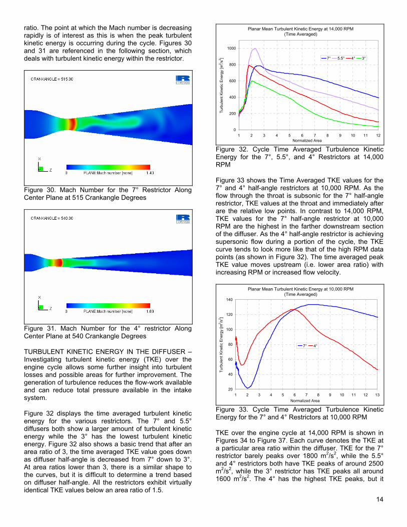
After the peak Mach number is achieved, the Mach number decreases rapidly. Figures 30 and 31 display a time in the cycle where the Mach number is rapidly decreasing. This is an area of rapidly changing pressure
14
ratio. The point at which the Mach number is decreasing rapidly is of interest as this is when the peak turbulent kinetic energy is occurring during the cycle. Figures 30 and 31 are referenced in the following section, which deals with turbulent kinetic energy within the restrictor.
Figure 30. Mach Number for the 7° Restrictor Along Center Plane at 515 Crankangle Degrees
Figure 31. Mach Number for the 4° restrictor Along Center Plane at 540 Crankangle Degrees
TURBULENT KINETIC ENERGY IN THE DIFFUSER –Investigating turbulent kinetic energy (TKE) over the engine cycle allows some further insight into turbulent losses and possible areas for further improvement. The generation of turbulence reduces the flow-work available and can reduce total pressure available in the intake system.
Figure 32 displays the time averaged turbulent kinetic energy for the various restrictors. The 7° and 5.5° diffusers both show a larger amount of turbulent kinetic energy while the 3° has the lowest turbulent kinetic energy. Figure 32 also shows a basic trend that after an area ratio of 3, the time averaged TKE value goes down as diffuser half-angle is decreased from 7° down to 3°. At area ratios lower than 3, there is a similar shape to the curves, but it is difficult to determine a trend based on diffuser half-angle. All the restrictors exhibit virtually identical TKE values below an area ratio of 1.5.
Planar Mean Turbulent Kinetic Energy at 14,000 RPM(Time Averaged)
0
200
400
600
800
1000
1 2 3 4 5 6 7 8 9 10 11 12Normalized Area
Turb
ulen
t Kin
etic
Ene
rgy
[m2 /s
2 ] 7° 5.5° 4° 3°
Figure 32. Cycle Time Averaged Turbulence Kinetic Energy for the 7°, 5.5°, and 4° Restrictors at 14,000 RPM
Figure 33 shows the Time Averaged TKE values for the 7° and 4° half-angle restrictors at 10,000 RPM. As the flow through the throat is subsonic for the 7° half-angle restrictor, TKE values at the throat and immediately after are the relative low points. In contrast to 14,000 RPM, TKE values for the 7° half-angle restrictor at 10,000 RPM are the highest in the farther downstream section of the diffuser. As the 4° half-angle restrictor is achieving supersonic flow during a portion of the cycle, the TKE curve tends to look more like that of the high RPM data points (as shown in Figure 32). The time averaged peak TKE value moves upstream (i.e. lower area ratio) with increasing RPM or increased flow velocity.
Planar Mean Turbulent Kinetic Energy at 10,000 RPM(Time Averaged)
20
40
60
80
100
120
140
1 2 3 4 5 6 7 8 9 10 11 12 13Normalized Area
Turb
ulen
t Kin
etic
Ene
rgy
[m2 /s
2 ]
7° 4°
Figure 33. Cycle Time Averaged Turbulence Kinetic Energy for the 7° and 4° Restrictors at 10,000 RPM
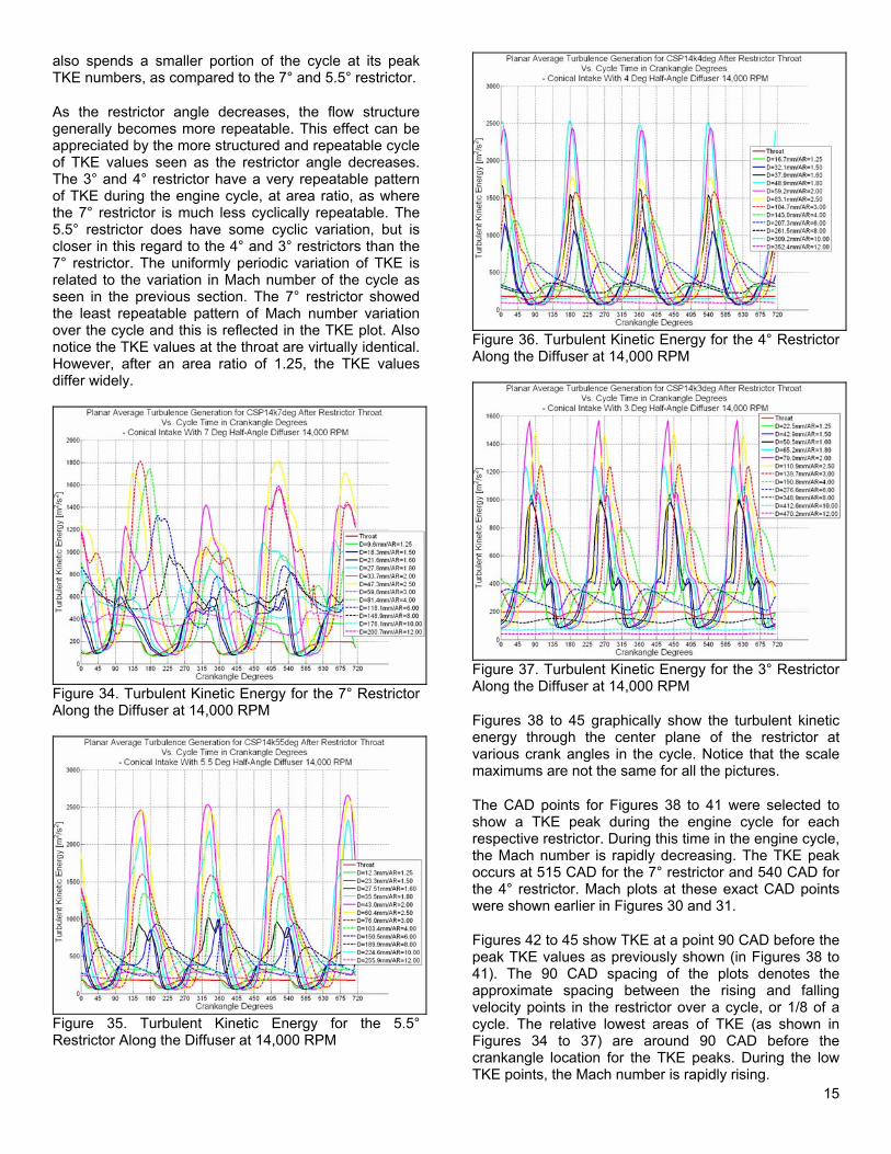
TKE over the engine cycle at 14,000 RPM is shown in Figures 34 to Figure 37. Each curve denotes the TKE at a particular area ratio within the diffuser. TKE for the 7° restrictor barely peaks over 1800 m2/s2, while the 5.5° and 4° restrictors both have TKE peaks of around 2500 m2/s2, while the 3° restrictor has TKE peaks all around 1600 m2/s2. The 4° has the highest TKE peaks, but it
15
also spends a smaller portion of the cycle at its peak TKE numbers, as compared to the 7° and 5.5° restrictor.
As the restrictor angle decreases, the flow structure generally becomes more repeatable. This effect can be appreciated by the more structured and repeatable cycle of TKE values seen as the restrictor angle decreases. The 3° and 4° restrictor have a very repeatable pattern of TKE during the engine cycle, at area ratio, as where the 7° restrictor is much less cyclically repeatable. The 5.5° restrictor does have some cyclic variation, but is closer in this regard to the 4° and 3° restrictors than the 7° restrictor. The uniformly periodic variation of TKE is related to the variation in Mach number of the cycle as seen in the previous section. The 7° restrictor showed the least repeatable pattern of Mach number variation over the cycle and this is reflected in the TKE plot. Also notice the TKE values at the throat are virtually identical. However, after an area ratio of 1.25, the TKE values differ widely.
Figure 34. Turbulent Kinetic Energy for the 7° Restrictor Along the Diffuser at 14,000 RPM
Figure 35. Turbulent Kinetic Energy for the 5.5° Restrictor Along the Diffuser at 14,000 RPM
Figure 36. Turbulent Kinetic Energy for the 4° Restrictor Along the Diffuser at 14,000 RPM
Figure 37. Turbulent Kinetic Energy for the 3° Restrictor Along the Diffuser at 14,000 RPM
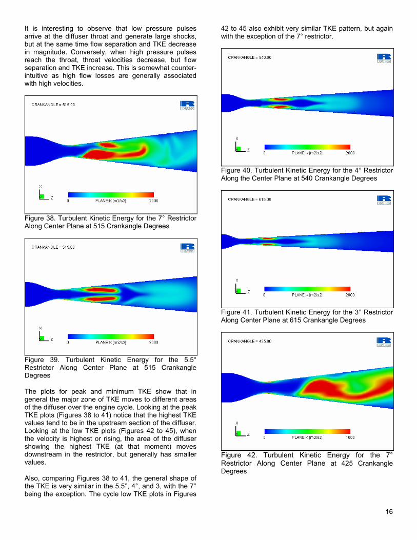
Figures 38 to 45 graphically show the turbulent kinetic energy through the center plane of the restrictor at various crank angles in the cycle. Notice that the scale maximums are not the same for all the pictures.
The CAD points for Figures 38 to 41 were selected to show a TKE peak during the engine cycle for each respective restrictor. During this time in the engine cycle, the Mach number is rapidly decreasing. The TKE peak occurs at 515 CAD for the 7° restrictor and 540 CAD for the 4° restrictor. Mach plots at these exact CAD points were shown earlier in Figures 30 and 31.
Figures 42 to 45 show TKE at a point 90 CAD before the peak TKE values as previously shown (in Figures 38 to 41). The 90 CAD spacing of the plots denotes the approximate spacing between the rising and falling velocity points in the restrictor over a cycle, or 1/8 of a cycle. The relative lowest areas of TKE (as shown in Figures 34 to 37) are around 90 CAD before the crankangle location for the TKE peaks. During the low TKE points, the Mach number is rapidly rising.
16
It is interesting to observe that low pressure pulses arrive at the diffuser throat and generate large shocks, but at the same time flow separation and TKE decrease in magnitude. Conversely, when high pressure pulses reach the throat, throat velocities decrease, but flow separation and TKE increase. This is somewhat counter-intuitive as high flow losses are generally associated with high velocities.
Figure 38. Turbulent Kinetic Energy for the 7° Restrictor Along Center Plane at 515 Crankangle Degrees
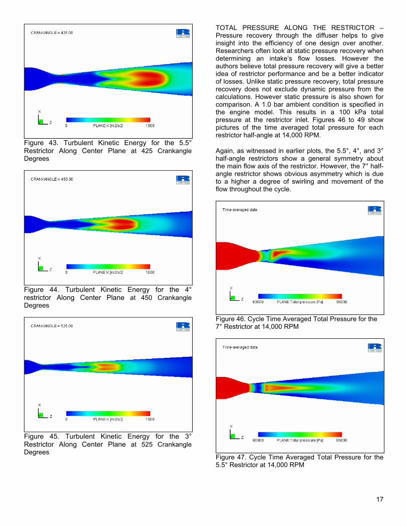
Figure 39. Turbulent Kinetic Energy for the 5.5° Restrictor Along Center Plane at 515 Crankangle Degrees
The plots for peak and minimum TKE show that in general the major zone of TKE moves to different areas of the diffuser over the engine cycle. Looking at the peak TKE plots (Figures 38 to 41) notice that the highest TKE values tend to be in the upstream section of the diffuser. Looking at the low TKE plots (Figures 42 to 45), when the velocity is highest or rising, the area of the diffuser showing the highest TKE (at that moment) moves downstream in the restrictor, but generally has smaller values.
Also, comparing Figures 38 to 41, the general shape of the TKE is very similar in the 5.5°, 4°, and 3, with the 7° being the exception. The cycle low TKE plots in Figures
42 to 45 also exhibit very similar TKE pattern, but again with the exception of the 7° restrictor.
Figure 40. Turbulent Kinetic Energy for the 4° Restrictor Along the Center Plane at 540 Crankangle Degrees
Figure 41. Turbulent Kinetic Energy for the 3° Restrictor Along Center Plane at 615 Crankangle Degrees
Figure 42. Turbulent Kinetic Energy for the 7° Restrictor Along Center Plane at 425 Crankangle Degrees
17
Figure 43. Turbulent Kinetic Energy for the 5.5° Restrictor Along Center Plane at 425 Crankangle Degrees
Figure 44. Turbulent Kinetic Energy for the 4° restrictor Along Center Plane at 450 Crankangle Degrees
Figure 45. Turbulent Kinetic Energy for the 3° Restrictor Along Center Plane at 525 Crankangle Degrees
TOTAL PRESSURE ALONG THE RESTRICTOR –Pressure recovery through the diffuser helps to give insight into the efficiency of one design over another. Researchers often look at static pressure recovery when determining an intake’s flow losses. However the authors believe total pressure recovery will give a better idea of restrictor performance and be a better indicator of losses. Unlike static pressure recovery, total pressure recovery does not exclude dynamic pressure from the calculations. However static pressure is also shown for comparison. A 1.0 bar ambient condition is specified in the engine model. This results in a 100 kPa total pressure at the restrictor inlet. Figures 46 to 49 show pictures of the time averaged total pressure for each restrictor half-angle at 14,000 RPM.
Again, as witnessed in earlier plots, the 5.5°, 4°, and 3° half-angle restrictors show a general symmetry about the main flow axis of the restrictor. However, the 7° half-angle restrictor shows obvious asymmetry which is due to a higher a degree of swirling and movement of the flow throughout the cycle.
Figure 46. Cycle Time Averaged Total Pressure for the 7° Restrictor at 14,000 RPM
Figure 47. Cycle Time Averaged Total Pressure for the 5.5° Restrictor at 14,000 RPM
18
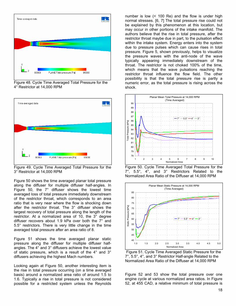
Figure 48. Cycle Time Averaged Total Pressure for the 4° Restrictor at 14,000 RPM
Figure 49. Cycle Time Averaged Total Pressure for the 3° Restrictor at 14,000 RPM
Figure 50 shows the time averaged planar total pressure along the diffuser for multiple diffuser half-angles. In Figure 50, the 7° diffuser shows the lowest time averaged loss of total pressure immediately downstream of the restrictor throat, which corresponds to an area ratio that is very near where the flow is shocking down after the restrictor throat. The 3° diffuser shows the largest recovery of total pressure along the length of the restrictor. At a normalized area of 10, the 3° degree diffuser recovers about 1.9 kPa over both the 7° and 5.5° restrictors. There is very little change in the time averaged total pressure after an area ratio of 8.
Figure 51 shows the time averaged planar static pressure along the diffuser for multiple diffuser half-angles. The 4° and 3° diffusers achieve the lowest value of static pressure, which is a result of the 4° and 3° diffusers achieving the highest Mach numbers.
Looking again at Figure 50, another interesting item is the rise in total pressure occurring (on a time averaged basis) around a normalized area ratio of around 1.5 to 1.6. Typically a rise in total pressure is not considered possible for a restricted system unless the Reynolds
number is low (< 100 Re) and the flow is under high normal stresses. [6, 7] The total pressure rise could not be explained by this phenomenon at this location, but may occur in other portions of the intake manifold. The authors believe that the rise in total pressure, after the restrictor throat maybe due in part, to the pulsation effect within the intake system. Energy enters into the system due to pressure pulses which can cause rises in total pressure. Figure 5, shown previously, helps to visualize the pressure waves with the anti-node of the wave typically appearing immediately downstream of the throat. The restrictor is not choked 100% of the time, which means that the wave pulsations reaching the restrictor throat influence the flow field. The other possibility is that the total pressure rise is partly a numeric error, as the total pressure is rising across the shock.
Planar Mean Total Pressure at 14,000 RPM(Time Averaged)
78
79
80
81
82
83
84
85
86
87
88
89
90
1 2 3 4 5 6 7 8 9 10Normalized Area
Tota
l Pre
ssur
e [k
Pa] 7° 5.5° 4° 3°
Figure 50. Cycle Time Averaged Total Pressure for the 7°, 5.5°, 4°, and 3° Restrictors Related to the Normalized Area Ratio of the Diffuser at 14,000 RPM
Planar Mean Static Pressure at 14,000 RPM(Time Averaged)
40
45
50
55
60
65
70
75
80
85
1.0 1.5 2.0 2.5 3.0 3.5 4.0 4.5 5.0Normalized Area
Sta
tic P
ress
ure
[kP
a]
7° 5.5° 4° 3°
Figure 51. Cycle Time Averaged Static Pressure for the 7°, 5.5°, 4°, and 3° Restrictor Half-angle Related to the Normalized Area Ratio of the Diffuser at 14,000 RPM
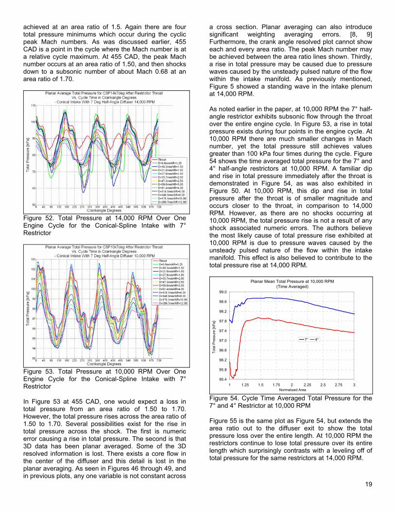
Figure 52 and 53 show the total pressure over one engine cycle at various normalized area ratios. In Figure 52, at 455 CAD, a relative minimum of total pressure is
19
achieved at an area ratio of 1.5. Again there are four total pressure minimums which occur during the cyclic peak Mach numbers. As was discussed earlier, 455 CAD is a point in the cycle where the Mach number is at a relative cycle maximum. At 455 CAD, the peak Mach number occurs at an area ratio of 1.50, and then shocks down to a subsonic number of about Mach 0.68 at an area ratio of 1.70.
Figure 52. Total Pressure at 14,000 RPM Over One Engine Cycle for the Conical-Spline Intake with 7° Restrictor
Figure 53. Total Pressure at 10,000 RPM Over One Engine Cycle for the Conical-Spline Intake with 7° Restrictor
In Figure 53 at 455 CAD, one would expect a loss in total pressure from an area ratio of 1.50 to 1.70. However, the total pressure rises across the area ratio of 1.50 to 1.70. Several possibilities exist for the rise in total pressure across the shock. The first is numeric error causing a rise in total pressure. The second is that 3D data has been planar averaged. Some of the 3D resolved information is lost. There exists a core flow in the center of the diffuser and this detail is lost in the planar averaging. As seen in Figures 46 through 49, and in previous plots, any one variable is not constant across
a cross section. Planar averaging can also introduce significant weighting averaging errors. [8, 9] Furthermore, the crank angle resolved plot cannot show each and every area ratio. The peak Mach number may be achieved between the area ratio lines shown. Thirdly, a rise in total pressure may be caused due to pressure waves caused by the unsteady pulsed nature of the flow within the intake manifold. As previously mentioned, Figure 5 showed a standing wave in the intake plenum at 14,000 RPM.
As noted earlier in the paper, at 10,000 RPM the 7° half-angle restrictor exhibits subsonic flow through the throat over the entire engine cycle. In Figure 53, a rise in total pressure exists during four points in the engine cycle. At 10,000 RPM there are much smaller changes in Mach number, yet the total pressure still achieves values greater than 100 kPa four times during the cycle. Figure 54 shows the time averaged total pressure for the 7° and 4° half-angle restrictors at 10,000 RPM. A familiar dip and rise in total pressure immediately after the throat is demonstrated in Figure 54, as was also exhibited in Figure 50. At 10,000 RPM, this dip and rise in total pressure after the throat is of smaller magnitude and occurs closer to the throat, in comparison to 14,000 RPM. However, as there are no shocks occurring at 10,000 RPM, the total pressure rise is not a result of any shock associated numeric errors. The authors believe the most likely cause of total pressure rise exhibited at 10,000 RPM is due to pressure waves caused by the unsteady pulsed nature of the flow within the intake manifold. This effect is also believed to contribute to the total pressure rise at 14,000 RPM.
Planar Mean Total Pressure at 10,000 RPM(Time Averaged)
95.4
95.8
96.2
96.6
97.0
97.4
97.8
98.2
98.6
99.0
1 1.25 1.5 1.75 2 2.25 2.5 2.75 3Normalized Area
Tota
l Pre
ssur
e [k
Pa]
7° 4°
Figure 54. Cycle Time Averaged Total Pressure for the 7° and 4° Restrictor at 10,000 RPM
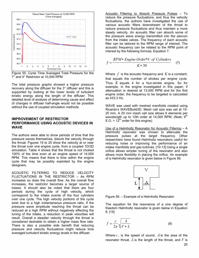
Figure 55 is the same plot as Figure 54, but extends the area ratio out to the diffuser exit to show the total pressure loss over the entire length. At 10,000 RPM the restrictors continue to lose total pressure over its entire length which surprisingly contrasts with a leveling off of total pressure for the same restrictors at 14,000 RPM.
20
Planar Mean Total Pressure at 10,000 RPM(Time Averaged)
95.4
95.8
96.2
96.6
97.0
97.4
97.8
98.2
98.6
99.0
1 2 3 4 5 6 7 8 9 10 11 12 13Normalized Area
Tota
l Pre
ssur
e [k
Pa]
7° 4°
Figure 55. Cycle Time Averaged Total Pressure for the 7° and 4° Restrictor at 10,000 RPM
The total pressure graphs showed a higher pressure recovery along the diffuser for the 3° diffuser and this is supported by looking at the lower levels of turbulent kinetic energy along the length of the diffuser. This detailed level of analysis of determining cause and effect of changes in diffuser half-angle would not be possible without the use of coupled simulation methods.
IMPROVEMENT OF RESTRICTOR PERFORMANCE USING ACOUSTIC DEVICES IN WAVE
The authors were able to show periods of time that the pressure waves themselves, disturb the velocity through the throat. Figures 19 to 25 show the velocity at or near the throat over one engine cycle, from a coupled 1D/3D simulation. Table 4 shows that the throat is not choked 100% of the time even at an engine speed of 14,000 RPM. This means that there is time within the engine cycle that may be possibly exploited by the engine designers.
ACOUSTIC FILTERING TO REDUCE VELOCITY FLUCTUATIONS IN THE RESTRICTOR – As RPM increases so does the overall flow. As the overall flow increases, the restrictor becomes a larger source of losses. It should also be noted that there are four periods during the cycle of high velocity, which correspond to the intake events of the four cylinders over one cycle. The high velocity portions of the cycle exist due to a high instantaneous pressure ratio. If the pressure wave amplitude reaching the throat can be reduced at a high RPM without negatively effecting the tuning of the intake, a reduction in peak velocities will result. Overall a steadier velocity through the throat is considered desirable to obtain a higher mass flow rate. There is also a possible side benefit that reducing pressure and velocity fluctuations might reduce time averaged turbulent kinetic energy levels in the diffuser.
Acoustic Filtering to Absorb Pressure Pulses – To reduce the pressure fluctuations, and thus the velocity fluctuations, the authors have investigated the use of various acoustic filters downstream of the throat to reduce pressure fluctuations and thus maintain a more steady velocity. An acoustic filter can absorb some of the pressure wave energy transmitted into the plenum from the intake valves. The frequency of each acoustic filter can be tailored to the RPM range of interest. The acoustic frequency can be related to the RPM point of interest by the following formula, Equation 7.
30*#
∗
∗=
KCylindersofOrderEngineRPM
f (7)
Where f is the acoustic frequency and K is a constant, that equals the number of strokes per engine cycle. Thus K equals 4 for a four-stroke engine. So for example, in the engine investigated in this paper, if attenuation is desired at 13,000 RPM and for the first engine order, the frequency to be targeted is calculated as 433.3 Hz.
WAVE was used with meshed manifolds created using Ricardo’s WAVEBuild3D. Mesh cell size was set at 15-20 mm. A 20 mm mesh cell size allows 6 elements per wavelength up to 12th order at 14,000 RPM. (Note: 6th E.O. = 12th order for this engine).
Use of a Helmholtz Resonator for Acoustic Filtering – A Helmholtz resonator was chosen to attenuate the pressure pulses at the target frequency. Other researchers have found Helmholtz resonators useful for reducing noise or improving the performance of an intake manifolds and gas turbines. [10-13] Using a single orifice allows simpler tuning of the resonator and also allows more flexibility in placing the orifice. An example of a Helmholtz resonator is given below in Figure 56.
Figure 56. – Example of a Helmholtz Resonator
The equation for the resonance of a one degree of freedom Helmholtz resonator is given below in Equation 8. [14]
LVAcf∗
=π2
(8)
Where c , is the speed of sound, A is the area of the resonator throat, L is the length of the throat, and V is
21
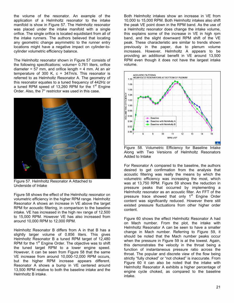
the volume of the resonator. An example of the application of a Helmholtz resonator to the intake manifold is show in Figure 57. The Helmholtz resonator was placed under the intake manifold with a single orifice. The single orifice is located equidistant from all of the intake runners. The authors believed that locating any geometric change asymmetric to the runner entry locations might have a negative impact on cylinder-to-cylinder volumetric efficiency balance.
The Helmholtz resonator shown in Figure 57 consists of the following specifications; volume= 0.761 liters, orifice diameter = 57 mm, and orifice length = 4 mm. At an air temperature of 300 K, c = 347m/s. This resonator is referred to as Helmholtz Resonator A. The geometry of this resonator equates to a tuned frequency of 442Hz or a tuned RPM speed of 13,260 RPM for the 1st Engine Order. Also, the 7° restrictor was used in this case.
Figure 57. Helmholtz Resonator A Attached to Underside of Intake
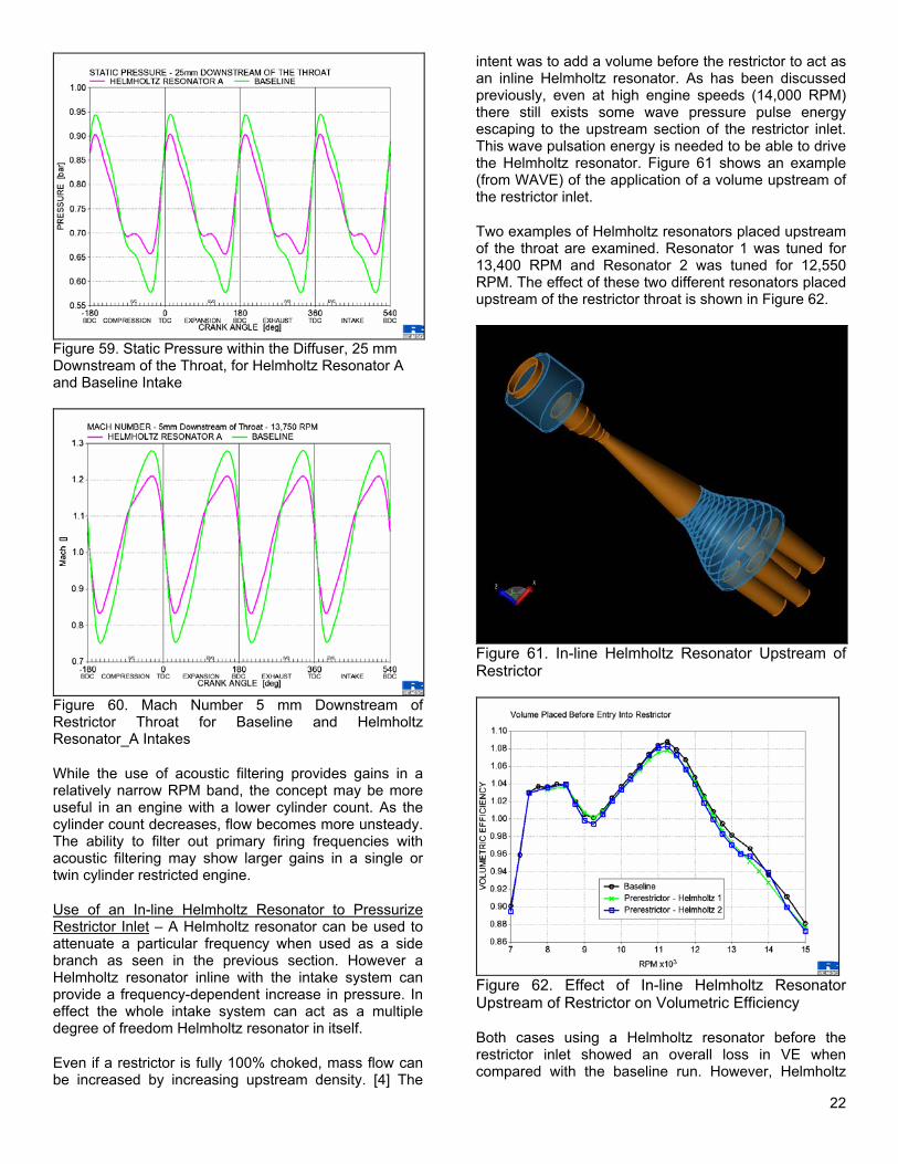
Figure 58 shows the effect of the Helmholtz resonator on volumetric efficiency in the higher RPM range. Helmholtz Resonator A shows an increase in VE above the target RPM for acoustic filtering, in comparison to the baseline intake. VE has increased in the high rev range of 12,500 to 15,000 RPM. However VE has also increased from around 10,000 RPM to 12,000 RPM.
Helmholtz Resonator B differs from A in that B has a slightly larger volume of 0.856 liters. This gives Helmholtz Resonator B a tuned RPM target of 12,480 RPM for the 1st Engine Order. The objective was to shift the tuned target RPM to a lower engine speed. However, it can be seen from Figure 58 that the same VE increase from around 10,000-12,000 RPM occurs, but the higher RPM increase appears different. Resonator A shows a bump in VE centered around 13,500 RPM relative to both the baseline intake and the Helmholtz B intake.
Both Helmholtz intakes show an increase in VE from 10,000 to 15,000 RPM. Both Helmholtz intakes also shift the peak VE point down in the RPM band. As the use of a Helmholtz resonator does change the intake volume, this explains some of the increase in VE in high rpm band, and the slight downward RPM shift of the VE peak. These characteristic are similar to trends shown previously in the paper, due to plenum volume increases. However, Helmholtz A appears to be providing an additional benefit in VE around 13,500 RPM even though it does not have the largest intake volume.
Figure 58. Volumetric Efficiency for Baseline Intake Along with Two Versions of Helmholtz Resonators Added to Intake
For Resonator A compared to the baseline, the authors desired to get confirmation from the analysis that acoustic filtering was really the means by which the volumetric efficiency was increasing the most, which was at 13,750 RPM. Figure 59 shows the reduction in pressure peaks that occurred by implementing a Helmholtz resonator as an acoustic filter. An FFT of the pressure trace showed that only 1st Engine Order content was significantly reduced. However there still existed pressure fluctuations from other higher order content.
Figure 60 shows the effect Helmholtz Resonator A had on Mach number. From the plot, the intake with Helmholtz Resonator A can be seen to have a smaller change in Mach number. Referring to Figure 59, it should be noted that the Mach number peaks occur when the pressure in Figure 59 is at the lowest. Again, this demonstrates the velocity in the throat being a function of instantaneous pressure ratio across the throat. The popular and discrete view of the flow being strictly “fully choked” or “not choked” is inaccurate. From Figure 60 it can also be noted that the intake with Helmholtz Resonator A exhibits a higher percentage of engine cycle choked, as compared to the baseline intake.
22
Figure 59. Static Pressure within the Diffuser, 25 mm Downstream of the Throat, for Helmholtz Resonator A and Baseline Intake
Figure 60. Mach Number 5 mm Downstream of Restrictor Throat for Baseline and Helmholtz Resonator_A Intakes
While the use of acoustic filtering provides gains in a relatively narrow RPM band, the concept may be more useful in an engine with a lower cylinder count. As the cylinder count decreases, flow becomes more unsteady. The ability to filter out primary firing frequencies with acoustic filtering may show larger gains in a single or twin cylinder restricted engine.
Use of an In-line Helmholtz Resonator to Pressurize Restrictor Inlet – A Helmholtz resonator can be used to attenuate a particular frequency when used as a side branch as seen in the previous section. However a Helmholtz resonator inline with the intake system can provide a frequency-dependent increase in pressure. In effect the whole intake system can act as a multiple degree of freedom Helmholtz resonator in itself.
Even if a restrictor is fully 100% choked, mass flow can be increased by increasing upstream density. [4] The
intent was to add a volume before the restrictor to act as an inline Helmholtz resonator. As has been discussed previously, even at high engine speeds (14,000 RPM) there still exists some wave pressure pulse energy escaping to the upstream section of the restrictor inlet. This wave pulsation energy is needed to be able to drive the Helmholtz resonator. Figure 61 shows an example (from WAVE) of the application of a volume upstream of the restrictor inlet.
Two examples of Helmholtz resonators placed upstream of the throat are examined. Resonator 1 was tuned for 13,400 RPM and Resonator 2 was tuned for 12,550 RPM. The effect of these two different resonators placed upstream of the restrictor throat is shown in Figure 62.
Figure 61. In-line Helmholtz Resonator Upstream of Restrictor
Figure 62. Effect of In-line Helmholtz Resonator Upstream of Restrictor on Volumetric Efficiency
Both cases using a Helmholtz resonator before the restrictor inlet showed an overall loss in VE when compared with the baseline run. However, Helmholtz
23
resonator 2 does show a relative bump in VE slightly above the tuned target of 13,400 RPM. In this case, any pressure gains at a particular frequency are offset by losses across the RPM band.
INVESTIGATION OF A FLOW CONTROL DEVICE USING WAVE-VECTIS
To reduce the onset of separation a flow control device was placed upstream of the throat in the inlet section. The device uses four swirl vanes to induce a swirl in the flow (i.e. induce a tangential velocity component) about the main restrictor axis. Inducing swirl is intended to impart radial momentum to the flow downstream of the throat.
SWIRL GENERATION UPSTREAM OF THE THROAT – Previous work by Gaiser et al [15], showed inducing swirl into the flow by the use of turning vanes upstream of a diffuser can reduce separation losses, with gains in the diffuser outweighing the losses from the vanes.
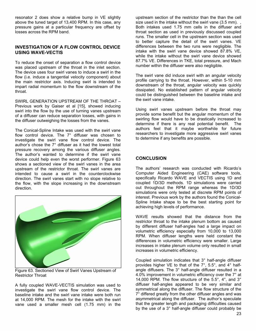
The Conical-Spline Intake was used with the swirl vane flow control device. The 7° diffuser was chosen to investigate the swirl vane flow control device. The author’s chose the 7° diffuser as it had the lowest total pressure recovery among the various diffuser angles. The author’s wanted to determine if the swirl vane device could help even the worst performer. Figure 63 shows a sectioned view of the swirl vanes in the area upstream of the restrictor throat. The swirl vanes are intended to cause a swirl in the counterclockwise direction. The swirl vanes start with no slope relative to the flow, with the slope increasing in the downstream direction.
Figure 63. Sectioned View of Swirl Vanes Upstream of Restrictor Throat
A fully coupled WAVE-VECTIS simulation was used to investigate the swirl vane flow control device. The baseline intake and the swirl vane intake were both run at 14,000 RPM. The mesh for the intake with the swirl vane used a smaller mesh cell (1.75 mm) in the
upstream section of the restrictor than the than the cell size used in the intake without the swirl vane (3.5 mm). , Both intakes used 1.75 mm cells in the diffuser and throat section as used in previously discussed coupled runs. The smaller cell in the upstream section was used to better capture the detail of the swirl vanes. VE differences between the two runs were negligible. The intake with the swirl vane device showed 87.8% VE, while the intake without the swirl vane device showed 87.7% VE. Differences in TKE, total pressure, and Mach number within the diffuser were also negligible.
The swirl vane did induce swirl with an angular velocity profile carrying to the throat. However, within 5-10 mm downstream of the throat, angular velocity was quickly dissipated. No established pattern of angular velocity could be distinguished between the baseline intake and the swirl vane intake.
Using swirl vanes upstream before the throat may provide some benefit but the angular momentum of the swirling flow would have to be drastically increased to determine if there is any real potential benefit. The authors feel that it maybe worthwhile for future researchers to investigate more aggressive swirl vanes to determine if any benefits are possible.
CONCLUSION
The authors’ research was conducted with Ricardo’s Computer Aided Engineering (CAE) software tools, specifically Ricardo WAVE and VECTIS using 1D and coupled 1D/3D methods. 1D simulations were carried out throughout the RPM range whereas the 1D/3D simulations were only tested at discrete RPM points of interest. Previous work by the authors found the Conical-Spline Intake shape to be the best starting point for achieving high levels of performance.
WAVE results showed that the distance from the restrictor throat to the intake plenum bottom as caused by different diffuser half-angles had a large impact on volumetric efficiency especially from 10,000 to 13,000 RPM. When diffuser lengths were held constant the differences in volumetric efficiency were smaller. Large increases in intake plenum volume only resulted in small increases in volumetric efficiency.
Coupled simulation indicates that 3° half-angle diffuser provides higher VE to that of the 7°, 5.5°, and 4° half-angle diffusers. The 3° half-angle diffuser resulted in a 4.0% improvement in volumetric efficiency over the 7° at 14,000 RPM. The flow structure of the 5.5°, 4°, and 3° diffuser half-angles appeared to be very similar and symmetrical along the diffuser. The flow structure of the 7° differed greatly from the other diffuser angles and was asymmetrical along the diffuser. The author’s speculate that the greater length and packaging difficulties caused by the use of a 3° half-angle diffuser could probably be
24
overcome by a transition of the diffuser exit to the main plenum volume at a diffuser area ratio of around 8. The authors found very little difference in total pressure (and static pressure) at area ratios greater than 8.
Above 12,000 RPM, WAVE results tended to predict values of VE greater than the theoretical analysis based on compressible fluid flow equations and simplifying assumptions. WAVE-VECTIS prediction gave much better agreement with theoretical analysis. In some cases WAVE-VECTIS VE predictions were slightly greater than theoretical prediction. This is believed to be caused by the difference in the definition of the VE used between analysis and simulation. In the analysis, volumetric efficiency was defined from the reference of the throat. In the simulation and in practice it is the flow through the valves in the cylinder that is measured when calculating the volumetric efficiency.
It has also been shown that while various factors can determine restrictor performance and how it interacts with the engine tuning, that the diffuser angle is the largest factor in effecting volumetric efficiency gains, even at mid-range RPM.
The restrictor is not choked 100% of the time, even at high engine speeds. The percentage of the cycle choked varied with RPM and with the diffuser half-angle. At 10,000 RPM the 7deg restrictor was choked 0% of the cycle, while the 4deg restrictor was choked 15.3% of the cycle. At 14,000 RPM the amount of the time the throat was choked varied from 47.9% to 83.3% of the complete cycle. Percentage of cycle choked increased as diffuser half-angle decreased at both 10,000 and 14,000 RPM. Increased percentage of cycle choked correlated with increased VE in all instances. Tighter diffuser angles also had a more uniform Mach number distribution at a given cross-section than wider angles.
Tighter diffuser half-angles had lower levels of turbulent kinetic energy and smaller loss of total pressure. Turbulent kinetic energy peaks shortly after the time at which velocities in the diffuser peak. Rises in total pressure are believed to be caused by large pressure pulses and also due to errors introduced by the use of area averaging method in VECTIS when applied to non-uniform flows. Total pressure rise due to numeric error seems less likely as pressure rise occurred even at subsonic velocities downstream of the throat.
The use of acoustic filtering methods using Helmholtz resonators to make flow at the restrictor throat more uniform and regular appeared promising. A Helmholtz resonator inside the plenum damped velocity fluctuations at the throat and offered improvements in VE at high engine speeds. VE increased at the tuned rpm point for one intake by approximately 2% over the expected increase provided by just the additional plenum volume. A Helmholtz resonator placed inline and upstream of the restrictor throat showed VE losses at mid to high RPM. A disadvantage of the resonators is
that their benefit is highly sensitive to differences in geometry and tuned RPM point.
The use of swirl inducing vanes upstream of the restrictor throat provided no benefit in terms of volumetric efficiency improvement. Any swirl generated by the vanes was quickly dampened out downstream of the throat. However, more aggressive swirl vanes might prove more promising and should be considered in future research.
ACKNOWLEDGMENTS
Special thanks go to our original team advisor Dr. Patrick Starr for initially sponsoring the research work and to Dr. David Kittleson and Dr. William Durfee for continuing their support and sponsorship of our research. The authors also thank Garrett Stockburger for his advice and support. The authors would also like to acknowledge the continual assistance of Dr. Birali Runesha and the rest of the support staff at the Minnesota Supercomputing Institute for their help in high performance computing. We would like to thank Ricardo Software and in particular Karl John, Patrick Niven, and Enrico Bradamante for their generous support and advice. We would also like to thank Kim Lyon of Daimler-Chrysler for his expertise and advice regarding engine modeling and calibration. Additional thanks goes to Dr. Bruce Jones of Mankato State University for allowing us to use his department’s flow bench. We would like to thank team members John Kess and Aaron Reinhart for helping us make test fixtures and gather data for the team’s WAVE models.
REFERENCES
1. Society of Automotive Engineers, “2006 Formula SAE Rules”, http://www.sae.org/students/fsaerules.pdf (31 May 2006).
2. Claywell, M. R., Horkheimer, D. P., and Stockburger, G. R., “Investigation of Intake Concepts for Formula SAE Four-Cylinder Engine Using 1D/3D (Ricardo WAVE-VECTIS) Coupled Modeling Techniques”, SAE 2006 Motorsports Conference, 2006-01-3652.
3. Guizzetti, M. and Colombo, T. “Combined WAVE-VECTIS Simulation of an Intake Manifold of V6 PFI Gasoline Engine”, http://www.ricardo.com/download/pdf/VECTIS_combined_wave_VECTIS.pdf (31 May 2006).
4. Saad, M. A., Compressible Fluid Flow, 2nd Edition, Prentice Hall, 1993, ISBN 0-13-161373-1.
5. Bressler, H., Rammoser, D., Neumaier, H., Terres, F., “Experimental and Predictive Investigation of a Close-Coupled Catalytic Converter with Pulsating Flow”, SAE 960564.
25
6. Issa, R. I., “Rise of Total Pressure in Frictional Flow”, AIAA Journal 1995, Vol. 33, No. 4, pp. 772-774.
7. Homann, F., “The Effect of High Viscosity on the Flow Around a Cylinder and Around A Sphere”, NACA-TM-1334.
8. Wyatt, D. D., “Analysis of Errors Introduced By Several Methods of Weighting Non-Uniform Duct Flow”, NACA-TN-3400, 1955.
9. Pianko, M. and Wazelt, F., Suitable Averaging Techniques in Non-Uniform Internal Flow, Propulsion and Energetics Panel Working Group 14, AGARD-AR-182, 1983.
10. Dupère, I. D. J., and Dowling, A. P., “The Use of Helmholtz Resonators in a Practical Combustor”, Journal of Engineering for Gas Turbines and Power, April 2005, Vol. 127, pp. 268-275.
11. Onorati, A., Montenegro, G., and Errico, G. D., “Prediction of the Attenuation Characteristics of I.C. Engine Silencers by 1-D and Multi-D Simulation Models”, SAE 2006-01-1541.
12. Wan, D., and Soedel, D. T., “Two Degree of Freedom Helmholtz Resonator Analysis”, SAE 2004-01-0387.
13. Selamet, A., Dickey, N. S., Radavich, P. M., and Novak, J. M., “Theoretical, Computational and Experimental Investigation of Helmholtz Resonators: One-Dimensional Versus Multi-Dimensional Approach”, SAE 940612.
14. Winterborne, D., and Pearson, R., Design Technologies for Engine Manifolds – Wave Action Methods for IC Engines, 1999.
15. Gaiser, G., Oesterle, J., Braun, J., and Zacke, P., “The Progressive Spin Inlet – Homogenous Flow Distributions Under Stringent Conditions”, SAE 2003-01-0840.
CONTACT
Mark R. Claywell has a Bachelor in Mechanical Engineering from the University of Minnesota. [email protected]
Donald P. Horkheimer has a Bachelor in Aerospace Engineering and Mechanics from the University of [email protected] http://www.me.umn.edu/~hork0004
DEFINITIONS, ACRONYMS, ABBREVIATIONS
CAD: Computer Aided Design or Crankangle Degrees
CAE: Computer Aided Engineering
CFD: Computational Fluid Dynamics
FFT: Fast Fourier Transform
RPM: Revolutions per Minute
TKE: Turbulent Kinetic Energy
VE: Volumetric Efficiency
NOMENCLATURE
General
A Area [m2]
xA Area at Distance from Throat [m2]
∗A Area at Restrictor Throat [m2]
c Speed of Sound [m/s]
f Frequency [Hz]
γ Ratio of Specific Heats
v
p
CC
K Engine Stroke Constant [4]
L Length [m]
φ Arbitrary Scalar -
ψ Flow Uniformity Index -
P Pressure [Pa]
ρ Density [kg/m3]
Q& Volumetric Flow Rate [m3/s]
V Volume [m3]
Subscripts
0 Stagnation Conditions
i Scalar at a Mesh Cell in a Plane
mean Average Scalar Value across a Plane

![FIA 10/05/01 - Motorsports Association · Web viewInjection :Make: Type: [e] If an air restrictor is fitted, diameter of the restrictor: mm [f] If supercharged, is the supercharger](https://static.fdocuments.in/doc/165x107/5ad61a727f8b9a5d058e07a0/fia-100501-motorsports-association-viewinjection-make-type-e-if-an-air.jpg)