IMPROVEMENT AND DEVELOPMENT OF HIGH-FREQUENCY WIRELESS TOKEN-RING PROTOCOL

A THESIS SUBMITTED TO THE GRADUATE SCHOOL OF NATURAL AND APPLIED SCIENCES

OF MIDDLE EAST TECHNICAL UNIVERSITY

BY

TANER KURTULUŞ

IN PARTIAL FULFILLMENT OF THE REQUIREMENTS FOR

THE DEGREE OF MASTER OF SCIENCE IN

COMPUTER ENGINEERING

DECEMBER 2010

Approval of the thesis:

IMPROVEMENT AND DEVELOPMENT OF HIGH-FREQUENCY WIRELESS TOKEN-RING PROTOCOL

submitted by TANER KURTULUŞ in partial fulfillment of the requirements for the degree of Master of Science in Computer Engineering Department, Middle East Technical University by, Prof. Dr. Canan Özgen _____________________ Dean, Graduate School of Natural and Applied Sciences Prof. Dr. Adnan Yazıcı _____________________ Head of Department, Computer Engineering Inst. Dr. Cevat Şener _____________________ Supervisor, Computer Engineering Dept., METU Examining Committee Members: Assoc. Prof. Dr. Ahmet Coşar _____________________ Computer Engineering Dept., METU Inst. Dr. Cevat Şener _____________________ Computer Engineering Dept., METU Inst. Dr. Atilla Özgit _____________________ Computer Engineering Dept., METU Inst. Dr. Onur Tolga Şehitoğlu _____________________ Computer Engineering Dept., METU Özgür Özuğur , M.Sc. _____________________ UEKAE, TÜBİTAK-BILGEM Date: 15/12/2010

iii

I hereby declare that all information in this document has been obtained and presented in accordance with academic rules and ethical conduct. I also declare that, as required by these rules and conduct, I have fully cited and referenced all material and results that are not original to this work. Name, Last name : Taner KURTULUŞ Signature :

iv

ABSTRACT

IMPROVEMENT AND DEVELOPMENT OF HIGH-FREQUENCY WIRELESS TOKEN-RING PROTOCOL

KURTULUŞ, Taner M.Sc., Department of Computer Engineering Supervisor : Dr. Cevat ŞENER

December 2010, 72 pages

STANAG 5066 Edition 2 is a node-to-node protocol developed by NATO in order to

communicate via HF media. IP integration is made to be able to spread the use of

STANAG 5066 protocol. However, this integration made the communication much

slower which is already slow. In order to get faster the speed and communicate

within single-frequency multi-node network, HFTRP, which is a derivative of

WTRP, is developed. This protocol is in two parts, first is a message design for

management tokens exchanged by communicating nodes, and second is the

algorithms used to create, maintain, and repair the ring of nodes in the network.

Scope of this thesis is to find out a faster ring setup, growing procedure and to

implement. Beside, finding optimum values of tuning parameters for HFTRP is also

in the scope of this thesis.

Keywords: Wireless Token Ring Protocol, Medium Access Protocol, Medium

Access Protocol Implementation, STANAG 5066, High Frequency Data-Link

Protocol

v

ÖZ

YÜKSEK FREKANSTA SİMGELİ HALKA PROTOKOLÜNÜN (HFTRP) GELİŞTİRİMİ VE GERÇEKLEŞTİRİMİ

KURTULUŞ, Taner Yüksek Lisans, Bilgisayar Mühendisliği Bölümü Tez Yöneticisi : Dr. Cevat ŞENER

Aralık 2010, 72 sayfa

STANAG 5066 Edition 2 yüksek frekanslı ortamlarda kullanılmak üzere NATO

tarafından geliştirilen noktadan noktaya iletişim sağlayan bir protokoldür. Bu

protokolün daha çok yerde kullanılabilmesi için IP ile entegre hale getirilmiştir.

Fakat bu entegrasyon çok yavaş olan haberleşmeyi daha da yavaş hale getirmiştir.

Haberleşme hızını arttırabilmek için ve tek frekansta çok nokta arasında iletişimi

sağlamak için bir WTRP türevi olan HFTRP geliştirilmektedir. Bu protokol iki

kısımdan oluşur; biri terminaller arası kullanılacak yönetim simgelerinin tasarımı,

ikincisi de iletişim ortamının yaratılması, bakımı ve düzeltilmesi için kullanılacak

algoritmalardır. Bu tezde bizim amacımız, yavaş olan halka oluşturma, halkaya

katılma işlemlerini hızlandırmak ve gerçekleştirmektir. Bunlara ek olarak ayar

parametrelerinin en uygun değerleri bulmaktır.

Anahtar Kelimeler: Kablosuz Token Ring Protokol, Ortam Erişim Protokolü,

Ortam Erişim Protokolü Gerçekleştirimi, STANAG 5066, Yüksek Frekansta Veri-

Bağlantı Katmanı Protokolü

vi

To My Family

vii

ACKNOWLEDGMENTS

First of all, I would like to express my sincere thanks to my supervisor, Dr. Cevat

ŞENER for his efforts and guidance throughout this thesis work.

I must also acknowledge my project manager, Özgür Özuğur, for encouraging

me on this research topic and his continuous support.

I would also like to thank my collages, especially E. Serdar Ayaz for helping me on

bug fixing of code, and all my friends not named for their support during my M.Sc.

A very special thanks goes to my wife for her support and patience.

In conclusion, I recognize that this research would not have been possible

without the support of my employer, TÜBİTAK-BILGEM/UEKAE.

viii

TABLE OF CONTENTS

ABSTRACT............................................................................................................................iv 

ÖZ.............................................................................................................................................v 

ACKNOWLEDGMENTS ................................................................................................... vii 

TABLE OF CONTENTS ................................................................................................... viii 

LIST OF TABLES ..................................................................................................................x 

LIST OF FIGURES ...............................................................................................................xi 

LIST OF ABBREVIATIONS ............................................................................................ xiii 

CHAPTERS

1. INTRODUCTION...............................................................................................................1 

2. BACKGROUND AND LITERATURE ............................................................................4 

2.1  HF Communications..................................................................................................4 2.1.1  HF at Military Communications ..................................................................................... 4 2.1.2  HF Propagation ............................................................................................................... 4 2.1.3  Interleaving ..................................................................................................................... 5 2.1.4  HF Bandwidth Limitation ............................................................................................... 6 2.1.5  HF Standardizations ........................................................................................................ 7 

2.2  Protocols ....................................................................................................................8 2.2.1  Wireless Token Ring Protocol ........................................................................................ 8 2.2.2  Token Ring Protocol ....................................................................................................... 8 2.2.3  HFTRP ............................................................................................................................ 9 

2.3  Related Work...........................................................................................................10 

3. HIGH FREQUENCY TOKEN RING PROTOCOL DESCRIPTION........................12 

3.1  Definitions ...............................................................................................................12 3.2  Token Specification and Token Types ....................................................................13 3.3  State Machine Specification ....................................................................................20 3.1  Timers......................................................................................................................21 

3.1.1  Calculation of Timers.................................................................................................... 25 3.1.2  Scalar Tuning Parameters ............................................................................................. 27 

ix

3.2  General Scenarios....................................................................................................28 3.2.1  Normal Ring Operations ............................................................................................... 28 3.2.2  Self-Ring and Ring Creation......................................................................................... 30 3.2.3  Joining to Ring .............................................................................................................. 31 3.2.4  Relaying Operation ....................................................................................................... 32 

4. PROPOSED IMPROVEMENTS ON HFTRP...............................................................35 

4.1  Scalar Tuning Parameter Values .............................................................................35 4.1.1  MAX_NUM_STATIONS............................................................................................. 35 4.1.2  CYCLE_PER_SOLICITATION................................................................................... 35 4.1.3  Slot Sizes....................................................................................................................... 36 4.1.4  Number of Slots ............................................................................................................ 38 4.1.5  IDLE_WAIT_TIME ..................................................................................................... 39 4.1.6  SUCCR_WAIT_TIME ................................................................................................. 39 4.1.7  CONTENTION_WAIT_TIME..................................................................................... 40 4.1.8  TOKEN_PASS_WAIT_TIME ..................................................................................... 40 4.1.9  MODEM_LATENCY_DELTA.................................................................................... 41 

4.2  EOT Calculation......................................................................................................41 4.3  State Machine Changes ...........................................................................................43 

5. IMPLEMENTATION AND SIMULATION .................................................................47 

5.1  Implementation Language .......................................................................................47 5.2  Target Operating System.........................................................................................47 5.3  State Machine Implementation................................................................................48 5.4  Simulator .................................................................................................................54 

6. TEST RESULTS ...............................................................................................................57 

6.1  Real Environment Tests ..........................................................................................57 6.2  Simulator Tests........................................................................................................59 

6.2.1  Ring Formation ............................................................................................................. 59 6.2.2  Latency Tests ................................................................................................................ 61 6.2.3  Throughput Tests .......................................................................................................... 66 6.2.4  Robustness Test of Ring Formation.............................................................................. 67 

7. CONCLUSION .................................................................................................................69 

REFERENCES......................................................................................................................71 

x

LIST OF TABLES

TABLES

Table 1 - WTRP Frame Fields Descriptions .............................................................. 14 

Table 2 - EOW-HFTRP-Token Message [13] ........................................................... 16 

Table 3 - RTT token fields values.............................................................................. 17 

Table 4 – ACK Token Fields Values ......................................................................... 17 

Table 5 - SLS Token Fields Values ........................................................................... 18 

Table 6 - SET Token Fields Values ........................................................................... 19 

Table 7 - REL Token Fields Values........................................................................... 19 

Table 8 - Delete Token Fields Values........................................................................ 20 

Table 9 - HFTRP States and Their Descriptions........................................................ 22 

Table 10 - Timers and Descriptions ........................................................................... 24 

Table 11 - Timers' Default Values ............................................................................. 25 

Table 12 - Scalar Tuning Parameters and Default Values ......................................... 27 

Table 13 – Improved-HFTRP FLT State Transition Table........................................ 44 

Table 14 – Outbound Transition Table of ILDE State [7] ......................................... 49 

Table 15 - Method Descriptions................................................................................. 52 

Table 16 - Latency values for 3 nodes for 1000 sec .................................................. 61 

Table 17 - Latency values for 6 nodes for 1000 sec .................................................. 63 

Table 18 - Throughput Comparison........................................................................... 67 

xi

LIST OF FIGURES

FIGURES

Figure 1 - HF Propagation Paths [4] ............................................................................ 5 

Figure 2 - Interleaver and Deinterleaver[6] ................................................................. 6 

Figure 3 - WTRP Frame Format ................................................................................ 14 

Figure 4 - State Overviews and Transitions............................................................... 23 

Figure 5 - Normal Ring Operation ............................................................................. 29 

Figure 6 - States of Normal Ring Operation .............................................................. 29 

Figure 7 - Ring Creation Operation ........................................................................... 30 

Figure 8 - Joining Operation ...................................................................................... 31 

Figure 9 - States of Joining Ring Operation .............................................................. 32 

Figure 10 - States of Creating Ring Operation .......................................................... 33 

Figure 11 – Relaying Operation................................................................................. 34 

Figure 12 - Sates of Relaying operation..................................................................... 34 

Figure 13 - Choosing Slot .......................................................................................... 37 

Figure 14 - HF Communication Environment ........................................................... 42 

Figure 15 – Improved-HFTRP Ring Creation States................................................. 43 

Figure 16 – Improved-HFTRP State Transitions ....................................................... 45 

Figure 17 - Design of State Pattern ............................................................................ 50 

Figure 18 - HFTRP State Methods ............................................................................ 51 

Figure 19 - Code Sample of HFTRP.......................................................................... 53 

Figure 20 - State Pattern with Methods ..................................................................... 53 

Figure 21 - Change State Method .............................................................................. 54 

Figure 22 – Node and Nic Contents........................................................................... 55 

Figure 23 - Scenerio Planning Example .................................................................... 56 

xii

Figure 24 - Real Environment Scenario..................................................................... 57 

Figure 25 - Real Environment Test Results ............................................................... 58 

Figure 26 - Simulation Results for 3-node at Ideal Channel...................................... 59 

Figure 27 - Simulation Results for 6-node at Ideal Channel...................................... 60 

Figure 28 - Packet Latency on 3 nodes for 1000s...................................................... 62 

Figure 29 - Packet Latency on 6 nodes for 1000s...................................................... 63 

Figure 30 - Packet Latency on 3-node for 10000 sec................................................. 64 

Figure 31 - Packet Latency on 6-node for 10000 sec................................................. 64 

Figure 32 - Packet Latency on 3 nodes after ring formation...................................... 65 

Figure 33 - Packet latency on 6 nodes after ring formation....................................... 65 

Figure 34 - Change of ring size in one billion seconds of time period ...................... 68 

xiii

LIST OF ABBREVIATIONS

ANSI American National Standards Institute

BLOS Beyond Line of Side BPS Bits Per Second

CSMA Carrier Sense Multiple Access DCE Data Communication Equipment

DTE Data Terminal Equipment EOT End of Transmission

FEC Future Error Correction FED-STD Federal Standard HF High Frequency HFTRP High Frequency Wireless Token Ring Protocol

IDE Integrated Development Environment IEEE Institute of Electrical and Electronics Engineers ISO International Organization for Standardization LAN Local Area Network

LOS Line of Side MAC Medium Access Control

MIL-STD Military Standards NATO North Atlantic Treaty Organization

OSI Open Systems Interconnection PDU Protocol Data Unit

POSIX Portable Operating System Interface [for UNIX] QoS Quality of Service

STANAG Standardization Agreement TDMA Time Division Multiple Access

WTRP Wireless Token Ring Protocol

1

CHAPTER 1

1. INTRODUCTION

High frequency (HF) communications has been an integral part of worldwide

information transmission since the dawn of radio and kept pace with the information

age [7]. Radio waves, which have frequency between 3 MHz and 30 MHz, are called

HF. This frequency attribute gives special characteristics for reflection and

propagation. Main characteristic is reflecting from ionosphere. In fact, there is no

other frequency range that has ability to reflect from ionosphere. Therefore, only HF

radio waves give opportunity of communicating beyond line of side without using

any repeaters. Some military and industrial standards have been developed to use this

communication path more effectively.

One of NATO standards is STANAG 5066 Ed2, which is a point-to-point protocol,

for HF medium. In the operational scenarios, the need of communicating with more

than one station has occurred. This can be achieved by some methods. One of this is

using more then one radio for each communication between other stations. When

using this approach, extra effort is needed on planning frequencies between stations

and other effort is planning locations of radios to prevent interference.

Other approach is communicating at single broadcast frequency. However, this

approach has some difficulties originated from wireless communication.

Programming can solve these difficulties. There is no need of extra planning on

hardware, no extra estimation for preventing interference.

Since HF has limited bandwidth and open to burst errors, some other solutions has

needed other than regular wireless protocols, such as IEEE 802.5, IEEE 802.11. One

solution is to add more functionality to STANAG 5066 Ed2. NATO has chosen this

2

approach and developed Edition 3 of STANAG 5066. Edition 3 has three MAC layer

protocols. These are HF CSMA, HFTRP, HF TDMA. But, HF TDMA has not

developed yet.

Although, HFTRP has much more bandwidth utilization than HF CSMA, HFTRP

has some weaknesses. One of the weaknesses is need of a ring creation. This means,

to operate in a stable state there is need of some pre-work on the ring. Thus, some

initial time takes to get ready for operating. Also, while growing the ring when

inviting others some more time is used without data transmission. These parts should

be improved and waiting timers should be optimized.

In this thesis, improvements to the ring creation and growing algorithms will be

explained. In which scenarios, proposed improvements have valuable effects than

regular HFTRP will be examined. Beside this, optimum values to some tuning

parameters will be studied and at the end implementation details and methods will be

explained.

Since the need of proofing the improvements, simulation technique and tests on real

environment methods are used. For simulation environment OMNeT++ open

simulator [15] that is an open source discrete event network simulator has been used.

In the real environment, Marconi radios and RapidM RM6 modems have been used

as a physical layer. What are the improvements and results will be explained at the

next chapters.

The rest of this thesis proceeds as follows. In Chapter 2, background information

about High Frequency communications is given. Chapter 3 reminds the necessary

background on High Frequency Token Ring Protocol and description of that

protocol. In Chapter 4, the tunings and improvements proposed to enhance the

HFTRP are explained. Chapter 5 defines the simulation and the implementation

details of HFTRP, where a new approach to protocol implementation has been given.

Chapter 6 defines the test results of original HFTRP and Improved-HFTRP.

3

Performance comparisons of these two protocols also have been discussed in this

chapter. Finally, Chapter 7 concludes the thesis work according to test results and

also states future work.

4

CHAPTER 2

2. BACKGROUND AND LITERATURE

In this chapter, high frequency communications, protocols, some concepts that are

used in HF domain and related studies are explained.

2.1 HF Communications

Advantages and disadvantages of HF have been discussed here. However HF has

difficulties, solutions for those difficulties have been found and some are explained

here.

2.1.1 HF at Military Communications

HF has the ability to communicate across long distances without the use of repeaters

or satellites because of its various modes of propagation. This ability has a large

utility in the military arena where ad hoc communications are required with minimal

assets and planning.[16] Furthermore, satellites are more open to attacks or sniffing

than HF.

2.1.2 HF Propagation

Propagation defines how radio waves radiate from transmitting source. It is believed

that radio waves propagate like a straight line. However it is a bit complicated. There

are two basic modes of propagation. These are ground waves and sky waves. As their

names imply ground waves travel along the surface of ground and sky waves after

reflecting from ionosphere return to ground. Simply, Figure 1 shows propagation

paths of HF radio waves. Sky waves are not formed other than HF waves, because

reflecting from ionosphere strictly dependent on frequency of radio waves. As a

consequence, sky waves of HF give opportunity to communicate beyond line of side.

5

While communicating long distances, signals are interfered with others or burst

errors are occurred. Consequently, some error correction methods have been used in

HF communications. Such as, interleaving, coding, etc.

Figure 1 - HF Propagation Paths [4]

2.1.3 Interleaving

Interleaving is frequently used in digital communication and storage systems to

improve the performance of FEC codes. Errors typically occur in burst rather than

independently in wireless channels. If the number of errors within a code word

exceeds the error-correcting code's capability, it fails to recover the original code

word. Interleaving overcomes this problem by shuffling source symbols across

several code words, thereby creating a more homogenous error. [18]

6

However, use of interleaving techniques helps error correction, it increases latency.

This is because the entire interleaved block must be buffered before sending to

channel and must be received before the packets can be decoded. [18]

Figure 2 - Interleaver and Deinterleaver[6]

2.1.4 HF Bandwidth Limitation

Nyquist’s Bit Rate theorem is used to calculate maximum channel capacity at non-

noisy media in terms of bps. Nyquist’s Bit Rate Theorem [14];

C = 2 x B x log2M bits/sec (1) where;

C: Channel Capacity

B: Bandwidth

M: Number of signal levels used.

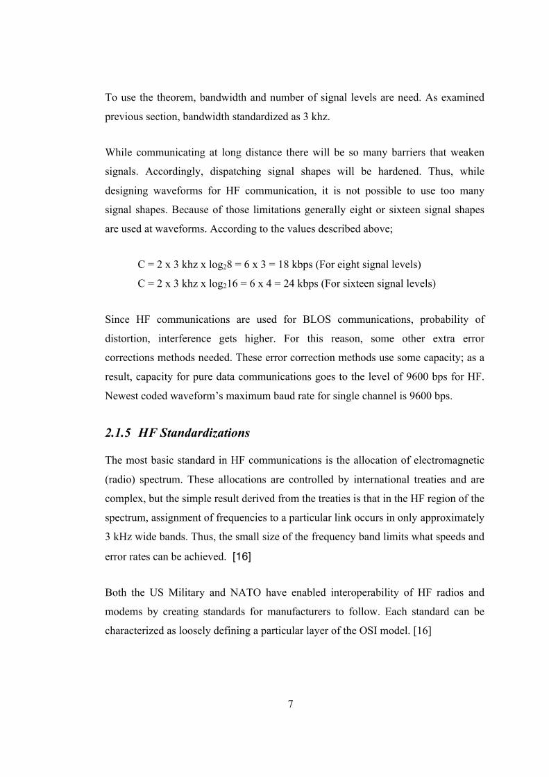
7

To use the theorem, bandwidth and number of signal levels are need. As examined

previous section, bandwidth standardized as 3 khz.

While communicating at long distance there will be so many barriers that weaken

signals. Accordingly, dispatching signal shapes will be hardened. Thus, while

designing waveforms for HF communication, it is not possible to use too many

signal shapes. Because of those limitations generally eight or sixteen signal shapes

are used at waveforms. According to the values described above;

C = 2 x 3 khz x log28 = 6 x 3 = 18 kbps (For eight signal levels)

C = 2 x 3 khz x log216 = 6 x 4 = 24 kbps (For sixteen signal levels)

Since HF communications are used for BLOS communications, probability of

distortion, interference gets higher. For this reason, some other extra error

corrections methods needed. These error correction methods use some capacity; as a

result, capacity for pure data communications goes to the level of 9600 bps for HF.

Newest coded waveform’s maximum baud rate for single channel is 9600 bps.

2.1.5 HF Standardizations

The most basic standard in HF communications is the allocation of electromagnetic (radio) spectrum. These allocations are controlled by international treaties and are complex, but the simple result derived from the treaties is that in the HF region of the

spectrum, assignment of frequencies to a particular link occurs in only approximately

3 kHz wide bands. Thus, the small size of the frequency band limits what speeds and

error rates can be achieved. [16]

Both the US Military and NATO have enabled interoperability of HF radios and modems by creating standards for manufacturers to follow. Each standard can be characterized as loosely defining a particular layer of the OSI model. [16]

8

There are 3 major standards bodies for tactical HF communications. These are: the

US Military with the MIL-STD series, NATO with its STANAG (standardization) documents and the US Federal Government with the FED-STD series. [16]

This thesis focuses on STANAG standards and specially STANAG 5066 Edition 3.

Description of STANAG 5066 is “Profile for High Frequency (HF) Radio Data

Communication”. This standard covers all layers of OSI reference model. However,

this thesis will focus on one subsection of MAC layer. It is HFTRP.

2.2 Protocols

In this section some information about protocols used in HF or base protocols are

given.

2.2.1 Wireless Token Ring Protocol

Wireless Token Ring protocol is the base protocol of HF Token Ring Protocol.

Which is a robust, self-healing, self-coordinating and distributed MAC layer protocol

for ad-hoc networks. The MAC protocol through which mobile stations can share a

common broadcast channel is essential in an ad-hoc network. Due to the existence of

hidden terminals and partially connected network topology, contention among

stations in an ad-hoc network is not homogeneous. Some stations can suffer severe

throughput degradation in access to the shared channel when load of the channel is

high, which also results in unbounded medium access time for the stations. This

challenge is addressed as quality of service (QoS) in a communication network. [3]. The idea behind WTRP is token ring protocol, which is used at wired networks.

2.2.2 Token Ring Protocol

Token Ring is a LAN protocol defined in the IEEE 802.5 where all stations are

connected in a ring and each station can directly hear transmissions only from its

9

immediate neighbor. Permission to transmit is granted by a message (token) that

circulates around the ring.

Token-passing networks move a small frame, called a token, around the network.

Possession of the token grants the right to transmit. While the information frame is

circling the ring, no token is on the network, which means that other stations wanting

to transmit must wait. Therefore, collisions cannot occur in Token Ring networks.

Unlike Ethernet CSMA/CD networks, token-passing networks are deterministic,

which means that it is possible to calculate the maximum time that will pass before

any end station will be capable of transmitting. This feature and several reliability

features make Token Ring networks ideal for applications in which delay must be

predictable and robust network operation is important. [11]

2.2.3 HFTRP

HFTRP is an enhanced MAC protocol of STANAG5066 for single-frequency

broadcast and multi- node environments. This protocol can be described with two

parts, message formats and algorithms. Detailed definitions of these parts will be at

the next chapters. Message format is derived from the type 6 D_PDU of STANAG

5066, which is defined in Annex C Edition 2 message catalogue [12]. Furthermore,

Algorithms are originated from Mustafa Ergen’s WTRP and tailored for HF wireless

networks. As WTRP, HFTRP provides quality of service (QoS) in terms of bounded

latency and reserved bandwidth. STANAG 5066 describes the difference between

WTRP and HFTRP as bellow;

“Both WTRP and HFTRP require that stations in a ring take turns to

transmit for a specified amount of time. Both WTRP and HFTRP are

robust against single node failure. HFTRP is different from WTRP in

that it provides the notion of self-rings, that it allows relaying of

right-to-transmit tokens in a three-node linear network, and that it

10

requires nodes to back off from joining a ring if the contention

among nodes that wish to join is too severe.” [13]

2.3 Related Work

As mentioned above section, there needed other protocols than regular wireless

protocols. This new protocols can be totally new or modified versions of regular

protocols for HF medium. Generally, modification preferred method. There are some

modified protocols for HF. These are HF CSMA, HFTRP, and HF TDMA.

However, HF CSMA needs some more improvements for hidden node problem. It is

an easy to implement protocol. And actually, HF CSMA meets most of our needs on

multi node communication on singe broadcast frequency. However, it is not an

effective protocol. Due to the nature of wireless radios, collisions cannot be detected.

Therefore, only method can be used is collision avoidance, which is a contention-

based protocol and doesn’t use bandwidth effectively. As explained previous

sections, bandwidth is very limited in HF medium, therefore it must be used

effectively.

Other protocol is HF TDMA. Because of implementation difficulties on time

synchronization, this is not a preferred protocol for HF. Although, it is not a

preferred protocol, NC3A planned to develop a HF TDMA protocol for HF.[13]

Other protocol is HFTRP, which this thesis will propose some improvements and

tunings in time estimation. HFTRP is a contention-free protocol and uses bandwidth

more efficient. Beside, it provides QoS in terms of bounded latency.

There were some studies on HFTRP before STANAG 5066. After these studies

HFTRP annex is added to STANAG 5066 Ed3. These studies are “Robust Token

Management For Unreliable Networks,”[8], “Token Relay With Optimistic Joining”

11

[10]. These studies introduces us some solutions in some scenarios but doesn’t give

the bests values of tuning parameters for performance improvements.

12

CHAPTER 3

3. HIGH FREQUENCY TOKEN RING PROTOCOL DESCRIPTION

In this chapter, original HFTRP has been explained according to Stanag5066 Ed3.

What are the tokens, states, etc. and how they affect the general idea of HFTRP have

been described.

3.1 Definitions

Here term definitions will be given. These terms are used in subsequent sections and

indeed these will make next sections easily understandable.

Stations and Nodes .... : Station and Node are used to describe communicating

entities on the same medium. Both are used with the same meaning.

Successor .................... : Successor is the node which station S sends the right to

transmit token to.

Predecessor ................ : Predecessor is the node which station S receives the right to

transmit token from.

Token.......................... : Token is a message passes between stations to operate

HFTRP algorithms. Token types and descriptions will be specified in further detail in

3.2.

Node State .................. : On the hearth of HFTRP algorithm, there is a final state

machine. Node state is the current state of that final state machine for specified

13

Node. There are thirteen states and these states will be explained in further detail in

3.3.

Transmit Order ......... : The order in which the RTT token is passed around the ring

is called Transmit Order.

Timer .......................... : As other protocols, which have failure recovery features,

HFTRP has timers associated with each state to manage failures. Further details are

in 3.1.

Sequence Numbers .... : Sequence number at RTT token indicates the number of

occurrence that this RTT has been held. Station sequence number indicates the

sequence number of last received RTT of that station. Finally, Generation sequence

number at RTT token indicates the age of the ring. Therefore age of the ring can be

explained with the number of rounds of RTT token at the traversing ring.

Notational Conventions: SUCCESSOR(SA) denotes the successor of station SA. PREDECESSOR(SA) denotes the predecessor of station SA. RTT(seq_val) denotes

the RTT token which has a sequence number of seq_val and ACK(seq_val) denotes

the ACK token which is an acknowledgement for the RTT token with sequence

number of seq_val.

3.2 Token Specification and Token Types

HFTRP token-message definitions are based on WTRP. However, IEEE 802.x MAC

address sizes are adapted to the HF address sizes. This means 4-byte addresses are

being used instead of 6-byte address. Figure 3 shows the format of WTRP frame.

However, Frames are variable length in WTRP, here all fields have been illustrated

at the same frame. HFTRP frame contains all fields, although all fields are not used.

Descriptions of fields at that frame are given in Table 1;

14

Figure 3 - WTRP Frame Format

Table 1 - WTRP Frame Fields Descriptions

Field Meaning Description

FC Frame Control Identifies the type of packet (Token Type)

RA Ring Address Identifies the current ring owner.

DA Destination Address Specifies the destination node address of this token

SA Source Address Specifies the source node address or the sender node

address of this token

Seq Sequence Number Specifies the age of current RTT token. It is initialized to

zero at ring initialization and then incremented by every

node upon receiving the RTT token

GenSeq Generation Sequence

Number

Specifies the current ring age. It is initialized to zero upon

ring creation and then incremented at every rotation of the

token by the ring owner.

NS New Successor In an SLS token specifies the new successor for the token

receiver. However, this field specifies different

information for other token types.

NoN Number of Nodes For all token types specifies current ring size or current

number of nodes in the ring

All HFTRP frames contain all these fields and these fields are embedded to a Type-6

Management DPDU in accordance with STANAG 5066 Annex C. This new frame is

a kind of extended EOW message. From now on, DPDU will be used instead of

frame when mentioning from HFTRP frame.

15

All data fields required of HFTRP are encoded as shown in below.

The EOW field in this Type-6 message format is an integral part of

the Type-6 message, rather than a ‘piggy-backed’ short EOW

message that is unrelated to it, and its extended-field elements

continue in the DPDU_HEADER_SPECIFIC_PART of the Type 6

message basic Type 6 DPDU message are shown in light or dark

grey. Fields required by the Type 6 DPDU message that meet the

HFTRP information exchange requirements are shown in white-text-

on-dark-grey; new fields for HFTRP information exchange

requirements are shown in black-on-white. [13]

One part of main protocol structure is messages passed between nodes. Here in, these

messages will be described;

Direct Right-to-Transmit Token (RTT)

As name implies Right to Transmit token grants the right of transmitting any data,

token, etc. Only the station, which has that token, can send data and there must be

only one token in each ring, thus collisions are prevented. After all data have been

transmitted, RTT token should be passed to the successor. If there is too many data to

send, while transmitting all data, other nodes may not send their data. To prevent this

type of situations, there is a predefined maximum time of holding the RTT token and

this predefined time may not exceed 255 half seconds, which means 127.5 seconds.

Each station should pass the token at least when that predefined time is over. Hence

QoS is guarantied in terms of bounded latency. Furthermore, this predefined time is

multiplied with NoN in the RTT token to find the maximum time of waiting to

transmit our data. Direct right to transmit token can be encoded as shown in Table 3.

16

Table 2 - EOW-HFTRP-Token Message [13]

Byte/ Bit

Num.

7 6 5 4 3 2 1 0 Field encoding per S5066 Annex C, as amplified below:

The two-byte message preamble is not shown;

0 0 1 1 0 1 1 1 1 DPDU_TYPE = 6, per S5066 Annex C; EOW_TYPE = 15

1 FC field (1) ∈ {Token, Solicit Successor, Set Successor, Set Predecessor, … }

EOW_DATA = HFTRP Frame-Control

2 END_OF_TRANSMISSION (EOT) encoded per S5066 Annex C

3 SIZE_OF_ADDRESS (m ∈ {1

… 7})

SIZE_OF_HEADER(2) (k = 28) m, k in bytes, encoded per S5066 Annex C

3 + m

SOURCE_AND_DESTINATION_ADDRESS

Field-length = m bytes; encoded perS5066 Annex C; These fields correspond to the HFTRP DA and SA fields

4+m

NOT_ USED_1 HAS_BODY =

0

EXT MSG =

1

VALID MSG =

1

ACK This is the extended form of the ID Mgmt EOW message; encoded per S5066 Annex C

5+m

MSB - -- MANAGEMENT FRAME ID NUMBER -- - LSB encoded per S5066 Annex C

6+m

Reserved for future use (2-bytes)

(e.g., to-designate the length of any management-message payload)

Potential HFTRP-required field (e.g., payload size)

8+m

RA - RING_ADDRESS

(4-bytes, in the address format of STANAG 5066 Annex A)

HFTRP-required field (3)

12+m

SEQ - SEQUENCE_ID (4-bytes, per the HFTRP requirement)

HFTRP-required field

16+m

GEN - GENERATION_SEQUENCE_ID

(4-bytes, per the HFTRP requirement)

HFTRP-required field

20+m

NS - NEW_SUCCESSOR_ID (4-byte, context-dependent format, per the HFTRP requirement)

HFTRP-required field

24+m NON - NUMBER OF NODES (2-bytes, per the HFTRP requirement) HFTRP-required field

CRC_H_1 CRC_ON_HEADER MSB encoded per S5066 Annex C

CRC_H_2 LSB

(1) Field-values corresponding to the enumerated frame-control functions as defined herein

(2) the given value are based on the use of 4-byte fields are required for SEQUENCE and GENERATION_SEQUENCE, but see the text for further discussion.

(3) to reduce complexity in message parsing, these fields are encoded as a full fixed-length address fields following the STANAG 5066 rules, regardless of the encoding of the SA and DA fields

Acknowledgement (ACK)

ACK token is used to confirm the successful delivery of other tokens, such RTT

token. Using this token is an implicit acknowledgement mechanism. Some other data

can be used as explicit acknowledgement mechanism. RTT, REL, SLS tokens or data

can be examples of explicit acknowledgement. Acknowledgement can be encoded as

shown in Table 4.

17

Table 3 - RTT token fields values

Field Value Format Comment FC 00000001 unsigned character Defined constant for the RTT type

DA w.x.y.z S5066 Address Destination address of the node to which the

RTT is being passed

SA a.b.c.d S5066 Address Source address of the RTT token originator

RA e.f.g.h S5066 Address Address of the ring owner

SEQ 0 ≤ seq unsigned integer

GEN 0 ≤ gen unsigned integer

NS Don’t care unsigned integer Not-used

NON 0 < non unsigned integer Number of nodes in the ring where RTT token

belongs.

Table 4 – ACK Token Fields Values

Field Value Format Comment

FC 00000010 unsigned character Defined constant for the ACK type

DA w.x.y.z S5066 Address (destination) address of the node to which the

ACK is being sent

SA a.b.c.d S5066 Address (source) address of the ACK token originator

RA e.f.g.h S5066 Address Equal to RA-value of the acknowledged token

SEQ 0 ≤ seq unsigned integer Equal to SEQ-value of the acknowledged token

GEN 0 ≤ gen unsigned integer Equal to GEN-value of the acknowledged token

NS a valid FC-

type value

unsigned character Equal to FC-value of the acknowledged token

NON 0 < non unsigned integer Equal to NON-value of the acknowledged token

Solicit Successor Token (SLS)

SLS Token is used to enlarge the ring. In other words, station holding the RTT sends

SLS token to invite non-members to join the ring. This invitation procedure takes

18

place in a periodic time. This periodic time will be explained in details at later

sections. Solicit Successor Token can be encoded as shown in Table 5.

Table 5 - SLS Token Fields Values

Field Value Format Comment

FC 00000011 unsigned character Fixed value defining the SLS type

DA 0xffffffff. S5066 Address Broadcast address to which the SLS-token is sent

SA a.b.c.d S5066 Address Source address of the SLS token originator

RA e.f.g.h S5066 Address Address of the ring owner

SEQ 0 ≤ seq unsigned integer unused

GEN 0 ≤ gen unsigned integer unused

NS w.x.y.z unsigned integer The tentative successor specified for the

responder of this SLS token. (N.B. this is

nominally the successor of the SLS-token

originator)

NON 0 < non unsigned integer Number of nodes in the token-originator’s ring

Set Successor Token (SET)

SET token is used as an answer to SLS token. In other words, SET token is used by

only non-members to indicate new successor of soliciting node that non-member is

joining to the ring and from now on sent the RTT token to that new member. Set

Successor Token can be encoded as shown in Table 6.

Relay Token (REL)

REL token is used to give the right to transmit to one stations unreachable successor.

While a station joining the ring, it is enough to be in coverage of its predecessor.

Thus, may be the successor of its predecessor which is the successor of new station is

not in the coverage range. To come over such situations REL token is being used. In

19

other words, REL token is sent to the predecessor of station S to relay to the

successor of station S. Relay Token can be encoded as shown in Table 7.

Table 6 - SET Token Fields Values

Field Value Format Comment

FC 00000100 unsigned character Fixed value defining the SET type

DA w.x.y.z S5066 Address Destination address to which the SET-token is

sent

SA a.b.c.d S5066 Address Source address of the SLS token originator

RA e.f.g.h S5066 Address Address of the ring owner

SEQ 0 ≤ seq unsigned integer unused

GEN 0 ≤ gen unsigned integer unused

NS m.n.o.p S5066 Address Specifies the new successor for the destination

node.

NON 0 < non unsigned integer unused

Table 7 - REL Token Fields Values

Field Value Format Comment

FC 00000101 unsigned character Fixed value defining the REL type

DA w.x.y.z S5066 Address The destination address of this REL token, i.e., of

the intended relay (this is normally the source

node’s predecessor)

SA a.b.c.d S5066 Address Source address of the REL token originator

RA e.f.g.h S5066 Address Address of the ring owner

SEQ 0 ≤ seq unsigned integer

GEN 0 ≤ gen unsigned integer

NS m.n.o.p S5066 Address Specifies the intended final destination node of

this REL token.

NON 0 < non unsigned integer Number of nodes in the token-originator’s ring

20

Delete Token (DEL)

DEL token is used to indicate that RTT token became obsolete, and new RTT token

will be generated. That is, DEL token means that stop sending the obsolete RTT

token.

RTT token becomes obsolete, when the ring owner leaves the ring or becomes in an

unstable state. At such a case, DEL token is used to inform the ring. Delete Token

can be encoded as shown in Table 8.

Table 8 - Delete Token Fields Values

Field Value Format Comment

FC 00000110 unsigned character Fixed value defining the DEL type

DA w.x.y.z S5066 Address DA-field value of the RTT token to be deleted

SA a.b.c.d S5066 Address SA-field value of the RTT token to be deleted

RA e.f.g.h S5066 Address RA-field value of the RTT token to be deleted

SEQ 0 ≤ seq unsigned integer SEQ-field value of the RTT token to be deleted

GEN 0 ≤ gen unsigned integer GEN-field value of the RTT token to be deleted

NS m.n.o.p S5066 Address NS-field value of the RTT token to be deleted

NON 0 < non unsigned integer NON-field value of the RTT token to be deleted

3.3 State Machine Specification

HFTRP has a very complex state machine. To come over that complexity transition

tables have been used. These transition tables includes The current state, The Event

that triggers the transition, The action that shall be taken as a result of the transition,

The next state to which the protocol transits, The timer that is started.

21

Here in this thesis all the specifications will not be given. All specifications can be

found at the Standardization Agreement of NATO, STANAG 5066: Profile for HF

Data Communications Annex L of Edition 3 [13]. Here, only general meanings and

purpose of usages for states are given. After these, some transitions and states are

given accordingly with the scenarios. These scenarios are, creating a ring, joining to

an already created ring, leaving a ring, relaying along the ring.

There are thirteen states in HFTRP and these states structured as nearly like a mash.

At Figure 4 you can see how complex the states. In the scope of this thesis a very

generic state machine pattern has been designed and implemented to come over this

complexity. This implementation can be used where there is a state transition table.

This implementation will be discussed later chapters. Table 9 shows all the states and

state descriptions.

3.1 Timers

Each state is associated with one or more timer and some states are associated with

identical timers. Timers are used as default recovery mechanisms against unpredicted

events, such as message reception not occur, etc. Moreover, timers are like triggers

of state machine on the lack of messages. Some times are randomized to prevent

protocol deadlock, collisions, etc. Table 10 shows all the timers and their

descriptions.

22

Table 9 - HFTRP States and Their Descriptions

State Name Description

Floating State (FLT) The Floating state is a state in which a node waits to join a ring

Offline State (OFF) The Offline state is a state in which a station acts as if it were physically

offline

Soliciting State

(SLT)

The Soliciting state is a state in which a station has just broadcasted a SLS

token and is waiting for some station to respond.

Idle State (IDL) The idle state is a state in which a station has successfully passed the RTT

token to its successor.

Monitoring State

(MON)

The Monitoring state is a state in which a station has finished transmitting

data and passed the RTT token to its successor, but has received neither an

implicit nor an explicit acknowledgement for the successful delivery of the

RTT token

Have Token State

(HVT)

The Have Token state is a state in which a station holds a valid RTT token

and has the full right to transmit on the HF channel

Joining State (JON) The Joining state is a state in which a station has received an SLS token

from a ring other than its own and replied by sending a SET token to the

solicitor

Pass New Token

State (PNT)

The Pass New Token state is a state in which a station has determined that

the RTT token of its ring has been dropped, and in response has generated

and passed a new RTT token to its successor, but not yet received an

acknowledgement of the successful delivery

Self Ring State

(SFR)

The Self-Ring state is a state in which a station has just started or restarted

and in which it has not heard (i.e., received DPDUs from) any other ring

except its own

Seeking State (SEK) The Seeking state is a state in which a station that is in a self ring has

broadcasted an SLS token and is waiting for a response;

Pairing State (PAR) The Pairing state is a state in which a station in a self ring has passed the

RTT token to the prospective second member of its ring

Relaying State

(RLY)

The Relaying state is a state in which a station relays a REL token for a

member which cannot reach its successor

Relaying Monitor

State (RLM)

The Relay Monitoring state is a state in which a station which has sent a

REL token to a potential token-relay station or monitors for the successful

delivery of the REL token

23

Figure 4 - State Overviews and Transitions

24

Table 10 - Timers and Descriptions

Claim Token

(TCTL)

Controls the time a station waits while in the floating state to claim a token

before exiting to another state; a station restarts its TCLT timer when it goes

to FLT state

Contention Timer

(TCON)

Controls the time a station waits for a response from another station

following an attempt to join the network, so-named because failure to

receive a response is attributed to contention with other nodes attempting to

join the network at the same time; a station restarts its contention timer when

it goes to JON state

Idle Timer (TIDL) Controls the time a station waits for return of the RTT token before

declaring it lost; a station restarts its idle timer when it goes to either IDL

state or PNT state

Offline Timer

(TOFF)

Controls the time a station waits before it exits the offline state and resumes

other operations; a station restarts its offline timer when it goes to OFF state

Solicit Reply Timer

(TSRP)

Controls the time a station waits before replying the SLS token; a station

restarts its solicit reply timer when it receives a SLS token in SFR, SEK, or

FLT state

Solicit Successor

Timer (TSLS)

Controls the waiting time before sending an SLS token when in the self-ring

(SFR) state; a station restarts its solicit successor timer when it goes to SFR

state

Solicit Wait Timer

(TSLW)

Controls the waiting time before quitting waiting reply for SLS token; a

station restarts its solicit wait timer when it goes to SLT state

Token Pass Timer

(TPST)

Controls the waiting time after passing an RTT (or other) token to another

station and failing to hear an implicit or explicit acknowledgement of its

receipt; i.e., the waiting time before declaring a lost token; a station restarts

its token pass timer when it goes to MON, PAR, RLY, or RLM state

Token Holding Time

Timer (TTHT)

Controls the maximum time a node may hold the RTT token before passing

it to a successor; a station restarts its token holding time timer when it goes

to HVT state

25

3.1.1 Calculation of Timers

However timers are generally calculated. Some timers are fixed values. Calculated

values are dependent some other values and equations. These will be given at the

next sections. Which timers are calculated and which are fixed is shown at the next

table. Moreover, computed timers are being explained at the next sections. While

explaining the computation methods, some scalar tuning parameters are used. These

tuning parameters are used to tune up the protocol; default values are given at Table

12. Tuning values are the one improvement subject of this thesis. Enhancements and

improvements will be discussed at later chapters.

Table 11 - Timers' Default Values

Timer Name Default

Value

Com-

puted

Default-Value Name; Comments

Claim Token Timer

(TCLT) 20.0 No DEFAULT_CLAIM_TOK_WAIT_TIME

Contention Timer (TCON) 20.0 Yes DEFAULT_CONTENTION_WAIT_TIME

Idle Timer (TIDL) 20.0 Yes DEFAULT_IDLE_WAIT_TIME; derived

value for an operating ring

Offline Timer (TOFF) 4.0 No DEFAULT_OFFLINE_WAIT_TIME

Solicit Reply Timer

(TSRP) — Yes

no initial default value defined, this is a

randomized value

Solicit Successor Timer

(TSLS) Yes

This timer is for a node in self-ring state

only; this is a randomized value.

Solicit Wait Timer

(TSLW) 10.0 Yes DEFAULT_SOL_SUCCR_WAIT_TIME

Token Pass Timer (TPST) 5.0 No DEFAULT_TOK_PASS_WAIT_TIME

Token Holding Time

Timer (TTHT) 1.0 No DEFAULT_TOK_HOLD_WAIT_TIME

26

Calculations of these computed values are as following;

Contention Timer (TCON)

€

TCON = NSuccessor * SSuccessor + Δ +WContention (2)

Idle Timer (TIDL)

€

TIDL = rand[0..N Idle]* SIdle +W Idle (3)

Solicit Reply Timer (TSRP)

€

TSRP = rand[0...NReply ]* SRe ply (4)

Solicit Successor Timer (TSLS)

€

TSLS = rand[0...NSuccessor ]* SSuccessor +WSuccessor (5)

Solicit Wait Timer (TSLW)

€

TSLW = NSuccessor * SSuccessor + Δ (6)

Where;

N: Number of Slots (For example; NIdle is stands for IDLE_NUM_SLOTS)

S: Size of Slot (For example; SReply stands for REPLY_SLOT_SIZE)

W: Waiting time (For example; WSuccessor stands for SUCCR_WAIT_TIME)

Δ: Modem Latency Delta

27

3.1.2 Scalar Tuning Parameters

HFTRP operation depends on a number of scalar-valued tuning parameters whose

default values shall be those defined in the Table 12. These parameters are open to

optimize to change the protocol responsiveness or behavior in response to different

operational requirements or tradeoffs (e.g., increased collision probability for newly

joining nodes versus reduced solicitation overhead).

Table 12 - Scalar Tuning Parameters and Default Values

Parameter Name Default

Value

Units Comments

MAX_NUM_STATIONS 8 nodes

This is a ‘soft’ upper limit, imposed for

practical considerations based on performance;

there are no field values in the protocol for

which this imposes a limit

CYCLES_PER_SOLICITATION 20 integer Controls the frequency at which a node issues

solicitations to join the network.

MAX_TOKEN_PASS_TRY 3

token-

pass

attempts

Controls the number of failed attempts to pass

the RTT token to a successor before giving up.

IDLE_WAIT_TIME 20.0 sec Used in the computation of TIDL_wait_time

IDLE_SLOT_SIZE 1.0 sec Used in the computation of TIDL_wait_time

IDLE_NUM_SLOTS 15 integer Used in the computation of TIDL_wait_time

REPLY_SLOT_SIZE 1.0 sec Used in the computation of TSRP_wait_time

REPLY_NUM_SLOTS 3 integer Used in the computation of TSRP_wait_time

SUCCR_WAIT_TIME 10.0 sec Used in the computation of TSLS_wait_time

SUCCR_SLOT_SIZE 1.0 sec Used in the computation of TSLS_wait_time

and TSLW_wait_time.

SUCCR_NUM_SLOTS 10 integer Used in the computation of TSLS_wait_time

and TSLW_wait_time.

MODEM_LATENCY_DELTA 5.0 sec Used in the computation of TSLW_wait_time.

CONTENTION_WAIT_TIME 20.0 sec Used in the computation of TCON_wait_time

28

3.2 General Scenarios

The HF Token-Ring is a single-frequency network in which only the RTT token-

holder can transmit. In a healthy HF Token-Ring, there should be one and only one

RTT token, and this RTT token is passed from one node to the next in the transmit

order.

The ring is a closed cycle of nodes that transmit in turn, each accepting the RTT

token from its predecessor in the ring, holding it while sending data, then passing it

to its successor.

Once it receives the RTT token, the token holder transmits until it no longer has data

to send, or until its right-to-transmit timer expires, and then it passes the RTT token

to its successor.

While the transmission sequence and ownership of the RTT token in the ring is

prescribed, a node with the right-to-transmit may send data to any node in the

network that is within range, not just its successor or predecessor in the ring.

Each node passes the RTT token reliably, as it does the other tokens used for ring-

management. The recipient of a RTT token sends an ACK token to acknowledge the

successful delivery of that token. Participating nodes use ring-repair mechanisms to

recover from token-loss, link loss, node loss, and other failures. Failure analysis and

failure recovery for a token-ring are described in next sections.

3.2.1 Normal Ring Operations

Normal ring operation is sending data to any node in the network. After sending data

has been finished, passing around the RTT token. In the Figure 5, node that is

pointed with a red dot has the right to send data, after sending the data, it sends the

RTT token to its successor, direction is shown by the arrow.

29

These operation are controlled by only two type of token, these are RTT and ACK to

acknowledge successful arrival of RTT.

Figure 5 - Normal Ring Operation

While normal ring operations are on, there only some states are being used. Next

figure shows the states and transition, used while normal operations.

Figure 6 - States of Normal Ring Operation

30

3.2.2 Self-Ring and Ring Creation

The HF token-ring is self-organizing. A node wakes up and follows the OFF - >

FLT - > SFR states, i.e., as a member of a single-node ring, listening on the specified

frequency for transmissions from other nodes. It will take no action until it hears a

transmission from another node, a solicitation from another node to join the ring, or

an internal timer signals that it should send its own solicitation to join.

The limiting initial case consists of two nodes both in the SFR state without an active

ring. In general, each node will generate solicitations to join (i.e., each will send a

SLS token), entering the SEK state when they do so. However, their transmissions

are asynchronous and randomized (in this state) as well as the times at which they are

started, it can be assumed that one node will first hear the other's transmissions and

enter the JON state instead. When the joining node has responded to a SLS token

with a SET token and had also received an RTT token, a ring of two nodes is formed.

Collisions can occur in this state, but are not persistent because of the randomization

of the solicitation times and response opportunities.

Figure 7 - Ring Creation Operation

31

While ring creation operations are on, there only some states are being used. Figure 6

shows the states and transition, used while normal operations.

3.2.3 Joining to Ring

A node (denoted node B in the Figure 8) in the FLT state enters the HF sub network

by listening until it hears a SLS token from any token holder (denoted node A in the

Figure 8), and responding with a SET token.

The SLS token is generated at repeated but randomized intervals, and contains the

address of the sender's (token-holder's) successor (denoted node C in the Figure 8).

Following the SLS token, the sender waits an interval for a response.

The new entrant (node B) responds to a SLS token with a SET token which

designates the new entrant as the successor to the node (node A), which originated

the SLS -token. The new entrant then adopts as its own successor the node (node C)

designated in the SLS token to which it responded. The RTT token will now be

passed around the enlarged ring that contains the new net member.

Figure 8 - Joining Operation

32

Figure 9 - States of Joining Ring Operation

3.2.4 Relaying Operation

HFTRP does not require that every member in a token ring hear all other members,

as long as every member is in the same communication range as its predecessor and

successor. Upon receipt of a RTT token, the node in relaying mode converts the RTT

token into a REL token and passes it to its predecessor, instead of its successor. Its

predecessor receives this REL token and converts it back to a RTT token that then is

passed to its successor, the final destination. In other words, the node, which cannot

reach its successor in a three-node chain network, is the relay requestor, and its

predecessor is the relayor, its successor the relay target. The figure below shows a

three-node chain topology formed by SA, SB, and SC. Station SB cannot reach its

33

successor SC, accordingly it relays the REL token through SA, which is in the same

communication range as both SB and SC. SA then passes this REL token to SC.

Figure 10 - States of Creating Ring Operation

34

Figure 11 – Relaying Operation

Figure 12 - Sates of Relaying operation

35

CHAPTER 4

4. PROPOSED IMPROVEMENTS ON HFTRP

In this chapter, proposed improvements to HFTRP and optimum values proposed for

scalar tuning parameters will be explained. Firstly, scalar tuning parameters and their

proposed optimum values will be explained. Secondly, EOT calculation, which is a

complex problem on HF, will be explained. At the end of this chapter, improvement

on state machine will be explained.

4.1 Scalar Tuning Parameter Values

Scalar tuning parameters are the parameters that are left to the implementers of

HFTRP. By using these parameters, HFTRP can be tuned to operate with optimum

timings. In next sections, first the default value for that parameter will be given and

than proposed optimum value will be explained.

4.1.1 MAX_NUM_STATIONS

This parameter’s default value is 8. However, it is suitable for HFTRP, This

parameter may get smaller according to required bandwidth. Because this parameter

directly determines the minimum guarantied bandwidth of each node. For example, if

the baud rate is 2400 bits per second, 300 bits per second bandwidth will be

guarantied for each node in an 8-node environment. This value easily can be found

by dividing 2400 to 8 and also this bandwidth is used in token exchange mechanism.

4.1.2 CYCLE_PER_SOLICITATION

This parameter’s default value is 20. This parameter is too much for small rings. This

parameter can be based on the number of nodes in the ring and generation sequence

Id with the upper limit for this parameter is 15. Generation sequence Id is used to

36

avoid waste of bandwidth. This parameter directly affects the growing speed of the

ring.

As explained in background chapter, HFTRP is a multi-node protocol for HF. Beside

this, there are other methods, which are used in peer-to-peer environments more

effectively. For this reason, this means that, there are generally minimum three nodes

in the environment. Thus, trying to grow up to three nodes fast will save time for

forming the ring. As consequent no node will have delays on sending data. On the

other hand, when the bandwidth is considered, more than four nodes on the same

environment will suffer from delays and bandwidth. As a result using more cycles to

invite new nodes to the ring will save time at waiting on solicitation procedure.

Thus, according to the information above, the value for this parameter has been

proposed with the following formula;

(7)

4.1.3 Slot Sizes

However, slot sizes are used to prevent collisions. Default value for slot sizes, which

is 1.0 second, is not enough for long interleaving configuration. Furthermore, when

the size of a token that is 296 bits considered, 1 second is not enough for data rates

below 300. Thus, a formula according to interleaving and data rate must be found for

slot sizes.

When token is sent to modem, first modem puts data to interleaver buffer than

transmits data to radio. Need of buffering is explained in background chapter. Here a

delay occurs according to interleaver buffer size. This delay is called interleaving

37

delay. Generally, there are three sizes of interleaver buffers. These are called zero,

short and long interleaving. However, delay times are directly associated with the

size of interleaver buffer, delay times are given in units of seconds and data rate

determines the size of interleaver buffer. For example, when interleaving delay is

0.6s and data rate is 2400 bps, interleaver buffer gets 1440 bits from the equation of

2400 * 0.6. In other words, if a block of date is send to modem, it takes interleaving

delay plus modem processing delay to be transmitted to the radio. According to these

information, Equation 8 is the proposed time for slot sizes;

(8)

Second formula is for data rates 300 bps and less, because token cannot fit to one

interleaving buffer for these data rate. Actually if real values are used as 2400 bps for

data rate at second formula, first equation would be the result. Therefore, second one

is generic formula.

Figure 13 - Choosing Slot

€

SLOT _ SIZE =InterleavingTime+ ModemDelaySLOT _ SIZE = InterleavingTime*ceil(TokenSize /DataRate) + ModemDelay

38

4.1.4 Number of Slots

This parameter is one of parameters that are used to avoid collisions. This parameter

determines the probability of collisions. If two nodes choose the same slot and if this

slot is the earliest slot than collision occurs. If the smallest chosen slot is unique

than other collisions are not important. Because generally when a node receives data

it quits sending data until transmission over.

For example, if one of nodes chooses slot #3 and others chooses greater slots than #3

this is ideal case there will be no collision or not important. If one of nodes chooses

#4 and one of others chooses #4 again and if there is no chosen slot smaller than #4,

collision occurs.

Here is the equation for probability of collisions according to the example.

€

P =1− N ∗iN−1

i=1

S−1∑

SN

(9)

Where;

P : Probability of Collisions for at least two nodes in first chosen slot

N : Number of active and contending nodes in the same broadcast

channel

S : Number of slots

According to that formula, when there would be fewer nodes in the channel, few

slots would be enough to not collide. If the probability of not colliding desired below

39

the 25% and there are totally 4 nodes, the number of slot tuning parameters should be

chosen as following.

Since there would be 3 nodes to reply a SLS token, REPLY_NUM_SLOTS could be

6. While assuming that there are 3 nodes contending, probability of collisions would

be 23.6%.

Since there would be 4 nodes to solicit SLS token, SUCCR_NUM_SLOTS could be

8. While assuming that there are 4 nodes contending, probability of collisions would

be 23.4%.

Since there would be 3 nodes to send new RTT token, IDLE_NUM_SLOTS could be

6. While assuming that there are 3 nodes contending, probability of collisions would

be 23.6%.

According to these information adaptive number of slots can be used while ring

growing. For example, when number of nodes at ring is 3 and assumed mature ring

with 6 nodes, slot numbers can be adjusted according to the rest, which is 3.

4.1.5 IDLE_WAIT_TIME

This parameter affects the waiting time to hear any ring activity before passing new

RTT. Hence, this parameter should be greater than TOKEN_PASS_WAIT_TIME.

Three times of TOKEN_PASS_WAIT_TIME can be used as IDLE_WAIT_TIME.

Because, token holder tries to send an RTT token three times if node cannot here all

of these three try that means token holder is dropped from the ring.

4.1.6 SUCCR_WAIT_TIME

This parameter is the other parameter that is used to avoid collisions. This parameter

is for listening before transmitting token. This parameter does not actually affects the

probability of collisions. Thus, this parameter can be as short as

40

IDLE_WAIT_TIME. This value is enough to determine the ring activity. In other

words, this time is the maximum time that there would be no ring activity.

4.1.7 CONTENTION_WAIT_TIME

This parameter is used to detect the failure at the joining. Value for this parameter is

enough to be three times of TOKEN_PASS_WAIT_TIME. Because, inviting node

will try three times to send RTT token to new successor.

4.1.8 TOKEN_PASS_WAIT_TIME

This parameter is used to decide to resend RTT token in case of any failure. After

sending RTT token, node waits an implicit or explicit ACK. If an ACK is not

received, sends the RTT again. ACK waiting time is TOKEN_PASS_WAIT_TIME.

Therefore, this parameter should be as long as round trip time. Round trip time is a

function of interleaving because time to transmission being over is totally related to

interleaving delay for small data like tokens. As explained in slot size, data is totally

transmitted to remote end in two times of interleaving delay with modem delay

added. Same operation is applied again for reply so should be multiplied with two.

According to this information, here is the equation;

€

TOKEN _PASS _WAIT _TIME= 2* (2∗ interleavingDelay + ModemDelay)TOKEN _PASS _WAIT _TIME= 2* ((ceil(TokenSize /DataRate) +1)

∗interleavingDelay + ModemDelay) (10)

Second formula is for data rates 300 bps and less, because token cannot fit to one

interleaving buffer for these data rate. Actually, if real values are used as 2400 bps

data rate at second formula, first equation would be the result. As a result, second

one is generic formula.

41

4.1.9 MODEM_LATENCY_DELTA

This parameter is defined from the modems configuration. Modem processing dalay,

Audio delay and DTE rate are the main factors for this parameter. Generally, this

parameter is used 1 seconds.

4.2 EOT Calculation

EOT is the total time for remaining data. This value is calculated at the beginning of

transmission session. Transiting to HVT state triggers calculating EOT. Beside, this

value is used as Token Holding Time. This calculation is important. Because when,

data transfer is ended. State transition occurs and ACK waiting time starts.

Calculation of this is not easy, because it is dependent to too many factors. These

factors are audio delay, electromagnetic wave propagation delay, processing delay,

interleaving delay, transmission rate, DTE rate. In the Figure 14 all the path of data

can be seen.

Firstly data are being transmitted from PC to modem. Here the DTE rate is

important. Then, modem processes the data. Here the processing delay and

interleaving delay are important. Then, modem sends data to radio. Here the audio

delay and transmission rate are important. Then radio gives the signals to antenna.

Here the electromagnetic wave propagation is important. At the receiver side, all the

process are also done, but in the reverse order but audio delay.

While doing the calculation, some criteria are important. Some equipment uses the

store and forward mechanism in communication path. Modem is the one that is using

store and forward mechanism so this should be considered while calculating the

EOT. In store and forward mechanism, how many data is stored is important. In HF

modems this data is dependent to waveforms interleaver buffer. Generally, this

buffer is measured by time in terms of seconds. Modem transmits data to radio after

predefined interleaving time. Data are being transmit over radio is the same with that

42

interleaving time. At the receiver side date is being stored again in modem then

forwarded to remote PC.

To sum up EOT calculation, data is sent to modem and buffered in interleaver buffer.

Thus, first time is interleaver buffer size/DTE data rate. Than data sent to radio, here

is Audio Delay. Than date is transmitted over air, here is Data Size/Data Rate. On the

receiving side buffering on deinterleaver takes place, but it is done simultaneous with

the data being transmitted on the air. At last deinterleaved data is sent to remote DTE

here again interleaver buffer/ DTE data rate. Actually, there is also propagation and

modem processing delays. However, these delays are too small beside other delays

and can be discarded. Nevertheless, you can use MODEM_LATENCY_DELTA for

all these delays. Here is the whole formula explained at this paragraph.

EOT = Audio Delay + interleaving buffer size/DTE data rate + ceil((Data Size /

Data Rate), interleaving delay) + interleaving buffer size / (DTE rate of remote PC)

(11)

Figure 14 - HF Communication Environment

43

4.3 State Machine Changes

State machine of the HFTRP is very complex. Therefore this state machine should be

simplified. According to this need, number of states can be reduced and state

machine visualization can be revised. In this thesis, removing one state that is SFR

has been recommended. By removing this state, there will be performance

enhancements on constructing the ring.

Nearly, all the transition and action over SFR state are handled with the same manner

by FLT. Thus, removing this state will not overload the FLT state. Because, from all

the states have transitions coming to SFR, also have transitions to FLT. For this

reason, there is no new transition needed. The only new transition will be FLT to

SEK instead of FLT to SFR. As a consequence, where the next state is SFR should

be substituted by the FLT at all transition tables.

Figure 15 – Improved-HFTRP Ring Creation States

44

Table 13 – Improved-HFTRP FLT State Transition Table

state event condition action next

state

start

timer

FLT

RCV:

SLS

token

Can reach new succ;

Ready to join

(failed_to_join_count <

3 OR getRandNum(3)

==0)

SET: failed_to_join_count = 0

IF did_not_try > 3.

SET: did_not_try =0

SET: tentative_successor =

SLS{NS}

SET: tentative_predecessor =

SLS{SA}

FLT TSRP

FLT

RCV:

SLS

token

Can reach new succ;

Not ready to join

(failed_to_join_count

>=3 AND

GettRandNum(3) != 0)

SET: failed_to_join_count to

zero if did_not_try > 3

INC: did_not_try by one

FLT TCLT

TSLS

FLT

SNOOP:

any

token

FLT TCLT

TSLS

FLT EXP:

TSRP

SET: successor =

tentative_successor;

SET: predecessor =

tentative_predecessor

SEND: SET token to

predecessor

JON TCON

FLT

EXP:

TCLT

TSLS

SET: failed_to_join_count to

zero

SEND: SLS token to all

SFR

SEK

TSLS

TSLW

TCLT timer, which is a fixed value, was used to trigger transition from FLT to SFR.

By removing SFR state, this timer will also be obsolete. Instead of using that timer,

TSLS timer will be used to trigger state transition from FLT to SEK. Thus, at all

45

transition tables, TCLT should be substituted by the TSLS. Table 13 is the proposed

transition table for FLT for improved-HFTRP.

Figure 16 – Improved-HFTRP State Transitions

46

When the TCLT timer is removed, this amount of time will be gained as a

performance enhancement on ring creation. Figure 15 shows the ring creation of

Improved-HFTRP.

After removing SFR state, some reorganization has made on state transition diagram

of HFTRP to make the diagram more understandable. However, it is needed some

more modifications to be understandable. Figure 16 is the diagram for Improved-

HFTRP.

47

CHAPTER 5

5. IMPLEMENTATION AND SIMULATION

In this chapter, problems have been encountered when implementing the HFTRP and

their solutions will be discussed. HFTRP is implemented for two platforms. One is

for operating system’s user space and the other one is for simulator. Main problem is

implementing a complex state diagram and state transitions. The other problem is

estimation of time, how long it will take to send data. This is important because,

when the state transition will occur depends on that information at some states.

5.1 Implementation Language

HFTRP is a communication protocol and is located at the Data-Link layer of OSI

reference model. Furthermore, these kinds of protocols are implemented at near

operating systems’ device drivers level. Generally, device drivers are implemented

with C or C++ programming languages. To implement such complex problems in an

object oriented language is easier and faster. Thus, the C++ language has been

chosen to implement HFTRP. By using C++, design patterns have been easily used.

In addition, using C++ made easy to port the protocol to simulation environment.

Just adding some wrappers was enough to run at simulator.

5.2 Target Operating System

Primarily, the protocol should run at any operating system. But the Linux operating

system has been chosen for prototyping. Because, Linux is an open source operating

system and gives opportunity to see and manipulate system wide codes like kernel.

The other reason of choosing Linux is being used widely at embedded systems.

However, these opportunities hasn’t been used, may be later times can be used.

48

Nonetheless, linux operating system has been chosen. ANSI C++ and POSIX

standards have also been used as a guide.

5.3 State Machine Implementation

Protocol’s state machine overview is given at Figure 4 - State Overviews and

Transitions. According to that figure there are thirteen states and there are lots of

transitions nearly a mash. And Table 14 – Outbound Transition Table of ILDE State

shows an example how many transitions can be from one state.

To over come from that complex state machine, there are some methods. First one is

switch case structure. This approach is not feasible for complex state machines.

Because all states and actions are reside at the same method. As a consequence, there

will be too long methods that are not maintainable.

Second one is table-based implementation. This approach is useful when there is

only transition without actions. In other words, if there is no actions are triggered

when transiting from one state to other state, this approach can be used.

The third approach, which is chosen, is state pattern. In that approach, all states are

handled as a class and all actions and transitions are handled in that class. Therefore,

complexity is localized just to one state. That is, while implementing we focus on

just that state and easily translate outbound transition tables to coding.

These object oriented patterns first introduced us by the book, “Design Patterns:

Elements of Reusable Object-Oriented Software”.[5] Two patterns have been used

from this book. These are state pattern to implement states and transitions. The other

pattern is singleton pattern. This pattern is used at the creation phase of a state. By

using this pattern, each state class has guarantied that has only one instance. State

pattern consists of three parts. These are context, state and concrete state.[5] How

these classes are appeared in my design will be discussed here.

49

Table 14 – Outbound Transition Table of ILDE State [7]

state event condition Action next

state

start

timer

IDL

RCV: SLS

token

SET: last_solicitor =

SLS{SA} IDL none

IDL SNOOP:

RTT token

UPDATE ring

information IDL none

IDL RCV: SET

token

SET: successor to

be SET{NS} IDL none

IDL RCV: RTT

token

RTT{GENSEQ} <=

current_gen_seq

AND RTT{RA} <

ring_owner

SEND: DEL token

to RTT{SA} IDL TIDL

IDL RCV: RTT

token

( RTT{GENSEQ} >

current_gen_seq

OR RTT{RA} >=

ring_owner ) AND

Ready to solicit

successor

SEND: SLS token

to everyone SLT TSLW

IDL RCV: RTT

token

( RTT{GENSEQ} >

current_gen_seq

OR RTT{RA} >=

ring_owner ) AND

Not ready to solicit

successor

SEND: Data HVT none

IDL

SNOOP:

RTT from a

different ring

RTT{GENSEQ} >=

current_gen_seq

AND RTT{RA} >

ring_owner

RESET ring

information. FLT TCLT

IDL EXP: TIDL PNT TPST

IDL RCV: REL

token

REL{NS} =

my_addr HVT TTHT

IDL RCV: REL

token

REL{NS} !=

my_addr

SEND: REL token

to REL{NS} RLY TPST

50

Figure 17 - Design of State Pattern

51

If the parts of state pattern is revised according to Figure 17, context is HFTRP

which is a derived class of IMACController, state is IHFTRPState and concrete

states are SLT, PAR, PNT, RLM, MON, RLY, SEK, IDL, FLT, HVT, JON, OFF.

Generally in state pattern, context class has the methods of state class. For HFTRP

design, here is the main methods, which state has, to maintain transition table.

Figure 18 - HFTRP State Methods

In the Figure 18 general methods can be seen. These methods are enough to handle

the complex transition table. In the transition table there are six columns. First one is

state that denotes current state. This is handled by state itself on state pattern. Second

one is event that is the starting trigger of transition. There is three type of event;

timer event, token event and data queue event. These are handled with three different

methods. Third one is condition that is guard of that event and handled in each

event’s method. Forth one is action that is again handled in each event’s method.

Fifth one is next state that is handled in context’s chageState method. The last one is

52

start timer that is handed in the start method of each state. Detailed description of

methods is given at Table 15.

Table 15 - Method Descriptions

Method Name Description

canTransmit Returns true, if this state is suitable for

transmitting data. This method returns true only

in HVT state.

dpduReceived This is an event trigger for dpdu reception.

dpduTransmitted This is used in the estimation of EOT.

getEOT Returns the EOT for given size.

HFTRPTokenReceived This is an event trigger for token reception.

start This is an entry function for state. Last column

of outbound transition table is handled in that

method.

stop Changes state to OFF from any state.

stopTimers While changing state stops previous states

timers

txQueueEmptied This is an event trigger for empty data buffer.

update This method handles the timer events. Checks if

timer has expired or not.

Figure 20 shows an implementation example with methods in a small size with one

state. All states have nearly the same methods and connections between IHFTRState

and HFTRP. HFTRP is the context and all method calls are handled via that class. As

you can see, HFTRP has all the methods in IHFTRPState and these methods are

calling the equivalent method of currentState, which is an instance of any state. Here

is an example method implementation of HFTRP.

53

Figure 19 - Code Sample of HFTRP

Figure 20 - State Pattern with Methods

bool HFTRP::canTransmit(unsigned int sizeInBytes) { return currentState->canTransmit(sizeInBytes); }

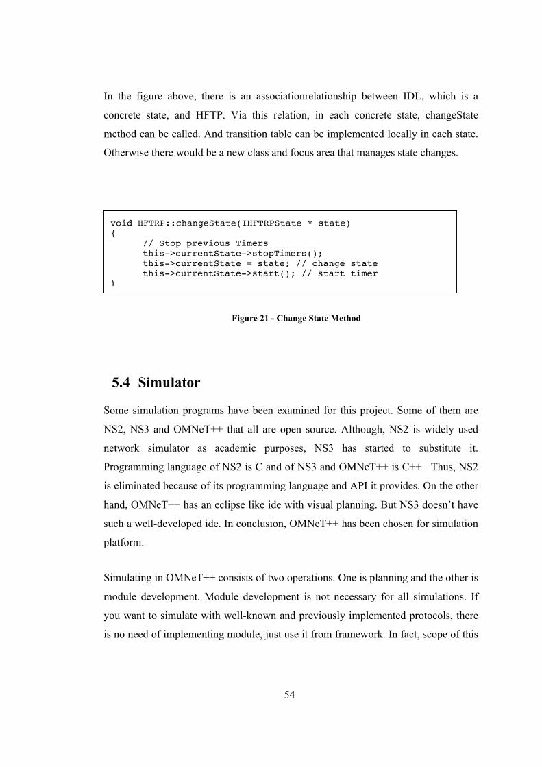
54

In the figure above, there is an associationrelationship between IDL, which is a

concrete state, and HFTP. Via this relation, in each concrete state, changeState

method can be called. And transition table can be implemented locally in each state.

Otherwise there would be a new class and focus area that manages state changes.

5.4 Simulator

Some simulation programs have been examined for this project. Some of them are

NS2, NS3 and OMNeT++ that all are open source. Although, NS2 is widely used

network simulator as academic purposes, NS3 has started to substitute it.

Programming language of NS2 is C and of NS3 and OMNeT++ is C++. Thus, NS2

is eliminated because of its programming language and API it provides. On the other

hand, OMNeT++ has an eclipse like ide with visual planning. But NS3 doesn’t have

such a well-developed ide. In conclusion, OMNeT++ has been chosen for simulation

platform.

Simulating in OMNeT++ consists of two operations. One is planning and the other is

module development. Module development is not necessary for all simulations. If

you want to simulate with well-known and previously implemented protocols, there

is no need of implementing module, just use it from framework. In fact, scope of this

void HFTRP::changeState(IHFTRPState * state) { // Stop previous Timers this->currentState->stopTimers(); this->currentState = state; // change state this->currentState->start(); // start timer }

Figure 21 - Change State Method

55

thesis is a newly developing protocol. Consequently, two modules have been

developed; HFTRP and simple network layer modules.

First, the simulation scenarios have been planned. These scenarios will be explained

at next chapter, test results. But, here the fundamentals will be explained.

Simulation consists of nodes, world and connection manager modules. Connection

manager controls the virtual connections between nodes according to distance and

txpower. World module determines the locations of nodes and boundaries for

mobility actions. Nodes are the main part of simulation. Nodes’ configuration is

simple network layer, nic that consists of mac layer and phy layer, mobility and

utility modules. That is mac layer is HFTRP, which has been developeded.

Figure 22 and Figure 23 shows the graphical representations of these modules.

Figure 22 – Node and Nic Contents

56

Figure 23 - Scenerio Planning Example

57

CHAPTER 6

6. TEST RESULTS

In the scope of this thesis two protocols have been developed. These are original

HFTRP and Improved HFTRP. These two protocols are compared according to some

performance criteria. In this chapter, scenarios and results of these comparisons will

be explained. What are the performance enhancements for Improved-HFTRP will be

analyzed.

6.1 Real Environment Tests

In real environment, only three-node tests have been performed, due to the lack of

physical equipments. Because, radios and modems for HF are too expensive. This

test setup contains three ships that are equipped with HF Modems and HF Radios.

Thus, in real environment only ring creation and growing up to three nodes have

been tested. Related test results are given in the Figure 25 according to the mean

times. Configuration of each node and scenario is given at Figure 24.

Figure 24 - Real Environment Scenario

58

Figure 25 - Real Environment Test Results

Figure 25 shows the test results of real environment with comparison of original

HFTRP and Improved-HFTRP. In this chart, it can be easily seen that, removing one

state and one timer associated with this state makes ring creation with two nodes 35

seconds faster than original HFTRP. Then, in growing scenario, with original

HFTRP growing occurs in 58 seconds and with Improved-HFTRP growing occurs in

31 seconds. Actually, the source of this improvement lies on the proposed values of

scalar tuning parameters. Scalar tuning parameters directly effecting ring growing are

successor number of slots, cycle per solicitation, slot size and successor wait time.

Thus, in real environment with three nodes, performance enhancement on ring

creation and ring growing can be seen. In simulation environment much more tests

have been performed which cannot be easily performed in real environment, due to

lack of equipment and time.

59

6.2 Simulator Tests

Too many tests and scenarios have been done in simulator. However, only limited

number of tests in real environment has been achieved. In simulation environment,

Ring formation, latency, throughput tests and robustness test of ring formation have

been conducted. Results will be discussed on next sections.

6.2.1 Ring Formation

In this test, simulation has been run six times for each scenario. Main characteristic

of each scenario is each node can communicate with all other and no data errors. In

fact each node has powerful radio outputs that can transmit data to all others. On the

other hand this scenario has been run for two configuration; three-node and six-node

configuration. Other configurations of nodes have the same with real environment

tests.

Figure 26 - Simulation Results for 3-node at Ideal Channel

60

Figure 26 shows the test results of simulation with comparison of original HFTRP

and Improved-HFTRP for three nodes.

When the two charts for three nodes are examined, for real environment and

simulation environment, however times are not equal, performance differences are

parallel. Therefore, simulation environment can be used to see performance

enhancements.

Figure 27 - Simulation Results for 6-node at Ideal Channel

Figure 27 shows the test results of simulation with comparison of original HFTRP

and Improved-HFTRP for six nodes.

When two charts for simulation environment are compared, it can be seen that first

creation of ring and growing to three nodes are happening much earlier at six-node

environment than three-node environment. Main reason of this behavior is that there

are six nodes contending for channel, thus probability of choosing first slot get much

61

higher and when first node transmits the others give up transmitting SLS token.

Instead, they reply with SET here it doesn’t matter if there are collisions. Because,

only one station not colliding is enough to grow the ring. The only possibility of

waste of bandwidth is that all stations choose the same channel.

6.2.2 Latency Tests

As a latency test, periodic data of 200 bytes of data have been generated each 5

seconds. When running this test, the same configuration with previous tests has been

used. Data has been stamped with time when it has been generated. Then, the

stamped time is compared with the real time when transmitting to the channel. In

fact, this method is used to check the waiting time of data on the transmit queue. This

time is important on time critical data, like surveillance data. These tests have been

conducted in four different scenarios; 3 nodes running 1,000 seconds, 6 nodes

running 1,000 seconds, 3 nodes running 10,000 seconds and 6 nodes running 10,000

seconds.

Results are visualized as charts and these charts are given in Figure 28 and Figure 29

and interpretations according to min, max and mean values of these charts are given

on the following paragraphs.

Table 16 - Latency values for 3 nodes for 1000 sec

Original HFTRP Improved HFTRP

Min Max Mean Min Max Mean

Ship 1 0.1 72.5 11.2 0.06 26.4 4.8

Ship 2 0.02 111.2 15.5 0.07 14.8 4.1

Ship 3 0.02 66.2 10.5 0.1 25.6 4.9

62

Figure 28 - Packet Latency on 3 nodes for 1000s

Charts at Figure 28 are for packet latencies on 3-node network for 1000 s. First chart

is for Original HFTRP and the second one for Improved-HFTRP. As seen from the

charts maximum packet latency at Improved-HFTRP is smaller than original one.

This is because ring creation is faster in Improved-HFTRP than the original HFTRP.

After ring creation, at each protocol packet latencies get stabile. Still, Improved-

HFTRP has smaller values. Table 16 shows the numeric values for each ship and

network.

Charts at Figure 29 are for packet latencies on 6-node network for 1000 s. First chart

is for Original HFTRP and the second one for Improved-HFTRP. As seen from the

charts maximum packet latency at Improved-HFTRP is smaller than original one.

This is because ring creation is faster in Improved-HFTRP than the original HFTRP.

After ring creation in each protocol packet latencies get stabile and again Improved-

HFTRP has smaller values. And also some rises can be seen on original HFTRP,

these rises are occurring because of long solicitation waitings. Table 17 shows

numerical values for each ship on original HFTRP and Improved-HFTRP.

63

Figure 29 - Packet Latency on 6 nodes for 1000s

Table 17 - Latency values for 6 nodes for 1000 sec

Original HFTRP Improved HFTRP

Min Max Mean Min Max Mean

Ship 1 0.2 315 72.6 4.07 248.1 65.3

Ship 2 0.2 480 134 1.01 103.9 33.4

Ship 3 0.2 65.7 21 3.9 300.8 80.1

Ship 4 0.1 78.8 24.6 0.1 128.1 35.5

Ship 5 0.3 198.4 44.2 0.8 174.5 39.2

Ship 6 0.3 113.5 26.7 0.2 102.4 30.8

Four charts in Figure 30 and Figure 31 are for packet latencies on 3-node and 6-node

network for 10000 s. Charts on first column are for Original HFTRP and on the

second column for Improved-HFTRP. As seen from the charts maximum packet

latency at Improved-HFTRP is smaller than original ones. This is because ring

creation is faster in Improved-HFTRP than original HFTRP. After ring creation in

each protocol packet latencies get stabile and again Improved-HFTRP has smaller

64

values. Because, solicitations in original HFTRP occurs more frequent than

improved-HFTRP and reply waiting time for solicitation period in original HFTRP is

more than improved-HFTRP. Also mean values seem small in Original HFTRP.

However, at Original HFTP mean values varies in a large scale. At Improved HFTRP

mean values are in small scale.

Figure 30 - Packet Latency on 3-node for 10000 sec

Figure 31 - Packet Latency on 6-node for 10000 sec

65

Figure 32 - Packet Latency on 3 nodes after ring formation

Figure 33 - Packet latency on 6 nodes after ring formation

Figure 32 and Figure 33 shows packet latencies for 3 and 6 nodes relatively, where

packet generation started just after ring formation. Firstly, it can be easily seen that

At Improved HFTRP packet latencies are much more smaller than the original

HFTRP. Secondly, when two latencies compared for 3 nodes and 6 nodes, it can be

66

seen that packet latencies for 6 nodes gets more than twice of latencies for 3 nodes.

Main reason of this behavior is at 3-node network token comes after 2 nodes but in

6-node network token comes after 5 nodes, hence latency gets more than twice.

To sum up the latency section, packet latencies on Improved HFTRP are smaller than

original HFTRP. Because, waiting time in solicitation is less at Improved HFTRP

than Original HFTRP. Moreover, number of solicitations is less in Improved

HFTRP. Thus, time wasted for solicitation is much less at improved HFTRP than

original HFTRP. Secondly, when number of nodes gets twice, latencies gets more

than twice, due to the token pass times. At 6-node network token round times are

much more than at 3-node network. In three-node network RTT token rounds again

to the ring owner just after two nodes, which means two token transmitting times

used as overhead in each cycle. However, in six-node network RTT token rounds

again to the ring owner after five nodes, which means five token transmitting times

used as overhead in each cycle.

6.2.3 Throughput Tests

While running this test, configurations of nodes were kept the same with other tests.

As a throughput test, when the nodes first started, application generated 200 bytes of

data that can be send maximum theoretically in the speed of channel which is 2400

bps for our configuration. In other words, the theoretical throughput for 2400 bps is

300 bytes for 1 second, 300 KB for 1000 seconds and 3000 KB for 10000 seconds.

Results and comparison is given at Table 18.

From the Table 18, although, it can be easily seen that, with small data overhead gets

higher and with large data overhead gets too small, in the nature of HF

communication small data has been transmitted instead of large amount. By the way,

ring cannot grow up to three nodes with original HFTRP in 1000 seconds. Thus, at

least 1000 seconds, in other words 16 minute, should be waited before the last node

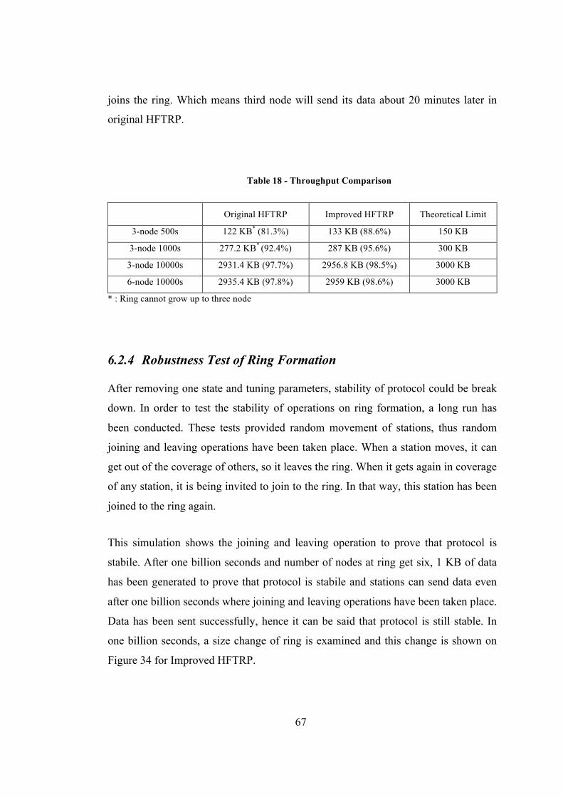
67

joins the ring. Which means third node will send its data about 20 minutes later in

original HFTRP.

Table 18 - Throughput Comparison

Original HFTRP Improved HFTRP Theoretical Limit

3-node 500s 122 KB* (81.3%) 133 KB (88.6%) 150 KB

3-node 1000s 277.2 KB* (92.4%) 287 KB (95.6%) 300 KB

3-node 10000s 2931.4 KB (97.7%) 2956.8 KB (98.5%) 3000 KB

6-node 10000s 2935.4 KB (97.8%) 2959 KB (98.6%) 3000 KB

* : Ring cannot grow up to three node

6.2.4 Robustness Test of Ring Formation

After removing one state and tuning parameters, stability of protocol could be break

down. In order to test the stability of operations on ring formation, a long run has

been conducted. These tests provided random movement of stations, thus random

joining and leaving operations have been taken place. When a station moves, it can

get out of the coverage of others, so it leaves the ring. When it gets again in coverage

of any station, it is being invited to join to the ring. In that way, this station has been

joined to the ring again.

This simulation shows the joining and leaving operation to prove that protocol is

stabile. After one billion seconds and number of nodes at ring get six, 1 KB of data

has been generated to prove that protocol is stabile and stations can send data even

after one billion seconds where joining and leaving operations have been taken place.

Data has been sent successfully, hence it can be said that protocol is still stable. In

one billion seconds, a size change of ring is examined and this change is shown on

Figure 34 for Improved HFTRP.

68

Figure 34 - Change of ring size in one billion seconds of time period

Figure 34 shows the change of ring size from the view of one station in one billion

seconds, which is more than eleven days. Firstly, it can bee seen that, this station has

been joined to the ring as fifth node. Then one another station joined to the rind and

ring size got six. After awhile, nodes at ring went to two and than again six one by

one. Furthermore, it can be seen that from three hundred thousand to six hundred

thousand all nodes are in the ring. Finally, it can be seen that four times this station

left the ring. This can be understood from ring size where is one.

As a conclusion, Improved HFTRP performed all joining and leaving operations

healthy and at the end sent 1 KB of data from each station successfully. Thus,

Improved HFTRP can be used instead of Original HFTRP.

69

CHAPTER 7

7. CONCLUSION

Main aim of this thesis is to improve ring creation and growing capabilities. In other

words, ring creation and growing was a slow operation and it should have been get

faster. Here in this thesis improvement methods have been discussed and test results

collected for both original and with proposed improvements. In fact, results showed

that proposed improvements enhanced ring formation procedure. For example, ring

formation in a 3-node environment was 139 seconds as average, however with

proposed improvements it reduced to the level of 77 seconds at real environment.

Moreover, it was 100 seconds for original HFTRP and get to 65 second average in

simulation environment. In other words, the gain is nearly 40% in average of tests.

The 6-node environment tests have been performed on simulation environment.

Results were also dramatic. That are, total time to form a 6-node ring was 220

seconds with original HFTRP and with Improved-HFTRP it gets to 121 seconds for

mean of tests. In other words, this means 45% of gain. However, these tests are done

without data, tests with data also has enhancements but not at the same level.

At tests with data we measured packet latency and throughput. For packet latency it

can be said that for periodic data Improved-HFTRP is much more efficient when

sending data starts with the node starts. However, in throughput, for small data

Improved-HFTRP has advantages, for large data nearly there are no improvements.

Because, Improved-HFTRP aims to improve ring setup and growing and when ring

gets stabile, these operations will take place in the same way with original HFTRP.

Therefore, 100 seconds of 10000 seconds as improvement will not affect much the

overall performance.

70

To sum up, if our clients generally generate periodic data, such GPS data, and small

data like chat or small files, using Improved-HFTRP gives much more gain.

However, if clients generally generate large amount of data, then the Improved-

HFTRP will not contribute much to the overall performance. In fact, in HF medium

mostly small data as GPS, surveillance, chat and messaging, etc is being generated,

thus Improved-HFTRP would give significant performance improvements.

As a future work, relaying operation in HFTRP can be enhanced. However, it is just

limited with relaying of RTT token as REL token. As a future work in this area, relay

operations with data capability can be added to protocol and these operations can be

combined with routing. Moreover, REL token can be substituted by RTT token. In

other words, REL token uses NS field as a final target, however, in RTT token this

field is unused. Thus, RTT token can be changed to use NS field for relaying.

71

REFERENCES

[1] A.S. Tanenbaum, Computer Networks, Prentice-Hall, 2002. [2] Buddenberg,R., HF Capacity, http://web1.nps.navy.mil/~budden/lecture.notes/r-wan/hf.html, last accessed

on 03/12/2010. [3] Ergen,M, WTRP – Wireless Token Ring Protocol, University of California,

Berkeley, Spring 2002. [4] Harris Assured Communications, Radio Communications in the Digital Age,

Harris Corporation 2005. [5] Gamma,E., Helm,R., Johnson,R. and Vlissides,J., Design Patterns: Elements

of Reusable Object-Oriented Software, Addison Wesley, pp ,144-154,338-348, November 10,1994.

[6] Goldshmit, A., Wireless Communications, Cambridge University Press, p

268, 2005. [7] Johnson,E.E., et al., Advanced High-Frequency Radio Communications,

Artech House, 1997. [8] Johnson,E.E., et al, Robust Token Management For Unreliable Networks,

Proceedings of MILCOM 2003, Boston, MA, 2003 [9] Johnson, E.E., Balakrishnan, M. and Tang,Z., Impact Of Turnaround Time

On Wireless MAC Protocols, Proceedings of MILCOM 2003, Boston, MA, 2003.

[10] Johnson, E.E., Tang, Z. and Balakrishnan, M., Token relay with optimistic

joining, Military Communications Conference, 2005. MILCOM 2005. IEEE, pp.2216-2222 vol. 4, 17-20 Oct. 2005.

[11] IEEE 802.5, Token ring access method and Physical Layer specifications,

IEEE Computer Society, 1998. [12] NC3A, NATO Standardization Agreement: Profile for High Frequency (HF)

Radio Data Communications, STANAG 5066, Edition 2, Promulgated on 5 December 2008.

[13] NC3A, NATO Standardization Agreement: Profile for High Frequency (HF)

Radio Data Communications, STANAG 5066, Edition 2 Draft 2,NATO,2008.

72

[14] Nyquist, H., Certain Factors Affecting Telegraph Speed, Bell System

Technical Journal, pp. 324, April 1924. [15] OMNeT++ Home Page http://www.omnetpp.org/, last accessed on 03/12/2010 [16] Reynolds, A.B., Blair, W.D., Tactical High Frequency Communications in

the Land Arena - The Current State of the Art, DSTO, September 2001. [17] Shannon,C.E., A Mathematical Theory of Communication, The Bell System

Technical Journal vol 27, pp 379, USA, July, October 1949. [18] Wikipedia contributors, Interleaver, Wikipedia,

http://en.wikipedia.org/wiki/Interleaver, last accessed on 27/12/2010