Improved Inputs Use and Productivity in Uganda's Maize Sub-sector

RESEARCH SERIES No. 69

IMPROVED INPUTS USE AND PRODUCTIVITY IN

UGANDA’S MAIZE SUB‐SECTOR

By

GEOFREY OKOBOI

ECONOMIC POLICY RESEARCH CENTRE

MARCH 2010

ABSTRACT

This paper used the Uganda National Household Survey (UNHS) dataset of 2005/06 to examine the productivity of improved inputs used by smallholder maize farmers in Uganda. Yield and gross profit functions were estimated with the stochastic frontier model. Results revealed a significant effect improved inputs use on yield but not gross profit. Moreover, farmers who planted recycled seed (of improved variety) without fertiliser obtained lower yield but the highest gross profit. Furthermore, if the opportunity cost of own land and labour inputs in maize production were imputed, overall, farmers made economic losses. Based on the prevailing farmers’ production technology and market conditions, maize cultivation in the range of 2‐3 ha was found to give optimum profit while cultivation under 1 ha or above 4 ha led to economic losses. A major contribution of this paper is that maize cultivation in Uganda in 2005/06 and even at present was/may be of no economic consequence other than food, at household level.

E c o n o m i c p o l i c y R e s e a r c h C e n t r e | M a r c h 2 0 1 0 Page i

E c o n o m i c p o l i c y R e s e a r c h C e n t r e | M a r c h 2 0 1 0 Page ii

Table of Contents

ABSTRACT ......................................................................................................................................... I

1.0 INTRODUCTION .................................................................................................................. 1

3.0 REVIEW OF RELATED LITERATURE ...................................................................................... 6

4.0 DATA AND METHODS ....................................................................................................... 10

4.1 Data ......................................................................................................................... 10

4.2 Method of analysis .................................................................................................. 13

5.0 RESULTS AND DISCUSSION ............................................................................................... 15

5.1 Yield and labour productivity ................................................................................... 15

5.2 Distribution of yield and gross profit ....................................................................... 16

5.3 Comparison of yield and gross profit against seed type and fertiliser use .............. 17

5.4 Costs and returns in maize production .................................................................... 19

5.5 Econometric results.................................................................................................. 21

6.0 CONCLUSIONS AND IMPLICATIONS .................................................................................. 27

REFERENCES .................................................................................................................................. 29

List of Tables

TABLE 1: VARIABLES OF THE STUDY, THEIR UNITS OF MEASUREMENT AND DESCRIPTIVE STATISTICS. ............. 11

TABLE 2: YIELD AND LABOUR PRODUCTIVITY .......................................................................................... 15

TABLE 3: COMPARISON OF LABOUR PRODUCTIVITY AND LABOUR WAGE .................................................... 16

TABLE 4: DISTRIBUTION OF YIELD AND GROSS PROFIT ............................................................................. 17

TABLE 5: AVERAGE EXPENDITURE AND RETURNS PER HECTARE OF MAIZE, UGX MILLIONS ........................... 20

TABLE 6: MAXIMUM LIKELIHOOD ESTIMATES OF THE YIELD AND GROSS PROFIT –HALF NORMAL MODEL ....... 22

List of Figures

Figure 1: Area cultivated, output and yield of Maize in Uganda ..................................................... 4

Figure 1: Yield and gross profit comparison by seed type with and without fertiliser use ........... 18

Figure 3: Estimated costs and returns based on area cultivated .................................................. 21

1.0 INTRODUCTION

By any measure, Uganda is an agricultural country. Despite the declining contribution of

agriculture to overall Gross Domestic Product (GDP) –now estimated at 15.1 percent,

the sector remains the main source of livelihood to nearly 73 percent of the Uganda’s

labour force (Uganda Bureau of Statistics ‐ UBoS, 2006). The bulk of Uganda’s exports

are agricultural commodities and much of the industrial activity is in agro‐processing.

Growth of agriculture is critical to the growth of the overall economy and poverty

reduction in Uganda (Sennoga and Matovu, 2010). However, despite the fact that rapid

growth in agriculture is important for Uganda, it remains dismal –averaging 1.3 per cent

over the past 5 years (MFPED, 2009).

Countries –particularly in Asia that have registered consistently high grow rates in

agriculture have also been associated with sizeable increases in the use of improved

production technologies compared to other inputs including land or labour (Hazell and

Rosegrant, 2000). Increases in per capita use of fertiliser, high yielding seed varieties,

traction power and irrigation are particularly commended for the Asian green revolution

(World Bank, 2007).

In the case of Uganda, however, use of improved agricultural technologies remains low

(UBoS, 2007), even when most farmers may be aware of the potential of these inputs to

increase yield. But yield per se may not be enough to guarantee increased adoption ‐

especially for poor farmers when the cost of these inputs compared to the farmers’

basic needs may be relatively high. The economic returns from use of these inputs are of

essence than yield (FAO, 2006).

This paper therefore sought to examine the contribution of improved inputs use to

farmer yield and profit in Uganda’s maize sub‐sector. To this end, the overall objective

of this paper was to examine the economic as compared with the physical productivity

of improved inputs use in smallholder maize production. The specific objectives were:

E c o n o m i c p o l i c y R e s e a r c h C e n t r e | M a r c h 2 0 1 0 Page 1

(i) To compare the yield and profit of smallholder farmers under various input‐

mix production practices;

(ii) To examine the contribution of each improved input to productivity, and

(iii) To examine the relationship between farmer attributes and productivity.

By concurrently analysing the impact of improved inputs use on the physical and

economic productivity, this will shade light on the less‐often asked but important

question of why farmers are not using improved technologies in Uganda as would be

expected. Certainly, a better understanding of the farmer’s physical as compared to

economic productivity from their diverse input‐mix production practices is key to

appropriate policy intervention. Also, given the fact that the revised 5‐year (2010/11‐

2014/15) Development Strategy and Investment Plan (DSIP) of Ministry of Agriculture

Animal Industry and Fisheries (MAAIF) (MAAIF, 2010) is focussing on investing in the

maize sub‐sector as one of the 10 strategic crops, results of this paper should be of

interest to policy‐makers.

The remainder of the paper is organised into 4 sections. A brief overview of Uganda’s

maize sub‐sector is presented in the next section, which is followed by the review of

literature. Section 4 describes the data and the method of analysis. Empirical results and

discussion is given in Section 5 while the conclusion and implications of the study are

given in the last section.



2.0 OVERVIEW OF UGANDA’S MAIZE SUB‐SECTOR

Maize is a very important crop in Uganda. It is the most highly cultivated crop. Statistics

from the Uganda National Household Survey (UNHS) of 2005/06 show that maize was

cultivated on an estimated area of 1.54 million hectares (ha) by about 86 percent of the

4.2 million agricultural households (Uganda Bureau of Statistics (UBoS), 2007). Maize is

the number one staple for the urban poor, in institutions such as schools, hospitals and

the military. Also, the crop is the number one source of income for most farmers in

eastern, northern and north‐western Uganda (Ferris et al, 2006).

Other than food, maize has had a wide range of other uses including processing of

livestock and poultry feeds and making of local brew. All this has made maize is the

most traded food‐crop in Uganda. Maize grain was the first food crop to be traded

under the Uganda warehouse receipt system (WRS) since the inception of WRS services

in 2006 (Rural Savings Promotion and Enhancement of Enterprise Development –SPEED,

2006)1. Besides, in the same year of 2006, maize topped the list of food exports, earning

the country over $24 millions2.

Although there are many other industrial formulations that can be developed from

maize, this component of the value‐chain is not yet fully exploited in Uganda’s maize

sub‐sector. For example, maize is used in the manufacture of cooking oil, ethanol which

is an additive in gasoline (bio‐fuel), starch and syrup –which are used in the manufacture

of medicines.

Because of the multiplicity of uses, maize is highly regarded as a strategic food security

crop in Uganda. This is even outlined in the revised DISP (MAAIF, 2010). Maize is the

only cereal crop selected as part the 10 priority crops government is to support under

the revised DSIP. The planned government intervention in the maize sub‐sector is in the

1 Though other crops traded under the Uganda WRS are paddy rice, coffee and cotton, maize remains the dominant and most successful traded commodity. 2 http://www.ugandaexportsonline.com/docs08/statistics/export_stats_2002‐06.pdf

http://www.ugandaexportsonline.com/docs08/statistics/export_stats_2002-06.pdf


area of seed multiplication and distribution, extension services provision, establishment

of warehouses, and research.

However, like other food crops, maize cultivation in Uganda is on smallholder farms –

characterised by low and sometimes declining productivity. According to 2005/06 UNHS

report, between 1999/2000 2005/06, the number of plots under maize have increased

over five‐fold from 1539 to 8422 million, but average plot size has declined. Decline in

area cultivated has been blamed on the increasing agricultural households yet farmland

remains relatively fixed. Production statistics from the Food and Agricultural

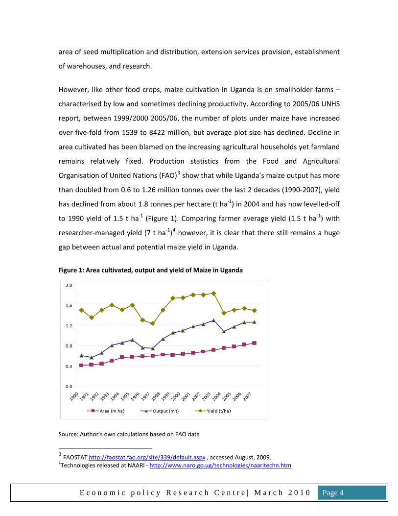
Organisation of United Nations (FAO)3 show that while Uganda’s maize output has more

than doubled from 0.6 to 1.26 million tonnes over the last 2 decades (1990‐2007), yield

has declined from about 1.8 tonnes per hectare (t ha‐1) in 2004 and has now levelled‐off

to 1990 yield of 1.5 t ha‐1 (Figure 1). Comparing farmer average yield (1.5 t ha‐1) with

researcher‐managed yield (7 t ha‐1)4 however, it is clear that there still remains a huge

gap between actual and potential maize yield in Uganda.

Figure 1: Area cultivated, output and yield of Maize in Uganda

0.0

0.4

0.8

1.2

1.6

2.0

1990

1991

1992

1993

1994

1995

1996

1997

1998

1999

2000

2001

2002

2003

2004

2005

2006

2007

Area (m ha) Output (m t) Yield (t/ha)

Source: Author’s own calculations based on FAO data

3 FAOSTAT http://faostat.fao.org/site/339/default.aspx , accessed August, 2009. 4Technologies released at NAARI ‐ http://www.naro.go.ug/technologies/naaritechn.htm

http://faostat.fao.org/site/339/default.aspx

http://www.naro.go.ug/technologies/naaritechn.htm


Limited use of improved inputs including improved seed, fertilisers, herbicides/

fungicides and traction power in production by farmers, is widely regarded as the major

constraint to agricultural productivity growth in Uganda (Ministry of Finance Planning

and Economic Development (MFPED), 2008; MAAIF, 2010). Statistics from UBoS (2007)

show that just 6, 1 and 3 percent of farming parcels planted with crops in Uganda used

improved seed, fertilisers, and herbicides/ fungicides respectively in production. Beside

low use, the quality of inputs on the market is in many instances is tampered with5,

which also greatly affect productivity. Other than low use and tampered quality,

however, inefficient use of improved inputs such as fertilisers by farmers in Uganda is

not uncommon.

5 See www.monitor.co.ug, “NAADS seeds fail to germinate”, Jul 14, 2008 by James Eriku

http://www.monitor.co.ug/

3.0 REVIEW OF RELATED LITERATURE

Inquiry into the contribution of agricultural inputs (including the quality of inputs) to

output variation or factor productivity and total factor productivity in cross section or

over time continues to attract research interest, though it is not new. Heady (1946) as

quoted in Mundlak (2001) pioneered work in agricultural productivity analysis by

estimating the Cobb and Douglas function on farm‐level data. In the analysis, Heady

(1946) calculated the elasticities of land, labour and other assets and variable inputs

(read improved inputs) in production. Besides quantity, the quality of the inputs as well

as farm management were regarded as important factors in production variation –but

were never included due to lack of appropriate data, Mundlak (2001).

Since then, there has been an upsurge of studies on agricultural productivity, be it at

farm or aggregate level; national or cross‐country; and cross‐sectional or longitudinal.

Most of these studies however have focussed on physical productivity (yield) in isolation

of the economic productivity. Yet the economic productivity of the input –as indicated

by the value to cost ratio, is one of the most important determinants of its adoption

(FAO, 2006). Moreover, studies that have concurrently analysed the contribution of

factor inputs to physical and economic productivity (for example, Bravo‐Ureta and

Pinheiro, 1997) show that in most of the cases, there is a marked difference.

The method of analysis of agricultural productivity has to a great extent evolved from

the predominantly Cobb‐Douglas production function estimation approach to other

methods such as the translog function (for example, Ray, 1982; Hyuha et al., 2007), the

quadratic function (Shumway et al., 1988; Huffman and Evenson, 1989), the data

envelop analysis (Chavas and Cox, 1988; Tauer, 1995; Coelli and Rao, 2003), and the

stochastic frontier analysis (SFA) (for example, Ali and Flinn, 1989; Kolawole, 2006;

Oladeebo and Fajuyigbe, 2007). Of all the methods, the SFA has however gained more

prominence in recent years.


Concerning the impact of improved inputs on productivity, most studies are unanimous

of the positive and significant impact of fertiliser on yield (World Bank, 2007). But

results of the economic returns of fertiliser remain mixed. For example, Kelly and

Murekezi (2000) found that fertiliser use in most areas of Rwanda was profitable for

some crops (such as maize and potatoes) but not for others –for example, sorghum and

beans. In the case of seed, the World Bank (2007) provides extensive literature of the

positive impact of improved seeds varieties on yield in Asia and even in Sub‐Saharan

Africa, but little is said on the economic returns from using these seeds especially for

smallholder farmers in Africa.

The influence of farmer characteristics and farm attributes on productivity has received

great attention in productivity analysis. For example, studies including Owens et al.

(2003), Evenson and Mwabu (1998), Bravo‐Ureta and Evenson (1994), Kalirajan (1991)

report a positive and significant relationship between farm‐level yield and access to

extension services. In the case of education level, results are mixed. Some studies report

a positive and significant relationship between education level and yield –for example

Evenson and Mwabu (1998), others report an inverse relation (Aguilar, 1988) and yet

other studies have reported no statistical significance (Bravo‐Ureta and Evenson, 1994).

The issue of gender in productivity has received a fair share of research attention. A

study of gender efficiency in agricultural production by Udry (1994) in Burkina Faso

found that that plots controlled by women had notably lower yields than similar plots

controlled by men within the same household planted with the same crop in the same

year. Udry however noted that yield differentials were due to allocative, rather than

technical inefficiency of women managed farms given the significantly higher labour and

fertiliser inputs per acre on plots controlled by men. Saito et al (1994) also reported a

positive although insignificant coefficient of gender (male plot manager) effect on yield

in a study in Kenya.


The effect of weather on farmer yield has been analysed by Akpalu et al. (2008). Using

precipitation and temperature data, the authors found that a unit increase in the mean

precipitation had a considerably favourable impact on yield while a decrease in

precipitation had a negative impact on the yield of maize farmers in South Africa.

Rahman (2003) used a stochastic profit frontier function to model the profit inefficiency

effects that may arise from farmer characteristics and access to extension and

infrastructure services among other factors. Results of his study indicated that soil

fertility, access to extension and farmer experience were positively associated with

increased profit efficiency. Using farm‐level survey data and SFA approach, Kolawole

(2006) also reported that age, farmer experience, education level, and household size

positively affected the profit efficiency of small scale rice farmers in Nigeria.

Analysis of agricultural productivity in Uganda has attracted a reasonable number of

studies, most especially in the area of land productivity. Using the Uganda Integrated

Household survey data of 1992/3 and 1993/94, Deininger and Okidi (2001) show that

increase in value of farmers’ output was positively associated with the value of land,

labour and fertiliser used in production. Years of experience and the level of education

were also found to play a positive role in increasing household output. In an earlier

study, Appelton and Balihuta (1996) had also found a positive relationship between

education level and household agricultural output. Okello and Laker‐Ojok (2005) found

that farmer productivity was significantly influenced by land topography, level of

rainfall, incidence of pests and diseases, and infrastructural developments. Other factors

found to significantly affect farmer productivity included the level or value of

investment in agricultural production inputs. Hyuha et al. (2007) is one the few studies

that analysed farmer productivity from the profit viewpoint. The study was however

limited to just 3 rice growing districts of Tororo, Pallisa and Lira in eastern and northern

Uganda. In all these studies cited, however, none appears to have simultaneously

considered the impact of improved inputs use on physical and economic productivity.


Studies that have comparatively analysed the impact of improved inputs use on both

yield and profit are scanty in general and virtually absent in the case of Uganda. In the

analysis of either physical or economic productivity, the SFA method has gained

prominence due to its ability to concurrently estimate the significance of both the

stochastic noise and the inefficiency of farm/farmer attributes in productivity. This

paper adopts the SFA modelling approach to examine the relationship between the level

of farmer expenditure on improved inputs and yield and profit in maize farming in

Uganda.



4.0 DATA AND METHODS

4.1 Data

This paper utilized the Uganda National Household Survey (UNHS) data set of 2005/06

collected by the Uganda Bureau of Statistics (UBoS). This dataset is national in scope. It

was collected at household and community level for two seasons and on five modules,

namely: agriculture, socioeconomic, community, price, and qualitative modules.

Agriculture, which was the core module, covered household crop and non‐crop farming

enterprises. On crop enterprises, enquiries were made for example on area under

crop(s), quantity and value of labour inputs, output and sales, value and attributes of

non‐labour inputs. The non‐crop section covered livestock and poultry production and

deposition. The socio‐economic module included farmer characteristics such as location,

age, gender, education level, access to extension services, and access to credit. The

Price module mainly covered market prices for agricultural inputs and outputs.

For this paper, data pertaining to maize production and relevant to the objectives were

filtered from the 5 modules and then merged using unique identifiers. A total of 1888

farm (parcel) observations, distributed by region as in Table 1 were derived.


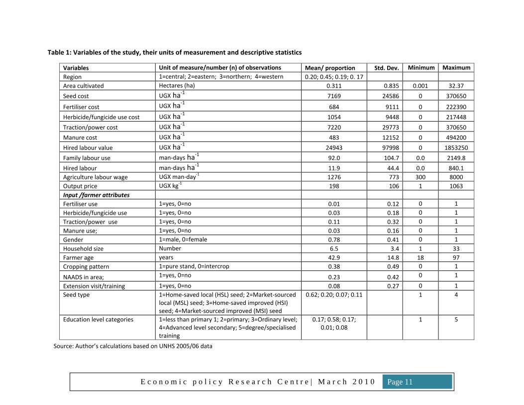
Table 1: Variables of the study, their units of measurement and descriptive statistics

Variables Unit of measure/number (n) of observations Mean/ proportion Std. Dev. Minimum Maximum Region 1=central; 2=eastern; 3=northern; 4=western 0.20; 0.45; 0.19; 0. 17 Area cultivated Hectares (ha) 0.311 0.835 0.001 32.37 Seed cost UGX ha‐1 7169 24586 0 370650

Fertiliser cost UGX ha‐1 684 9111 0 222390 Herbicide/fungicide use cost UGX ha‐1 1054 9448 0 217448 Traction/power cost UGX ha‐1 7220 29773 0 370650 Manure cost UGX ha‐1 483 12152 0 494200 Hired labour value UGX ha‐1 24943 97998 0 1853250 Family labour use man‐days ha‐1 92.0 104.7 0.0 2149.8 Hired labour man‐days ha‐1 11.9 44.4 0.0 840.1 Agriculture labour wage UGX man‐day‐1 1276 773 300 8000 Output price UGX kg‐1 198 106 1 1063 Input /farmer attributes Fertiliser use 1=yes, 0=no 0.01 0.12 0 1Herbicide/fungicide use 1=yes, 0=no 0.03 0.18 0 1Traction/power use 1=yes, 0=no 0.11 0.32 0 1Manure use; 1=yes, 0=no 0.03 0.16 0 1Gender 1=male, 0=female 0.78 0.41 0 1Household size Number 6.5 3.4 1 33 Farmer age years 42.9 14.8 18 97 Cropping pattern 1=pure stand, 0=intercrop 0.38 0.49 0 1

NAADS in area; 1=yes, 0=no 0.23 0.42 0 1

Extension visit/training 1=yes, 0=no 0.08 0.27 0 1Seed type

1=Home‐saved local (HSL) seed; 2=Market‐sourced local (MSL) seed; 3=Home‐saved improved (HSI) seed; 4=Market‐sourced improved (MSI) seed

0.62; 0.20; 0.07; 0.11 1 4

Education level categories

1=less than primary 1; 2=primary; 3=Ordinary level; 4=Advanced level secondary; 5=degree/specialised training

0.17; 0.58; 0.17; 0.01; 0.08

1 5

Source: Author’s calculations based on UNHS 2005/06 data

The units of measurement and the descriptive statistics of mean, standard deviation,

minimum and maximum value of the variables are also given in Table 1. The descriptive

statistics reveal that average area cultivated with maize was 0.31 ha with the highest

area cultivated being 32.4 ha. Farmer expenditure on improved inputs that comprise

improved seed, fertiliser, herbicides/fungicides, traction power and manure averaged

UGX 7170, 680, 1050, 7220, and 480 ha‐1 respectively but with a wide variance as

indicated by their standard deviation. Whereas on average farmers spent most on hired

labour (UGX 24943) than all other inputs combined (about UGX 17000), family labour

use (92 man‐days) outstripped hired labour use (11 man‐days) by 8 times. This suggests

that labour in general and family labour in particular was the dominant input in

production.

The proportion of farmers using improved inputs in production is shown in Table 1,

being 1, 3, 11, and 3 percent for fertiliser, herbicides/fungicides, traction power and

manure respectively. The majority of the farmers planted local maize seed (82 percent) ‐

either saved from past production (62 percent) or sourced from the market (20 percent)

while only 11 percent planted improved seed sourced from market.

The demographic characteristics of the farmers indicate that 78 percent of the farm

managers were male, the average age of the farmers was 43 years and the average

household size was 7 persons. The majority of the farmers (58 percent) had primary

education, 17 percent had no formal education while another 17 percent had ordinary

level education. The majority of the farmers inter‐cropped (62 percent) maize with

other crops. Only 8 percent of the farmers received extension training and/or services.


4.2 Method of analysis

To examine the contribution of improved inputs use in farmer productivity, we follow

the approach of Kumbhakar and Lovell (2000) and estimate a stochastic frontier

production model of the Cobb‐Douglas function for yield and gross profit, specified as:

( ) iexAfy jikiiεβ .,,= ; i = 1,…….N, 1

Where iy is yield or gross profit of farmer i; Aki is the area k under cultivation by farmer

i, xji is the cost of input j used in production by farmer i, β is a vector of coefficients to be

estimated. e is the expression for exponential, and εi is the error term, consisting of the

stochastic term, νi and the inefficiency variables –farmer characteristics, ui. That is;

iii uv −=ε . The νi’s are assumed to be normally distributed and independent of ui’s.

While ui’s are non‐negative random variables associated with the (in)efficiency in the

yield/gross profit. Since the data we used was cross‐sectional, a half‐normal distribution

of the inefficiency variables was assumed in order to obtain efficient estimates (Bauer,

1990).

In general, the model in Eq [1] was composed of two parts –the general model f(.) and

the inefficiency model (ε). In the explicit form, Eq [1] was specified as in Eq [2].

⎥⎦

⎤⎢⎣

⎡⎟⎠

⎞⎜⎝

⎛++++= ∑∑

==

9

10

6

210 lnln

kkikji

jjijjii zvXAy ββααα 2

In Eq [2], ln implies natural logarithm, X1i, X2i, ..,X6i are costs of seed, chemical fertiliser,

herbicides/fungicides, hired labour, manure, and traction power, respectively for farmer

i. On the other hand, Z1, Z2, .., Z9 were farmer characteristics including family size,

gender, age, education level and urban/rural location. Other farmer characteristics

included were cropping pattern, season of farming, extension services access, and

farmer being in area where NAADS operated.


Positive values of the inefficiency covariates (Z’s) indicate the contribution of the

variable towards the overall productivity inefficiency. However, if the value of the

inefficiency covariate is negative, the variable brings about efficiency rather than

inefficiency towards the overall yield/ gross profit of the farmer.

The variables included in Eq [2] are those that are normally included in analyses of this

kind, including studies such as Ali and Finn (1989), Bravo‐Ureta and Pinheiro (1997),

Rahman (2003), and Hyuha et al (2007). Estimation of the parameters (α, β, ν) in Eq [2]

was carried out in one‐step using the maximum likelihood estimation technique in the

Frontier models programme of STATA/SE 10.0 SE.


5.0 RESULTS AND DISCUSSION

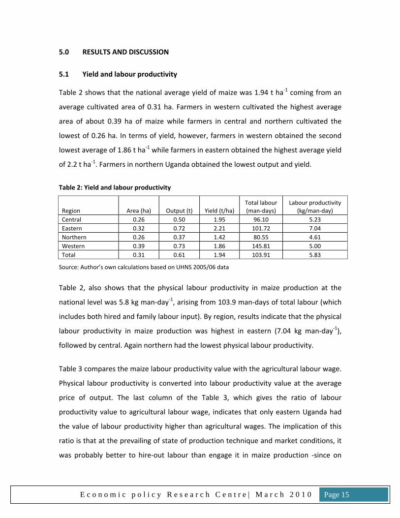
5.1 Yield and labour productivity

Table 2 shows that the national average yield of maize was 1.94 t ha‐1 coming from an

average cultivated area of 0.31 ha. Farmers in western cultivated the highest average

area of about 0.39 ha of maize while farmers in central and northern cultivated the

lowest of 0.26 ha. In terms of yield, however, farmers in western obtained the second

lowest average of 1.86 t ha‐1 while farmers in eastern obtained the highest average yield

of 2.2 t ha‐1. Farmers in northern Uganda obtained the lowest output and yield.

Table 2: Yield and labour productivity

Region Area (ha) Output (t) Yield (t/ha) Total labour (man‐days)

Labour productivity (kg/man‐day)

Central 0.26 0.50 1.95 96.10 5.23 Eastern 0.32 0.72 2.21 101.72 7.04 Northern 0.26 0.37 1.42 80.55 4.61 Western 0.39 0.73 1.86 145.81 5.00 Total 0.31 0.61 1.94 103.91 5.83

Source: Author’s own calculations based on UHNS 2005/06 data

Table 2, also shows that the physical labour productivity in maize production at the

national level was 5.8 kg man‐day‐1, arising from 103.9 man‐days of total labour (which

includes both hired and family labour input). By region, results indicate that the physical

labour productivity in maize production was highest in eastern (7.04 kg man‐day‐1),

followed by central. Again northern had the lowest physical labour productivity.

Table 3 compares the maize labour productivity value with the agricultural labour wage.

Physical labour productivity is converted into labour productivity value at the average

price of output. The last column of the Table 3, which gives the ratio of labour

productivity value to agricultural labour wage, indicates that only eastern Uganda had

the value of labour productivity higher than agricultural wages. The implication of this

ratio is that at the prevailing of state of production technique and market conditions, it

was probably better to hire‐out labour than engage it in maize production ‐since on


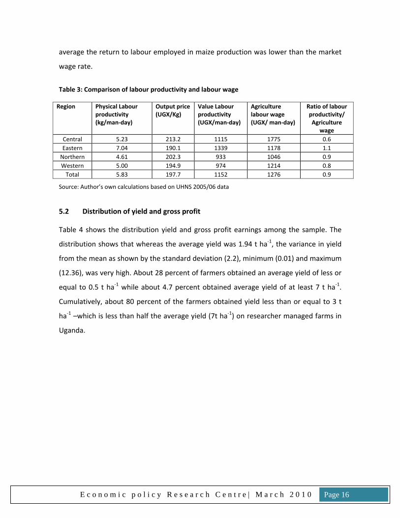
average the return to labour employed in maize production was lower than the market

wage rate.

Table 3: Comparison of labour productivity and labour wage

Region Physical Labour productivity (kg/man‐day)

Output price (UGX/Kg)

Value Labour productivity (UGX/man‐day)

Agriculture labour wage (UGX/ man‐day)

Ratio of labour productivity/ Agriculture

wage Central 5.23 213.2 1115 1775 0.6 Eastern 7.04 190.1 1339 1178 1.1 Northern 4.61 202.3 933 1046 0.9 Western 5.00 194.9 974 1214 0.8 Total 5.83 197.7 1152 1276 0.9


5.2 Distribution of yield and gross profit

Table 4 shows the distribution yield and gross profit earnings among the sample. The

distribution shows that whereas the average yield was 1.94 t ha‐1, the variance in yield

from the mean as shown by the standard deviation (2.2), minimum (0.01) and maximum

(12.36), was very high. About 28 percent of farmers obtained an average yield of less or

equal to 0.5 t ha‐1 while about 4.7 percent obtained average yield of at least 7 t ha‐1.

Cumulatively, about 80 percent of the farmers obtained yield less than or equal to 3 t

ha‐1 –which is less than half the average yield (7t ha‐1) on researcher managed farms in

Uganda.


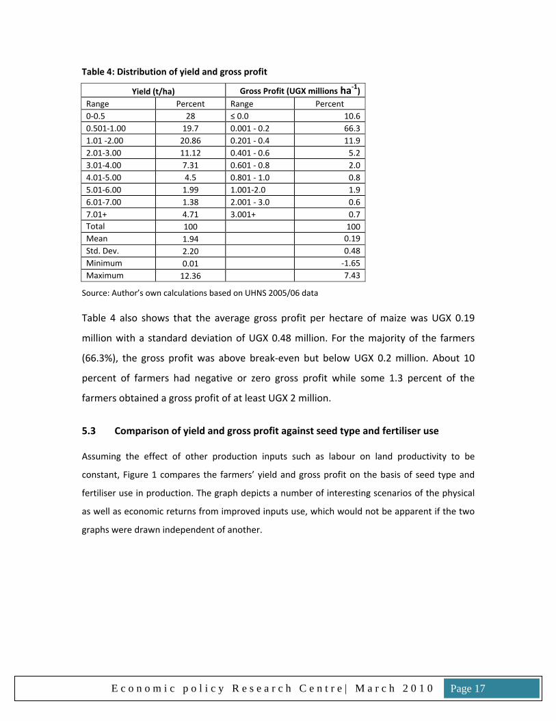
Table 4: Distribution of yield and gross profit

Yield (t/ha) Gross Profit (UGX millions ha‐1) Range Percent Range Percent 0‐0.5 28 ≤ 0.0 10.6 0.501‐1.00 19.7 0.001 ‐ 0.2 66.3 1.01 ‐2.00 20.86 0.201 ‐ 0.4 11.9 2.01‐3.00 11.12 0.401 ‐ 0.6 5.2 3.01‐4.00 7.31 0.601 ‐ 0.8 2.0 4.01‐5.00 4.5 0.801 ‐ 1.0 0.8 5.01‐6.00 1.99 1.001‐2.0 1.9 6.01‐7.00 1.38 2.001 ‐ 3.0 0.6 7.01+ 4.71 3.001+ 0.7 Total 100 100 Mean 1.94 0.19Std. Dev. 2.20 0.48Minimum 0.01 ‐1.65Maximum 12.36 7.43


Table 4 also shows that the average gross profit per hectare of maize was UGX 0.19

million with a standard deviation of UGX 0.48 million. For the majority of the farmers

(66.3%), the gross profit was above break‐even but below UGX 0.2 million. About 10

percent of farmers had negative or zero gross profit while some 1.3 percent of the

farmers obtained a gross profit of at least UGX 2 million.

5.3 Comparison of yield and gross profit against seed type and fertiliser use

Assuming the effect of other production inputs such as labour on land productivity to be

constant, Figure 1 compares the farmers’ yield and gross profit on the basis of seed type and

fertiliser use in production. The graph depicts a number of interesting scenarios of the physical

as well as economic returns from improved inputs use, which would not be apparent if the two

graphs were drawn independent of another.


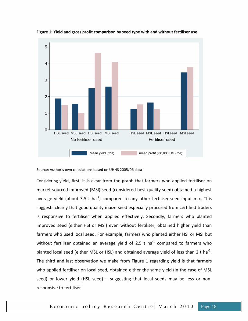
Figure 1: Yield and gross profit comparison by seed type with and without fertiliser use

0

1

2

3

4

5

No fertiliser used Fertiliser usedHSL seed MSL seed HSI seed MSI seed HSL seed MSL seed HSI seed MSI seed

Mean yield (t/ha) mean profit ('00,000 UGX/ha)


Considering yield, first, it is clear from the graph that farmers who applied fertiliser on

market‐sourced improved (MSI) seed (considered best quality seed) obtained a highest

average yield (about 3.5 t ha‐1) compared to any other fertiliser‐seed input mix. This

suggests clearly that good quality maize seed especially procured from certified traders

is responsive to fertiliser when applied effectively. Secondly, farmers who planted

improved seed (either HSI or MSI) even without fertiliser, obtained higher yield than

farmers who used local seed. For example, farmers who planted either HSI or MSI but

without fertiliser obtained an average yield of 2.5 t ha‐1 compared to farmers who

planted local seed (either MSL or HSL) and obtained average yield of less than 2 t ha‐1.

The third and last observation we make from Figure 1 regarding yield is that farmers

who applied fertiliser on local seed, obtained either the same yield (in the case of MSL

seed) or lower yield (HSL seed) – suggesting that local seeds may be less or non‐

responsive to fertiliser.


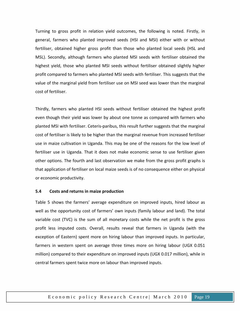
Turning to gross profit in relation yield outcomes, the following is noted. Firstly, in

general, farmers who planted improved seeds (HSI and MSI) either with or without

fertiliser, obtained higher gross profit than those who planted local seeds (HSL and

MSL). Secondly, although farmers who planted MSI seeds with fertiliser obtained the

highest yield, those who planted MSI seeds without fertiliser obtained slightly higher

profit compared to farmers who planted MSI seeds with fertiliser. This suggests that the

value of the marginal yield from fertiliser use on MSI seed was lower than the marginal

cost of fertiliser.

Thirdly, farmers who planted HSI seeds without fertiliser obtained the highest profit

even though their yield was lower by about one tonne as compared with farmers who

planted MSI with fertiliser. Ceteris‐paribus, this result further suggests that the marginal

cost of fertiliser is likely to be higher than the marginal revenue from increased fertiliser

use in maize cultivation in Uganda. This may be one of the reasons for the low level of

fertiliser use in Uganda. That it does not make economic sense to use fertiliser given

other options. The fourth and last observation we make from the gross profit graphs is

that application of fertiliser on local maize seeds is of no consequence either on physical

or economic productivity.

5.4 Costs and returns in maize production

Table 5 shows the farmers’ average expenditure on improved inputs, hired labour as

well as the opportunity cost of farmers’ own inputs (family labour and land). The total

variable cost (TVC) is the sum of all monetary costs while the net profit is the gross

profit less imputed costs. Overall, results reveal that farmers in Uganda (with the

exception of Eastern) spent more on hiring labour than improved inputs. In particular,

farmers in western spent on average three times more on hiring labour (UGX 0.051

million) compared to their expenditure on improved inputs (UGX 0.017 million), while in

central farmers spent twice more on labour than improved inputs.


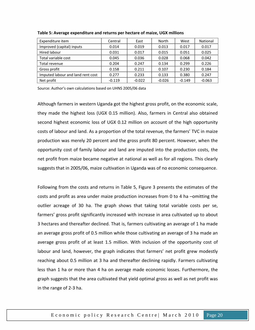
Table 5: Average expenditure and returns per hectare of maize, UGX millions

Expenditure item Central East North West National Improved (capital) inputs 0.014 0.019 0.013 0.017 0.017 Hired labour 0.031 0.017 0.015 0.051 0.025 Total variable cost 0.045 0.036 0.028 0.068 0.042 Total revenue 0.204 0.247 0.134 0.299 0.226 Gross profit 0.158 0.211 0.107 0.230 0.184 Imputed labour and land rent cost 0.277 0.233 0.133 0.380 0.247 Net profit ‐0.119 ‐0.022 ‐0.026 ‐0.149 ‐0.063


Although farmers in western Uganda got the highest gross profit, on the economic scale,

they made the highest loss (UGX 0.15 million). Also, farmers in Central also obtained

second highest economic loss of UGX 0.12 million on account of the high opportunity

costs of labour and land. As a proportion of the total revenue, the farmers’ TVC in maize

production was merely 20 percent and the gross profit 80 percent. However, when the

opportunity cost of family labour and land are imputed into the production costs, the

net profit from maize became negative at national as well as for all regions. This clearly

suggests that in 2005/06, maize cultivation in Uganda was of no economic consequence.

Following from the costs and returns in Table 5, Figure 3 presents the estimates of the

costs and profit as area under maize production increases from 0 to 4 ha –omitting the

outlier acreage of 30 ha. The graph shows that taking total variable costs per se,

farmers’ gross profit significantly increased with increase in area cultivated up to about

3 hectares and thereafter declined. That is, farmers cultivating an average of 1 ha made

an average gross profit of 0.5 million while those cultivating an average of 3 ha made an

average gross profit of at least 1.5 million. With inclusion of the opportunity cost of

labour and land, however, the graph indicates that farmers’ net profit grew modestly

reaching about 0.5 million at 3 ha and thereafter declining rapidly. Farmers cultivating

less than 1 ha or more than 4 ha on average made economic losses. Furthermore, the

graph suggests that the area cultivated that yield optimal gross as well as net profit was

in the range of 2‐3 ha.


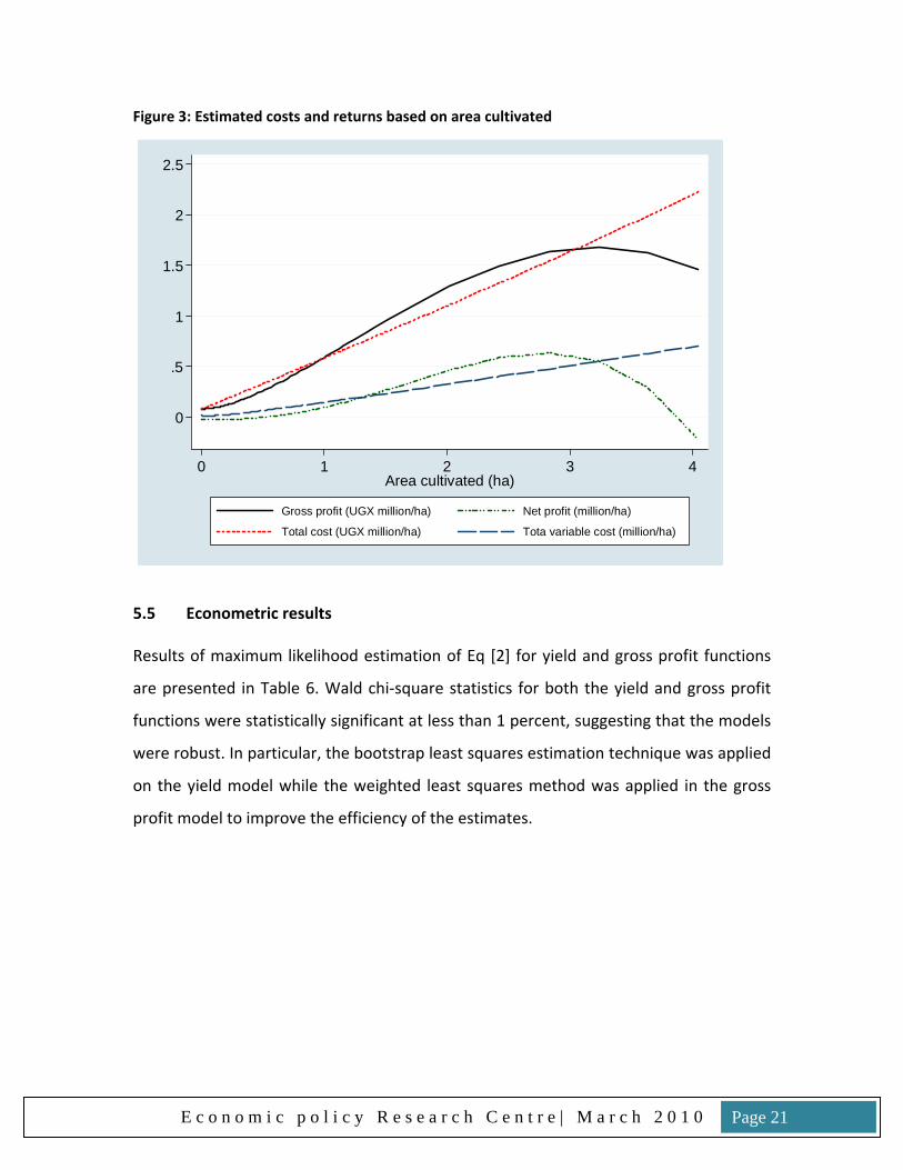
Figure 3: Estimated costs and returns based on area cultivated

0

.5

1

1.5

2

2.5

0 1 2 3 4Area cultivated (ha)

Gross profit (UGX million/ha) Net profit (million/ha)

Total cost (UGX million/ha) Tota variable cost (million/ha)

5.5 Econometric results

Results of maximum likelihood estimation of Eq [2] for yield and gross profit functions

are presented in Table 6. Wald chi‐square statistics for both the yield and gross profit

functions were statistically significant at less than 1 percent, suggesting that the models

were robust. In particular, the bootstrap least squares estimation technique was applied

on the yield model while the weighted least squares method was applied in the gross

profit model to improve the efficiency of the estimates.


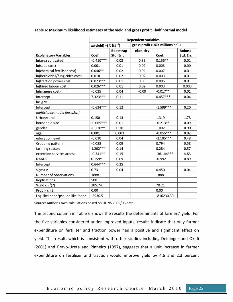
Table 6: Maximum likelihood estimates of the yield and gross profit –half normal model

Explanatory Variables

Dependent variables ln(yield) –( t ha‐1) gross profit (UGX millions ha‐1)

Coef. Bootstrap Std. Err.

elasticityCoef.

Robust Std. Err.

ln(area cultivated) ‐0.410*** 0.03 0.83 0.156** 0.02 ln(seed cost) 0.001 0.01 0.02 0.003 0.00 ln(chemical fertiliser cost) 0.046** 0.02 0.04 0.007 0.01 ln(herbicides/fungicides cost) 0.018 0.02 0.02 0.003 0.01 ln(traction power cost) 0.023*** 0.01 0.03 0.005 0.01 ln(hired labour cost) 0.026*** 0.01 0.02 0.003 0.003 ln(manure cost) ‐0.035 0.04 ‐0.09 ‐0.017** 0.01 Intercept 7.323*** 0.11 0.457*** 0.04 lnsig2v Intercept ‐0.634*** 0.12 ‐1.599*** 0.20 Inefficiency model [lnsig2u)] Urban/rural 0.150 0.13 1.319 1.78 household size ‐0.065*** 0.01 ‐0.213** 0.09 gender ‐0.230** 0.10 1.002 0.90 age 0.001 0.003 ‐0.055*** 0.02 education level ‐0.030 0.04 ‐2.185*** 0.48 Cropping pattern ‐0.088 0.09 0.794 0.58 farming season 1.202*** 0.14 0.284 0.57 extension services access ‐0.341** 0.15 ‐36.144*** 4.83 NAADS 0.159* 0.09 ‐0.992 0.89 Intercept 0.644*** 0.25 sigma v 0.73 0.04 0.450 0.04 Number of observations 1888 1888 Replications 500 Wald chi2(7) 205.74 70.21 Prob > chi2 0.00 0.00 Log likelihood/pseudo likelihood ‐2930.5 ‐816230.39


The second column in Table 6 shows the results the determinants of farmers’ yield. For

the five variables considered under improved inputs, results indicate that only farmer

expenditure on fertiliser and traction power had a positive and significant effect on

yield. This result, which is consistent with other studies including Deininger and Okidi

(2001) and Bravo‐Ureta and Pinheiro (1997), suggests that a unit increase in farmer

expenditure on fertiliser and traction would improve yield by 4.6 and 2.3 percent


respectively. Though positive, farmer expenditure on seed and herbicide/fungicide had

no significant effect on yield.

Increased yield was also associated with increased farmer expenditure on hired labour.

Other studies with similar findings, include Appletopn and Balihuta (1996), Deininger

and Okidi (2001) and Bravo‐Ureta and Pinheiro (1997). Just as is the case with the use of

traction power, increased productivity due to use of hired labour may be due to

effective weed management arising from quicker weeding completion rates by hired

labour. Table 6 also shows that increase in area cultivated by 1 hectare significantly

reduced yield by up to 40 percent –which is the typical stylised inverse relationship

between area size and yield observed in almost every study on land productivity.

According to the results of the yield inefficiency model, presented in Table 6, the

coefficient of household size was negative and statistically significant at less than 1

percent. This result is consistent with Deininger and Okidi (2001) and Iheke (2008) and

implies that farmers with larger families were less inefficient or had higher yield than

those with smaller families. Relatively larger families enhance labour availability, which

most likely reduces the time rate taken to complete land preparation and as well

increases the frequency of cultivation to control weeds which are a recognised

constraint to yield (Tittonell, 2007).

The gender coefficient was found to be negative and statistically significant with respect

to yield. A negative gender coefficient, consistent with Udry (1994) and Saito et al

(1994) suggests that male farmers were associated with lower inefficiency or higher

productivity than their female counterparts. This is most likely due to the higher

allocation of funds on improved inputs by male than female farmers due to their better

economic prospects. National poverty level estimates show that male persons in

Uganda are relatively less poor than their female counterparts (Ministry of Finance

Planning and Economic Development (MFPED), 2004). Further, a simple variance

analysis (not included in the results of this paper) revealed that male farmers spent


relatively higher amounts (UGX 0.016 million ha‐1) on improved inputs in maize

cultivation compared to female counterparts (UGX 0.010 million ha‐1).

The result concerning farmer access to extension services was negative and significant

suggesting that farmer access to extension services enhanced yield. The result is similar

to the findings of Evenson and Mwabu (1998) and Owens et al (2003). Using the UNHS

dataset of 1992/93, Deininger and Okidi (2001) also found a positive but not statistically

significant relationship between farmer access to extension services and productivity.

The authors attributed the lack of significance in their results to the general decrease in

agricultural productivity in Uganda in the year 1992/93.

The highly positive and significant coefficient associated with the season variable –a

proxy for weather, suggested that farmers’ yield was sensitive to precipitation and

sunshine (weather) conditions. This result, which is consistent with Okello and Laker

Ojok (2005) and Akpalu et al (2008), indicated that farmers who cultivated maize in the

first season of 2005 had markedly lower yield compared to farmers who cultivated in

second season of 2004. In Uganda, smallholder agriculture is entirely dependent on

rainfall. Thus, variation in farmers’ yield was mostly likely related to the differences in

the level and pattern of rainfall.

The last variable to consider in explaining yield is NAADS, which was found to have a

positive but weakly significant (9 percent) correlation with yield. This result suggests

that farmers who were involved in NAADS enterprises and as well cultivating maize may

have had relatively lower yield compared to farmers not engaged in NAADS activities.

This result appears to be in line with the finding by IFPRI (2007) that despite positive

effects of NAADS on adoption of improved production technologies and practices, no

significant differences were found in yield growth between NAADS and non‐NAADS sub‐

counties for most crops. IFPRI (2007) report further notes that NAADS appears to be

encouraging farmers to diversify into profitable new farming enterprises than focus on

increases in productivity.


With regard to the profit function, results in Table 6 show that increased farmer

expenditure on fertiliser and traction power had no significant effect on gross profit

although the coefficients were positive and of similar elasticity magnitude as in the yield

function. Also, increased farmer expenditure on other improved inputs including seed,

herbicides/fungicides and manure had no significant impact on gross profit though

positive. Non‐significance of these variables may be associated with the minute

proportion of farmers in the sample using these inputs compared to non‐users.

Although increase in the area cultivated was found to negatively influence yield, on the

contrary it was found to be the single most important physical input in increasing the

gross profit. Controlling for other factors, the elasticity indicated that farmer increase in

area cultivated by 1 hectare was likely to increase their gross profit by 83 percent. This

finding, which is consistent with Demircan et al. (2006) is most probably due to the

economies of scale arising from the normally rapid decline in average fixed costs as well

as average variable costs with increase in output which in the case of low productivity

agriculture is due to increase in area cultivated.

The coefficient of manure cost with regard to gross profit was negative and significant.

This indicates that increased farmer expenditure on manure only reduced their gross

profit. Moreover, though not significant, yield was also negatively associated with

increase in expenditure on manure. Irrespective of other factors, this result suggests the

economic returns from manure application were much lower than the cost of the input.

The result concerning household size suggests that farmers with larger families were

associated with lower profit inefficiency. This result was statistically significant at less

than 5% level. Kolawole (2006) and Bravo‐Ureta and Pinheiro (1997) are some other

studies that also report a positive correlation between household size and gross profit.

Since family size and family labour use are closely related, it probable that farmers with

large families used more of family labour and less of hired labour and even may be

traction power, hence saving on production costs.


The coefficient linking farmer education level and profit was negative and statistically

significant, implying that farmers with lower profit inefficiency were associated with

higher levels of education. Others studies including Kolawole (2006), and Hyuha et al.

(2007) also got similar results. With regard to the link between farmer profit and access

to extension services, the coefficient of was highly negative and statistically significant.

Several other studies, including Kolawole (2006), Hyuha et al. (2007), Rahman (2003),

Bravo‐Ureta and Pinheiro (1997) and Ali and Flinn (1989) have also posted similar

results. The reason is that farmers who have access to extension services are likely to

have better agronomic skills that may enable them produce higher output by operating

at a higher level of efficiency.

The last variable in the profit function to report on is age, whose coefficient was

negative and statistically significant. This result implies that older farmers obtained

more profit than their younger counterparts. Since age was found not to have a

significant effect on yield, it is most likely that older farmers who usually have larger

families, most probably utilised family labour thereby significantly reducing labour

related production costs and hence increasing gross profit.


6.0 CONCLUSIONS AND IMPLICATIONS

This paper examined the physical and economic productivity of improved inputs used by

smallholder maize farmers in Uganda. In addition, the relationship between farmer

characteristics and productivity was also examined. The Maximum likelihood technique

was used to estimate both the yield and the gross profit modelled as stochastic frontier

functions. One of the key findings of this paper was that while use of improved inputs

such as seed and fertiliser significantly boosted yield, the marginal cost of improved

inputs was much higher compared to the additional revenue from the increased output

associated with improved inputs use. Moreover, among the eight seed‐fertiliser input‐

mix production practises assessed in maize cultivation, farmers who used home‐saved

improved seed variety without fertiliser obtained lower yield but the highest gross

profit. Furthermore, when the opportunity cost farmer’s own land and family labour

inputs in maize production were imputed, the farmer’s net profit was highly negative

especially in the western and central regions of Uganda. This finding points to the

importance of examining not only the physical but also the economic returns when

assessing the likelihood of farmer adoption of new technologies and/or use of own

resources in production. Based on the prevailing farmers’ production technology,

cultivation in the range of 2‐3 ha appeared to provide optimum profit while cultivation

under 1 ha and above 4 ha led to economic losses.

Econometric results confirmed the inverse relationship between farm size and yield, but

showed that increase in area cultivated was one of the few physical inputs to increasing

smallholder gross profit. Also, the results showed that farmers with more household

members were associated with higher levels of yield and gross profit. An important

conclusion from these results is that increase in area cultivated –particularly own land

and use of family labour appeared to be main inputs sustaining maize farming in

Uganda. Thus, at the prevailing state‐of‐the‐art technology of maize production and

market conditions, it is apparent that maize farming in 2005/06 was of no economic

consequence to the nation. Since state‐of‐the‐art of maize production and market


conditions that prevailed in 2005/06 have more or less not changed to the better, the

economic significance of maize farming in Uganda may as well be at the status‐quo of

2005/06.

Farmer access to extension services was one attribute that was found to be significantly

associated with higher yield and gross profit, despite the fact that less than 10 percent

of the farmers received these services. This result illustrates the importance of

government investment in extension services provision as one of the effective measures

to increase farmer efficiency. Concerning the likely impact of farmer dependence on

rainfall, the results suggest that this had significant effect on yield but not gross profit ‐

as lower farmer output was likely to be offset with higher prices arising from higher

demand.

Results of this paper should be of interest to Uganda’s policy‐makers ‐especially those

implementing the NAADS programme, where maize cultivation is one of the widely

supported enterprises especially in eastern Uganda, as well as to policymakers who are

soon to implement the maize component in that revised DSIP.

As with any research, this study was subject to some limitations. First, the present study

was based on cross‐sectional survey data. Farm‐level panel data was not utilised, as it

was not available. Analysis based on cross‐sectional data lacks of capability to track the

dynamics of farmer performance over time. In the near‐future however, it will be

possible to undertake farm‐level panel‐data analysis in agriculture. This is because UBOS

has started collecting this data. Second, this study focused on maize only. It is possible

to do a similar level of analysis for other crops, such as beans or sesame. It is also

entirely possible to include more than one crop or even livestock in the analysis. That is

multi‐commodity analysis ‐which is realistic in smallholder farming. The only limitation

with such analysis is availability of complete data.


REFERENCES Aguilar, R. (1988), Efficiency in Production: Theory and Application on Kenyan

Smallholders, Economiska Studier, University of Gotenborg, Sweden. Akpalu, W., Hassan, M.R. and Ringler, C. (2008). Climate Variability and Maize Yield in

South Africa. Discussion Paper 00843, Environment and Production Technology Division, IFPRI.

Ali, M. and Flinn, J. (1989). Profit Efficiency among Basimati Rice Producers in Pakistan Punjab. American Journal of Agricultural Economics, 71(2), 303‐310.

Appleton, S. and Balihuta, A. (1996). Education and Agricultural Productivity: Evidence from Uganda. Journal of International Development, 8 (3) ,307 – 487.

Bauer, P.W. (1990). Recent Developments in the Econometric Estimation of Frontiers. Journal of Econometrics, 46, 39‐56.

Bravo‐Ureta, B.E. and Pinheiro, A.E. (1997). Technical, Economic, and Allocative Efficiency in Peasant Farming: Evidence from the Dominican Republic. The Developing Economies, XXXV‐1, 48–67

Chavas, J.P. and Cox, T.L. (1988). A Nonparametric Analysis of Agricultural Technology. American Journal of Agricultural Economics, 70(2): 303‐310

Coelli, T. J. and Prasada Rao, D. S. (2003). "Total Factor Productivity Growth in Agriculture: A Malmquist Index Analysis of 93 Countries, 1980‐2000," CEPA ... www.ideas.repec.org/e/pco188.html

Demircan, V., Binici, T., Koknaroglu, H., and Aktas, A.R. (2006) Economic analysis of different dairy farm sizes in Burdur province in Turkey. Czech J. Anim. Sci., 51, 2006 (1): 8–17

Denninger, K. and Okidi, J. (2001). Rural Households: Incomes, Productivity, and Nonfarm Enterprises. In Reinikka R and Collier P (Eds.), Uganda’s Recovery: The Role of Farms, Firms, and Government. Fountain Publishers, Kampala, Uganda.

Dimelu, M.U., Okoye, A.C., Okoye, B.C., Agwu, A.E., Aniedu, O.C. and Akinpelu, A.O. (2009). Determinants of Gender Efficiency of Small‐holder Cocoyam Farmers in Nsukka Agricultural Zone of Enugu State Nigeria. Scientific Research and Essay 4 (1), 028‐032. http://www.academicjournals.org/SRE

Evenson, R.E. and Mwabu, G. (1998). The Effects of Agricultural Extension on Farm Yields in Kenya. Discussion Paper No. 978. Economic Growth Center, Yale University.

Food and Agriculture Organization of the United Nations (FAO), 2006. Fertiliser Use by Crop. FAO Fertiliser and Plant Nutrition Bulletin 17. ftp://ftp.fao.org/docrep/fao/009/a0443e/a0443e00.pdf

Ferris, S., Engoru, P., Wood, M. and Kaganzi, E. (2006). Evaluation of the Market Information Services in Uganda and Recommendations for the Next Five Years. PMA /ASPS Report, Kampala, Uganda.


http://www.ideas.repec.org/e/pco188.html

ftp://ftp.fao.org/docrep/fao/009/a0443e/a0443e00.pdf

Hazell, P.B.R. and Rosegrant, M.W. (2000). Transforming the Rural Asian Economy: The Unfinished Revolution. Published for the Asian Development Bank by Oxford University Press.

Heady, E.O. (1946). Production Functions from a Random Sample of Farms. Journal of Farm Economics 28(4): 989‐1004

Huffman, W.E. and EVenson, R.E. (1989). Supply and Demand Functions of Multiproduct US Cash Grain Farms: Biases Caused by Research and Other Policies. American Journal of Agricultural Economics, 71(3): 761‐773.

Hyuha, T.S., Bashaasha, B., Nkonya, E. and Kraybill, D. (2007). Analysis of Profit Inefficiency in Rice Production in Eastern and Northern Uganda. African Crop Science Journal, 15( 4), 243‐253. http://www.bioline.org.br/request?cs07025 (Accessed February 2010).

Iheke, O.R. (2008). Technical Efficiency of Casssava Farmers in South Eastern Nigeria: Stochastic Frontier Approach. Agricultural Journal 3(2), 152‐156. http://www.medwelljournals.com/fulltext/aj/2008/152‐156.pdf (Accessed February 2010).

Kalirajan, K. (1981). An Econometric Analysis of Yield Variability in Paddy Production. Canadian Journal of Agricultural Economics, 29(3), 283‐294.

Kelly, V. and Murekezi, A. (2000). Fertiliser Response and Profitability in Rwanda: A Synthesis of Findings from MINAGRI Studies Conducted by the Food Security Research Project (FSRP) and The FAO Soil Fertility Initiative. http://www.aec.msu.edu/fs2/rwanda/fertiliser.pdf (Accessed November 2009).

Kolawole, O. (2006). Determinants of Profit Efficiency among Smallsacle Rice Farmers in Nigeria. Research Journal of Applied Sciences, 1 (1‐4), 116‐122. Medwell Online. www.medwell.org (Accessed November 2009).

Kumbhakar, S.C. and Lovell, C.A. Knox (2000). Stochastic Frontier Analysis. Cambridge University Press, Cambridge, UK.

Ministry of Finance Planning and Economic Development (MFPED), (2008), Background to the Budget 2008/09 Fiscal Year: Achieving Prosperity for All through Infrastructure Development, Enhancing Employment and Economic Growth. Ministry of Finance, Planning and Economic Development, Kampala, Uganda.

Mohammed‐Saleem, M.A. (1995). Mixed farming systems in sub‐Saharan Africa. In Wilson RT, Ehui S and Mack S (eds). Livestock Development Strategies for Low Income Countries. Proceedings of the Joint FAO/ILRI Roundtable on Livestock Development Strategies for Low Income Countries, ILRI, Addis Ababa, Ethiopia, 27 February‐02 March 1995. http://www.fao.org/wairdocs/ilri/x5462e/x5462e0e.htm (Accessed March 2009).

Mundlak, Y. (2001). Production and Supply. In Gardner, B.L. and Rausser, G.C. (Eds) (2001), Handbook of Agricultural Economics, Vol 1A, pp 1‐85. Noth‐Holland, Amsterdam.


http://www.bioline.org.br/request?cs07025

http://www.medwelljournals.com/fulltext/aj/2008/152-156.pdf

http://www.aec.msu.edu/fs2/rwanda/fertilizer.pdf

http://www.medwell.org/

http://www.fao.org/wairdocs/ilri/x5462e/x5462e0e.htm

Okello, B. and Laker‐Ojok, R. (2005). Wetland Diversity, Agricultural Productivity and Food Security in Uganda. In Omamo SW, Suresh B and Temu A (Eds.), The Future of Smallholder Agriculture in Eastern Africa: The Roles of States, Markets and Civil Society, IFPRI Eastern Africa Food Policy Network, Kampala, Uganda.

Oladeebo, J.O. and Fajuyigbe, A.A. (2007). Technical Efficiency of Men and Women Upland Rice Farmers in Osun State, Nigeria. Journal of. Human. Ecology, 22(2), 93‐100

Owens, T., Hoddinott, J. and Kinsey, B. (2003). The Impact of Agricultural Extension on Farm Production in Resettlement Areas of Zimbabwe. Economic Development and Cultural Change, Vol. 51, No. 2 (Jan., 2003), pp. 337‐357. The University of Chicago Press Stable URL: http://www.jstor.org/stable/1154674 (Accessed March 2010)

Rahman S, 2003. Profit Efficiency among Bangladeshi Rice Farmers. Proceedings of the 25th International Conference of Agricultural Economists (IAAE). Durban, South Africa. Pp 592 ‐604.

Ray, S.C. (1982). A translog Cost Function Analysis of US Agriculture, 1939‐1977. American Journal of Agricultural Economics, 64(4): 490‐498.

Rural Savings Promotion and Enhancement of Enterprise Development (SPEED) Project, (2006). Warehouse Receipt Financing: A Banking Perspective. Final Report.

Saito, K., Mekonnen, H. and Spurling, D. (1994). Raising the Productivity of Women Farmers in Sub‐Saharan Africa. Discussion Paper 230. World Bank, Washington, D.C.:

Sennoga, E.B. and Matovu, J.M. (2010). Public Spending Composition and Public Sector Efficiency: Implications for Growth and Povertyy Reduction in Uganda. EPRC Rresearch Series No. 68.

Shumway, C.R., Saez, R.R. and Gottret, P.E. (1988). Multiproduct Supply and Input Demand in US Agriculture. American Journal of Agricultural Economics, 70(2): 330‐337.

Tauer, L.W. (1995). Do Newyork Dairy Farmers Maximise Profits or Minimise Costs? American Journal of Agricultural Economics, 77(2): 421‐429.

Tittonell, P.A. (2007). Msimu wa Kupanda –Targeting Resources within Diverse, Heterogeneous and Dynamic Farming Systems of East Africa. PhD Thesis, Wageningen University, The Netherlands.

Uganda Bureau of Statistics (UBoS), 2006. Uganda National Household Survey: Socioeconomic Report. Uganda Bureau of Statistics, Kampala.

UBoS, 2007. Uganda National Household Survey: Agricultural Module Report. Uganda Bureau of Statistics, Kampala, Uganda.

Udry, C. (1994). Gender, Agricultural Production, and the Theory of the Household. Northwestern University, Evanston, Ill., U.S.A.



World Bank (2007). World Development Report 2008: Agriculture for Development. Washington, D.C.

Improved Inputs Use and Productivity in Uganda's Maize Sub-sector

Documents

Transcript of Improved Inputs Use and Productivity in Uganda's Maize Sub-sector