Improved Cube Handling in Races: Insights with · PDF fileImproved Cube Handling in Races:...

Improved Cube Handling in Races:Insights with Isight

Axel Reichert ([email protected])

2014-06-12

Abstract

You are an ambitious backgammon player? You like the Keithcount, but wish it were simpler? You like the Keith count, but thinkit lacks accuracy? You like the Kleinman count or Trice’s Rule 62,but have no idea how their accuracy compares with the Keith count?You like the Keith count, but would prefer a method that gives win-ning percentages and works even in match play? You like Bower’sinterpolation for the Thorp count, but like the Keith count better?You like the concept of the EPC, but have no idea how to calculate itfor a complicated position? You have heard rumors about a “gold stan-dard table”, but do not want to calculate square roots over the boardor distinguish between long and short races? You want a method forcube handling in races that can be used for positions with wastage?You want a method for cube handling in races that can be abused formutual two-checker bear-offs?

Then you should read this article.

1

Contents

Contents1 Introduction 3

2 Adjusted Pip Counts 42.1 High Stacks (on Low Points) . . . . . . . . . . . . . . . . . . . 42.2 Low Stacks (on High Points) . . . . . . . . . . . . . . . . . . . 52.3 More Checkers Out . . . . . . . . . . . . . . . . . . . . . . . . . 72.4 Less Checkers Off . . . . . . . . . . . . . . . . . . . . . . . . . . 82.5 Bonus or Penalty? . . . . . . . . . . . . . . . . . . . . . . . . . 92.6 Absolute or Relative? . . . . . . . . . . . . . . . . . . . . . . . 9

3 Decision Criteria 103.1 Point of Last Take . . . . . . . . . . . . . . . . . . . . . . . . . 103.2 Doubling Point . . . . . . . . . . . . . . . . . . . . . . . . . . . 103.3 Redoubling Point . . . . . . . . . . . . . . . . . . . . . . . . . . 113.4 Long Race or Short Race? . . . . . . . . . . . . . . . . . . . . . 11

4 Multi-Objective Parameter Optimizations 114.1 Adjusted Pip Counts . . . . . . . . . . . . . . . . . . . . . . . . 114.2 Decision Criteria . . . . . . . . . . . . . . . . . . . . . . . . . . 124.3 Effort and Error . . . . . . . . . . . . . . . . . . . . . . . . . . 13

5 Results 155.1 Adjusted Pip Counts . . . . . . . . . . . . . . . . . . . . . . . . 155.2 Decision Criteria . . . . . . . . . . . . . . . . . . . . . . . . . . 165.3 Effort and Error . . . . . . . . . . . . . . . . . . . . . . . . . . 165.4 Comments on Cub-offs . . . . . . . . . . . . . . . . . . . . . . . 18

6 Alternative Approaches 196.1 EPC Approximations . . . . . . . . . . . . . . . . . . . . . . . . 196.2 CPW Approximations . . . . . . . . . . . . . . . . . . . . . . . 216.3 Methods for Matches . . . . . . . . . . . . . . . . . . . . . . . . 24

7 Discussion 27

8 Summary 28

A Appendix 29A.1 Examples . . . . . . . . . . . . . . . . . . . . . . . . . . . . . . 29A.2 Combinations of Counts and Criteria . . . . . . . . . . . . . . . 35A.3 Long Race or Short Race? . . . . . . . . . . . . . . . . . . . . . 37

2

1 Introduction

1 IntroductionGood cube handling in backgammon endgames is an important skill for ambi-tious players. Such situations come up frequently, but usually cannot be solvedanalytically by means that can be used legally over the board. Consequently,accurate heuristics that can be applied easily even when pressed for time (e. g.at tournaments with clocks) are needed. These typically consist of two things,an adjusted pip count and a decision criterion. An “adjusted pip count” doesa much better job than a “straight” pip count (and, in most cases, than yourgut feeling!) when judging your chances in a pure race (i. e., a race in whichall contact has been abandoned). A “decision criterion” will tell you when todouble, redouble, take, or pass.

If you are not familiar with backgammon theory for cube decisions, races,and pip counts, I recommend reading three articles by Tom Keith, Wal-ter Trice, and Joachim Matussek:

• http://www.bkgm.com/articles/CubeHandlingInRaces/

• http://www.bkgm.com/articles/EffectivePipCount/

• http://www.bkgm.com/articles/Matussek/BearoffGWC.pdf

While http://www.bkgm.com/ offers a wealth of information on various otherbackgammon topics, particularly these three should prepare you to make themost of the rest of this article.

After having a look into how adjusted pip counts and decision criteriawork in general, we will then proceed to a more formal framework that willallow us to parametrize and optimize adjusted pip counts and the correspond-ing decision criteria. The outcome will be a new method (or, more precisely,several new methods) resulting in both less effort and fewer errors for yourcube handling in races compared to existing methods (Thorp, Keeler,Ward, Keith, Matussek, Kleinman, Trice, Ballard etc.). Such aclaim demands verification, hence we will look at results obtained with thenew method and compare them to the existing ones for cube handling in races.Furthermore we will look at approximations of the effective pip count (EPC) orthe cubeless probability of winning (CPW), which is a prerequisite of methodsfor match play. A summary concludes this article and recapitulates my findingsfor the impatient backgammon player who is always on the run, since the nextrace is in line online. Finally, the appendices contain several examples detail-ing the application of the new method and, for the readers not yet convincedof its merits, some rather technical remarks and further comparisons.

3

2 Adjusted Pip Counts

2 Adjusted Pip CountsPip counts need to be adjusted because straight (unadjusted) pip counts do apoor job when judging your racing chances. This is due to positional featuresthat are neglected by a straight pip count, but might hurt you during bear-off:

• High stacks

• Gaps

• Crossovers

• More checkers to bear off

We will then deal with the question whether these features need to be pun-ished or their lack should be rewarded. Why, for example, not give a “bonus”(by subtracting from the pip count) for an even distribution of checkers ratherthan a “penalty” (by adding to the pip count) for stacks/gaps? A similar prob-lem is whether these positional features should be treated in an “absolute”fashion (punish/reward both players independently) or in a “relative” fashion(punish/reward one player only, employing numerical differences).

2.1 High Stacks (on Low Points)Most players realize intuitively that high stacks, especially on low points, arenot good during bear-off. Why is this so? In figure 1 on the following pageboth White’s and Red’s pip counts are 5. If White rolls 6 and 5, his pip countwill decrease by only 2, hence 9 pips are “wasted”, a concept exploited byWalter Trice in his EPC. The higher the stack and the lower the point,the more overall wastage: Higher stacks mean more checkers to bear off withwastage, lower points mean more wastage per checker. In contrast, one checkerborne off from the 5 point will at most waste a single pip. Wastage has a severeeffect on winning chances, in fact in this example Red should double (evenafter White rolls a double) and White has an optional pass.

High stacks on low points hence call for a penalty to account for thewastage. But how many checkers make for a “high” stack? And how manypoints are “low”? Popular adjusted pip counts (Thorp, Keeler, Ward,Keith) penalize stacks on points 1, 2, and 3 with up to 2 additional pips.Some of these methods penalize only stacks higher than a particular “offset”,e. g., Tom Keith recommends to “add 1 pip for each checker more than 3on the 3 point”. Likewise, the Keeler method uses a stack penalty of 1 anda stack penalty offset of 0 for point 1. We could even say that it uses a stackpenalty of 0 for point 2 (since it does not penalize stacks there).

4

2.2 Low Stacks (on High Points)

Figure 1: Wastage by high stacks on low points

In a general framework, adjusted pip counts use a “stack penalty” and a“stack penalty offset” for each home board point.

2.2 Low Stacks (on High Points)Having understood the basic concept of wastage, how does this apply to lowstacks? Why might a gap (the most extreme form of a low stack) call forfurther adjustments of the pip count? This is because a gap usually leads tomore wastage later on in the race, since it often forces you to move check-ers from higher points to lower points. In figure 2 on the next page, Whiterolls 5 and 4 and is forced to play 6/2 6/1: This bears off no checkers,but creates high stacks on low points, which lead to future wastage. Onceon the lower points, these checkers will be penalized by the adjusted pip

5

2.2 Low Stacks (on High Points)

(a) Low stacks on high points . . . (b) . . . give high stacks on low points

Figure 2: Future wastage by gaps

counts. Penalizing gaps earlier in the race will account for future wastage.A second effect also warrants a penalty on gaps: Each time you roll a num-ber corresponding to a gap, you will not be able to bear off a checker us-ing this number. And sometimes you will not even be able to close a gapor smooth your distribution. Hence, in contrast to Douglas Zare (seehttp://www.bkgm.com/articles/Zare/EffectivePipCount/index.html) Ibelieve there is strong evidence that gaps should be penalized, since they arepotential ancestors of high stacks on low points (see above) or less checkersoff (see below).

So a straight pip count needs to be adjusted for gaps on high points. But byhow many pips? What makes for a “high” point? And what then constitutesa gap? Does a position with no checker on point 5 have a gap there at allif point 6 and higher points have already been vacated? The Keith methodanswers in the positive, since it simply penalizes empty space on points 4,5, or 6 with a “gap penalty” of 1. The method by Paul Lamford evenconsiders whether rolling the gap number allows for filling other gaps. In thiscase, the penalty is reduced or not even applied at all. In contrast, the otherthree well-known adjusted pip counts (Thorp, Keeler, and Ward) give abonus (more on this later) for occupied points.

In a general framework, adjusted pip counts use a “gap penalty” (using aparticular definition of “gap”) for each home board point.

6

2.3 More Checkers Out

Figure 3: More checkers out

2.3 More Checkers OutRaces in which not all checkers have already been borne in are typically quitelong regarding the pip count or have one player with a crunched home boardplus one or two stragglers. In the latter case, one player still has to bring in theremaining checkers, while the other can already start to bear off. Adjustingthe pip count further for checkers not yet in the home board thus seems anoption. In figure 3, both White’s and Red’s pip counts are 70, but White’swinning chances are about 66%, according to GNU Backgammon. Red needsto move his last checker into his home board before he can start his bear-off,while White starts immediately.

Thus a straight pip count needs to be adjusted. But by how many pips?Of the four adjusted pip counts considered here, only the Ward method usessuch a penalty: It adds half a pip for every checker outside the home board.

7

2.4 Less Checkers Off

Figure 4: Less checkers off

One could also take into account how far the stragglers are behind. Whencounting crossovers, a checker that has just entered from the bar warrantsmore additional pips than a checker on your bar point.

In a general framework, adjusted pip counts use a “straggler penalty” or“crossover penalty” for checkers still outside the home board.

2.4 Less Checkers OffClearly the number of checkers still to bear off matters. In figure 4, bothWhite’s and Red’s pip counts are 43, but White should double and Red shouldpass, according to GNU Backgammon. Red needs to bear off 13 checkers, whileWhite has only 8 left.

So a straight pip count needs to be adjusted for additional checkers. But byhow many pips? Thorp, Keeler, and Ward all penalize more checkers tobear off with 2 additional pips per checker.

In a general framework, adjusted pip counts use a “checker penalty” forthis.

8

2.5 Bonus or Penalty?

2.5 Bonus or Penalty?So far, we have dealt only with penalties. How about the opposite concept,attributing bonus pips (subtracting from the straight pip count) for well-balanced positions without gaps or high stacks? There are two problems withthis approach. First, all positions have wastage, which means additional pipsyou will have to roll on average to get your checkers off. You will never bearoff a checker from point 4 with less than 4 pips. Second, with bonus pips theadjusted pip count might become zero or negative for very short races, whichwill render some of the decision criteria (see section 3 on the following page)rather dubious, e. g., how to add 10% to a pip count of −3?

Despite these theoretical reservations, the Thorp, Keeler, and Wardmethods all give a one pip bonus for additional occupied home board points.This is the only case in which a positional feature is awarded a bonus by oneof the popular methods.

In a general framework, adjusted pip counts use a “point bonus” to accountfor occupied points in the home board.

2.6 Absolute or Relative?Adjusting pip counts needs mental resources and time (important for tourna-ments played with clocks), so things should be kept simple. “Absolute” posi-tional features need more effort than “relative” ones: It takes much more timeto add 2 pips for each checker the player has on the board (like the Thorpmethod does) than to add 2 pips for each additional checker compared to theopponent (like the Keeler method does).

In a general framework, adjusted pip counts use 5 binary variables (“rel-ative flags”) that control whether positional features are evaluated in an ab-solute or relative way, working independently on gaps, stragglers, crossovers,checkers still to bear off, and occupied points.

Let me give you some examples to explain this idea: With a relative flagfor gaps, a gap on your point 4 would be penalized only if your opponenthad no gap on his point 4. The same is true for the other points for which agap penalty is applicable. With a relative flag for crossovers, you count thecrossovers still needed for bear-in. Assume you still need 1 crossover, whileyour opponent needs 3. Hence his pip count will be increased by twice thecrossover penalty. This also goes for a straggler penalty (with relative flag)used instead of a crossover penalty. And it would be perfectly fine for thesame adjusted pip count to penalize checkers still on the board in an absolutefashion.

9

3 Decision Criteria

3 Decision CriteriaOnce we have established an adjusted pip count, we need to review the variousfeatures of decision criteria for cube action. The most important are:

• Point of last take

• Doubling point

• Redoubling point

Some decision criteria additionally distinguish between a long and a shortrace.

3.1 Point of Last TakeNormally you need a reasonable lead in the adjusted pip count before offeringa double. But what is your maximum lead, so that your opponent still has atake? Most methods add some fraction of the roller’s count and add or subtractsome more pips to determine this “point of last take”. How large should thisfraction be? And how many pips should further be added/subtracted? TheKeith method, for example, increases the roller’s pip count by 1/7 (of theroller’s count) and subtracts 2 pips. The Thorp method uses only 1/10 of theroller’s count, but adds 2 pips.

In a general framework, decision criteria use a “fraction” of the roller’spip count and some further “shift”. Since the numerator for this fraction istypically 1, we will for convenience often refer only to the “denominator”instead of the complete fraction.

3.2 Doubling PointNow that we know the point of last take for the opponent, it is time to thinkabout the size of the doubling window. Most methods use a doubling win-dow with a fixed size, e. g., Walter Trice’s Rule 62 advocates a “doublingpoint” that is 3 pips shy of the point of last take. Edward Thorp’s crite-rion, which is also used for the Keeler and Ward method, states that thedoubling point is 4 pips before the point of last take. The criterion for theKeith method uses 2 pips.

In a general framework, decision criteria use a shift from the point of lasttake to determine the “doubling point”.

10

3.3 Redoubling Point

3.3 Redoubling PointFor redoubles, the same procedure (i. e., applying a shift) is used by mostmethods, e. g., Walter Trice’s Rule 62 uses a “redoubling point” 2 pipsshy of the point of last take, the Keith method uses 1 pip, and EdwardThorp’s criterion uses 3 pips. Of course, the redoubling point is between thedoubling point and the point of last take.

In a general framework, decision criteria use a shift from the point of lasttake to determine the “redoubling point”.

3.4 Long Race or Short Race?Some decision criteria distinguish between a long and a short race. For ex-ample, Bill Robertie mentions a modification of Edward Thorp’s de-cision criterion: For a long race (i. e., the roller has more than 30 pips) thepip count is increased by 1/10 (of the roller’s count). For shorter races thisfraction is 0. Then a shift of 2 pips is used to determine the point of last take.Walter Trice’s criterion not only uses different denominators (10 for longraces, 7 for short races), but also different shift values (2 for long races, −5/7 forshort races). He also defines 62 as the breakpoint between short and long races(hence the name Rule 62).

In a general framework, decision criteria use a “long race denominator”and a “long race shift” as well as a “short race denominator” and a “shortrace shift” for determining the point of last take. It is also necessary to definethe “long/short breakpoint”.

4 Multi-Objective Parameter OptimizationsIn the previous sections we have seen that many adjusted pip counts anddecision criteria fit into the same framework and thus some general parameterscan be gathered and optimized so that cube handling errors are kept at aminimum.

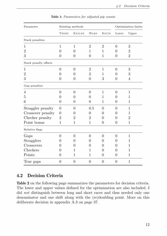
4.1 Adjusted Pip CountsTable 1 on the next page summarizes the parameters for adjusted pip counts.The parameter values are given for some existing methods and followed by thelower and upper limits specified for the optimization. The flag for “true gaps”,if set, means that a vacated point counts as a gap only if there is at least onechecker left on a higher point. Of course this definition could be changed tosomething more complicated, e. g., along the lines of Paul Lamford.

11

4.2 Decision Criteria

Table 1: Parameters for adjusted pip counts

Parameter Existing methods Optimization limits

Thorp Keeler Ward Keith Lower Upper

Stack penalties

1 1 1 2 2 0 32 0 0 1 1 0 23 0 0 0 1 0 2Stack penalty offsets

1 0 0 2 1 0 32 0 0 2 1 0 33 0 0 0 3 0 4Gap penalties

4 0 0 0 1 0 15 0 0 0 1 0 16 0 0 0 1 0 1Straggler penalty 0 0 0.5 0 0 1Crossover penalty 0 0 0 0 0 1Checker penalty 2 2 2 0 0 2Point bonus 1 1 1 0 0 1Relative flags

Gaps 0 0 0 0 0 1Stragglers 0 0 0 0 0 1Crossovers 0 0 0 0 0 1Checkers 0 1 1 0 0 1Points 0 1 1 0 0 1True gaps 0 0 0 0 0 1

4.2 Decision CriteriaTable 2 on the following page summarizes the parameters for decision criteria.The lower and upper values defined for the optimization are also included. Idid not distinguish between long and short races and thus needed only onedenominator and one shift along with the (re)doubling point. More on thisdeliberate decision in appendix A.3 on page 37.

12

4.3 Effort and Error

Table 2: Parameters for decision criteria

Parameter Existing methods Optimization limits

Thorp Keith Trice Lower Upper

Long/short breakpoint 30 0 62 – –Long race denominator 10 7 10 5 12Long race shift 2 −2 2 −3 2Short race denominator – – 7 – –Short race shift 2 – −5/7 – –Doubling point −4 −2 −3 −5 −2Redoubling point −3 −1 −2 −4 −1

4.3 Effort and ErrorWe now have identified 19 integer parameters describing an adjusted pip countand 4 integer parameters for a decision criterion. Each parameter has onlyfew possible values, since we have specified reasonable upper and lower limits:The “relative flags”, e. g., can take only 2 different values (0 or 1), while the“long race denominator” can take 8 different values, from 5 to 12. Using thisframework, there are a total of

4 · 3 · 3 · 4 · 4 · 5 · 2 · 2 · 2 · 2 · 2 · 3 · 2 · 2 · 2 · 2 · 2 · 2 · 2 = 35389440 (1)

possible combinations for an adjusted pip count and

8 · 6 · 4 · 4 = 768 (2)

possible combinations for a decision criterion. We can also combine each ad-justed pip count with each decision criterion, so overall this amounts to a“parameter space” of roughly 27 · 109 possible methods for cube handling inraces. This parameter space is too big to be evaluated completely, hence weneed a smart search technique, an optimization, to find within a finite timethe “best” combination of an adjusted pip count with a decision criterion.

We have not yet clarified the meaning of “best” in the previous paragraph:Obviously, we want a method for cube handling that results in as few errors aspossible. But we also want a method that requires as little effort as possible. Intechnical terms we are dealing with a multi-objective optimization problem.This normally involves a trade-off: The more effort, the less errors. It doesnot make sense to use a method that requires more effort and results in moreerrors. Such methods are “dominated” by others: The methods that result in

13


the fewest errors for a given effort (or, vice versa, the methods that requirethe smallest effort for a given error) are on the “Pareto front”.

In order to quantify the error, we choose a set of parameters for both, theadjusted pip count and the decision criterion, and test the resulting methodon Tom Keith’s database of endgame positions recorded on http://www.fibs.com/. For every position, the method calculates an adjusted pip countand recommends a cube action, which we compare with the correct cube actionfrom the database (as determined by roll-outs with GNU Backgammon). Anywrong decisions (in terms of lost equity) can be summed up for all positions inthe database and thus quantify the error resulting from a particular method.

Quantifying the effort is more complicated: It is not immediately clearwhether an adjusted pip count using a stack penalty of 2 and a stack penaltyoffset of 2 needs less effort than an adjusted pip count using a stack penaltyof 1 and a stack penalty offset of 1. What is clear, though, is that a gap penaltyof 0 instead of 1 makes a method simpler, because there are fewer arithmeticoperations. Likewise, lower checker penalties and lower stack penalties resultin less effort. On the other hand, higher stack penalty offsets are easier (be-cause the penalties themselves have to be applied less often). Of course, using“true gaps” means less effort, as does the use of all the “relative” flags. So for agiven method/set of parameters I ignored the signs of all the penalties/bonusesapplied by the adjusted pip count and summed up these absolute values for allpositions in the endgame database. This number of total adjustments (mea-sured in pips) was used to quantify the effort required by a particular method.

Having quantified our two objectives, we can look at some of their prop-erties that will have a big influence on choosing a successful parameter opti-mization strategy. Technically speaking, our objective functions are nonlinear(e. g., doubling a gap penalty does not necessarily double the error), multi-modal (have many local minima) and discrete (all parameters are integers).For these reasons, conventional gradient methods are likely to get stuck inlocal minima. Which is why we will start with a much better suited geneticalgorithm that explores the parameter space to identify a promising region,which we will then narrow down with a more exhaustive search, technicallya full factorial design of experiment (DOE), evaluating all of the remainingpossible parameter combinations to find the optimum cube handling method.This ensures that a least in this region of the parameter space we do not over-look the global minimum among all the local minima of the highly nonlinearobjective function.

14

5 Results

5 ResultsThe dull work of trying to choose a set of 19 parameters such that our twoobjectives (effort and error) were minimized was done by Isight, a softwaresolution for process automation and design exploration by Dassault Systèmes,the company I happen to work for. Essentially, what Tom Keith did for hismethod by trial and error was now done systematically and passed over to asoftware robot.

This exhaustive search found thousands of parameter combinations for ad-justed pip counts and decision criteria that have a smaller error than TomKeith’s original method. This is not to diminish his outstanding work, infact I consider it a great achievement to find a needle (his method with anerror of 1262) in a haystack (the huge parameter space of 27 billion combi-nations). That a more rigorous approach (using sieves and magnets, to staywith the metaphor) would find more needles was to be expected. After about5000 tested methods the optimization software found the following method(from now on termed “Isight method”):

5.1 Adjusted Pip CountsFor each player, start with a straight pip count and:

• add 1 pip for each additional checker on the board compared to theopponent;

• add 2 pips for each checker more than 2 on point 1;

• add 1 pip for each checker more than 2 on point 2;

• add 1 pip for each checker more than 3 on point 3;

• add 1 pip for each empty space on points 4, 5, or 6 (only if the otherplayer has a checker on his corresponding point);

• add 1 pip for each additional crossover compared to the opponent.

You can see that empty space is penalized in a relative sense, which meansthat, e. g., your gap on point 4 is acceptable as long as your opponent also hasa gap there. The same holds for the other high points, 5 and 6. This methoddoes not penalize stragglers, but rather if one player has more crossovers thanthe opponent. It also penalizes less checkers off in a relative sense. It does notapply bonuses for positional features like occupied points. No sophisticateddefinition of “gap” is used, just plain empty space, no matter what goes onon higher points. Finally, we have the adjusted pip counts for both players.

15

5.2 Decision Criteria

5.2 Decision CriteriaIncrease the count of the player on roll by 1/6.

• A player should double if his count exceeds the opponent’s count by atmost 6.

• A player should redouble if his count exceeds the opponent’s count byat most 5.

• The opponent should take if the doubler’s count exceeds his count by atleast 2.

You will perhaps notice that this is very similar to the wording of theKeith method. However, translating back to the terminology of section 3 onpage 10, the decision criterion uses a doubling point 4 pips shy of the point oflast take and a redoubling point 3 pips shy of the point of last take, hence the(re)doubling windows have the same size as with the Thorp method, butare shifted: The “long race denominator” is 6 and the “long race shift” is −2(in contrast to Thorp’s 10 and +2).

5.3 Effort and ErrorTable 3 compares existing methods with the method found by Isight during theoptimization. The Isight method has the smallest total error (1064), and, con-sequently, the smallest average error per decision (0.00688 equity). Not shownin the table, it also has the smallest probability of a wrong decision (7.1%).So the Isight method performs best regarding our objective to minimize theerror.

Even though the long list of items in section 5.1 on the previous page mightsuggest that the Isight method requires more effort than, say, the Keeler

Table 3: Effort and error

Method Effort (pips) Error (equity)

Total Per player Total Per decision

Thorp 2875000 27.9 3043 0.01969Keeler 313000 3.0 2253 0.01458Ward 330000 3.2 1838 0.01189Keith 379000 3.7 1262 0.00816Isight 273000 2.6 1064 0.00688

16


Table 4: Optimized parameters for adjusted pip counts

Stack penaltiesfor point

Stack penalty offsetsfor point

Gap penaltiesfor point

Total effort(Pips)

Total error(Equity)

1 2 3 1 2 3 4 5 6

2 1 1 2 2 3 1 1 1 273000 1064a2 1 0 2 2 3 1 1 1 263000 11132 1 1 2 2 3 1 1 0 261000 11482 1 1 2 2 3 0 1 1 257000 11932 1 0 2 2 3 1 1 0 251000 12142 1 0 2 2 3 0 1 1 247000 1262

a. Isight method

or Keith methods (the first does not consider gaps, the second ignores lesscheckers off, both do not take crossovers into account), the opposite is true:Gap penalties applied only if the other player has a checker there and higherstack penalty offsets save a lot of arithmetic operations. They help so muchin reducing the effort that in fact the Isight method results in less pip adjust-ments per player than the older methods.

From a multi-objective optimization point of view, you can see that theThorp method (the first adjusted pip count in history?) requires more ef-fort, but results in a higher error than the Keeler method, hence it is dom-inated by the latter. Later improvements such as from Jeff Ward or TomKeith managed to bring down the error further, but at a cost: More effortis needed. The Isight method, however, has a lower effort and error and thusdominates all former methods.

During the optimization Isight literally found thousands of methods withan error smaller than for the Keith method. Of these, six are located on thePareto front (remember, the trade-off between effort and error). They alluse the decision criterion from section 5.2 on the preceding page, a crossoverpenalty of 1, and a checker penalty of 1. Neither straggler penalty, nor pointbonus, nor true gaps are used. Gaps, crossovers, and checkers are penalized“relatively”, i. e., compared to the opponent. The other parameters are sum-marized in table 4.

Comparing lines in this table that differ only by one parameter allows usto quantify the trade-off between effort and error: Failing to penalize stackson point 3 costs about 60 points of equity (1113 versus 1064, 1214 versus1148, and 1262 versus 1193). Not penalizing a gap on point 4 costs about140 points (1193 versus 1064 and 1262 versus 1113), while not penalizing a

17

5.4 Comments on Cub-offs

Table 5: Race length and error

Race length(up to pips)

Probability of error Average error (equity)

Isight Keith Isight Keith

10 0.1287 0.1362 0.03378 0.0378020 0.1193 0.1175 0.01513 0.0156130 0.0835 0.0845 0.00741 0.0082440 0.0630 0.0694 0.00422 0.0062350 0.0500 0.0588 0.00267 0.0040960 0.0473 0.0602 0.00216 0.0036370 0.0443 0.0597 0.00144 0.0025880 0.0463 0.0510 0.00138 0.0016490 0.0606 0.0583 0.00165 0.00155

100 0.0758 0.0737 0.00247 0.00217110 0.0897 0.1004 0.00350 0.00309120 0.0278 0.1250 0.00121 0.00555

gap on point 6 costs about 90 points (1148 versus 1064 and 1214 versus 1113).The simplest method has a total error of 1262 like the Keith method, butrequires about 35% less effort. Compared with the Isight method, it still savesabout 10% effort, but has an error about 20% higher, a trade-off I do notconsider to be worthwhile.

Let us now have a closer look at the probability of a wrong cube decisionand the average error per cube decision with respect to the race length. Alladjusted pip counts, including the Isight method, are considerably more error-prone for low pip counts (roughly for a race length below 30). For these,analytical solutions are still best, but unfortunately can be very difficult andtime-consuming to calculate over the board. Having said this, table 5 showsthat the Isight method has a smaller average error (in terms of equity loss)than the Keith method for a race length up to 80 pips. From 80 pips up to110 pips the Keith method is slightly more accurate, whereas in very longraces (longer than 110 pips) again the Isight method has the edge. For racesup to 10 pips, from 21 pips to 80 pips, and above 110 pips the Isight methodis also less likely to result in a wrong cube decision.

5.4 Comments on Cub-offsEven though for very short races both the likelyhood of a wrong cube decisionand the size of the error increase considerably, it is interesting to push the

18

6 Alternative Approaches

envelope of the Isight method and assess its performance for “cub-offs”, a termcoined by Danny Kleinman for bear-off positions with at most 2 checkersleft per player. Overall, there are 729 cub-offs, and for 405 cub-offs the playeron roll has a CPW between 50% and 95%.

The Isight method yields wrong decisions for about 12% of these, a sur-prisingly small fraction. The average error per decision is only about 0.025.Unless you feel very confident about memorizing the complete cub-offtables available on the internet (http://www.bkgm.com/articles/Koca/CuringYourShortBearoffBlues.html), or, alternatively, you feel very con-fident about doing the math over the board (remember, without pencil andpaper, but including potential redoubles . . . ), it thus might be a reasonableapproach to (ab)use the Isight method even for cub-offs.

6 Alternative Approaches6.1 EPC ApproximationsA concept quite different from adjusted pip counts is the EPC invented byWalter Trice, see the article mentioned in section 1 on page 3. In brief,the EPC of a particular position is the average number of rolls needed tobear off completely, multiplied by the average number of pips in a roll (whichis 49/6).

The problem with this approach is to determine the average number ofrolls, since we do not have exact EPCs over the board. While this can easilybe estimated for “rolls” positions (ace-point stacks) or low-wastage “pips”positions, in general, for the many positions that fall in between, the procedureis far from easy: It requires remembering the wastage for quite a number ofcases, a good deal of experience and feeling for the position, or “synergy”wizardry (see Douglas Zare’s article mentioned in section 2.2 on page 5,which unfortunately does not explain the details). To me, the whole concept,while very elegant from a mathematical point of view, seems rather fuzzy andnot very well suited for a strict algorithmical solution, which is much more tomy liking.

But perhaps could such an algorithm be found by assessing positionalfeatures and adjusting for them (as explained in section 2 on page 4), sothat we do not end up with some arbitrary adjusted pip count, but ratherwith something approximating the EPC as closely as possible? This approachseems to be quite promising and was Joachim Matussek’s idea, see hisarticle mentioned in section 1 on page 3. He applies stack penalties (for allpoints from 1 to 6), adds a further pip if any stack is at least 4 checkers high

19

6.1 EPC Approximations

and yet another pip if any stack is at least 6 checkers high. His method alsouses a “synergy” effect, i. e., it subtracts a bonus of 1 pip if point 1 is occupied,but at least 3 other points are occupied as well. Another distinct feature isthe use of a constant penalty applied always, since every position will wasteat least a couple of pips. He uses 4.5 pips for this purpose. His method resultsin an average EPC error per player per position of 1.70 pips (for each positionin the database EPCs for both players need to be approximated).

So I augmented Tom Keith’s database of endgame positions with EPCsas determined by GNU Backgammon (which fortunately very well supportssuch automation of tasks by scripting). Then I changed the objective functionof the optimization problem: Now I did not want to minimize the total cubeerror, but rather the difference between the adjusted pip count and the correctEPC from the database. I also had to introduce additional parameters for thesynergy effect and the constant penalty. Then I could start the optimizationprocess. This is what Isight found as an EPC approximation:

For each player, start with a straight pip count and:

• add 5 pips;

• add 2 pips for each checker on point 1;

• add 1 pip for each checker on point 2;

• add 1 pip for each checker on point 3;

• subtract 1 pip if point 1 and at least 3 other points are occupied.

This method allows to estimate the EPC for a player’s position with an av-erage error of only 1.04 pips, hence it has a smaller total error and requires lesseffort than Joachim Matussek’s method, which uses non-integer penaltiesfor all home board points.

While an approximation for EPCs is certainly nice to have, our main pur-pose is cube handling in races, so we need to combine our “adjusted pip count”(which by now has become an EPC approximation) with a suitable decisioncriterion. Indeed there is one, somewhat hidden in Walter Trice’s book,with a denominator of 49/6 and a shift of −3. Combining this criterion withthe EPC approximation from above, we get a total error of 1909 (now a totalcube error in terms of equity, not an EPC error in terms of pips), much worsethan the Keith method (1262) or the Isight method (1064) from section 5on page 15. The question why this result is so bad needs some investigation.

The problem with EPCs, even if you have an algorithm to estimate themover the board, is that Walter Trice’s decision criterion is very sensitiveto the EPCs, since it has a doubling point only 2 pips shy of the point of last

20

6.2 CPW Approximations

Table 6: EPC approximations with Walter Trice’s decision criterion

EPC approximation EPC error per player(Pips)

Total cube error(Equity)

Isight 1.04 1909Matussek 1.70 1498Exact ±1.5 0.75 1294Exact ±1.3 0.65 1067Exact ±1.0 0.50 800Exact 0.00 401

take. You can imagine that being 2.5 pips off with your EPC approximation caneasily be the difference between “No double, take” and “Redouble, pass”. Thisreasoning could be confirmed by hard numbers: I took the exact EPCs fromthe database and added/subtracted uniformly distributed random numbers.The resulting “EPC approximations” were combined with Walter Trice’sdecision criterion to determine the cube action. As usual, the total error wassummed up for all positions in the database, see table 6.

The results are disappointing: In order to get a total cube error compara-ble to the Isight method (1064) from section 5 on page 15, we need an EPCapproximation with an average EPC error of about 0.65, which is probablyvery difficult to achieve. However, assuming we had the exact EPCs, WalterTrice’s criterion gives extremely accurate cube decisions. Unfortunately, itdoes not work very well with the EPC approximations we have found so far.This is an area with room for improvements in the future. Maybe someonewill find an approximation that is accurate enough to be useful in combinationwith Walter Trice’s criterion, which is definitely not the culprit, see thetotal error of only 401!

An interesting detail is that Joachim Matussek’s EPC approximation,though worse than Isight’s, results in a smaller total cube error. We cantake this as a hint that adjusted pip count and decision criterion needto be matched. However, Joachim Matussek does not employ WalterTrice’s criterion (his article does not deal with cube decisions at all), butrather uses the EPC approximation he found to approximate the CPW. Thisleads us to yet another approach.

6.2 CPW ApproximationsIf we had them, exact CPWs in combination with percentages defining thedoubling/redoubling window would be even more accurate than using exact

21


EPCs with Walter Trice’s criterion. According to Tom Keith the totalcube error would be 201. He also mentions:

Unfortunately, it is usually harder to accurately estimate CPWthan it is to make correct cube plays, so this method is reallymore of academic interest.

Fortunately, Tom Keith is not right. Let us see how CPW approximationswork.

The formula Joachim Matussek uses to approximate the cubelessprobability p of winning (in percent) for a race length l (roller’s pip count)and a roller’s lead ∆l is

p(l, ∆l) = 50 % + v(l) ·(

∆l + 4912

), (3)

with v being the value of a pip (depending on the roller’s pip count). Thisseems reasonable, since it has the nice property of giving 50% winning chancesif the roller is about 4 pips behind (half a roll, 49/12), a CPW we know forsome decades to be true for a wide range of race lengths. Both roller’s andnon-roller’s pip counts can be (and usually are) adjusted. Complications arisewhen the value of a pip needs to be factored in. Joachim Matussek givesa table for this, which needs further adjustments for positions in which at leastone player has a “rolls” position rather than a “pips” position.

Since I did not want to memorize and adjust values from a look-up table, Ithought about a table published by Tom Keith showing the CPW directlyas a function of race length and lead, http://www.bkgm.com/rgb/rgb.cgi?view+1203. My idea was to approximate it using a linear regression

p(l, ∆l) = b− l

dC+ v ·∆l , (4)

for which the base probability b, the CPW denominator dC, and the (now con-stant) value of a pip v needed to be determined. Initial tests of fitting TomKeith’s table with this approach were promising. Using optimization soft-ware, this was again an easy task. With the CPW error (absolute differencebetween the correct CPW as rolled out by GNU Backgammon and its approx-imation) as an objective to minimize, Isight found the following method:

p = 77− l

4 + 2∆l (5)

This CPW approximation has an average CPW error of 4.13 percentage points.The next optimization problem for Isight was to find parameter values (i. e.,

22


Table 7: Parameters for CPW approximations

Parameter Lower Upper Unit

Base probability b 50 100 %CPW denominator dCPW 2 10 –Pip value v 1 6 %Doubling point 65 75 %Redoubling point 69 75 %Point of last take 75 80 %

percentages) for the doubling point, the redoubling point, and the point oflast take such that combined with this CPW approximation the total errorfor the cube decisions was minimized. The parameters and their limits forthese two runs are shown in table 7. The limits were chosen using a mixtureof guesswork, gut feeling, and old backgammon lore. They should reasonablybracket the optimum. The first three parameters were used in the first runfor the optimization of the CPW approximation, the second three parameterswere used in the second run for the optimization of the (re)doubling window.Isight found that with a doubling point of 68%, a redoubling point of 70%,and a take point of 76% this CPW approximation gives a total cube errorof 1264. This is roughly on par with the Keith method (1262), but worsethan the Isight method (1064) from section 5 on page 15.

So I started another run, this time as a multi-objective optimization withboth the CPW error and the total cube error to be minimized simultaneously,using all parameters from table 7. The parameter limits were unchanged.Isight then found the following CPW approximation for a roller’s pip count land a roller’s lead ∆l:

p = 80− l

3 + 2∆l (6)

The (CPW-based) decision criterion uses the following percentages for thedoubling and redoubling window to determine the cube action:

• p < 68: No double, take.

• 68 ≤ p < 70: Double, take.

• 70 ≤ p ≤ 76: Redouble, take.

• p > 76: Redouble, pass.

23

6.3 Methods for Matches

Even though (due to the multi-objective nature of the optimization task)this method compromises a little bit on average CPW error (4.26 percentagepoints in comparison to the former 4.13), it does much better than equation (5)when it comes to cube errors. It fact, it gives exactly the same total cube errorof 1064 as the Isight method. Even the decimal places (omitted here) matchedperfectly. Could this be pure chance? Probably not, and we will see why inthe next subsection.

6.3 Methods for MatchesThe equations for CPW approximation somehow reminded me on ChuckBower’s interpolation for the Thorp method. In case you are not famil-iar with it, this is how it works (his article can be found at http://www.bkgm.com/rgb/rgb.cgi?view+158): If a Thorp count T of −2 correspondsto the doubling point (say 70%) and a Thorp count T of +2 corresponds tothe point of last take (say 78%), then a simple linear interpolation will give aCPW approximation:

p = 74 + 2T (7)

The Isight method combines the adjusted pip count from section 5.1 onpage 15 with the decision criterion from section 5.2 on page 16. This results ina total cube error of 1064. If now the same adjusted pip count is combined withthe decision criterion from the previous subsection, we also get a total cubeerror of 1064. Hence I had a strong suspicion that there might be a generalway to transform a decision criterion based on (re)doubling points and thepoint of last take into a decision criterion based on percentages and the CPW.A criterion of the latter form has the big advantage that it is suited for matchplay, in which the doubling window might be far away from the usual valuesfor a money session. And indeed, there is a correspondence, and the reasoningand the transformation are quite easy, since the decision criteria have all beenparametrized earlier.

You might recall from section 3.1 on page 10 that we get the point of lasttake by increasing the roller’s pip count l by a fraction of the roller’s pip count(determined by the “long race denominator” dl) and adding a further shift s.If the non-roller, who has a pip count of l + ∆l, is precisely at this point oflast take with a CPW of pt (e. g. 78%), we can state the following implication:

l + l

dl+ s = l + ∆l ⇒ p = pt (8)

Since the doubling point is sd pips shy of the point of last take (sd beingnegative), which corresponds to a CPW of pd (e. g. 70%), we can state the

24


following implication:

l + l

dl+ s + sd = l + ∆l ⇒ p = pd (9)

After subtracting l from both sides of these two equations, linear interpolationgives the following “transformation formula”:

p = pd − (pt − pd)∆l −

(l

dl+ s + sd

)sd

(10)

Let us try this formula on the Isight decision criterion presented in sec-tion 5.2 on page 16. The long race denominator dl is 6, the shift s is −2, andthe doubling point sd is −4. With a CPW of 70% at the doubling point and78% at the point of last take this results in

p = 70− (78− 70)∆l −

(l6 − 2− 4

)−4 , (11)

which after a little bit of algebra turns out as

p = 82− l

3 + 2∆l . (12)

Does not this look familiar yet? Not quite? Well, using this CPW approxima-tion with a doubling window from 70% to 78% will by design give exactlythe same cube decisions as using 80 instead of 82 for the constant term in theCPW approximation with a doubling window from 68% to 76%. All numberswill just be shifted by 2%. So finally we are back to

p = 80− l

3 + 2∆l (13)

with a (re)doubling window of 68%, 70%, and 76%. It will give us a totalcube error of 1064 as well, but has a slighly smaller CPW error than equa-tion (12) and is thus better suited for match play, in which the percentagesused for the (re)doubling window will have to be adapted based on score. Thetransformation formula thus has provided a very nice connection between theIsight solutions for the two (originally unrelated) optimization problems.

If my framework for adjusted pip counts and decision criteria can be seenas a generalization of Tom Keith’s work, my transformation formula canbe seen as a generalization of Chuck Bower’s work: Once you have anadjusted pip count and a decision criterion using a point of last take and a(re)doubling window of a particular size, you can easily convert it into an

25


Table 8: CPW approximations with transformation formula

Method b dC v Doublingpoint

Redoublingpoint

Pointof lasttake

Totalerror

AverageCPWerror

% – % % % % – %

Thorp1 74 5 2 70 72 78 4433 5.72Keith2 86 7/4 4 70 74 78 1262 10.09Matussek3 90 49/24 4 70 74 78 1498 10.86Matussek4 90 2 4 70 74 78 1485 10.75Isight 77 4 2 68 70 76 1264 4.13

80 3 2 68 70 76 1064 4.2682 3 2 70 72 78 1064 4.5485 2 3 68 71 79 1049 8.27

1. Without Bill Robertie’s enhancement (no long/short race distinction)2. Necessary rounding down not represented by parameter values3. Combined with Walter Trice’s decision criterion for EPC approximations4. Like 3., but rounded value used for denominator

equivalent method working with percentages. Both methods will by designresult in exactly the same cube action in a money session, however the latterwill also work for match play. This is important for tournament players, in-deed I was specifically asked by former German champion Tobias Hellwagwhether I had such a method in my theory bag. Now I do . . .

In case you are flirting with applying the transformation formula to yourfavorite Thorp or Keith method (as an “exercise for the reader”), a wordof warning is in place: Of course this is possible, but for both methods it is notas straight forward as for the Isight method. The Thorp method (at leastin its version enhanced by Bill Robertie) distinguishes between long andshort races, while the Keith method does some rounding down during thedefinition of the point of last take. These features complicate things a littlebit, hence I cheated somewhat with the numbers in table 8: The results for theCPW-based version of the Thorp method hold for his original formulation,i. e., without distinction between long and short races. For the Keith methodyou need to know where the rounding takes place:

p = 86− 4 ·⌊

l

7

⌋+ 4∆l (14)

By the way, as good as the Keith method is, for match play its average CPW

26

7 Discussion

error is surprisingly high. This perhaps explains Tom Keith’s quote fromthe beginning of section 6.2 on page 21. The same holds for Joachim Ma-tussek’s method, which was meant as an EPC approximation. As a detail,this method slightly benefits both in terms of total cube error and CPW error,if instead of the exact value for the CPW denominator (49/24, resulting fromthe transformation formula) a rounded value of 2 is used.

The methods found by Isight all do a very good job regarding the total cubeerror. The first three of them should be familiar from this and the previoussubsection. The last one was not yet mentioned, it gives the smallest totalcube error of all CPW-based methods found by Isight, however its CPW ismuch higher than for the other ones, which is bad for match play.

7 DiscussionThis paper presented a general, parametrized framework for adjusted pipcounts and decision criteria for cube handling in pure races without contact.The positional features considered for adjusted pip counts were checkers al-ready borne off, high stacks on low points, gaps on high points, and crossoversneeded before the bear-off starts. For decision criteria a distinction betweenlong and short races was considered, but turned out to be unnecessary, sincelong races are rare. The point of last take was determined using a denominatorand a further shift. In turn, doubling and redoubling point were shifted fromthe point of last take.

Having the framework in place, lower and upper limits for all the parame-ters were specified. Two objectives were defined: The total cube error shouldbe minimized (tested against a database containing the correct cube actionsfor around 50000 real life endgame positions), and the total effort should beminimized (quantified using the total number of pips added/subtracted bythe adjustments). Several multi-objective optimizations were done using thesoftware solution Isight. First, an adjusted pip count and a decision crite-rion were found. The resulting method for cube handling in races has botha lower effort and error than existing methods. It can be reasonably usedeven for cub-offs. It is crucial that the decision criterion be valid for positionswith wastage in order to match an adjusted pip count successfully. Second, amethod for approximating EPCs was found, with both a lower effort and EPCerror than existing methods. This method is not suitable for cube handling.Third, a method for approximating CPW was found, with a decision criterionthat resulted in exactly the same cube action as the method found before.

Indeed, a connection between these two methods was found: The trans-formation formula describing it can be used to convert any decision criterion

27

8 Summary

based on a point of last take and a (re)doubling window into an equivalentmethod working with percentages. This allows for the use in match play, forwhich the percentages will have to be adapted based on score.

8 Summary• To approximate EPCs, start with a straight pip count for each player.

◦ Add 5 pips.◦ Add 2 pips for each checker on point 1.◦ Add 1 pip for each checker on point 2.◦ Add 1 pip for each checker on point 3.◦ Subtract 1 pip if point 1 and at least 3 other points are occupied.

• To decide on cube action, start with a straight pip count for each player.

◦ Add 1 pip for each additional checker on the board compared tothe opponent.◦ Add 2 pips for each checker more than 2 on point 1.◦ Add 1 pip for each checker more than 2 on point 2.◦ Add 1 pip for each checker more than 3 on point 3.◦ Add 1 pip for each empty space on points 4, 5, or 6 (only if theother player has a checker on his corresponding point).◦ Add 1 pip for each additional crossover compared to the opponent.◦ With your adjusted pip count l and your lead ∆l (can be negative),

p = 80− l

3 + 2∆l

is your approximated CPW. The cube action for money is:◦ p < 68: No double, take.◦ 68 ≤ p < 70: Double, take.◦ 70 ≤ p ≤ 76: Redouble, take.◦ p > 76: Redouble, pass.◦ Adapt (re)doubling window according to match equity calculationsin tournaments.

28

A Appendix

A AppendixA.1 ExamplesAfter so much generalization, parametrization, design space exploration,multi-objective optimizations, equations, interpolation, transformations, andapproximations of various acronyms it is high time to apply the Isight methodto some examples. Except for one position (“pips” versus “rolls”), the follow-ing examples have all been taken randomly from Tom Keith’s database ofendgame positions played on FIBS. We will apply the adjusted pip count andthe decision criterion based on the CPW approximation to all of them. In ad-dition, the summary table below each figure will also give the values from theEPC approximation. The outcome will be compared with the correct resultsfrom GNU Backgammon.

The purpose of these examples is not the verification of the methods,which has already been done by testing them on the full database, and theresults of this have been presented in the main part of this paper. Instead,these examples should rather be seen as exercises in applying the methodsand as a way to resolve any ambiguities (hopefully few) still present in theirformulation.

In figure 5 on page 31 the straight pip count is 86 versus 90. Both playershave to bear off the same number of checkers, so no checker penalty is applied.No player has more than 2 checkers on his point 1, more than 2 checkers onhis point 2, or more than 3 checkers on his point 3, so no penalties needto be applied for stacks. No player has gaps on his points 4, 5, or 6, so nopenalties need to be applied for gaps. White has 4 checkers with 1 crossoverand 1 checker with 2 crossovers, in total 6 crossovers. Red has 5 checkers with1 crossover each, in total 5 crossovers. Hence White gets 1 pip penalty. Theadjusted pip count is 87 versus 90, so the race length is 87 pips and the leadis 3 pips. This results in a CPW for White of 80− 87/3 + 2 · 3 = 57 % < 68 %.The cube action is thus “No double, take”. A rollout with GNU Backgammonconfirms the cube action, but gives a CPW of 65.6%.

In figure 6 on page 31 Red has borne off 2 checkers less than White,so Red gets 2 pips penalty. Red also has 5 checkers on point 2, 3 more than“allowed”, so Red gets another 3 pips penalty. White has 5 checkers on point 3,2 more than the “allowed” 3, so White gets 2 pips penalty. White has a gapon point 4, whereas Red does not, so White gets 1 pip penalty. On the otherhand, Red has a gap on point 6, whereas White does not, so Red gets one pippenalty, too. Red has 1 additional crossover and so gets another 1 pip penalty.The adjusted pip count is 53 versus 62. White’s lead is 9 pips. His CPW is

29

A.1 Examples

80 − 53/3 + 2 · 9 ≈ 79.7 % > 76 %. The cube action is thus “Redouble, pass”.This is confirmed by GNU Backgammon, which reports a CPW of 80.2%.

In figure 7 on page 32 White gets 1 pip penalty due to 12 checkers offagainst 13 for Red. There are no stacks, but gaps: 1 pip gap penalty for Redon point 4, 1 pip gap penalty for White on point 5, no gap penalty on point 6.No crossovers left. The adjusted pip counts become 10 versus 11, White’s leadis 1 pip. His CPW is 80 − 10/3 + 2 · 1 ≈ 79.7 % > 76 %. The cube action isthus “Redouble, pass”. GNU Backgammon confirms this and reports a CPWof 84%.

In figure 8 on page 32, the Isight method is abused for a cub-off. Whitegets an additional pip for its 2 checkers left against 1 checker for Red. No stackpenalties, but 1 pip gap penalty for Red on point 4 (since White has occupiedits point 4). No crossover penalties. The adjusted pip count is 7 versus 4.The race length is 7, White’s lead is −3. His CPW is 80 − 7/3 + 2 · (−3) ≈71.7 % ≥ 70 %. Since 71.7 % ≤ 76 %, the cube action is “Redouble, take”.GNU Backgammon also reports “Redouble, take”, but a CPW of only 63.9%.

In figure 9 on page 33, only Red gets 1 pip penalty, since White hasborne off 1 more checker. No penalties for stacks, gaps, or crossovers. Theadjusted pip count becomes 52 versus 60. White’s lead is 8 pips. His CPW is80− 52/3 + 2 · 8 ≈ 78.7 % > 76 %. The cube action becomes “Redouble, pass”,confirmed by GNU Backgammon, which reports a CPW of 80.5%.

In figure 10 on page 33, an extreme “pips versus rolls” position, the straightpip count (30 versus 15) is highly misleading. Red gets 4 pips penalty for hisfewer checkers borne off. Red gets 6 pips penalty for his 3 checkers “too many”on point 1. Red also gets 3 pips penalty for his 3 checkers “too many” onpoint 2. Finally, Red gets 3 pips penalty for his gaps on points 4, 5, and 6, allof which White has occupied on his side of the board. The adjusted pip countbecomes 30 versus 31. White leads by 1 pip! His CPW is 80 − 30/3 + 2 · 1 =72 % ≥ 68 %. The cube action is “Double, take”. GNU Backgammon confirmsthe cube action and gives a CPW of 67.7%.

In figure 11 on page 34 White gets 2 pips penalty for his third checkeron point 1. He also gets 1 pip penalty for his third checker on point 2.Red accordingly gets 4 pips penalty for his stack on point 2 (4 checkers“too high”, 6 instead of 2). No penalties for crossovers or gaps (becauseboth players have vacated their points 4, 5, and 6, there are no “relative”gaps). The adjusted pip count is 18 versus 18, White’s lead is 0. His CPW is80 − 18/3 + 2 · 0 = 74 % > 68 %. The cube action becomes “Double, take”,confirmed by GNU Backgammon, which reports a CPW of 74.7%.

Figure 12 on page 34 concludes this appendix with two example positions,which can be used to test your understanding of the methods. For these, onlythe final results are presented, but no complete summary tables. Good luck!

30

A.1 Examples

White Red

Straight 86 90PenaltiesCheckers 0 0Stack on 1 0 0Stack on 2 0 0Stack on 3 0 0Gap on 4 0 0Gap on 5 0 0Gap on 6 0 0Crossovers 1 0Adjusted 87 90Prediction (Isight method)CPW (%) 57.0 43.0Cube action No double TakeEPC 95 97Solution (GNU Backgammon)CPW (%) 65.6 34.4Cube action No double TakeEPC 95.5 98.3

Figure 5: Long race

White Red

Straight 50 55PenaltiesCheckers 0 2Stack on 1 0 0Stack on 2 0 3Stack on 3 2 0Gap on 4 1 0Gap on 5 0 0Gap on 6 0 1Crossovers 0 1Adjusted 53 62Prediction (Isight method)CPW (%) 79.7 20.3Cube action Redouble PassEPC 63 68Solution (GNU Backgammon)CPW (%) 80.2 19.8Cube action Redouble PassEPC 62.0 68.5

Figure 6: Medium-length race

31

A.1 Examples

White Red


Figure 7: Short race

White Red

Straight 6 3PenaltiesCheckers 1 0Stack on 1 0 0Stack on 2 0 0Stack on 3 0 0Gap on 4 0 1Gap on 5 0 0Gap on 6 0 0Crossovers 0 0Adjusted 7 4Prediction (Isight method)CPW (%) 71.7 28.3Cube action Redouble TakeEPC 12 9Solution (GNU Backgammon)CPW (%) 63.9 36.1Cube action Redouble TakeEPC 11.1 8.2

Figure 8: Cub-off

32

A.1 Examples

White Red


Figure 9: “Pips” position

White Red

Straight 30 15PenaltiesCheckers 0 4Stack on 1 0 6Stack on 2 0 3Stack on 3 0 0Gap on 4 0 1Gap on 5 0 1Gap on 6 0 1Crossovers 0 0Adjusted 30 31Prediction (Isight method)CPW (%) 72.0 28.0Cube action Double TakeEPC 35 35Solution (GNU Backgammon)CPW (%) 67.7 32.3Cube action Double TakeEPC 36.3 36.2

Figure 10: “Pips versus rolls” position

33

A.1 Examples

White Red

Straight 15 14PenaltiesCheckers 0 0Stack on 1 2 0Stack on 2 1 4Stack on 3 0 0Gap on 4 0 0Gap on 5 0 0Gap on 6 0 0Crossovers 0 0Adjusted 18 18Prediction (Isight method)CPW (%) 74.0 26.0Cube action Double TakeEPC 31 29Solution (GNU Backgammon)CPW (%) 74.7 25.3Cube action Double TakeEPC 29.9 30.0

Figure 11: “Rolls” position

White Red

Prediction (Isight method)CPW (%) 67.7 32.3Cube action No redouble TakeSolution (GNU Backgammon)CPW (%) 69.0 31.0Cube action No redouble Take

White Red

Prediction (Isight method)CPW (%) 81.0 19.0Cube action Double PassSolution (GNU Backgammon)CPW (%) 83.5 16.5Cube action Double Pass

Figure 12: Two quiz positions

34

A.2 Combinations of Counts and Criteria

A.2 Combinations of Counts and CriteriaThe parametrization of adjusted pip counts and decision criteria all using thesame (or a very similar) framework allowed to test a lot of combinations.During my hunt for an improved method for cube handling I implemented thefollowing adjusted pip counts for testing:

• Straight (not adjusted)

• Thorp

• Keeler

• Ward

• Keith

• Isight (adjusted pip count, EPC approximation, and CPW approxima-tion)

• Matussek (EPC approximation and CPW approximation)

The decision criteria I implemented for testing were:

• Robertie

• Thorp (with Robertie’s enhancement)

• Kleinman metric

• Chabot

• Trice (based on point of last take, i. e., Rule 62, or based on EPCs,using the “hidden” criterion given in his book)

• Nack-57

• Nack-58

• Keith (based on point of last take or based on CPW, using the per-centages given in his article)

• Isight (based on point of last take or based on CPW)

35

A.2 Combinations of Counts and Criteria

Table 9: Combinations and error

Adjusted pip count

Decision criterion Straight Thorp Keeler Ward Keith Isight Matussek

Robertie 9376 4753 3422 2839 3943 2856Thorp 7784 3438 2298 1838 2360 1709Kleinman 8301 4026 2466 1928 3031 1865Chabot 7819 2745 2118 1760 1518 1369Trice (Rule 62) 7954 3527 2143 1702 2016 1424Nack-57 7944 3503 2133 1684 1988 1415Nack-58 7948 3558 2140 1687 2007 1417Keith 7529 2861 1988 1835 1262 1233Isight 7228 2749 1743 1438 1474 1064 1934aKeith (CPW) 1113b 2199cTrice (EPC) 1909d 1498e

a. Matussek’s CPW approximation, then Isight’s percentagesb. Isight’s CPW approximation, then Tom Keith’s percentagesc. Matussek’s CPW approximation, then Tom Keith’s percentagesd. Isight’s EPC approximation, then Walter Trice’s EPC-based criterione. Matussek’s EPC approximation, then Walter Trice’s EPC-based criterion

Having all these building blocks available, it was very easy to test, e. g., whichadjustments are best suited if you want to use the Kleinman metric asyour decision criterion. I also checked combinations with Walter Trice’sRule 62, Nack Ballard’s “Nack-57” and “Nack-58” (co-authored by NeilKazaross), and a fairly new method by Michelin Chabot. The totalcube error for various combinations is shown in table 9.

From the data, a couple of things are apparent: A straight pip countis much worse than the Thorp method, which in turn is worse than theKeeler method, which in turn is worse than the Ward method. This isjust an extension of the work Tom Keith did in his investigation. His ownadjusted pip count is typically worse than the Ward method, except whencombined with his own decision criterion (which is of course the thing to do) orthe very similar one by Michelin Chabot. The Ward method in turn isworse than the Isight method, except when combined with Bill Robertie’sdecision criterion.

You can also see that neither the metric by Danny Kleinman, norWalter Trice’s Rule 62 in combination with Jeff Ward’s adjustments,nor Nack Ballard’s methods, nor Michelin Chabot’s method come

36

A.3 Long Race or Short Race?

close to what Tom Keith had achieved already 10 years ago. The sameholds for the alternative approach of approximating EPCs and using an ap-propriate decision criterion suited for them.

Almost all decision criteria benefit when they are combined with Isight’sadjusted pip count. And almost all adjusted pip counts benefit when combinedwith Isight’s decision criterion. The best choice (in terms of minimum totalerror) is to combine Isight’s adjusted pip count with Isight’s decision criterion.Since Isight optimized both things simultaneously, this is a strong rationalefor matching adjusted pip count and decision criterion.

It is also interesting to compare Walter Trice’s Rule 62 with Nack-57/58 and the Chabot method: These decision criteria are all related tothe “gold standard table” (more on this in the next section), which is repro-duced exactly by Nack-57/58, but only approximated by Rule 62. MichelinChabot in turn only approximates Rule 62 (by using a denominator of 8,no shift for the point of last take, and omitting the long/short race distinc-tion), so one would expect to see the highest total error for Chabot, followedby Trice and Nack-57/58. However, for most of the adjusted pip counts,Chabot fares best of these four decision criteria. Why?

A possible explanation is that the “gold standard table” is valid only forlow-wastage positions. However, like in the database of endgames played onFIBS, positions frequently show considerable wastage. This of course calls foradjusted pip counts, so the poor performance even of the “exact” Nack-57/58is only to be expected. Getting the necessary adjustments right and matchingthem with an adequate decision criterion is more important than trying tosqueeze out the last bit of equity using square roots and a distinction betweenlong and short races. We will deal with the latter topic next.

A.3 Long Race or Short Race?Why should one care about the distinction between long and short races(which introduces 3 additional parameters, i. e., the breakpoint between longand short races, the “short race denominator”, and the “short race shift”)?Well, Walter Trice came up with a table for money cube action in low-wastage positions. He was an expert in racing theory, so his table has beentermed “gold standard table”. It contains the maximum pip deficit for thenon-roller (point of last take) depending on the roller’s pip count. The corre-sponding graph is plotted in figure 13 on the next page.

Walter Trice’s “Rule 62” is able to generate this table (at least ap-proximately) from a couple of simple arithmetical rules. Nack Ballarddevised a new arithmetical rule, “Nack-57”. Either this or its modification“Nack-58” manage to reproduce the table exactly (the “winner” is not yet clear

37


Figure 13: “Gold standard table” approximations with straight lines

Table 10: Optimized parameters for decision criteria

Denominator Shift Total error

3 −8 30344 −4 17785 −3 11456 −2 10647 −1 11448 −1 13299 0 1412

10 0 159711 1 175012 1 186013 1 200214 1 216115 1 232116 2 2403

38


from the rollouts), see http://www.bgonline.org/forums/webbbs_config.pl?noframes;read=59714. Both methods contain a distinction between longand short races with the breakpoints being, you guessed it, 62 and 57, re-spectively. You can see from figure 13 on the preceding page that methodswithout this distinction give a poorer fit to the data, e. g., the old Thorpmethod (without Bill Robertie’s enhancement) with its long race denom-inator of 10 (which corresponds to a slope of 1/10) matches well only for thehigher pip counts, while Isight’s method with its long race denominator of 6matches the lower pip counts well. Tom Keith’s method with its long racedenominator of 7 is a compromise and does a good job overall. This lookedlike just another optimization problem well suited for an investigation withIsight: For a simple decision criterion without distinction between long andshort races, table 10 on the previous page lists the best shift value for eachdenominator along with the resulting total cube error. The lowest total errorof 1064 is achieved with a denominator of 6 and a shift of −2, correspondingto the Isight method already presented in section 5.2 on page 16.

But if the Isight method is a rather poor fit of the “gold standard table”for the higher pip counts, three questions arise:

1. Why does it perform so well in comparison with other methods?

2. Why does it perform better than even the exact representation of the“gold standard table” by Nack-57/58?

3. Could it be improved even further by reintroducing the distinction be-tween long and short races?

First, it performs so well because most of the endgames are rather short,see the distribution of the race length for Tom Keith’s database in figure 14on the next page: About 50% of the races are shorter than 40 pips, 90% areshorter than 70 pips, and 95% are shorter than 75 pips. So fitting the straightline approximating the “gold standard table” to the shorter races pays in termsof increased accuracy. It is a number’s game, so better adapt your heuristicsto situations occuring frequently than to rather rare cases.

Second, Isight’s decision criterion works better than Nack-57/58 for tworeasons: The “gold standard table”, as already mentioned, refers to low-wastage positions. If we define a low-wastage position as a position thatdoes not require any adjustments by the Isight method, then Tom Keith’sdatabase of around 50000 endgame positions contains only about 3000 of those(around 6%). A “gold standard table” that cannot be reasonably applied topositions with wastage loses a lot of its value. The other reason is that decisioncriterion and adjusted pip count need to be matched: Imagine two different

39


Figure 14: Race length and positions

methods for adjusting pip counts, one adding 100 pips per checker still on theboard, while the other works with a straight pip count, decreased further byapplying a bonus for a smooth position. It is obvious that these two methodsmust be paired with quite different decision criteria in order to give accu-rate cube decisions. Isight (and probably Tom Keith, too) optimized bothadjusted pip count and decision criterion simultaneously.

Third: Yes, but only slightly. With 50 pips as the breakpoint, 5 as the shortrace denominator, −3 as the short race shift, 10 as the long race denominator,and 2 as the long race shift, you will get a total error of 1041, in comparisonwith the original 1064, at the cost of 3 additional parameters (and numbersto memorize). Applying the transformation formula then gives

p ={

84− 25 l + 2∆l, l ≤ 50

74− 15 l + 2∆l, l ≥ 50

(15)

as the corresponding CPW-based decision criterion with a (re)doubling win-dow of 70%, 72%, and 78%, to be adapted in match play. To me, this methodis not worth the effort, so it is mentioned just for reference. You decide.

40

Improved Cube Handling in Races: Insights with · PDF fileImproved Cube Handling in Races:...

Documents

Transcript of Improved Cube Handling in Races: Insights with · PDF fileImproved Cube Handling in Races:...