IMPLICATION OF INFORMATION DISRUPTION TO SUPPLY …Olatunde Amoo Durowoju Norwich Business School...

IMPLICATION OF INFORMATION DISRUPTION

TO SUPPLY CHAIN IMPROVEMENT

STRATEGY DECISION - AN ENTROPY

PERSPECTIVE

By

Olatunde Amoo Durowoju

Norwich Business School

Faculty of Social Sciences

University of East Anglia

Thesis submitted in fulfilment of the requirement for the degree of

Doctor of Philosophy in Management Research

June 2014

Supervisors: Dr Hing Kai Chan and Dr Xiaojun Wang

© This copy of the thesis has been supplied on condition that anyone who consults it

is understood to recognise that its copyright rests with the author and that use of any

information derived there from must be in accordance with the current UK Copyright

Law. In addition, any quotation or extract must include full attribution.

ii

DEDICATION

To my wife, Esther Preeti, and son, Samuel Boluwatife Tanay

To my Parents, Chief and Chief Mrs Durowoju

To my father-in-law, Rev. Irwin Lall and late Mother-in-law, Mrs Vijaya Lall

iii

ACKNOWLEDGEMENT

I would like to thank Dr Hing Kai Chan and Dr Xiaojun Wang for their phenomenal

supervision throughout the PhD process. Their comments and positive criticism have

been invaluable to the completion of this study. Being the primary supervisor, Dr

Chan’s work ethic regarding my PhD supervision has been nothing short of

extraordinary. He has given me something to aspire to as a researcher and I am

grateful for the benchmark he now represents. As my secondary supervisor, Dr

Wang was very instrumental in guiding my thought process and has helped honed

my critical thinking ability, for which I am very grateful. Beyond that, their pastoral

role has been inspirational, getting me through the lows of the PhD process. I am

thankful to them.

My appreciation goes to Dr Ivan Diaz-Rainey and Dr Dominic Yeo for their

constructive input during my transfer process and to Professor Fiona Lettice and Dr

Tjhajono during my viva process. I would like to thank the PGR Director, Professor

Karina Nielsen, Dr Pat Barrow and the administrative staff of the Norwich Business

School, especially Louise; Sam, Becky, Helen and Gilly for their unwavering

support and help in relation to conference attendance, teaching contracts and other

administrative duties they have undertaken on my behalf.

This PhD would not have been possible without the sponsorship and support of my

parents Chief Monsurudeen Olawale Atanda Durowoju and Chief Mrs Simbiat

Adekemi Durowoju. Your love and care are immeasurable and I am proud to have

you as parents. My appreciation for knowledge comes from you both and I am

eternally grateful for your tutorship and mentorship. You are the best parents in the

world. My brothers; Dr Olasunkanmi; Michael; and Oluwatobi Durowoju, have been

a great source of encouragement before and during the PhD study and I am sure I

will have their continued support long after the study. Also to my delightful sister-in-

law, Oluwatosin Durowoju, and my sweet nieces whom I adore, Oyindamola and

Zoey, I want to say thank you for your love and care.

A special thanks to my father-in-law, Rev Irwin Lall and late mother-in-law, Mrs

Vijaya Lall, whose prayer and continued support were a huge source of

encouragement. To my late mother-in-law, “your memory is forever blessed”. A big

iv

thank you to my wonderful sister-in-law, Sarah Lall, and co-brother-in-law, Dodo for

their unwavering support and prayer.

I cannot begin to measure the support of my wife, Esther Preeti Lall-Durowoju.

Words fail me. To say this PhD would not have been possible without you is an

understatement. You are my rock, my confidant, my best friend and light of my life.

You have burnt the midnight oil with me and helped me every step of the way. You

are without any iota of doubt the best wife in the world. To my son, Samuel

Boluwatife Tanay Durowoju, you are the apple of my eye. Your smile warms my

heart and you are my motivation.

Most importantly I want to thank God for His grace and favour and for providing me

with all the resources I needed to accomplish this PhD. You are my strength and the

solid rock on which I stand.

v

ABSTRACT

Implication of Information Disruption to Supply Chain Improvement Strategy

Decision - An Entropy Perspective

Impact studies relating to information security breach are few and somewhat

understudied. This study was carried out with a view to create a better understanding

of how information security breaches affect the performance of the supply chain and

the role certain strategic factors (also called complexity drivers) play in either

mitigating the level of impact or exacerbating it. Three categories of strategic factors

are considered: ordering policy; supply chain structure; and information

sharing/integration, and each category has 3 or more alternatives used for

comparison. Using discrete event simulation (DES), the study found that these

strategic factors help improve supply chain performance in the face of supply chain

disruption as long as the right combination of alternatives are used. At another level,

this thesis exposes the counter-intuitiveness of combining certain strategic factors.

Beyond estimating the cost impact of information security breach, this study found

that impact uncertainty has been overlooked in previous studies and this could be

misleading and ultimately become the bane of existence for organisations that do not

factor in the consequence of uncertainty in their impact cost estimation. This may

result in treating a serious security threat as benign. Using the concept of entropy

theory the study developed a methodology that helps measure the uncertainty

associated with impact cost estimation. In addition a decision framework was

developed, which includes an uncertainty cost implication component that helps

make better strategic decisions.

This study advances the field of impact assessment in that it proposes a more

inclusive approach to impact assessment and helps in understanding where supply

chain priorities lay both under normal and disruption circumstances. This

understanding is key to making sustainable improvements to the supply chain either

with a short term view or from a long term perspective.

vi

Parts of this study have been published as:

Durowoju, O., Chan, H.K., Wang, X., 2012. Entropy Assessment of Supply Chain

Disruption. Journal of Manufacturing Technology Management 23(8), 998-1014.

Durowoju, O., Chan, H.K., Wang, X., 2011. The Impact of Security and Scalability

of Cloud Service on Supply Chain Performance. Journal of Electronic Commerce

Research 12(4), 243-256.

Durowoju, O., Chan, H.K., Wang, X., 2014. Supply Chain Reconfiguration and its

Implication to Information Security Breach Impact. International Journal of

Production Economics (Under Review).

Durowoju, O., Chan, H.K., Wang, X. Supply Chain Reconfiguration and Its

Implication to Information Security Breach Impact In: 18th International Working

Seminar on Production Economics, 24-28 February, 2014, Innsbruck, Austria.

Durowoju, O., Chan, H.K., Wang, X. Measuring Information Security Breach

Impact and Uncertainties under Various Supply Chain Scenarios In: International

Conference on Manufacturing Research, 19-20 September 2013, Cranfield

University, Bedford, UK.

Durowoju, O., Chan, H.K., Wang, X. Evaluating Supply Chain Conditions under

Information Security Breach In: 26th European Conference on Operational Research,

01-04 July 2013, Rome.

Durowoju, O., Chan, H.K., Wang, X. The role of integration and ordering decisions

on supply chain disruption In: 20th EurOMA conference, 09-12 June 2013, Dublin.

Durowoju, O., Chan, H.K., Wang, X. Evaluating the Effect of Structure on the

Performance of Supply Chains under Disruption In: 5th International Conference

"Management of Technology - Step to Sustainable Production", 29-31 May 2013,

Novi Vinodolski, Croatia.

Durowoju, O. and Chan, H.K. The Role of Integration on Information Security

Breach Incidents In: Seventeenth International Working Seminar on Production

Economics, 20-24 February, 2012, Innsbruck, Austria.

vii

Table of Contents

Title Page……………………………………………………………………….……i

DEDICATION.……………………………………………………………………...ii

ACKNOWLEDGEMENT…………………………………………………………..iii

ABSTRACT…………………………………………………………………………v

Table of Contents……………………………………………………………….......vii

List of Figures……………………………………………………………………...xiv

List of Tables……………………………………………………………………….xv

Chapter 1 INTRODUCTION ....................................................................................... 1

1.1BACKGROUND ................................................................................................. 1

1.2 NEED FOR INFORMATION SECURITY MANAGEMENT ......................... 2

1.3 NEED FOR APPROPRIATE SUPPLY CHAIN MANAGEMENT

STRATEGY ............................................................................................................. 4

1.4 PROBLEM STATEMENT ................................................................................ 4

1.5 OBJECTIVE AND SCOPE OF RESEARCH .................................................... 6

1.5.1 Strategic Factors Considered in the Study ................................................... 6

1.5.2 Research Questions ...................................................................................... 7

1.5.3 Research Scope ............................................................................................ 9

1.6 RESEARCH APPROACH AND FRAMEWORK ............................................ 9

1.7 STRUCTURE OF THE THESIS ..................................................................... 10

Chapter 2 LITERATURE REVIEW .......................................................................... 12

2.1 SUPPLY CHAIN MANAGEMENT - FROM COMPETITION TO

COLLABORATION .............................................................................................. 12

2.1.1 Managing Supply Chain Uncertainty through Information Sharing ......... 13

2.1.2 Business and the Information Integration Paradigm.................................. 13

2.2 GROWING USE OF THE INTERNET ........................................................... 14

2.2.1 Cloud Computing- Internet Use Example ................................................. 15

2.2.2 Benefit of Cloud Computing...................................................................... 16

2.3 MANAGING INFORMATION FLOW DISRUPTION .................................. 17

2.3.1 Types of Information Security Breach ....................................................... 19

2.3.2 Consequence of Information Security Breach ........................................... 20

2.3.3 Use and Reliability of Information Security Breach Survey Data ....... 20

2.3.4 Risk Management ...................................................................................... 22

2.4 DISRUPTION RISK ASSESSMENT .............................................................. 25

viii

2.5 MITIGATING ROLE OF SUPPLY CONDITIONS ....................................... 28

2.5.1 Supply Chain Complexity Drivers ............................................................. 29

2.5.2 Conceptualisation of Supply Chain Structure ............................................ 30

2.5.3 The role of ordering options ...................................................................... 32

2.5.4 Role of Information Sharing ...................................................................... 33

2.5.5 The Need for a Systemic Study ................................................................. 34

2.6 ENTROPY ASSESSMENT AND THE INDIRECT IMPACT COST

PARADIGM ........................................................................................................... 36

2.6.1 The Supply Chain Scenario Narrative ....................................................... 36

2.6.2 Entropy Assessment ................................................................................... 38

2.7 SIMULATION APPROACH TO UNDERSTANDING SUPPLY CHAIN

DYNAMICS ........................................................................................................... 39

2.8 SUMMARY OF MAIN RESEARCH GAPS .................................................. 40

Chapter 3 : RESEARCH METHODOLOGY ............................................................ 43

3.1 INTRODUCTION ............................................................................................ 43

3.1.1 Two Main Types of Simulation ................................................................. 43

3.1.2 Structure of the Chapter ............................................................................. 44

3.2 THE MODEL DEVELOPMENT PROCESS .................................................. 44

3.3 CONCEPTUAL MODELLING OF THE SUPPLY CHAIN .......................... 45

3.3.1 Modelling the Supply Chain Activities ..................................................... 45

3.3.2 Modelling the Strategic Factors ................................................................. 49

3.4 MODELLING INFORMATION SECURITY BREACH ............................... 57

3.4.1 Data Collection and Analysis .................................................................... 57

3.4.2 The Security breach model ........................................................................ 58

3.5 THE COMPUTER MODEL ............................................................................ 59

3.5.1 The Class Files ........................................................................................... 60

3.5.2 Demand Generation ................................................................................... 60

3.6 SIMULATION EXPERIMENT ....................................................................... 61

3.6.1 Performance Measures and Test of Significance ....................................... 63

3.6.2 Sensitivity Analysis ................................................................................... 64

3.7 VALIDATION AND VERIFICATION .......................................................... 65

3.7.1 Conceptual Model Validation .................................................................... 66

3.7.2 Computer Model Verification .................................................................... 67

3.7.3 Experimental Output Validation ................................................................ 68

3.8 ENTROPY ANALYSIS ................................................................................... 68

ix

3.8.1 Shannon’s Entropy ..................................................................................... 69

3.8.2 Applying Shannon’s Entropy to Information Security Impact Assessment

............................................................................................................................ 70

3.8.3 The Entropy Assessment Methodology ..................................................... 72

3.8.4 Determining the Maximum Number of States ........................................... 76

3.8.5 Entropy Categorisation .............................................................................. 77

3.9 SUMMARY OF STUDY APPROACH ........................................................... 79

Chapter 4 INFLUENCE OF INFORMATION INTEGRATION AND SUPPLY

STRUCTURE ON SUPPLY CHAIN PERFORMANCE IN A NON-BREACH

SCENARIO ................................................................................................................ 82

4.1 INTRODUCTION ............................................................................................ 82

4.1.1 Brief Description of the Three Strategic Factors and Their Alternatives .. 82

4.1.2 Research Motivation and Questions .......................................................... 84

4.1.3 Structure of Chapter ................................................................................... 85

4.2 COMPARATIVE ANALYSIS OF THE PERFORMANCE OF THE THREE

ORDERING POLICIES IN A SERIAL SUPPLY CHAIN SCENARIO .............. 88

4.2.1 Ordering Pattern Anatomy of the Three Ordering Policies in a Serial Chain

Structure (Base Model) ....................................................................................... 88

4.2.2 Anatomy of the Bullwhip Effect in a Non-Integrated Serial Chain

Structure (Base model) ....................................................................................... 91

4.2.3 Summary of Findings and Discussion ....................................................... 93

4.3 THE INFLUENCE OF RE-STRUCTURING ALONE ON ORDERING

POLICY PERFORMANCE IN A NON-INTEGRATED SUPPLY CHAIN

SCENARIO ............................................................................................................ 94

4.3.1 Effect of Structural Change on the Ordering Pattern of Options I, II and III

............................................................................................................................ 95

4.3.2 Effect of Structural Change on the Bullwhip Effect Inherent in Options I,

II and III .............................................................................................................. 96

4.3.3 Implication of Structural Change to the Supply Chain Performance under

Options I, II and III scenario ............................................................................... 97

4.3.4 Summary of Findings and Discussion ..................................................... 105

4.4 EFFECT OF ISL ALONE ON A NON-INTEGRATED (NI) SERIAL

SUPPLY CHAIN ................................................................................................. 109

4.4.1 Effect of ISL on Ordering Pattern............................................................ 109

4.4.2 Effect of ISL on Bullwhip Effect ............................................................. 111

4.4.3 Implication of ISL to a NI Supply Chain Performance under Options I, II

and III scenarios ................................................................................................ 112


x

4.5 INTERACTION BETWEEN THE INTEGRATION EFFECT AND

STRUCTURE EFFECT ....................................................................................... 122

4.5.1 Interacting effect of ISL and supply chain structure under parameter based

ordering policy .................................................................................................. 126

4.5.2 Interacting effect of ISL and supply chain structure under batch ordering

policy ................................................................................................................ 126

4.5.3 Interacting effect of ISL and supply chain structure under batch-and-

parameter based ordering policy ....................................................................... 126

4.6 DECISION MAKING FOR THE COMBINED IMPROVEMENT

STRATEGIES ...................................................................................................... 127

4.6 CONCLUSION .............................................................................................. 128

4.6.1 Managerial Implication ............................................................................ 129

4.6.2 Need for Further Research ....................................................................... 130

Chapter 5 THE IMPACT OF INFORMATION SECURITY BREACH ................ 131

5.1 INTRODUCTION .......................................................................................... 131

5.1.2 Research Motivation and Research Questions......................................... 131

5.1.1 Nature of Breach Occurrence .................................................................. 133

5.1.3 Structure of This Chapter ......................................................................... 134

5.2 ANATOMY OF A BREACH IMPACT ........................................................ 134

5.2.1 Impact on Ordering Pattern...................................................................... 136

5.2.2 Impact on Cost Performance.................................................................... 139


5.3 STRUCTURE EFFECT ON BREACH IMPACT ......................................... 147

5.3.1 WH Structure Effect on Breach Impact ................................................... 147

5.3.2 MF Structure Effect on Breach Impact .................................................... 151

5.3.3 Network Structure Effect on Breach Impact............................................ 155


5.4 INFORMATION SHARING LEVEL EFFECT ON BREACH IMPACT .... 161

5.4.1 Influence of RW on Breach Impact ......................................................... 162

5.4.2 Influence of WM on Breach Impact ........................................................ 164

5.4.3 Influence of RWM on Breach Impact...................................................... 166

5.4.4 Summary of Findings............................................................................... 168

5.5 INTERACTION EFFECT BETWEEN ISL AND SUPPLY CHAIN

STRUCTURE ON BREACH IMPACT ............................................................... 170

5.5.1 Summary and Implication of Interaction Effect under Parameter based

ordering ............................................................................................................. 171

xi

5.5.2 Summary and Implication of Interaction Effect under Batch Ordering

Policy ................................................................................................................ 172

5.5.3 Summary and Implication of Interaction Effect under Combined Batch-

and-Parameter based ordering .......................................................................... 173


STRATEGIES ...................................................................................................... 174

5.7 CONCLUSION AND MANAGERIAL IMPLICATION .............................. 176

Chapter 6 : ENTROPY ASSESSMENT OF INFORMATION SECURITY

BREACH AND THE DECISION FRAMEWORK ................................................ 178

6.1 INTRODUCTION .......................................................................................... 178

6.1.1 Research Motivation ................................................................................ 178

6.1.2 Structure of Chapter ................................................................................. 179

6.2 ENTROPY ASSESSMENT OF BREACH IN THE BASE MODEL ........... 179

6.2.1 Anatomy of the Breach Impact Uncertainty Associated with Ordering

Option I ............................................................................................................. 180


Option II ............................................................................................................ 185


Option III .......................................................................................................... 188

6.3 STRUCTURE EFFECT ON UNCERTAINTY LEVEL OF BREACH

IMPACT ............................................................................................................... 191

6.3.1 Entropy Analysis of WH Effect ............................................................... 192

6.3.2 Entropy Analysis of MF Effect ................................................................ 193

6.3.3 Entropy Analysis of NT Effect ................................................................ 195

6.3.4 Summary and Cost Implication of Entropy Change Due to Structural

Reconfiguration ................................................................................................ 196

6.3.5 Decision Framework for Supply Chain Structure Reconfiguration......... 199

6.4 INFORMATION SHARING LEVEL EFFECT ON UNCERTAINTY LEVEL

OF BREACH IMPACT ........................................................................................ 201

6.4.1 Entropy Analysis of RW Effect ............................................................... 202

6.4.2 Entropy Analysis of WM Effect .............................................................. 203

6.4.3 Entropy Analysis of RWM Effect ........................................................... 204

6.4.4 Summary and Cost Implication of Entropy Change Due to Information

Sharing .............................................................................................................. 205

6.4.5 Decision Framework for Supply Chain Information Sharing Level ....... 207

6.5 INFLUENCE OF THE INTERACTION BETWEEN ISL AND STRUCTURE

ON UNCERTAINTY LEVEL OF BREACH IMPACT ...................................... 209

xii

6.5.1 Summary and Cost Implication of Entropy Change Due to the Combined

Effect of Information Sharing and Supply Chain Structure ............................. 209

6.5.2 Decision Framework for Combining Information Sharing and Supply

Chain Structure ................................................................................................. 212

6.6 CONCLUSION .............................................................................................. 216

Chapter 7 : IMPLICATION AND CONCLUSION OF FINDINGS ....................... 218

7.1 RESEARCH FINDNGS AND MANAGERIAL IMPLICATION OF STUDY

1 ............................................................................................................................ 219

7.1.1 The Role of Ordering Policy in a Non-Breach Scenario ......................... 219

7.1.2 The Role of Structural Reconfiguration in a Non-Breach Scenario ........ 220

7.1.3 The Role of Information Sharing Level in a Non-Breach Scenario ........ 221

7.1.4 The Combined Role of Information Sharing and Structural

Reconfiguration in a Non-Breach Scenario ...................................................... 223


2 ............................................................................................................................ 224

7.2.1 The Role of Ordering Policy in a Breach Scenario ................................. 224

7.2.2 The Role of Structural Reconfiguration in a Breach Scenario ................ 225

7.2.3 The Role of Information Sharing Level in a Breach Scenario ................ 226


Reconfiguration in a Breach Scenario .............................................................. 226


3 ............................................................................................................................ 227

7.5 SUMMARY OF THE RESEARCH CONTRIBUTION ................................ 228

7.5.1 Theoretical Contribution .......................................................................... 229

7.5.2 Methodological Contribution ................................................................... 229

7.5.3 Contribution to Practice ........................................................................... 230

7.6 LIMITATIONS OF RESEARCH .................................................................. 231

7.7 FUTURE RESEARCH ................................................................................... 233

APPENDIX 4.1 SIMULATION OUTPUT OF ALL THE EXPERIMENTED

SCENARIOS ........................................................................................................ 235

APPENDIX 4.2 ORDERING PATTERN FOR ALL SUPPLY CHAIN

SCENARIOS ........................................................................................................ 239

APPENDIX 4.3 BULLWHIP QUANTIFICATION OF ALL SCENARIOS ..... 243

APPENDIX 4.4 INTERACTION EFFECT OF INFORMATION SHARING

STRATEGIES AND STRUCTURAL RECONFIGURATION STRATEGIES . 246

APPENDIX 5.1 INTERACTION EFFECT OF ISL AND SUPPLY STRUCTURE

UNDER INFORMATION SECURITY BREACH ............................................. 248

xiii

APPENDIX 5.2 COMPARISON OF THE NATURE OF INTERACTION

EFFECT UNDER BREACH AND NON-BREACH SCENARIOS ................... 253

APPENDIX 6.1 UNCERTAINTY RATING UNDER SUPPLY CHAIN

STRUCTURE ....................................................................................................... 261

APPENDIX 6.2 UNCERTAINTY RATING UNDER INFORMATION

INTEGRATION ................................................................................................... 264

APPENDIX 6.3 UNCERTAINTY RATING UNDER INFORMATION

INTEGRATION AND SUPPLY STRUCTURE INTERACTION ..................... 267

REFERENCE LIST .............................................................................................. 276

xiv

List of Figures

Figure 1.1 Research Framework ................................................................................ 10

Figure 3.1 Four supply chain structures under investigation ..................................... 52

Figure 3.2 Three levels of Information sharing ......................................................... 55

Figure 4.1 Single strategy acceptance decision framework in a non-breach scenario

.................................................................................................................................. 102

Figure 4.2 Combined strategy acceptance decision framework in a non-breach

scenario .................................................................................................................... 124

Figure 5.1 Effect of ordering option on breach impact on supply chain with no

integration ................................................................................................................ 135

Figure 5.2 Single strategy acceptance decision framework in a breach scenario .... 159

Figure 6.1 Level of supply chain uncertainty associated with each breach under

Option I (SNC=EU; SINC=NU) .............................................................................. 181

Figure 6.2 Level of uncertainty faced by supply agents for each breach under Option

I ................................................................................................................................ 181


Option II (SNC=EU; SINC=NU) ............................................................................. 186


II ............................................................................................................................... 186


Option III (SNC=EU; SINC=NU) ........................................................................... 189


II ............................................................................................................................... 189

xv

List of Tables

Table 1.1 Definition of key terms ................................................................................ 5

Table 2.1 The opportunities and threats to cloud computing adoption ...................... 17

Table 2.2 Summary of some relevant disruption risk studies .................................... 26

Table 2.3 Review of past contexual studies ............................................................... 35

Table 3.1 Key Modelling Parameters......................................................................... 46

Table 3.2 Security Breach Profile (Extracted from ISBS 2012) ................................ 58

Table 3.3 Design of Experimental Scenarios ............................................................. 62

Table 3.4 Simulation parameters................................................................................ 63

Table 3.5 Effect of increased variability in the demand distribution ......................... 65

Table 3.6 The Manufacturer average backlog performance example ........................ 73

Table 3.7 The maximum entropy of each possible outcome ..................................... 78

Table 4.1 Supply chain performance under various supply chain scenarios ............. 87

Table 4.2 Effect of supply chain structure on ordering pattern.................................. 96

Table 4.3 Structure effect in a no-breach-scenario .................................................... 99

Table 4.4 Effect and motivation for structural reconfiguration ............................... 107

Table 4.5 Effect of ISL on ordering pattern in a serial supply chain ....................... 110

Table 4.6 Effect of ISL on supply chain performance ............................................. 113

Table 4.7 Effect and motivation for information sharing adoption ......................... 121

Table 4.8 Decision making for adopting ISL and supply reconfiguration as a

worthwhile strategy .................................................................................................. 125

Table 4.9 Decision making for combined strategies under each ordering policy .... 128

Table 5.1 Effect of security breach on the ordering pattern of the base stock policy

(option I)................................................................................................................... 137

Table 5.2 Effect of Security breach on Option II ordering pattern .......................... 137

Table 5.3 Effect of security breach on Option III ordering pattern ......................... 137

Table 5.4 Cost impact of security breach on option I ordering policy (negative

indicates increase while positive indicate a decrease) ............................................. 140

Table 5.5 Cost impact of security breach on Option II ordering policy (negative


Table 5.6 Cost impact of security breach on option III ordering policy (negative


Table 5.7 Percentage change in impact due to wholesaling simplification ............. 148

Table 5.8 Percentage change in impact due to manufacturing simplification ......... 151

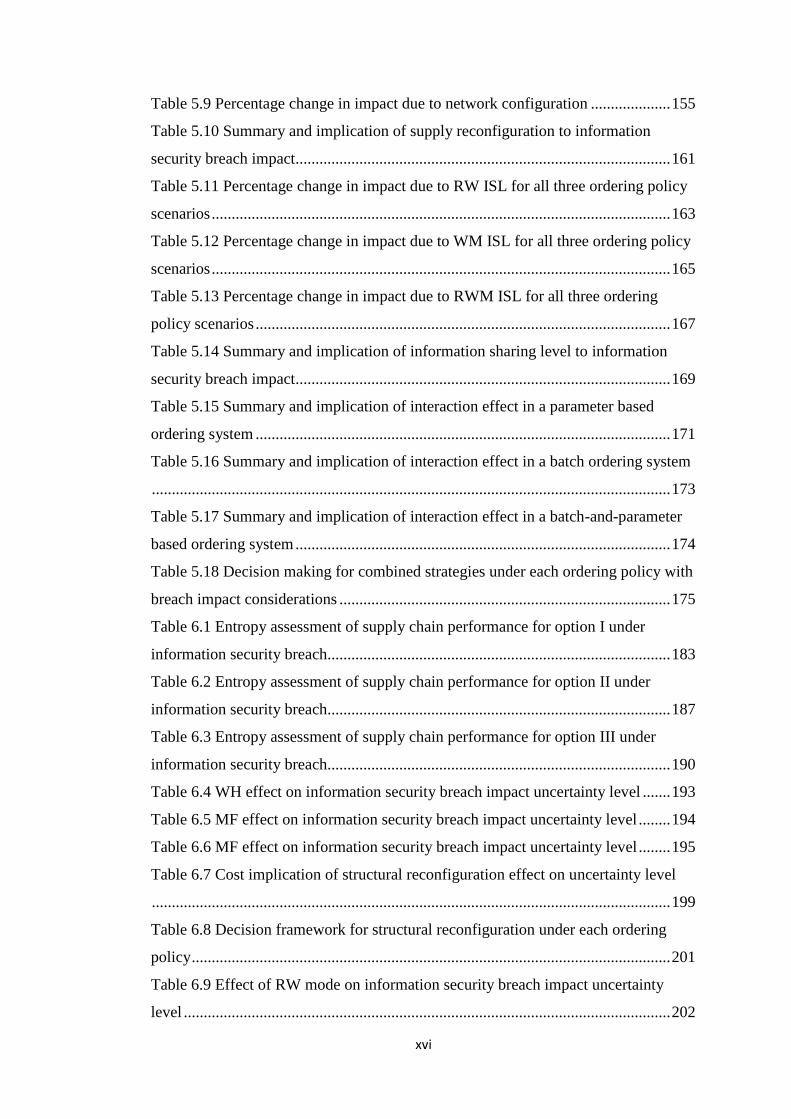
xvi

Table 5.9 Percentage change in impact due to network configuration .................... 155

Table 5.10 Summary and implication of supply reconfiguration to information

security breach impact.............................................................................................. 161

Table 5.11 Percentage change in impact due to RW ISL for all three ordering policy

scenarios ................................................................................................................... 163

Table 5.12 Percentage change in impact due to WM ISL for all three ordering policy

scenarios ................................................................................................................... 165

Table 5.13 Percentage change in impact due to RWM ISL for all three ordering

policy scenarios ........................................................................................................ 167

Table 5.14 Summary and implication of information sharing level to information

security breach impact.............................................................................................. 169

Table 5.15 Summary and implication of interaction effect in a parameter based

ordering system ........................................................................................................ 171

Table 5.16 Summary and implication of interaction effect in a batch ordering system

.................................................................................................................................. 173

Table 5.17 Summary and implication of interaction effect in a batch-and-parameter

based ordering system .............................................................................................. 174

Table 5.18 Decision making for combined strategies under each ordering policy with

breach impact considerations ................................................................................... 175

Table 6.1 Entropy assessment of supply chain performance for option I under

information security breach...................................................................................... 183

Table 6.2 Entropy assessment of supply chain performance for option II under


Table 6.3 Entropy assessment of supply chain performance for option III under


Table 6.4 WH effect on information security breach impact uncertainty level ....... 193

Table 6.5 MF effect on information security breach impact uncertainty level ........ 194

Table 6.6 MF effect on information security breach impact uncertainty level ........ 195

Table 6.7 Cost implication of structural reconfiguration effect on uncertainty level

.................................................................................................................................. 199

Table 6.8 Decision framework for structural reconfiguration under each ordering

policy ........................................................................................................................ 201

Table 6.9 Effect of RW mode on information security breach impact uncertainty

level .......................................................................................................................... 202

xvii

Table 6.10 Effect of WM mode on information security breach impact uncertainty

level .......................................................................................................................... 204

Table 6.11 Effect of WM mode on information security breach impact uncertainty

level .......................................................................................................................... 205

Table 6.12 Cost implication of structural reconfiguration effect on monitoring and

review cost ............................................................................................................... 206

Table 6.13 Decision framework for ISL adoption under each ordering policy ....... 208

Table 6.14 Relative change in uncertainty level due to ISL and structure interaction

effect ......................................................................................................................... 210

Table 6.15 Cost implication of the interaction effect on monitoring and review cost

.................................................................................................................................. 211

Table 6.16 Overall Mitigation Benefit under combined strategies .......................... 212

Table 6.17 Structural reconfiguration strategy decision given various ISL............. 214

Table 6.18 Information sharing level strategy decision given various supply

structures .................................................................................................................. 214

Table 6.19 Decision making for combined ISL and structural reconfiguration

strategy ..................................................................................................................... 215

1

Chapter 1 INTRODUCTION

1.1BACKGROUND

Traditionally, Supply Chain Management (SCM) focused around the manufacturer

and their immediate suppliers. But in today’s world, SCM focuses on the

optimization of all movement of goods and/or services and the flow of information,

starting with the suppliers’ supplier all the way through to the customers’ customer

(Plenert, 2002). In other words, firms have seen the need to manage the physical

flows and the information flows up and down the supply stream in a coordinated

manner. Management of these flows are increasingly becoming more challenging as

there is currently a marked increase in the geographical dispersion of manufacturing

sites, suppliers, warehouses and customers in today’s supply networks (Colotla et al.,

2003). However, Information Technology (IT) has been effective in improving the

efficiency of inter-organizational operations by mitigating uncertainties inherent in

collaborative networks via efficient transmission of information. IT has been used

extensively by supply networks to enhance the efficiency and effectiveness of supply

operations. Beyond that, it has been used as a vehicle for both internal and external

integration. For most organizations IT is core to their competitive advantage.

According to Wiengarten et al (2010) information quality plays a pivotal role in the

success of collaborative practices, and this is due to quality factors such as

timeliness, accuracy, relevance and added value of the shared information. It is safe

to say that most organizations are now extending the way IT is being utilized to

improve their competitiveness in this highly competitive global market. For example

the concept of cloud computing is a somewhat recent development in the way IT is

being exploited where hardware or software resources, or a combination of both, are

accessed anywhere in the world by an organization or an individual via the internet

(Amir, 2009, Smith, 2009, Armbrust et al., 2010). These resources are shared

amongst many users, abstracted, available on demand, scalable, and configurable

(Marston et al. , 2011). Some have even extended the concept to manufacturing

where product design, manufacturing, testing, management, and all other stages of a

product life cycle are encapsulated into cloud services and managed centrally (Xu,

2012) similar in principle to (but not the same as) distributed manufacturing

described in Dekkers and Bennett (2009). Essentially the idea is to pay for what you

2

use as opposed to renting where you pay for the specified period irrespective of use

(Subashini and Kavitha, 2011), which can be quite expensive. These growing

advantages of leveraging processes using IT and the fact that IT cost is becoming

more and more inexpensive have led to the increasing level of collaboration found in

many networks.

There is an increase in the level of connectivity and interdependency (referred to as

complexity) found in the network as businesses come together in the spirit of

collaboration being geographically distant from one another. These complexities

affect the dynamics of the network and thus require an appropriate network

management approach. It is perceptible that as complexity increases so does the level

of uncertainty enveloping the business or supply chain. A compromise in the

operations of one member could affect other interconnected members of the network,

the extent to which depends on how reliant their operations are on the compromised

company (Craighead et al., 2007). It is therefore apparent that strategies should

change to accommodate the increased or increasing complexity present in the supply

chain. Consequently there should be a pro rata increase in the level of information

required to monitor and control the operations of the network.

Nowadays it is difficult to separate information from operation as the absence of

information results in the poor performance of supply operations. Managing supply

operations effectively requires efficient management and use of information. One

cannot be managed with total disregard to the other, it will only spell disaster. The

fusion of both is crucial to business survival and serves as the foundation for

competitive advantage. This study is positioned to examine an aspect of supply chain

management which is information management by looking at the disruption in the

flow of information and how this affects supply chain management practices. It will

be interesting to know which areas of operation are most vulnerable.

1.2 NEED FOR INFORMATION SECURITY MANAGEMENT

As information is shared with the aid of Information Technologies (IT) and

Information Systems (IS), practitioners, therefore, are expected to increase their

effort in protecting their systems to reduce their vulnerability to system failure.

However, security controls appear to be lagging behind the use of new technology

(Baker et al., 2010, Potter and Beard, 2012). This is due in part to the fact that the

3

number of occurrence of these incidents is quite small and very unpredictable,

therefore most practitioners are not motivated to plan against them as planning incurs

a huge cost. Besides this, most organizations are not even prepared to restore their

services after disruption from information security breach1 and are unable to manage

other consequential impacts on the organization. It is therefore necessary for each

organization to assess the impact of security incidences on business operations,

regardless of whether they have never experienced it before, and how this affects

other businesses linked to it. This assessment should reveal ‘where?’, ‘what?’ and

‘how?’ business is affected and this in turn would provide the necessary incentive

that will encourage managers to proactively plan for any future occurrence. Pre-

empting disruption and planning for and against it has been shown by Mitroff and

Alpaslan (2003) to be beneficial to firms as proactive businesses existed for an

average of sixteen years more than their reactive counterparts. Unfortunately

businesses are still not taking this issue as seriously as they should. According to

Mitroff and Alpaslan (2003) and Altay and Ramirez (2010), 95 percent of Fortune

500 companies are unlikely to be able to manage a disruption that the company has

not experienced before because they are unprepared. There is therefore the need to

profile different information security breach types (also called threats2) in order to

understand the level of impact each has on an organization or supply chain as no two

threats are exactly the same and they differ in the magnitude of impact each has on a

business and supply chain.

As threats to information security take various forms, their incidence could reduce

the quality of information or even prevent accessibility to information. These

incidences may result in delayed transmission of information which might reduce the

relevance or value of the information, or altogether jeopardize the accuracy of the

shared information. Depending on the form of threat, they can cause systems to crash

preventing suppliers and other Supply chain members from having access to the

service, hence disrupting the flow of transactions leading to loss of money amongst

1 The incidence of an information security threat compromising the integrity, confidentiality or

availability of information needed for daily operations

2 An event or action that can potentially inflict harm or damage to the functioning of an IT system

4

other intangible yet crucial losses. A classic example is the 2011 breach incidence in

Sony’s PlayStation Network (PSN) which resulted in unavailability of service for

weeks and cost the business billions of dollars (Osawa, 2011).

1.3 NEED FOR APPROPRIATE SUPPLY CHAIN MANAGEMENT

STRATEGY

Organizations now understand the value of information and the need to protect their

information from outsiders with malicious intent or from competitors to maintain the

competitive advantage they have by leveraging such information. By examining the

impact of each threat, one can lay a foundation upon which appropriate supply chain

decisions are made. It is important to understand what level of integration (or

information sharing) in the supply chain is appropriate considering the impact these

threats have and how it affects performance of the entire network. Equally important

is the way the entire network can be reconfigured to increase its resilience to threat

impact outside of information security management efforts. For example which

ordering policy would reduce the impact of information security breach on the

supply chain performance more and how does impact at one tier in the supply chain

affect the entire network? Also how are the different supply structures affected by

these threat impacts. Beyond this, management should concern themselves with the

areas of operation that requires the most attention depending on their vulnerability.

Combining the answers to these questions would help create a better understanding

of the dynamics of the supply chain and the interaction between information

management and operations management. This would inform an appropriate strategy

designed to cater for the needs of specific collaborative networks. This study stems

from the need to develop concepts suitably adapted to supply chain management

which is different from those intended for individual organizations. Understanding

some of the dynamics mentioned earlier provides valuable insight and is a positive

step in the right direction.

1.4 PROBLEM STATEMENT

Threats to the security of an IT system are becoming increasingly sophisticated and

may result into loss of integrity, disruption of service and/or loss of confidentiality.

Therefore the security risk of any Information System (IS) should be assessed and

the appropriate countermeasures at the right level should be implemented. There are

5

many studies on the financial impact of threats to an organization, and a few have

studied the distribution of risk to supply chain members. However there is yet to be

found, a study in literature that has investigated the impact of information security

breach on the performance of the supply chain at both operational (supply chain

agent level) and strategic level (supply chain as a whole). Studies which have

investigated the impact of security breaches have been largely qualitative and

confined to individual organizations. These studies are quite subjective and lack

consistency. There is need for an objective assessment which a quantitative study

offers. This study will fill this important gap by conducting a quantitative assessment

of the impact of information security breach and provide knowledge on how the

incidence of these threats affects the operations of the supply chain. To prevent any

obfuscation of terms, some of the key terms used in this study are defined in Table

1.1.

Term Definition

Threat An information security related event or action that can

potentially inflict harm or damage to the functioning of an IT

system

Breach The incidence of a threat or the onset of an attack.

Information

Security Breach

The incidence of an IT related threat compromising the

integrity, confidentiality or availability of information needed

for daily operations

Risk The chance of a threat occurring (in this case Information

security breach) having either a negative or positive impact on a

firm or supply chain

Uncertainty Refers to the unpredictability of the what future impact would

be whether positive or negative or what the extent of negative

impact will be

Supply Structure The configuration of the supply chain that indicates the number

of agents in each tier of the supply chain

Entropy A measure of the amount of uncertainty associated with

predicting future impact of a specific breach under varying

supply context.

Ordering pattern This is defined as the combination of the average effective order

quantity and the frequency of placing an order

Table 1.1 Definition of key terms

In assessing risk, in this case threats to information security, the impact of the

incidence of such threat should first be estimated. It is apparent from literature that

this estimation has not been sufficiently covered as it is not understood how an

attack in one business will affect other aspects of the supply chain. This is called the

6

reverberating effect. Putting this in a supply chain context, it is not yet evidenced

whether this will have a ripple effect (similar in principle to the bull-whip effect

where there is significant increase in impact) or a trickle-down effect (i.e. where

there is not a significant increase in impact) on members as one goes upstream the

supply chain. Several questions arise from past studies which beg for answers. For

example how does security breach affect each member of the supply chain, and what

effect does it have on the entire chain? What effect does the structure of the supply

chain have on how security breach impacts supply chain performance? What effect

does the level of integration of the supply chain have on how security breach impacts

supply chain performance? How does the ordering decision mitigate or exacerbates

the impact that information security breach has on supply chain performance? The

formal research questions of this thesis will be formulated in the next section.

1.5 OBJECTIVE AND SCOPE OF RESEARCH

1.5.1 Strategic Factors Considered in the Study

Four structures are considered namely: serial, wholesaler type (WH), manufacturer

type (MF) and network type (NT). These are properly defined in the methodology

section. The WH and MF structures are considered to be structural reconfiguration

strategies which entail a unification and simplification of two separate serial

structures where there is only one agent in the wholesaler and manufacturer tiers

respectively while the NT structure is considered a risk pooling strategy where each

tier aggregates demand from downstream and shares it equally amongst themselves.

To study the effect of integration, information sharing (also termed information

integration) is conceptualised in this study as an upstream agent privy to the demand

and other related inventory information of a downstream agent. Examples of the

information being shared are inventory position, safety factor, lead time, ordering

cost, backlog cost and holding cost. Four levels of information integration are

considered: no integration (NI); integration between the retailer and wholesaler

(RW); integration between the wholesaler and manufacturer only (WM); and

integration between all three agents (RWM). RW and WM are partial forms of

information integration existing between different agents.

Three ordering policies are examined based on the ‘how much to order’ decision.

The first ordering policy considered is the parameter based ordering system where

7

the decision on how much is being ordered to the upstream agent is determined by

the difference or addition of two or more decision parameters. The second ordering

policy is called the batch or fixed ordering system where the order quantity has a

somewhat fixed value. The third one considered in this study is the combined batch-

and-parameter based ordering system where the order size is determined by a

combination of fixed order quantity and a parameter based order quantity. These are

fully explained in the literature review (Chapter 2) and methodology (Chapter 3).

1.5.2 Research Questions

The combination of the supply structure or configuration, the ordering policy and the

level of information sharing may be different for various supply chains and this

brings about varying levels of complexity. Complexity is mostly construed to mean

the configuration of physical asset, material flow and operational characteristic or

property of the supply chain which makes operations difficult to manage effectively

and efficiently (Serdarasan (2013) Wilding (1998)). In summary, it is the aim of this

research to provide insight on how these complexities affect the impact that various

information security breaches have on supply chain performance. To do this this

study is divided into three parts, Study 1, 2 and 3.

1.5.2.1 Study 1

The first study examines the influence of the interaction between these strategic

factors under normal circumstances (i.e. in a non-information security breach

scenario). Effectively the main question here is:

Question 1: How do these strategic factors interact and what influence do these

interactions have on supply chain performance?

Studying the effect of these three strategic factors in a single study has been missing

in literature and this study aims to fill that gap. Therefore the study examines the

interaction between these three factors and the effect of this interaction on supply

chain performance, which has not been studied extensively in the past. This

knowledge is important to build a better holistic understanding of the dynamics of

supply chain interactions. More to the point is that this study also serves as a

reference point for the next study which is understanding the impact of information

security breach and the role of these strategic factors in either mitigating or

exacerbating this impact.

8

1.5.2.2 Study 2

The second study builds on the first study to determine what the impact of

information security breach is on supply chain performance. However, while it is

important to understand the cost impact of these breaches, it is more so imperative to

establish which aspects of operation or areas in the supply chain are most vulnerable.

This will particularly help the supply chain prioritize ‘what?’ and ‘where?’ along the

supply chain require immediate protection and what appropriate mitigation solution

should be adopted on the long run. This way, the supply chain can effectively and

efficiently plan its operations, optimally prepared for any eventualities. To build this

understanding, the following questions are proposed and answered:

Question 2: Does the impact of information security breach increases or decreases

as one goes upstream?

Question 3: What is the effect of increasing the rate of occurrence (RoC) or

disruption duration of the breach from low to high on the impact a breach has on

supply chain performance?

Question 4: Are the improvement strategies beneficial to the supply chain especially

under disruption brought about by information security breach?

Beyond this, the study also aims to establish the role of these strategic factors in

either mitigating or exacerbating this impact. A mitigating role would indicate that

such strategic factor can be used to dampen the impact of a security breach when it

occurs and this can be a good addition to any proposed information security impact

management strategy.

1.5.2.3 Study 3

This research posits that the type of cost impact examined in study 2 represents a

direct cost assessment considered by most organisations which they use in decision

making. However this study opines that there exist an indirect cost implication that

also needs to be considered before making any strategic decision. The argument for

this approach stems from the fact that the estimated cost impact is quite uncertain in

itself and the complexity of the supply chain could exacerbate this uncertainty and

make it more difficult for supply chain managers to predict future impact. The ability

to predict future impact is a form of control that any manager would like to have as

this control is key to effective management. Therefore, a supply chain with high

impact uncertainty would require a higher monitoring and review control level

because of the high uncertainty associated with predicting future impact, while that

9

with low uncertainty would require low level of control. Increasing or decreasing the

monitoring and control level due to changing complexity has cost implications which

is regarded as an indirect cost. The question arises; how does supply chain

complexity affect the impact uncertainty level of an information security breach and

what implication does this cost have on supply chain strategy decisions? This type of

analysis has not been seen in past literature, at least to the author’s knowledge, and

this study aims to fill that gap. Finally, a decision framework is established that help

supply chain stakeholders make strategic decisions based on both direct and indirect

cost assessment.

1.5.3 Research Scope

The cost investigated by this study are operational costs, and do not include cost

associated with damage to company’s image or regulatory fines. The study

investigates the impact each security breach has on supply chain cost performance

such as inventory holding, backlog, and ordering costs only. It also examines the

effect on supply chain performance measures such as fill rate and the ordering

pattern of individual agents. While the holding cost, backlog cost, ordering cost and

fill rate are common performance measures used in past literature, the examination

of the ordering pattern is unique only to this study and is established in this study to

have implication to the transportation strategy used in the supply chain. Due to the

different complexities found in different supply chains, this study uses an analysis of

the ordering pattern to inform the appropriate transportation (or shipping) strategy.

By looking at the impact of these breaches on supply chain performance, including

the entropy assessment, one can begin to understand the dynamics of these security

incidences in order to plan for an effective prevention-mitigation-correction strategy

mix that suits the overall organization and supply chain management goal.

1.6 RESEARCH APPROACH AND FRAMEWORK

The framework for this study is shown in Figure 1.1. This is discussed in more

details in the methodology section.

To answer some of the questions stated above, this study proposes the use of discrete

event simulation (DES). DES is one of the three types of dynamic simulations that is

most widely used in Management Science (Pidd, 2003). This approach employs

computer simulation which makes it possible to mimic changes that occur, through

10

time, in real life systems by using model representation in order to understand,

change, manage and control such systems. The output of the simulation represents a

direct cost assessment of information security breach impact.

This study also utilizes the concept of entropy theory to measure the degree of

uncertainty or perturbation the incidence of each breach type (or threat) introduces to

the supply chain and its members and how this affects supply chain decisions.

Entropy according to Shannon (1948), who first coined the term in information

theory, is a quantitative measure of uncertainty. Entropy scores are calculated for

each threat (as will be explained in the Methodology section) and its implication to

monitoring and review cost is established. This represents an indirect cost

assessment.

Figure 1.1 Research Framework

1.7 STRUCTURE OF THE THESIS

This thesis is organized as follows.

Security Breach

Wholesaler

(WH)

Manufacturer

(MF)

Network

(NT)

Supply Chain Structure

Serial

(SS)

Backlog cost Ordering pattern

Ordering cost Fill rate

Inventory holding cost

Supply chain cost

Performance Strategic Operational

Level of Integration

Retailer +

Wholesaler

only (RW)

Wholesaler +

Manufacturer

only (WM)

Retailer + Wholesaler +

Manufacturer (RWM)

No

Integration

(NI)

Ordering Options

Batch based (option II) Parameter based

(option I)

Batch-and-Parameter

based (option III)

11

Chapter 2 reviews past works that forms the rationale for this study. It explains the

gaps in literature and offers a description of the strategic factors considered in the

study. The need for entropy assessment is also discussed.

Chapter 3 is the methodology part which describes the simulation approach. The

conceptual and computer models are discussed here along with the various computer

experiments. This chapter also describes the entropy assessment methodology which

is one of the significant contributions of the study.

Chapter 4 discusses the result of the simulation experiment under all non-breach

scenarios. The influence of each strategic factor is evaluated along with the

interaction effect of all three factors on supply chain performance.

Chapter 5 examines the impact of information security breach on supply chain

performance under various supply chain context. The effect of structural

reconfiguration and information sharing level on breach impact is evaluated both

separately and in combination. A framework for best strategy is given and the

rationale for stepwise adoption is established.

Chapter 6 reveals the result of the entropy assessment of information security breach

impact. The uncertainty level in each supply scenario is discussed and the effect of

structural reconfiguration and information sharing level in raising or decreasing the

uncertainty level is also discussed. The implication of uncertainty level change to

monitoring and review efforts and the cost consequence is debated. Finally, a

framework that justifies the inclusion of entropy assessment in supply chain breach

mitigation decisions is established.

Chapter 7 concludes and summarises the theoretical contribution of the study. The

managerial implication of the main findings is also discussed. Finally the limitations

of the study and recommendation for future work are given.

12

Chapter 2 LITERATURE REVIEW

Concerns over the efficiency and effectiveness of supply chain operations have been

raised over the years by academics as well as practitioners. These inefficiencies have

been perceived to be as a result of uncertainties in key aspect of operations, which

affect the flow of information and material along the supply chain. For example,

uncertainties in demand, supply and processes for a long time, have led to distortion

in the accurate capture of demand information and the ability to respond to them in a

timely and efficient fashion. Traditionally, due to the absence of the integration

initiative at the time, most members in each tier of the chain relied on historical

demand or order data to forecast future demand. The traditional forecasting method

could not accommodate the uncertainties of demand. As a result, supply chain

members had to order and produce surplus to be able to accommodate these

uncertainties. An interesting pattern emerged as the forecasted demand was

amplified the further you go upstream the chain (Lee et al., 2004). The consequence

of this action was that there tend to be more inventories in store than is needed,

which can be very costly and even worse if the products are perishable. These

uncertainties have led to poor performance of the supply chain and the reduction in

the quality of product and/or services offered.

2.1 SUPPLY CHAIN MANAGEMENT - FROM COMPETITION TO

COLLABORATION

Traditionally, Supply Chain Management (SCM) focused around the manufacturer

and their immediate suppliers, but in today’s world, SCM focuses on the

optimization of all movement of goods and/or services, starting with the suppliers’

supplier all the way through to the customers’ customer (Plenert, 2002). In other

words, firms have seen the need to manage the physical flows and the information

flows up and down the supply stream in a coordinated manner. Therefore

competition in the global market place has grown from inter firm competition to a

highly efficient collaborative supply chain network within and between industries

(Lancioni et al., 2003). Organisations no longer relate to suppliers in a competitive

manner and have adopted a collaborative approach where an organization aligns

itself or some of its business functions with those of its counterpart-suppliers. Suffice

to say, supply chain management has seen a paradigm shift from competition to

13

collaboration and this shift is premised on the need for improved efficiency and

effectiveness in the supply chain.

2.1.1 Managing Supply Chain Uncertainty through Information Sharing

It is quite apparent that the world is currently in the information age and

consequently business should be conducted with this in mind. A business would

thrive if it can position itself to leverage as much relevant information as possible.

Several studies have shown that supply chain performance can be improved, not only

by sharing demand information, but other types of information such as production;

inventory; capacity; and lead time information, as you go upstream (Mukhopadhyay

and Kekre, 2002, Kulp et al. , 2004, Devaraj et al., 2007, Yu et al., 2010, Lau et al.,

2004). This enabled supply chain members to keep just the amount of inventory

needed to efficiently cater for demand. The idea of information integration (in which

IT is used to leverage operational activities) emerged as the new paradigm. As these

IT technologies evolved, it later became apparent that it was not just enough to share

relevant information but that the information being shared should be of good quality

and be passed in a timely manner to help mitigate the effect of supply chain

uncertainties (Bourland et al. , 1996, Wiengarten et al. , 2010).

2.1.2 Business and the Information Integration Paradigm

Information Technology (IT) has been the tool used by organizations (large or small)

to greatly enhance their business operations via efficient information exchange.

Information technology especially has been extended to increase the amount of

benefits it can offer. For many years now technology has seen various developmental

phases and the benefits derivable from its use has driven its further development.

There have been massive improvements in the way organizations integrate business

functions (and or processes) internally and externally with other business partners

via electronic link. As described by Waters (2006), internal integration has been

improved by tracking individual packages using bar codes, magnetic stripes and

radio frequency identification (RFID) (Belal et al., 2008); monitoring vehicles

through telematics; controlling warehouses through automatically guided vehicles;

monitoring transactions and planning operations – and a host of other functions. In

the same vein, external integration has been extended by allowing vendor-managed

inventory (VMI); collaborative planning, forecasting and replenishment (CPFR);

14

synchronized material movement through the whole supply chain, payments by

electronic fund transfer (EFT), roadside detectors to monitor traffic conditions and

route vehicles around congestion – and so on. This integration, internal or external, is

premised on uninterrupted communication or information sharing.

Communication between businesses has greatly improved over the years with the use

of Information Systems (IS) such as Inter-organizational Information Systems (IOIS)

and huge efforts have been invested into communication with customers as well.

Fuelling this agenda is the plethora of investigations into the benefits of

communication and information sharing that can be found in literature (Bourland et

al., 1996, Chan and Chan, 2009, Cheng, 2010, Kristal et al., 2010, Li et al., 2006, Li

and Lin, 2006, Yang et al., 2011, Zhou and Benton Jr, 2007, Yu et al., 2001,

Raschke, 2010). Many researchers have looked into information sharing between

businesses and their customers (B2C) while others have examined it in terms of

business to business (B2B) (Mukhopadhyay and Kekre, 2002, Li et al., 2006,

Humphreys et al., 2001, Zhou and Benton Jr, 2007, Yu et al., 2001). However, from

the supply chain perspective information sharing is considered from both the B2B

and B2C point of view.

At a network or supply chain level, competiveness is no longer a case of sharing

information but how efficiently it can be transmitted. The development in

Information Technology (IT) seriously helped this course as the introduction of

Information systems such as Electronic Data Interchange (EDI); World Wide Web

(WWW); E-Commerce systems and especially the Internet has aided the timely

exchange of data (Gunasekaran and Ngai, 2004). This not only helped mitigate the

effect of supply chain uncertainties but enabled intra-organization information

sharing as well as inter-organization transactions (Kappelman and Richards, 1995).

2.2 GROWING USE OF THE INTERNET

According to some experts, complexity of the supply chain is increasing, profoundly

fuelled by the growing level of internet use and integration initiatives, as evidenced

by the number of networks current IT systems are supporting (Yami et al. 2010).

Due to its ubiquitous nature, the internet is being employed in multidimensional and

multifaceted ways in various supply chains to improve the quality of information and

integration initiatives. Irrespective of the type of supply chain, the internet has

15

proven to be limitless in the purpose it can serve provided its use had been carefully

or strategically planned. Its use has ranged from communication information

exchange (Hart et al. , 2000) to more operational related functions such as order

filling, purchasing, human resource management etc. (Lancioni et al. , 2003). These

systems are increasing in the level of support and function provided and the cost of

their application is increasingly becoming inexpensive where many small and

medium size enterprises can now afford technologies that were beyond their reach

due to lack of affordability. An example of this is the concept of cloud computing

which is a somewhat recent development in the way IT is being exploited. It is a way

of accessing hardware or software resources, or a combination of both, anywhere in

the world by an organization or an individual via the internet.

2.2.1 Cloud Computing- Internet Use Example

At the most basic definition, cloud computing entails using computing resources

such as computer applications and programmes over the internet as opposed to

license-and-install on the desktop (Buttell, 2010). Leveraging Information

Technology (IT) can be costly and has deterred small to medium scale organizations

from using it. This in part has led to the emergence and justification for the

somewhat new IT concept called ‘cloud computing’. The emerging trend of enabling

IT systems on the platform of cloud computing has been a subject of discussion in

recent years. A purely functional definition of cloud computing is that it is a way of

accessing hardware or software resources, or a combination of both, anywhere in the

world by an organization or an individual via the internet (Amir, 2009, Smith, 2009,

Armbrust et al. , 2010). These resources are shared amongst many users, abstracted,

available on demand, scalable, and configurable (Marston et al. , 2011). Although

this is not an entirely new concept, its unique feature where resources are pulled as

opposed to being pushed makes it a more promising concept than its predecessors;

time sharing in the 1960s and application hosting in the 1980s (Amir, 2009,

Cusumano, 2010). Its applicability would entail seeing this concept being delivered

over different service configurations. There are three basic service configurations

also known as cloud service models which are Software as a Service (SaaS),

Platform as a Service (PaaS) and Infrastructure as a Service (IaaS). In SaaS, the

cloud user buys the right to use a working application hosted by an external provider

via the internet. The PaaS model involves the use of an externally provided

16

infrastructure to host the application, while IaaS model requires the use of servers

provided externally for raw computing, storage and network transfers (Durkee, 2010,

Subashini and Kavitha, 2011). One can also look at the scope of the service whether

it is purely open to the public (Public Cloud) or restricted to certain users (Private

Cloud) or a combination of both (Hybrid Cloud).

2.2.2 Benefit of Cloud Computing

The result of an information security survey by Ernst & Young (2011) reveal close to

half of the total number of respondents from 56 countries have either deployed or are

evaluating cloud computing. This suggests that a significant amount of organisations

are now using or close to adopting cloud computing which in a way puts pressure on

others to follow suit. A summary of the opportunities organisations can avail

themselves to when they enable their IT on the cloud and the various concerns

associated with this new concept is shown in Table 2.1.

Cloud computing has several benefits over traditional IT models reported in

literature. Cloud services bring flexibility, configurability, cost effectiveness, low

implementation cost to IT and SCM. Primarily it offers a cost advantage to firms

especially the small to medium scale enterprises who otherwise cannot afford the

huge financial commitment required for deploying typical cutting edge enterprise-

level IT systems such as Enterprise Resource Planning (ERP) systems (Marston et

al., 2011). This is achieved through the metering system based on the notion of “pay

as you go”. Other benefits include taking away the associated costs of IT such as;

system upgrades; recruiting and training IT staff; equipment delivery and

installation; or modification of IT facility, from the Cloud user (Smith, 2009). It also

helps to prevent the loss that would otherwise be incurred when an organization is

unsuccessful in deploying an expensive in-house information system (IS). This is

because its flexible feature makes it possible to change from one cloud service

provider to another without any major cost to the user. If a service provider does not

deliver an agreed level of quality of service (QoS), the service user may change to

another provider offering a better or even cheaper service. These advantageous

features of Cloud computing can help organizations or supply chains to be lean, agile

or both (le-agile), responding effectively to demand. However there are some

concerns over its adoption with data security being the chief of those concerns.

17

Propellants for Adoption Barriers to Adoption

Elasticity/scalability: the

ability to scale IT infrastructure

requirements both up and down

rapidly

Corporate culture shock: going from internal

provision to external provision

Flexibility: ability to purchase

software components from

oracle, Apple, SAP etc and

combine it to form a business

solution

Quick provisioning: being able to scale

computing resources up or down at the level of

automation

Pay-as-you-go: pay-per-use

basis versus install-and-own.

Loss of control: managing IT infrastructure

through service level agreements (SLAs) with

Cloud Service Providers (CSPs)

Cost savings: reduction in IT

operational cost

Information security: How safe is your

information and data from security threats?

Stepwise adoption: ability to

decompose an entire technology

into piecemeal sizes and

gradually adopt it in stages

Privacy concerns: safeguarding personally

identifiable information of employees, business

partners and customers and meeting legal and

ethical requirements regarding privacy regulations

Infrastructure utilization:

virtualization of hardware and

software resources as a service

to multiple users simultaneously

Regulatory compliance: conforming to the

regulations of the part of the world where

hardware and software is located

Reducing market barrier:

reduction of IT barriers to

market entry. IT that was

unaffordable before can now be

utilised over the cloud.

Specificity: has to do with compatibility issues

and data lock-in.

Security: delivering “security as

a service”

Lack of standards: lack of commonality in

interoperability among cloud providers and

between enterprise systems and cloud services

Table 2.1 The opportunities and threats to cloud computing adoption

2.3 MANAGING INFORMATION FLOW DISRUPTION

It is very evident that nowadays, the flow of information is crucial to business

survival. For materials to move down the supply chain there has to be a prior

18

movement of information up the chain. A disruption in this flow of information

would have an effect on the movement of materials down the chain and hence lead to

customer dissatisfaction. It is not surprising that a study by Munoz and Clements

(2008) suggested that information flow delays play a larger role as a contributor to

lost sale revenues in the supply chain than material delay does. There is of course a

pressing need for operations managers to carefully protect and manage the flow of

information and plan appropriately for disruption in this flow. It stands to reason

therefore that while IT has been effective in curbing the effect of supply chain

uncertainties; IT (in itself) introduces inherent uncertainties to the supply chain.

Traditionally, the focus has been primarily on the uncertainties enveloping the

supply chain. However there is an increasing awareness of the unique uncertainties

that IT introduces to supply chain operations in the form of security risks. These

unique uncertainties represent the possibility of an incidence of threat which might

compromise the functioning of information systems (IS) and interrupt operations

leveraged by such systems. The security of any IS is pertinent to obtaining the

purported benefits derivable from its use. A secure system implies that there is no

possibility of disruption in operations with which the system is being used to

leverage. However, in practice, no system is totally secure as every system is

susceptible to breach.

Threats to the security of an IT system are becoming increasingly sophisticated and

may result in loss of integrity, disruption of service and/or loss of confidentiality

(Stoneburner et al. , 2002). Nonetheless, security controls appear to be lagging

behind the use of new technology (Baker et al., 2010, Potter and Beard, 2012). As

security breach comes in various forms, the quality of information or even the

accessibility to information can be compromised. This may result in delayed

transmission which might reduce the relevance or value of the information, or

altogether jeopardize the accuracy of the shared information. Therefore appropriate

countermeasures should be implemented. However, various countermeasures which

protect information systems from threats exist in practice, some more expensive than

others. As a result, organizations engage in risk management, which informs their

choice and level of countermeasure based on an assessment of risk incidence and

cost impact.

19

2.3.1 Types of Information Security Breach

According to Vinod et al. (2008), ISO27001 mandates that the potential threats to the

system and assets be identified in compliance with control A.7.1.1 (inventory of

assets), and this can be done by using an appropriate threat database. Several

databases exist that contain data on information security breach collected from

various organisations in the form of surveys. A survey done by

PricewaterhouseCoopers in conjunction with Infosecurity Europe, under the auspices

of the Department for Business Innovation and Skills (BIS), called The Information

Security Breach Survey (ISBS) 2012 reported some security breaches experienced

by various organizations. These include: Systems failure or data corruption;

Infection by viruses or malicious software; Theft or fraud involving computers; other

incidents caused by staff; attacks by unauthorised outsider including hacking

attempts (Potter and Beard, 2012). These breaches can be grouped under internal-

based, external-based or platform-based. The internal based security breaches are

those resulting from deliberate or in deliberate actions of staff and members of the

organization. External –based breaches include those perpetrated by outsiders who

are not members or staff of the business. This security breach can be worm; virus or

malicious software attack. It can also be password sniffing/cracking software;

spoofing (either IP spoofing or web spoofing) attack, denial of service attack (email

bomb attack or Ping O’Death), or direct attack (hacking) (Warren, 2000). Lastly the

Platform-based incidences are caused by the service provider. Examples of this

include; systems failure or data corruption resulting from poor resource management

or over committing computing resources (Durkee, 2010), policy violations or

physical damage or theft of the resources.

A survey done by Verizon Risk team joined by United States Secret Service (USSS)

also revealed some breaches faced by organizations and reported that 70% of data

breach was caused by external agents, 48% by insiders and 11% implicated business

partners (Baker et al. , 2010). Whitman (2003) proposed 12 categories of security

threat, namely: Act of Human Error or Failure (accidents, employee mistakes);

Compromises to Intellectual Property (piracy, copyright infringement); Deliberate

Acts of Espionage or Trespass (unauthorized access and/or data collection);

Deliberate Acts of Information Extortion (blackmail of information disclosure);

Deliberate Acts of Sabotage or Vandalism (destruction of systems or information);

20

Deliberate Acts of Theft (illegal confiscation of equipment or information);

Deliberate Software Attacks (viruses, worms, macros, denial of service); Forces of

Nature (fire, flood, earthquake, lightning); Quality of Service Deviations from

Service Providers (power and WAN service issues); Technical Hardware Failures or

Errors (equipment failure); Technical Software Failures or Errors (bugs, code

problems, unknown loopholes); Technological Obsolescence (antiquated or outdated

technologies).

These forms of security breach cause disruption in business processes and may

ultimately lead to loss of business. They can cause systems to crash preventing

suppliers and other Supply Chain members from having access to the service, hence

disrupting the flow of transactions leading to loss of money amongst other intangible

yet crucial losses. Depending on the form of attack, the magnitude of the impact of

such failure can be colossal and highly detrimental to Supply Chain performance.

2.3.2 Consequence of Information Security Breach

Security concerns as it relates to information sharing are privacy, protection of

proprietary information, and preservation of the quality of information. According to

Wiengarten et al. (2010) information quality plays a pivotal role in the success of

collaborative practices, and this is due to quality factors such as timeliness, accuracy,

relevance and added value of the shared information. Rees et al. (2011) described

three types of losses an organszation faces when they experience data breach:

damage to a company’s image, regulatory fines e.g. fines paid to Health Insurance

Portability and Accountability Act (HIPAA) due to non-compliance to regulation,

and production losses as a result of disruption in production’s IT support. The

National Institute of Standards and Technology in their 2002 report described three

types of impact on IT systems: loss of integrity, loss of availability and loss of

confidentiality (Stoneburner et al. , 2002). This paper aims to investigate the impact

of loss of availability or disruption due to security breach on the performance of

business operations.

2.3.3 Use and Reliability of Information Security Breach Survey Data

There have been several arguments as to the reliability of quantitative data on

security. Some have argued that most organisations that have taken part in surveys

cannot themselves attest to the fact that the information provided is near perfect.

21

Some have been heard saying they just had to put down a rough estimate (Rees et al.,

2011). Adding to this is the fact that incidence of security breach changes from year

to year some worse than others. It is believed that many security breaches go

unnoticed perhaps due to a poor monitoring system or the absence of it.

Corroborating this assumption is a survey by Baker et al. (2010) which revealed that

61% of data breach was detected by external parties. Organisations therefore need to

adopt a proactive approach rather than a reactive one to managing security. An

organisation needs to be able to detect any incidence of security breach within its

premises and must be able to log it. The ability to profile these breaches and

recognize ‘hot spots’, as these changes yearly, is paramount in establishing a

formidable security policy. Due to the rising level of sophistication hackers and other

fraudulent agents carry out their attacks, what might seem less harmful to an

organisation a few years ago might become the bane of existence.

Besides profiling the occurrence of breaches within an organization and learning

from one’s failure, it is equally important to learn from the failure of others. This is

why surveys are important so that one can make decisions not just based on one’s

internal data but on the likelihood that external data represents. According to Mitroff

and Alpaslan (2003) in Altay and Ramirez (2010), 95 percent of Fortune 500

companies are unlikely to be able to manage a disruption that the company has not

experienced before because they are ill-equipped. This is because many

organisations are not proactive towards information security breach and are quite

complacent towards a breach type that occurred in another organisation but not

theirs. However, according to a survey by Mitroff and Alpaslan (2003), proactive

businesses existed for an average 16years more than their reactive counterpart. This

goes to show that organisations need to learn from the failure of others and put

appropriate security measures in place to avoid being caught unprepared. Many

organisations are now using multiple sources in evaluating security threats (Potter

and Beard 2012). Although sometimes they may be restricted in terms of reliability,

security surveys give a good picture of the types of security threats faced by

organizations from different industrial sectors, a careful analysis of these data might

give invaluable insights. This is valuable information and should not be disregarded

on the account of reliability. Giving credence to this, the United States Secret

Service pooled resources together with Verizon Risk Team to come up with an

22

investigative report on data breach in 2009. Similarly, PriceWaterHouseCoopers in

conjunction with Info Security Europe, under the auspices of the Department for

Business, Innovation and Skills (BIS), conducted an information security breach

survey in 2010, although this has been organized in the past by BIS and its

predecessors (DTI and BERR) every couple of years since the early 1990s. There

are other surveys that aim to provide a rich pool of data on security breach.

Organizations need to realize the importance of other sources of information security

practices and incidents other than their own.

A study by Gordon et al. (2003) revealed that sharing security information with

partners helps to reduce the amount each firm spends on information security

activities. The view that no quantitative analysis should be done due to the

unreliability of security data, as it can change from year to year, has been suggested

by Rees et al. (2011) to be a minority view.

2.3.4 Risk Management

Threats to information security bring an organization to the possibility that their

operations would be disrupted and their data compromised. This possibility, also

referred to as risk probability, is defined as the probability of incidence of a threat

and is different for each threat (Kaplan and Garrick, 1981). In this study risk is

defined as the likelihood of a threat occurring (in this case Information security

breach) having either a negative or positive impact (Gerber and von Solms, 2005) on

a firm or supply chain. For the purpose of clarity, throughout this study, risk is

contextualized as the chance that a particular IT-related breach will occur and

compromise the security of information which in turn impacts the performance of an

organization in a negative way. Each breach is conceptualized as an incidence of

each form of threat and represents different risks to an organization. Examples of

these are systems failure or data corruption; infection by viruses or malicious

software; theft or fraud involving computers; other incidents caused by staff; attacks

by unauthorised outsider (including hacking attempts) etc. (Potter and Beard, 2012).

In risk management, all risks that the organization potentially faces are identified and

assessed, and the appropriate strategy is implemented to manage the incidence of

these threats (Stoneburner et al. , 2002). In coping with risks, organizations use all or

any combination of the following strategies: risk prevention and deterrence (also

23

called Prevention); risk detection and recovery (also called Mitigation), and risk

correction (also called Monitoring and Review) (Ouyang 2012). These strategies

involve management or administrative, operational and physical, technical or logical

tools. According to Ouyang (2012a), Management or Administrative tools include

policies; standards; processes; procedures; and guidelines. Operational and Physical

Control tools include execution of policies; standards & process; education and

awareness; program security; personnel security; document controls; facility or

infrastructure protection etc. Technical or Logical controls include, but are not

limited to, access controls; identification and authorization; confidentiality; integrity;

availability; non-repudiation.

According to Ouyang (2012), risk prevention deals with protective measures put in

place to prevent the occurrence of breach or deter perpetrators from attacking. This is

perhaps the first line of defense. An example of this is installing firewall or security

software. However this might not be very effective as breaches do still occur. The

second strategy which is the mitigation strategy helps to reduce the impact of the

incidence of breach when it occurs. A mitigating strategy would entail repair of

damaged assets, initiatives to restore integrity and reputation after the incidence of

threat, and efforts to bring back lost customers. For instance, backing up data on

another system can help an organization retain accessibility to valuable data in the

event of a compromise to the current system. It is more or less a recovery

contingency plan to keep the business going or to restore the operations of the

business to full functionality after severe attack. Choosing one or any combination of

these response strategies requires an earlier assessment of the threats an organization

is exposed to in terms of occurrence and cost impact (Rees et al 2011). The cost

impact is determined a priori and this is poorly estimated as it reflects more direct

costs and less indirect costs. The indirect costs such as loss of control are hard to

estimate and most studies in literature tend to ignore this when estimating the impact

on a business.

2.3.4.1 Risk Assessment

Being proactive requires rigorous risk assessment. However there are some

limitations on the components of risk assessment. Reducing vulnerability to threats

require the implementation of appropriate risk strategy which is informed by

adequate risk assessment. To assess any risk, the probability of incidence (P) is

24

multiplied by the cost impact (I) on the organization if it occurs (Deane et al. 2009,

Rees et al. 2011). These two components of risk assessment, P and I, have

limitations as estimating P is very difficult due to unpredictability3 and estimating I

is also very poorly understood. The inconsistencies in P and I result in poor

assessment of risks and could result into a Type-1 error or a Type-2 error (Banerjee

2009). A Type-1 error (false positive) occurs when an insignificant threat is poorly

assessed to be a significant one. Here, the organization wastes effort and resources

by implementing unnecessary risk management strategy where monitoring alone

would have sufficed. The Type-2 error (false negative) on the other hand occurs

when a significant threat is seen as an insignificant one. The effect of this is that a

less stringent strategy is implemented to manage the threat which would be

ineffective and result in an unprecedented impact on the organization. It stands to

reason that cost impact represents a higher interest to most organisations than the

probability of occurrence. It is logical that if the impact is high and despite the

probability of occurrence being very low, then such breach incidence is still a source

of concern for the organisation. If, however, the probability of occurrence is high and

the cost impact is low, then organisations may decide to forego the cost impact if it is

not too significant. Therefore the focus of this study is on the cost impact estimation.

2.3.4.2 Inconsistencies in Estimating Impact, I.

The threat-type incidence, hacking, experienced by Sony’s PlayStation Network

(PSN) in 2011 affecting up to 77 million consumers reportedly compromised over

ten million customer’s credit card information and was to cost the organization $171

million in remediation. This impact cost has been suggested by experts to be a rather

optimistic assessment and that the true impact might be in the region of billions of

dollars. Sony’s spokeswoman, Kumie Tanaka, was reported to admit that they could

not estimate the true impact of the breach at the time as they were still ‘figuring out’

the impact on its earnings (Osawa, 2011). Further to this, two different experts

Mizuho Investors Securities analyst, Nobuo Kurahashi, and Barclays Capital analyst,

Yuji Fujimori, reported an impact of $1.25 billion and $2.74 billion respectively

(Brightman, 2011). A difference of $1.49 billion in their estimates lends credence to

3 Refers to the changeable nature of the number of times threat incidence occur and the uncertainty of

whether or not it will occur.

25

the fact that Impact (I) is poorly understood, even by experts. An even bigger

estimate was reported by Forbes Business Magazine in tune of $24 billion impact

cost (Phillips, 2011). While it has been difficult to estimate the true impact cost on

an organization, it is even more difficult to estimate that for a supply chain. It is

therefore crucial to adequately assess each threat to determine the best strategy to

manage it. In literature, most IT breach impact studies are qualitative and are

restricted to an organizational level (Goel and Shawky, 2009). These qualitative risk

assessment studies are subjective and lack consistency. On the other hand, some

quantitative studies have looked at the impact of other types of threat (such as natural

disasters) to an organization, and some to the supply chain. However, there is no

quantitative study in literature that has investigated the impact of IT threat-type

incidences on supply chain material flow operations.

2.4 DISRUPTION RISK ASSESSMENT

A number of studies have approached disruption risk in different ways ranging from

conceptual, empirical, simulation, survey, case study and review or a combination of

these (Rao and Goldsby, 2009, Olson and Wu, 2010, Rainer et al., 1991). Rao and

Goldsby (2009) conducted an extensive review of supply chain disruption literature

and created a typology of disruption types and sources. However, they did not

mention IT itself as a source of disruption. Most risk studies have been primarily

based on threats other than those from IT and information communication

technologies (ICTs) while a few studies have suggested IT security as a potential risk

to the supply chain (Schmitt and Singh, 2009, Kim et al., 2011, Rees et al., 2011).

Table 2.2 shows a summary of work that has been done on disruption risk

assessment at the organizational level as well as the supply chain level and delineates

between those that have provided real and objective estimation of impact, I, of

certain threats on business operation and those that have looked at specific IT

security risks. The third column reveals the approach taken to undertake the study.

From the last three columns of the table we see that no single study has covered all

three aspects.

26

Authors Subject Approach Impact

study? Y/N

IT security

incident?

Y/N

Supply

chain study?

Y/N

Altay and

Ramirez, 2010

Impact of disasters on firms in different

sectors: implications for supply chains

Fixed effect regression Y N Y

Schmitt and

Singh, (2009)

Quantifying supply chain disruption risk Monte Carlo and Discrete-Event

Simulation

Y N Y

Deane et al.,

2009

Managing supply chain risk and disruption

from IT security incidents

Mixed Integer Linear Programming N Y Y

Munoz and

Clements, 2008

Disruptions in information flow: a revenue

costing supply chain dilemma

Discrete event simulation of beer

distribution game

Y N Y

Rees et al., 2010 Decision support for Cybersecurity risk

planning

Genetic algorithm N Y N

Whitman (2003) Profiling threats to information security Interviews and Survey N Y N

Wilson (2007) The impact of transportation disruptions on

supply chain performance

Dynamic simulation modelling Y N Y

Bellefeuille,

2005

Quantifying and Managing the Risk of

Information Security Breaches to the Supply

Chain

Descriptive research N Y Y

Yeh and Chang,

2007

Threats and countermeasures for information

system security: A cross-industry study

Questionnaires and Analysis of

covariances (ANCOVAs)

N Y N

Goel and

Shawky, 2009

Estimating the market impact of security

breach announcements on firm values

Event-study methodology Y N N

Craighead et al.,

2007

The Severity of Supply Chain Disruptions Multiple-method, multiple-source

empirical research design

N N Y

Kim et al., 2011 The dark side of the Internet: Attacks, costs

and responses

Explorative research N Y N

Loch et al., 1992 Threats to information systems: Today's

reality, yesterday's understanding

Questionnaires N Y N

Table 2.2 Summary of some relevant disruption risk studies

http://www.sciencedirect.com/science/article/pii/S1366554505000967?_alid=1818720069&_rdoc=2&_fmt=high&_origin=search&_docanchor=&_ct=19300&_zone=rslt_list_item&md5=61a9198f50af8b815fb9702c688b00aa

http://www.sciencedirect.com/science/article/pii/S1366554505000967?_alid=1818720069&_rdoc=2&_fmt=high&_origin=search&_docanchor=&_ct=19300&_zone=rslt_list_item&md5=61a9198f50af8b815fb9702c688b00aa

http://www.sciencedirect.com/science/article/pii/S0378720609000895?_alid=1818732613&_rdoc=3&_fmt=high&_origin=search&_docanchor=&_ct=366&_zone=rslt_list_item&md5=17a5cf3306b6b694e2dd22a43d0c0d28

http://www.sciencedirect.com/science/article/pii/S0378720609000895?_alid=1818732613&_rdoc=3&_fmt=high&_origin=search&_docanchor=&_ct=366&_zone=rslt_list_item&md5=17a5cf3306b6b694e2dd22a43d0c0d28

27

A few studies have examined the impact of disruption on supply chain operations.

While some of these studies have examined the effect of physical disruption such as

natural disasters (Samir, 2008), interestingly, a few others have examined the effect

of IT security incidents (Deane et al., 2009, Kim et al., 2011, Loch et al., 1992,

Pisello, 2004). Some approaches have focused primarily on disruption effects (in

terms of delay in information flow) on supply chain without any regard to cause

(Munoz and Clements, 2008, Schmitt and Singh, 2009) while others have looked

more specifically at how specific disruption types (threats) affect the supply chain

(Altay and Ramirez, 2010, Craighead et al., 2007). While the former approach gives

a more general assessment of the impact of disruption, the latter gives clearer

understanding of the dynamics of threats and how they impact the chain. From Altay

and Ramirez (2010) it is understood that disasters lead to disruption which affects all

sectors of the chain but certain threats have more impact than others. This type of

specific-threat impact study is not as common as one would expect in literature,

specifically in the area of information security management. It is still not quite

understood how the impact of various threats to information security on supply chain

performance vary (especially inventory management performance). Although a few

qualitative and quantitative studies (Whitman, 2003, Yeh and Chang, 2007,

Bellefeuille, 2005, Goel and Shawky, 2009) have looked at this in a rather subjective

way requiring managers to rank or score threats according to their perception, there

is still a lack of objective measure of these variances. Deane et al. (2009) examined

how risks originate from one business, due to poor countermeasures put in place to

prevent it, and is being transferred to adjoining firms in the supply chain using mixed

integer linear programming (MILP). While they termed the risks they studied IT

security incidents, there was no evidence of specific threats to security being

addressed and it is not clear how these risks affect the dynamics of the supply chain.

In a similar work by Rees et al. (2011), specific threats were addressed and the

financial impact for a given countermeasure was estimated. However, it was still

unclear how these threats affect the operations of an organization, not to mention the

supply chain. This threat-type impact study seems to be lacking in information

disruption literature. To know how these threats affect the performance of the

network is crucial to appropriate disruption risk planning and management.

28

Having reviewed literature, it was clear that there is a paucity of quantitative

research on information security as a potential source of disruption. Out of those that

have considered information security, a very few have tried to investigate how

threats to information security impact the supply chain: some purely qualitative,

others a mix of qualitative and quantitative. Of this few, none has investigated how

these affect the operations of the supply chain at an operational and strategic level

and how a breach in one organization affects others that are linked to it, although

they have not experienced any breach in themselves. For instance it is not yet

understood, in real terms, from these studies what the cost implications of security

breach in an organization’s procurement process are for supply partners. It is obvious

that these breaches can cause delays in transactions between supply chain partners

but it not well understood to what extent these delays will impact the operating cost

of members further upstream or further downstream of the supply network. There are

other key performance indicators that are affected such as ordering pattern which

may ultimately affect the shipping strategy of agents in the supply chain, but to what

scale are they affected? The understanding of how these impact not just an

organization but other members of the network is crucial to successful network

management or coordination activities. It has not been evidenced how the

complexity or conditions of the supply chain affect the impact of information

security breach on its operations.

Most security risk studies have been based on cost to an organization, and have

provided ways in which an organization can make economic assessment of

countermeasures available to them. While these studies have focused on direct costs,

there is yet to be a study that presents real evidence on indirect costs to the

organization. This indirect cost is discussed later in section 2.6.

2.5 MITIGATING ROLE OF SUPPLY CONDITIONS

The best solution to information security problems of course would be to have

appropriate levels of prevention and deterrence; detective and recovery, and

corrective measures (Ouyang 2012). Disruption duration is a function of the level of

security breach detection and recovery measures (otherwise called mitigation

measures). It is within reason that higher breach disruption duration means the

detection and recovery level is not high enough. Lower disruption duration is

29

indicative of having near appropriate level of detection and recovery measures. On

the other hand, rate of breach occurrence (RoC) is indicative of the required level of

security breach prevention and deterrence measures (otherwise called prevention

measures). Higher RoC means the preventive and deterrence measure is not at an

appropriate level, and lower RoC means that the level of breach prevention and

deterrence is high (Dai et al. 2012).

However, the incidence and type of security breach changes year in year out and as

such, businesses should be able to contain any changes using an appropriate security

management system that can analyse these changes (Potter and Beard 2012).

Breaches that were no longer an issue a year ago, being mitigated by the security

measures already put in place, might become a serious issue the next year rising

from changes in the incidence and level of sophistication with which these breaches

occur. In the same vein, breaches considered benign last year might become

malignant the next year following an increase in the number of occurrence.

Although many have reported that collaborative practices such as information

sharing are beneficial to the supply chain, others have shown that there are

moderating factors which affect these purported benefits. For instance, high cost of

making IT investment typical of bigger business ventures (Dermikan, 2010), quality

of information shared- timeliness; accuracy; relevance and added value (Weingarten

et al, 2010), mode of information sharing (Lau et al., 2002), contextual factors such

as external pressure and internal readiness of the organization, amongst other related

factors have been reported to undermine the benefits derivable from sharing

information. From this mix of studies, one can begin to appreciate the role of

preparedness and requisite understanding of one’s business environment (both

internal and external) in deriving the said benefits of any information sharing

strategy. It is therefore within reason, to assume that that the same information

security breach would impact supply chains in different ways due to the different

operating variables (also known as complexity drivers) found in various supply

chains.

2.5.1 Supply Chain Complexity Drivers

Several definitions of complexity exist in literature. Bozarth et al. (2009) defined

complexity as the level of detail complexity and dynamic complexity exhibited by

30

the products, processes and relationships comprising the supply chain. Serdarasan

(2013) defined it under static; dynamic; and decision making complexities.

According to Serdarasan (2013), Static complexity connotes the structure of the

supply chain, the variety of its components and strengths of interactions; dynamic

complexity describes the uncertainty in the supply chain which involves the aspects

of time and randomness; while decision making complexity involves aspects of static

and dynamic complexities. A review of complexity drivers was carried out in the

study of Serdarasan (2013) and the study listed various drivers which include, but

not limited to, number/variety of suppliers, number/variety of customers,

number/variety of interactions, conflicting policies, demand amplification,

differing/conflicting/non-synchronized decisions and actions, incompatible IT

systems. In a separate work by Hoole (2005), the study listed five complexity drivers

(which was referred to as performance levers); configuration; management practices;

external relationships; organisation; and systems. Wilding (1998) examined what he

called the supply chain complexity triangle: deterministic chaos, parallel interactions

and demand amplification. From these studies, it is very obvious that supply chain

structure, decision making policies (ordering policy), and the level of information

integration present in the supply chain are prominent common factors. Studying the

impact of an element in a supply chain setting should therefore include these three

variables and conversely, the influence of these three variables can be examined to

see how they affect the impact of the said element.

2.5.2 Conceptualisation of Supply Chain Structure

Supply chain structure or configuration has been suggested as one of the most

prominent performance lever that helps improve supply chain performance (Hoole,

2005). Configuration or structural complexity is mostly construed to mean physical

asset and material flow in the supply chain (Hoole, 2005); hence improving supply

chain configuration has been suggested as one of the most common methods for

reducing supply chain uncertainties and improving performance (Childerhouse and

Towill, 2003). Supply chain structure has been defined by many researchers based

on several parameters. Randall and Ulrich (2001) defined structure in their work as a

function of distance of production facility to target market and the extent of

production to reach minimum efficiency. In their work, Stock et al. (2000)

conceptualized structure as a function of geographic dispersion and channel

31

governance. Structure according to Xu et al. (2010) was defined in the context of

how the manufacturer directs its capabilities. They defined three structures; a

component supplier structure is one where the manufacturer produces components

for the original equipment manufacturer (OEM); a monopoly structure where the

manufacturer assembles the product under their own brand; and the dual distributor

structure which is a combination of the previous two. This study, however, adopts

the notion of structure found in Hoole (2005) based on the indication of what gets

done where?’. According to Hoole (2005), the Supply Chain Operations Reference

(SCOR); which is endorsed by more than 750 member organisations, breaks the

supply chain into four process elements (plan, source, make, deliver). These

elements are reflective of the role the retailer, distributor/wholesaler, and the

manufacturer/supplier play in the supply chain. It seemed quite appropriate to

include all these elements when defining a supply chain. Therefore structure in this

study is defined in terms of ‘how many agents are in each process element’, and the

retailer, wholesaler and manufacturer are all separate tiers in the supply chain. This

three tiered structure is more representative of a supply chain than a two tiered

supply chain, and on the other hand represents a simplified version of a four or more-

tiered supply chain.

Some studies have looked at the effect of supply chain structure on the performance

of supply chains (Beamon and Chen, 2001, Mills, 2004, Xu et al., 2010) but this has

mostly been an evaluation of the performance of one multi-agent structure to another

multi-agent structure. The performance of a simplified supply chain in the form of a

serial structure against two or more complex supply chain structures with multi-

agent components has not been studied, at least to the author’s knowledge. This type

of analysis is very important in complexity studies as simplifying the structure in

certain aspects may help reduce the uncertainties associated with such highly

complex supply systems. Beamon and Chen (2001) described four supply chain

structures based on a single manufacturer present in the chain namely; convergent

(assembly type), divergent (Arborescent type), conjoined (combination of

convergent and divergent) and general (also called network). They then examined

the performance of a conjoined supply chain structure while Lau et al. (2002)

included a linear structure (also called serial) in addition to what was described by

Beamon and Chen (2001) but they only considered the impact of information sharing

32

on a divergent supply chain in their study. It appears that many of these studies

consider various supply chain structures with one thing in common; there is only one

manufacturer in the chain, except for the network structure. In order to examine the

effect of structure on supply chain performance, this study evaluates the relative

performance of a distribution type, manufacturing type and network type structures

to a serial counterpart in disrupted and non-disrupted supply chain scenarios. In

addition the effect of structure on supply chain disruption has been under studied in

literature. Study of the structure effect in the context discussed above is one of the

contributions of this study.

2.5.3 The role of ordering options

Several studies have established the cost controlling effect of ordering policies in a

supply chain. These policies determine the key inventory decision of ‘when to order’

and ‘how much to order’. The ‘when to order’ decision is governed by certain

conditions that need to be met before an organisation can place an order to its

supplier. This could mean when the inventory position falls below a target level (re-

order point) after periodic or continuous checks (Axsäter and Juntti, 1997, Axsäter,

2003), or when an order is received from downstream agents in the form of

aggressive ordering (Papanagnou and Halikias, 2006) Agrawal et al 2009). The

condition mostly used in literature and in practice to decide if an order should be

placed is whether the inventory level falls below the predefined re-order point. This

point could generally mean a target level that must be kept at all times but may be

exceeded. The ‘how much to order’ can either be a predetermined quantity (batch

ordering) (Baganha and Cohen, 1998, Axsäter, 2003, Mitra and Chatterjee, 2004,

Tee and Rossetti, 2002) or the difference or addition between two or more decision

variables or parameters (Agrawal et al., 2009, Banerjee et al., 1996, Chen et al.,

2000, Chen and Disney, 2003, Wright and Yuan, 2008). The continuous review

model, (Q, R), and the order-up-to (OUT) comprising of the base stock model (r, S)

and the min-max (s, S) model, have been studied extensively. According to

Vasconcelos and Marques (2000), in the continuous review (Q,R) option, Q is

usually set to Economic Order Quantity (EOQ) and R is the re-order point computed

for each replenishment period. The EOQ model being deterministic usually fails and

causes a significant increase in cost when used in a stochastic environment. However

Axsäter (1996) proposed an optimal solution for Q by multiplying the EOQ by

33

square root of 1+α2 when α=2. This optimal model is used as one of the ordering

options in our simulation model. Another ordering policy commonly used in

research is the base stock option (r, S) where r represents the review period and S the

OUT level (Agrawal et al., 2009, Bensoussan et al., 2007, Beamon and Chen, 2001,

Chen et al., 2000). The other option is the OUT (s, S) option where s is the re-order

point and S is the order-up-to level (Chen and Disney, 2003, Lau et al., 2004, Arrow

et al., 1951). Again we see from several studies that organisations perform

differently under various ordering policies. In a study by Lau et al. (2008) they found

that the EOQ model held the most benefit for the retailer while the periodic order

quantity was more beneficial to the suppliers. However it is not evident from

literature how these policies perform under information security breach.

2.5.4 Role of Information Sharing

Information integration results in interdependencies amongst supply partners where

the upstream partners rely on key business information from downstream partners in

a timely manner. Therefore disruption in this flow of information could have a

negative effect on the movement of materials down the chain and hence lead to

customer dissatisfaction. Alluding to this reality is a study by Munoz and Clements

(2008) which suggests information flow delays play a larger role as a contributor to

lost sale revenues in the supply chain than material delay does.

Information sharing (or information integration as it is also called in this study) has

been a solution pushed by some research (Bourland et al. , 1996, Chan and Chan,

2009, Cheng, 2010, Kristal et al., 2010, Li et al. , 2006, Li and Lin, 2006, Yang et al.

, 2011, Zhou and Benton Jr, 2007, Yu et al., 2001, Raschke, 2010). A good amount

of research, both empirical and analytical, has been conducted in the area of

information sharing and how agents in the supply chain derive benefit from it, if any

at all. It has been reported that there exist benefit to members of the chain who

engage in information sharing especially those types of information that are

important to the timely operation of the chain such as demand, inventory, supply

lead time and capacity information (Mukhopadhyay and Kekre, 2002, Kulp et al. ,

2004, Devaraj et al., 2007, Yu et al., 2010). Although the benefit may be

disproportionately distributed amongst supply chain members (Yao and Dresner,

2008), each member strives to position themselves in a vantage point where benefit

34

accrues to them. The question has been who stands to gain the most if information is

shared, that is if there is any benefit to be derived at all. Therefore there has been

discussion about ways to incentivise members or agents in the chain that do not

directly benefit from information sharing (Yao et al., 2010).

2.5.5 The Need for a Systemic Study

There have been many studies looking at IS risks to an organization and a very few

have studied IS risk to the supply chain. However there is yet to be an academic

study on the impact of IS disruptions on the supply chain under various supply chain

context or conditions. The supply chain context is defined here as the state of the

chain in terms of the level of information sharing (information integration) present,

the specific ordering option being used and the structure of the supply chain. Table

2.3 reveals a list of some of the previous studies and the supply chain context their

work was based on. Three different contextual factors are considered in this study,

namely ordering option; supply structure; and information sharing level. Each

contextual factor or complexity driver has various alternatives. Under the ordering

option, Table2.3 shows three alternatives that have been studied which are parameter

based ordering (PBO); batch ordering (BO); and combined batch-and-parameter

based ordering (CBPO). The supply chain structure is examined whether it is a serial

type structure with only one agent in each tier of the supply chain or if there are

multiple agents (multi-agent) in each tier representing a more complex structure.

However the multi-agent type structure can also exist in different alternative forms

such as distributor, manufacturer, or network type structures. Under the information

sharing context, the table examined two alternatives, centralized and decentralized

information sharing, although the centralized option can also exist in two

alternatives: partial or full information sharing. It is clear that none have studied

supply chain contextual effect under all three categories together. Some have

examined the effect of these complexity drivers separately but there is a need to

build as much context as possible in supply chain studies. Perhaps a change in one

of these contextual variables in the supply chain may result in a completely different

outcome when the effect of the other two is examined. Also, it is not clear what the

interaction between the effects of two or more contextual factors is on supply chain

performance. In addition, it is not evident from literature how this contextual effect

35

Ordering Option Structure Information sharing

Author PBO BO CBPO Serial Multi-agent Centralised Decentralised

Papanagnou and Halikias (2006) * * *

Chen (1998) * * * *

Banerjee et al. (1996) * * * *

Agrawal et al. (2009) * * * *

Wright and Yuan (2008) * * *

Chen and Disney (2003) * * *

Hosoda and Disney (2004) * * *

Chen et al. (2000) * * * *

Sterman (1989) * * *

Wu and Edwin Cheng (2008) * * * *

Yu et al. (2001) * * * *

Lau et al 2002 * * * *

Lau et al 2004 * * * *

Chen and Samroengaja 2004 * * * *

Beamon and Chen * * * *

Chatfield et al. (2004) * * * *

Baganha and Cohen 1998 * * *

Table 2.3 Review of past contexual studies

36

or the interaction effect mitigates or worsens performance especially in an

information security breach scenario.

2.6 ENTROPY ASSESSMENT AND THE INDIRECT IMPACT COST

PARADIGM

While the direct cost impact of a security breach on two different

organisations/supply chains might be the same, the level of uncertainty associated

with such impact may not be the same due to the different complexities of both

organisations/ supply chains. In other words, the direct cost impact when the breach

occurs at another period in the same year might be different for both

organisations/supply chains. It is therefore necessary to capture this uncertainty and

this can be done using an entropy approach.

2.6.1 The Supply Chain Scenario Narrative

Consider a scenario where a supply chain contains the retailer, distributor,

manufacturer and supplier and it is known that information about demand flows from

the retailer through the chain to the manufacturer, which uses this information to

place orders to its supplier. Depending on the level of integration, supply partners

can access this information once they have access to the internet and plan their

operations effectively in a timely manner. Intuitively, one knows that if the system,

which the retailer uses in capturing demand, is compromised due to an attack that

makes service unavailable, the other parties in the supply chain would be denied the

advantage of knowing demand as it occurs or even denied access to real demand

information because the database has been corrupted. Consequently, they would

have to rely on forecasted demand in making ordering decision with their suppliers

and cannot take advantage of having timely demand information. Bourland et al.

(1996) revealed that a supplier could reduce inventories and its associated costs or

improve the reliability of deliveries to its customers given more accurate demand

information.

On the other hand if a system, with a customer interface, which allows a

customer to place an order to the retailer or manufacturer directly, becomes

unavailable due to security breach, or crashes due to a sudden increase in the number

of customers accessing the interface at the same time. The organization or supply

37

chain might lose that customer depending on the severity of the incidence. Severity

here means the duration of the breach and the number of repeated occurrences.

According to Hoffman and Lowitt (2008), retaining customers is critical to survival

of an organization, let alone growth. Assume, hypothetically, that a web service

where customers are able to place their orders online is compromised and has

become inaccessible to customers. This in effect will result in the customers

defecting to use services provided by competitors. The customers are classified into

two categories which are the ‘loyal customers’ (which are those accustomed to the

use the service and regularly patronize it) and the ‘likely customers’ (which are

trying the service for the first time and are looking for a reliable service to stick to).

From Capraro et al. (2003) and Hennig-Thurau and Klee (1997) it is understood that

loyal customers are still likely to purchase from vendors despite incessant

dissatisfaction. However, a research conducted by Accenture revealed that 70% of

US retail customers are loyal customers and that 85% of these “loyal” customers are

willing to shop elsewhere if properly enticed (Hoffman and Lowitt, 2008). In other

words, there is an 85% chance they could defect. Inaccessibility to service might be

the defecting factor which could cause ‘loyal customers’ to defect and ‘likely

customers’ to permanently defect. The breached organization would then have to

spend more money on promotional packages, among other things, to win back

customers.

The objective of any organization or supply chain would be to reduce the number of

occurrences of security breach or totally eradicate it if possible. It is understood from

the above that there is an 85% chance of losing customers or customer transaction if

they experience incessant dissatisfaction caused by security breach of the system. As

it has been established in section 2.3.4, one way of calculating the risk to an

organization is by multiplying the probability of incidence (P) of the breach by the

impact cost (I) incurred when that breach occurs (Rees et al., 2011, Deane et al.,

2009). Therefore, the higher the probability of an incident occurring the greater the

risk and vice versa. For instance if the cost incurred when an incidence occurs is

£20k and the probability of occurrence is 0.5, then the risk impact is £10k. If the

probability of occurrence reduces to 0.1 due to countermeasures put in place, then

the risk impact becomes less, £2k. In the same light, if there is an increase in the

probability of incidence then the risk impact increases. In essence once the cost

38

impact (I) is established, then all that requires monitoring is the probability of

incidence (P). Ideally any preventive measure would be to reduce the level of

occurrence of these breaches (i.e. P) and any mitigating measure would be to reduce

the impact cost (I). However there is still a conundrum yet un-tackled. The pre-

estimated impact cost is in itself uncertain. For example, the impact of a security

breach may vary depending on the time of the year it occurs. It is expected that the

same breach occurring during peak demand periods will have more cost impact than

when it occurs during the less busy periods of the year. Therefore this uncertainty

needs to be reflected in the risk calculations. A very well established means of

estimating uncertainty is the entropy theory which is discussed in the subsequent

section.

2.6.2 Entropy Assessment

Entropy has been described as a quantitative measure of uncertainty which describes

the level of chaos or surprise associated with an event (Sivadasan et al., 2002,

Shannon, 1948, Shuiabi et al., 2005). This concept has been applied in various ways

in literature to capture performance (Martínez-Olvera, 2008), flexibility (Shuiabi et

al., 2005), complexity (Frizelle and Woodcock, 1995, Frizelle and Efstathiou, 2002,

Sivadasan et al., 2002), anonymity (Bezzi, 2007, Deng et al., 2007), trail disclosure

(Airoldi et al., 2011) and so on. However this concept has not been applied to

information security impact assessment in supply chain management studies despite

its promising advantages over the use of just probability alone. While previous

studies have estimated information security risks as a function of threat occurrence

and the associated financial loss (Rees et al. 2011, Deane et al. 2009), only a few

have employed the Entropy theory. Although the concept of using entropy as an

approach to determine uncertainty has been used in literature by Frizelle and

Woodcock (1995); Frizelle and Efstathiou (2002); Ronen and Karp (1994);

Sivadasan et al. (2002); and Martínez-Olvera (2008), the closest previous studies

have come to applying entropy in security studies has been in data privacy studies

such as disclosure risk assessment (Airoldi et al., 2011), measuring anonymity

(Bezzi, 2007, Deng et al. , 2007). The argument is that since complexity of a system

(characterized as the uncertainty of a system) can be measured using an entropy

approach (Frizelle and Woodcock, , 1995, Martínez-Olvera, 2008), and, the little is

known about a random variable the more the entropy of that variable, hence the level

39

of entropy of a security breach can be determined once the probability of occurrence

is known (Airoldi et al., 2011). By inference, since an information security breach

can be modelled as a disruption in the flow of real time market demand information,

the level of entropy introduced into the operation can be determined once the

probability space of disruption occurrence is known. This study therefore proposes

the concept of Total Entropy which encapsulates the unpredictability inherent in the

estimation of security breach cost impact. This is explained in greater details in the

methodology section.

The assessment here is to evaluate security threats using threat occurrence to work

out the level of entropy each threat introduces into the system. This will help identify

those threats that are hot spots to guide management decision in selecting appropriate

countermeasures and mitigation solutions. While this study is not an optimality

study, it provides a useful methodology to security risk assessment from a process

based view where financial loss information is not known a priori. But first the

impact of these threats needs to be established using a simulation approach to mimic

real life operations.

2.7 SIMULATION APPROACH TO UNDERSTANDING SUPPLY CHAIN

DYNAMICS

A very powerful tool in analysing real life situations is the computer simulation

approach. A definition of simulation given by Shannon (1998) is “the process of

designing a model of a real system and conducting experiments with this model for

the purpose either of understanding the behaviour of the system or of evaluating

various strategies (within the limits imposed by a criterion or set of criteria) for the

operation of the system.” This has been used extensively in literature because of its

promising advantages. It has been described as an effective and practical tool in

evaluating and analyzing, in great details, supply chain design and management

alternatives (Swaminathan et al., 1998). It can prove to be more credible than most

analytical approaches being that it requires fewer simplifying assumptions and as a

result captures more of the true characteristics of the system under study (Lau et al.,

2004, Shannon, 1998). It has been used in supply chain studies to understand impact

of different variables on supply chain performance such as information sharing

(Yang et al., 2011, Lau et al., 2002, Lau et al., 2004, Chan and Chan, 2009),

40

integration (Wang et al., 2008, Chan and Zhang, 2011, Zhang et al., 2006) and

inventory management (Schwartz et al., 2006, Lau et al., 2008, Southard and

Swenseth, 2008, Jammernegg and Reiner, 2007), to mention a few. This study

focuses on information sharing as breach in information security is conceptualized as

a disruption in the flow of information. According to Lau et al. (2004), a simulation

approach has an advantage over an analytical approach in that the effect of

information sharing on a supply chain can be investigated under various scenarios.

Their work on the impact of information sharing on inventory replenishment offers a

simple yet detailed model of supply chain interactions. In a similar work by Lau et

al. (2002), they showed how various information sharing modes affect the dynamics

of the supply chain and they presented a description of how the ordering policy is

adjusted based on available information. These studies were limited to

manufacturer’s (divergent) supply chain. The current study aims to extend their work

by including other supply chain structures such as retailer’s supply chain,

distributor’s supply chain and supply network. These are explained in more details in

the methodology section. Discrete event simulations (DES) are a powerful tool used

in mimicking the dynamics of a real system as it evolves over time (Ingalls, 2008,

Law, 2007). A multi-agent approach where each tier of the supply chain has at least

one agent (or member as it is sometimes called) making decisions is quite

representative of the real world situation, hence making it the approach of choice

(Swaminathan et al., 1998).

2.8 SUMMARY OF MAIN RESEARCH GAPS

Having reviewed past works, it became apparent that some gaps still exist in

literature and this thesis aims to fill those gaps. The main gaps are listed below:

Several studies have examined the role of ordering policy, supply chain

structure and information sharing/integration on supply chain performance

separately, but no study has examined the combined role of all three strategic

factors in a single study. The interaction effect of all three strategic elements

is not well understood. Does the combination of the best alternative amongst

each of the three strategic factors produce the best synergic effect? Or are

certain combinations better than combining the best alternatives in each

41

category even if they do not represent the best choice under each category of

strategic factors?

Impact studies relating to information security breach are few and somewhat

understudied. The interaction of the strategic factors in an information

security breach scenario are not well understood. Much focus has been on

what IT managers can do to reduce the impact of a breach but not much

attention is paid on how the supply chain context can be strengthened and

poised for minimal cost impact. Certain pertinent questions have not yet been

answered. How does the ordering policy, supply structure or information

sharing level respond to information security breach impact and what

alternatives within each strategic factor constitute the most resilient

combination or synergy to the impact?

Most studies in the area of information management are subjective and based

on subjective risk estimation. Amongst the few objective ones, none have

looked more closely at the pre-estimated impact cost component of the risk

evaluation, at least to the author’s knowledge. It is generally assumed that

estimating the impact of information security breach is quite uncertain due to

various exigent factors and the effect of this uncertainty on supply chain

priorities has not been studied. For most organisations this impact is

measured against a threshold that the organisation deems significant without

any regard for the uncertainty surrounding the estimate. Therefore an impact

with a low cost amount may be considered insignificant and the organisation

may decide to ignore such breaches. This study aims to demonstrate that

disregarding the implication of this uncertainty may ultimately cost the

organisation and lead to poor supply chain strategy decisions. Besides the

above gap, no study has used entropy theory to measure the uncertainty

surrounding the information security breach impact cost estimate.

Filling these gaps would be a reasonable step forward in the area of information

security management and supply chain management. With respect to supply chain

management, this study creates a better understanding of the impact of security

breach on supply chain performance under different supply chain scenarios. This

understanding will help businesses make better strategic decisions on supply chain

configuration, ordering policy, and information sharing in order to make their supply

42

chains more resilient to information security breach impact. For information security

management, this study develops a novel application of entropy theory to measure

impact uncertainty which informs the level of monitoring and review required to

offset such uncertainty. Changing the monitoring and review level has cost

implications which should be factored in when estimating impact cost. Using this

entropy assessment creates a more inclusive approach to impact assessment than

other existing ones.

43

Chapter 3 : RESEARCH METHODOLOGY

Several approaches can be used to study the research questions posted in the

introduction chapter. Analytical approach, surveys, interviews, case studies are all

viable approaches to undertake the study. However, using these approaches would

require tremendous amount of effort, time, and money due to the complex nature of

the research. This is because the research requires the study of 240 distinct supply

chain scenarios that are all subject to the same supply chain conditions. An empirical

research for such a complex study is close to impossible. A very powerful tool in

analysing real life situations is the computer simulation approach. Therefore

simulation modelling becomes the obvious research approach.

3.1 INTRODUCTION

A definition of simulation given by Shannon (1998 p. 7) is “the process of designing

a model of a real system and conducting experiments with this model for the purpose

of understanding the behaviour of the system and/or evaluating various strategies for

the operation of the system.” This has been used extensively in literature because of

its promising advantages. It has been described as an effective and practical tool in

evaluating and analysing, in great details, supply chain design and management

alternatives (Swaminathan et al., 1998). It can prove to be more credible than most

analytical approaches being that it requires fewer simplifying assumptions and as a

result captures more of the true characteristics of the system under study (Lau et al.,

2004, Shannon, 1998). It has been used in supply chain studies to understand impact

of different variables on supply chain performance such as information sharing

(Yang et al., 2011, Lau et al., 2002, Lau et al., 2004, Chan and Chan, 2009),

integration (Wang et al., 2008, Chan and Zhang, 2011, Zhang et al., 2006) and

inventory management (Schwartz et al., 2006, Lau et al., 2008, Southard and

Swenseth, 2008, Jammernegg and Reiner, 2007), to mention a few.

3.1.1 Two Main Types of Simulation

There exist two main types of simulation namely; the discrete event simulation

(DES) and the continuous simulation. Continuous simulation entails the study of a

system as it evolves through time without any break in simulation, while DES refers

44

to the study of a system as a discrete sequence of events with breaks in between

events. The reason for allowing breaks in DES is based on the assumption that no

changes occur during the break and, ideally, this makes it run faster than the

continuous simulation counterpart. The use of either of the two simulation

approaches would depend on the nature of the study. If the study is interested in

understanding the dynamics of the system through time, then continuous simulation

would be ideal but if the study is about understanding the system during various

events that occur at different time instances, DES would be the choice. This study

adopts the DES as the simulation of choice due to the fact that it is interested in

understanding the effect of discrete events rather than continuous events.

Discrete event simulations (DES) are a powerful tool used in mimicking the

dynamics of a real system as it evolves over time (Ingalls, 2008, Law, 2007). It

allows users to do a comparison of different alternatives without interrupting the real

system and also to perform powerful sensitivity or what-if analysis that enables them

to make better planning decisions. A multi-agent approach where each tier of the

supply chain has at least one agent (or member as it is sometimes called) making

decisions is quite representative of the real world situation, hence making it the

approach of choice (Swaminathan et al., 1998).

3.1.2 Structure of the Chapter

This chapter discusses the simulation model in terms of the conceptual model, data

validity, the simulation model specification, the computerised simulation model, the

experiments, verification and validation of the simulation model. Lastly the entropy

concept in information theory is explained and the entropy assessment methodology

adapted in this study is shown.

3.2 THE MODEL DEVELOPMENT PROCESS

A simulation model is developed through a series of steps that assures that the real

system or problem entity is being adequately mimicked. This requires a thorough

understanding of the real system and the objective for modelling should be clearly

defined. These steps include but are not limited to conceptual modelling,

computerisation of the conceptual model (model coding), experimentation and

implementation (Robinson 2004). Other activities such as data collection and

analysis, verification and validation are continuously carried out throughout each

45

stage of the simulation study. The first step in the model development process is

developing a conceptual model. According to Sargent (2010) the conceptual model

could either be a mathematical, logical or verbal representation of the system, or a

combination of these, developed for the objectives of a particular study. The

specification and assumptions in the conceptual model are carefully chosen to mimic

what is obtainable in the real system. After the conceptual model development, this

model is converted into a computerised model; which is a detailed written computer

programme for implementing and running the conceptual model on a computer

system for the purpose of conducting experiments on the simulation model. The

computer model can be developed using commercial software packages or written by

the user by means of a general programming language. Various scenarios of the

computer model can be specified and run (experimenting) and the output is collected

and analysed, and inferences can be made.

3.3 CONCEPTUAL MODELLING OF THE SUPPLY CHAIN

This study is interested in understanding the impact of information security breach

on supply chain performance under various supply chain operating scenarios. The

impact can be determined by comparing the performance of the supply chain in a

non-breach situation to that of a breached situation. Therefore for each of the

scenarios, a non-breached and a breached version of the simulation model is created.

To do this, first a conceptual model of the non-breach version is developed for each

ordering option, supply chain structure and information sharing level scenarios. The

conceptual model developed in this study is explained in this section.

3.3.1 Modelling the Supply Chain Activities

The supply chain is conceptualised as a series of agents working autonomously to

deliver goods to the end consumer. For simplicity the number of echelons within the

supply chain is limited to three consisting of the retailer, wholesaler and

manufacturer. The decision on when to order and how much to order is determined

internally by each agent and each operates independently and strives to achieve the

minimal operating cost possible. Depending on their position in the supply chain,

each agent places an order to the upstream agent and the upstream agent delivers

goods to the downstream agent. Essentially, the retailer experiences the demand

from the end customer (market demand) and determines when and how much order

46

to place to the wholesaler. In turn, the wholesaler works out when to order and how

much to order from the manufacturer. The manufacturer then produces the product

and delivers it to the wholesaler who in turn determines the quantity of goods to

deliver to the retailer and supplies it. The sequence of activities involved in

determining when to order and how much to order for each agent is shown below.

Each agent makes their decision using key parameters (adapted from Lau et al.,

2004) and these are shown in Table 3.1.

Parameter Notation Retailer Wholesaler Manufacturer

Market demand D *

Order quantity Q * *

Production quantity PQ *

Mean of Orders from downstream

agent

μ * * *

Standard deviation of Orders σ * * *

Stock received by agent SR * *

Stock shipped by agent SS * * *

Stock from Production SFP *

On-hand inventory OH * * *

On-order/Pipeline inventory OO * * *

Backlog quantity BL * * *

Inventory position IP * * *

Transportation lead time L * *

Production lead time PL *

Production Capacity PC *

Re-order point ROP * * *

Order up to level OUT * * *

New order quantity NQ * *

New production quantity NPQ *

Unit shortage cost b * * *

Unit Holding cost h * * *

Unit ordering cost o * *

Unit production cost om *

Fixed ordering cost f * *

Production setup cost p *

Safety factor k * * *

Table 3.1 Key Modelling Parameters

The table shows the parameters of operation and their mathematical representation

(notation). The use of ‘*’ is to indicate whether the parameters relate to a specific

agent or not. For example Market demand (D) only relates to the Retailer and stock

received by agent (SR) relates to the retailer and wholesaler only, while stock from

production only refers to the manufacturer. To help distinguish between information

47

relating to other agents when describing the activities of a particular agent, subscripts

x, and y are used. Subscript ‘y’ represents information relating to the upstream agent

while ‘x’ refers to such parameters relating to the downstream agent. The sequence

of activities and mathematical model is described as follows.

Step 1: At the beginning of each operating day, an agent receives stock

delivered by upstream agent

The stock sent by the upstream agent is received at the current period by the agent

after the transportation lead time of the upstream agent. This stock is received at the

start of business.

SRt= SSy,t-L (1)

For the manufacturer SSy is replaced with SFP which is stock received from

production after the production lead time.

i.e. SRt= SFPt-PL (2)

Step 2: Update inventory position

Once the stock is received, the state of the on-hand inventory and the on-order

inventory is updated as follows:

OHt= OHt-1 + SRt (3)

OOt= OOt-1 - SRt (4)

Then the inventory position is updated as shown below:

IPt= OHt + OOt - BLt-1 (5)

Step 3: Decides if an order should be placed and what quantity to order

A decision to order is made when the inventory position is less than the re-order

point and the quantity to order (Qt) at a given period, t, is governed by the ordering

option adopted by the agent. This is discussed in section 3.3.2.1.

Step 4: Updates its on-order inventory

The order information above (if any) is passed to the upstream agent and the on-

order inventory is updated.

𝑂𝑂𝑡 = 𝑂𝑂 + 𝑄𝑡 (6)

48

Step 5: Experiences order from downstream agent

The order information for that day is received from the adjacent customer

(downstream agent) and this is added to the pending order previously placed to

determine the new order quantity for that period. If the agent is the retailer, the

adjacent customer is the end customer and the customer order is called market

demand.

𝑁𝑄𝑥,𝑡 = 𝑄𝑥,𝑡 + 𝐵𝐿𝑡−1 (7)

Step 6: Decides the quantity to deliver to fulfil order from downstream agent

Each agent tries to fulfil all demand/order placed by downstream customer. However

whatever the agent is unable to fulfil is back ordered.

𝑆𝑆𝑡 = 𝑀𝑖𝑛(𝑁𝑄𝑥,𝑡, 𝑂𝐻𝑡) (8)

𝐵𝐿𝑡 = 𝑁𝑄𝑥,𝑡 − 𝑆𝑆𝑡 (9)

Step 7: Updates its on-hand inventory information

𝑂𝐻𝑡 = 𝑀𝑎𝑥(𝑂𝐻 − 𝑆𝑆𝑡, 0) (10)

Step 8: Computes mean and standard deviation of orders

The mean of orders and standard deviation of orders is computed using the moving

average (MA) technique. For the retailer the mean of orders is represented as mean

of demand instead.

Step 9: Computes the operating cost for the day

The operating cost this study is interested in are the holding cost, the backlog cost

and the ordering cost. These are computed using eq. (11), (12) and (13) respectively.

𝐻𝐶𝑡 = ℎ ∗ 𝑂𝐻𝑡 (11)

𝐵𝐶𝑡 = 𝑏 ∗ 𝐵𝐿𝑡 (12)

𝑂𝐶𝑡 = 𝑝 ∗ 𝑀𝑎𝑥(𝑄𝑡, 0) + 𝑜 ∗ 𝑄𝑡 (13)

For the manufacturer, the fixed ordering cost is known as production set up cost (p)

and the unit ordering cost is called the unit production cost (op). Each cost is

computed at the end of the day and averaged over the effective simulation period

49

only. Another performance measure used was the daily fill rate of each agent as

shown in eq. (14). This is expressed as a percentage. The average fill rate is

computed only over the effective simulation period by adding all the fulfilled orders

and dividing it by the total orders placed by downstream agents within the total

effective period.

𝐹𝑅𝑡 = 𝑆𝑆𝑡/𝑁𝑄𝑥,𝑡 (14)

3.3.2 Modelling the Strategic Factors

This study is interested in understanding the impact of information security breach

on supply chain performance and this is studied under three strategic factors which

are ordering option, supply chain structure and information sharing level. Each

strategic factor is studied under various alternatives or levels to understand how

changing the strategy from one alternative to another would impact the performance

of the supply chain under non-breach as well as breached situations. The various

levels, or scenarios as it is also called, are described in this section and the

mathematical model for each scenario under each strategy is explained.

3.3.2.1 Ordering Policy Decision Models

It is assumed in the simulation model that each supply chain agent orders from the

upstream agent when the inventory position (also called installation stock) falls to

the re-order point (eq. 15) and the magnitude of order is decided by the choice of

ordering policy adopted.

𝑅𝑂𝑃𝑡 = 𝜇(𝐿𝑦 + 1) + 𝑘𝜎√𝐿𝑦 + 1 (15)

The safety factor (k) is computed using eq. (16) which gives the optimal value of k

which is the solution to the standard newsvendor problem as expressed in Lau et.al

(2002).

𝑘 = Φ−1 (𝑏

𝑏 + ℎ) (16)

The magnitude of order quantity could either be the difference between two specific

decision parameters (parameter based) or it could just be a predetermined batch size

(batch ordering), or a combination of both (batch-and-parameter based). These three

alternatives have been used in different forms and studied separately in literature.

50

They have been used in periodic review models as well as continuous review

models. Each of these three alternatives is considered in this study: (i) The first

alternative which determines its order size by computing the difference between two

decision parameters (parameter based ordering) is exemplified in this study with

Ordering Option I- the order-up-to base stock policy; (ii) the second alternative of

using predetermined batch size (batch ordering) is represented in this study as Option

II- the optimal economic order quantity (EOQ*); (iii) the last alternative which

combines the previous two alternatives in determining its order quantity (combined

batch-and-parameter based ordering) is represented as Option III- the modified base

stock policy with an EOQ component. The reason for using these three different

ordering options is to establish that the best alternative in a non-breach scenario does

not necessarily perform the best in an information security breach situation.

This study hopes to demonstrate that the magnitude and direction of the impact of

information security breach will depend on the choice of ordering policy being used

by the members of the supply chain. In order to facilitate a more accurate

comparison of the three alternatives the review period under each policy was set to

one day which means they can be classified as either periodic review models or

continuous review models as long as they satisfy certain assumptions which will be

discussed later.

3.3.2.1.1 Option I- The Base stock Policy

One ordering policy commonly used in research is the base stock option (Agrawal et

al., 2009, Bensoussan et al., 2007, Beamon and Chen, 2001, Chen et al., 2000). Here,

an order is placed to raise inventory to the base stock level (otherwise called order-

up-to level, OUT) when the inventory position falls below the base stock level. This

option is also called an adaptive model because the order-up-to level is recalculated

every replenishment period. The ordering decision for this policy is shown in eq.

(17).

𝑄𝑡 = {max (𝑂𝑈𝑇𝑡 − 𝐼𝑃𝑡 , 0), 𝐼𝑃𝑡 < 𝑅𝑂𝑃𝑡

0, 𝐼𝑃𝑡 ≥ 𝑅𝑂𝑃𝑡 (17)

Where the order-up-to level (OUT) is the same as the value of the re-order point

shown in eq. (15). The order quantity is determined by two decision parameters: the

order-up-to level and the inventory position (Cimino et al., 2010).

51

3.3.2.1.2 Option II- The optimal EOQ policy

In a (R, Q) option, when the inventory position falls to the re-order point (R), a batch

Q is ordered. However, according to Vasconcelos and Marques (2000), Q is usually

set to Economic Order Quantity (EOQ) which is predetermined and R is the re-order

point computed for each replenishment period. The EOQ model being deterministic

usually fails and causes a significant increase in cost when used in a stochastic

environment. However Axsäter (1996) proposed an optimal solution for Q. The

standard solution for EOQ in a stochastic environment is given by eq. (18).

𝐸𝑂𝑄𝑡 = √2𝜇𝑓(𝑏 + ℎ)

𝑏ℎ (18)

However, according to Axsäter (1996), multiplying the EOQ by square root of 1+α2

becomes optimal when α=2. This optimal model is used as one of the ordering

options in the current study.

𝑄𝑡 = {max (𝐸𝑂𝑄𝑡 ∗ 2.2361, 0), 𝐼𝑃𝑡 < 𝑅𝑂𝑃𝑡

0, 𝐼𝑃𝑡 ≥ 𝑅𝑂𝑃𝑡 (19)

3.3.2.1.3 Option III- The Modified Base stock Policy

The other option is the modified base stock policy which is a min-max policy (s, S)

where s is the re-order point and S is the order-up-to level (Chen and Disney, 2003,

Lau et al., 2004, Arrow et al., 1951). OUT in option III is the sum of the re-order

point and a simple EOQ, unlike option I, where OUT is the same as the re-order

point. This model can be viewed as a combination of options I and II.

𝑄𝑡 = {max (𝑅𝑂𝑃𝑡 + 𝐸𝑂𝑄𝑡 − 𝐼𝑃𝑡, 0), 𝐼𝑃𝑡 < 𝑅𝑂𝑃𝑡

0, 𝐼𝑃𝑡 ≥ 𝑅𝑂𝑃𝑡 (20)

Again it is seen from several studies that organisations perform differently under

various ordering policies. In a study by Lau et al. (2008) they found that the EOQ

model held the most benefit for the retailer while the periodic order quantity was

more beneficial to the suppliers. However it is not evident from literature how these

policies perform under information security breach.

3.3.2.2 Supply Chain Structure Decision Models

The concept of structure in this study differs from past literature in that the supply

chain structure has been defined in this study as a reflection of a singular

52

organisation, be it wholesaler or manufacturer, serving more than one upstream

and/or downstream agent and is shown in Figure 3.1.

Figure 3.1 Four supply chain structures under investigation

The structures considered here represent a strategic decision which supply chains can

make to improve operational performance and reduce the risk of information security

breach. There are two strategies examined here: a simplification strategy and a form

of risk sharing strategy called networking strategy. Figure 3.1(a) shows a typical

serial structure where each supply chain agent is being served by and is serving a

single upstream and downstream agent respectively. Figures 3.1 (b) and (c) is

considered a form of simplification strategy where the number of agents in each tier

is reduced from two to one in the serial type structure and this simplification occurs

at the wholesaler tier and the manufacturer tier respectively. Therefore a wholesaler

supply chain (WH) is defined as a single wholesaler serving and being served by two

downstream and two upstream agents while a manufacturer supply chain (MF) is

defined as a supply chain with a single manufacturer serving two different supply

streams. This MF structure is somewhat equivalent to a divergent structure discussed

in some literature (Lau et al., 2004) while WH structure is similar to that discussed in

Wholesaler Manufacturer Retailer


Manufacturer Retailer

Wholesaler

Manufacturer Retailer

Wholesaler Retailer

Wholesaler

Manufacturer

Retailer



(a) Serial Supply Chain (BC)

(b) Wholesaler Supply Chain (WH)

(c) Manufacturer Supply Chain (MF)

(d) Network Supply Chain (N)

53

(Wilding, 1998). It will be interesting to know where along the supply chain is

simplification best to occur.

The last structure shown in Figure 3.1 (d) is a network structure (N) which is a risk

sharing strategy (referred to in this study as networking strategy). Instead of reducing

the number of agents in each tier (simplification strategy), a network is formed

where multiple agents in each tier divide all the orders coming from different

demand streams equally between themselves. In other words they share the risk

associated with each demand stream equally between themselves. The reality of

course is that in some cases, equal sharing might not be possible as some members

have higher level of participation in the supply chain than others. The point being

made here is that risk sharing can still take place as long as the division of

responsibility to each member in the tier is commensurate with their level of

participation. For simplicity and comparative reasons the number of agents in each

tier has been limited to two. The interest here is to understand whether simplification

strategy is better than networking strategy or vice versa.

3.3.2.2.1 The wholesaler structure model

In the WH structure, there is a single wholesaler serving two downstream retailers

and two upstream manufacturers. The retailers and manufacturers in this model make

their decisions independently but the wholesaler acts like a consolidation centre.

After receiving the shipment from both manufacturers, the wholesaler adjusts its

inventory position (eq.1-5) and an ordering decision is made depending on the

ordering policy of choice. In determining its re-order point, the mean order (µ) and

standard deviation (σ) used is determined from the moving average of the aggregate

orders from both retailers. The order size is then split into two and sent to the two

manufacturers separately. To fulfil the sum of the retailers’ order (eq. 21), the

wholesaler checks if its on-hand inventory is greater than the sum of the retailers’

order and fulfils the entire order when the inventory level is greater (eq. 22).

However when the inventory level is lesser than the sum of the orders from both

retailers, then the wholesaler fulfils part of each retailer’s order by sending half of

the on-hand inventory to each retailer.

𝑁𝑄𝑥,𝑡 = 𝑁𝑄𝑥1,𝑡 + 𝑁𝑄𝑥2,𝑡 (21)

54

𝑆𝑆𝑡 = {𝑁𝑄𝑥,𝑡, 𝑂𝐻𝑡 > ∑ 𝑁𝑄𝑥,𝑡

𝑂𝐻𝑡, 𝑂𝐻𝑡 ≤ ∑ 𝑁𝑄𝑥,𝑡 (22)

Whatever is not fulfilled is backordered and the wholesaler maintains a record of the

backlog for each retailer separately.

3.3.2.2.2 The Manufacturer structure model

For the Manufacturer structure, there exists a single manufacturer serving two

separate serial demand streams. The order of activities remains the same as described

in eq. (1) to (14). The only difference is that the manufacturer computes the moving

average of its orders over the sum of orders from both wholesalers. Also, the order

fulfilled by the manufacturer is determined in a similar way to the wholesaler in the

wholesaler structure using eq. (21) and (22) and whatever is not fulfilled is

backordered. The manufacturer also maintains a separate backlog record for each

wholesaler when the entire order is not fulfilled.

3.3.2.2.3 The network structure model

In the network structure each agent splits its order into two and sends an order to the

two upstream agents. In order words, retailer1 divides its determined order quantity

into two and sends the information to wholesaler1 and wholesaler 2 separately.

Retailer2 does the same and sends the orders to wholesaler1 and 2. Each wholesaler

also splits its order quantity into two and sends to manufactuere1 and manufacturer2

separately. Each agent combines the order placed by downstream agent1 and 2 in

determining its moving average information and the requested orders are fulfilled in

a similar way described in 3.3.2.2.1 and 3.3.2.2.2.

3.3.2.3 Information Sharing Level (ISL)

The work of Lau et al. (2004) on the impact of information sharing on inventory

replenishment offers a simple yet detailed information sharing model. In a similar

work by Lau et al. (2002), they showed how various information sharing modes

affect the dynamics of the supply chain and they presented a description of how the

ordering policy is adjusted based on available information. This study adopts the

conceptual model of information sharing level developed in Lau et al. (2002) and

Lau et al. (2004).

Information sharing (also termed information integration or simply integration) is

conceptualised in this thesis as an upstream agent privy to the demand and other

55

related inventory information of a downstream agent such as the inventory position,

safety factor, lead time, ordering cost, backlog cost and holding cost. Information

sharing level (ISL) therefore refers to where along the supply chain the information

is being shared. This is a strategic decision that needs to be made carefully. Figure

3.2 shows the three main information sharing levels examined in this study. The

performance of each of the three ISL strategy is evaluated against the performance of

a non-information sharing mode (also called the base model). The Non-information

sharing level (NI) or non-integrated mode represents a supply chain where each

supply agent acts independently and do not share information with each other. Only

the order information is passed from a downstream agent to the preceding upstream

agent.

Figure 3.2 Three levels of Information sharing

3.3.2.3.1 Integration between Retailer and Wholesaler only (RW mode)

In Figure 3.2a, the RW level is a supply chain where the retailer shares market

demand information and other related inventory information with the wholesaler.

The wholesaler in turn uses this information in its inventory decisions. The retailer

and manufacturer control their inventory as previously described but certain decision

parameters changes for the wholesaler. Instead of using the installation stock, the

wholesaler uses the echelon stock instead represented as IP′ as shown in eq. (23).

The echelon inventory position at the current period t is the sum of the inventory

position of the agent calculated normally in eq. (5) and that of the retailer computed

Flow of goods

Order information Real time flow of Demand and Inventory Information

SUPPLIER

MANUFACTURE

DISTRIBUTOR

RETAILER

SUPPLIER

MANUFACTURE

DISTRIBUTOR

RETAILER

SUPPLIER

MANUFACTURE

DISTRIBUTOR

RETAILER

(a) RW (b) WM (c) RWM

56

using eq. (5) as well. The re-order point also changes to ROP′ as shown in eq. (24)

while the EOQ computation changes from (18) to (25).

𝐼𝑃𝑡′ = 𝐼𝑃𝑡 + 𝐼𝑃𝑥,𝑡 (23)

𝑅𝑂𝑃𝑡′ = 𝜇𝑥(𝐿𝑦 + 𝐿 + 2) + 𝑘𝑥𝜎𝑥√𝐿𝑦 + 𝐿 + 2 (24)

𝐸𝑂𝑄′𝑡 = √2𝜇(𝑓+𝑓𝑥)(𝑏+ℎ)

𝑏ℎ (25)

Where μx and σx is the average market demand and standard deviation of market

demand respectively instead of the retailer order since the wholesaler is now privy to

this information from the retailer.

3.3.2.3.2 Integration between wholesaler and manufacturer only (WM mode)

In Figure 3.2b, the WM level represents a supply chain where the wholesaler shares

its order information including other related inventory information with the

manufacturer in real time. The manufacturer in turn makes its inventory decision

based on the information provided by the wholesaler. In this information sharing

scenario, the retailer of course does not share any information with the wholesaler

and nobody is privy to market demand information except the retailer alone. Again,

the decision parameters are not changed for the retailer and wholesaler but that of the

manufacturer changes in a similar way to the wholesaler in the RW mode. Equations

(23) and (24) applies to the manufacturer but the lead time of upstream agent (Ly) in

eq. (24) changes to production lead time (PL) and eq. (25) changes to (26).

𝐸𝑂𝑄′𝑡 = √2𝜇𝑥(𝑝+𝑓𝑥)(𝑏𝑥+ℎ𝑥)

𝑏𝑥ℎ𝑥 (26)

Where μx is the average retailer order.

3.3.2.3.3 Integration between retailer, wholesaler and manufacturer (RWM mode)

Lastly the information sharing mode considered is the RWM mode (Figure 3.2c)

which is a situation where the wholesaler and the manufacturer are privy to the

retailer’s market demand information and other related inventory information. The

manufacturer is also privy to the wholesaler inventory information. The decision

parameters of the retailer do not change but that of the wholesaler and the

manufacturer changes. The wholesaler parameters is similar to those in the RW

57

mode and the manufacturer parameters now includes the retailer’s inventory

information. Therefore, the echelon stock for the manufacturer becomes the

summation of the inventory position of the manufacturer calculated normally and all

the downstream agent (wholesaler and retailer) as shown in eq. (27). Equations (24)

and (25) also changes to (28) and (29) for the manufacturer.

𝐼𝑃𝑡′ = 𝐼𝑃𝑡 + ∑ 𝐼𝑃𝑥,𝑡 (27)

𝑅𝑂𝑃𝑡′ = 𝜇𝑥(𝐿𝑥 + 𝐿 + 𝑃𝐿 + 3) + 𝑘𝑥𝜎𝑥√𝐿𝑥 + 𝐿 + 𝑃𝐿 + 3 (28)

𝐸𝑂𝑄′𝑡 = √2𝜇𝑥(𝑝+𝑓𝑥+𝑓𝑟)(𝑏𝑥+ℎ𝑥)(𝑏𝑟+ℎ𝑟)

(𝑏𝑥ℎ𝑥)(𝑏𝑟+ℎ𝑟) (29)

Where μx and σx in eq. (28) represent the average and standard deviation of retailer

order respectively while μx and subscript ‘r’ in eq. (29) represent the average market

demand information and retailer parameter respectively.

3.4 MODELLING INFORMATION SECURITY BREACH

This study focuses on information security breach and the effect of a breach is

conceptualised as a disruption in the flow of information (particularly real time

market demand information). To understand breach impact, data was sourced from

the 2012 information security breach survey carried out by Pricewaterhousecoopers

(PwC). The data was collected and information on the average service disruption

period caused by the breaches as well as the frequency of occurrence (RoC) was

extracted. The extracted information was used to create profiles for each breach type

and this information was incorporated into the simulation model as a deterministic

model.

3.4.1 Data Collection and Analysis

The 2012 information security breach data was obtained from Chris Potter,

Information Security Partner at PwC, who was involved in carrying out the survey.

The survey was an online self-select survey with 447 respondent organizations and

the respondents were security professionals who were in the best position to supply

security related data.

The first step to appreciating security breach impact is to understand the nature of the

breach occurrence. This has been tagged ‘breach profiling’ in this study. The data

58

extracted from the survey was decomposed to create the profile of each security

breach type and this is shown in Table 3.2. From the table, some patterns emerged.

SFDD has long disruption duration but low occurrence per year while AOW has a

short disruption period but high occurring frequency. These two represent two

contrasting breach types. IBMS on other hand has short disruption period like AOW

but low occurrence rate like SFDD. The only difference between IBMS and PT

profile is that PT has slightly higher occurrence rate. Therefore from these profiles

we can begin to understand what singular impact disruption duration would have by

comparing SFDD with IBMS as both have the same occurrence rate (3/yr) but

differing disruption length. In the same light we can understand what singular impact

occurrence rate will have by comparing AOW, IBMS and PT, particularly IBMS and

PT as there is only a slight increase between these two.

Breach Type Average Disruption

Length (days)

Average

Occurrence/yr

System Failure and Data

Corruption (SFDD)

5 (Long disruption

duration)

3 (Low occurrence

rate)

Attack on the Web (AOW) 1 (Short disruption

duration)

54 (High occurrence

rate)

Infection by Malicious

Software (IBMS)

1 (Short disruption

duration)

3 (Low occurrence

rate)

Physical Theft of Computer

Equipment (PT)

1 (Short disruption

duration)

5 (Low occurrence

rate)

Table 3.2 Security Breach Profile (Extracted from ISBS 2012)

3.4.2 The Security breach model

When a security breach occurs, the information system that allows customers to

place demand becomes unavailable and the breach disruption duration represents the

amount of time it takes to rectify the problem caused by the breach. The assumption

is that the end customer waits till the retailer’s system is restored and places its

demand. Therefore demand is not actually lost during the disruption period but only

delayed. During this period the retailer is unable to know what the actual demand

would be. The retailer then assumes the demand for that day is zero but continues to

forecast demand based on moving average forecasting technique. The total amount

of time the retailer is unable to see the real time demand information is equivalent to

59

the disruption duration of the breach. For example, SFDD has an average breach

duration of 5 days which means the retailer would continue to forecast demand as

usual but assumes daily demand is zero for the 5-day disruption duration. On the

sixth day, however, the actual demand information plus that period’s demand

information becomes available creating a sort of demand increase shock for the

retailer. The recurrence rate (RoC) represents the number of times this breach occur

in a year. As this research is interested in understanding the reverberating effect of

the breach at the retailer on the wholesaler and manufacturer cost performance, the

breach is modelled to occur at the retailer’s end only. Hence only market demand

information is inaccessible. It is expected that an order or other inventory

information can still be communicated, for example over the phone between supply

agents. Consequently each breach is modelled as a delay in accessing actual demand

information. It is important to state at this juncture that the cost being investigated in

this study are those directly related to inventory management and not to other

functions in the business such as the cost of fixing the problem or the cost to

reputation or image. This is one of the scope and limitations of the research.

3.5 THE COMPUTER MODEL

The next phase of the simulation process is the conversion of the conceptual models

into a computer readable model. This section is an attempt to show the application of

Java Programming to the research and not a full description of what Java

programming is all about. Several books and articles have presented a full

description of Java programming and offered guide to using it, but the focus here is

on the application of it. Several commercial software exist that have been used

extensively in simulation studies. Such commercial software package as Arena,

Anylogic, Automod etc., have wide application ranging from logistics,

manufacturing to 3D virtual reality domain (Cimino et al. 2010). However these

software packages are relatively expensive to purchase which leaves low budget

users with two options: use an open source simulation programme or develop

simulation models based on general purpose programming language such as Java, C,

or C++. The advantage of developing the models using the general purpose language

is that it affords the user the advantage of creating bespoke models for specific

applications which commercial software packages or open source software may not

have.

60

Java is a programming language that affords the user the ability to develop

programmes that are concurrent, object oriented and class based. Being concurrent

means codes can be run on any platform without a need for recompiling. This is

because the compilation of Java applications is typically bytecode (class file) which

means it can run on any Java virtual machine notwithstanding the type of computer

architecture. The Java language is accompanied by a standard class library which is

also referred to as Java Application Programming Interfaces (API) (Lewis et al.

2013). These APIs have many features, one of which is the ability to interact with

databases. For this reason, and also budgetary constraints, Java programming was

used to encode the conceptual model and run the simulation experiments.

All codes are written inside a class and the result of each experiment is outputted

into a .txt file which is then converted into an Excel file for further analysis.

3.5.1 The Class Files

Each class file contain the description for the non-breach scenario and all the breach

scenarios described in sections 3.3 and 3.4. All together each class file houses 15

separate scenarios which are the three ordering options and their respective non-

breached and breached scenarios. Each scenario is run separate from the other by

using a combination of for() and If() functions. Under each scenario, the

variables are declared and initialised and when the simulation is complete for a

particular scenario, the results are outputted into a labelled .txt file. and all the

variables are re-initialised for the next scenario. Altogether there are 16 class files

created for modelling the combination of the four supply chain structures and the

four information sharing levels. All the scenarios created are 240 in total and the

result from each scenario are converted from the .txt to the Excel file format for

further analysis. Within each class, the retailer, wholesaler and manufacturer all

carry out their daily activities as explained in section 3.3 and market demand is

experienced and fulfilled at the end of the day at the retailer’s end. A breach is

modelled as a delay in the acquisition of market demand information.

3.5.2 Demand Generation

The Math class in Java provides a range of basic mathematical functions including

random number generation function (Math.random). This function generates a

61

number in the range of 0 to 1 (1 not inclusive) and was used in selecting demand

values from a normal (or Gaussian) distribution at random.

A class was created to generate random demand values from a normal distribution

with mean 10 and standard deviation of 2 for each simulation day (800 in total)

which is then outputted into a .txt file and labelled accordingly. Different demand

streams are then generated for all 45 replication scenarios and these streams are

labelled accordingly. In the computer model, the file containing the generated

demand stream for the simulation is opened and the demand values are then placed

in an array. At the end of each day when the retailer is expected to experience market

demand, the demand value is called from the array where the demand values are

stored.

3.6 SIMULATION EXPERIMENT

This study first examines the performance of the supply chain with no security

breach under the various scenarios of the three strategic factors: ordering options;

supply chain structures; and information sharing levels. Each strategic factor is

evaluated by comparing the performance of the other alternatives to the base factor.

In this study, ordering option I is considered to be the base factor for evaluating

ordering option decisions. For supply chain structure, the serial structure (S) is the

base factor and the non-integrated mode (NI) is the base factor for comparing

information sharing alternatives. Therefore the base model for comparing all three

strategic factors is the non-integrated serial supply chain structure with ordering

option I. All supply chain scenarios considered in this study would have an ordering

option being used, a supply chain structure and a level of information sharing. The

combination of these three factors is also referred to as the supply chain condition. In

other words the supply chain condition refers to the type of ordering option, supply

chain structure and information sharing level present in any particular supply chain.

Therefore 48 distinct supply chain conditions are considered in this study and the

impact of four distinct information security breaches on these scenarios are

evaluated. Therefore a total of 240 different scenarios are created and evaluated

altogether as shown in Table 3.3.

62

Level

Factor 1 2 3 4 5

Information Security

Breach

No Breach SFDD AOW PT IBMS

Ordering Options I II III

Supply chain structure S WH MF NT

Level of Information

Sharing

NI RW WM RWM

Table 3.3 Design of Experimental Scenarios

The values of the simulation parameters for the experiment are shown in Table 3.4.

These values are derived from Lau et al. (2002 and 2004). The market demand is

observed at the end of the day and is normally distributed with mean of 10 and a

standard deviation of 2. The capacity of the manufacturer is 80 and the production

lead time is 3 days. The assumption is that manufacturer capacity is in use for the

duration of the production lead time after which it becomes available again, an

assumption also used in Lau et al. (2004). For instance if the manufacturer is

committed to producing 80 items at once, then 80 units of capacity is unavailable for

3 days and any more production orders will have to wait until the production lead

time is completed.

Each experiment was run for a total of 800 simulation days and, using time series

inspection method, the warm up period was determined to be 100 days leaving an

effective simulation period of 701 days. Using the confidence interval method

described in Law (2007), the number of replication was determined to be 45 at 98%

confidence level and the same random number streams were used for each

experiment to ensure consistency and variance reduction (i.e. reduce randomness

effect) (Kelton et al., 2010).

63

Parameter Value

Demand (units) NORM(10,2)

Demand Arrival End of day

Production Lead Time 3 days

Manufacturer Capacity 80

Transportation Lead time from Wholesaler to Retailer 2 days

Transportation Lead time from Manufacturer to

Wholesaler 5 days

Retailer Unit Holding cost, Backlog cost, Ordering cost £5, 10, 5

Wholesaler Unit Holding cost, Backlog cost, Ordering

cost £3, 10, 5

Manufacturer Unit Holding cost, Backlog cost,

Production cost £3, 10, 5

Table 3.4 Simulation parameters

3.6.1 Performance Measures and Test of Significance

The cost performance measures used in this study include the holding, backlog and

ordering cost (similar to Lau et al. 2002), while the service performance measure

used is the fill rate (commonly used in many studies). The performance measures are

averaged over the effective simulation period and this is computed for each supply

agent (the retailer, wholesaler and manufacturer) and the sum of the three cost is

referred to as the daily average operating cost. The sum of the daily average

operating cost of all three agents is called the supply chain daily average operating

cost. The fill rate is only considered at the operating level of each supply chain agent

but not considered as a performance measure for the supply chain as a whole. The

average performance under security breach in each scenario is noted and the

difference in performance level to that of the corresponding non-breach scenario is

called the breach impact. This impact is expressed as a percentage of the non-breach

scenario performance.

To test for significance during result comparison, we employed the Paired-t

Confidence Intervals for Mean Differences with Bonferroni Correction and standard-

t Confidence Intervals for Mean Differences with Bonferroni Correction at 95%

confidence level (Law, 2007, Robinson, 2004). It is important to note that while the

difference between two values may be statistically significant, it does not mean the

64

magnitude of the difference is a huge concern. To help understand the impact of

information security breach on supply chain performance, the effect of each breach

on the ordering pattern of the agents in the supply chain is examined. The ordering

pattern is defined by the frequency of placing an order to the upstream agent and the

effective average order quantity computed over the ordering days only. In addition

the singular effect of both element of the breach profile (i.e. disruption duration and

recurrence rate) is studied to understand how increasing one element affect the

magnitude and direction (whether positive or negative) of breach impact. Then the

effect of changing the strategic factors from the base model to the other alternatives

is examined to determine if any improvement can be obtained. An improvement in

performance (which should also be statistically significant at p<0.05) would show

that the alternative strategic factor also holds benefit in a breach scenario.

3.6.2 Sensitivity Analysis

Sensitivity analysis, also known as what-if analysis, is a systematic investigation of

the reaction of the model output to changes in model input and or model structure

(Kleijnen, 1995). The demand input constitute the only random input in this model

and since a breach is modelled as a delay and not loss of demand information, the

demand stream used represents the single most important source of uncertainty. The

question asked here is; if the variability of the demand stream is increased by two

fold, what happens to the findings? Does the impact of information security breach

increase or decrease? And is this change consistent or inconsistent for all supply

chain scenarios. The assumption in this study is that demand follows a normal

distribution with mean of 10 and a standard deviation of 2. Therefore to accept that

the findings in this study are true for any stream of demand, the standard deviation of

the demand distribution was increased from 2 (low) to 4 (high) to perform a

sensitivity assessment of the main model (base model) in this study. The result of the

effect of increasing the standard deviation of the demand distribution from 2 to 4 is

shown in Table 3.5.

65

Option I Option II Option III

NB -6% -17% -17%

AOW -15% -14% -15%

IBMS -8% -16% -18%

PT -9% -16% -18%

SFDD -12% -5% -12%

Table 3.5 Effect of increased variability in the demand distribution

The values were obtained by computing the difference between the cost performance

under low demand variance (2 standard deviation) and high demand variance

(standard deviation of 4), expressed as a percentage of the former. A negative sign

indicates the supply chain daily average operating cost in the high demand variance

scenario is higher than the low demand variance scenario. Although one would

expect that a change in the variability of the demand distribution would affect the

performance of the supply chain as the result reveals, however the consistency in the

result is of concern here. It can be seen from the result in Table 3.5 that increasing

the demand variance consistently increases the magnitude of the impact but not the

direction of the impact for both breach and non-breach scenarios. The consistency in

the direction of the effect implies that for all 15 scenarios, the observed effect is an

increase in cost performance and not an increase in some and then a decrease in

others. Hence the inference drawn from the output of this study using low demand

variance (standard deviation of 2) is expected to be consistent for any demand stream

following a normal distribution regardless of the demand variance.

In a broader sense, the effect of changing the different aspects of the supply chain

(ordering option, structure and information sharing level) from one alternative to

another using the design of experiment described in section 3.6 is also a sensitivity

analysis in itself.

3.7 VALIDATION AND VERIFICATION

In simulation modelling, the models developed and used in mimicking real life

systems or problems need to be verified and validated. Model verification and

validation needs to be conducted throughout the modelling phase and the

experimental phase of simulation. According to Sargent (2010 p. 166), model

66

verification is defined as “ensuring that the computer program of the computerized

model and its implementation are correct” while Cimino et al. (2010 p. 6) adopted

the following definition for model validation; “the process of determining the degree

to which a model is an accurate representation of the real world from the perspective

of the intended use of the model”. The conceptual model, which is a mathematical

and/or logical model has to be an accurate representation of the real system being

studied, hence validation is done at this stage to ensure this. Once this is done, the

computerisation aspect of the modelling process has to be verified to assure that the

conversion of the conceptual model into a computer model and its implementation is

correct (Sargent 2010). Lastly, during the experimentation phase the output of the

simulation experiment has to be validated as well to ensure the result exist within an

acceptable range of accuracy and to assure the decision maker or users of the

information of the correctness of the model for the intended use. These validation

and verification needs to be done to assure the integrity and credibility of the

simulation model in addressing the objective of the real life system. One commonly

used method for validation is comparison with other models that have been validated

in literature.

3.7.1 Conceptual Model Validation

The conceptual model used this study has already been validated by previous work

in literature. Several authors have used the same representation of the three ordering

policies used in this study. Option I has been used by Cimino et al. (2010), Chatfield

et al. (2004), and (Agrawal et al., 2009, Bensoussan et al., 2007, Beamon and Chen,

2001, Chen et al., 2000). Option II was developed by (Axsäter, 1996) and option III

has been used by Lau et al. (2002). The mathematical representation of the levels of

integration used in this study was developed and validated by Lau et al. (2002) and

Lau et al. (2004). Validating the conceptualisation of the supply chain structure is

rather simple. The three supply chain structures are simplification (WH and MF) and

networking strategies (NT) being considered as an alternative to the serial type

structure. The structures are merely a reduction in the number of agents within a tier

or simply a splitting of orders coming from downstream agents. Reducing the

number of agents in each tier translate into a single agent (wholesaler in WH

structure or manufacturer in MF structure) aggregating and fulfilling the orders from

downstream agents. These type of structures have been studied in the past, however,

67

under different circumstances. The splitting of order is conceptualised in this study

as equal sharing between agents in the same tier. While it is possible that equal

splitting may not be agreed to by members in many supply chains, the point is that

the proportion of split can be made based on the size and level of commitment of the

supply agents. In this study, the assumption is that all supply agents are of equal size

and the level of commitment to the chain is the same, which is the case for many

supply chains.

The supply chain parameters and assumptions used in this study are similar to the

ones used in Lau et al (2002) and Lau et al. (2004) and the result of the study is used

to validate the output in this study. Here is a summary of all the main assumptions

made in the supply chain

Demand is normally distributed with mean of 10 quantities and a standard

deviation of 2

All the lead times are constant.

All members of the supply chain use the same ordering policy

If on-order quantity cannot be met with current on hand inventory, then the

on-hand inventory is shipped and the rest is back ordered leaving the agent

with zero inventories.

Each unfulfilled order is backordered and a shortage or back log cost is

incurred per unit item including a fixed shortage cost once an order is

unfilled or partly filled

The performance of each tier is seen as an average of the performance of all

the agents within that tier.

Agents in the same echelon use the same sharing mode.

The total production capacity at the manufacturer tier is equal to 80 equally

split between all manufacturers.

A unit of production capacity makes a unit of the product for the duration of

the production lead time.

The manufacturer has an unlimited and unfettered supply of raw materials.

3.7.2 Computer Model Verification

The programmed model is verified to ensure the implementation of the codes is

correct. The Java Development Kit (JDK) includes development tools such as Java

68

compiler, Javadoc, Jar and a debugger. The debugger is an excellent tool that aids

the user in determining programming errors which might affect the output or running

of the simulation model. In other words it is a useful verification tool (Kleijnen

1995) that helps to ensure (in part) the integrity of the written programme. Each

time there is an error in coding, the java compiler registers an error and the

programme will not be executed until the error is found and fixed. On the other hand,

a very useful and widely used verification method is structured walkthrough or

traces. According to Sargent (2010) traces is defined as following (tracing) the

behaviours of different types of specific entities through the model to determine if

the model’s logic is correct and if the necessary accuracy is obtained. In this study,

each of the 240 scenarios is run for a simulation time of 10 days and the predicted

result (obtained by manual calculation) is compared with the simulation output. This

confirmed that the computerised model was properly implemented using the java

programming language.

3.7.3 Experimental Output Validation

Experimental output validation is also known as operational validation. The aim is to

check if the output of the computerised model exists within the level of accuracy

required for the model’s intended purpose over the domain of the model’s intended

applicability. To ensure this accuracy, during the experimentation phase the

simulation warm up period was determined and the output was computed over the

effective simulation period which is the total simulation time minus the warm-up

period. This was done to remove the warm-up effect and ensure that the output was

determined over a steady state. In addition, a confidence level (98%) was built into

the result by conducting multiple replications (predetermined to be 45) for each of

the 240 scenarios (making the total number of experiments 10800). The output for

each scenario was averaged over the 45 replications meaning the result was

computed with 98% confidence.

3.8 ENTROPY ANALYSIS

Entropy, in information theory, is a measure of the uncertainty associated with a

random variable. If there are several possible events that may occur and the

probability of occurrence of each event is known, there exists a conundrum of

determining how much “choice” is there in the selection or how uncertain one would

69

be of the outcome (Shannon 1948). This “choice” or uncertainty conundrum can be

measured using Entropy Theory.

3.8.1 Shannon’s Entropy

The mathematical definition of entropy as prescribed by Shannon (1948) is a

quantitative measure of uncertainty (Martínez-Olvera, 2008, Sivadasan et al., , 2002)

and this is shown in equation (30):

𝐻(𝑆) = − ∑ 𝑝𝑖 log2 𝑝𝑖 (30)

𝑛

𝑖=1

H(S) is the entropy level of the system, defined here as the expected amount of

information needed to describe the state of the system S , and pi is the probability of

an event i (i=1,....,n) occurring, where 𝑝𝑖 ≥0 and ∑ 𝑝𝑖𝑛𝑖=1 = 1

If the probability of each event occurrence within the system, S, are equal, then there

is more choice (or higher uncertainty) when the number of events, n, increases. This

means that 𝑝𝑖 = 1/𝑛 and H(S) would be a monotonic function of n, and is

considered to be the maximum entropy of the system. However if a choice (that is

one of the possible events) can be decomposed into two successive sub-events, then

it follows that the total entropy would be a weighted sum of the individual entropy

values. For instance if the system has possibility of two events a or b occurring, and

b can be decomposed into events b1 and b2, according to Shannon:

𝐻(𝑎, 𝑏1, 𝑏2) = 𝐻(𝑎, 𝑏) + 𝑏𝐻 (𝑏1

𝑏,

𝑏2

𝑏) (31)

It generally follows that if ‘a’ is the chance/probability that an event will occur and

‘b’ is the possibility that that event will not occur (i.e. b =1-a) then the first

expression in eq. (31) becomes:

𝐻(𝑎, 𝑏) = −(𝑎𝑙𝑜𝑔2𝑎 + 𝑏𝑙𝑜𝑔2𝑏) (32)

It also follows that since ‘b’ may occur over several states, b1, b2, b3 …n then the

second expression in eq. (31) can be rewritten as:

𝑏𝐻 (𝑏1

𝑏,

𝑏2

𝑏…

𝑏𝑛

𝑏) = −𝑏(∑ 𝑏𝑖

∗𝑛𝑖=1 𝑙𝑜𝑔2𝑏𝑖

∗) (33)

Where 𝑏𝑖∗ =

𝑏1

𝑏,

𝑏2

𝑏, …

𝑏𝑛

𝑏

70

Therefore the sum of eq. (32) and (33) represents the total entropy (hence the level

of uncertainty) of the system experiencing an event that has a probability of

occurrence ‘a’ (with probability of non-occurrence 1-a = b) with the non-occurrence

probability existing within several countable space (b1, b2, b3 …n). These two

equations were later adapted by Sivadasan et al 2002 and they called eq. (32)

operational complexity index (OCI) SINC and eq. (33) they called OCI SNC. These

two equations were used as a measurement of complexity which derives from

variation in information and material flow between a supplier and a customer. They

obtained data from two organizations and measured the variation between sales

forecast and sales order; sales order and actual dispatch; purchasing forecast and

purchasing orders; purchasing orders and actual deliveries. These variations were

sources of uncertainty which result in operational complexities that can be passed on

from one business to the other (Sivadasan et al. (2002). Frizelle and Efstathiou

(2002) explained that high entropy can impede flow by introducing obstacles that

makes supply chain operations less predictable. By inference, disruption in

information flow introduces obstacles to the flow of operation and the predictability

of these disruptions can help evaluate the level of chaos they introduce into the

system. The argument is that since information security breach can be modelled as a

disruption in the flow of real time market demand information, the level of entropy

introduced into the operation can be determined once the probability space of

disruption occurrence is known.

Therefore uncertainty can be defined and measured as the deviation from a

scheduled or planned state which in this study is conceptualised as the performance

deviation of a breached state from a non-breach state. The approach is to evaluate

disruption threats using established threat occurrence to work out the level of entropy

each threat introduces into the system.

3.8.2 Applying Shannon’s Entropy to Information Security Impact Assessment

In this study both equation (32) and (33) were adapted where ‘a’ would be the

probability of a breach not having a negative impact while b is the probability of the

breach having a negative impact. This negative impact can occur over several

countable states, which is explained in the following section. The expression in eq.

(32) is called the “Nature Uncertainty” and that in eq. (33) is tagged the “Extent

Uncertainty”. The term uncertainty is used interchangeably with entropy through the

71

text. This entropy assessment will help identify those threats that are hot spots to

guide management decision in selecting appropriate strategy that mitigates the

impact of information security breach.

3.8.2.1 Nature Uncertainty

The uncertainty associated with knowing whether the system is “in-control” or “not-

in-control” is called the nature uncertainty (NU). The in-control state is

conceptualised as the information security breach not having a negative impact on

the performance of the supply chain, while a not-in-control state is defined as a

breach having a negative impact on supply chain performance. Adapting the concept

in this study, eq. (32) becomes eq. (34), where P is the probability that a breach will

exist within the in-control state.

𝐻 (NU) = −𝑃 log2 𝑃 − (1 − 𝑃)log2(1 − 𝑃) (34)

H (NU) is the uncertainty associated with not knowing whether there would be a

negative impact or not, that is the 50/50 chance of a negative impact. The closer the

probability (P) of in-control (i.e. no negative impact observed) is to 50%, the closer

NU is to the maximum value, 1. Also the further the probability of in-control is

from 50% either increasing or decreasing, the closer NU is to 0. Hence the lower the

NU score the more certain you are of either experiencing a negative impact or not,

the higher the score the less certain you are.

3.8.2.2 Extent Uncertainty

The second expression of uncertainty is the extent uncertainty (EU) which is the

uncertainty associated with the existence of the system in several not-in-control

states. In other words, EU is the uncertainty of knowing the number of countable

states the negative impact can occur in, given that the system is not-in-control. This

is shown in equation (35), where pi* is the conditional probability computed over the

“not in control” state with states i (i=1,..., n).

𝐻(𝐸𝑈) = −(1 − 𝑃)(∑ 𝑝𝑖∗𝑛

𝑖=1 𝑙𝑜𝑔2𝑝𝑖∗) (35)

This index is a measure of the amount of information needed to monitor the extent to

which the system is not in control i.e. the extent of negative impact. Higher scores

occur when the impact is spread over several countable states, and lesser scores

occur over fewer countable states. Consequently the higher the probability of

72

experiencing a negative impact over just one single state or non at all, the closer EU

is to 0. NU cannot exceed 1 but EU can exceed 1 depending on the spread of impact.

3.8.2.3 Total Uncertainty

The total uncertainty or entropy (TE) is the sum of nature uncertainty and extent

uncertainty and this is used in this study’s assessment. It follows that the higher the

TE, the higher the uncertainty introduced by the breach into the system and hence

the more the associated information needed to manage the system and vice versa.

The concept of Entropy has been adapted in this study to reflect the level of

uncertainty created by disruptive threat in a supply chain.

3.8.3 The Entropy Assessment Methodology

Simulation approach allows the user to develop a computerised version of the real

system in order to investigate the impact of certain variables on the system which

may be difficult to assess in real life. The computerised version is then run under

different scenarios (experimentation). The output of each scenario is usually

averaged over a number of replication, predetermined to ensure that the output falls

within certain level of confidence. In other words the mean output is a mean

aggregate of the output of each replication. Consequently the output of each

replication is important in determining mean output of a particular system. It stands

to reason that the uncertainty associated with the state of a system (in this case the

mean output) is a function of the uncertainty associated with the member states of

that system (in this case output of each replication). In this study the performance of

the supply chain under a breach scenario is under study and for a 98% confidence

level in the result, the simulation had to be conducted with 45 replications. In other

words 45 different demand scenarios were created and the impact of the breach was

determined to be the average of all 45 scenarios. In the entropy analysis, each of the

45 demand scenarios were used and the steps are outlined below with Table 3.6

representing an illustration of the computation using the manufacturer’s average

backlog performance as an example:

73

Replication Difference

in quantity

(n-BS minus

BS)

Replication Difference

in quantity

(n-BS

minus BS)

Bin Frequency

(f)

1 0 24 0 10 0

2 0 25 0 8 0

3 0 26 0 6 0

4 1 27 0 4 0

5 0 28 0 2 8

6 1 29 0 0 37

7 0 30 0 -2 0

8 0 31 1 -4 0

9 0 32 0 -6 0

10 0 33 1 -8 0

11 0 34 0 -10 0

12 0 35 0 -12 0

13 0 36 1 -14 0

14 0 37 0 -16 0

15 0 38 0 -18 0

16 0 39 0 -20 0

17 0 40 0 -22 0

18 0 41 1

19 1 42 0

20 0 43 1

21 0 44 0

22 0 45 1

23 0

Table 3.6 The Manufacturer average backlog performance example

a) Determine Breach Impact

From the experimental result, the impact of a breach on each supply chain

performance indices, average backlog quantity and on-hand inventory, is first

established for each supply chain member/agent by computing the difference

between the operational performance of each agent in the non-breach scenario (i.e.

74

system under control) and that in the corresponding breach scenario (i.e. system not-

in-control). The performance measure used here is the quantity measure instead of

the cost measure to enhance the generalisability of the finding. For instance the

impact on average backlog quantity was used instead of average backlog cost.

Comparison is between same agent in both scenarios i.e. manufacturer in the breach

scenario (BS) and manufacturer in the non-breach scenario (n-BS). The breach

impact is construed as the daily average performance measure of an agent in the non-

breach scenario minus that in the breach scenario. A positive difference indicates

there is reduction in average quantity when breach occurs and negative indicates

there is increase in average quantity when breach occurs. This information for the

manufacturer’s daily average backlog quantity can be found in column two of Table

3.6. Only the average backlog quantity and on-hand inventory is used in this

analysis. The average ordering quantity is not included in this analysis as the impact

of information security breach on it is not large enough to warrant such analysis.

b) Determine the Countable States of Negative Impact

Once the impact of the breach under each replication is determined, the difference is

categorised into bins (which is also referred to as states). According to Sivadasan et

al. (2002), these states must be carefully selected and should represent a significant

variation from one state to another. Therefore this study conceived that since the

average daily demand follows a normal distribution with an acceptable standard

deviation (SD) of 2, any deviation above 2 would amount to an aberration which

upsets the system. Consequently, the states are determined to be in increment of 2.

Simply put, the standard deviation modelled into the demand distribution is used as

the state differentiator. Therefore each bin is an increment of 2 quantities. This is

shown in the fifth column of Table 3.6.

c) Determine the frequency of occurrence of each state

After creating the bin states, the number of replications whose quantity difference

exist within each state is counted and written down. Since risk assessment is

generally based on the negative impact of threat, all states in the positive range is

considered to be an in-control state and all negative states are considered to be not-

in-control state.

d) Compute the probability of in-control and not-in-control

75

The total number of replications existing within the in-control state is determined

and divided by the total number of replications. Using the example in Table 3.6;

No. of In-control replications (NIC) = 45

No. of Not-in-control replications (NNIC) = 0

Probability of In-control, P(NIC) = NIC/Total No. of Replication = 45/45= 1

Probability of Not-in-control, P(NNIC) = 1-Probability of In-control= 1-1= 0

Probability of state i, pi = f(i)/ Total No. of Replication

Where f(i) is the number of replications existing within state i

and i = (10,8,6,4,2,0,-2,-4,-6,-8,-10)

e) Compute H(NU) and H(EU)

Applying eq. (34) to the example yields H(NU)= 0 indicating that the uncertainty of

knowing whether the breach impact on manufacturer’s daily average backlog

performance will be negative or positive is nil. Consequently, one is more certain

that future breach impact will not be negative under similar supply chain condition.

The computation for H(EU) using eq. (35) also yielded zero. Since no negative state

was found, it suffice to say that the uncertainty associated with knowing the extent of

negative impact is zero which means one is quite certain that the extent of negative

impact of future breach occurrence of that specific breach type will be zero since no

negative impact was found in all 45 scenarios.

The total entropy (TE) of the system is H(NU) + H(EU) = 0, which implies that little

or no amount of information is needed to control the outcome of the impact of this

particular breach on manufacturer’s daily average backlog performance in the future,

provided the breach type exist within the current breach profile. However it is

important to note that the profile of information security breach may change as the

level of sophistication of perpetration increases, and this might affect the dynamics

of its impact. Therefore this sort of analysis should be done regularly to see if the

profile has changed and if the information needed to control the impact should be

increased.

76

This analysis was carried out for each performance measure (in terms of average

daily quantity) for each supply chain agent and the aggregate of the total entropy for

each supply chain agent was computed to give the supply chain total entropy level.

3.8.4 Determining the Maximum Number of States

From past literature, it is known that maximum entropy occurs when the probability

of each state (i) are the same over the number of states, n, (Shannon 1948).

Therefore, entropy is a monotonic function of n such that 𝐻(𝐸𝑈) = log2 𝑛 is the

maximum entropy. The following condition therefore applies:

0 ≤ 𝐻(𝐸𝑈) ≤ log2 𝑛

On the other hand the maximum of H(NU) is 1 as it a classical example of entropy

with two equal possibilities (Shannon 1948).

Consequently the maximum total entropy is 𝑇𝐸 = max 𝐻(𝑁𝑈) + max 𝐻(𝐸𝑈) and

the following condition applies: 0 ≤ 𝑇𝐸 ≤ 1 + log2 𝑛

It is important to note here that the larger the n, the greater the maximum entropy,

therefore n should be chosen within reason. For some systems, determining n is quite

straightforward. For example, the outcome of throwing a pair of dice may take one

of 36 possible combinations. The number of states is straight forward in this

example, 36 states. However, for others it may require well informed subjective

judgement or case specific information. It is particularly difficult for security impact

studies as the profile of a breach may become worse than anticipated and as such

create a very wide difference which may not be covered within the predetermined

states. For instance if the maximum state for the negative impact is predefined as

between -10 and -12 (i.e. max n=5) and, due to an increase in the level of

sophistication, the same breach at a future date creates a surprise increase in

performance quantity of 15, then maximum n would need to be recalculated based on

this new possibility. Finding the generic or universal n is beyond the scope of this

study, but is determined within reason based on the output of the simulation

experiments. The author agrees with the following statement given by Carter (2011):

“We shouldn't expect to be able to come up with a single universal measure of

complexity. The best we are likely to have is a measuring system useful by a

particular observer, in a particular context, for a particular purpose.”

77

Therefore maximum n was selected after all replications of the different 192 breach

scenarios had been carried out. The replication showing the largest variation in

performance quantity was used to set max n= 11 and the size of the variation was 21.

This was done to preserve the generalisability of the analysis for all security breach

considered in this study. It is therefore admitted that while the severity of

information security breach may significantly increase over the years, each assessor

must revisit the decision for n and find one that is most suited for the current

situation.

Recall that the higher the total entropy the more information is needed to manage or

control future breach occurrence. High entropy systems require more information

than low entropy systems. However for managers, this analysis should be able to

inform the decision of what to do if entropy is high or low or even medium. A

classification system would be useful to help managers decide what the “appropriate

action” to take given their uncertainty status. “Action” in this context would be to

either increase or decrease their monitoring and control effort for each breach type

and corresponding inventory management operations, while the term “appropriate”

in this context means ‘to what monitoring and control level’?

3.8.5 Entropy Categorisation

If a small proportion of the total number of replication outputs a negative breach

impact (i.e. not-in-control), then the possibilities or choices are less in comparison to

when the proportion of not-in-control are greater. It is therefore necessary to create a

classification of the range of choices to help practitioners determine if any actions

are needed and to what extent the action needs to be carried out. Let x be the number

of replications that are in control when a breach occurs (i.e. no negative breach

impact occurred) and let y be number of replications that are in the not-in-control

state (i.e. negative impact occurred), y = 45-x. It follows that there are 46 different

combinations of (x,y) that may occur as shown in Table 3.7. Each combination is

referred to as an outcome. C1 represents the outcome where all of the 45 replications

do not output a negative breach impact while C46 represents the outcome where all

45 replications output a negative breach impact. Due to the fact that y may occur in

any of the 11 states that was already predetermined, the maximum TEn=11 was

determined for each combination and the result is shown in Table 3.7. Therefore the

78

maximum entropy that any of the 46 combinations can attain, given that n=11, is

3.57 represented by combinations C42 and C43.

Possible Outcomes

C1 C2 C3 C4 C5 C6 C7 C8 C9 C10

x 45 44 43 42 41 40 39 38 37 36

y 0 1 2 3 4 5 6 7 8 9

Max

TE

0.00 0.15 0.31 0.46 0.61 0.76 0.91 1.06 1.21 1.36

C11 C12 C13 C14 C15 C16 C17 C18 C19 C20

x 35 34 33 32 31 30 29 28 27 26

y 10 11 12 13 14 15 16 17 18 19

Max

TE

1.50 1.65 1.75 1.85 1.95 2.04 2.14 2.23 2.33 2.42

C21 C22 C23 C24 C25 C26 C27 C28 C29 C30

x 25 24 23 22 21 20 19 18 17 16

y 20 21 22 23 24 25 26 27 28 29

Max

TE

2.51 2.60 2.69 2.76 2.83 2.90 2.96 3.03 3.09 3.15

C31 C32 C33 C34 C35 C36 C37 C38 C39 C40

x 15 14 13 12 11 10 9 8 7 6

y 30 31 32 33 34 35 36 37 38 39

Max

TE

3.21 3.27 3.32 3.37 3.41 3.45 3.48 3.51 3.53 3.55

C41 C42 C43 C44 C45 C46

x 5 4 3 2 1 0

y 40 41 42 43 44 45

Max

TE

3.57 3.57 3.57 3.56 3.54 3.46

Table 3.7 The maximum entropy of each possible outcome

It is clear from the result that max TE increases as y increases or as x decreases.

Consequently the classification of the amount of choice present is done using y (the

79

number of replications outputting a negative impact or simply not-in-control state)

and the corresponding entropy categorisation is done using the maximum TE values.

Ideally one would prefer that the impact of information security breach on daily

average performance should be minimal. In other words the negative impact (i.e.

variation of the average on-hand inventory or backlog quantity) should not be more

than one standard deviation (SD = 2 in this case). This means that the variation

should exist within only one state (n=1). A variation of 2SD (which equals 4 units)

would be considered a low impact and this means any negative impact may span

over two countable states (i.e. n=2). A variation of 3SD is considered moderate or

medium impact (with spread over 3 states, n=3) and above 4SD is considered high

(with n=4) Therefore total entropy values existing within the Max TE values when

n=1 is considered nil; n=2 is considered low; and n= 3 is considered medium and n ≥

4 is categorised as high. From the maximum entropy estimation for this study over

these states, the categories of uncertainty level is classified as follows:

Level of Uncertainty

Low Medium High

Total Entropy values 0.01 - 1.00 1.01 - 1.59 1.6-3.57

Rating 1 2 3

To obtain the uncertainty level for each supply agent, the mean of the rating of the

average on-hand inventory and average backlog quantity for each agent is computed,

rounded to the nearest whole number. The corresponding uncertainty rating for each

agent is classified as low, medium and high as explained above. This classification

and rating is done for all the 192 supply chain scenarios.

3.9 SUMMARY OF STUDY APPROACH

In practice, several alternatives of a specific strategic factor exist and some

alternatives give better operational benefit than others. It is therefore worthwhile for

supply chains to consider adopting the more promising alternative. However because

a particular alternative offers benefit in one supply chain does not necessarily mean

it holds benefit in another. Again, the purported benefit may however be short lived

when the information system used to leverage business activities is compromised by

80

information security breach. Therefore an investigation of whether it would be

suitable to one’s supply chain is required, especially in the event of a security breach.

Therefore this study aims to understand, the effect of changing from one alternative

strategy to another and the effect of making more than one strategic decision. This

effect is investigated under a breach and non-breach scenario to understand whether

the effect of a particular strategic factor (or combination of factors) exacerbates or

mitigates the impact of information security breach on supply chain inventory

management performance.

Simulation modelling is a cost effective approach of investigating the effect of

various factors and alternatives on supply chain performance. Its application has to

be carefully considered to ensure it is an accurate representation of the real system.

To achieve this, verification and validation is required throughout the life cycle of

the simulation model. Simulation modelling is accomplished by developing

conceptual models of the real system or problem entity, which is then converted into

computer models in order to perform different experiments on the said model. The

output of the simulation experiments is then analysed and inferences can be drawn.

The output of the breach scenario is compared to the output of the non-breach

counterpart, and the ensuing percentage difference is termed breach impact. This

breach impact is a direct cost impact assessment.

Apart from the direct cost impact information security breach has on the supply

chain inventory management performance, these breaches also introduce

uncertainties in the supply chain. These uncertainties make it difficult to ascertain

what future breach impact would be on the supply chain and hence might affect

future performance of the supply chain. Due to the uncertainties associated with

information security breach impact the supply chain decision of which alternative

strategy to adopt should not be made on only direct cost impact alone. Although

some alternative strategies may offer benefit to the supply chain, it is not clear how

the uncertainty level of the breach increases or decreases in the new structure. This

study posits that any change in breach impact uncertainty level will produce a

corresponding change in the level of monitoring and review required in the supply

chain and this has cost implication. It is therefore imperative that the decision to

change from one alternative to another should not only be based on direct impact

81

cost assessment but also on the indirect cost implication that changing uncertainty

level represent. This study therefore incorporates the uncertainties of breach impact

in making a final decision.

The entropy assessment described in section 3.8 above is one of the contributions of

this study. While entropy has been used as an assessment tool in certain studies

(Sivadasan et al. 2002; Martinez-Olvera 2008; Airoldi et al. 2011), this entropy

assessment methodology is novel in its application to information security impact

studies. The framework thus developed (explained in Chapter 6) demonstrates that

using a direct cost impact assessment could be misleading and it is imperative to also

include an indirect cost impact assessment to get a complete picture. This would help

supply chain managers make the right strategic decisions that are robust both in non-

breach and breached situations.

82

Chapter 4 INFLUENCE OF INFORMATION INTEGRATION AND SUPPLY

STRUCTURE ON SUPPLY CHAIN PERFORMANCE IN A NON-BREACH

SCENARIO

4.1 INTRODUCTION

Several studies have examined the role of information sharing on supply chain

performance. Other studies have looked at the performance of the supply chain under

varying levels of information sharing (Chan and Chan, 2009, Yang et al., 2011, Lau

et al., 2002, Lau et al., 2004) but this has largely been based on one ordering policy.

It is however difficult to ascertain the relative performance of different ordering

policies under various information sharing levels from past studies because each

study was based on different supply chain conditions. A study where the various

ordering policies are compared to one another under various information sharing

scenarios would provide a more substantive means of comparison. Therefore each

ordering policy has to be subject to the same supply chain conditions to obtain any

meaningful comparison.

This study goes even a step further and examines this performance under various

supply chain structures. Certain structures by themselves gives operational advantage

to certain supply chain members and when this is combined with information

sharing, the resultant effect to supply chain members may be positive or negative.

Some have looked at structure separately (Beamon and Chen, 2001, Mills, 2004, Xu

et al., 2010) and others information sharing separately (Bourland et al., 1996, Lau et

al., 2002, Lau et al., 2004). It has not been specifically established in past studies

how supply chain structure interacts with information sharing. This study aims to fill

that gap. It is important for supply chain members to know how their operation will

be affected in any information sharing scenario so that proper incentives can be put

in place to foster existing or newly formed partnerships.

4.1.1 Brief Description of the Three Strategic Factors and Their Alternatives

Information sharing (also termed information integration or simply integration in this

thesis) is conceptualised as an upstream agent privy to the demand and other related

inventory information of a downstream agent such as the inventory position, safety

factor, lead time, ordering cost, backlog cost and holding cost. Information sharing

level (ISL) therefore refers to where along the supply chain the information is being

83

shared. The Non-information sharing level (NI) or non-integrated mode represents a

supply chain where each supply agent acts independently and does not share

information. The RW level is a supply chain where the retailer shares market

demand information and other related inventory information with the wholesaler.

The wholesaler in turn uses this information in its inventory decisions. The WM

level represents a supply chain where the wholesaler shares its order information

including other related inventory information with the manufacturer in real time. The

manufacturer in turn makes its inventory decision based on the information provided

by the wholesaler. In this information sharing scenario, the retailer of course does

not share any information with the wholesaler. Lastly the information sharing mode

considered is the RWM mode which is a situation where the wholesaler and the

manufacturer are privy to the retailer’s market demand information and other related

inventory information. The manufacturer is also privy to the wholesaler inventory

information.

The supply chain structure has been defined in this study as a reflection of a singular

organisation, be it wholesaler or manufacturer, serving more than one upstream

and/or downstream agent as explained earlier in section 3.3.2.2. The first structure,

also considered the base structure, is a serial structure where each supply chain agent

is being served by and is serving a single upstream and downstream agent

respectively. The wholesaler (WH) and manufacturer (MF) structures are considered

to be a form of simplification at the wholesaler tier and the manufacturer tier

respectively. The last structure considered in this study is a network structure (NT)

which is a risk sharing strategy (also called networking strategy) that entails a supply

chain with multiple agents in each tier of the supply chain serving and being served

by two supply agents.

This study compares three different ordering policies (also called ordering options)

under the same supply chain conditions. Option I is the base stock policy, which is a

parameter based policy where the order quantity is determined by the difference

between two decision parameters (inventory position and order-up-to level). Option

II is the optimal stochastic EOQ model which is a form of batch ordering policy

where the order quantity is not determined by the difference between two decision

parameters but computed separately when a decision point is reached (i.e. when

inventory position falls below re-order point). Option III is a combination of the

84

other two, and it is a modified base stock policy with an additional element called a

simple non-optimal stochastic EOQ component. The order quantities generated by

the three policies are not fixed but variable in nature and have been discussed in

greater details in Chapter three. This sort of comparison based on a combination of

different ordering policies, supply chain structures plus the extent of information

sharing is missing in literature and this study fills that gap.

4.1.2 Research Motivation and Questions

This study is important so as to create a more holistic understanding to information

sharing benefit. The effect of supply chain structure coupled with the extent of

information sharing is expected to be different in magnitude as well as direction

(whether positive or negative) for each supply chain agent depending on the ordering

option of choice. Many studies have reported that information sharing does not

provide benefit to some agents and others in the same supply chain are benefited

(Yao and Dresner, 2008, Lau et al., 2002, Yu et al., 2002) and the reason for this

discrepancy is not fully understood or at the least has not been shown but is believed

to be due to the operating conditions of the supply chain. This study also aims to

provide an answer to this question by confirming that the condition of the supply

chain (structure and ordering policy type) is a factor to consider in information

sharing decisions. The main question here is how does information sharing; supply

chain structure; and ordering policy interact and what influence do these interactions

have on supply chain performance? However this question can be decomposed into

the following questions to paint a fuller picture:

Question 1a: Given the same supply chain conditions, how does a batch ordering

policy perform against a parameter based ordering policy, and how does the

combined policy fare against the individual ordering policy types?

Question 1b: How does supply chain structural reconfiguration alone affect the

performance of the three ordering policies mentioned?

Question 1c: Considering the simplification strategy, where along the supply chain

should simplification be carried out, at the wholesaler tier or at the manufacturer

tier?

85

Question 1d: Which strategy offers more benefit, the simplification strategy or the

networking strategy?

Question 1e: How does varying the level of information alone affect the performance

of the three ordering policies mentioned?

Question 1f: What is the interaction effect of supply chain structure and information

sharing level on batch ordering, parameter based and the combined ordering

policies?

It should be noted that this study serves as a benchmark for evaluating the impact of

information security breach on supply chain performance, which is one of the

primary aims of this thesis. This is discussed in the next chapter. However the

answer to the above questions has been elusive in previous studies and they can help

inform supply chain managers on the counter-intuitiveness of certain combinations

of strategic factors. This understanding will help businesses make better strategic

decisions on supply chain configuration, ordering policy, and information sharing.

4.1.3 Structure of Chapter

This chapter examines the influence of information sharing under various supply

chain conditions in a non-security breach scenario. The structure of this chapter is

shown below.

Section 4.2 examines the behaviour and performance of all three ordering options in

a serial supply chain without information sharing. This behaviour is examined

according to the ordering pattern and the bullwhip effect inherent in each ordering

policy and this serves as the base study. Section 4.3 then examines the effect of

changing the structure of the supply chain from the serial type (base model) to the

Section 4.2

• Ordering Policy

Section 4.3

• Ordering Policy & Supply Chain Structure

Section 4.4

• Ordering Policy & Information Sharing Level

Section 4.5

• Ordering Policy & Supply Chain Structure & Information Sharing Level

86

other structure types, WH; MF and NT structures. Each structure is analysed to

understand how the behaviour of each ordering policy is changed and the implication

to supply chain performance and prioritisation. In section 4.4 the effect of engaging

in varying levels of information sharing on the ordering pattern and bullwhip effect

is examined. The implication to supply chain performance is then discussed. The

subsequent section 4.5 begins to look at the influence of varying level of information

sharing under different supply chain structures. In other words the interacting effect

of information sharing and supply chain structure on the performance of each

ordering policy is examined. This section examines the influence of RW, WM and

RWM respectively on all supply chain structures under all three ordering policy

scenarios and presents a summary of the result along with the implication to supply

chain priorities.

The output of the simulation experiments is averaged over the 45 replications to give

the average daily performance in terms of holding cost, backlog cost, and ordering

cost under each information sharing scenario. The average fill rate is obtained by

dividing the average order quantity sent to the downstream agent by the average

order quantity placed by the same downstream agent. For each supply chain agent

the daily average holding cost, backlog cost and ordering cost is added to give the

daily operational cost and the operational cost of each agent is aggregated to give the

supply chain total operational cost. This result can be found in Appendix 4.1.

However for the purpose of discussion in this chapter the operational cost and the

supply chain cost has been extracted from Appendix 4.1 and presented in Table 4.1.

87

Daily Average Operating cost (£)


Retailer Wholesaler Manufacturer SC

Total


Total


Total

NI BC 194.90 112.69 89.40 396.99 120.00 86.81 102.96 309.77 106.68 79.72 113.50 299.90

WH 199.00 112.42 84.66 396.08 123.69 79.85 95.62 299.16 105.27 70.73 108.45 284.45

MF 194.80 112.01 79.52 386.34 123.36 87.12 89.83 300.30 107.79 79.49 106.80 294.08

NT 198.89 114.89 84.78 398.56 124.70 82.81 90.06 297.56 105.65 73.73 108.37 287.74

RW BC 171.34 92.27 92.15 355.76 113.85 82.99 105.27 302.12 108.73 80.67 98.71 288.11

WH 171.41 86.74 89.94 348.09 113.81 78.45 108.58 300.84 108.45 75.82 97.80 282.07

MF 171.25 91.35 84.76 347.35 115.43 82.88 93.97 292.28 109.67 80.56 85.60 275.82

NT 184.23 106.10 90.07 380.39 127.64 99.80 94.47 321.91 115.11 87.82 91.91 294.83

WM BC 198.73 116.25 77.53 392.51 121.79 87.48 95.28 304.55 113.85 85.19 85.52 284.57

WH 200.58 113.92 73.74 388.24 124.04 79.72 92.06 295.83 110.56 75.03 81.33 266.92

MF 200.20 117.14 68.68 386.03 127.27 89.71 88.75 305.72 116.77 86.44 82.16 285.37

NT 202.06 117.96 72.67 392.70 125.90 83.49 89.53 298.91 113.06 79.94 82.66 275.67

RWM BC 155.57 78.77 79.65 313.99 114.22 81.81 91.26 287.29 109.92 81.31 86.46 277.70

WH 153.23 70.35 80.00 303.59 113.93 76.16 91.83 281.93 109.18 75.64 86.04 270.87

MF 155.91 78.51 69.60 304.01 116.32 81.98 82.63 280.92 110.33 80.98 77.74 269.05

NT 169.34 94.12 76.33 339.79 129.81 101.17 84.81 315.79 116.09 88.48 83.36 287.92

Table 4.1 Supply chain performance under various supply chain scenarios

88

4.2 COMPARATIVE ANALYSIS OF THE PERFORMANCE OF THE

THREE ORDERING POLICIES IN A SERIAL SUPPLY CHAIN SCENARIO

Under the non-integrated serial supply chain mode, the cost performance behaviour

of each agent in the option I-supply chain is similar for all supply chain structures

considered. The pattern is that the daily operating cost of the retailer is highest

followed by that of the wholesaler and the manufacturer experienced the least cost.

However, the pattern is different under options II and III. Here the daily operating

cost is highest at the retailer but lowest at the wholesaler while the manufacturer has

the median cost performance. Consequently option II and III have a similar trend for

all examined supply chain structures while option I has a different one. This trend

according to Table 4.1 appear to differ for each ordering policy based on the level of

information sharing within the supply chain and the structure of the chain. To

understand the anatomy of the difference in behaviour, each ordering policy is

looked at more closely. To do this, an analysis of the ordering pattern is done

coupled with a bullwhip effect analysis.

4.2.1 Ordering Pattern Anatomy of the Three Ordering Policies in a Serial

Chain Structure (Base Model)

The ordering pattern has been defined in this study as a combination of the ordering

rate (OR) and effective average order quantity (EAOQ) of each ordering policy. The

ordering rate is expressed as a percentage and represents the portion of the number of

days an order is placed against the total number of simulation days. For instance, a

value of 100 shows that an order is placed 100% of the time, which means that an

order is placed to the upstream member every day. A value of 50 means that an order

is placed on the number of days that is equivalent to half the total simulation time of

701 days. The EAOQ on the other hand is the total order quantity divided by the

actual ordering days. As a simple illustration, say 1000 units were made in total and

the number of ordering days were 500 out of 701 total simulation days, then the

average order quantity would be 1000/701. However the EAOQ would be 1000/500.

Appendix 4.2 presents the percentage of time an order is placed (ordering rate) and

the effective average order quantity for each supply chain agent under all examined

supply chain scenarios.

89

In the methodology chapter it has been established that option I places an order

whenever the inventory position falls below the re-order point, the quantity of which

is equivalent to the difference between the order-up-to level (also re-order level) and

the inventory position. From the ordering pattern result in Appendix 4.2 under the

non-information sharing serial supply chain scenario (i.e. the base model) the order

quantity for the retailer averages 9.98 which is less than the average demand quantity

of 10. This means that the inventory position more often than not would be less than

the re-order point prompting a daily order placement. The results suggest a 100%

ordering rate which confirms that the retailer places an order every day. This of

course would mean that the fill rate of the retailer would be low and consequently

the backlog cost would be high. Since order quantity is not able to sufficiently satisfy

demand, the expectation is that the holding inventory will be very low or near zero as

there is constantly a demand that needs to be fulfilled. The result in Appendix 4.1

confirms this with the retailer fill rate very low (at 45%) and the backlog cost high

(at £140). The holding cost for the retailer is near zero at £0.02. A similar

observation is seen at the wholesaler and the manufacturer where the respective

effective average order quantity is lower than the order from the downstream agent.

Therefore the ordering rate is the same for all supply chain agents at 100% but the

average effective order quantity decreases slightly as one goes upstream the supply

chain.

For option II however, the order quantity is equivalent to the amount determined by

a dynamic optimal EOQ model which is larger than that determined in the option I

scenario. This quantity is large enough to better satisfy initial demand and raise the

inventory position. Raising the inventory position implies that there would be less

number of times the inventory position is lower than the re-order point. Therefore,

orders would be placed less frequently and the inventory holding cost would be

higher than in the option I scenario but the cumulative fixed ordering cost would be

much lower. In addition the fill rate performance is expected to be higher under

option II than in option I and consequently the backlog cost should be lower. From

the result in Appendix 4.1, this expectation is confirmed to be true. Interestingly, the

ordering rate decreases as one goes up the chain and the average effective order

quantity significantly increases. This scale of increase in effective order quantity as

one goes up the chain is high enough to create external economies of scale which

90

translates into an improvement in operational efficiency at the manufacturer.

Therefore the manufacturer is able to enjoy a reduction in daily average inventory

holding cost that would have otherwise been high considering the size of the

wholesaler orders to it. The consequence of this again is that the backlog cost would

then be higher than anticipated. Hence the fill rate performance of the manufacturer

in option II (92%) is less than that in option I (95%) meaning the daily average

backlog cost in Option II (£9) is higher than that in option I (£5). This would have

been the other way round if not for the scale increase effect.

Option III is an extension of option I (the base stock policy) with the addition of the

simple EOQ component to its order quantity determination. This quantity is larger

than the quantity in option I but less than that in option II. Therefore, orders would

be placed less frequently in option III than in option I but more frequently than in

option II. Consequently inventory holding cost would be higher under option III than

in the option I scenario, but less than the option II scenario and the cumulative fixed

ordering cost would be lower in option III than in option I but higher than the option

II scenario. However the holding inventory for the manufacturer in option III is

higher than in option II. This has been explained in the previous paragraph. The

reason is because the scale increase effect was observed at the manufacturer under

option II but not under option III as the order size is not large enough to create this

effect in option III. This effect in option II is however large enough to ensure better

daily average inventory holding cost performance in option II than in option III.

Option III appears to be in between option I and option II in terms of the ordering

pattern performance and the fill rate performance under this option is better than the

other two ordering options. This suggests that the balance between the ordering rate

and the EAOQ in option III creates a better balance between how much is ordered

against how much is being demanded making it the best cost performer of the three

ordering options.

In summary, option I is such that the ordering rate is high and the EAOQ is low and

this is classed as a Case-1 ordering state. Option II is such that the ordering rate is

low and the EAOQ is high and this is classed as a Case-2 ordering state.

Comparatively, option II (£310) performed better than option I (£397) which means

Case-2 scenario is more desirable than Case-1 scenario under normal circumstances.

Option III, however, has median ordering rate and median average effective order

91

quantity existing between the Case-1 and Case-2 ordering states. This state appear to

be the nearer-optimal state making it the best overall cost performer (£300) of the

three ordering policy.

4.2.2 Anatomy of the Bullwhip Effect in a Non-Integrated Serial Chain

Structure (Base model)

The bullwhip effect has been described in literature as an amplification of order

variance which increases as one goes from the demand side to the supply side

(Sterman, 1989, Lee et al., 1997, Lee et al., 2004). The order quantity variance of

each supply agent for all the examined supply chain scenarios is computed in MS

Excel and shown in Appendix 4.3. The result in Appendix 4.3 reveals that under the

non-information sharing scenario, the order variance increases as one goes from the

downstream demand side to the upstream supply side and this was found for all three

ordering policies. The implication of the bullwhip effect from past literature is that

upstream agents tend to carry excess inventory and therefore incur higher inventory

holding cost (Lee et al., 1997). This is confirmed for each ordering policy. The

holding inventory cost of the retailer is lowest and that of the manufacturer is the

highest with the wholesaler experiencing the median holding inventory cost as seen

in Appendix 4.1. This trend is observed in all three ordering policies for all the

supply chain structures considered, which in a way validates the simulation models

used in this study.

The above analysis is an intra-supply chain ordering policy bullwhip assessment

meaning the trend was observed separately under each ordering option in each

supply chain scenario. The next phase of analysis is an inter-supply chain ordering

policy bullwhip assessment meaning each ordering policy is compared to one

another based on the magnitude of the bullwhip effect observed. However, to

compare the three ordering policies in terms of their respective bullwhip

quantification and the implication to inventory holding cost, two methods of order

amplification ratio have been suggested in the literature. The first method captures

the order amplification as the ratio of the order variance of each supply member to

that of the consumer demand as described in Chen et al. (2000) and Hosoda and

Disney (2006). In other words, the order variance at the retailer is divided by the

variance of the consumer demand and the wholesaler order variance is divided by the

variance of the consumer demand as well and this also applies to the manufacturer.

92

The second method applies the concept of control theory defined in Hosoda and

Disney (2006) (citing Jury, 1974). According to this control theory, the order

amplification is calculated as a ratio of output to input which means the variance of

retailer’s order quantity is divided by the variance of the consumer demand, while

that of the wholesaler is divided by that of the retailer; and that of the manufacturer

is divided by that of the wholesaler. The result of both calculations for all supply

chain scenarios can also be found in Appendix 4.3. By comparing the result of both

methods of order amplification calculation to the inventory holding cost performance

of each supply chain agent across the each ordering policy in Appendix 4.1, it was

found that the second method (the control theoretic perspective) was more consistent

in confirming the relationship of the bullwhip effect to inventory performance of the

supply chain. The amplification ratio of the retailer was highest under option II then

followed by option III and option I had the least ratio in the serial supply chain

scenario. In the same way, similar trend is observed in Appendix 4.1 for the

inventory holding cost performance of the retailer under the three ordering policies.

This sort of direct comparison between the three ordering options is applicable

because they were all subjected to the same supply chain condition/variables. The

inventory holding cost of the retailer is highest under option II, then option III and

least under option I. Comparing the performance of the wholesaler and the

manufacturer in the same way yields the same observation and this trend is

consistent for all observed supply chain structures.

Doing the comparison at the supply chain level, Option I exhibits stability in the

bullwhip effect (that is no apparent bullwhip effect as the order amplification is

unitary) where the order amplification ratio is more or less the same as you move up

the supply chain. This is because the average order quantity in this ordering policy

for each supply chain agent is slightly lower than the average market demand.

Consequently the bullwhip effect is not very apparent, although there is slight

increase in order variance as one goes upstream as the result in Appendix 4.3 reveals.

This is perhaps part of the reason why the backlog cost in this policy rule is very

high since, according to Disney and Lambrecht (2007), lower bullwhip effect has

negative consequence to customer service level.

Option II on the other hand exhibits partial bullwhip effect at the interface between

the wholesaler and the manufacturer. The control theory order amplification ratio of

93

the manufacturer (1.73) is much less than that of the wholesaler (4.66). This

observation is consistent with the findings of Baganha and Cohen (1998) where a

fixed order quantity is used and their study suggest that the wholesaler has a

stabilizing effect on variance amplification in such an ordering policy. One would

have anticipated that the manufacturer will incur the highest holding cost under

option II (much greater than the £39.2 in the serial scenario and even greater than

£56.6 under option III serial scenario) but the reduction in amplification ratio

between the wholesaler and the manufacturer reveals why this is not so. This also

corroborates the explanation offered in section 4.1.1 that the manufacturer enjoyed

increased operational efficiency under option II due to the scale of increase in

effective order quantity as one goes up the supply chain. The partial bullwhip effect

at the wholesaler/manufacturer interface suggest that the variance of the orders

placed by the wholesaler to the manufacturer is not as large as it should have been

because of the stabilising effect of the wholesaler resulting in the reduction of safety

stock estimation at the manufacturer. This therefore allows the manufacturer to enjoy

reduced inventory holding cost under option II. Therefore option II inherently offers

bullwhip protection especially to the manufacturer.

Option III on the other hand showed bullwhip effect consistency as the order

amplification increased as one goes upstream the supply chain and there is no

apparent stabilising effect of the wholesaler. Consequently the supply chain total

holding inventory cost for option III was greater than for option II with partial

bullwhip effect and that of option I was least due to having minimal bullwhip effect.

4.2.3 Summary of Findings and Discussion

This section deals with Question 1a set at the start of the chapter.

Question 1a: Given the same supply chain conditions, how does a batch ordering

policy perform against a parameter based ordering policy, and how does the

combined policy fare against the individual ordering policy types?

All the observations under the serial structure were consistent for all other structures

considered which validates the findings of this study. The finding of this aspect of

the study is summarised below:

94

Each of the three ordering policies excelled in different aspects. The base

stock policy (option I) fared much better than the other two in terms of the

bullwhip effect; the optimal EOQ model (option II) enjoyed the least

ordering frequency because of the size of each order quantity which could be

an advantage depending on how big the fixed ordering cost is; while the

combined policy (option III) enjoyed the least operating cost of the three.

A direct comparison between the optimal EOQ model (batch ordering policy)

and the base stock model (parameter based policy) revealed that the optimal

EOQ ordering type would require a shipping strategy that favours higher

order quantity with less ordering frequency while a base stock policy under

the same supply chain condition would require a shipping strategy that

favours lower order quantities ordered more frequently.

Overall, under normal circumstances, the base stock policy is a worse cost

performer than the optimal EOQ model and the combined batch-and-

parameter based model is the best cost performer of the three.

As the result in Appendix 4.1 suggests, bullwhip effect does cause an increase in the

inventory holding cost performance of the supply chain providing further evidence to

back up what has been established in past literature. However, this study provides

further evidence which has not been fully established in past literature in establishing

a bullwhip comparison of different supply chain ordering policies under similar

supply chain conditions and how this links to inventory holding cost performance of

the supply chain.

The performance trend of all three ordering policies in the serial structure was

similar in the wholesaler, manufacturer and network structures but only differ in

magnitude. The magnitude of the difference in performance level is the basis of this

study’s structural comparison. This is discussed in the next section.

4.3 THE INFLUENCE OF RE-STRUCTURING ALONE ON ORDERING

POLICY PERFORMANCE IN A NON-INTEGRATED SUPPLY CHAIN

SCENARIO

To understand how structure affects supply chain performance, the performance

under the three supply structures (WH, MF and NT) are compared to the serial

structure (which is also termed the ‘base model’) performance. The first step of

95

examination is to see how the ordering pattern and the bullwhip effect changes when

you move from the serial structure to the other three structure types. The second step

of examination is to assess the implication of this change to supply chain cost

performance.

4.3.1 Effect of Structural Change on the Ordering Pattern of Options I, II and

III

The change in ordering pattern is conceptualised as the change in ordering frequency

and effective daily average order quantity. The change brought about by

restructuring in ordering frequency/rate is calculated by taking the difference

between the ordering rate (expressed in %) in the base model and the corresponding

ordering rate in the WH, MF and NT structures. On the other hand, the change in

average effective order quantity is calculated as the difference between the values in

the base model and the corresponding structure but is expressed as a percentage of

the base model. The result for this computation for each ordering policy under each

structure type is shown in Table 4.2. For each ordering option, the original or initial

values in the base model is included in the first three rows of the table and the

respective changes in ordering rate and effective average order quantity (EAOQ) due

to all three structures is included under the corresponding label. A negative value

indicates that the value in base model is lesser than that in corresponding WH, MF

and NT structures, while a positive value indicates otherwise.

The general observation from this table is that restructuring the supply chain from

the serial structure to any of the WH, MF and NT structures has no impact on the

ordering pattern of option I. However this has an effect on option II and option III

with the magnitude of change generally higher in option II than in option III. The

direction of the change is that the ordering frequency is higher while the effective

average order quantity is lower than in the serial structure.

Therefore, understanding how the ordering pattern changes when restructuring is

being considered in the supply chain is crucial for many organisations and supply

chains to understand if there is need to change the shipping strategy. For example,

the best shipping option may be selected based on the frequency of delivery and the

capacity of the shipping mode. If the frequency of ordering then reduces and the

quantity is increased, then the initial shipping strategy may no longer be the optimal

96

option. It may then be worthwhile to change the shipping strategy to best suit the

current ordering pattern.

Ordering Pattern in the Base model

Retailer Wholesaler Manufacturer

O R

(%)

EAOQ OR (%) EAOQ OR (%) EAOQ

Option I 100 9.98 100 9.97 100 9.94

Option II 89 11.28 62 16.00 49 20.36

Option III 98 10.18 89 11.16 67 14.81

Effect of WH on a serial Supply Chain

Option I 0.00 0.00% 0.00 0.00% 0.00 0.00%

Option II -0.10 0.11% -0.07 0.09% -0.13 0.21%

Option III -0.02 0.02% -0.07 0.07% -0.08 0.10%

Effect of MF on a serial Supply Chain

Option I 0.00 0.00% 0.00 0.00% 0.00 0.00%

Option II -0.10 0.11% -0.24 0.27% 0.01 -0.03%

Option III -0.02 0.02% -0.09 0.09% -0.02 0.03%

Effect of NT on a serial Supply Chain

Option I 0.00 0.00% 0.00 0.00% 0.00 0.00%

Option II -0.10 0.11% -0.25 0.29% -0.18 0.26%

Option III -0.02 0.02% -0.07 0.07% -0.06 0.08%

Table 4.2 Effect of supply chain structure on ordering pattern

4.3.2 Effect of Structural Change on the Bullwhip Effect Inherent in Options I,

II and III

In terms of the change to bullwhip effect, the general observation from Appendix 4.3

is that restructuring does not bring about any significant changes to the magnitude of

order variance of each supply chain agent in option I but significant changes are seen

in the order variances in option II and option III. The order variance of the retailer is

slightly reduced under option II but increased slightly under option III for all WH,

MF and NT supply chain structures. The WH structure significantly increases the

order variance of the wholesaler and the manufacture under option II but it reduces

the order variance of the wholesaler and increases that of the manufacturer in option

III. The MF structure keeps the order variance of the wholesaler the same but

97

increases that of the manufacturer under both under option II and option III

scenarios. The NT structure reduces the order variance of the wholesaler and

increases that of the manufacturer under options II and III. For all supply chain

structures considered, the highest percentage reduction in supply chain daily average

inventory holding cost occurred under option II because of its inherent partial

immunity to the bullwhip effect.

Managerial Insight: Restructuring the supply chain to the WH, MF and NT type

structures alters the bullwhip dynamics of the supply chain by reducing the order

variance at one tier and increasing it at another. The effect of this is a reduction of

the total supply chain daily average inventory holding cost. This means that efforts to

simplify the supply chain using WH, MF and NT strategies would reduce the total

supply chain daily average inventory.

4.3.3 Implication of Structural Change to the Supply Chain Performance under

Options I, II and III scenario

Having examined the changes to ordering pattern and bullwhip effect, the

implication of these changes to supply chain cost performance is now examined. The

magnitude of the difference between the cost performances of each structure to that

of the base model is expressed as a fraction of the base model performance. In other

words the difference between the performance of the other structures and the base

model is divided by the performance of the base model. This relative comparison to

that of the serial structure is termed ‘structure effect’. For example the WH-effect

would be the difference between the performance of the Wholesaler supply chain

structure and the base model expressed as a fraction of the base model performance.

In the same light the MF-effect and the NT-effect are measured against the base

model. This fractional difference (or percentage difference if multiplied by 100) is

tested for significance at p<0.05. The idea for this comparison is to show, with

confidence, whether supply chain reconfiguration from the base model to any of the

other structure type is beneficial or detrimental to the performance of the supply

chain as measured by the magnitude and the statistical significance of the percentage

difference. For example if there is an obvious percentage change (be it positive or

negative) but this change is not statistically significant at p<0.05, then the structure

effect is said to be non-existent (no effect). The structure effect on each supply agent

98

for each of its performance measures (daily average holding, backlog and ordering

costs) is computed as described above and shown in Table 4.3.

99

Base Model Performance MF Effect (%)

Holding

(£)

Backlog

(£)

Ordering

(£)

Total

(£)

Fill Rate

(%)

Holding Backlog Ordering Total Fill

Rate

Option I Retailer 0.04 140.04 54.83 194.90 0.42 -1nd 0 0nd 0nd 0

Wholesaler 1.93 55.97 54.80 112.69 0.64 5nd 1nd 0nd 1nd 0

Manufacturer 24.69 5.09 59.62 89.40 0.95 12nd 42nd 8 11 2

Total 26.66 201.10 169.24 396.99 11 1 3 3nd

Option II Retailer 2.41 63.35 54.25 120.00 0.61 12nd -6 0nd -3nd -1

Wholesaler 16.98 16.90 52.93 86.81 0.86 7 -9nd 0nd 0nd -1

Manufacturer 39.21 9.07 54.68 102.96 0.92 22 22 4 13 2

Total 58.60 89.32 161.85 309.77 17 -3 1 3

Option

III

Retailer 1.94 50.01 54.73 106.68 0.67 8 -2 0 -1 0

Wholesaler 12.90 12.56 54.26 79.72 0.89 5 -3 0 0 0

Manufacturer 56.60 0.60 56.30 113.50 0.99 6 68 6 6 0

Total 71.44 63.17 165.28 299.90 6 -2 2 2

nd- not statistically significant at p<0.05.

Table 4.3 Structure effect in a no-breach-scenario

100

WH Effect (%) Network Effect (%)

Holding Backlog Ordering Total Fill Rate Holding Backlog Ordering Total Fill

Rate

Option I Retailer 40nd -3nd 0nd -2nd -1 42nd -3 0nd -2nd -1

Wholesaler 76 -6nd 4 0nd -1 72 -6nd 0nd -2nd -1

Manufacturer 11nd 40nd 0nd 5 2 11nd 38nd 0nd 5 2

Total 16 -3 1 0nd 16 -3 0 0nd

Option II Retailer 13 -6 0nd -3 -1 24 -8 0nd -4 -2

Wholesaler 45 -11 2 8 -1 48 -22 -1 5 -3

Manufacturer 12 30 0nd 7 2 28 20 0nd 13 2

Total 21 -3 1 3 34 -8 0 4

Option

III

Retailer 7nd 3nd 0nd 1nd 1 9nd 2 0nd 1nd 0

Wholesaler 38 17 4 11 2 36 14nd -1 8 1

Manufacturer 9 49nd 0nd 4 0 9nd 43nd 0nd 5 0

Total 14 6 1 5 14 5 0 4

nd- not statistically significant at p<0.05.

Table 4.3 Continued

101

However for the fill rate performance, the difference is taken directly as is and not

expressed as a fraction of the base model.

The direction of the structure effect can be of a positive type or a negative one. A

positive value reveals that the cost in the base model is higher than that of the

corresponding structure indicating a beneficial structure effect while a negative value

indicates a detrimental structure effect. Values with superscript ‘nd’ indicate that the

fractional difference is not statistically significant at p<0.05 and therefore no effect is

said to occur regardless of the magnitude of the fractional difference. Also, for the

fill rate performance a positive value shows that the fill rate performance of the base

model is lower than that of the other structures revealing a beneficial structure effect

while a negative value is indicative of a detrimental effect. It is also important for

each supply agent to understand which structure is most beneficial to their

operational cost performance and where incentives may lie. If adopting any of the

three proposed structures yields benefit to the supply chain, then that structure could

be seen as a beneficial strategy which should only be adopted when all supply

members are benefiting. However if some are not benefited the decision framework

shown in Figure 4.1 can be followed to arrive at an ‘acceptance’, ‘rejection’ or

‘acceptance after incentivisation’ decision. Therefore using Table 4.3, the structure

effect on individual performance is discussed in the following subsections.

102

Figure 4.1 Single strategy acceptance decision framework in a non-breach

scenario

4.3.3.1 WH-Effect on supply agent individual performance

From Table 4.3, it is shown that for ordering option I the WH structure has no effect

on the total operating cost of the retailer and the wholesaler but significantly affects

that of the manufacturer. However the positive effect on the manufacturer’s daily

operating cost is not big enough to cause an overall supply chain performance

improvement.

Under option II, the WH structure had a significant effect on all supply agents daily

cost performance although the retailer experienced an increase in cost performance

while the wholesaler and the manufacturer experienced an improvement in cost

performance. The aggregate of the improvement at the wholesaler and the

manufacturer causes an overall positive effect on supply chain performance despite

the negative impact on the retailer. Therefore incentive can be provided to the

retailer by the wholesaler and the manufacturer if the retailer is to be persuaded to

accept this type of structure. It is to be noted however that the wholesaler

Is the aggregate supply chain performance improved by

the change in strategy?

Effect on supply chain agent

Is the agent directly involved in

the strategy change?

Yes

Negative effect

No Yes

No

No effect Positive effect

Accept

strategy only

after

incentivisation

Accept

strategy only

after

incentivisation

Accept

strategy with

no

incentivisation

Accept

strategy with

no

incentivisation

Reject

strategy

103

experiences the greatest benefit from this structure type which appear plausible as

the structure, in theory, should favour the wholesaler more.

With option III, WH effect is not significant for the retailer but significant for the

wholesaler and the manufacturer. Therefore the retailer can be further incentivised to

encourage participation in this type of structure. Again, like under option II, the

wholesaler is the highest cost improvement beneficiary of this type of structure.

Comparing the effect of WH on the three ordering options, the general observation is

that option III seems to benefit the most.

4.3.3.2 MF-effect on supply agent individual performance

The MF structure has no significant effect on the daily operating cost performance of

the retailer and wholesaler under option I as shown in Table 4.3. The effect is

however significant on the performance of the manufacturer but the improvement

seen at the manufacturer is not large enough to cause a significant effect on supply

chain cost performance although the supply chain cost improvement is noticeable at

3% but not significant at p<0.05. The implication of this is that the retailer and the

wholesaler would not be inclined to be associated with this structure type if the

ordering policy is the base stock policy type.

The effect under option II is similar to that under option I. The daily total operating

cost of the retailer and the wholesaler are not significantly affected by a

transformation from a serial structure to a MF structure type but that of the

manufacturer is. Unlike the observation under option I, the improvement at the

manufacturer is large enough to cause a significant improvement on the supply chain

daily operating cost.

Examining the effect under option III, the MF structure does not significantly affect

the daily operating cost performance of the retailer and the wholesaler but

significantly improves the performance of the manufacturer by 6%. The effect is

however significant on the aggregate supply chain performance.

Again the manufacturer benefits the most under this structure as expected, while the

effect is not significant on the retailer and the wholesaler’s cost performance. The

benefit to the manufacturer is however large enough to provide added cost incentive

104

to the retailer and the wholesaler. Comparatively, option III experiences the best cost

performance under the MF structure of the three ordering policies.

4.3.3.3 NT-effect on supply agent individual performance

The daily operational cost performance of Option I is not significantly affected by

structural change from serial to network type structure. It appears that although the

network effect improves the manufacturer’s daily operational cost performance

significantly by 5%, the retailer and the wholesaler on the other hand are not

benefiting at p<0.05. The benefit to the manufacturer however appears to be

inconsequential to the overall supply chain performance, therefore the retailer and

the wholesaler would not be inclined to operate in such a structure.

Clearly the network effect is quite beneficial under an option II scenario especially to

the wholesaler and the manufacturer, with the most favoured agent being the

manufacturer. It is however not favourable towards the retailer as there is a 4%

increase in daily operating cost which is significant at p<0.05. Despite this negative

effect on the retailer, the benefit generated towards the wholesaler and the

manufacturer can still provide good incentives to cover the retailer’s increased cost,

at the least.

Of the three ordering policies, option III seems to be the best option for the network

type structure when all supply chain agents are considered. The NT-effect produced

a significant improvement in the daily operational cost performance of all supply

agents under this ordering policy with the wholesaler receiving the most benefit.

In general, the network structure is more favourable towards option III and II, with

the wholesaler benefiting the most under option III and the manufacturer under

option II. Option I however does not benefit from a transmogrification into a

network structure as the effect experienced is not significant at p<0.05.

4.3.3.4 General effect of structural change to the performance measures

The holding cost, backlog cost and the ordering cost performances are affected in

different ways depending on the structure and ordering policy of choice. The WH

effect to options I, II and III is a reduction in holding inventory resulting in a reduced

inventory holding cost performance of all supply chain agents. This reduction in

holding inventory was significant enough to cause a reduction in fill rate

performance especially for the retailer and the wholesaler. The reduction for the

105

manufacturer was not significant enough to cause a drop in fill rate performance;

rather it was just enough to raise the fill rate performance of the manufacturer. This

effect on fill rate performance means the backlog cost performance would be

affected in a similar fashion as the better the fill rate the better the backlog

performance and vice versa. The backlog cost for the retailer and the wholesaler was

negatively affected by the WH structure under option I and II while that of the

manufacturer was positively affected as suggested by the improvement in

manufacturer’s fill rate performance. The effect on the overall cost performance for

both retailer and wholesaler was insignificant because the rise in backlog cost was

evened out by the reduction in holding cost. The effect of WH on option III was a

reduction in holding cost and also backlog cost. The reason for this behaviour,

contrary to that of options I and II, is that option III is a rather near-optimal policy

where the ordering pattern is enough to ensure a good balance between holding cost

and backlog cost performance as revealed in section 4.2.


This section provides an answer to Question 1b.

Question 1b: How does supply chain structural reconfiguration alone affect the


From the study, one can infer that changing the structure can either provide benefit

or not to supply chain cost performance depending on the existing ordering policy in

the supply chain. The findings on the effect of structural reconfiguration on the

bullwhip effect, ordering pattern and supply chain cost performance is summarised

below:

Reconfiguring from a serial structure to any of the other three structures does

not change the nature of bullwhip effect for all the three ordering policies

investigated. The bullwhip effect in any of the new structures (WH, MF and

NT) is minimal under option I, partial under option II and consistent under

option III which is consistent with the findings in section 4.2, although the

magnitude of order variance varies under each ordering policy depending on

the type of supply chain structure. This consistency in result also validates

the simulation model.

106

The general effect of structural reconfiguration on the ordering pattern of the

supply chain agents in options II and III scenarios is a reduction in the

effective average order quantity (EAOQ) and a commensurate increase in

ordering rate (OR). There is no apparent effect on the ordering pattern when

the ordering policy is the parameter based policy (Base stock policy-option

I). Therefore, from the result, one can infer that supply chains using the

parameter based policy (base stock policy) need not change their shipping

strategy when considering structural reconfiguration, but those using batch or

combined batch-and-parameter based models should revisit their shipping

strategy to adopt one that favours lesser order quantity placed more

frequently.

At the supply chain level, a supply chain with the base stock policy (option I)

does not enjoy any cost improvement benefit when considering supply

reconfiguration from a serial type structure to WH, MF or NT structure types.

Although under the MF structure, the supply chain operating cost is seen to

reduce by 3%, this increase is not statistically significant at p< 0.05

according to the t-test assessment. Options II and III on the other hand enjoy

significant cost improvement benefit from supply reconfiguration into WH,

MF and NT structure types. Interestingly, the WH structure favours option III

more than option II while MF favours option II above option III. The NT

structure favours option II and option III equally.

Changing the structure of a supply chain can be difficult especially for those

organisations in existing serial structures. For a supply chain using batch

ordering policy (e.g. optimal EOQ model) who wants to derive the benefit of

structural change but does not want to go through the hassle of restructuring

should consider only modifying its policy to the combined batch-and-

parameter based policy to reap similar benefits.

A summary of the effect of structural reconfiguration on individual cost performance

of supply agents and the supply chain as a whole is shown in Table 4.4. The symbol

‘>’ indicates that the supply chain agent or the aggregate supply chain experience a

beneficial effect when reconfiguration takes place, while the ‘<’ indicate a

detrimental effect and as such there is no inclination to adopt that specific structure.

The ‘-‘symbol indicates that the effect is not significant and hence the respective

107

supply agent would be indifferent to adopting such structure. Going by the decision

framework in Figure 4.1, the result in Table 4.4 also indicate whether incentives can

be provided for the non-benefiting supply chain agents as long as the overall effect

of restructuring is positive. A beneficial effect or one where incentives can be

provided is a good motivator for structural reconfiguration. To whom incentive is to

be provided is also included in the last row of the table. The letters R refers to the

retailer, W refers to the wholesaler and M refers to the manufacturer.


WH MF NT WH MF NT WH MF NT

Retailer - - - < - < - < -

Wholesaler - - - > - > > - >

Manufacturer > > > > > > > > >

Supply Chain - - - > > > > > >

Acceptable? No No No Yes Yes Yes Yes Yes Yes

Incentivisation? No No No Yes Yes Yes Yes Yes Yes

Incentive to? None None None R W R R R,W R

Beneficial effect (>), no significant effect (-), detrimental effect (<)

Table 4.4 Effect and motivation for structural reconfiguration

From the table it can be seen that only the manufacturer benefits from all types of

structural reconfiguration under option I and no incentive can be provided to non-

benefiting members since the overall effect is nil. Therefore there is no motivation

for reconfiguration under option I, at least for the retailer and wholesaler. There is

overall benefit to the supply chain under options II and III for all types of structural

reconfiguration. However incentives need to be provided to the

retailer/wholesaler/both depending on which structure strategy is adopted.

A summary of the answer to Question 1c is provided below:

Question 1c: Considering the simplification strategy, where along the supply chain

should simplification be carried out, at the wholesaler tier or at the manufacturer

tier?

108

From the result, the simplification strategy where the number of

manufacturers are reduced is best suited for the base stock policy, although

the benefit of this strategy is not statistically significant under the base stock

policy.

For the batch ordering type e.g. optimal EOQ model, there is no preference as

simplification at the wholesaler tier or the manufacturer tier yields the same

benefit, however incentive has to be given to the retailer if the simplification

is at the wholesaler tier, or to the wholesaler if the simplification is at the

manufacturer tier.

The ordering policy that combines the batch order quantity and parameter

determined e.g. modified base stock policy (option III), would benefit more

from simplifying the wholesaler tier than simplifying the manufacturer tier

and incentive has to be given to the retailer only in this strategy.

A summary of the answer to question 1d is as follows:

Question 1d: Which strategy offers more benefit, the simplification strategy or the

networking strategy?

For the parameter based policies such as the base stock policy, again neither

simplification nor networking strategies offer any significant benefit to the

supply chain, hence adopting either of these strategies is basically futile.

For batch ordering policies such as the optimal EOQ model, the better

strategy would be to share the orders between agents of the same tier rather

than simplify the supply chain at either the wholesaler or the manufacture

tiers, although the latter strategy still holds benefit.

For the combined policy type such as the modified base stock policy with

EOQ component, the preferred strategy is the simplification strategy at the

wholesaler tier rather than networking strategy.

However it is not yet understood how the performance under the discussed structures

would be changed if and when the supply chain engages in information sharing. To

understand this, the information sharing level (ISL) effect on the base model is first

discussed followed by an examination of how the structure effect under the ISL

influence affects the performance of the supply chain as a whole and the

performance of each individual agent.

109

4.4 EFFECT OF ISL ALONE ON A NON-INTEGRATED (NI) SERIAL

SUPPLY CHAIN

To understand how ISL affects supply chain performance, the performance of the

serial supply chain under the three Integration levels RW, WM and RWM are

compared to that of the non-integrated (NI) serial mode (which is also termed the

‘base model’). The first step of examination again is to see how the ordering pattern

and the bullwhip effect changes when you move from the NI mode to the other three

integration modes. The second step of examination is to assess the implication of this

change to supply chain cost performance at the operational level and at the supply

chain level.

4.4.1 Effect of ISL on Ordering Pattern

The effect of information sharing on the ordering pattern of a serial supply chain is

calculated in a similar way to Table 4.2 and presented in Table 4.5. The layout of the

table has been described in section 4.3.1. Again, a negative value indicates that the

value in non-integrated (NI) base model sharing is lesser than that in corresponding

RW, WM and RWM information sharing modes, while a positive value indicates

otherwise.

It is clear from the result that regardless of the information sharing level, no change

to ordering pattern occurs in the base stock policy (option I). However, there are

noticeable changes in option II and option III for certain supply chain agents

depending on the level of information sharing and the direction of change is in

contrast to the direction of change caused by restructuring. Engaging in information

sharing reduces the ordering rate of a serial supply chain with commensurate

increase in effective average order quantity (EAOQ) while structural reconfiguration

alone causes an increase in the ordering rate with a commensurate decrease in

EAOQ. Again, under options II and III, the ordering pattern of the retailer is not

perturbed by any level of information sharing.

110

NI-Serial Supply Chain


OR (%) EAOQ OR (%) EAOQ OR (%) EAOQ

Option I 100 9.98 100 9.97 100 9.94

Option II 89 11.28 62 16.00 49 20.36

Option III 98 10.18 89 11.16 67 14.81

Effect of RW on Serial Supply Chain

Option I 0.00 0% 0.00 0% 0.00 0%

Option II 0.00 0% 0.12 -25% 0.00 0%

Option III 0.00 0% 0.18 -26% -0.02 2%

Effect of WM on Serial Supply Chain

Option I 0.00 0% 0.00 0% 0.00 0%

Option II 0.00 0% 0.00 0% 0.10 -24%

Option III 0.00 0% 0.00 0% 0.12 -22%

Effect of RWM on Serial Supply Chain

Option I 0.00 0% 0.00 0% 0.00 0.00

Option II 0.00 0% 0.12 -25% -0.06 12%

Option III 0.00 0% 0.18 -26% -0.14 17%

Table 4.5 Effect of ISL on ordering pattern in a serial supply chain

Integration between the retailer and the wholesaler only (RW) significantly affect the

ordering pattern of the wholesaler alone under option II but affects both the

wholesaler and manufacturer under option III with the manufacturer only slightly

perturbed. The integration between the wholesaler and the manufacturer (WM) only

affects the ordering pattern of the manufacturer in the supply chain while the

wholesaler and retailer are unperturbed. Under option II and option III, RWM being

the integration between the retailer, wholesaler and manufacturer decreases the

ordering rate of the wholesaler and manufacturer while increasing their respective

EAOQ.

Managerial Insight: Again understanding the direction of change due to

information sharing is important in determining if the current shipping strategy needs

to be changed based on the magnitude of change created by such information sharing

initiatives. Hence a shipping option that favours more delivery quantities with less

delivery frequency is ideal under information sharing modes for the affected parties.

111

4.4.2 Effect of ISL on Bullwhip Effect

Regarding the bullwhip effect, Appendix 4.3 reveals that the order variance of the

retailer in a non-integrated supply chain is unaffected when the supply chain engages

in information sharing at any level. This is expected because the model assumption is

that the retailer is always privy to market demand for all information and non-

information sharing scenarios. However the order variance of the wholesaler and the

manufacturer is affected depending on the information sharing mode. Engaging in

information sharing at the RW level reduces the order variance of the wholesaler and

manufacturer under option I scenario. Under option II scenario, the order variance of

the wholesaler is increased while that of the manufacturer remains approximately the

same. This implies that the manufacturer’s estimate of safety stock would be

increased which may result in the manufacturer carrying more inventory than is

actually needed. In option III, RW causes an increase in wholesaler’s order variance

while that of the manufacturer is slightly reduced. Examining the effect of RW on

the bullwhip effect using the result from the control theory calculation, it is found

that RW does not change the bullwhip effect status in options I and II but the status

of the bullwhip effect in option III is changed from full to partial bullwhip at the

interface between the wholesaler and the manufacturer.

Under the WM mode, the status quo is maintained with regards to the bullwhip

effect, only the manufacturer’s order variance is altered in all three ordering policy

scenarios. There is a slight reduction in manufacturer’s order variance in the option I

scenario but in options II and III scenarios, there is a significant increase in

manufacturer’s order variance.

RWM being the full integration mode has the same effect as the RW mode on the

retailer’s and the wholesaler’s order variances for all ordering policy scenarios.

However, the manufacturer’s order variance is further reduced in the RWM mode

compared to the RW mode for all three policies. Again RWM changes the bullwhip

effect status of option III from full to partial at the wholesaler/manufacturer

interface.

Managerial Insight: engaging in information sharing also alter the bullwhip

dynamics of the supply chain by increasing the order variance in certain tiers and

reducing it or keeping it the same in others depending on the type/level of

112

integration. The WM only affects the order variance of the manufacturer while RW

and RWM affect both wholesaler and manufacturer. Hence the manufacturer is the

only one enjoying a consistent and significant reduction in holding inventory under

all information sharing scenarios (except under option II in the RW mode) and this

benefit is highest under the WM mode. However, due to the accessibility to market

demand information in the RW and RWM modes a better balance between what

needs to be ordered to satisfy what has been demanded is kept.

Having examined the changes to ordering pattern and bullwhip effect brought about

by information sharing, the implication of these changes to supply chain cost

performance is now examined. The magnitude of the difference between the cost

performances of each ISL to that of the base model is expressed as a percentage of

the base model performance

4.4.3 Implication of ISL to a NI Supply Chain Performance under Options I, II

and III scenarios

In order to examine the influence of ISL on supply chain performance, the difference

between the cost performance in the various information sharing mode and the NI

mode, which can be found in Appendix 4.1, is expressed as a fraction of the NI mode

performance while that of the fill rate performance is expressed as is and not as a

fraction of NI mode. The result of this computation is shown in Table 4.6 which is

similar to how Table 4.3 was generated. Looking at the Table 4.6, the section under

NI represents the performance of the non-integrated supply chain expressed in

pounds. However the sections labelled RW effect, WM effect and RWM effect

represent the percentage change that has been computed as described above.

113

NI (in £) RW Effect (in %)

Holding

(£)

Backlog

(£)

Ordering

(£)

Total

(£)

Fill Rate

(%)

Holding

(%)

Backlog

(%)

Ordering

(%)

Total

(%)

Fill Rate

(%)

Option I

Retailer 0.04 140.04 54.83 194.90 0.42 -86 17 0nd 12 5

Wholesaler 1.93 55.97 54.80 112.69 0.64 -170 42 0 18 12

Manufacturer 24.69 5.09 59.62 89.40 0.95 77 -424 0 -3nd -16

Total 26.66 201.10 169.24 396.99 59 13 0 10

Option

II

Retailer 2.41 63.35 54.25 120.00 0.61 -13 10 0nd 5 6

Wholesaler 16.98 16.90 52.93 86.81 0.86 -23 42 1 4 5

Manufacturer 39.21 9.07 54.68 102.96 0.92 -18nd 52 0nd -2nd 3

Total 58.60 89.32 161.85 309.77 -19 20 0 2

Option

III

Retailer 1.94 50.01 54.73 106.68 0.67 5nd -4 0nd -2 -1

Wholesaler 12.90 12.56 54.26 79.72 0.89 3nd -18 2 -1nd -2

Manufacturer 56.60 0.60 56.30 113.50 0.99 28 -109 -1 13 -1

Total 71.44 63.17 165.28 299.90 23 -8 0 4

nd indicates no significant difference at p<0.05

Table 4.6 Effect of ISL on supply chain performance

114

WM Effect (in %) RWM Effect (in %)

Option I

Retailer 3nd -3 0nd -2 -1 -150 28 0nd 20 8

Wholesaler 12 -7 0nd -3 -2 -298 71 0 30 22

Manufacturer 67 -88 0 13 -4 28 57nd 0 11 3

Total 63 -6 0 1nd 5 41 0 21

Option

II

Retailer 4 -3 0nd -1 -1 -11 10 0nd 5 2

Wholesaler 8 -12 0nd -1 -1 -13nd 39 1 6 5

Manufacturer 34 -73 2 7 -5 35 -16 -1 11 -1

Total 25 -12 1 2 19 13 0 7

Option

III

Retailer 12 -15 0nd -7 -3 7 -7 0nd -3 -1

Wholesaler 19 -63 0nd -7 -6 9 -29 2 -2 -3

Manufacturer 76 -2656 2 25 -14 58 -725 -3 24 -4

Total 64 -49 1 5 48 -18 0 7

nd indicates no significant difference at p<0.05

Table 4-6 Continued

115

Again, a negative value for the fractional change indicates that the cost under the

information sharing mode is higher than under NI mode which is reflective of a

poorer performance on the part of integrated mode and vice versa. A negative value

for the fill rate difference is indicative of a poorer performance on the part of the

integrated mode and vice versa. Therefore using Table 4.6, the ISL effect on

individual performance is discussed in the following subsections.

4.4.3.1 RW-effect on supply agent individual performance

In a three tier supply chain, under option I scenario, integration between a retailer

and its wholesaler would result in a 10% improvement in total supply chain cost

performance which comes from significant reduction in manufacturer holding cost

and retailer and wholesaler’s backlog cost with the reduction in backlog cost

contributing the most. According to the t-test analysis for significance, RW in an

option I scenario has significant positive effect on the retailer’s and the wholesaler’s

operating cost performance while it does not have a significant effect on the

manufacturer’s performance although the cost increase was 3%. Therefore the

retailer and wholesaler can look for ways to incentivise the manufacturer perhaps by

absorbing some of the manufacturer’s backlog cost.

For the option II scenario, the effect of RW on a supply chain that uses the optimal

EOQ policy (option II) is that the holding cost is increased for all supply members

unlike the base stock policy (option I) where the increase is at the manufacturer tier

only. However, the general observation for the retailer is that the backlog cost is

significantly higher than its holding cost and the backlog cost of the wholesaler and

the manufacturer. Since the overall reduction in backlog cost outweighs the overall

increase in holding cost, the resultant effect of RW in a supply chain with optimal

EOQ policy (option II) is 2% reduction in total supply chain cost which is

statistically significant at p<0.05. However, like the observation with option I, the

effect of RW under option II on the manufacturer is a 2% increase in total operating

cost which is not significant at p<0.05. This increase in largely due to the effect of

the holding cost as the 18% increase in holding cost has greater effect than the 52%

reduction in backlog cost. Therefore the incentive to have or maintain a RW supply

chain to the manufacturer would be to share the increase in holding cost with the

116

retailer and the wholesaler or not at all since the increase in cost is not statistically

significant.

Under option III, the manufacturer is able to experience a reduced total operating

cost in the RW mode to the tune of approximately 13%. This is a different

observation compared to option I and II where RW effect was somewhat negative.

The retailer and wholesaler this time around observed a 2% and 1% increase in total

operating cost respectively, both statistically significant at p<0.05. Therefore the

effect of sharing information between the retailer and the wholesaler only without

including the manufacturer in a supply chain using option III is a 4% reduction in

total supply chain operating cost, although the retailer and wholesaler are worse off

individually. If the RW mode is to be maintained, then incentives should go to the

retailer and the wholesaler, perhaps the manufacturer can share or absorb their

increased cost.

It is clear from the results that benefits can be derived by all when RW is chosen

provided incentive is provided to the non-benefiting counterpart.

4.4.3.2 WM-effect on supply agent individual performance

From Table 4.6, in option I scenario, the manufacturer was able to take advantage of

the wholesaler’s inventory information with a 13% improvement in daily average

operating cost while the retailer and wholesaler are 2% and 3% worse off

respectively. The overall 1% better performance experienced by the chain is of

course due to the effect of the improved manufacturer’s performance. For such a

supply chain the wholesaler and the retailer would be better off being in a

decentralised supply chain (NI mode). However since the benefit derived by the

manufacturer is larger than the cost increase at the retailer and wholesaler, the

incentive would be for the manufacturer to absorb some of those costs if the retailer

and wholesaler are to agree on this information sharing mode.

Under option II, the observed effect of WM on supply chain using the Optimal EOQ

model (option II) is a consistent reduction in holding cost across all tiers of the chain

and a commensurate increase in backlog cost across the board. On the individual

note, the retailer and wholesaler both experienced a 1% increase in operating cost

while the manufacturer benefited with a 7% reduction in operating cost. Again, the

117

incentive for such collaboration between wholesaler and manufacturer would be for

the manufacturer to absorb some of the cost of the other two.

As for the option III scenario, effectively there was a 5% improvement in the total

supply chain operating cost solely due to the magnitude of the reduction in supply

chain daily average holding cost of which the manufacturer was the biggest

contributor. From the perspective of the supply chain agents, the retailer and

wholesaler both experienced 7% increase in daily operating cost compared to the NI

mode while the manufacturer benefited with a 25% reduction in daily operating cost.

Again the manufacturer can incentivise the wholesaler and the retailer by absorbing

some or all of their cost increase.

Looking at the various observations under WM effect, there are certain inferences

that can be drawn.

The manufacturer appears to be the only beneficiary of such integration and

this benefit comes mainly in the holding cost reduction.

Examining the performance of individual members, the retailer and

wholesaler are better off in a decentralised supply chain but the benefit of

WM to the manufacturer means that they can operate at similar levels or even

better as long as they receive good incentives from the manufacturer.

In summary one can see that the ‘WM-option III’ combination is more

serving than the other options.

4.4.3.3 RWM-effect on supply agent individual performance

For option I scenario, the daily average total operating cost of the retailer and

wholesaler was reduced by 20% and 30% respectively. This improvement was

singularly as a result of the significant reduction in backlog cost, as the respective

average holding cost was increased and the average ordering cost was unchanged.

The manufacturer on the other hand experienced lesser holding cost and backlog cost

compared to that of the NI mode. This observation appear contrary to the general

observation under the other levels of integration where a decrease in holding cost is

accompanied by a decrease in fill rate performance and an increase in backlog cost.

The reason for this is perhaps due to the fact that the manufacturer was using the

inventory position of the retailer and wholesaler in deciding when to order and what

quantity to order thereby creating an optimal effect that led to reduction in both

118

costs. To explain it better the result in WM mode is compared with that of the RWM

mode. In the WM mode the manufacturer’s decision is based only on the

wholesaler’s inventory information and retailer’s order information. In contrast, the

manufacturer’s decision in the RWM mode is based on the inventory position of the

wholesaler and the retailer as well as real time demand information. The effect of

this change sees the daily average holding cost in the WM mode rise from

approximately £8 to £18 in the RWM mode. This rise in holding cost resulted in a

reduction in backlog cost from approximately $10 in WM to $2 in RWM. Therefore,

intrinsically, the observation remains true that holding cost rise result in backlog cost

reduction and vice versa. Overall, there was marked improvement in cost

performance for all agents in the RWM mode under ordering option I with the

reduction in backlog cost being the sole contributor.

For Option II, the retailer and wholesaler both saw a rise in holding cost and an

expected fall in daily average backlog cost. As anticipated, the fill rate was better

than the NI mode but same for the RW counterpart. For the manufacturer, the story

changes as the holding cost was reduced by 35% while the backlog increased by

16% in comparison to the NI mode. In summary, the retailer and wholesaler saw a

rise in holding cost and fill rate with a fall in backlog cost, resulting in a 5% and 6%

decrease in daily average operating cost respectively. The manufacturer was the

biggest beneficiary with 11% reduction in daily average operating cost. Overall, the

supply chain operating cost saw a 7% improvement in total cost performance.

For Option III, due to the larger effect of the holding cost reduction over backlog

cost increase, the overall supply chain operating cost was improved by 7%. However

the individual performance of the retailer and the wholesaler was worse off by 3%

and 2% respectively. The manufacturer on the other hand saw a 24% improvement in

cost performance of which the improvement in manufacturer’s holding cost played

the most part and this was solely responsible for the improved overall supply chain

performance. For RWM to be acceptable to the retailer and the wholesaler, the

manufacturer has to provide incentives to them by absorbing their cost increase or by

any other means that will serve to protect them from this cost increase.

On the one hand, under the RWM mode, the retailer and the wholesaler observed an

increase in holding cost and a decrease in backlog cost which resulted in an

119

improvement in daily total average operating cost in the option I and II scenarios.

Their fill rate was also improved under these two scenarios. Their performance was

worse off under the option III scenario. However, of the three ordering options, the

retailer experienced the least cost performance under option III while it was option I

for the wholesaler. The manufacturer on the other hand saw a decrease in holding

cost and an increase in backlog cost which resulted in an improvement in daily total

average operating cost in the option II and Option III scenarios. However, under the

option I scenario, the manufacturer saw a decrease in backlog cost instead of an

anticipated increase. The reason for this has been explained earlier and this resulted

in an improvement in operating cost which also represents the scenario where the

operating cost of the manufacturer was least. In summary, the manufacturer benefits

from RWM integration under all three ordering policies but the retailer and

wholesaler only benefit under option I and II.

4.4.3.4 General effect of information sharing adoption

It is clear from the result that all three levels of integration would benefit the supply

chain as a whole but not beneficial to everyone concerned. Some benefit more than

others while in some cases, some do not benefit. The level of benefit, if any, is

dependent on the ordering policy of choice. The retailer and wholesaler appear to

have a worse performance under option III for all integration modes but they do well

under policies I and II with the exception of WM integration type. The manufacturer

on the other hand performs better under all integration forms but does particularly

well under option III. The greater performance of the manufacturer under option III,

contrary to what is obtainable at the retailer and wholesaler, actually improves the

overall supply chain performance significantly better than under the other two

policies. Therefore for a supply chain using ordering policy III, the incentive to

adopt any level of integration would have to be provided by the manufacturer.

Looking at the various combinations of integration and ordering policies, the supply

chain state with the least cost performance is the RWM and option III combination.


This section provides the answer to Question 1e:

Question 1e: How does varying the level of information alone affect the


120

From the control theory perspective, engaging in information sharing does not

change the nature of bullwhip effect for options I and II. The order amplification is

kept at the minimum under option I and option II consistently experienced partial

bullwhip effect under all three information sharing modes (RW, WM and RWM).

However the stabilising effect of the wholesaler under option II is particularly higher

under RW and RWM modes. Also the nature of the bullwhip effect in option III is

changed from being consistent in the NI mode to being partial under RW and RWM

modes. RW and RWM mode have one thing in common, the wholesaler is privy to

market demand information and uses this real time information in its inventory

decisions. It is therefore concluded that:

The stabilising effect of the wholesaler is more pronounced when the

wholesaler using a batch ordering policy (e.g. optimal EOQ model) or a

combined batch-and-parameter based ordering (e.g. modified base stock

policy) is privy to, and uses, actual demand information.

The general effect of information sharing on the ordering pattern of the supply chain

agents using the shared information is an increase in the effective average order

quantity (EAOQ) and a commensurate increase in ordering rate (OR). There is no

apparent effect on the ordering pattern of any of the supply agents when the ordering

policy is the parameter based policy (Base stock policy-option I), and regardless of

the type of ordering policy, the retailer’s ordering pattern is not affected by all three

information sharing modes. Therefore, from the result, one can infer the following:

Under the batch or combined batch-and-parameter based models, users of

downstream inventory information should revisit their shipping strategy to

adopt one that favours more order quantity placed less frequently while

supply chains using the parameter based policy (base stock policy) need not

change their shipping strategy when considering information sharing at any

level.

At the supply chain level, a supply chain with the base stock policy (option I) only

benefits from information sharing when the wholesaler and/or the manufacturer uses

retailer’s inventory information (which includes the market demand information).

However the supply chain obtains benefit regardless of the mode of information

sharing (RW, WM or RWM) under a batch or combined batch-and-parameter based

121

ordering policy. Interestingly, RW and RWM favours option I more than the other

two policies while WM mode favours option III more.

A summary of the effect of adopting various information sharing strategies on

individual supply agent and the supply chain as a whole is shown in Table 4.7.


RW WM RWM RW WM RWM RW WM RWM

Retailer > < > > < > < < <

Wholesaler > < > > < > < - <

Manufacturer - > > - > > > > >

Supply Chain > - > > > > > > >

Acceptable? Yes No Yes Yes Yes Yes Yes Yes Yes

Incentivisation? No No No No Yes No Yes Yes Yes

Incentive to? None None None None R,W None R,W R,W R,W

Beneficial effect (>), no significant effect (-), detrimental effect (<)

Table 4.7 Effect and motivation for information sharing adoption

The following conclusions are drawn:

The RW strategy can be adopted in option I and II scenarios without any

consideration for giving incentives to non-benefiting members. However, in

the option III scenario, RW can still be adopted but the responsibility of

incentive giving lies with the manufacturer.

The WM strategy is not likely to be acceptable by the retailer and wholesaler

as the overall benefit of the strategy is not large enough to incentivise both

the retailer and wholesaler for option I while the manufacturer would have to

incentivise both downstream agents under option II and III for the WM

strategy to be acceptable.

The RWM strategy is completely acceptable by all supply chain agents and

no incentivisation is required under option I and II scenarios. However, under

122

option III, the retailer and wholesaler are less inclined to adopt RWM

strategy unless the manufacturer can provide certain incentives to justify their

involvement.

The observations and implications of the result discussed in sections 4.2 and 4.3 is

only applicable under a non-information sharing scenario. The observations for the

various ISL in section 4.4 is only applicable in a serial supply chain structure.

However when the supply chain engages in information sharing, regardless of the

information sharing level (ISL), the implication to the supply chain in section 4.4

does not hold true for all supply chain structure scenario under each ordering option.

This is because each structure provides benefit to certain supply chain agents and do

not favour others. This has been discussed in section 4.3. In the same light various

ISLs provide benefit to some agents and not others and the level of benefit depends

on the ordering option of choice. This has also been discussed in section 4.4.

Therefore one observes a cancellation, repelling, corroborating or worsening of

effect on individual agent’s performance when the ISL effect is superimposed on the

structure effect. The cancellation and repelling effect can either be positive or

negative. Positive cancellation (CA+) means the resultant effect is beneficial

produced from a positive ISL and negative Structure or a negative ISL and a positive

Structure effect. A negative cancellation (CA-) occurs when the resultant effect is

negative produced either from a positive ISL and negative Structure effect or vice

versa. A negative repelling effect (R-) occurs when the positive effect of both ISL

and Structure produces a resultant negative effect. On the other hand a positive

repelling effect (R+) occurs when the negative effect of both ISL and Structure

produces a resultant positive effect. Worsening effect (W) is generated when the

resultant effect is negative which is produced from both negative ISL and Structure

effects and a corroborating effect (CO) is felt when the resultant effect is positive

produced from a positive ISL and a positive Structure effect.

4.5 INTERACTION BETWEEN THE INTEGRATION EFFECT AND

STRUCTURE EFFECT

The relative performance of each supply chain agent under each integration mode for

all four supply chain structures is assessed here. The idea for this comparison is to

show whether the interaction between the integration effect and the structure effect is

123

beneficial or detrimental to the performance of the supply chain as measured by the

magnitude of the percentage change. Therefore it might be wise, considering certain

ordering policies, to engage in one and not the other or engage in both to reap greater

benefits. The relative performance of the integration mode to the non-integrated

mode for each structure is derived by computing the difference between the cost

performances of each structure in the integration mode to that of the NI mode from

Table 4.1. This difference is then expressed as a percentage of the NI-base model

performance. In other words the difference between the performance of the

structures in all the integration mode and the NI-base model is divided by the

performance of the NI-base model. The result of this computation can be found in

Appendix 4.4. A positive value reveals that the effect is beneficial while a negative

value indicates a detrimental effect on cost performance. From the table, the first

three rows show a summary of the singular effect of restructuring from a non-

integrated serial structure (base model) to WH, MF and NT structures and the next

three rows summarises the singular effect of information sharing when a non-

integrated serial structure (base model) engages in RW, WM and RWM integration

modes respectively. The next set of rows summarises the effect of jointly engaging

in information sharing and restructuring.

The nature of interaction effect of each integration level with each structure is

depicted with the following symbols CO, CA+, CA-, R+, R- and W, and is also

shown in Appendix 4.4. These have been defined earlier in the last paragraph of

section 4.4.4 and are descriptive of the nature of the interaction effect but ultimately

the interest lies in whether the interaction effect is beneficial or not. The CO, CA+,

and R+ symbols are all beneficial effects but CA-, R- and W are all detrimental to

supply chain cost performance.

The main decision framework for combining any ISL strategy with any supply chain

reconfiguration strategy is shown in Figure 4.2. Whatever the decision is, it is also

important to know where the need for incentives lie. Consequently the decision

summary is shown in Table 4.8 for each combination of ISL and supply chain

structure. Symbol R in the table represents the retailer while W and M represent the

wholesaler and manufacturer respectively. The subsequent sections 4.5.1, 4.5.2, 4.5.3

summarises the answer to Question 1f.

124

Question 1f: What is the interaction effect of supply chain structure and information

sharing level on batch ordering, parameter based and the combined ordering

policies?

Figure 4.2 Combined strategy acceptance decision framework in a non-breach

scenario

Yes

No

Yes No

Does either of the two

strategies have significant

benefit?

Adopt the

single

strategy with

most

significant

benefit

Reject

both

strategies

Yes No

What is the nature of the interaction effect?

Is the benefit significant at p<0.05?

Is the benefit of the interaction effect

greater than either of the individual

effect?

Yes

Non-Beneficial Beneficial

No

Adopt the

combined

strategy

Does either of the two

strategies have significant

benefit?

Adopt the

combined

strategy

Adopt the

single

strategy with

most

significant

benefit

125

RW WM RWM


Option I

Interaction effect CO CO CA+ CO CO CA+ CO CO CA+

Significant? Yes Yes Yes No No No Yes Yes Yes

Acceptable? Yes Yes Yes No No No Yes Yes Yes

Alternative - - RW NI NI NI - - RWM

Incentive to? M M - - - - - - -

Option II

Interaction effect CO CO R- CO CO CO CO CO R-

Significant? Yes Yes No Yes No Yes Yes Yes No

Acceptable? No Yes No Yes No No Yes Yes No

Alternative WH - NT - MF NT - - RWM

Incentive to? R R R R W R - R -

Option III

Interaction effect CO CO CO CO CO CO CO CO CO

Significant? Yes Yes No Yes Yes Yes Yes Yes Yes

Acceptable? Yes Yes No Yes No Yes Yes Yes Yes

Alternative - - NT - WM - - - RWM

Incentive to? R R,W R R R,W R,W R R,W R,W

Table 4.8 Decision making for adopting ISL and supply reconfiguration as a worthwhile strategy

126

4.5.1 Interacting effect of ISL and supply chain structure under parameter

based ordering policy

Under normal circumstances, the base stock policy does not enjoy a cost

improvement benefit from structural simplification only, but the result in Appendix

4.4 shows that when any of these strategies is combined with an information sharing

strategy that includes the retailer’s inventory information (RW or RWM), the cost

performance of base stock policy is improved, although incentive has to be given to

the manufacturer under both RW and RWM information sharing strategy. The

benefit of sharing retailer’s information with the wholesaler and/or manufacturer

alone is greater than the benefit of combining this strategy with the networking

strategy, hence this combination is not acceptable. It is also apparent that the base

stock policy will not benefit from WM information sharing strategy either alone or in

combination with other structural reconfiguration strategies.

4.5.2 Interacting effect of ISL and supply chain structure under batch ordering

policy

Under the batch ordering scheme such as the optimal EOQ model, the only

acceptable interaction that does not require incentivisation is the one involving

wholesaler simplification (WH) and full information sharing (RWM). The other

situation where the combined or synergic benefit of information sharing strategy and

structural reconfiguration is greater than the individual benefit is found under the

following combinations; RW + MF; WM + WH; RWM + WH, and under these

combinations, the retailer requires incentivisation.

4.5.3 Interacting effect of ISL and supply chain structure under batch-and-

parameter based ordering policy

With the combined policy (option III), an information sharing strategy that includes

sharing the retailer’s inventory information with the wholesaler and/or manufacturer

is not a good match with the networking strategy. The supply chain is better off

either undertaking the network reconfiguration alone or undertaking the full

information sharing strategy or combining networking reconfiguration with WM

information sharing strategy. On the other hand, the wholesaling simplification

strategy combines well with either RW or RWM with the retailer requiring

incentivisation. The only time when information sharing between the wholesaler and

127

the manufacturer only produces a combined benefit is when the structural

reconfiguration strategy is of the wholesaling simplification type.


STRATEGIES

Having considered the performance of the supply chain under various ordering

policies, integration levels and supply chain structures, the supply chain manager of

course would be interested in knowing which scenarios represent the best option

with the least cost performance. Given the same ordering option, if one must decide

which integration level and structure to adopt, then the following recommendation is

given in Table 4.9 based on the overall best performance. The scenario with the least

average daily operating cost represents the best scenario amongst alternatives. As it

is reasonable that two separate performance improvement strategies may be adopted

one at a time, the other one adopted at a later time in the future, the ideal thing would

be to select the best alternative in each improvement category. The supply chain may

decide to select the best structural reconfiguration alternative first and then the best

information sharing strategy later in the future or vice versa. However this stepwise

adoption of the two best alternatives in their respective categories may not ultimately

produce the best cost performance in the long run. It is therefore important to know

which combination of information sharing and structural reconfiguration represents

the best option in the long run and then perhaps adopt that combination in a step

wise manner.

For instance Table 4.9 clearly shows that for a parameter based policy such as the

base stock policy, the two best options amongst alternatives are manufacturing

simplification and full information sharing. The adoption of both strategies, either

stepwise or at once, would produce a positive synergic effect more beneficial than

their respective individual performances. Although the best synergy for the

parameter based policy comes under the combination of full integration and

wholesaling simplification strategies, this performance is only 0.1% better off which

is not significant at p<0.05. Therefore the supply chain using the base stock policy

may still go ahead with the original option of full information sharing and

manufacturing simplification as this is the better option if stepwise adoption is

considered. Clearly for the batch ordering policy such as the optimal EOQ model,

128

although the individual best performance comes under networking and full

integration separately, the best option on the long run would be the combination of

manufacturing simplification and full integration strategies as the performance here

is 11.3% better than the original option. Under the combined policy mode, the

decision would be to adopt both wholesaling simplification and information sharing

between the wholesaler and the manufacturer only as opposed to the full information

sharing strategy because of the significant 1.3 % improvement in performance.

Structure ISL Good

synergy?

Best

Alternative

%

difference

Decision

Option I MF RWM Yes RWM+WH 0.1%nd RWM +MF

Option II NT RWM No RWM+MF 11.3% RWM+MF

Option III WH RWM Yes WM+WH 1.3% WM+WH

Table 4.9 Decision making for combined strategies under each ordering policy

4.6 CONCLUSION

This study has corroborated the assertion that incorporating strategies to reduce the

bullwhip effect does not necessarily constitute improvement in supply chain cost

performance as previously established by Chen and Samroengraja (2004). In fact, as

the results suggest, the policy with the lowest bullwhip effect (option I- parameter

based ordering policy) has higher supply chain cost than that with higher bullwhip

effect (option II- batch ordering policy). In addition, the study included the

wholesaler tier in the simulation modelling, which was not included in Chen and

Samroengraja (2004), and found evidence to support the claim of Baganha and

Cohen (1998) that the wholesaler has a stabilising effect on bullwhip effect but this

claim does not always apply, at least, to the combined batch-and-parameter based

policy type (option III).

The results also suggest that a policy with a higher ordering rate (OR) and lower

EAOQ (Case-2) performs better than a policy with lower OR and higher EAOQ

(Case-1) under normal circumstances, but there exists a point along the continuum

between Case-1 and Case-2 where performance is optimal (or at least near optimal).

In summary, this study has substantiated the argument that the direction and

magnitude of benefit derived from information sharing will depend on the operating

129

condition of the supply chain (ordering policy and supply chain structure) and each

tier of the supply chain is affected differently. This study has also shown that, since

ISL and structural reconfiguration are both supply chain improvement strategies,

both can be adopted at once or in a piece meal manner. However piece meal

adoption needs to be carefully considered as the synergy of the two improvement

strategies may have a less beneficial effect or even a negative effect altogether.

Effectively, under the parameter based policy, a piecemeal adoption can either start

with full information sharing and then manufacturing simplification or vice versa but

preferably the former. However, under the batch ordering system, the piecemeal

adoption should start with full information sharing and then manufacturing

simplification. On the other hand, under the combined policy, the wholesaling

simplification strategy should be adopted first and then the sharing between the

wholesaler and the manufacturer alone.

4.6.1 Managerial Implication

Information sharing, be it full (RWM) or partial (RW or WM), is not always

beneficial to the supply chain and some members are even worse off than when

information was not shared. The benefit of course is determined by the ordering

policy of choice and the structure of the supply chain, as this study has shown. In a

decentralised supply chain where each tier or agent in each tier has autonomy over

its decisions and can decide to share information with the upstream agent in order to

improve its own operation, it is particularly important for supply chain managers to

know how such information sharing affects them even if they are not directly

involved in the sharing. This knowledge is key so as to be able to demand for

incentives if such information strategy has a detrimental effect on one’s operation.

Therefore the implementation of any information sharing strategy should be fully

assessed (especially for non-participating members) before undertaking it at any

level.

There has been recent call for simplifying the supply chain as the growing level of

interdependence between organisations, especially in a supply chain setting, is

becoming increasingly problematic for effective management. Supply chain

managers should also bear in mind the effect of structural improvement in the supply

chain and how the benefit of any current information sharing strategy might be

130

affected as this study has shown that under certain ordering policies, some supply

structures do not combine well with certain information sharing strategies.

4.6.2 Need for Further Research

The decisions made in this chapter might be premature as the supply chain is subject

to disruption and when this occurs the anticipated benefit may no longer be viable.

Therefore what was perceived to be an optimal supply chain scenario may not be in

the face of a disruption. It was necessary to conduct the experiments in the non-

breach scenario (as done in this chapter) so that the impact of information security

breach can be assessed by comparing this to the performance in the breach scenarios.

The next study therefore takes a look at the impact of disruptions caused by

information security breach on supply chain performance and includes this in the

final decision making. The next chapter critically examines this to see how the

anticipated benefit of information sharing or supply chain restructuring diminishes or

is validated under information security breach disruption.

131

Chapter 5 THE IMPACT OF INFORMATION SECURITY BREACH

5.1 INTRODUCTION

It has been established in the previous chapter that under a non-breach scenario, two

types of strategies: supply chain structural reconfiguration strategies and information

sharing strategies, hold benefit to the supply chain depending on the ordering policy

of choice. These two strategies have been dubbed improvement strategies but this

has been examined under normal circumstances i.e. no disruption. However, in most

real life operations, disruption is inevitable and it is still not clear from past literature

how the landscape of the benefit of either or both improvement strategies changes in

the face of disruption. It is therefore imperative that the evaluation of these two

improvement strategies be done with consideration for the impact of such

disruptions.

The flow of information within the supply chain is crucial to the timely flow of

materials across the supply chain. Any disruption in this flow of information would

create a disruption in the flow of materials and hence have an impact on performance

of the supply chain. Information security breach causes disruption in the flow of

information and this is increasingly inevitable as the level of sophistication and

depth of perpetration is known to increase year in year out. This study therefore aims

to establish the nature of the impact of information security breach on supply chain

performance under the scenarios established in the previous chapter. This study

posits that the assessment of the impact of information security breach may

ultimately affect the proclivity of the supply chain to adopt some of the promising

improvement strategies discussed in the previous chapter.

5.1.2 Research Motivation and Research Questions

The magnitude and direction4 of breach impact would depend on the nature of

the breach, hereafter called breach profile, and the type of ordering policy being used

in the supply chain. The profile of a breach is conceptualised in this thesis as the

level of frequency of occurrence (RoC) of the breach and the severity/disruption

duration of the breach when it occurs. A less disruptive but less recurring breach is

4 Direction refers to whether the effect is positive or negative.

132

classified as having a breach profile 1 (BP1). From Table 3.2 in section 3.4.1, it is

clear that IBMS and PT belong to this class. A less disruptive but highly recurring

breach is termed breach profile 2 (BP2) with AOW a very good example, while a

highly disruptive but less recurring breach is classified as breach profile 3 (BP3)

with SFDD a very good example, shown previously in Table 3.2. Generally BP1 and

BP2 are classified as less disruptive breaches but BP2 is typically a highly recurring

breach. On the other hand BP3 is also classified as a highly disruptive breach. These

three profiles would affect the supply chain in different ways but this has not been

established in past literature.

First this chapter examines the level of impact information security breach has on

supply chain performance and then evaluates how the impact of a breach at one end

of the supply chain is transmitted to members of the same supply chain existing in

upstream end. The transmission of impact is called the reverberating effect of the

breach. This is defined as the condition where the breach occurring at the

downstream negatively impacts the performance of supply agents as one goes

upstream. The question here is;

Question 2: Does the impact of information security breach increase or decrease as

one goes upstream?

Secondly, this chapter evaluates how the RoC level and the disruption duration level

of the breach affect supply chain performance at an operational level (individual

agent performances) and a strategic level (supply chain performance). Hence the

following question:

Question 3: What is the effect of increasing the RoC or disruption duration from low

to high on the impact a breach has on supply chain performance?

This knowledge is also important in order to efficiently and effectively incorporate

the right risk management measures and to have them at the appropriate levels. Risk

management measures cover three main aspects: prevention & deterrence; detection

& recovery, and corrective measures. Disruption duration is a function of level of

security breach corrective measures (otherwise called mitigation measures) and RoC

is indicative of the required level of security breach prevention & deterrence

measures (otherwise called prevention measures). Therefore if a change in disruption

duration from low to high have greater negative effect than that of RoC for any

133

supply chain scenario, then IT priority would be on corrective measures, otherwise

the priority would be prevention & deterrence.

Thirdly, this chapter examines whether the improvement strategies (structural

reconfiguration and information sharing) prescribed in the previous chapter can

benefit the supply chain in a breach scenario.

Question 4: Are the improvement strategies beneficial to the supply chain especially

under disruption brought about by information security breach?

The best solution to avoiding or reducing the impact of information security breach

of course would be to have appropriate levels of prevention and deterrence; detective

and recovery, and corrective measures. However, if an improvement strategy or

combination of improvement strategies is found to reduce the impact of a breach on

the base model, then such strategy or combination of strategies is said to have a

mitigating effect and can be used as a breach impact reduction (or mitigation)

strategy. If this impact is made worse, however, such strategy or combination of

strategies is considered to have an exacerbating effect. If no effect on the impact is

observed then the effect is said to be of the stabilising type.

5.1.1 Nature of Breach Occurrence

The knowledge of how each ordering policy, structure and information sharing

scenario are impacted by each breach profile and the extent of the impact to all

agents in the supply chain is crucial to the formation or fostering of any supply chain

partnership. It has not been shown which ordering policy would be most resilient5 to

security breach and which one would be the best cost performer under various

breach circumstances. It is also not fully known how various operating conditions

mitigate this impact.

It is important to keep in mind that the assumption in our model is that when a

security breach occurs at the retailer’s end, the information system that allows

customers to place demand becomes unavailable and the breach disruption duration

represents the amount of time it takes to rectify the problem caused by the breach.

5 Most resilient here means least affected by security breach impact in terms of percentage increase in

operating cost.

134

The assumption is that the end customer waits till the retailer’s system is restored

and places it demand. Therefore demand is not actually lost during the disruption

period but only delayed. During this period the retailer is unable to know what the

actual demand would be. The retailer then assumes the demand for that day is zero

but continues to forecast demand based on moving average forecasting technique. It

is important to state at this juncture that the cost being investigated in this study are

those directly related to inventory management and not to other functions in the

business. Therefore the total cost of information security breach may be significantly

higher than those mentioned here. This is one of the scope and limitation of the

research.

5.1.3 Structure of This Chapter

The rest of this chapter is sequenced as follows. Section 5.2 discusses the anatomy of

a security breach using the serial supply chain scenario with no information sharing

(also called the base model) for all three ordering options. Subsequently, the breach

mitigating, exacerbating and stabilising effect (MES effect) of restructuring from a

serial structure to the other structure types alone is examined in 5.3 and the MES

effect of the various information sharing levels alone is evaluated in 5.4. Section 5.5

then examines how the interaction effect of structure and ISL mitigates, exacerbates

or stabilises the impact of security breach.

5.2 ANATOMY OF A BREACH IMPACT

To start with, this study aims to understand how each ordering policy responds to

security breach impact. To estimate the impact of information security breach for

each ordering policy, the performance in the non-breach scenario (in chapter 4) is

compared to the performance in the breach scenario. First, the difference between the

cost performance in the breach scenario and the non-breach scenario is calculated

and expressed as a percentage of the cost performance in the non-breach scenario.

However the impact of breach on the fill rate performance is taken directly as the

difference between fill rate performance in breach scenario and the non-breach

scenario and not expressed as a fraction of non-breach scenario performance.

The percentage difference is termed ‘breach impact’ and the direction of the breach

impact can be of a positive type or a negative one. A negative value reveals that the

cost in the breach scenario is higher than that of the corresponding non-breach state

135

indicating that a poorer performance occurs when there is a breach while a positive

value indicates a better performance when breach occurs.

This impact is tested for significance at p<0.05. The reason for this test is to show

whether breach impact is statistically significant at p<0.05 or not. If the magnitude of

the breach impact is not statistically significant at p<0.05, then the breach impact is

said to be non-existent and this is identified with superscript ‘nd’. Otherwise the

breach impact is said to be existent and significant. The breach impact on each

supply agent for each of its performance measures (daily average holding, backlog,

ordering costs and fill rate) and that on the entire supply chain is computed for each

ordering policy under the serial non-information sharing scenario, the base model.

The impact of all four information security breaches on the base model under each

ordering policy is shown in Figure 5.1. It is clear from Figure 5.1 that the various

information security breaches have varying impact on the supply chain depending on

the profile of the breach and the ordering policy being used in the chain.

Figure 5.1 Effect of ordering option on breach impact on supply chain with no

integration

Recall System Failure and Data Destruction (SFDD), Attack on The Web (AOW),

Infection by Malicious Software (IBMS) and Physical Theft (PT) are the four

information security breach being studied. SFDD (BP3) appear to increase the

operating cost for all ordering options while AOW (BP2), IBMS (BP1) and PT

(BP1) actually decreases the supply chain daily average operating cost under options

I and III while that of option II is increased.

-20%

-10%

0%

10%

20%

30%

40%

50%

60%

70%

SFDD AOW PT IBMS

% in

cre

ase

in c

ost

Breach Impact Comparison

Option I

Option II

Option III

136

The reason for the above observation requires further analysis. Therefore, the

analysis will start with an examination of how the ordering pattern of each policy is

changed to cope with the effect of the breach profile which is an indication of the

flexibility of the policy to breach, defined here as ‘breach resilience’. Then the effect

of the breach profile on cost performance is examined to understand where risk

management priorities lie. To understand the effect of the breach profile, one needs

to know what the effect of increasing one element of the breach profile would be. In

other words what is the effect of a high disruption duration or what is the effect of a

high rate of occurrence (RoC)? BP1 has the same breach recurrence rate as BP3 but

BP3 has significantly higher disruption duration than BP1. Hence the effect of

having a higher Disruption duration can be assessed when you compare the impact

of BP1 to that of BP3. In the same light BP1 has the same disruption duration with

BP2 but BP2 has a significantly higher recurrence rate than BP1. Consequently the

effect of having a higher recurrence rate can be assessed when the impact of BP2 is

compared to that of BP1. IBMS and PT belongs to the BP1 category, although PT

has a slightly higher RoC than IBMS. AOW and SFDD belong to BP2 and BP3

respectively.

5.2.1 Impact on Ordering Pattern

The change in ordering pattern is conceptualised as the change in ordering frequency

and effective daily average order quantity. The change brought about by information

security breach on the effective average order quantity (EAOQ) is calculated by

taking the difference between the EAOQ in the breach state and the corresponding

non-breach state and this is expressed as a percentage of the non-breach state. Since

the ordering rate is originally measured in percentage, the difference due to

information security breach is computed as is and not expressed as a percentage of

the non-breach state. The result of this computation for the parameter based ordering

policy (option I), batch ordering policy (option II) and batch-and-parameter based

policy (option III) is shown in Table 5.1, 5.2, 5.3 respectively. The original values

for each supply agent in the non-breach state is included in the first row in each

table. The changes to the original values brought about by each security breach

(measured in percentage) is included in the subsequent rows and labelled

accordingly.

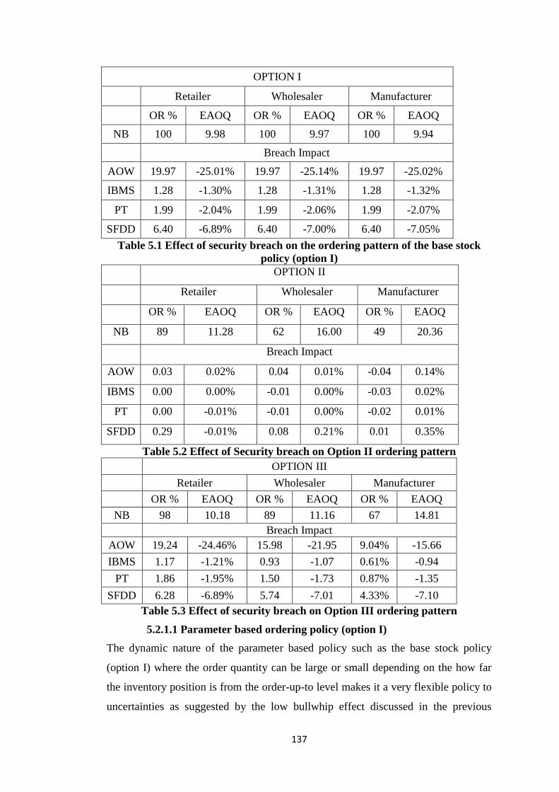
137

OPTION I


OR % EAOQ OR % EAOQ OR % EAOQ

NB 100 9.98 100 9.97 100 9.94

Breach Impact

AOW 19.97 -25.01% 19.97 -25.14% 19.97 -25.02%

IBMS 1.28 -1.30% 1.28 -1.31% 1.28 -1.32%

PT 1.99 -2.04% 1.99 -2.06% 1.99 -2.07%

SFDD 6.40 -6.89% 6.40 -7.00% 6.40 -7.05%

Table 5.1 Effect of security breach on the ordering pattern of the base stock

policy (option I)

OPTION II



NB 89 11.28 62 16.00 49 20.36

Breach Impact

AOW 0.03 0.02% 0.04 0.01% -0.04 0.14%

IBMS 0.00 0.00% -0.01 0.00% -0.03 0.02%

PT 0.00 -0.01% -0.01 0.00% -0.02 0.01%

SFDD 0.29 -0.01% 0.08 0.21% 0.01 0.35%

Table 5.2 Effect of Security breach on Option II ordering pattern

OPTION III



NB 98 10.18 89 11.16 67 14.81

Breach Impact

AOW 19.24 -24.46% 15.98 -21.95 9.04% -15.66

IBMS 1.17 -1.21% 0.93 -1.07 0.61% -0.94

PT 1.86 -1.95% 1.50 -1.73 0.87% -1.35

SFDD 6.28 -6.89% 5.74 -7.01 4.33% -7.10

Table 5.3 Effect of security breach on Option III ordering pattern

5.2.1.1 Parameter based ordering policy (option I)

The dynamic nature of the parameter based policy such as the base stock policy

(option I) where the order quantity can be large or small depending on the how far

the inventory position is from the order-up-to level makes it a very flexible policy to

uncertainties as suggested by the low bullwhip effect discussed in the previous

138

chapter. The ordering pattern is changed to cope with the effect of security breach

whereby order quantity is increased to cope with the sudden demand increase that

the breach creates (recall the assumption in section 5.1.2), which then results in

lower ordering rate. From Table 5.1, one can see that there is a noticeable change in

ordering pattern of all supply chain agents due to the influence of a security breach.

An interesting observation here is that the increase in ordering rate and effective

order quantity is similar for all members despite the fact that the breach occurred at

the retailer. This shows that a breach regardless of its profile has a consistent

reverberating effect on the ordering pattern for all associated supply chain agent

using parameter based ordering (base stock policy). Examining the effect a breach

with high RoC would have on the ordering pattern is done by comparing the effect of

BP1 (low RoC) to BP2 (High RoC) and that of disruption duration is done by

comparing the effect of BP1 (low disruption duration) to BP2 (high disruption

duration). This examination shows that both disruption duration and RoC of a breach

have the same effect on the ordering pattern of the parameter based ordering policy

but the magnitude of effect of RoC is greater.

5.2.1.2 Batch ordering policy (option II)

In contrast to the effect of security breach under the base stock policy (option I), the

ordering pattern of the supply chain using optimal EOQ model (option II) appear to

be unperturbed to a large extent by the breaches as shown in Table 5.2. There seems

to be negligible alteration in the pattern with which supply chain agents place their

orders. In other words the reaction of batch ordering policy to security breach is

minimal or non-existent and as such little or no flexibility is inherent in it. In

addition there is no apparent breach reverberating effect on the ordering pattern of

supply agents as one goes upstream the chain. It is also evident that higher RoC and

disruption duration have no effect on ordering pattern.

5.2.1.3 Combined batch-and-parameter based policy (option III)

The effect of security breach on the ordering pattern of the retailer using option III is

similar to that produced in option I. However the reverberating effect to the

wholesaler and the manufacturer tells a different story and this is shown in Table 5.3.

Common trends emerge for all security breach type. Like option I, the change in

ordering pattern here shows the flexibility inherent in option III. Unlike option I

where the same change occurred throughout the supply chain, the percentage change

139

in ordering pattern (i.e. the ordering rate and the effective order quantity) decreases

as you go upstream. Higher RoC and higher disruption duration produces bigger

changes in ordering pattern with RoC having the greater effect. This seems plausible

as the order size in option III is determined by how far the inventory position is from

the re-order point and a simple economic order quantity is included. Just like option

I, option III ensures to bring the inventory position back to the desired position as

quickly as possible but with an additional EOQ giving it a better capacity to respond

to increased demand. It is to be reminded that the EOQ calculation here is simplistic

(i.e. one batch) and not optimal like option II (2.236 batches). Therefore, option III

combines the flexibility of option I and the advantage of bigger order quantity of

option II. Judging from the level of change produced by option III in response to the

security breaches, one could infer that the ordering policy has some resilience.

However, since the change in ordering pattern is lesser in magnitude to that of option

I, one would expect that the level of security breach resilience would be less than

that of option I. An analysis of the cost impact would serve to confirm this

supposition.

5.2.2 Impact on Cost Performance

The impact of security breach for each ordering option is computed as described in

the opening paragraph of section 5.2 and shown in the subsequent tables for the

various ordering options. The tables include the result of the performance in a non-

breach scenario which is labelled ‘No breach’ and the impact of each breach type is

labelled accordingly.

5.2.2.1 Parameter based ordering policy

Since the base stock policy inherently increases the order quantity and reduces the

ordering frequency to cope with the security breach effect, one would expect a

proportional decrease in daily average ordering cost. This is because a decrease in

ordering frequency decreases the total fixed ordering cost which should result in a

decrease in daily average ordering cost. This is confirmed in Table 5.4 as there was a

2% (AOW), 1% (SFDD), 0.22% (PT), and 0.14% (IBMS) reduction in daily average

ordering cost respectively. This order coincides with the order of ordering rate

reduction AOW>SFDD>PT>IBMS. Those of PT and IBMS approximates to zero as

the change in ordering pattern was very little.

140

Table 5.4 Cost impact of security breach on option I ordering policy (negative

indicates increase while positive indicate a decrease)

The result in Table 5.4 also suggests a breach increases the daily supply chain

holding cost and a proportional decrease in supply chain daily backlog cost, although

this might be different for the respective supply chain agents. The reason for this

observation stems from our assumption in the model that during a breach, the retailer

does not receive any demand information and consequently fulfils only the

outstanding backlogs during this period. This breach period creates a somewhat

‘pseudo-respite period’ for the retailer and wholesaler where all the outstanding

backlog can be fulfilled and any excess inventory received from the upstream agent

during this time is stored, hence the increase in holding cost. After the disruption

period the demand information accumulated during this period suddenly becomes

available and the flexibility of the base stock policy ensures that the supply chain is

able to recover from the increased demand shock by placing orders which reflect the

current state of the operation. The percentage increase in holding cost however is

Holding

£ Backlog £ Ordering £ Total £

Fill

Rate %

No

Breach

Retailer 0.04 140.04 54.83 194.90 0.42

Wholesaler 1.93 55.97 54.80 112.69 0.64

Manufacturer 24.69 5.09 59.62 89.40 0.95

Total 26.66 201.10 169.24 396.99

BREACH IMPACT (Percentage change in cost)


Rate %

SFDD

Retailer -18311 17 1 9 5

Wholesaler -595 18 0 -1 4

Manufacturer -39 -226 1 -23 -9

Total -105 11 1 -1

AOW

Retailer -9705 34 2 23 10

Wholesaler -520 49 2 16 14

Manufacturer -21 65 3 0 3

Total -71 39 2 16

IBMS

Retailer -217 5 0 4 1

Wholesaler -27 7 0 3 2

Manufacturer -2 -3 0 -1 0

Total -4 6 0 3

PT

Retailer -311 7 0 5 2



Total -6 8 0 4

141

highest at the retailer and lowest at the manufacturer for all the security breach

examined, which indicates that the breach reverberating effect on holding cost

reduces as one goes up the chain

Looking at the performance at the operational level of individual agents we see this

impact varies depending on the profile of the breach, that is, the rate of occurrence

(RoC) and the disruption duration. The effect of RoC on all supply agents is quite

similar as their daily average operating cost performances improved with increased

RoC with the manufacturer not faring as well as the other two agents. The only

difference in the observation for the manufacturer compared to those of the retailer

and the wholesaler is that BP1 had a negative impact on the backlog cost of the

manufacturer whereas the impact was positive on the retailer and wholesaler’s

backlog. This observation at the manufacturer is due to the assumption that the

manufacturer has a production lead time of 3 days and transportation lead time of 2

days which means it takes the manufacturer a total of 5 days to get the product to the

wholesaler. Therefore there is no ‘pseudo-respite time’ for the manufacturer to fill

outstanding backlogs. Under BP2 (AOW) however, the manufacturer experienced a

positive effect in its backlog. This is because BP2 (AOW), being a highly frequently

occurring breach, creates a sort of learning curve effect where its repetitive nature

causes the order quantity at each ordering point to be larger than its less repetitive

counterpart (IBMS and PT) thus making the manufacturer carry more inventory.

This increases the fill rate ability of the manufacturer and hence improves its backlog

performance than any other breach type. However the balance between the improved

backlog and increased holding cost does not yield a positive benefit, hence zero

effect of BP2.

Examining the influence of disruption duration, it is obvious that significantly

increasing the disruption duration improves the daily average operating cost

performance of the retailer but this improvement is not as large as the effect of RoC.

However, the effect of disruption duration on the performance of the wholesaler and

manufacturer is a worsening effect. The effect of the longer disruption period in BP3

results in higher holding cost as inventory is held for longer period while the pipeline

inventory satisfies the pre-existing backlog. This causes an improvement in the

backlog cost of the retailer and the wholesaler but the increase in holding cost

outweighs the decrease in backlog cost for the wholesaler. The manufacturer’s

142

backlog is worsened than under BP3. The obvious reason for this is that the

manufacturer does not enjoy the pseudo-respite period that the retailer and the

wholesaler enjoys. Since the disruption period in BP1 (IBMS) is only one day, the

effect on backlog cost is only a 3% increase. However, the disruption period in

SFDD is 5 days creating a bigger effect on backlog cost increase (at 226%).

However the impact on the total supply chain daily operating cost is either positive

or negative depending on the profile of the breach under the base stock policy. BP1

and BP2 both have an oddly positive effect on the total supply chain daily operating

cost with BP2 having the highest positive benefit. Consequently the effect of RoC is

an increase in positive benefit to the supply chain. On the other hand, BP3 had a

negative effect, therefore comparing BP1 to BP3 suggest that the effect of disruption

duration is a worsening of supply chain daily average operating cost performance as

shown in Table 5.4.

The general observation under the parameter based ordering policy such as the base

stock policy is that the reverberating effect of BP1, BP2 and BP3 increases as one

goes upstream the chain, although BP1 and BP2 have an oddly positive effect on

retailer and wholesaler’s performance. It is also clear that increasing RoC of a breach

produces a resultant positive effect on supply chain daily total operating cost while

disruption duration produces a resultant negative effect.

5.2.2.2 Batch ordering policy (option II)

Although being an optimal EOQ model under normal circumstances, the order

quantity produced under option II is somewhat the same and does not change

significantly to cope with the effect of the breach. This means that the effect of the

pseudo-respite period would be negated by the inability of the policy to increase

order quantity to satisfy the relatively large demand coming in after the disruption

duration. Therefore, in contrast to option I where the pseudo-respite period effect led

to a reduction in backlog cost, the inflexibility or lack of resilience of option II

would result in a backlog cost rise. The impact of each security breach on supply

chain using option II ordering policy is shown in Table 5.5. The performance under a

non-breach scenario and the percentage rise or fall in cost performance and fill rate

performance under each security breach is shown.

143

Table 5.5 Cost impact of security breach on Option II ordering policy (negative


Suffice to say that the ordering cost is expected to stay the same if no changes occur

to the rate and quantity of the orders. Considering that there was no change in

ordering pattern, the daily average ordering cost of all supply chain agents was not

impacted by any of the security breaches. The impact of all the security breaches,

however, was a rise in total supply chain holding cost and backlog cost. The level of

impact again differs for each supply chain agent depending on the profile of the

breach. Also, the reverberating effect tends to decrease as one goes further upstream.

Again, to examine the effect of RoC on individual performance, it is evident that that

increasing the RoC of the breach worsens the performance of the retailer but has no

apparent effect on the performance of the wholesaler and manufacturer. On the other

hand, increasing the disruption duration worsens the performance of all supply

agents with the retailer worse off and the manufacturer least affected. However,

Holding £ Backlog £ Ordering

£ Total £

Fill

Rate %

No

Breach

Retailer 2.41 63.35 54.25 120.00 0.61

Wholesaler 16.98 16.90 52.93 86.81 0.86

Manufacturer 39.21 9.07 54.68 102.96 0.92

Total 58.60 89.32 161.85 309.77

BREACH IMPACT(Percentage change in cost)


Rate %

SFDD

Retailer -327 -225 0 -125 -29

Wholesaler -27 -100 0 -25 -11

Manufacturer -4 -35 0 -4 -3

Total -24 -182 0 -57

AOW

Retailer -29 -41 0 -22 -8

Wholesaler -3 -9 0 -2 -1

Manufacturer 0 3 0 0 0

Total -2 -30 0 -9

IBMS

Retailer -15 -5 0 -3 -1


Manufacturer 0 -2 0 0 0

Total -1 -5 0 -2

PT

Retailer -18 -10 0 -6 -2


Manufacturer 0 -2 0 0 0

Total -1 -8 0 -3

144

examining the effect of the breach profile on supply chain performance, it is clear

that disruption duration has a very large effect on supply chain performance than

RoC with both producing a negative effect.

In conclusion, the breach reverberating effect diminishes under BP1, BP2 and BP3

as one goes upstream the chain. Increasing the RoC only negatively affects the

performance of the retailer and this effect produces a resultant negative effect on the

entire supply chain performance while increasing the disruption duration of the

breach increases the negative impact a breach has on the supply chain and all its

members.

5.2.2.3 Combined batch-and-parameter based policy (option III)

The impact of each security breach on supply chain using option III ordering policy

is shown in Table 5.6. Like option I, BP2 and BP3 caused a very significant

reduction in the ordering rate of option III which led to a significant reduction in the

daily average ordering cost of supply agents. On the other hand, the reduction of the

ordering rate due to BP1 is not large enough to offset a change in daily average

ordering cost of the supply chain under the combined batch-and-parameter based

ordering policy (III). Considering the impact of these breaches on other cost

performance measures (as shown in Table 5.6), the holding cost of all supply agents

was increased, as expected, but the effect on backlog differed based on the breach

profile.

In general the combined batch-and-parameter based ordering policy behaves like the

parameter based policy under information security breach but retains the optimality

that the additional EOQ component provides. Therefore the impact of a security

breach on its performance is generally in between the performance of parameter

based and batch ordering policies under the same breach.

The main observation here (Table 5.6) is that increasing the RoC negatively affects

the performance of all the supply agents, although the effect is not very large. An

increase in the disruption duration on the other hand negatively affects supply

agents’ performances and this effect is greater than the effect of RoC. Interestingly,

the reverberating effect of a breach of the type BP1 increases only slightly, as one

goes up the chain while BP2 and BP3 increases and then decreases after the

wholesaler tier.

145

Table 5.6 Cost impact of security breach on option III ordering policy (negative



This study has shown that priorities as to which element of the breach profile

(disruption duration or RoC) should be addressed depends on the ordering policy of

choice. This would also inform which aspect of risk management measures to

prioritise. For a parameter based ordering policy, increased RoC only increases the

positive effect of a breach on the performance of the parameter based ordering policy

while disruption duration increases the negative effect. Therefore supply chain

priority for such parameter based ordering policy would be to focus on reducing the

disruption duration of a breach, hence breach correction or mitigation would be a

priority. The priority for a supply chain with batch ordering policy and that for a

combined batch-and-parameter based ordering is also breach mitigation as disruption

duration had a greater effect on breach cost impact than RoC.

Holding

£ Backlog £

Ordering

£ Total £

Fill

Rate %

No

Breach

Retailer 1.94 50.01 54.73 106.68 0.67

Wholesaler 12.90 12.56 54.26 79.72 0.89

Manufacturer 56.60 0.60 56.30 113.50 0.99

Total 71.44 63.17 165.28 299.90

BREACH IMPACT(Fractional change in cost)


Rate

SFDD

Retailer -621 -12 1 -17 -3

Wholesaler -129 -78 0 -33 -7

Manufacturer -13 -1475 1 -14 -8

Total -51 -39 1 -20

AOW

Retailer -553 21 2 1 5

Wholesaler -116 33 1 -13 3

Manufacturer -10 68 2 -4 0

Total -44 24 2 -5

IBMS

Retailer -37 7 0 3 2


Manufacturer -1 -15 0 0 0

Total -3 7 0 1

PT

Retailer -50 8 0 3 2



Total -5 9 0 1

146

The breach cost impact reverberating effect differs for the three ordering options

considered. The effect consistently increases for all three breach profiles considered

under the parameter based policy while the effect consistently decreases under the

batch ordering policy. Under the combined policy however, the reverberating effect

increases slightly when faced with breach of type BP1 and the effect increases and

then decreases at the manufacturer. Therefore supply chains using the parameter

based ordering would be more wary of information security breach occurring

downstream in the supply chain than those using batch ordering policy. In a supply

chain using the combined policy type, the wholesalers should be particularly wary of

information security breach occurring downstream. In all, members of the supply

chain existing in the upstream part of the supply chain would be affected by

information security breach occurring at the downstream side of the chain due to the

reverberating effect of the breach. This study therefore calls for better cooperation

among supply partners and supports the claim that information security breach

incidence and data should be shared between supply chain partners. This would help

the non-breached, but affected, partners better prepare for eliminating or reducing

the reverberating effect of such breach.

Finally, recall from the previous chapter that under normal circumstances (i.e. no

security breach), the batch ordering policy performs better than the parameter based

ordering policy. However in this chapter, the result has shown that the parameter

based policy outperforms the batch ordering policy when breach RoC is high (BP2)

or disruption duration is high (BP3). However when the breach is of the type BP1,

the batch ordering policy still outperforms the parameter based ordering policy. The

combined batch-and-parameter based policy performs best in both breach and non-

breach situations. So far the performance of each ordering policy under information

security breach has been assessed in a serial non-information sharing scenario (i.e.

the base model). The next section evaluates the effect supply chain structural

reconfiguration strategy has on the impact of information security breach. The

question here is; can structural reconfiguration be used as a cost mitigation strategy

even under disruption situations caused by information security breach?

147

5.3 STRUCTURE EFFECT ON BREACH IMPACT

To estimate the mitigating effect of supply chain structure on the impact of security

breach, the difference between the impact of security breach on the base model and

that of the reconfigured scenario relative to the base model is computed. First the

impact of security breach on the base model is calculated and expressed as a

percentage (as explained in section 5.2). Then the impact of security breach on the

reconfigured scenario relative to the base model is computed (also expressed in

percentage). The difference between these two percentages is an estimation of how

much reduction in breach impact can be derived when structural reconfiguration is

adopted. This method of computation is used because it ensures that all the breach

impacts computed have a common relative point (the base model with no breach)

which makes the impact mitigation percentage comparison between structures more

direct and accurate. This percentage difference is termed ‘structure effect on breach

impact’ (SEOBI) and is tested for significance at p<0.05 to show whether the effect

of SEOBI is statistically significant at p<0.05 or not. If the SEOBI is not significant

at p<0.05, then SEOBI is said to be non-existent. Otherwise the effect is said to be

existent. The direction of the effect on operating cost can be of a positive type

(mitigating), a negative type (exacerbating) or neither (stabilising). A negative value

reveals an exacerbating effect while a positive value indicates a mitigating effect. A

non-significant value shows that the structure effect is of a stabilising nature

regardless of it being either positive or negative. The SEOBI on each supply agent

for each of its performance measures (daily average holding, backlog, ordering

costs) and that on the entire supply chain is computed for each ordering policy.

However all the tables shown in this section only include the effect on total daily

average operating cost of each agent (R- retailer, W- wholesaler, M- manufacturer)

and not the individual daily average costs. The values with superscript ‘nd’ indicate

that the percentage difference is not statistically significant at p<0.05.

5.3.1 WH Structure Effect on Breach Impact

The result shown in the Table 5.7 is the percentage change between the performance

of a serial chain under security breach and that of a wholesaler structure type under

security breach.

148

SFDD

R. Cost % W. Cost % M. Cost % SC Total %

option I -4 6 19 4

option II 60 21 10 32

option III 10 30 13 16

AOW


option I -10 -2nd 5 -5

option II 8 9 7 8

option III -4 13 4 4

PT


option I -5 -2nd 6 -2nd

option II 0nd 9 7 5

option III -1nd 11 4 4

IBMS



option II -1nd 9 7 4

option III 0nd 11 4 4

nd- means no significant difference at p<0.05

Table 5.7 Percentage change in impact due to wholesaling simplification

5.3.1.1 Influence of WH under Option I Scenario

As revealed in Table 5.7, the WH structure has a mitigating effect under option I

when a very disruptive security breach (BP3) is encountered with a 4% reduction in

SFDD breach impact. However, WH effect makes the impact of a less disruptive but

highly recurring breach (BP2) on supply chain performance worse than it would be

in a serial supply chain i.e. exacerbating effect. The exacerbating effect under the

less disruptive and less recurring breaches PT and IBMS (BP1) is not significant,

hence considered to be a stabilising effect. Therefore WH structure has a stabilising

effect on less disruptive, less recurring breaches but when the RoC is at higher levels

an exacerbating effect is seen.

At the operational level, the WH structure has an exacerbating impact on the

retailer’s total operating cost performance under highly disruptive and less disruptive

breaches. However, the WH-exacerbating effect is not increased with increasing

disruption duration but increasing the RoC does. For the wholesaler, WH structure

has a mitigating effect under a highly disruptive breach and a stabilising effect under

a less disruptive breach. The stabilising effect is not affected by increasing the RoC

of the breach. The impact of both highly disruptive and less disruptive (but highly

149

occurring) breaches on the manufacturer’s total operating cost performance is

mitigated under WH structure. This mitigation effect is seen to increase as the

disruption period increased (between IBMs and SFDD). RoC however does not seem

to have any impact on the mitigating effect of WH structure on manufacturer’s total

operating cost performance.

5.3.1.2 Influence of WH under Option II Scenario

At the supply chain level, the WH structure appears to hold significant benefit over

the serial structure both in no-security breach and security breach scenarios. Under

all the security breach scenarios considered, a WH-mitigating effect is observed as

shown in Table 5.7. The mitigating effect is highest under a more disruptive breach

(SFDD) than a less disruptive one (IBMS). Comparing the mitigating effect under

AOW (8%), PT (5%) and IBMS (4%) reveal that increasing the RoC increases the

mitigation WH structure stand to offer.

At the operational level, the retailer enjoys a mitigation of the impact of a very

disruptive breach on its daily operating cost performance under WH structure. For

less disruptive breaches such as IBMS and PT, an exacerbating effect is felt at the

retailer’s end, however not significant (stabilising effect). The exacerbating effect,

although insignificant, is seen to reduce as RoC increases. However, this changes to

a mitigating effect when RoC is significantly increased as in the case of AOW

breach (at approximately 8% mitigation). The wholesaler and the manufacturer on

the other hand enjoys a mitigation effect regardless of the breach type. They both

enjoy higher mitigation levels under a more disruptive breach (SFDD) than less

disruptive ones. The mitigation level is however not significantly affected by RoC

increase.

5.3.1.3 Influence of WH under Option III Scenario

The WH structure is also favourable towards ordering policy of the type ‘option III’

in the event of the security breaches mentioned. As shown in Table 5.7, regardless of

the nature of the breach, the WH structure has a mitigating effect on the magnitude

of the impact of highly disruptive and less disruptive breaches. Higher levels of

mitigation occur when the breach is highly disruptive than when the breach is less

disruptive. A higher level of RoC does not seem to congruently affect the mitigation

150

level, although this appear to reduce with increasing RoC. However the rate of

change of the mitigation level does not correspond with the rate of change of RoC.

At the operational level of the supply chain, mitigating effect is only seen to occur

under a highly disruptive breach (10%) at the retailer’s end while the effect to the

retailer’s daily operating cost is of an exacerbating nature under a less disruptive

breach. Although the exacerbating level under PT and IBMS is insignificant at

p<0.05, the level is however significant under a breach with much higher RoC

(AOW). Therefore for a less disruptive breach, the exacerbating effect is

insignificant at lower RoC but become significant with significantly higher RoC. On

the hand, the wholesaler and the manufacturer both enjoy a WH-mitigation of

security breach impact on their respective daily operating cost performance. While

they both enjoy increased mitigation under a highly disruptive breach (comparing

SFDD to IBMS), the mitigation level enjoyed by both agents is unaffected by

increased RoC. Therefore, for the wholesaler and manufacturer, RoC has no effect

on the magnitude of mitigation derivable from a WH structure.

5.3.1.4 Summary and Implication of Finding

This section has established that reconfiguring the supply chain from the serial

structure to the WH configuration can provide benefit both in a security breach

scenario and in a non-security breach scenario. This benefit of course depends on the

ordering policy of choice and the profile of the breach.

Under option I scenario, WH effect is inconsequential when a breach of the type BP1

occurs but becomes disadvantageous when the breach in question has a high

recurrence rate. However, it provides a mitigation benefit when the disruption

duration of the breach is high. Therefore the implication of this to the IT manager is

that when WH structure is adopted, then more focus is needed in breach prevention

and deterrence rather than breach mitigation measures.

For option II and III, WH effect provides mitigation benefits to the supply chain.

Even in the event of that the disruption duration or recurrence rate of the breach

increases significantly, WH structure provides increased mitigation benefit.

Therefore the cost benefit from reconfiguration can be used to upgrade or augment

existing risk prevention and mitigation tools that were previously unaffordable. This

151

in turn would help prevent future attack from occurring or mitigate it better when it

occurs and further cost savings can be derived.

5.3.2 MF Structure Effect on Breach Impact

The values presented in in Tables 5.8 represent the percentage increase (if negative)

or decrease (if positive) in impact cost due to the Manufacturing Structure (MF)

effect.

SFDD


option I -4 2nd 25 4

option II 60 13 15 32


AOW


option I -12 -8 11 -6

option II 8 1nd 13 8


PT


option I -3nd -2nd 11 1nd

option II 0nd 0nd 13 4

option III -3 0nd 6 2

IBMS


option I -2nd -1nd 11 1nd

option II -1nd 0nd 13 4

option III -2nd 0nd 6 2


Table 5.8 Percentage change in impact due to manufacturing simplification

5.3.2.1 Influence of MF under Option I Scenario

Considering the profile of a security breach in terms of the disruption duration and

the frequency with which the breach occurs (also known as RoC), the mitigating role

of MF structure is more favourable towards the disruption duration than RoC. In fact

as Table 5.8 suggest, MF effect responds negatively to increasing RoC. From the

result it is apparent that under high RoC, the stabilising effect of MF diminishes and

an exacerbating effect is seen. Based on disruption duration, MF structure tend to

have a mitigating influence on the impact a highly disruptive breach has on supply

chain daily operating cost. The stabilising effect of MF structure under BP1

improves and becomes a mitigating type under BP3, confirming that MF effect is

more favourable towards a breach with higher disruption duration.

152

Looking at the performance of individual supply chain agents under security breach,

the retailer is not favoured under the MF structure effect. The performance of the

retailer is worsened under the MF structure revealing that MF has an exacerbating

effect on how security breach impacts the retailer. In fact this performance is made

worse under higher levels of disruption duration and RoC. Interestingly for the

wholesaler, a statistical test shows MF structure has a stabilising effect on the impact

of a highly disruptive breach. In other words increasing the disruption duration has

no impact on the stabilising effect of the MF structure on wholesaler daily operating

cost performance. RoC however has an impact on the stabilising effect of MF. The

MF effect on the performance of the wholesaler under a breach of type BP1 is of a

stabilising nature, however this stabilising effect diminishes as RoC increases

significantly resulting in an exacerbating effect. The manufacturer on the other hands

benefits from the MF effect especially under a more highly disruptive breach. The

MF structure has a mitigating effect on the impact of security breach on

manufacturer’s daily operating cost. The level of mitigation is unaffected by varying

levels of RoC but is increased under higher disruption duration.

5.3.2.2 Influence of MF under Option II Scenario

At the strategic level (that is the supply chain level), a mitigation of the impact of

security breach on supply chain cost performance is observed regardless of the

security breach profile as shown in Table 5.8. The more disruptive the breach the

better the mitigation effect derivable and the higher the RoC the higher the

mitigation level.

At the operational level (that is the individual supply chain agent level), the retailer

either experiences a stabilising effect or a mitigation effect depending on the profile

of the breach. For a less disruptive breach such as PT and IBMS, the retailer

experiences a stabilising effect. However this stabilising effect transmogrify into a

mitigating type when the RoC is significantly increased as in AOW (8%). For the

more disruptive breach type (SFDD) a mitigation effect is observed at the retailer’s

end. The MF effect changes from a stabilising nature to a mitigation type when the

disruption duration of the breach increases significantly as revealed by the

comparison between the influences on IBMS (stabilisation at 1%) and SFDD

(mitigation at 60%). The influence on the wholesaler breach performance again

depends on the profile of the breach. This influence is positive for a more disruptive

153

breach and neutral for a less disruptive type. Therefore, regardless of the RoC level

of the less disruptive breaches, MF consistently had a stabilising effect on the impact

of this breach type on wholesaler daily operating cost performance. However, this

influence goes from a stabilising 0% under IBMS (a less disruptive breach) to a

mitigating 13% under SFDD (a more disruptive breach). This again shows that the

wholesaler enjoys greater mitigation influence when the disruption duration is

increased and maintains a stabilising effect even if the RoC is increased

significantly.

The manufacturer enjoys a mitigation of the impact of security breach under the MF

structure. The mitigating influence of MF on the impact of security breach on the

manufacturer’s daily operating cost is not significantly perturbed by increasing RoC

and increasing disruption duration. As shown by the result the mitigation level

remains at the same level for AOW, PT and IBMS, while there is only a slight

increase in mitigation level between IBMS and SFDD and this slight increase is not

commensurate with the increase in disruption duration.

5.3.2.3 Influence of MF under Option III Scenario

The supply chain enjoys an improved cost performance in the event of a security

breach when the MF structure is preferred over the serial structure type as shown in

Table 5.8. Regardless of the breach profile, a mitigation effect is observed on supply

chain performance; meaning the worse the breach gets, the better is the derived

benefit. Worsening the breach by increasing the RoC or the disruption duration

further increases the benefit derived from MF structure. Although a slight increase in

RoC (comparing IBMS and PT) does not change the level of mitigation, however, a

significant increase in RoC level produces a reasonable increase in mitigation effect.

There is no tangible effect of MF structure on the impact of less disruptive breaches

on the retailer’s daily operating cost performance, however for more disruptive

breaches the effect is tangible. Increasing disruption duration means the MF structure

is able to provided added benefit to the retailer with structure influence going from

stable under BP1 to higher mitigation under BP2. Increasing RoC has no consistent

effect on the influence MF has on retailer’s cost impact. There is tangibility in the

effect disruption duration and RoC has on the way MF influences the wholesaler’s

cost impact. Increasing breach RoC slightly does not change the level of influence

154

MF has on wholesaler’s performance, however, a significantly elevated RoC

produces a marked improvement in MF mitigation effect. Again, the wholesaler in

the MF structure reacts much better than one in the serial counterpart to increased

disruption duration of information security breach. For the manufacturer however, a

step change in RoC only slightly improves the mitigation effect of MF structure.

Increased disruption duration from one day to five days changes the level of

mitigation on manufacturer’s cost impact from 6% to 16%.


Like the WH structure, the MF structure also influences the way the supply chain

reacts to demand and also to information security breach. The result has further

strengthened the argument that ‘susceptibility’ of an ordering policy to structural

change determine how much breach impact mitigation the supply chain is able to

enjoy when such structural changes are made. Under the manufacturing structure,

option I was the least susceptible to structural and option II was the most susceptible

while option III was median susceptible in a non-breach scenario. The result from

this section has shown that the mitigation level of MF configuration towards option

II performance is highest followed by option III with option I deriving the least

benefit, confirming the argument.

It has also been established that reconfiguration from a serial structure into a

manufacturing structure holds benefit to the supply chain in a non-breach and breach

scenarios. In the breached scenario, the level of benefit depends on the ordering

policy and the breach profile.

Under option I, changing to a MF structure ensure that the supply chain would enjoy

a reduction in impact cost when a more disruptive breach occurs although the MF

structure has no significant effect when the breach in question is of a less disruptive

type. However, under option I, the MF structure is not able to provided benefit to the

supply chain and in fact exacerbates the impact cost when the breach recurrence rate

is significantly high. This therefore implies that upon changing to this structure type,

the prevention and deterrence measure would require more focus than they would in

a serial chain.

For option II and III, MF structure brings about a mitigation of breach cost impact

for the supply chain. Therefore, cost benefit of MF structure under security breach

155

exists regardless of the breach profile whether disruption duration or RoC is high or

low. The implication of this therefore is that the impact cost benefit derived can be

redirected towards improving IT security which will yield added benefits on the long

run.

5.3.3 Network Structure Effect on Breach Impact

This section evaluates how the magnitude of security breach impact is changed by

network reconfiguration under the three ordering options. The network effect (NT-

effect) on breach impact is shown in Table 5.9.

SFDD


option I -4 4 19 3

option II 58 16 15 32


AOW


option I -10 -4 5 -5

option II 7 6 12 9

option III -4 11 5 3

PT


option I -5 -4 6 -2



IBMS






Table 5.9 Percentage change in impact due to network configuration

5.3.3.1 Influence of Network Structure under Option I Scenario

Under the network structure, the impact of the security breach on supply chain cost

performance is only alleviated when the breach has a higher level of disruption

duration as shown in Table 5.9. This is seen in SFDD where the influence of NT-

structure is a mitigation type at 3% compared to IBMS which is of a stabilising

nature at -2%. However, the influence becomes an exacerbating type when the RoC

of the breach increases as evidenced by the result of AOW, PT and IBMS.

156

A similar trend is observed for the wholesaler where N-effect causes a mitigation of

the impact a highly disruptive breach (SFDD, 4%) has on wholesaler’s daily

operating cost performance. The effect on the less disruptive breach type (IBMS, -

4%) is not significant but is significant under high RoC (AOW, -4%). Therefore,

under this structure, the wholesaler should be more wary of increase in RoC rather

than disruption duration. The retailer does not benefit from the N-effect and in fact

the N-effect makes impact worse when disruption duration and RoC are increased as

the result suggest. The manufacturer on the other hand enjoys a mitigation benefit

from the N-structure configuration. The benefit to the manufacturer’s daily operating

cost performance increases under increased disruption duration but this benefit

appears unperturbed by increasing RoC.

5.3.3.2 Influence of Network Structure under Option II Scenario

At the supply chain level, the effect of reconfiguration from a serial structure to a

network structure brings benefit to the way the supply chain is impacted by security

breach. The impact of information security breach on a supply chain with network

type configuration would fare better than one with serial configuration. This

observation is evidenced from the result in Table 5.9 where the percentage change in

impact from serial to network structure is positive for all the security breach types.

That is, NT-effect on supply chain cost performance is of a mitigation nature rather

than stabilisation or exacerbation nature. It is also clear that the level of mitigation is

in turn influenced by the profile of the breach in terms of disruption duration and rate

of occurrence (RoC). The mitigating effect of NT-structure in seen to increase

significantly under a breach with higher disruption duration when the result for

IBMS (5%) is compared to that of SFDD (32%). In the same light the mitigating

effect also increase under increased RoC when IBMS (5%), PT (5%) and AOW (9%)

are compared.

At the operational level in the supply chain, the benefit to the retailer only comes

when the breach is more disruptive and highly prevalent. N-effect has a stabilising

influence on the way the retailer’s daily operating cost is impacted by less disruptive

and less frequently occurring breaches in a serial supply chain. However when the

breach is more disruptive or recurring, the benefit to the retailer is increased and a

good mitigation level is seen especially when the breach is more disruptive. The

story is somewhat different for the wholesaler. Although the wholesaler enjoys a

157

mitigation of the security breach impact cost, this mitigation level only significantly

increased under increased disruption duration but not RoC. Therefore, there is no

increased N-effect benefit to the wholesaler under increased breach RoC, or at least

the step increase in RoC is not commensurate with the increase in benefit. A similar

observation to that of the wholesaler is found at the manufacturer’s end. Although

there is an observed mitigation effect on manufacturer’s daily operating cost

performance, the level of mitigation is not commensurate to the level of increase in

disruption and RoC levels. Therefore there is no apparent increase in benefit to the

manufacturer if the profile elements of the breach (that is disruption duration and

RoC) is raised.

5.3.3.3 Influence of Network Structure under Option III Scenario

The influence of the network structure on option III is also shown in Table 5.9. A

mitigating effect is observed at the supply chain level for all breach types. This

mitigation level is increased between IBMS (3%) and SFDD (15%). Confirming that

an increased disruption duration does not worsen the role N-effect plays in

mitigating breach cost impact, but in fact reveals that N-effect has higher

counteracting effect. The result also shows that the mitigation level is not

significantly changed between IBMS (3%), PT (3%) and AOW (3%). Confirming

that the counteracting effect of N structure is not affected by increased RoC.

For the retailer, the N-effect stabilises the impact of a less disruptive breach type on

its daily operating cost performance. However this stabilisation diminishes when the

RoC of the breach increases and an exacerbating effect is observed. For a more

disruptive breach, the observed stabilising effect of the network structure is

strengthened and the breach impact is further absorbed by the structure creating a

mitigating effect. The wholesaler and the manufacturer both enjoy a mitigation of the

impact of security breach on their daily operating cost performance. Both agents also

enjoy an increase in the mitigation level in the event of increased disruption duration.

However the benefit to the manufacturer appear to be unaffected by increased RoC

while that to the wholesaler is. The wholesaler enjoys better performance under a

breach with significantly high RoC as shown by the AOW result.

158


This section further validate the argument that supply structure play a mitigation role

on the way security breach impact the supply chain.

Under ordering option I, the network structure has an exacerbating effect on supply

chain performance when faced with a less disruptive breach and this negative effect

increases when RoC increases. This effect however diminishes and becomes a

mitigating effect when the breach becomes more disruptive. The implication of this

is that upon transformation into the network structure, more attention need to be paid

to improving the breach prevention and deterrence strategy than breach correction

strategy.

With option II, the N-effect result in a mitigation of security breach impact on supply

chain performance and the level of mitigation increases when faced with more highly

disruptive or recurring breach. Consequently, the IT manager need not worry about

raising IT security effort because of structural change. In fact reconfiguring the chain

into a network type structure generates benefits that can be redirected into fortifying

IT security.

For option III, the network structure improves the response of the supply chain to

breach impact by mitigating the cost impact. The level of mitigation increases when

the disruption duration of the breach significantly increases but the remains at the

same level when RoC significantly increase instead. This implies that the mitigated

cost can be re-invested into improving the security level.


The decision framework of whether to accept the improvement strategy as breach

cost impact mitigation strategy for each supply agent is shown in Figure 5.2.

159

Figure 5.2 Single strategy acceptance decision framework in a breach scenario

First the cumulative effect of structural reconfiguration on breach impact for each

scenario is computed and if this computation is positive then the strategy has a

mitigating effect and is therefore acceptable, otherwise it is not acceptable. The

reverberating effect is understood by computing the cumulative effect of the

improvement strategy for each supply agent and then examining if this increases or

decreases along the supply chain. If the reverberating effect decreases but is still

significant upstream, then perhaps the retailer should immediately notify the

upstream partners of any breach so they can quickly respond to the effect such

breach might have. This is known as information security breach (ISB) sharing. If,

on the other hand, the reverberating effect of the breach increases or if the impact

experienced at the retailer is less than that experienced upstream, then the affected

party should be provided with some form of breach impact incentive in addition to

the incentive that ought to be provided under normal circumstances considering the

type of improvement strategy. This should also be done in addition to timely sharing

of security breach information. However if the impact upstream is not significant

then no incentivisation or ISB sharing from the retailer is required. Therefore

reverberating effect has implication to ISB and incentivisation decision within the

Does the improvement strategy have a mitigating

effect on breach cost impact?

Reverberating effect on

supply chain agent?

Is the agent directly involved

in the strategy change?

Yes

Increasing effect

No Yes

No

Decreasing effect

No effect

Accept

strategy

with only

ISB sharing

Accept

strategy with

incentive and

ISB sharing

No ISB

sharing or

incentivisat

ion

Accept

strategy

Reject

strategy

160

supply chain. On the other hand understanding the effect of high RoC and disruption

duration is important to knowing where Information security management (ISM)

priorities lie. If a change in disruption duration from low to high has a greater

negative effect than that of RoC for any supply chain scenario, then IT priority

would be on corrective measures (C), otherwise the priority would be prevention &

deterrence (P&D).

The summary of the result is shown in Table 5.16. The decision to accept an

improvement strategy is based on whether the aggregate benefit derived from the

non-breach scenario (n-BS) and the breach scenario (BS) is positive or not and the

implication to ISB sharing; additional breach impact incentivisation; and information

security management (ISM) priority is also indicated. The general observations are

listed below:

Structural reconfiguration by itself does not mitigate the impact information

security breach has on supply chain performance for a parameter based

policy (option I) but instead makes it worse. The only exception is the MF

structure where benefit is derivable and the retailer needs to share ISB

information with the wholesaler.

Reconfiguration will prove beneficial to batch ordering systems (option II)

and batch-and parameter based policy (option III) in a security breach

scenario but ISM focus should be on prevention and deterrence rather than

corrective measures. In addition, there is no need for ISB sharing and

incentivisation after a security breach.

Similar to the non-breach scenario, the serial structure is again preferred

under parameter based ordering policy while the networking strategy and the

wholesaling simplification strategy are the best cost performers under batch

and batch-and-parameter based policies respectively.

ISM priority would be to focus more on prevention and deterrence when any

of the structural reconfiguration strategies is adopted.

161



n-BS

Benefit 0% 3% 0% 3% 3% 4% 5% 2% 4%

BS Benefit -3% 1% -6% 50% 48% 51% 29% 22% 25%

Total

Benefit -3% 4% -6% 53% 51% 55% 34% 24% 29%

Acceptable? No Yes No Yes Yes Yes Yes Yes Yes

ISB sharing

with? - W W - - - - - -

Incentive

to? - - - - - - - - -

IT priority P&D P&D P&D P&D P&D P&D P&D P&D P&D

Table 5.10 Summary and implication of supply reconfiguration to information

security breach impact

5.4 INFORMATION SHARING LEVEL EFFECT ON BREACH IMPACT

Information sharing level has been established in the previous chapter to provide

benefit for certain supply chain members which can be shared with non-benefiting

counterparts. The magnitude or direction of such benefit may be compromised by the

incidence of information security breach. For all the benefits and performance

improvement brought about by information sharing in a non-breach scenario, this

study aims to determine whether this benefits are still applicable in a breach scenario

and how the landscape of benefit changes. This study propose that based on the

magnitude and direction of breach impact, the decision to engage in any level of

information integration should not be taken until after breach impact considerations.

To estimate the benefit of information sharing, if any, in the face of security breach,

the performance under an information sharing mode with breach is compared to that

under a non-information sharing mode (NI-base model) with breach. The analyses

here is similar to that in section 5.3, the only difference is that information sharing

level (ISL) influence on breach impact is being considered instead of structure effect.

Therefore the tables used in this section are derived in a similar fashion to those in

section 5.3. Again, the influence of information sharing level on information security

breach impact is examined to see if it is of a mitigating, exacerbating or stabilising

162

nature. A mitigating effect is such that the breach cost impact in a supply chain that

has engaged in information sharing is significantly lower (at p<0.05) than that of the

non-information sharing counterpart. An exacerbating effect is seen when the breach

impact in the information sharing mode is significantly higher (at p<0.05) than that

of the base model. A stabilising effect on the other hand occurs when there is no

significant difference (at p<0.05) between the breach impact in both information

sharing and non-information sharing scenarios. The values with superscript ‘nd’

indicate that the percentage difference is not statistically significant at p<0.05.

The pattern of analysis has been established throughout section 5.3. Therefore in this

section the summary of the finding is given without going into details of how the

analysis is done as this has been established already. Consequently, for each ISL, the

MES effect is identified followed by the response of ISL to changing breach profile.

In conclusion, the effect of increasing disruption duration and RoC is identified and

the implication to information security management and supply chain inventory

management is drawn.

5.4.1 Influence of RW on Breach Impact

The influence of having a RW level of information sharing when four main types of

breach occurs is revealed in Table 5.11. Its effect on each supply agent and the total

effect on supply chain operating cost for each ordering policy type is shown. Under

the highly disruptive breach, RW mitigates the breach impact on an option I supply

chain but the effect on the wholesaler and retailer is of the stabilising type while the

manufacturer enjoys mitigation. In this case, RW mitigates the impact only at the

upstream of the supply chain. Under a less disruptive breach however, RW mitigates

the impact on supply chain operating cost with the retailer and wholesaler this time

enjoying a mitigation while the manufacturer is unperturbed at p<0.05. Here RW has

no significant influence on the impact of a less disruptive breach on the performance

of the upstream part of the chain. The result in Table 5.11 suggest that RW is not

very favourable to the supply chain when the breach is very disruptive (SFDD) but

better mitigation is derived when the supply chain experiences a less disruptive kind.

Examining the disruption duration effect and the RoC effect, the higher the

disruption duration of a breach the lesser the derived benefit from RW configuration.

The higher the RoC of a less disruptive breach, the lesser the derived benefit,

although the margin is not very high. However the manufacturer appear to enjoy

163

more mitigation form RW when the RoC increases significantly. The implication of

this finding is that although RW mitigates the impact of security breach on option I

supply chain, more effort should be put in the breach mitigation than in the

prevention measures.

SFDD


option I 0nd 0nd 8 2

option II 22 -8 -14 2nd

option III -8 -1nd 10 1nd

AOW


option I 6 2 12 6

option II 12 -6 -2nd 2nd

option III 4 0nd 13 6

PT


option I 10 15 -1nd 9

option II 7 4 -3nd 3

option III -3 -2 13 3

IBMS


option I 10 15 -2nd 9




Table 5.11 Percentage change in impact due to RW ISL for all three ordering

policy scenarios

Under option II scenario, the impact of the more disruptive and less recurring breach

(SFDD) and the more recurring and less disruptive breach (AOW) on total supply

chain performance were stabilised at p<0.05. Interestingly, the impact of the less

disruptive and less recurring breaches (PT and IBMS) were mitigated with RW

information sharing level. At the operational level, RW mitigates the impact of a

highly disruptive breach on the retailer’s average daily operating cost performance

but the impact on the wholesaler and the manufacturer was in fact exacerbated.

However, for the less disruptive breaches the retailer and wholesaler enjoys a

mitigation while the manufacturer experiences a stabilising effect. When the RoC

increases (as in the case of AOW), the obvious effect is on the wholesaler

performance as it changes from mitigation to exacerbation. Overall, for breaches

with high disruption duration and high RoC, RW does not provide any breach impact

mitigation but it is only beneficial when the breach is less disruptive and has a low

164

recurring rate. Consequently the breach management effort need not be increased

due to RW reconfiguration. However, any further efforts, if any, should be geared

towards improving both prevention and mitigation measures.

For option III, RW stabilises the impact of a very disruptive breach on supply chain

performance but mitigates the impact when the breach is less disruptive. When the

less disruptive breach becomes more recurring the mitigation benefit of RW

increases. At the operational level, the impact of a highly disruptive breach on the

retailer, wholesaler and manufacturer is exacerbated, stabilised and mitigated

respectively by RW. Under the less disruptive breach scenarios (PT and IBMS), the

effect of RW is of the exacerbating type on the retailer and the wholesaler while the

manufacturer enjoys a mitigation benefit. It is therefore apparent that the mitigation

benefit enjoyed in a less disruptive breach scenario is as a result of the benefit to the

manufacturer alone. However when the RoC of the breach increases significantly,

the retailer appear to benefit from RW with a mitigation effect while the wholesaler

enjoys a stabilising effect. Overall, the supply chain enjoys higher benefit under high

RoC but reduced benefit under high disruption duration. Consequently for an option

III supply chain, any efforts towards information security breach management under

an RW ISL should prioritise mitigation over prevention.

5.4.2 Influence of WM on Breach Impact

The result of the MES effect of an integration between the wholesaler and the

manufacturer only on individual and collective performance is shown in Table 5.12.

For option I, the WM mode of integration appear to be beneficial only to the

manufacturer depending on the breach profile. The mitigation of the less disruptive

breach (IBMS) impact is about 13 % for the manufacturer while the effect is an

exacerbation of the retailer and the wholesaler’s cost performances. When the

disruption duration is increased significantly, the effect of WM is slightly reduced

for all supply chain agents. On the other hand, if the RoC is increased significantly,

then the effect becomes a stabilisation on the retailer and the manufacturer’s

performance but that of the wholesaler is exacerbated further. Looking at the supply

chain performance, it is seen that there is still a mitigation of breach impact by WM

when the disruption duration of the breach increases. However the breach impact is

165

made worse when the RoC is very high. Consequently, engaging in WM ISL

requires increased effort in breach prevention measures.

SFDD


option I -2 -4 12 1

option II -4 -5 7 0nd


AOW


option I -2nd -7 0nd -3

option II -2 -1 7 1

option III 0 -2 16 6

PT


option I -2 -3 13 1

option II -2 -1 8 2


IBMS


option I -2 -3 13 1

option II -2 -1 8 2



Table 5.12 Percentage change in impact due to WM ISL for all three ordering

policy scenarios

In the option II scenario, under a less disruptive breach (IBMS), the mitigation effect

of the WM mode on the total supply chain breach impact comes solely from the

mitigation of the manufacturer’s breach impact while the retailer and the wholesaler

experienced an exacerbating effect. This effect is worsened for each supply chain

agent when the breach becomes more disruptive but the overall effect to the supply

chain performance is reduced from mitigation under the less disruptive kind to

stabilisation under the more disruptive kind. However increasing the RoC instead

has little effect on the level of influence WM has on the overall supply chain and the

individual agents. To conclude, increasing disruption duration and RoC has little

effect on supply chain breach impact. Therefore no added effort is required in

information security management when the supply chain engages in WM mode. The

breach mitigation measures should however be given priority if any effort is to be

put into IT security management.

Under option III, it is evident that WM provides greater benefit to the manufacturer

in the breach scenario than in options I and II scenarios. Examining the influence of

166

WM under a less disruptive and less recurring breach scenario, an exacerbating

effect of the breach impact occurs at the retailer and the wholesaler while the

manufacturer enjoys a mitigating effect. This of course results in the entire supply

chain enjoying a mitigation benefit from WM ISL. However when the disruption

duration is increased significantly, the retailer and the wholesaler still experience an

exacerbating effect but this effect is slightly better than in the less disruptive breach

scenario. The manufacturer still enjoys a mitigation benefit under an increased

disruption duration but this benefit is less than the benefit in the less disruptive

breach scenario. On the other hand, if the RoC alone is significantly increased, then

the exacerbating effect in the less recurring scenario on both the retailer and the

wholesaler is significantly reduced in the highly recurring scenario with the retailer

now enjoying a small mitigation benefit and the wholesaler experiencing only a

small exacerbating effect. The manufacturer experiences a reduction in the

mitigation benefit provided by WM when the RoC increases significantly. However,

the effect of increasing the RoC to levels similar to that of AOW does not change the

WM effect on the overall supply chain breach impact, only on individual agents. In

summary, WM offer mitigation benefits when a less disruptive and less recurring

breach occurs and yet still offer mitigation benefits to breach impact when disruption

duration and RoC are significantly increased. Consequently, for an option III supply

chain, engaging in WM does not mandate an increased information security effort.

However priority should be given to breach mitigation as WM produces a better

mitigation when RoC increases than when disruption duration increases.

5.4.3 Influence of RWM on Breach Impact

The effect of having a full integration scenario, where all members of the chain are

able to utilise the real time market demand data and other associated inventory

information, on breach impact is shown in Table 5.13. From the table, it is evident

that, under the base stock policy (option I), RWM effect on the impact of a less

disruptive and less recurring information security breach (IBMS or PT) for all supply

chain members is of the mitigation type. However this effect is lower, but still

mitigating, when the breach becomes either highly disruptive or highly recurring for

the retailer and the wholesaler. The manufacturer on the other hand experiences a

stabilising effect instead when the disruption duration or the RoC increases

significantly. Consequently under the RWM information sharing level, the impact of

167

a security breach is lesser here than in a non-information sharing mode under the

same operating conditions, and the mitigation effect is higher when the breach is less

disruptive and less recurring. Therefore moving from a non-integrated supply chain

to a RWM integration level does not require any additional information security

management efforts.

SFDD


option I 4 5 4nd 4

option II 21 -1nd -11 4nd


AOW


option I 8 6 -3nd 5


option III 3 1 19 9

PT


option I 17 25 10 18

option II 7 6 11 8


IBMS


option I 18 26 10 19

option II 6 6 11 8



Table 5.13 Percentage change in impact due to RWM ISL for all three ordering

policy scenarios

For option II scenario, the effect of RWM on total supply chain breach impact is an

8% mitigation when the breach is less disruptive and less recurring (IBMS) and all

individual members of the chain enjoy mitigation as well. When the disruption

duration is significantly increased (as in SFDD), the wholesaler and the manufacturer

experiences a worsened RWM effect with an ensuing stabilisation and exacerbating

effect respectively while the retailer on the other hand enjoys increased benefit. The

resultant effect of having a significantly increased disruption duration on supply

chain daily total average operating cost is that the RWM effect becomes of the

stabilising type. A significant reduction in the RoC, however, only reduces and not

diminishes the mitigating effect of RWM on total supply chain cost. The RWM

effect on the manufacturer is diminished under this condition and becomes of a

168

stabilising nature while the retailer and wholesaler enjoys an increase and decrease

respectively. Obviously from the result, there is no additional security measures

required when the supply chain engages in RWM level as the impact of security

breach is mitigated or at least stabilised even under increased disruption duration or

RoC. However priority should be given to fortifying the breach corrective measures

over the prevention and deterrence type, if at all any improvement in IT security is to

be done.

Under option III, only the manufacturer enjoys a mitigation effect from RWM

adoption while the retailer and the wholesaler both experiences an exacerbating

effect when the breach is less disruptive with low RoC. The mitigation enjoyed by

the manufacturer is large enough to produce a resultant positive effect on the total

supply chain breach impact. Under significantly high disruption duration, the effect

is made worse on the retailer and the wholesaler while the mitigation of the impact

on the manufacturer is reduced but still high enough to ensure a resultant mitigating

effect on the supply chain as a whole. Under significantly high RoC, however, there

is an observed increase in RWM benefit to all supply chain agents as they enjoyed a

mitigation effect, with the manufacturer seeing the highest benefit. Hence the supply

chain as whole experiences an increased mitigation effect from RWM when the RoC

is significantly increased. Consequently the recommendation is similar to that given

in option II. Breach mitigation measures should be prioritised over preventive

counterparts if any effort is to be driven towards IT security improvement.

5.4.4 Summary of Findings

The effect of each information sharing level (ISL) under information security breach

scenario has been shown to differ for each supply chain agent and this effect changes

based on the profile of the breach. It is clear from the result that for option I, RWM

benefits the supply chain more than RW or WM does under a less disruptive and less

recurring security breach scenario. However RW appears to fare better than RWM

when the RoC is significantly high but RWM triumphs when the disruption duration

is significantly high. WM appears to be the worst performer than the other two in a

breach scenario. Under option II, RWM seems to outperform RW and WM in all

scenarios of low or high disruption duration and RoC. Option III presents a different

observation to those of options I and II. Here, RWM fares better than RW and WM

under less disruptive and less recurring breach. However when the disruption

169

duration significantly increases, WM fares better than the other two in this category

while RWM outperforms the other two under significantly increased RoC.

However a decision has to be made on which single ISL would be best suited to each

ordering policy as only one ISL can be adopted at any particular time. Hence the

strategy acceptance framework prescribed in Figure 5.2 can be applied here and the

summary of the evaluation is shown in Table 5.14.


RW WM RWM RW WM RWM RW WM RWM

n-BS

Benefit 10% 1% 21% 2% 2% 7% 4% 5% 7%

BS Benefit 26% 0% 45% 10% 4% 24% 14% 22% 25%

Total

Benefit 36% 1% 66% 12% 6% 31% 18% 27% 32%

Acceptable? Yes Yes Yes Yes Yes Yes Yes Yes Yes

ISB sharing

with? - W - W, M W - W W W

Incentive

to? - W - M - - - W -

IT priority C P&D C C C P&D C C C

Table 5.14 Summary and implication of information sharing level to

information security breach impact

The general observations here are as follows:

RWM mode is the preferable sharing mode regardless of the type of ordering

policy be it parameter based or batch ordering or the combination of both.

Additional breach incentivisation is required for the wholesaler when the

sharing mode does not include sharing the retailer’s information under a

parameter based or combined parameter based ordering policy.

Under the batch ordering system, further incentivisation and ISB sharing can

be prevented when the RW supply chain includes the manufacturer in

information sharing.

This decision, according to this study, would differ under various supply chain

structures. Having examined the isolating effect of structure and ISL separately, the

next section takes a closer look at the joint effect under a breach scenario.

170

5.5 INTERACTION EFFECT BETWEEN ISL AND SUPPLY CHAIN

STRUCTURE ON BREACH IMPACT

The magnitude of the interaction effect of ISL and structure on a breach with low

disruption duration and low RoC, BP1 (IBMS), is shown in Appendix 5.1. That of a

SFDD, AOW, PT and the aggregate effect under all four breaches is also shown in

Appendix 5.1. The values in this Appendix are computed as described in section 5.3.

A positive value reveals that the effect is beneficial while a negative value indicates

a detrimental effect on cost performance. The nature of the interaction effect is

shown in Appendix 5.2 and a detailed comparison between the state of interaction

effect in a non-breach scenario and that in the various breach scenarios is also

established in Appendix 5.2.

RW and RWM both represent a scenario where the retailer’s inventory (including

market demand) information is shared with upstream agents and examining the

performance of RWM relative to RW is indicative of the effect of extending the

information sharing to the manufacturer. WM represent the scenario where the

retailer’s information is not shared but the only partnership is between the wholesaler

and the manufacturer. Therefore WM is indicative of the effect of not including

retailer’s information (especially market demand information) in the information

sharing.

The combined strategy acceptance decision framework established in Figure 4.2 is

applied here along with the framework shown in Figure 5.2. A summary of the

aggregate benefit in a breach and non-breach scenario is shown for each combination

scenario in the subsequent tables under each ordering policy. If the individual

strategy performance is better than the performance of the combined strategies then

such individual strategy would be considered the best alternative. Also included in

the tables are the implication of such combinations or best alternative to supply

partnership and ISM priorities. The decisions here are quite similar to the decisions

in a non-breach scenario but the decision changes for some combinations after

breach impact considerations. Those combinations or scenarios where the decision in

a non-breach setting is different from information security breach settings is marked

with an ‘*’ symbol.

171

5.5.1 Summary and Implication of Interaction Effect under Parameter based

ordering

Table 5.15 shows the summary of the acceptance and implication of the interaction

effect on parameter based ordering policy (base stock policy) both under non-breach

and breach scenarios.

RW WM RWM


n-BS

Benefit (%) 12.3 12.5 4.2 2.2 2.8 1.1 23.4 23.5 14.4

BS Benefit

(%) 34 33 4 2 -4 -4 64 65 34

Total

Benefit (%) 46.3 45.5 8.2 4.2 -1.2 -2.9 87.4 88.5 44.4

Acceptable? Yes Yes Yes Yes* No No Yes Yes Yes

Best

Alternative - - RW -* MF* WM* - - RWM

ISB sharing

with? - - M W W W - - M

Breach

Incentive

to?

- - M - - - - - M


Table 5.15 Summary and implication of interaction effect in a parameter based

ordering system

Under the parameter based policy, the benefit of combining the simplification

strategy with sharing retailer’s inventory information almost doubles when this

information is extended to the manufacturer. Combining the networking strategy

with sharing retailer’s inventory information increases the benefit by more than 5

folds when the manufacturer is included. However, the manufacturer would require

some form of incentivisation due to the negative impact of breach and would also

require ISB sharing from the retailer. There is no benefit observed when

manufacturing simplification or networking is combined with information sharing

that does not include retailer’s inventory information. However, some benefit is

derivable when the wholesaling simplification is used instead.

172

Under each information sharing scenario, the wholesaling simplification strategy is

best suited to RW and WM but the manufacturing simplification strategy is best

suited to RWM. On the other hand, for supply chains pre-existing in wholesaler,

manufacturer or network type structure would be most benefited by full information

sharing strategy (RWM). Since more benefit is derived under BP3 than BP2, the

priority of information security management would be breach prevention and

deterrence over correction.

5.5.2 Summary and Implication of Interaction Effect under Batch Ordering

Policy


effect on batch ordering policy (optimal EOQ model) both under non-breach and

breach scenarios.

For a batch ordering system, the combination of any of the information sharing and

structural reconfiguration strategies will produce improved cost performance

especially in a breach scenario. Including the manufacturer in the information

sharing strategy significantly increases the benefit of sharing the retailer’s inventory

information in combination with any structural reconfiguration strategies.

Information sharing that does not involve retailer’s information (WM mode) proves

to be somewhat equally beneficial to the supply chain when combined with structural

reconfiguration.

Supply chains existing in RW and RWM modes are best to adopt manufacturing

simplification while WM supply chains are best to adopt wholesaling simplification.

On the other hand, those pre-existing in Wholesaler and manufacturer type structures

would be best served by adopting a full information sharing strategy (RWM) but

those in network type structure would benefit more alone than in combination with

any information sharing strategy.

The general implication of security breach to a batch ordering system is to focus

more on breach prevention and deterrence than breach corrective measures.

173

RW WM RWM


n-BS

Benefit (%) 2.9 5.6 -3.9 4.5 1.3 3.5 9 9.3 -1.9

BS Benefit

(%) 50 58 27 53 39 48 66 69 36

Total

Benefit (%) 52.9 63.6 23.1 57.5 40.3 51.5 75 78.3 34.1

Acceptable? Yes* Yes Yes* Yes Yes* Yes* Yes Yes Yes*

Best

Alternative WH - NT - MF NT - - NT*

ISB sharing

with? M - W - - - - - W

Breach

Incentive

to?

M - W - - - - - W


Table 5.16 Summary and implication of interaction effect in a batch ordering

system

5.5.3 Summary and Implication of Interaction Effect under Combined Batch-

and-Parameter based ordering


effect on combined batch-and-parameter based ordering policy (modified base stock

policy) both under non-breach and breach scenarios. Under the combined ordering

policy type, information sharing at any of the discussed levels combined with any of

the structural reconfiguration strategies would provide benefit to the supply chain

especially under security breach scenarios. Again the supply chain benefits more

when the manufacturer is included in the sharing of retailer’s inventory information.

Information sharing that does not involve retailer’s information (WM mode) provide

more benefit than one that involves retailer’s information especially in wholesaler or

network type structure.

For supply chains currently in the RW or RWM mode of information sharing should

consider manufacturing simplification while those existing in the WM should

consider wholesaling simplification strategy.

174

RW WM RWM


n-BS

Benefit (%) 5.9 8 1.7 11 4.8 8.1 9.7 10.3 4

BS Benefit

(%) 38 45 1 56 35 46 50 51 30

Total

Benefit (%) 43.9 53 2.7 67 39.8 54.1 59.7 61.3 34

Acceptable? Yes Yes Yes* Yes Yes* Yes Yes Yes Yes

Best

Alternative - - NT - -* - - - -*

ISB sharing

with? - - M - W - - - W

Breach

Incentive

to?

- - M - W - - - W


Table 5.17 Summary and implication of interaction effect in a batch-and-

parameter based ordering system

On the other hand, supply chains existing in the wholesaler or network type structure

should consider the WM information sharing mode while those in existing MF

structure should consider full information sharing mode (i.e. RWM). For supply

chains willing to reconfigure the supply chain and adopt a new information sharing

strategy, the best option would be to adopt a wholesaling simplification strategy

along with information sharing between the wholesaler and the manufacturer only.

Again, the general implication of security breach to a combined batch-and-parameter

based ordering system is to focus more on breach prevention and deterrence than

breach corrective measures.


STRATEGIES

Considering the impact various information security breaches can have on supply

chain performance, the decision is to adopt the two best improvement strategies (i.e.

structural reconfiguration and information sharing) that will provide the best cost

performance both in a non-breach and breach scenarios. Adopting both strategies at

175

the same time may be too overwhelming, therefore stepwise adoption may be the

reasonable format for adoption. In stepwise adoption, the temptation might be to

choose the individual best in each improvement category, however the individual

best in each category does not correspond to synergy best when combined in the

same supply chain. Therefore the decision to adopt should be based on a long term

view that is if both would be adopted on the long run or if it is going to be just one

improvement strategy. If the long term view is to adopt only one strategy, then the

individual best would be ideal here. However, if both would be adopted on the long

run, then the synergy best is more desirable than the combination of individual best.

Having decided on the synergy best, this synergy could be decoupled and adopted in

a stepwise manner as the supply chain chooses.

Table 5.18 shows the individual best for each improvement strategy under each

ordering policy. The synergy between the two individual best is examined in the

fourth column to see if it produces a positive result in the long run. The synergy of

the two individual best is compared with the best alternative (i.e. synergy best) for

each ordering policy in the sixth column to establish if there is a significant

difference between the two synergy scenarios. Then the final decision as to which

synergy of structure and information sharing level would be best suited for each

ordering policy is determined.

Structure

Best

ISL

Best

Good

synergy?

Best

Alternative

%

difference Decision

Option I MF RWM Yes RWM+MF - RWM+MF

Option II NT RWM Yes RWM+MF 44.2% RWM+MF

Option

III WH RWM Yes WM+WH 7.3% WM+WH

Table 5.18 Decision making for combined strategies under each ordering policy

with breach impact considerations

Although, the best cost performance in a non-breach scenario was under RWM in

conjunction with wholesaling simplification, the decision was to select RWM and

manufacturing simplification instead because there was no significant difference

between the two combinations and the fact that manufacturing simplification and full

integration (RWM) represented the individual best scenarios which means a stepwise

176

adoption can be done without compromising on optimal synergy between the two

improvement strategies. Evaluating the impact of various breach scenarios has made

the decision a bit clearer. The clear choice for parameter based policy of the base

stock type is the combination between RWM and manufacturing simplification

strategy as the result in Table 5.18 indicate.

Under the batch ordering and combined batch-and-parameter based ordering

systems, the synergy between the individual best does not correspond to the synergy

best. Therefore a long term view would see the adoption of RWM and manufacturing

simplification over RWM and networking strategy for a batch ordering system. The

long term view for a combined batch-and parameter based ordering system would be

the combination of WM and wholesaling simplification strategy instead of the

combination of wholesaling simplification and full integration strategy.

5.7 CONCLUSION AND MANAGERIAL IMPLICATION

This study has shown that, for the most part, structural reconfiguration and/or

information sharing is beneficial both in a non-breach scenario and in a breach

scenario. The impact of information security breach on supply chain performance

will depend on the frequency of occurrence and the disruption duration of the breach

when it occurs and different ordering policies are affected in different ways. The

impact of information security breach increases along the upstream of the supply

chain for a parameter based ordering system while this decreases as one goes

upstream for a batch ordering system. The increasing impact has implication to

supply chain members and some form of incentive should be provided as the breach

did not occurs upstream but downstream and upstream agents should not have to pay

dearly for disruption at the downstream end of the supply chain.

This study also provides justification for information security breach (ISB) sharing

which has been called for by a few authors and has indicated where ISB priorities lie

within the supply chain given various scenarios.

It has been demonstrated that the impact of information security breach, however,

can be mitigated by improvement strategies such as supply reconfiguration and

information sharing as shown in this study. The impact of security breach is

significant enough to affect supply chain decisions with regards to information

177

sharing level choice or supply chain structure preference and it has been established

that the decision to opt for certain ISL and structure combinations should not be

taken without disruption impact considerations.

This study has also shown that these improvement strategies could be used as part of

breach impact management strategy in addition to the ISM measures as they reduce

the impact information security breach would otherwise have on a normal serial

supply chain without information sharing.

The supply chain stands to benefit from a significant improvement in performance

when these two strategies are used as long as the use and adoption is well informed.

The study has highlighted the best information strategy given a specific supply chain

structure and also the best structural reconfiguration strategy given a specific

information sharing level that may be pre-existing in the supply chain. It has been

shown that certain strategies fare better alone while others that are otherwise

detrimental may yet prove beneficial when combined with other strategies.

So far this study has shown that supply chain improvement strategy decisions should

not be made without information security breach considerations as disruption in

information flow has huge implication to material flow which affects supply chain

performance. However the author further posits that apart from the direct cost impact

information security breach has on the supply chain inventory management

performance, these breaches also introduce uncertainties in the supply chain. These

uncertainties make it difficult to ascertain what future breach impact would be on the

supply chain and hence might affect future performance of the supply chain. Due to

the uncertainties associated with information security breach impacts and the indirect

cost implication of this, the supply chain decision of which ordering policy, structure

and/or information sharing level to adopt should not be made on only cost impact

alone. The next study therefore incorporates the uncertainties of breach impact in

making a final decision and this is discussed in the next chapter.

178

Chapter 6 : ENTROPY ASSESSMENT OF INFORMATION SECURITY

BREACH AND THE DECISION FRAMEWORK

6.1 INTRODUCTION

The previous chapter has established that information security breach has a direct

impact on the cost of managing inventory in the supply chain and that the magnitude

and direction of this impact depends on the profile of the breach and the prevailing

supply chain conditions (ordering policy, supply structure and ISL). This cost impact

is quite uncertain in itself and the complexity of the operating condition of the

supply chain could exacerbate this uncertainty and make it more difficult for supply

chain managers to predict future impact. Being able to predict future impact is a

form of control that any manager would like to have as this control is key to effective

management. The presence of uncertainties makes management control all the more

difficult. Higher levels of uncertainties mean higher level of controls is required

while lower uncertainties require lesser control measures. This is considered in this

study to be another form of security breach impact.

6.1.1 Research Motivation

This study uses the Theory of Entropy to capture breach impact uncertainties and

provide an indication of the level of monitoring and review control required in the

supply chain, if this needs to be increased or decreased. According to a guide written

in 2010 by a group of the leading risk management organisations in the UK, The

association of insurance and risk managers (AIRMIC); public sector risk

management association (Alarm); and the institute of risk management (IRM), the

need for monitoring and review is to ensure that that organisation can learn from past

experience by monitoring risk performance (AIRMIC et al., 2010) and so they can

reduce or eliminate future occurrence of a breach. Increasing the control level will

incur additional cost and this should be judged based on the cost effectiveness which

relates to the cost of increasing the control level compared to the derived risk

reduction benefit. Therefore, a supply chain with high entropy would require high

monitoring and review control levels because of the high uncertainty associated with

predicting future impact, while that with low entropy would require low level of

control. The impact of security breach on supply chain inventory management has

been conceptualised in this study as a combination of the direct cost impact and the

179

indirect cost impact in the form of uncertainties. This approach has not been seen in

past literature, at least to the author’s knowledge.

The concept of entropy assessment itself is not novel as it has been used in other

unrelated studies (Sivadasan et al. 2002) but this study is the first one to adapt it to

information security breach impact studies. Apart from the uniqueness of the type of

entropy assessment used here, this study purports to make further contribution to

theory and practice by evaluating how structural reconfiguration and information

sharing adds or reduces breach impact uncertainties and what the implication of this

is to decision making.

6.1.2 Structure of Chapter

The rest of this chapter is structured as follows. Section 6.2 examines the level of

uncertainty introduced by information security breach in a serial supply chain with

no information sharing under all three ordering policy scenarios (base model). In

section 6.3 and 6.4, the effect of structural reconfiguration and information sharing

on uncertainty level is discussed respectively and the cost implication is shown along

with an explanation of the decision framework. Section 6.5 examines the level of

uncertainty associated with each breach when structural reconfiguration is combined

with information sharing and its implication to cost and the decision framework

which includes cost impact assessment and entropy assessment is drawn and

explained.

6.2 ENTROPY ASSESSMENT OF BREACH IN THE BASE MODEL

The total entropy used in this assessment is obtained by the addition of the two types

of entropy discussed in the methodology chapter which are nature entropy (for

measuring nature uncertainty, NU) and extent entropy (for measuring extent

uncertainty, EU). The NU is the uncertainty associated with not knowing whether

there would be a negative impact or not, that is the 50/50 chance of a negative

impact. This is also known as the uncertainty associated with knowing the ‘nature’ of

the impact. The closer the probability of in-control (i.e. no negative impact observed)

is to 50%, the closer NU is to 1. Also the further the probability of in-control is from

50% either increasing or decreasing, the closer NU is to 0. Hence the lower the NU

score the more certain you are of either experiencing a negative impact or not, the

higher the score the less certain you are. The EU on the other hand is the uncertainty

180

associated with the number of countable states of the impact when it is negative.

This is also known as the uncertainty associated with knowing the ‘extent’ of the

negative impact. Higher scores occur when the impact is spread over several

countable states, and lesser scores occur over fewer countable states. Consequently

the higher the probability of experiencing a negative impact over just one single state

or none at all, the closer EU is to 0. The total entropy (TE) is the sum of nature

entropy and extent entropy and this is used in this study’s assessment. The entropy

values themselves are additive.

To understand the landscape of breach impact uncertainty, the NU, EU and TE

values of each performance measure (on-hand inventory and backlog quantity) is

aggregated for each supply agent and for the entire supply chain. The TE values of

each perfromance measure anf for each supply agent are categorised as low, medium

and high uncertainty and ranked 1, 2, and 3 respectively as explained in section 3.8

of the methodology chapter.


Option I

The entropy estimate for the two kinds of breach impact uncertainties of each breach

type in an ordering option I supply chain is shown in Figure 6.1. It is clear from the

figure that IBMS introduces the greatest level of uncertainty as evidenced by having

the highest total entropy while AOW possess the least level of uncertainty. The

uncertainty associated with predicting the nature of the impact whether the breach

will be a positive one or a negative one (NU) is highest under IBMS followed by PT

with AOW having the least. This of course is not surprising as the impact cost of

IBMS on supply chain operational cost is marginal and therefore more difficult to

ascertain if future attack will have a positive impact or a negative one. With PT

having a higher cost impact than IBMS, the NU result shows that there is more

certainty in predicting the nature of the future impact of PT than with IBMS. The

certainty of the impact nature therefore increases as you go from IBMS to PT and to

AOW and finally to SFDD. However the uncertainty associated with not knowing

the extent of negative impact when the impact is negative (EU) is highest under

SFDD followed by AOW. The EU value for IBMS and PT on the other hand is zero

implying that the negative impact experienced occurred over only one countable

state and not several states as those of SFDD and AOW suggest.

181


Option I (SNC=EU; SINC=NU)

Figure 6.2 Level of uncertainty faced by supply agents for each breach under

Option I

At the operational level, Figure 6.2 shows the total entropy level for each supply

chain agent introduced by each security breach type. AOW, PT and IBMS breach

types are considered less disruptive breaches because their disruption duration only

last for an average of 1 day, while SFDD is considered highly disruptive because its

disruption duration lasts for an average of five days. The impact of the less

disruptive breaches (AOW, PT and IBMS) on the wholesaler performance is known

with certainty, because the total entropy value is zero, and future impact is highly

predictable. Their impact on the retailer and manufacturer however, is not quite

0

0.2

0.4

0.6

0.8

1

1.2

1.4

1.6

1.8

2

SFDD AOW IBMS PT

Breach Entropy

SNC

SINC

0

0.2

0.4

0.6

0.8

1

1.2

1.4

1.6

1.8

2

SFDD AOW IBMS PT

Manufacturer

Wholesaler

Retailer

182

certain and therefore unpredictable. However, for the more disruptive breach with

high disruption period (SFDD), there is reasonable amount of uncertainty in

predicting future impact on all supply chain agents performance. Table 6.1 reveals a

more complete picture of the entropy values for each security breach and the

associated uncertainties for each supply chain member. The retailer apparently faces

only one type of uncertainty which is that associated with not knowing the nature of

the impact whether positive or negative (NU) for all security breach type. Although

the value of the uncertainty associated with the NUmber of countable states of the

impact when it is negative (EU) for all the security breaches is zero, the fact that the

value of NU is greater than zero means the retailer experienced some negative

impact in certain replication scenarios but this negative impact all occurred within

one countable state. Hence the value of zero for EU here means that the retailer is

very certain of the extent of the negative impact and is sure the future impact will

exist within this state only. The uncertainty associated with not knowing the nature

of the impact whether positive or negative is 0.72 for the retailer and this comes

solely from the holding inventory performance. The value for its average backlog

quantity performance were zero which means that retailer is certain of the nature of

impact on backlog quantity performance. It can be seen from Appendix 4.1 that the

impact of all four breach type was positive on the backlog cost performance of the

retailer. Therefore given the same supply chain condition, the results of the NU

suggest that the future cost impact of SFDD, AOW, IBMS and PT on the retailer’s

backlog cost will be positive. However, the impact of these breaches on its holding

cost performance is quite uncertain and this uncertainty remains the same when the

RoC or the disruption duration of the breach is increased or decreased.

Under SFDD breach the wholesaler is exposed to EU in its holding inventory

performance with a value of 0.87. This seems to be the only type of uncertainty the

wholesaler is faced with. This means that the predictability of the future impact of

this breach on the holding inventory cost is uncertain with regards to the extent of

negative impact.

183

Breach Entropy

Index


Hold Backlog R Total Hold Backlog W Total Hold Backlog M Total Sum Total

SFDD

NU 0.72 0.00 0.72 0.00 0.00 0.00 0.00 0.15 0.15 0.88

EU 0.00 0.00 0.00 0.87 0.00 0.87 0.15 0.00 0.15 1.02

TE 0.72 0.00 0.72 0.87 0.00 0.87 0.15 0.15 0.31 1.90

AOW

NU 0.72 0.00 0.72 0.00 0.00 0.00 0.00 0.00 0.00 0.72

EU 0.00 0.00 0.00 0.00 0.00 0.00 0.26 0.00 0.26 0.26

TE 0.72 0.00 0.72 0.00 0.00 0.00 0.26 0.00 0.70 1.42

IBMS

NU 0.99 0.00 0.99 0.00 0.00 0.00 0.00 1.00 1.00 1.99

EU 0.00 0.00 0.00 0.00 0.00 0.00 0.00 0.00 0.00 0.00

TE 0.99 0.00 0.99 0.00 0.00 0.00 0.00 1.00 1.00 1.99

PT

NU 0.84 0.00 0.84 0.00 0.00 0.00 0.00 0.92 0.92 1.75

EU 0.00 0.00 0.00 0.00 0.00 0.00 0.00 0.00 0.00 0.00

TE 0.84 0.00 0.84 0.00 0.00 0.00 0.00 0.92 0.92 1.75

Table 6.1 Entropy assessment of supply chain performance for option I under information security breach

184

Consequently, the impact will always be negative on holding cost but the extent of

impact is uncertain. However the predictability of its impact on the wholesaler’s

backlog cost and ordering cost is quite certain. The NU and EU value for the backlog

and the average order quantity is zero, which means the impact on backlog will

always be positive and that on order quantity will always be negative and exist

within only one countable state. For IBMS, PT and AOW, the predictability of their

impact is certain for all three performance measures. The NU and EU value for the

holding inventory, backlog and average order quantity is zero. The interpretation of

this result, in combination with the result in Appendix 4.1, is that the impact of

IBMS, PT and AOW will always be negative for the holding cost and this cost will

exist within only one countable state. For the backlog cost and ordering cost, their

impact will always be positive. Therefore comparing IBMS, PT and AOW, we see

that the predictability of the impact on all three performance measures are very

certain and the level of certainty remain the same even when the rate of occurrence

of the breach is increased. From IBMS and SFDD, we see that increasing the

disruption duration only increases the uncertainty associated with the extent of the

impact on holding cost performance.

The holding cost performance of the manufacturer is affected by RoC and disruption

duration as the result suggest. The NU of the impact of the less disruptive breaches

on manufacturer’s holding inventory performance is zero while the EU depends on

the breach profile. The level of EU is not changed when there is a slight increase in

RoC as shown by comparing IBMS and PT, but this uncertainty increases when

there is significant increase in RoC although this uncertainty is still generally low. A

similar observation is found for the disruption duration effect. The EU increases as

you increase the disruption duration, although this is still categorised as low. For the

manufacturer’s backlog performance the uncertainty associated with breach impact

is solely NU as opposed to EU for holding cost. The value of NU decreases from 1 in

IBMS to 0.92 in PT and even further to zero in AOW. Therefore, the level of NU

decreases when the RoC increases but the EU remains the same at the zero level.

Also, increasing the disruption duration also reduces the NU, meaning the more

disruptive the breach, the more certain you are of whether future breach impact will

be either positive or negative.

185


Option II

The type and level of uncertainty associated with the impact of each security breach

on supply chain performance is shown in Figure 6.3. It is clear from the figure that

the uncertainty associated with IBMS and PT is solely due to NU and does not

include EU (EU). The impact of SFDD and AOW both face nature and extent

uncertainties. While AOW faces low EU and high NU, SFDD faces a high EU and a

low NU. Figure 6.4 reveals where the uncertainty hotspots lie within the supply

chain. For the less disruptive breaches, the impact uncertainty is lowest at the retailer

and this increases as one move upstream. However for the more disruptive breach

(SFDD), the impact uncertainty is highest at the retailer and lowest at the wholesaler.

Looking at the uncertainty associated with each performance measure for each

supply chain agent paints a more holistic picture of the uncertainty hotspots and this

is shown in Table 6.2.

From Table 6.2, it is evident that the uncertainty of the nature of the impact of the

less disruptive breaches on retailer’s holding inventory performance is low while that

of the EU is nil. For the more disruptive breach, the NU is nil while that of the extent

of negative impact is low. Therefore one is less certain of the nature of security

breach impact for the less disruptive type and more convinced of the extent of

negative impact. The retailer’s backlog performance faces only NU under PT and

IBMS but faces only EU under AOW and SFDD. Recall from Appendix 4.1 that the

impact of SFDD and AOW is significantly large in percentage and in magnitude.

Therefore there is higher certainty in predicting the nature of future impact than in

predicting the extent of negative impact on retailer’s backlog performance. However,

there is higher uncertainty in predicting the extent of impact of SFDD on supply

chain daily average operating cost than in predicting that of AOW.

186


Option II (SNC=EU; SINC=NU)


Option II

0

1

2

3

4

5

6

SFDD AOW IBMS PT

Breach Entropy

SNC

SINC

0

1

2

3

4

5

6

SFDD AOW IBMS PT

Breach Entropy

Manufacturer

Wholesaler

Retailer

187

Breach Entropy

Index



SFDD

NU 0.00 0.00 0.00 0.00 0.00 0.00 0.84 0.26 1.10 1.10

EU 0.26 2.68 2.94 0.35 0.57 0.92 0.14 0.00 0.14 4.01

TE 0.26 2.68 2.94 0.35 0.57 0.92 0.98 0.26 1.24 5.10

AOW

NU 0.35 0.00 0.35 0.62 0.57 1.19 1.00 0.98 1.98 3.52

EU 0.00 0.50 0.50 0.00 0.00 0.00 0.00 0.00 0.00 0.50

TE 0.35 0.50 0.86 0.62 0.57 1.19 1.00 0.98 1.98 3.52

IBMS

NU 0.35 0.76 1.12 0.87 0.76 1.63 1.00 1.00 2.00 4.75

EU 0.00 0.00 0.00 0.00 0.00 0.00 0.00 0.00 0.00 0.00

TE 0.35 0.76 1.12 0.87 0.76 1.63 1.00 1.00 2.00 4.75

PT

NU 0.50 0.26 0.77 0.94 0.57 1.51 0.98 0.97 1.95 4.23

EU 0.00 0.00 0.00 0.00 0.00 0.00 0.00 0.00 0.00 0.00

TE 0.50 0.26 0.77 0.94 0.57 1.51 0.98 0.97 1.95 4.23

Table 6.2 Entropy assessment of supply chain performance for option II under information security breach

188

The uncertainties associated with the nature and extent of security breach impact on

wholesaler’s holding inventory performance is similar to that of the retailer, only

higher. IBMS, PT and AOW only pose a NU to holding cost of the wholesaler while

SFDD only poses an EU. Therefore more information is required in controlling the

nature outcome of the less disruptive breaches while more information is required to

gain control over the more disruptive types. For the wholesaler’s backlog

performance, the uncertainty associated with the impact of the less disruptive

breaches is only of the NU type while SFDD is only of the EU type.

The NU value for the less disruptive breaches on Manufacturer’s holding inventory

performance is either maximum or near maximum. A value of 1 indicates that half of

the replication scenario was positive impact and the other half was negative. This

shows there is the highest uncertainty in predicting the nature of the future impact of

AOW, PT and IBMS on manufacturer’s holding inventory performance. However a

EU value of zero reveals that the extent of negative impact is highly predictable. For

the more disruptive breach type, SFDD, the NU is also quite high and the extent of

negative impact is known with a reasonably good level of certainty as EU value is

quite low. Like the holding inventory performance of the manufacturer, the impact of

the AOW, PT and IBMS on manufacturer’s backlog performance indicates near

maximum uncertainty in knowing the nature of impact and zero uncertainty (i.e

maximum certainty) in predicting the extent of negative impact. For SFDD, the

result shows that the extent of future impact is highly predictable but that of the

nature of future impact is somewhat uncertain.


Option III

Clearly from Figure 6.5, the aggregate EU value for the supply chain increases as the

RoC of the breach increases, however, the NU value decreases as RoC increases.

Consequently, increasing the RoC of a breach increases the EU of the impact but

decreases the NU. We also see by comparing IBMS and SFDD that increasing the

disruption duration increases the EU but reduces the NU. Therefore the negative

impact of a breach with an increased disruption period on supply chain performance

will be less predictable, and you can be more certain of the nature of its impact, than

that of a less disruptive one. At the supply chain agent level, Figure 6.6 reveals that

the uncertainty of predicting the impact of security breach is highest at the

189

manufacturer for all breach type. However, between the retailer and the wholesaler,

the profile of the breach determines which one is greater. Again, a clearer picture is

painted by Table 6.3 showing where these uncertainties lie.


Option III (SNC=EU; SINC=NU)


Option II

0

0.5

1

1.5

2

2.5

3

SFDD AOW IBMS PT

Breach Entropy

SNC

SINC

0

0.5

1

1.5

2

2.5

3

SFDD AOW IBMS PT

Breach Entropy

Manufacturer

Wholesaler

Retailer

190

Breach Entropy

Index



SFDD

NU 0.00 0.15 0.15 0.00 0.00 0.00 0.00 0.15 0.15 0.30

EU 0.15 0.00 0.15 0.50 0.00 0.50 0.77 0.00 0.77 1.42

Total 0.15 0.15 0.30 0.50 0.00 0.50 0.77 0.15 0.92 1.72

AOW

NU 0.00 0.00 0.00 0.00 0.00 0.00 0.15 0.00 0.15 0.15

EU 0.62 0.00 0.62 0.00 0.00 0.00 0.86 0.00 0.86 1.48

Total 0.62 0.00 0.62 0.00 0.00 0.00 1.01 0.00 1.01 1.63

IBMS

NU 0.00 0.26 0.26 0.00 0.35 0.35 0.57 0.96 1.53 2.14

EU 0.00 0.00 0.00 0.00 0.00 0.00 0.00 0.00 0.00 0.00

Total 0.00 0.26 0.26 0.00 0.35 0.35 0.57 0.96 1.53 2.14

PT

NU 0.00 0.26 0.26 0.00 0.00 0.00 0.26 1.00 1.26 1.52

EU 0.00 0.00 0.00 0.00 0.00 0.00 0.15 0.00 0.15 0.15

Total 0.00 0.26 0.26 0.00 0.00 0.00 0.41 1.00 1.41 1.67

Table 6.3 Entropy assessment of supply chain performance for option III under information security breach

191

For the retailer’s holding inventory performance, there is no uncertainty associated

with predicting the nature of impact for all considered breach types. However SFDD

and AOW have associated EU with EU greater in AOW than in SFDD. There is no

uncertainty in predicting the extent of future impact on retailer’s backlog

performance for all security breach type, but there exist a low level of uncertainty in

predicting the nature of future impact with AOW having no uncertainty at all.

The wholesaler under option III experiences no uncertainty, nature or extent, in the

area of holding inventory for the less disruptive breaches but experiences only a low

level of EU under the more disruptive breach. For the wholesaler’s backlog

performance, only the IBMS breach has an associated NU while the other breach

types have zero uncertainty associated with them.

There is of course greater uncertainties at the manufacturer’s end than the rest of the

supply chain. Comparing the entropy scores of AOW, PT and IBMS, we see that as

RoC increases, the NU decreases and the EU increases for the manufacturer’s

holding inventory performance. For the disruption duration effect on the holding cost

performance uncertainty, increasing the duration of disruption leads to reduction in

NU and increase in EU. With respect to the manufacturer’s backlog performance, the

uncertainty associated with the breach impact is mainly due to the nature type and

not the extent type. IBMS and PT poses the highest NU uncertainty while SFDD

poses a low uncertainty and AOW poses no uncertainty at all.

6.3 STRUCTURE EFFECT ON UNCERTAINTY LEVEL OF BREACH

IMPACT

The result of the entropy values of each performance measure for all three supply

chain agents under the structure scenarios for ordering options I, II and III are

categorised and rated as explained in the methodology chapter (section 3.8.5). The

rating outcome can be found in Appendix 6.1. The detailed analysis in section 6.2

was to provide a sense of how to critically analyse the entropy assessment at the

operational level by decomposing the entropy measures and examining how each

performance measure is affected and the implication thereof. However in this

section, the aim is to establish how the entropy level (uncertainty category) changes

from the base model to the other structure types. Therefore the relative change in

192

uncertainty level when each structure scenario is compared with the base model

scenario for all three ordering options is the primary concern here.

This relative change is obtained by noting what the uncertainty rating in the base

model is and computing how much higher or lower the rating of the corresponding

structure is. For instance if the uncertainty rating in the base model is 1 (i.e. low

uncertainty) and the rating in, say, the WH structure is 2 (i.e. medium uncertainty),

the relative change is 1-2 = -1 (minus means increase in uncertainty). This means

that WH structural reconfiguration increases the impact uncertainty by one level

(from low to medium). If the rating in the WH structure was 3 (i.e. high uncertainty)

then the relative change is 1-3 = -2, meaning wholesaling simplification would

increase the uncertainty by two levels (from low to high). The sign indicate the

direction of the change while the values indicate the magnitude of the change. A

positive value means the structure effect reduces the uncertainty level while a

negative value indicates otherwise. A value of zero reveals that structural

reconfiguration does not affect the level of uncertainty.

6.3.1 Entropy Analysis of WH Effect

The result of the relative change in uncertainty level due to wholesaling

simplification can be found in Table 6.4.

From the table, the influence of WH on uncertainty level is of an exacerbating nature

(up one level) to the supply chain under less disruptive breaches (BP1) but becomes

a stabilising effect when RoC of breach is greatly increased. However, the

wholesaling simplification strategy has an uncertainty mitigation benefit with one

level decrease in uncertainty level. At the operational level, the wholesaler

experiences a similar effect while the retailer is unperturbed by the strategy. The

manufacturer, under this strategy, however is unperturbed by a less disruptive breach

but appear to have lower uncertainty level with the strategy when RoC and

disruption duration are high. Decomposing the result by examining the NU (nature

uncertainty) and EU (extent uncertainty) performance reveals that the uncertainty

mostly associated with this structure is of the nature type, although this is

categorised as low. Therefore it can be concluded that changing to a WH structure

configuration under the base stock policy (option I) does not add to the supply chain

193

complexity and better control can be derived when breaches with high disruption

duration and RoC occur.

SFDD

Retailer Wholesaler Manufacturer SC Total

option I 0 1 1 1 option II 0 1 0 0 option III 1 0 0 1

AOW



PT


option I 0 0 0 0 option II 0 0 0 0 option III 0 -1 0 0

IBMS


option I 0 -1 0 -1 option II 0 0 0 0 option III 0 0 0 0

Table 6.4 WH effect on information security breach impact uncertainty level

Under the batch ordering system, wholesaling simplification strategy does not add to

supply chain complexity and a stabilising effect is achieved under all breach

scenarios. The wholesaler, however, enjoys a reduction in uncertainty by one level

under BP1. The other agents experience an uncertainty level stabilising effect.

For the combined policy, the uncertainty associated with the impact of BP1 on the

supply chain is stabilised under the WH strategy and there is further reduction of

uncertainty by one level under BP2 and BP3. However the retailer benefits more

under BP3 and the wholesaler benefit less under PT and the manufacturer is

unperturbed.

6.3.2 Entropy Analysis of MF Effect



194

SFDD


option I 0 0 1 1 option II 0 1 0 0 option III 0 0 -1 0

AOW



PT



IBMS


option I 0 -1 -1 -1 option II 0 0 0 0 option III 0 0 0 0

Table 6.5 MF effect on information security breach impact uncertainty level

Simplifying the manufacturer tier in a supply chain using parameter based ordering

result in an increase in uncertainty by one level from nil to low under BP1 but in a

BP2 scenario the uncertainty level remains the same. However, under a BP3, the

simplification strategy reduces the uncertainty by a level from low to nil. At the

operational level, the uncertainty level at the retailer is unperturbed by this

simplification strategy but the manufacturer and wholesaler are affected differently

depending on the profile.

Manufacturing simplification in a batch ordering supply chain does not affect the

uncertainty level of the supply chain regardless of the breach profile. The supply

agents are also not affected, except for the wholesaler where uncertainty is reduced

by a level.

With the combined policy type, simplifying the ‘make’ process, i.e. manufacturing

tier, does not change the impact uncertainty level in the supply chain under any

security breach scenario except for a decrease in uncertainty when the breach has

high RoC. At the supply agent level, the uncertainty level of the manufacturer is

increased by a level under BP3 but reduced by a level under BP2. Hence there is

observed benefit for the manufacturer from simplifying the make process only under

breach with high RoC.

195

6.3.3 Entropy Analysis of NT Effect



NT SFDD



AOW



PT


option I 0 0 0 0 option II 0 0 0 0 option III 0 -1 0 0

IBMS


option I 0 -1 0 -1 option II 0 0 0 0 option III 0 0 0 0

Table 6.6 MF effect on information security breach impact uncertainty level

Networking, as defined in this study, increases the total supply chain uncertainty

associated with the impact of a breach of the type BP1 under a parameter based

policy. The effect under a BP2 is of a stabilising type and that under BP3 is a

mitigating type with one level decrease in uncertainty. The wholesaler is affected in

a similar way but the retailer is unaffected under any of the breach profiles. The

manufacturer on the other hand benefits under BP2 and BP3 with a level reduction in

uncertainty under both profiles.

Again the supply chain is unperturbed when networking is undertaken in a batch

ordering supply system. The wholesaler can only benefit with a level reduction in

uncertainty when the disruption duration is high.

Considering a supply chain using the combined batch-and-parameter based ordering

policy, the effect of networking stabilises the impact uncertainty of a breach with

profile of the BP1 type but brings about a reduction in uncertainty by one level under

196

BP2 and BP3. The uncertainty level of the impact of any breach on manufacturer’s

performance under this strategy is not affected.

6.3.4 Summary and Cost Implication of Entropy Change Due to Structural

Reconfiguration

The increase in uncertainty level means the new reconfigured supply chain structure

needs to increase its monitoring and review level to match the uncertainty level in

the pre-existing serial structure. This would require additional cost to the supply

chain. A decrease in uncertainty level as a result of reconfiguration means the new

supply chain structure can afford to either maintain the status quo or reduce the

monitoring and review effort. This means the reconfigured supply chain can save

cost that would have been needed by the pre-existing serial structure to increase its

monitoring level to the one found after reconfiguration. Therefore the cost of

additional monitoring and review should be compared to the mitigation benefit

provided by the new structure. If the additional cost due to increased uncertainty is

larger than the mitigation benefit derivable, then the new structure is considered

unproductive and should be disqualified. However if the additional cost in

monitoring and review as a result of increased uncertainty is less than the mitigation

benefit, then the proposed new structure is considered productive and a decision can

be made to reconfigure into this structure.

It is imperative for any organisation, given its specific needs for security, to

implement proper security control measures or countermeasures. These include but

not limited to Personnel Security; Physical and Environmental Protection;

Contingency Planning; Configuration Management; Maintenance; System and

Information Integrity; Media Protection; Incident Response; Awareness and Training

(Ouyang, 2012b). These controls also have various sub categories of controls and

they all require monitoring and review. Examples of some of the monitoring and

review measures extracted from Ouyang (2012b) include:

– Monitor & track inventory & maintenance records

– Monitor & track service level and mean time between failure (MTBF)

of system or components

– Contingency plan testing which includes walkthroughs (tabletop

exercise), checklist, simulation, or full interruption test,

– Ensure remote maintenance is performed under monitor & control,

and it is executed in accordance to change control process

– Ensure only authorized personnel can access systems

197

– Keep track of authorized 3rd party maintenance personnel and

document actions performed.

– Ensure timely maintenance

– Define & monitor service level agreements (SLAs)

– Keep or arrange supply chain of spare parts for mission critical

components.

– Issuance of security alerts and advisories (situation awareness)

periodically and as at when required

– Information records handling and retention

– System log retention

– Monitor user access (non-privilege & privilege).

– Security functionality verification

– Security audits for compliance.

– Periodic security assessments (to identify potential vulnerabilities &

mitigate potential exposure).

– Periodically reviewing levels of security response measures to

maintain security posture.

According to a classification by Alshboul (2010), when an organisation implements

0-49% of the measures and countermeasures, the security level is said to be high.

When it implements 50-79% or 80-100% then the security level is considered

moderate or high respectively. Since each breach is unique in the way it is

perpetrated, the focus of monitoring and review measures would also be unique or

specific to each breach. The specificity of monitoring and review activities means

there would be different measures or controls for different breach types. To know the

exact requirement i.e. the level of control required is essential. The argument here is

that since entropy level is reflective of the amount of information needed to manage

and control a particular system, acquiring this information will incur certain costs. It

therefore follows that higher entropy means higher level of information required to

have control over the system (i.e. higher monitoring and review level), hence higher

associated cost. Since the actual cost of increasing monitoring and control level

would vary for different organisations, the following assumptions are made to help

quantify this cost implication:

Let;

S = the cost associated with monitoring and controlling the SFDD breach,

A= the cost associated with monitoring and controlling the AOW breach,

P = the cost associated with monitoring and controlling the PT breach, and

I = the cost associated with monitoring and controlling the IBMS breach.

198

The logic follows that a level increase in uncertainty (low to medium or medium to

high) corresponds to a level increase in the monitoring and control level required to

match the new level of uncertainty. If the cost associated with increasing the

monitoring and control by one level is represented by subscript 1 and an increase by

two levels is represented by subscript 2, then Si, Ai, Pi, Ii are the average daily cost

associated with increasing the monitoring and review by i level needed for SFDD,

AOW, PT and IBMS respectively.

where i = 1, 2, 3.

For example, S1 would be the daily average cost associated with increasing the

monitoring and review level of SFDD by one, while P2 would be that for increasing

the monitoring and review level of PT by two.

The result in Table 6.7 reveals the cost implication of structural reconfiguration from

a serial type to a wholesaler, manufacturer and network types based on the

monitoring and review level change required. The result in the table shows the cost

associated with each entropy level increase or decrease for all breach types and the

cost of all the breaches is added up to give the total cost which is also termed the

structural reconfiguration uncertainty cost implication. A positive value indicates a

cost savings as a result of reduction in monitoring and review level while a negative

value indicates an additional cost required as a result of increased monitoring and

review level.

It is clear from Table 6.7 that, under the parameter based policy such as the base

stock policy (option I), structural reconfiguration in the supply chain would have a

cost implication with magnitude S1-I1 which can be cost saving (if S1>I1) or added

cost (if S1<I1) regardless of the reconfiguration type. On the other hand, under a

batch ordering system (option II), structural reconfiguration strategy neither requires

additional monitoring and review cost nor saves the supply chain the associated cost.

Under the combined policy system (option III), cost savings equivalent to one level

decrease can be derived under SFDD and AOW breach when wholesaling

simplification or networking strategy is adopted but manufacturing simplification

only saves cost when AOW breach is concerned.

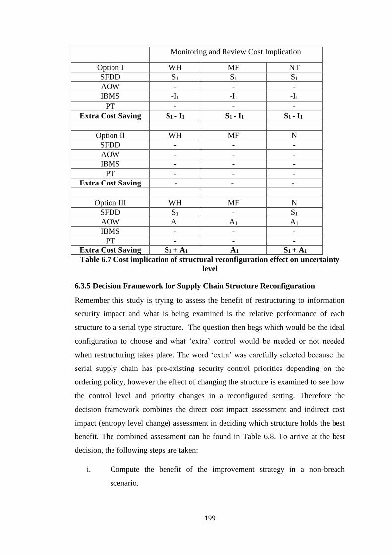
199

Monitoring and Review Cost Implication

Option I WH MF NT

SFDD S1 S1 S1

AOW - - -

IBMS -I1 -I1 -I1

PT - - -

Extra Cost Saving S1 - I1 S1 - I1 S1 - I1

Option II WH MF N

SFDD - - -

AOW - - -

IBMS - - -

PT - - -

Extra Cost Saving - - -

Option III WH MF N

SFDD S1 - S1

AOW A1 A1 A1

IBMS - - -

PT - - -

Extra Cost Saving S1 + A1 A1 S1 + A1

Table 6.7 Cost implication of structural reconfiguration effect on uncertainty

level

6.3.5 Decision Framework for Supply Chain Structure Reconfiguration

Remember this study is trying to assess the benefit of restructuring to information

security impact and what is being examined is the relative performance of each

structure to a serial type structure. The question then begs which would be the ideal

configuration to choose and what ‘extra’ control would be needed or not needed

when restructuring takes place. The word ‘extra’ was carefully selected because the

serial supply chain has pre-existing security control priorities depending on the

ordering policy, however the effect of changing the structure is examined to see how

the control level and priority changes in a reconfigured setting. Therefore the

decision framework combines the direct cost impact assessment and indirect cost

impact (entropy level change) assessment in deciding which structure holds the best

benefit. The combined assessment can be found in Table 6.8. To arrive at the best

decision, the following steps are taken:

i. Compute the benefit of the improvement strategy in a non-breach

scenario.

200

ii. Compute the mitigation benefit of the improvement strategy under

various information security breach scenarios.

iii. Compute the aggregate benefit by adding the improvement benefit in a

non-breach scenario and the various breach scenarios.

iv. Estimate the aggregate cost implication of changing the monitoring and

review level in the supply chain (if cost implication is positive, then it is

considered cost saving benefit; but if cost implication is negative, then it

is considered to be an additional cost).

v. Compute the overall benefit by adding i, ii, iii and iv.

vi. To decide on the ideal configuration the one with the highest cost benefit

is selected

The aggregate structural reconfiguration benefit in a non-breach scenario (n-BS) and

in various breach scenarios (BS) under each ordering policy has been established in

section 5.3.4. This is extracted and included in Table 6.8. A 1% increase or decrease

in benefit is equivalent to £3.97 (for option I); £3.10 (for option II); £3.00 (for option

III).

From Table 6.8, it is clear that, under the parameter based policy, the WH and NT

structures exacerbates the aggregate daily cost performance of the supply chain in

both non-breach and breach scenarios by 3% and 6% respectively while MF

improves it by 4%. Entropy assessment however indicate that the effect of all three

strategies is similar with an implied cost of S1 - I1. Therefore, the MF structure can be

adopted if and only if 4% + S1 is significantly greater than I1. Otherwise the serial

structure is better off than when reconfiguration into any of the structures discussed.

Under the batch ordering system, the supply chain need not worry about changing

the monitoring and review level and the final decision can be based on the direct cost

impact alone. Therefore, having considered the direct and indirect cost implications

of structural reconfiguration, the networking strategy appears to be the best strategy

under normal and disruption circumstances.

With the combined ordering system, structural reconfiguration provides additional

cost savings especially under highly disruptive or highly recurring breach. Since the

wholesaling simplification strategy offers the best performance under the direct

impact assessment and joint best under the indirect cost assessment, it is very clear

201

that WH structure is the ideal reconfiguration choice for the combined batch-and-

parameter ordering system.

Option I WH MF NT

Aggregate benefit (n-BS

and BS) -3% 4% -6%

Monitoring and review

cost

S1 - I1 S1 - I1 S1 - I1

Overall benefit -3% + S1 - I1 4% + S1 - I1 -6% + S1 - I1

Decider Max (WH, MF, N)

Final Decision No reconfiguration, if MF: 4% + S1 >> I1, else MF

Option II WH MF NT

Mitigation benefit 49.8% 47.7% 50.9%

Monitoring cost - - -

Overall benefit 49.8% 47.7% 50.9%

Decider Max (WH , MF, NT)

Final Decision NT

Option III WH MF NT

Mitigation benefit 29.0% 21.7% 25.0%

Monitoring cost S1 + A1 A1 S1 + A1

Overall benefit 29% + S1 + A1 21.7% + A1 25.0% + S1 + A1

Decider Max (WH, MF, NT)

Final Decision WH

1% is equivalent to £3.97 (for option I); £3.10 (for option II); £3.00 (for option III).

Table 6.8 Decision framework for structural reconfiguration under each

ordering policy

6.4 INFORMATION SHARING LEVEL EFFECT ON UNCERTAINTY

LEVEL OF BREACH IMPACT

The result of the rating outcome for information sharing level effect on ordering

systems I, II and III can be found in Appendix 6.2. The aim of this section is to

establish the relative change in entropy level due to adopting various information

sharing strategies and to examine the cost implication to monitoring and review

202

activities. To the end of understanding how this can affect information sharing

adoption decision. An examination of this result in the manner with which section

6.3 was examined will provide the same level of insight for each ISL.

6.4.1 Entropy Analysis of RW Effect

The result of the relative change in uncertainty level due to information sharing

between the retailer and wholesaler only can be found in Table 6.9.

SFDD


option I 0 1 0 0

option II 0 -1 -2 -1

option III 0 0 0 0

AOW


option I 0 -1 0 -1

option II -1 0 -1 0

option III 1 0 0 1

PT


option I 0 -1 1 0

option II 0 0 -1 0

option III 1 -1 0 1

IBMS


option I 0 -1 1 -1

option II 0 0 -1 0

option III 0 0 0 0

Table 6.9 Effect of RW mode on information security breach impact

uncertainty level

Under the parameter based ordering system, information sharing between the retailer

and the wholesaler alone in the supply chain increases the level of breach impact

uncertainty by one under BP1 and BP2. However, under BP3, there is no difference

between the uncertainty level in the non-information sharing mode (NI) and the RW

mode. The uncertainty level remains unchanged for the retailer under all three breach

profiles while that of the wholesaler is increased by one level under BP1 and BP2

but decreased by one level under BP3. The manufacturer only derived a one level

reduction in uncertainty level under BP1 but observed no changes to uncertainty

level under high disruption duration or RoC.

For the batch ordering system, RW effect cause a stabilisation of the uncertainty

level under BP1 and BP2 but increases it under BP1 by one level (from low to

203

medium). For the respective supply agents, the wholesale experience a similar effect

to that of the entire supply chain but the retailer is unaffected except under BP2

where a one level increase is observed. The manufacturer is worst affected with a

one level increase under BP1 and BP2 and a two level increase under BP3. The

manufacturer happens to be the hotspot for uncertainty in such supply chains using

the batch ordering policy.

With the combined policy type, there is an observed one level reduction in

uncertainty level after RW information sharing mode adoption only under BP2. On

the other hand, the manufacturer and wholesaler are unaffected under all three

scenarios while the retailer only benefits under BP1.

6.4.2 Entropy Analysis of WM Effect


between the wholesaler and manufacturer only can be found in Table 6.10.

At the supply chain level, under a parameter based ordering system, adopting the

WM mode of information sharing worsens the uncertainty by a level when the

supply chain faces a breach of BP1 type but there is no apparent effect on the

uncertainty level when the disruption duration and RoC are increased significantly.

However at the level of the individual supply agents, only the manufacturer enjoys a

reduced uncertainty level under BP2 and BP3 while the other agents are unaffected

regardless of the breach profile.

Under the batch ordering policy, the uncertainty level in the supply chain and at each

individual agent is unaffected by a WM configuration. Hence no change in

monitoring and review level required.

With the combined policy, the supply chain uncertainty level is only affected under

PT breach and this is due to the fact that WM mode reduces the entropy level at the

retailer (from low to nil) under this breach. The manufacturer is unperturbed by the

WM mode regardless of the breach profile but the wholesaler is affected negatively

under BP2 with a level increase in uncertainty

.

204

SFDD


option I 0 0 1 0

option II 0 0 0 0

option III 0 0 0 0

AOW


option I 0 0 1 0

option II 0 0 0 0

option III 0 -1 0 0

PT


option I 0 0 0 0

option II 0 0 0 0

option III 1 0 0 1

IBMS


option I 0 0 0 -1

option II 0 0 0 0

option III 1 0 0 0

Table 6.10 Effect of WM mode on information security breach impact

uncertainty level

6.4.3 Entropy Analysis of RWM Effect


between the wholesaler and manufacturer only can be found in Table 6.11.

The effect of full integration on the uncertainty level in a supply chain using

parameter based ordering policy is a one level increase in breach impact uncertainty

when a breach of the type BP1 and BP2 occurs. There is no effect on uncertainty

level when breach of the type BP1 occurs. At the operational level, the wholesaler is

affected in a similar way to the supply chain but the retailer and manufacturer are

unaffected by the full information sharing strategy under any of the breach profiles.

With the batch ordering system, adopting a full information sharing strategy does not

affect uncertainty level when BP1and BP2 occurs but the uncertainty level is

decreased by one level when PT occur. This means that a little increase in the RoC

of the breach (comparing IBMS to PT) reduces the uncertainty level in a fully

integrated mode by one level while a significantly high increase in RoC (comparing

IBMS to AOW) has no effect. On the other hand, the uncertainty level is increased

by a level when the more disruptive breach occurs. Interestingly, the impact

uncertainty at the manufacturer is reduced by a level only under BP1, increased at

205

the wholesaler by a level only under BP3 and increased at the retailer by a level only

under BP2.

RWM SFDD


option I 0 0 0 0

option II 0 -1 0 -1

option III 0 0 0 0

AOW


option I 0 -1 0 -1

option II -1 0 0 0

option III 1 -1 0 0

PT


option I 0 -1 0 -1

option II 0 0 1 1

option III 1 -1 0 0

IBMS


option I 0 -1 0 -1

option II 0 0 1 0

option III 0 0 0 0

Table 6.11 Effect of WM mode on information security breach impact

uncertainty level

Under the combined policy, RWM does not affect the uncertainty at the supply chain

level under any of the breach profiles. At the operational level, the manufacturer is

also unaffected by the full information sharing mode. However the retailer benefits

with a level reduction in uncertainty only under increased RoC while the wholesaler

experiences a level increase in uncertainty under similar conditions.

6.4.4 Summary and Cost Implication of Entropy Change Due to Information

Sharing

The implication of the effect of various information sharing modes on uncertainty

level to monitoring and review control cost is patterned in a similar way to that

described for the structure effect in section 6.3.4. The result in Table 6.12 reveals the

cost implication of engaging in information sharing at the RW, WM and RWM

levels based on the monitoring and review level change required.

206

Monitoring and Review Cost Implication

Option I RW WM RWM

SFDD - - -

AOW -A1 - -A1

IBMS -I1 -I1 -I1

PT - - -P1

Extra Cost Saving -(A1 +I1) -I1 -(A1+P1+I1)

Option II RW WM RWM

SFDD -S1 - -S1

AOW - - -

IBMS - - -

PT - - P1

Extra Cost Saving -S1 - P1-S1

Option III RW WM RWM

SFDD - - -

AOW A1 - -

IBMS - - -

PT P1 P1 -

Extra Cost Saving A1+P1 P1 -

Table 6.12 Cost implication of structural reconfiguration effect on monitoring

and review cost

Under the parameter based ordering, it is clear from the result that there is additional

cost required by the supply chain, where retailer’s information is being shared with

the wholesaler, in order to increase its control over AOW and IBMS information

security breach impact. Including the manufacturer in the sharing of retailer

information increases the monitoring and review cost by P1. Information sharing that

does not involve sharing retailer’s information but that only focuses on sharing

wholesaler information with the manufacturer needs to increase its monitoring level

for IBMS and hence will incur additional cost of monitoring and review. Therefore

with the RW and RWM strategy, total monitoring and review control cost should

increase if the same level of control over security breach impact as that of a non-

integrated supply chain is to be maintained.

With the batch ordering system, sharing retailer’s information with the wholesaler

alone requires an increase in total monitoring and review cost by S1 while including

the manufacturer in this information sharing reduces the S1 cost by providing

additional cost saving of P1. The strategy that only involves sharing wholesaler’s

information with the manufacturer does not incur any additional cost regardless of

the breach profile.

207

Information sharing under the combined batch-and-parameter based ordering policy

does not increase the uncertainty or complexity of the supply chain. The result

suggest that sharing retailer’s information with the wholesaler alone saves

monitoring and review cost (by A1+P1) while extending this information to the

manufacturer will only eliminate this benefit but it would still be at the same level

with that of a non-integrated supply chain. On the other hand, only sharing

wholesaler’s information with the manufacturer helps save monitoring and review

cost by P1.

6.4.5 Decision Framework for Supply Chain Information Sharing Level

Again the final decision of which ISL is most desirable for each ordering policy

should not only be based on the above assessment, as it might be misleading, but

also on the entropy assessment and its implication. Similar to the discussion in

section 6.3.5, this section evaluates the performance of each ISL under various

information security breach at the supply chain level. The decision framework

incorporates the direct mitigation cost benefit of engaging in information sharing at

different levels and the cost associated with uncertainty level change due to security

breach. To decide on the ideal level of information sharing for each ordering policy,

the steps outlined in section 6.3.5 is applied but with information sharing level as

focus instead of supply chain structure. The result of this computation is summarised

in Table 6.13. Recall that 1% is equivalent to £3.97 (for option I); £3.10 (for option

II); £3.00 (for option III).

From the result in Table 6.13, it is clear that under a parameter based ordering

system, the supply chain will have to incur certain costs to increase the level of

control that may otherwise be lost after adopting information sharing strategies.

Based on simple logic, the best information strategy is this case would depend on the

following conditions. If P1 is lesser than 30%, then RWM is the best choice,

otherwise RW will be the best choice. However if A1 is less than 35%, then WM

would become the ideal and if I1 is less than 1%, then a non-integrated scenario

would be the ideal case.

208

Option I RW WM RWM

Aggregate benefit (n-BS

and BS) 36% 1% 66%

Monitoring and review

cost -(A1 +I1) -I1 -(A1+P1+I1)

Overall benefit 36% - (A1 +I1) 1% -I1 66% - (A1+P1+I1)

Decider Max (RW, WM, RWM)

Final Decision RWM (IF P1<30%, Else RW (IF A1< 35%, Else WM (IF

I1<1%, Else No integration)))

Option II RW WM RWM

Mitigation benefit 12% 6% 31%

Monitoring cost -S1 - P1-S1

Overall benefit 12%-S1 6% 31% + P1-S1


Final Decision RWM (IF S1 < P1 + 25%, Else WM)

Option III RW WM RWM

Mitigation benefit 18% 27% 32%

Monitoring cost A1+P1 P1 -

Overall benefit 18% + A1+P1 27% + P1 32%


Final Decision RWM (IF P1<5%, Else WM (IF A1> 9%, Else RW))


Table 6.13 Decision framework for ISL adoption under each ordering policy

For a batch ordering system, the decision is clearly between RWM and WM. If the

cost magnitude of S1 is less than that of P1 + 25%, then the full integration mode

would be the ideal choice for the batch ordering system under these conditions,

otherwise WM would be the preferred choice.

With the combined policy, the decision is a bit more complicated than in the batch

ordering system. The selection would be RWM, provided the magnitude of P1 is less

than 5%, otherwise WM would be favoured. However, if A1 is less than 9%, RW

becomes the best choice.

209

6.5 INFLUENCE OF THE INTERACTION BETWEEN ISL AND

STRUCTURE ON UNCERTAINTY LEVEL OF BREACH IMPACT

The influence of structural reconfiguration and information sharing strategies has

been discussed separately in section 6.3 and 6.4 respectively. However the aim of

this section is to establish how combining the two strategies would affect breach

impact uncertainty and the cost implication of this under the three ordering policies.

Given the proposed indirect cost assessment (entropy assessment), the objective is to

know if combining both improvement strategies would be beneficial to the supply

chain cost performance or if using a single improvement strategy would be better. It

is also aimed to establish whether the decision made from direct cost assessment

alone will be different from that made when the indirect cost assessment has been

included. The result of the entropy level rating of the various combination of

information sharing level (ISL) and supply chain structure scenarios can be found in

Appendix 6.3.

6.5.1 Summary and Cost Implication of Entropy Change Due to the Combined

Effect of Information Sharing and Supply Chain Structure

The change in entropy level as a result of the combined effect is shown in Table 6.14

and the cost implication is shown in Table 6.15. As a general observation from Table

6.14, under the parameter based policy, the effect of information sharing on the

breach impact uncertainty level in different supply chain structures is mostly

negative when the breach is of the BP1 type. The interaction effect is mostly of the

stabilising or improvement type on uncertainty level under BP3 while it is mostly of

a stabilising type under BP2. With the batch ordering policy, the interaction effect is

mostly of the stabilising type under all three breach profiles. For the combined policy

type, the interaction effect is predominantly of the stabilising type under BP1 type

while the effect is predominantly of the improvement type under BP2 and BP3.

Of the three ordering options, it appears that the batch ordering policy is the most

stable to uncertainty level change due to the interaction effect under all three breach

profiles. The combined policy offers the next best stability but the inherent

instability favours the interaction effect under breaches of the type BP2 and BP3.

The parameter based policy is the most unstable of the three to the interaction effect

and this instability does not favour the interaction effect under breaches of type BP1.

210

In terms of the implication to cost, the result in Table 6.15 reveal that the interaction

effect between the structural reconfiguration and information sharing strategies in a

batch ordering system hardly incur additional monitoring and review cost, but the

combined batch-and-parameter ordering policy provide additional cost saving in all

but one of the various combinations. The interaction effect in a parameter based

policy supply chain, however, requires additional monitoring and review cost for

virtually all the combination scenarios.

RW WM RWM

Option I

Breach WH MF NT WH MF NT WH MF NT

SFDD 0 1 0 1 0 1 1 1 0

AOW 0 0 0 -1 -1 0 0 0 0

PT -1 0 -1 0 -1 -1 -1 -1 -1

IBMS -1 -1 -1 -1 -1 -1 -1 -1 -1

Option II


SFDD 0 0 -1 0 0 0 0 0 0

AOW 0 0 0 0 0 0 1 0 1

PT 0 0 0 0 0 0 0 0 0

IBMS 0 0 0 0 0 0 0 0 0

Option III


SFDD 1 1 1 0 0 1 1 1 1

AOW 1 0 1 1 0 1 1 1 1

PT 0 0 0 1 0 0 0 0 0

IBMS 0 0 0 0 0 0 0 0 0

Table 6.14 Relative change in uncertainty level due to ISL and structure

interaction effect

211

RW WM RWM

Option I

Breach WH MF NT WH MF NT WH MF NT

SFDD - S1 - S1 - S1 S1 S1 -

AOW - - - A1- A1- - - - -

PT P1- - P1- - P1- P1- P1- P1- P1-

IBMS I1- I1- I1- I1- I1- I1- I1- I1- I1-

Extra Cost Saving -(P1+I1) -I1 -(P1+I1) S1-A1-I1 -(A1+P1+I1) S1-P1-I1 S1-P1-I1 S1-P1-I1 -(P1+I1)

Option II


SFDD - - S1- - - - - - -

AOW - - - - - - A1 - A1

PT - - - - - - - - -

IBMS - - - - - - - - -

Extra Cost Saving - - -S1 - - - A1 - A1

Option III


SFDD S1 S1 S1 - - S1 S1 S1 S1

AOW A1 - A1 A1- - A1 A1 A1 A1

PT - - - P1 - - - - -

IBMS - - - - - - - - -

Extra Cost Saving S1+A1 S1 S1+A1 A1+P1 - S1+A1 S1+A1 S1+A1 S1+A1

Table 6.15 Cost implication of the interaction effect on monitoring and review cost

212

6.5.2 Decision Framework for Combining Information Sharing and Supply

Chain Structure

To decide on the ideal combination of information sharing level and structure for

each ordering policy, the decision framework incorporates the direct impact

assessment and the indirect impact assessment. Again, the steps outlined in section

6.3.5 are followed. The result of the computation in step (iii) has been established in

section 5.5 and this is added to the cost implication of uncertainty level change

already established in section 6.5.1. The overall benefit is computed and shown in

Table 6.16. Recall that 1% is equivalent to £3.97 (for option I); £3.10 (for option II);

£3.00 (for option III).

RW

WH MF NT

Option I 46.3% -(P1+I1) 45.5% -I1 8.2% -(P1+I1)

Option II 52.9% 63.6% 23.1% - S1

Option III 43.9% + S1+A1 53% + S1 2.7% + S1+A1

WM

WH MF NT

Option I 4.2% +S1-A1-I1 - (1.2% +A1+P1+I1) S1-P1-I1-2.9%

Option II 57.5% 40.3% 51.5%

Option III 67% + A1+P1 39.8% 54.1% + S1+A1

RWM

WH MF NT

Option I S1-P1-I1+87.4% S1-P1-I1+88.4% 44.4% - (P1+I1)

Option II 75% + A1 78.3% 34.1% + A1

Option III 59.7% + S1+A1 61.3% + S1+A1 34.0% + S1+A1

1% is equivalent to £3.97 (for option I); £3.10 (for option II); £3.00 (for option

III).

Table 6.16 Overall Mitigation Benefit under combined strategies

It is clear from the result that given a batch ordering or combined batch-and-

parameter based ordering system, significant benefit can be derived when the retailer

shares its inventory information (including market demand) and even greater benefit

can be derived when this information is shared with the manufacturer. Interestingly,

sharing only the wholesaler information with the manufacturer under similar

ordering policies yields significant overall benefit to the supply chain, even more

than the RW and RWM strategies in some instances. The benefit derived under a

parameter based policy however depends on certain conditions.

213

It is important for supply chains to know, given their pre-existing conditions, how

these two advocated performance improvement strategies can be adopted. For those

pre-existing in certain structures similar to those described in this study, the best

information sharing strategy would be desired. On the other hand, for those who

have already adopted some form of information sharing strategy and would like to

improve the structure of the supply chain would consider the best structural

reconfiguration strategy. This decision, given pre-existing conditions, is explained in

the subsequent sections.

6.5.2.1 Decision for structural reconfiguration given ISL and ordering

Policy

The best combination of structural reconfiguration with existing information sharing

strategy is shown in Table 6.17. For the parameter based ordering policy, decision of

whether to adopt any reconfiguration strategy at all depends on the magnitude of P1

and I1. For a supply chain already adopting RW information strategy, if the

magnitude of P1 and I1 is greater than 46.3% (which is equivalent to £ 183.8), then

the supply chain is best to avoid adopting any of the reconfiguration strategies.

Otherwise manufacturing or wholesaling simplification can be selected depending on

whether P1 is greater than 0.8% (equivalent to £3.2) or not. The decision for

structural reconfiguration in supply chain with pre-existing WM and RWM strategies

is predicated on certain conditions as well.

With the batch ordering and combined policy, the result in Table 6.17 suggests that

structural reconfiguration can be implemented with potential for significant benefit.

The decision of which reconfiguration strategy to select is quite straight forward in

batch ordering system while in a combined policy type, the decision is not straight

forward at least for the partial information sharing strategies (RW and WM).

214


RW

MF (IF P1>0.8%, Else

WH (IF P1+I1<46.3%,

Else No combination )

MF MF (IF A1< 9.1%, Else

WH)

WM

WH (IF A1< P1+7.1%,

Else NT (IF

S1>P1+I1+2.9%, Else No

combination)

WH WH (IF S1<P1+12.9%,

Else NT)

RWM MF (IF P1+I1 < 44.4%,

Else No combination) MF MF


Table 6.17 Structural reconfiguration strategy decision given various ISL

6.5.2.2 Decision for ISL Given Structure and Ordering Policy

The best combination of structural reconfiguration with existing information sharing

strategy is shown in Table 6.18. With the parameter based policy, again, the decision

to adopt any information sharing should be preceded by the examination of certain

conditions and these conditions vary for different supply chain structures. Under the

batch ordering system, the decision of which information sharing best suit the

current structure is quite straight forward for all pre-existing structures, except for

the network structure where the decision is between RWM and WM depending on

the magnitude of A1. For the combined policy type, the decision is also straight

forward except under a wholesaler type structure (WH) where the decision is

between RWM and WM depending on the size of S1 and P1.


WH

RWM (IF P1< 83.2%+A1, Else

WM (IF S1 > 4.2% +A1+I1,

Else No combination)

RWM RWM (IF S1 > 7.3%

+ P1, Else WM)

MF

RWM (IF P1< S1 + 42.9%, Else

RW (IF I1<45.5%, Else No

combination)

RWM RWM

NT

RWM (IF S1< 47.3%, Else

WM (IF S1>P1+I1-2.9%, Else

No combination)

RWM (IF

A1>17.4%, Else

WM)

WM


Table 6.18 Information sharing level strategy decision given various supply

structures

6.5.2.3 Decision for combining ISL and structural reconfiguration

strategy given specific ordering policy

Supply chains seeking to improve their cost performance by adopting both

improvement strategies, given a prevailing ordering policy, will need to decide

215

which combination of structural reconfiguration strategy and information sharing

strategy would be most ideal. The best combination of structural reconfiguration

with information sharing strategy under each ordering policy is shown in Table 6.19.

The decision based on the direct cost assessment in the previous chapter (section 5.6)

was RWM+MF for option I and option II and WM+WH for option III. However

from the entropy assessment, this study has shown that such decisions based on

direct cost assessment alone may, in fact, be misleading.

Best Combination

Option I RWM+MF(IF P1< 92.6%+A1, Else WM+WH (IF A1< S1- 41.3%,

Else RW+MF (IF I1<45.5%, Else No combined adoption)))

Option II RWM+MF (IF A1 <3.3%, Else RWM+WH)

Option III RWM+MF (IF S1> 5.7% + P1, Else WM+WH)


Table 6.19 Decision making for combined ISL and structural reconfiguration

strategy

6.5.2.3 Decision for the overall best ISL, Structure and Ordering Policy

Combination

Through the process of elimination by pairwise comparison one can obtain the

scenario that offers the best combination of ISL, supply chain structure and ordering

policy. It is inaccurate to use the percentage values for direct comparison between all

scenarios because the magnitude of a percentage is different for each ordering

policy. Therefore an accurate and direct comparison would require the use of cost (£)

instead of percentage. It has been established that 1% is equivalent to £3.97 (for

option I); £3.10 (for option II); £3.00 (for option III).

By considering the best options for each ordering policy and substituting the

percentage values with their corresponding pound (£) equivalent, the overall best

combination is selected contingent on the following conditions:

RWM+WH+II (IF P1<£31.5, Else WM+WH+III (IF S1<£7.1+P1, Else

RWM+MF+III (IF A1>£167.05-P1-I1, Else RWM+MF+I (IF S1>P1+I1- £108.22, Else

RWM+MF+II)))).

The decision could be any of the above five combinations depending on the

magnitude of S1, A1, P1 and I1 which are the respective average daily cost of

216

increasing the monitoring and review activities by one level for SFDD, AOW, PT

and IBMS breaches respectively.

6.6 CONCLUSION

Recall that this study is about understanding the impact of information security

breach with the presumption that this cost estimate is in itself uncertain. The study

has shown that predicting this impact can be uncertain and judging only by the

average cost estimate may be misleading. Many organisations do not consider

breaches with low cost impact as worthy of concern but history has shown that what

might seem benign a year ago may become the bane of existence the following year

due to changing complexities or environmental conditions. It is therefore imperative

to understand the uncertainty surrounding the cost estimate so that an organisation

would not be caught unawares. After the 2011 Sony’s PlayStation Network (PSN)

security breach incidence, some experts opined that Sony was not prepared for such

an attack and did not respond to the breach adequately and did not warn their

consumers soon enough (Newman, 2011, Pollack, 2011). One may therefore

presume that had Sony been certain about the huge impact of hacking incidence in

their risk assessment then it might have implemented the right mix of risk prevention

and mitigation strategies or at least increased their level of monitoring and review

control (i.e. correction strategy). This study has therefore proposed measuring this

uncertainty using entropy assessment.

From the entropy assessment, the study found that the impact of information security

breach on supply chains operating with an optimal batch ordering policy is more

stable, hence less control is required when changing strategic elements of the supply

chain than in a supply chain using the combined policy type. Those with the

parameter based ordering system would require additional level of control when

confronting the impact of information security breach.

The study also found that the effect of the strategic factors on the uncertainty level is

similar for the batch policy and the combined policy type when the profile of the

breach is of the less disruptive and less recurring nature (BP1) or highly disruptive

but less recurring (BP3). However, when the profile of the breach is highly increased

in terms of the breach recurrence rate (as in BP2), this effect is dissimilar with the

217

combined policy parameter enjoying better stability and hence offering better

control.

In terms of the cost implication of uncertainty level change, the results suggest that

the interaction effect between the structural reconfiguration and information sharing

strategies in a batch ordering system hardly incur any additional monitoring and

review cost, but the combined batch-and-parameter ordering policy provide

additional cost saving in virtually all the various combinations. On the other hand,

the interaction effect in a parameter based policy requires additional monitoring and

review cost in the supply chain for virtually all scenarios.

This study has shown that the decision to undertake restructuring given an ISL or the

decision to engage in information sharing given a particular structure is not straight

forward from the initial impact cost assessment. Hence the conditions for decision

has been shown in the framework for deciding ISL or supply chain structure for each

ordering policy and for deciding ordering policy for each ISL and Structure

combinations. The overall best supply chain state (i.e. ISL+ Structure+ Ordering

option) has been shown and this depends on the magnitude of the cost implications

of the various information security breaches. In conclusion, upon impact uncertainty

consideration using entropy assessment, the study has shown that the cost associated

with the impact uncertainty could make, what was otherwise thought of as a good

decision into a wrong one.

218

Chapter 7 : IMPLICATION AND CONCLUSION OF FINDINGS

Information security breach is increasingly becoming a huge subject in supply chain

management owing to the increased level of dependence on information systems and

the increased level of interdependence between operating partners brought about by

integrated information systems. Several threats to information security exist that can

compromise the confidentiality, integrity and availability of the goods and/or

services provided by organisations. Therefore information security breach impact

assessment is strongly advocated for a compromise to the information system may

have restrictions on the flow of information, which may ultimately disrupt the flow

of material in the supply chain. This has been shown to have catastrophic impact on

the cost performance as well as the service performance of supply chain agents.

To understand the landscape of information security impact and the role certain

supply chain strategic factors play in this impact, this research was divided into three

separate studies. The first study (Chapter 4) was to understand the improvements in

supply chain performance that can be derived, under normal circumstances (i.e. no

information security breach), when those strategic factors are changed from one

alternative to another. This also serves as the bench mark for estimating the impact

of information security breach. The second study (Chapter 5) examined the impact of

information security breach on supply chain performance and how each of these

strategic factors fare in the face of these breaches. The third study (Chapter 6)

established the uncertainty associated with the impact of each security breach using

entropy theory and the implication of this to the monitoring and review level

required in the supply chain. This represented an indirect cost impact assessment

which was used in a final decision framework to guide improvement strategy

adoption decisions.

In the following sections, the main research findings of three studies will be

summarized respectively and the managerial implications of the findings will then be

discussed. It is followed with the research contributions. Finally, a critical discussion

of limitations is provided before the future research directions are pointed out.

219


1

7.1.1 The Role of Ordering Policy in a Non-Breach Scenario

7.1.1.1 Effect on Ordering Pattern

Given similar operating conditions, the magnitude of the order quantity each time an

order is placed is higher in a batch ordering policy than in a parameter based

ordering policy. Consequently, the frequency of ordering in the former is less than

that of the latter. The cost performance of the batch ordering system was better than

that of the parameter based ordering suggesting that the ordering pattern (magnitude

of order quantity and the frequency of ordering) of the former was more favourable

to supply performance than the latter. However, the ordering pattern of an ordering

policy which combines aspects of the batch ordering system and parameter based

ordering was the median of the three and the performance under this combined

policy was the highest of all three ordering policies. This indicates that there exists a

point along the ordering pattern continuum between batch ordering and parameter

based ordering where performance is optimal (or at least near optimal). Therefore the

combined policy appears to be an improvement of the batch ordering and the

parameter based ordering and can be considered to be an ordering policy

improvement strategy. The same result was observed under all three supply

structures which validates the findings.

Managerial Implication: Certain supply chains favour certain shipping strategies

depending on whether bulk purchase is made less frequently or whether smaller

quantities are needed to be shipped more frequently. The optimal EOQ ordering type

would require a shipping strategy that favours higher order quantity with less

ordering frequency while a base stock policy under the same supply chain condition

would require a shipping strategy that favours lower order quantities ordered more

frequently.

7.1.1.2 Effect on Bullwhip

The bullwhip effect has been the subject of many articles on supply chain

management. Several authors have examined the factors that contribute to an

increase in the bullwhip effect while others have suggested improvement strategies.

However this study supports the earlier contribution of Chen and Samroengraja

220

(2004) and has shown that incorporating strategies to reduce the bullwhip effect does

not necessarily constitute improvement in supply chain cost performance. In fact, as

the results suggest, the policy with the lowest bullwhip effect (option I- parameter

based ordering policy) has higher supply chain cost than that with higher bullwhip

effect (option II- batch ordering policy). This study also included the wholesaler tier

in the simulation modelling, which was not included in the work of Chen and

Samroengraja (2004) when they made that assertion, and found evidence to support

the claim of Baganha and Cohen (1998) that the wholesaler has a stabilising effect

on bullwhip effect. However this claim of the stabilising role of the wholesaler does

not always apply, at least, to the combined batch-and-parameter based policy type

(option III).

Managerial Implication: The implication of the bullwhip effect from past literature

is that upstream agents tend to carry excess inventory and therefore incur higher

inventory holding cost. Part of the strategies of reducing the bullwhip effect could be

introducing a wholesaler which could effectively be a sort of distribution center

acting autonomously. Again this has to be justified by analysing the cost of having

such a structure against the reduction in inventory and other associated costs that it

will generate.

7.1.2 The Role of Structural Reconfiguration in a Non-Breach Scenario


Structural reconfiguration as a strategy does not affect the ordering pattern of a

parameter based policy but affects that of batch and combined batch-and-parameter

based ordering by reducing the effective average order quantity (EAOQ) and a

commensurate increase in ordering rate (OR). Consequently, the cost performance in

a parameter based ordering system does not change while the cost performance in

the other two ordering policies is improved by any of the three structural

reconfiguration strategies considered. It is clear that simplifying the ‘deliver’ aspect

of the supply chain (i.e. the wholesaler tier) is the best option for a combined policy

type while simplifying the ‘make’ aspect (i.e. the manufacturer tier) is the best

choice of structural reconfiguration for a supply chain using a batch ordering policy.

Managerial implication: Therefore one can infer that supply chains using the

parameter based policy (base stock policy) need not change their shipping strategy

221

when considering structural reconfiguration, but those using batch or combined

batch-and-parameter based models should revisit their shipping strategy to adopt one

that favours lesser order quantity placed more frequently. In addition, changing the

structure of a supply chain can be difficult especially for those organisations in

existing serial structures. For a supply chain using batch ordering policy (e.g.

optimal EOQ model) who wants to derive the benefit of structural reconfiguration

but does not want to go through the hassle of restructuring should consider only

modifying its policy to the combined batch-and-parameter based policy to reap

similar benefits. Therefore the combined policy can be used as a supply chain

performance improvement strategy.

7.1.2.2 Effect on Cost Performance

This study has shown that, like all improvement strategies, structural reconfiguration

does not benefit all the parties in the supply chain and incentives need to be given to

participating agents who are not benefiting from it. Hence a decision framework for

accepting a given improvement strategy is developed and shown in Figure 4.1.

Managerial Implication: For the parameter based policies such as the base stock

policy, again neither simplification nor networking strategies offer any significant

benefit to the supply chain, hence adopting either of these strategies is basically

futile. For batch ordering policies such as the optimal EOQ model, the better strategy

would be to share the orders between agents of the same tier rather than simplify the

supply chain at either the wholesaler or the manufacture tiers, although the latter

strategy still holds benefit. With the combined policy type such as the modified base

stock policy with EOQ component, the preferred strategy is the simplification

strategy at the wholesaler tier rather than networking strategy.

7.1.3 The Role of Information Sharing Level in a Non-Breach Scenario


The general effect of information sharing on the ordering pattern of the supply chain

agents using the shared information is an increase in the effective average order

quantity (EAOQ) and a commensurate increase in ordering rate (OR). This is

contrary to the effect of structural reconfiguration where the case is the other way

round. The ordering pattern of all supply agents using the parameter based policy is

not perturbed by any of the information sharing strategies but under the other two

222

policies, only the retailer’s ordering pattern is not affected by all three information

sharing modes.

Managerial Implication: Therefore, under the batch or combined batch-and-

parameter based models, users of downstream inventory information should revisit

their shipping strategy to adopt one that favours more order quantity placed less

frequently while supply chains using the parameter based policy (base stock policy)

need not change their shipping strategy when considering information sharing at any

level.

7.1.3.2 Effect on Bullwhip

From the control theory perspective, engaging in information sharing does not

change the nature of bullwhip effect for options I and II but only changes the

magnitude. The stabilising effect of the wholesaler is more pronounced when the

wholesaler using a batch ordering policy (e.g. optimal EOQ model) or a combined

batch-and-parameter based ordering (e.g. modified base stock policy) is privy to, and

uses, actual demand information.

Managerial Implication: The supply chain would be able to reduce the bullwhip

effect even further when a wholesaler type entity is introduced and retailer’s

information is shared with at least the wholesaler.

7.1.3.3 Effect on Cost Performance

At the supply chain level, a supply chain using parameter based policy such as the

base stock policy only benefits from information sharing when the wholesaler and/or

the manufacturer uses retailer’s inventory information (which includes the market

demand information). However the supply chain obtains benefit regardless of the

mode of information sharing (RW, WM or RWM) under a batch or combined batch-

and-parameter based ordering policy. Interestingly, RW and RWM favours the

parameter based ordering policy more than the other two policies while WM mode

favours the combined policy more.

Managerial Implication: The partial information sharing strategy that involves

sharing retailer’s inventory information (RW) can be adopted in parameter based and

batch ordering systems without any consideration for giving incentives to non-

benefiting members. However, in the combined policy type system, such information

sharing strategy can still be adopted but the responsibility of incentive giving lies

223

with the manufacturer. On the other hand, the partial information sharing strategy

that does not involve sharing retailer’s information but instead involves sharing

wholesaler information with the manufacturer (WM) is not likely to be acceptable by

the retailer and wholesaler. This is because the overall benefit of the strategy is not

large enough to incentivise both the retailer and wholesaler in a parameter based

system while the manufacturer would have to incentivise both downstream agents

under the batch and combined batch-and-parameter systems for such strategy to be

acceptable. The full information sharing mode (also referred to as full integration in

this study) is completely acceptable by all supply chain agents and no incentivisation

is required under parameter based and batch ordering policies respectively. However,

under the combined policy, the retailer and wholesaler are less inclined to adopt

RWM strategy unless the manufacturer can provide certain incentives to justify their

involvement.


Reconfiguration in a Non-Breach Scenario

This study has shown that the best improvement strategy under the information

sharing category and that under the structural reconfiguration strategy category does

not necessarily have the best synergy performance. Hence, the decision to adopt one

single strategy should be made with a long term view (i.e. strategic) that includes the

possibility of adopting another improvement strategy from a different improvement

category, even if the other improvement strategy would be considered much later in

the future.

Managerial Implication: Therefore the supply chain using the parameter based

policy such as the base stock policy will do well to adopt full information sharing

and manufacturing simplification strategies even if a stepwise adoption is

considered. Clearly for the batch ordering policy such as the optimal EOQ model,

although the individual best performance comes under networking and full

integration separately, the best option on the long run would be the combination of

manufacturing simplification and full integration strategies. Under the combined

policy mode, the decision would be to adopt both wholesaling simplification and

information sharing between the wholesaler and the manufacturer only as opposed to

the full information sharing strategy.

224


2

The second study has shown that the magnitude and direction of breach impact

would depend on the breach profile, and the type of ordering policy being used in the

supply chain. However the magnitude would depend on the current structure and

information sharing level in the supply chain. On another level, this study has

demonstrated that the impact of information security breach, however, can be

mitigated by improvement strategies such as supply reconfiguration and information

sharing as shown in this study. The impact of security breach is significant enough to

affect supply chain decisions with regards to information sharing level (ISL) choice

or supply chain structure preference and it has been established that the decision to

opt for certain ISL and structure combinations should not be taken without

disruption impact considerations.

7.2.1 The Role of Ordering Policy in a Breach Scenario

7.2.1.1 Effect on Breach Impact Resilience

The parameter based policy is the most resilient to the negative impact of a breach,

while the batch ordering policy is the least resilient with the combined policy having

the median resilience. On the other hand, priorities of information security

management can be known when the breach is profiled according to the average

disruption duration and the average rate of occurrence rate. These priorities would

differ based on the ordering policy of choice.

Managerial Implication: Therefore, for a parameter based ordering policy, increased

RoC only increases the oddly positive effect of a breach on the performance while

disruption duration increases the negative effect. Therefore supply chain priority for

such parameter based ordering policy would be to focus on reducing the disruption

duration of a breach, hence breach correction or mitigation would be a priority. The

priority for a supply chain with batch ordering policy and that for a combined batch-

and-parameter based ordering is also breach mitigation as disruption duration had a

greater negative effect on breach cost impact than RoC.

7.2.1.2 The Reverberating Effect

The reverberating effect of the breach impact depends on the ordering policy of

choice. The effect consistently increases under the parameter based policy while the

225

effect consistently decreases under the batch ordering policy. Under the combined

policy the effect increases but the stabilising effect of the wholesaler makes it

decrease as it gets to the manufacturer.

Managerial Implication: Therefore supply chains using the parameter based

ordering should be more wary of information security breach occurring downstream

in the supply chain than those using batch ordering policy. In a supply chain using

the combined policy type, the wholesalers specifically should be wary of information

security breach occurring downstream. This study therefore calls for better

cooperation among supply partners and supports the claim that information security

breach (ISB) incidence should be shared between supply chain partners. This is so

that upstream parties can be made aware of the incidence of the breach early enough

to find ways to eliminate or reduce the reverberating effect of such a breach.

7.2.2 The Role of Structural Reconfiguration in a Breach Scenario

7.2.2.1 Structural Reconfiguration as a Breach Impact Mitigation

Strategy

This section examined the effect of changing the structure of a supply chain from a

serial structure configuration to any of the three structural configurations discussed

earlier. It evaluated the performance of these three structures relative to what would

have been obtained in the serial counterpart. Since these three structures are forms of

simplifying the supply chain by reducing the number of agents at the wholesaler tier

(WH structure) or at the manufacturer tier (MF structure) or by simply risk pooling

(NT structure), this study has shown that reconfiguration to these structure types can

be a worthwhile strategy that can help the supply chain improve cost performance

and also reduce the impact of information security breach. A single-strategy decision

framework that incorporates breach impact assessment was developed and shown in

Figure 5.2.

Managerial Implication: Structural reconfiguration by itself does not mitigate the

impact information security breach has on supply chain performance for a parameter

based policy but instead makes it worse. The only exception is the MF structure

where benefit is derivable and the retailer needs to share ISB incidence and data with

the wholesaler. Reconfiguration will prove beneficial to batch ordering systems and

batch-and parameter based policy in a security breach scenario and there is no need

226

for ISB data sharing and incentivisation after a security breach. In general,

information security management (ISM) priority would be to focus more on

prevention and deterrence when any of the structural reconfiguration strategies is

adopted.

7.2.3 The Role of Information Sharing Level in a Breach Scenario

The performance of a partially or fully integrated supply chain under information

security breach is significantly better than the performance of a non-integrated

supply chain under similar conditions. In general, the full integration mode (RWM)

is the preferable sharing mode regardless of the type of ordering policy be it

parameter based or batch ordering or the combination of both. However, the profile

of the breach affects the performance of each information sharing strategy and some

strategies fare better under certain profiles than others.

Managerial Implication: Apart from the normal incentivisation required in a non-

breach scenario, the study suggest that additional incentivisation for the

reverberating effect of the breach is required for the wholesaler when the sharing

mode does not include sharing the retailer’s information under a parameter based or

combined parameter based ordering policy. However, under the batch ordering

system, further incentivisation and ISB sharing can be prevented when the partial

information sharing strategy of type RW includes the manufacturer in information

sharing.


Reconfiguration in a Breach Scenario

The supply chain stands to benefit from a significant improvement in performance

when these two strategies are used as long as the use and adoption is well informed.

The study has highlighted the best information strategy given a specific supply chain

structure and also the best structural reconfiguration strategy given a specific

information sharing level that may be pre-existing in the supply chain. It has been

shown that certain strategies fare better alone while others that are otherwise

detrimental may yet prove beneficial when combined with other strategies.

Managerial Implication: These two improvement strategies could be used as part of

breach impact management strategy in addition to the ISM measures as they reduce

227

the impact information security breach would otherwise have on a normal serial

supply chain without information sharing.


3

To decide on the ideal configuration for each ordering policy, first the benefit of the

improvement strategy is assessed under a non-breach scenario (n-BS). Then the

performance under various information security breaches is evaluated and the best

improvement strategy is selected based on the aggregate performance in a non-

breach and in various breach scenarios. This aggregate performance is considered to

be the potential benefit held by such an improvement strategy.

However since the impact of information security breach is uncertain in itself,

organisations ought to be wary of this uncertainty and should be intentional about

reducing it. The more certain you are of a negative impact the more convinced you

are that a risk management strategy is needed. However the less certain you are the

less convinced you are on implementing any risk management action which could be

unwise in the long run. According to a 2002 survey by Mitroff and Alpaslan (2003),

proactive businesses existed for an average 16yrs more than their reactive

counterpart. This is perhaps due to the fact that the reactive ones were not certain of

experiencing negative impact and therefore were not proactive about putting proper

mitigation strategy in place. It is therefore of the essence to increase the certainty

level of breach impact so that the necessary corrections or implementation can be put

in place to avoid unprecedented future impact. Increasing the certainty level requires

regular monitoring of the breaches and regular review of the supply chain. This

knowledge of uncertainty is important in the supply chain as according to Mitroff

and Alpaslan (2003) in Altay and Ramirez (2010), 95 percent of Fortune 500

companies are unlikely to be able to manage a disruption that the company has not

experienced before because they are ill-equipped. This could be the bane of

existence for most supply partners.

Reducing the uncertainty level requires actions that are appropriate to the uncertainty

level. These actions involve increasing the level of information required to manage

the supply chain and information security management effectively and be

categorised as monitoring and review control measures. Several monitoring and

228

review activities or measures exist and any organisation cannot implement all of it

but implementation must be guided by the level of control required by the specific

organisation or supply chain.

In addition to the above argument this study also found that, of the three ordering

options, it appears that the batch ordering policy is the most stable to the interaction

effect under all three breach profiles in terms of uncertainty level change. The

combined policy offers the next best stability but the inherent instability favours the

interaction effect under breaches of the type BP2 and BP3. The parameter based

policy is the most unstable of the three to the interaction effect and this instability

does not favour the interaction effect under breaches of type BP1.

Managerial Implication: In terms of the implication to cost, the interaction effect

between the structural reconfiguration and information sharing strategies in a batch

ordering system hardly incur additional monitoring and review cost, but the

combined batch-and-parameter ordering policy provide additional cost saving in all

but one of the various combinations. The interaction effect in a parameter based

policy supply chain, however, requires additional monitoring and review cost for

virtually all the combination scenarios.

The study has shown that, given a batch ordering or combined batch-and-parameter

based ordering system, significant benefit can be derived when the retailer shares its

inventory information (including market demand) and even greater benefit can be

derived when this information is shared with the manufacturer. Interestingly, sharing

only the wholesaler information with the manufacturer under similar ordering

policies yields significant overall benefit to the supply chain, even more than the RW

and RWM strategies in some instances. The benefit derived under a parameter based

policy however depends on the magnitude of a level change in the daily average

monitoring and review cost of the various breaches.

7.5 SUMMARY OF THE RESEARCH CONTRIBUTION

This study examined the impact of various information security breach types on

different supply chain scenarios. An examination of this impact with a focus on the

role that supply chain structure, information sharing level and ordering policy play,

in either mitigating or exacerbating it, is of significance to theory and practice. Not

229

only that, the notion of uncertainty of breach impact makes some organisations wary

of investing in Information System Security. This study therefore applied the

concept of entropy in measuring this uncertainty to guide organisations on how

much investment to make and where the investment is needed most (i.e. priority), if

at all it is required. This study was extensive to a level that has not been done before

in past literature and provided some valuable insight that has significant managerial

implications.

7.5.1 Theoretical Contribution

Theoretically, this study has extended the contribution of a few authors in the distinct

fields of Supply Chain Management and Information Security Management. In the

field of Supply Chain Management, this study extends the works of Hosoda and

Disney (2004) and Chen and Samroengraja (2004) on the effect of ordering policy;

Lau et al. (2002 and 2004) and Wu and Cheng (2008) on the impact of information

sharing; and Beamon and Chen (2001) on the performance analysis of co-joined

supply chain structure on supply chain performance, by examining the synergic

impact of the various combinations of these strategic factors. The study found that

the combination of the various alternatives of each strategic factor have varying

effect on supply chain performance and the best alternative of one factor may not

provide the best benefit when combined with the best alternative of another factor.

Hence a long term perspective should be adopted in these decisions. However, a step

wise adoption can still be done provided the alternatives represent the best

combination on the long run.

In the Information Security Management field, this study appears to represent the

first (if not the only) study in literature that quantified information security breach

impact on supply chain inventory cost performance using the disruption duration and

frequency of breach occurrence information. This study also extends the work of

Whitman (2003) by not only using the frequency of breach occurrence but also

including disruption duration in profiling information security breaches.

7.5.2 Methodological Contribution

A major contribution of this study, in terms of methodology, is the novel application

of Shannon’s Entropy (Shannon 1948) to information security breach impact

assessment. Improvement strategies, while enhancing the cost performance of the

230

organisation or supply chain, may increase the complexity of the operation and

hence make the impact of disruptions even more uncertain. Therefore this study has

shown that the cost benefit of such improvement strategies should be weighed

against the level of uncertainty introduced into the system. It has been established

that a change in the uncertainty level has cost implication and it is important to

include this indirect cost assessment in supply chain strategy decision making.

Hence a simulation-entropy assessment methodology has been developed and

presented in this study to help assess the direct and indirect cost impact of

information security breach which is useful in evaluating any improvement

strategies. The proposed methodology creates a more inclusive approach to impact

assessment than other existing ones that only concentrate on the direct impact such

as Bellefeuille (2005). This can also be applied to the assessment of other types of

threat to supply chain operations. It can also be used to evaluate any strategic

decision aimed at improving supply chain performance. The single-strategy and a

joint-strategy adoption decision framework developed can be used to guide supply

chain management decisions. The joint-strategy framework can be used particularly

for understanding the counter-intuitiveness of combining two or more strategic

decisions.

7.5.3 Contribution to Practice

In the budding field of Supply Chain Response to Information Security, this thesis is

one of the pioneering works to study the influence of various supply chain based

strategic factors such as ordering policy, information sharing level and supply chain

structure on the level of impact information security breach can have on supply chain

performance. In addition, this study has established that synergic effect of these

strategic factors can be used as an information security breach impact mitigation

strategy. This of course should not, in any way, become a substitute for the

implementation of proper security control measures. Their use would however

provide additional benefit that may offset the installation and running cost of

appropriate security controls.

This study also has implication to organisations or supply chains that are interested

in selecting third party security provider or those requiring the services of third party

database or application hosting. Using a third party operator (TPO) takes the

responsibility of IT or IT security away from the organisation or supply chain. It is

231

therefore advisable for organizations to select TPOs based on their security

performance profile as evidenced by their historical performance in providing

adequate security. This requires an assessment of their past and current ability to

prevent security breach from occurring and on how quickly they are able to correct

and restore the functionality of the system after experiencing a compromise. This

assessment can be carried out by profiling the security threats facing the TPO and

this can be done by asking the TPO for information relating to the history of security

breach incidence that has occurred in the past. The security profile of such operators

can be classified as BP1, BP2 or BP3 as shown in this study and this can be used as a

performance criterion in third party service provider selection. This study has shown

that organisations or supply chains should be wary of third party service providers

with history of higher disruption duration profile than those with higher breach

recurrence rate profile. In addition, the level and type of information required in

managing and controlling the system would differ based on the security profile of the

third party operator. Those with high disruption duration profile would worry more

about the extent of negative impact when a breach occurs and those with high breach

recurrence rate would worry more about the impact being negative or positive.

7.6 LIMITATIONS OF RESEARCH

This study would be incomplete if some of the limitations of this study are not

mentioned. Every study has its limitations and this study is without a fair share of

such limitations. One of the main draw backs of this study is that the assessment of

information security breach is only based on four breach types. In practice a lot more

breach types exist and organisations need to make an assessment of all the breach

types they are exposed to. Having said that, this study has allowed for certain level

of generalisability by examining the effect of the breach profile under high and low

states and any organisation can anticipate what the impact of any unconsidered

breach would be as long as the profile is known.

The focus of this study was on the benefit derived from changing the strategic factors

from one alternative to another and does not include a consideration of the cost

required to make such a change. The study agrees that a cost benefit analysis which

compares the cost of implementing improvement initiatives against the benefit that is

derivable is crucial to any acceptance decision. However, the assumption that

232

changing the structure or the ordering policy does not carry huge costs, is not

farfetched. On the other hand, information integration may require substantial capital

but it has been established that computing models such as cloud computing makes

this cost relatively small. Given the peculiarity of supply chains, still this study

believes the onus of decision falls on the supply chain manager after a careful

consideration of the cost of such improvement initiatives against the benefits

established in this study.

Another drawback in this study was the assumption made when a breach occurs. It

was assumed that a customer’s order is not lost and hence the customer will wait for

the system to be restored and then place his order. While this may not be the reality

for some organisations in the fast moving goods (FMG) industry, it is still applicable

in some specialised markets with highly customised product. It can even be argued

that based on the work of Capraro et al. (2003) and Hennig-Thurau and Klee (1997)

it is understood that loyal customers are still likely to purchase from vendors despite

incessant dissatisfaction. In the same line, it was assumed that the demand during the

disruption period is zero and this may affect the forecast estimate especially when

the disruption duration is very high. While the author believes that such an

assumption may affect the breach impact outcome, the effect will not be felt when

the moving average is estimated over a very long period of time. In other words, as

the number of periods increases, the effect of that assumption decreases.

While the ordering policies used may not be the optimal for each scenario, it is

important to state that these policies are frequently used in practice. In addition, this

study does not in any way claim that the forecasting technique used (i.e. Moving

Average Technique) is optimal but it is quite frequently used in practice and

commonly studied. Hence its use is somewhat justified.

The overarching issue of simulation studies is the question of fitness for purpose

(Shannon 1998). Therefore despite some of the above listed limitations, which have

been somewhat justified, the simulation model used in this study is fit for the

purpose for which it was built. The supply chain has been modelled in a similar way

to established supply chain operations and the input parameters used were adapted

from established literature, Lau et al. (2002 and 2004). The output of the experiments

were verified and validated. Although the simulation model assumptions may affect

233

the generalisability of the study, a sensitivity analysis of the models to increased

demand variation shows that only the magnitude of the impact is affected, not the

direction of the impact. Therefore the findings can be generalized to a reasonable

extent.

7.7 FUTURE RESEARCH

There are various types and causes of information disruption (perturbation) that can

occur in the supply chain/network. There is however a need for systematic

classification of information threats and how these threats impact the entire network.

Although some classification of threat exist emanating from surveys done by

practitioners (Baker et al., 2010, Potter and Beard, 2012); institutions (Stoneburner et

al., 2002, Richardson, (2009)) and; academic sources (Samy et al., 2010, Warren,

2000, Whitman, 2003, Loch et al., 1992, Kim et al., 2011), these are partial lists and

there is need for a complete list of threats to information and how these impact the

network and how the supply chain context can be leveraged to contain these impacts.

It is therefore essential to have a systematic and in-depth investigation into the

impact of Information Management on network operations and collaboration

success. To set the ball rolling, this study has proposed a simulation-entropy

assessment approach to investigate the impact of established threats to information

flow on the performance of supply chain and how supply chain contextual factors

moderate these impacts.

Using appropriate case studies or interviews, the cost-benefit analysis should be

carried out for different supply chains in a future study to further substantiate the use

of the approach discussed in this study.

The contextual factors referred to in this study are the structure of the supply chain,

level of integration and ordering policy. These factors, among other complexity

drivers, have more alternatives that require evaluation to build a more holistic picture

of the role of context in supply chain studies.

The impact of assuming zero demand during the breach disruption period would be

investigated under varying forecasting techniques. The forecasting technique

generally requires an estimation of future demand based on the actual demand from

past period. |However, the number of past period demand used in this estimation

234

may vary for different organisations and it is believed that this will affect the impact

of information security breach when the demand during the disruption period is

assumed to be zero. The future study should also investigate the effect of using other

assumptions apart from the zero demand assumption during the disruption duration.

An example is the presumption that demand during the disruption period is same as

that of the last non-zero demand or that it is the average demand over a selected

number of past periods.

235

APPENDIX 4.1 SIMULATION OUTPUT OF ALL THE EXPERIMENTED SCENARIOS

Average cost performance of all the scenarios for options I, II and III.

H-Holding Cost; B- Backlog cost; O- Ordering cost.

Option I


H (£) B (£) O (£) Total (£) H (£) B (£) O (£) Total (£) H (£) B (£) O (£) Total (£) Total (£)

NI-S 0.0 140.0 54.8 194.9 1.9 56.0 54.8 112.7 24.7 5.1 59.6 89.4 397.0

NI-WH 0.0 144.1 54.9 199.0 0.5 59.6 52.4 112.4 21.9 3.0 59.7 84.7 396.1

NI-MF 0.0 139.8 54.9 194.8 1.8 55.3 54.9 112.0 21.8 3.0 54.7 79.5 386.3

NI-NT 0.0 144.0 54.9 198.9 0.5 59.5 54.9 114.9 21.9 3.1 59.7 84.8 398.6

RW-S 0.1 116.4 54.8 171.3 5.2 32.2 54.8 92.3 5.7 26.7 59.7 92.2 355.8

RW-WH 0.1 116.4 54.9 171.4 2.5 31.8 52.4 86.7 3.5 26.6 59.8 89.9 348.1

RW-MF 0.1 116.3 54.9 171.2 4.8 31.6 54.9 91.3 3.5 26.4 54.8 84.8 347.4

RW-NT 0.0 129.3 54.9 184.2 6.5 44.7 54.9 106.1 3.6 26.6 59.8 90.1 380.4

WM-S 0.0 143.9 54.8 198.7 1.7 59.8 54.8 116.2 8.2 9.6 59.8 77.5 392.5

WM-WH 0.0 145.6 54.9 200.6 0.4 61.1 52.4 113.9 9.1 4.7 59.9 73.7 388.2

WM-MF 0.0 145.3 54.9 200.2 1.6 60.7 54.9 117.1 4.5 9.3 54.9 68.7 386.0

WM-NT 0.0 147.1 54.9 202.1 0.5 62.6 54.9 118.0 6.3 6.5 59.9 72.7 392.7

RWM-S 0.1 100.7 54.8 155.6 7.7 16.3 54.8 78.8 17.7 2.2 59.8 79.6 314.0

RWM-WH 0.1 98.2 54.9 153.2 4.6 13.4 52.4 70.4 19.2 1.0 59.9 80.0 303.6

RWM-MF 0.1 100.9 54.9 155.9 7.5 16.0 54.9 78.5 13.2 1.5 54.9 69.6 304.0

RWM-NT 0.0 114.4 54.9 169.3 9.5 29.7 54.9 94.1 15.4 1.1 59.9 76.3 339.8

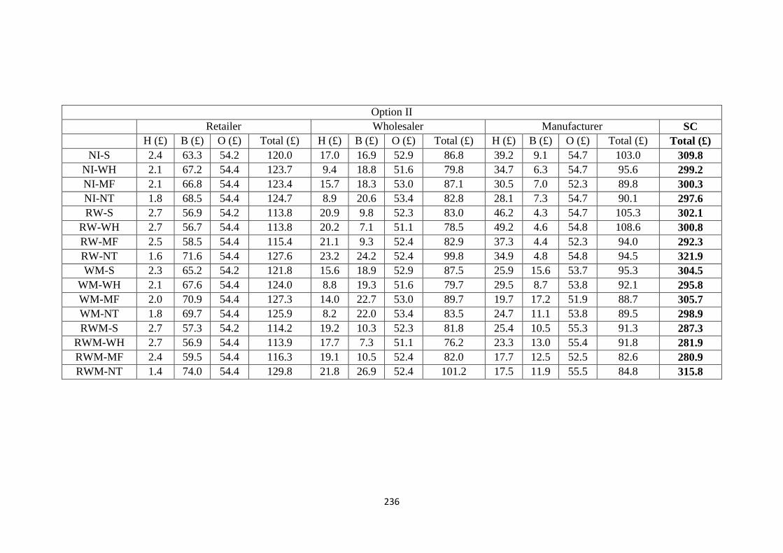
236

Option II



NI-S 2.4 63.3 54.2 120.0 17.0 16.9 52.9 86.8 39.2 9.1 54.7 103.0 309.8

NI-WH 2.1 67.2 54.4 123.7 9.4 18.8 51.6 79.8 34.7 6.3 54.7 95.6 299.2

NI-MF 2.1 66.8 54.4 123.4 15.7 18.3 53.0 87.1 30.5 7.0 52.3 89.8 300.3

NI-NT 1.8 68.5 54.4 124.7 8.9 20.6 53.4 82.8 28.1 7.3 54.7 90.1 297.6

RW-S 2.7 56.9 54.2 113.8 20.9 9.8 52.3 83.0 46.2 4.3 54.7 105.3 302.1

RW-WH 2.7 56.7 54.4 113.8 20.2 7.1 51.1 78.5 49.2 4.6 54.8 108.6 300.8

RW-MF 2.5 58.5 54.4 115.4 21.1 9.3 52.4 82.9 37.3 4.4 52.3 94.0 292.3

RW-NT 1.6 71.6 54.4 127.6 23.2 24.2 52.4 99.8 34.9 4.8 54.8 94.5 321.9

WM-S 2.3 65.2 54.2 121.8 15.6 18.9 52.9 87.5 25.9 15.6 53.7 95.3 304.5

WM-WH 2.1 67.6 54.4 124.0 8.8 19.3 51.6 79.7 29.5 8.7 53.8 92.1 295.8

WM-MF 2.0 70.9 54.4 127.3 14.0 22.7 53.0 89.7 19.7 17.2 51.9 88.7 305.7

WM-NT 1.8 69.7 54.4 125.9 8.2 22.0 53.4 83.5 24.7 11.1 53.8 89.5 298.9

RWM-S 2.7 57.3 54.2 114.2 19.2 10.3 52.3 81.8 25.4 10.5 55.3 91.3 287.3

RWM-WH 2.7 56.9 54.4 113.9 17.7 7.3 51.1 76.2 23.3 13.0 55.4 91.8 281.9

RWM-MF 2.4 59.5 54.4 116.3 19.1 10.5 52.4 82.0 17.7 12.5 52.5 82.6 280.9

RWM-NT 1.4 74.0 54.4 129.8 21.8 26.9 52.4 101.2 17.5 11.9 55.5 84.8 315.8

237

Option III



NI-S 1.9 50.0 54.7 106.7 12.9 12.6 54.3 79.7 56.6 0.6 56.3 113.5 299.9

NI-WH 1.8 48.6 54.8 105.3 8.0 10.4 52.3 70.7 51.6 0.3 56.5 108.5 284.5

NI-MF 1.8 51.2 54.8 107.8 12.2 12.9 54.4 79.5 53.4 0.2 53.2 106.8 294.1

NI-NT 1.8 49.0 54.8 105.6 8.2 10.9 54.7 73.7 51.8 0.3 56.2 108.4 287.7

RW-S 1.8 52.2 54.7 108.7 12.5 14.8 53.4 80.7 40.8 1.3 56.6 98.7 288.1

RW-WH 1.7 51.9 54.8 108.4 10.4 13.7 51.7 75.8 40.5 0.8 56.6 97.8 282.1

RW-MF 1.7 53.1 54.8 109.7 12.1 15.0 53.5 80.6 30.1 2.5 53.0 85.6 275.8

RW-NT 1.2 59.1 54.8 115.1 12.3 22.0 53.6 87.8 33.8 1.8 56.3 91.9 294.8

WM-S 1.7 57.4 54.7 113.9 10.5 20.4 54.3 85.2 13.6 16.6 55.3 85.5 284.6

WM-WH 1.6 54.1 54.8 110.6 6.4 16.3 52.3 75.0 14.3 11.7 55.3 81.3 266.9

WM-MF 1.5 60.4 54.8 116.8 9.3 22.8 54.4 86.4 9.9 19.7 52.5 82.2 285.4

WM-NT 1.5 56.7 54.8 113.1 6.1 19.2 54.7 79.9 11.9 15.6 55.1 82.7 275.7

RWM-S 1.8 53.4 54.7 109.9 11.8 16.2 53.4 81.3 23.6 5.0 57.9 86.5 277.7

RWM-WH 1.7 52.7 54.8 109.2 9.4 14.6 51.7 75.6 23.5 5.2 57.4 86.0 270.9

RWM-MF 1.7 53.8 54.8 110.3 11.8 15.7 53.5 81.0 19.4 4.2 54.1 77.7 269.1

RWM-NT 1.2 60.1 54.8 116.1 11.8 23.1 53.6 88.5 20.6 4.4 58.4 83.4 287.9

238

Fill rate performance (in %) of all the supply chain scenarios for options I, II and III.


Retailer Wholesaler Manufacturer Retailer Wholesaler Manufacturer Retailer Wholesaler Manufacturer

NI-S 41.6 64.0 95.1 61.2 85.5 91.7 66.6 88.8 99.4

NI-WH 40.9 62.6 97.0 59.8 84.2 94.1 67.3 90.6 99.7

NI-MF 41.7 64.4 97.1 59.9 84.5 93.4 66.1 88.5 99.8

NI-NT 41.0 62.7 96.9 59.4 82.9 93.2 67.1 90.2 99.7

RW-S 46.1 75.6 78.9 67.0 90.9 94.7 65.7 87.1 98.8

RW-WH 46.2 75.8 79.0 63.8 93.3 95.6 65.8 87.9 99.2

RW-MF 46.2 76.0 79.0 63.1 91.5 95.8 65.3 87.0 97.6

RW-NT 43.6 69.1 78.9 58.3 80.5 95.4 62.9 82.0 98.3

WM-S 40.9 62.5 91.2 60.5 84.1 86.4 63.5 83.0 85.7

WM-WH 40.7 62.0 95.5 59.7 83.8 92.0 64.9 85.9 89.5

WM-MF 40.8 62.2 91.5 58.5 81.5 85.3 62.3 81.4 83.5

WM-NT 40.4 61.5 93.9 58.9 82.0 90.0 63.8 83.9 86.5

RWM-S 49.8 86.0 97.8 63.5 90.7 90.5 65.1 86.1 95.3

RWM-WH 50.4 88.2 99.1 65.5 87.3 95.1 65.5 87.3 95.1

RWM-MF 49.8 86.2 98.5 62.7 90.5 88.9 65.0 86.4 95.9

RWM-NT 46.6 77.1 98.9 57.5 78.8 89.4 62.5 81.2 95.8

239

APPENDIX 4.2 ORDERING PATTERN FOR ALL SUPPLY CHAIN

SCENARIOS

Ordering Pattern of scenarios under the Serial Supply Chain Structure

OR- Ordering Rate (in decimal)

AEOQ- Average Effective Order Quantity (in units)

NI


OR AEOQ OR AEOQ OR AEOQ

Option I 1.00 9.98 1.00 9.97 1.00 9.94

Option II 0.89 11.28 0.62 16.00 0.49 20.36

Option III 0.98 10.18 0.89 11.16 0.67 14.81

RW



Option I 1.00 9.98 1.00 9.98 1.00 9.96

Option II 0.89 11.28 0.50 20.00 0.49 20.38

Option III 0.98 10.18 0.71 14.04 0.69 14.53

WM



Option I 1.00 9.98 1.00 9.97 1.00 9.97

Option II 0.89 11.28 0.62 16.00 0.39 25.30

Option III 0.98 10.18 0.89 11.16 0.55 18.01

RWM

Retailer Wholesaler

Manufacturer


Option I 1.00 9.98 1.00 9.98 1.00 9.97

Option II 0.89 11.28 0.50 20.00 0.55 18.00

Option III 0.98 10.18 0.71 14.04 0.81 12.27

240

Ordering Pattern of scenarios under the Wholesaler Supply Chain Structure

NI



Option I 1.00 10.00 1.00 9.99 1.00 9.96

Option II 0.99 10.09 0.69 14.50 0.62 16.01

Option III 1.00 10.00 0.96 10.37 0.75 13.29

RW



Option I 1.00 10.00 1.00 10.00 1.00 9.98

Option II 0.99 10.09 0.48 20.95 0.50 20.03

Option III 1.00 10.00 0.70 14.26 0.69 14.43

WM



Option I 1.00 10.00 1.00 9.99 1.00 9.99

Option II 0.99 10.09 0.69 14.50 0.63 15.99

Option III 1.00 10.00 0.96 10.37 0.69 14.54

RWM



Option I 1.00 10.00 1.00 10.00 1.00 9.99

Option II 0.99 10.09 0.48 20.95 0.82 12.25

Option III 1.00 10.00 0.70 14.26 0.98 10.22

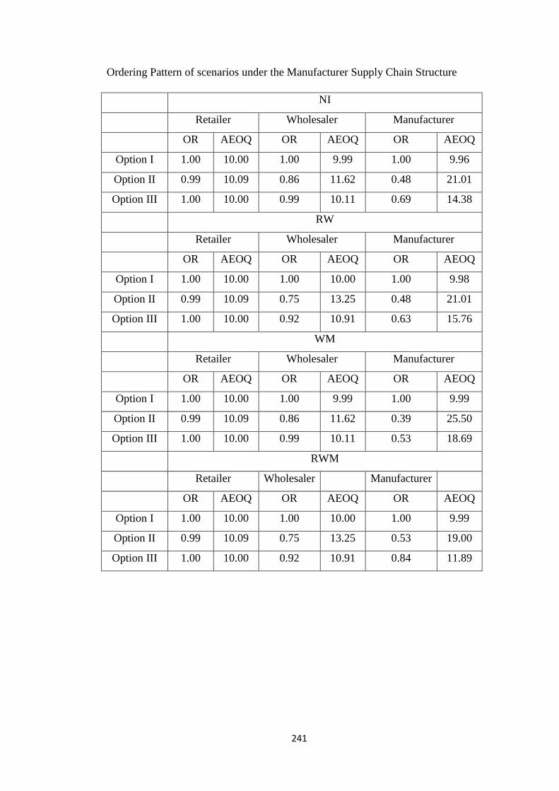
241

Ordering Pattern of scenarios under the Manufacturer Supply Chain Structure

NI



Option I 1.00 10.00 1.00 9.99 1.00 9.96

Option II 0.99 10.09 0.86 11.62 0.48 21.01

Option III 1.00 10.00 0.99 10.11 0.69 14.38

RW



Option I 1.00 10.00 1.00 10.00 1.00 9.98

Option II 0.99 10.09 0.75 13.25 0.48 21.01

Option III 1.00 10.00 0.92 10.91 0.63 15.76

WM



Option I 1.00 10.00 1.00 9.99 1.00 9.99

Option II 0.99 10.09 0.86 11.62 0.39 25.50

Option III 1.00 10.00 0.99 10.11 0.53 18.69

RWM

Retailer Wholesaler

Manufacturer


Option I 1.00 10.00 1.00 10.00 1.00 9.99

Option II 0.99 10.09 0.75 13.25 0.53 19.00

Option III 1.00 10.00 0.92 10.91 0.84 11.89

242

Ordering Pattern of scenarios under the Network Supply Chain Structure

NI



Option I 1.00 10.00 1.00 9.99 1.00 9.96

Option II 0.99 10.09 0.88 11.41 0.67 14.99

Option III 1.00 10.00 0.96 10.36 0.73 13.65

RW



Option I 1.00 10.00 1.00 10.00 1.00 9.98

Option II 0.99 10.09 0.75 13.34 0.50 20.08

Option III 1.00 10.00 0.85 11.72 0.68 14.76

WM



Option I 1.00 10.00 1.00 9.99 1.00 9.99

Option II 0.99 10.09 0.88 11.41 0.62 16.01

Option III 1.00 10.00 0.96 10.36 0.68 14.80

RWM



Option I 1.00 10.00 1.00 10.00 1.00 9.99

Option II 0.99 10.09 0.75 13.34 0.70 14.70

Option III 1.00 10.00 0.85 11.72 0.93 10.68

243

APPENDIX 4.3 BULLWHIP QUANTIFICATION OF ALL SCENARIOS

Structure Effect on Order Amplification In A Non-Breach Scenario

The variance of all orders at each tier of the supply chain in the non-breach scenario

under the various supply chain structures

Order variance at each tier

Serial WH MF NT

Op. I

Demand 4.11 4.26 4.26 4.26

R Order 4.23 4.24 4.24 4.24

W Order 4.42 4.41 4.42 4.40

M Order 4.57 4.57 4.56 4.55

Op. II

Demand 4.11 4.26 4.26 4.26

R Order 12.90 11.33 11.33 11.33

W Order 60.13 90.18 59.79 51.51

M Order 103.99 154.79 220.43 136.16

Op. III

Demand 4.11 4.26 4.26 4.26

R Order 6.17 5.88 5.88 5.88

W Order 18.20 14.78 18.19 16.09

M Order 61.20 100.85 110.05 108.98

The order amplification at the retailer, wholesaler and manufacturer computed as a

ratio to the demand variance (Chen at al. 2000a).

Order Amplification Relative to Demand variance

Serial WH MF NT

Option I Retailer 1.03 1.00 1.00 1.00

Wholesaler 1.07 1.04 1.04 1.03

Manufacturer 1.11 1.07 1.07 1.07

Option II Retailer 3.14 2.66 2.66 2.66

Wholesaler 14.63 21.19 14.05 12.10

Manufacturer 25.30 36.37 51.80 32.00

Option III Retailer 1.50 1.38 1.38 1.38

Wholesaler 4.43 3.47 4.27 3.78

Manufacturer 14.89 23.70 25.86 25.61

244


ratio to the order variance of the adjacent downstream tier, Control Theory (Jury

1974).

Order Amplification based on Control Theory

Serial WH MF NT

Option I

Retailer 1.03 1.00 1.00 1.00

Wholesaler 1.04 1.04 1.04 1.04

Manufacturer 1.03 1.03 1.03 1.03

Option II

Retailer 3.14 2.66 2.66 2.66

Wholesaler 4.66 7.96 5.28 4.55

Manufacturer 1.73 1.72 3.69 2.64

Option III

Retailer 1.50 1.38 1.38 1.38

Wholesaler 2.95 2.51 3.09 2.74

Manufacturer 3.36 6.82 6.05 6.77

Information Sharing Level Effect on Order Amplification in A Non-Breach

Scenario

The variance of all orders at each tier of the serial supply chain in the non-breach

scenario under the various supply information sharing levels.

Order variance under each ISL

NI RW WM RWM

Option I Demand 4.11 4.11 4.11 4.11

R Order 4.23 4.23 4.23 4.23

W Order 4.42 4.36 4.42 4.36

M Order 4.57 4.48 4.55 4.19

Option II Demand 4.11 4.11 4.11 4.11

R Order 12.90 12.90 12.90 12.90

W Order 60.13 100.14 60.13 100.14

M Order 103.99 104.20 153.19 80.20

Option III Demand 4.11 4.11 4.11 4.11

R Order 6.17 6.17 6.17 6.17

W Order 18.20 50.39 18.20 50.39

M Order 61.20 56.98 87.35 31.19

245


ratio to the demand variance (Chen at al. 2000a).

Order Amplification Relative to Demand variance

NI RW WM RWM

Option I

Retailer 1.03 1.03 1.03 1.03

Wholesaler 1.07 1.06 1.07 1.06

Manufacturer 1.11 1.09 1.11 1.02

Option II

Retailer 3.14 3.14 3.14 3.14

Wholesaler 14.63 24.36 14.63 24.36

Manufacturer 25.30 25.35 37.26 19.51

Option III

Retailer 1.50 1.50 1.50 1.50

Wholesaler 4.43 12.26 4.43 12.26

Manufacturer 14.89 13.86 21.25 7.59


ratio to the order variance of the adjacent downstream tier, Control Theory (Jury

1974).

Order Amplification based on Control Theory

NI RW WM RWM

Option I

Retailer 1.03 1.03 1.03 1.03

Wholesaler 1.04 1.03 1.04 1.03

Manufacturer 1.03 1.03 1.03 0.96

Option II

Retailer 3.14 3.14 3.14 3.14

Wholesaler 4.66 7.76 4.66 7.76

Manufacturer 1.73 1.04 2.55 0.80

Option III

Retailer 1.50 1.50 1.50 1.50

Wholesaler 2.95 8.17 2.95 8.17

Manufacturer 3.36 1.13 4.80 0.62

246

APPENDIX 4.4 INTERACTION EFFECT OF INFORMATION SHARING STRATEGIES AND STRUCTURAL

RECONFIGURATION STRATEGIES

Singular effect and Interaction effect of information sharing level and supply chain structure on supply chain daily operational cost

performance (‘nd’ means not statistically significant at p<0.05)


Ret.

(%)

Whole.

(%)

Manuf.

(%)

SC

Total

(%)

Ret.

(%)

Whole.

(%)

Manuf.

(%)

SC

Total

(%)

Ret.

(%)

Whole.

(%)

Manuf.

(%)

SC

Total

(%)

Singular

effect of

Structure

WH -2.1nd 0.2nd 5.3 0.2nd -3.1 8 7.1 3.4 1.3nd 11.3 4.4 5.2

MF 0.1nd 0.6nd 11 2.7nd -2.8nd -0.4nd 12.8 3.1 -1 0.3 5.9 1.9

NT -2.0nd -1.9nd 5.2 -0.4nd -3.9 4.6 12.5 3.9 1.0nd 7.5 4.5 4.1

Singular

effect of

Integration

RW 12.1 18.1 -3.1nd 10.4 5.1 4.4 -2.3nd 2.5 -1.9 -1.2nd 13 3.9

WM -2 -3.2 13.3 1.1nd -1.5 -0.8 7.5 1.7 -6.7 -6.9 24.7 5.1

RWM 20.2 30.1 10.9 20.9 4.8 5.8 11.4 7.3 -3 -2 23.8 7.4

RW and

structure

synergy

WH 12.1 23 -0.6nd 12.3 5.2 9.6 -5.5 2.9 -1.7nd 4.9 13.8 5.9

MF 12.1 18.9 5.2nd 12.5 3.8nd 4.5 8.7 5.6 -2.8nd -1.0nd 24.6 8

NT 5.5 5.9 -0.7nd 4.2 -6.4 -15 8.2 -3.9 -7.9 -10.2 19 1.7nd

WM and

structure

synergy

WH -2.9 -1.1nd 17.5 2.2nd -3.4 8.2 10.6 4.5 -3.6 5.9 28.3 11

MF -2.7nd -3.9nd 23.2 2.8nd -6.1 -3.3 13.8 1.3nd -9.5 -8.4 27.6 4.8

NT -3.7 -4.7nd 18.7 1.1nd -4.9 3.8 13 3.5 -6 -0.3nd 27.2 8.1

RWM and

structure

synergy

WH 21.4 37.6 10.5 23.5 5.1 12.3 10.8 9 -2.3nd 5.1 24.2 9.7

MF 20 30.3 22.2 23.4 3.1nd 5.6 19.7 9.3 -3.4 -1.6 31.5 10.3

NT 13.1 16.5 14.6 14.4 -8.2 -16.5 17.6 -1.9 -8.8 -11 26.6 4

247

Nature of Interaction Effect

RW WM RWM

WH MF N WH MF N WH MF N

Option

I

Retailer CA+ CO CA+ W CA- W CA+ CO CA+

Wholesaler CO CO CA+ CA- CA- W CO CO CA+

Manufacturer CA- CA+ CA- CO CO CO CO CO CO

SC Total CO CO CA+ CO CO CA+ CO CO CA+

Option

II

Retailer CA+ CA+ CA- W W W CA+ CA+ CA-

Wholesaler CO CA+ R- CA+ W CA+ CO CA+ R-

Manufacturer CA- CA+ CA+ CO CO CO CO CO CO

SC Total CO CO R- CO CO CO CO CO R-

Option

III

Retailer CA- W CA- CA- W CA- CA- W CA-

Wholesaler CA+ CA- CA- CA+ CA- CA- CA+ CA- CA-

Manufacturer CO CO CO CO CO CO CO CO CO

SC Total CO CO CO CO CO CO CO CO CO

Positive cancellation (CA+) means the resultant effect is beneficial

produced from a positive ISL and negative Structure or a negative ISL and a

positive Structure effect. A negative cancellation (CA-) occurs when the

resultant effect is negative produced either from a positive ISL and negative

Structure effect or vice versa. A negative repelling effect (R-) occurs when

the positive effect of both ISL and Structure produces a resultant negative

effect. On the other hand a positive repelling effect (R+) occurs when the

negative effect of both ISL and Structure produces a resultant positive

effect. Worsening effect (W) is generated when the resultant effect is

negative which is produced from both negative ISL and Structure effects

and a corroborating effect (CO) is felt when the resultant effect is positive

produced from a positive ISL and a positive Structure effect.

CO, CA+, and R+ symbols are all beneficial effects but CA-, R- and W are

all detrimental effects.

248

APPENDIX 5.1 INTERACTION EFFECT OF ISL AND SUPPLY STRUCTURE UNDER INFORMATION SECURITY BREACH

Interaction effect under SFDD (‘*’ means not statistically significant at p<0.05)

option I option II option III

R. Cost

%

W.

Cost %

M.

Cost %

SC

Total

%

R. Cost

%

W.

Cost %

M.

Cost %

SC

Total

%

R. Cost

%

W.

Cost %

M.

Cost %

SC

Total

%

Singular

effect of

Structure

WH -4 6 19 4 60 21 10 32 10 30 13 16

MF -4 2 25 4 60 13 15 32 8 18 16 14

NT -4 4 19 3 58 16 15 32 9 27 13 15

Singular

effect of

Integration

RW 0 0 8 2 22 -8 -14 2 -8 -1 10 1

WM -2 -4 12 1 -4 -5 7 0 -7 -7 22 4

RWM 4 5 4 4 21 -1 -11 4 -10 -4 18 2

RW and

structure

synergy

WH 3.1 17.2 16.2 10.7 77.1 16.2 -4.4 32.9 5.5 24.5 22.0 16.8

MF 2.8 11.8 9.3 10.3 74.6 9.3 7.8 34.1 3.6 16.7 32.0 17.9

NT -0.4 4.6* 7.8 2.5 75.1 7.8* -0.7 31.0 7.4* 17.4 3.7 8.6

WM and

structure

synergy

WH -5.1 4.6 20.0 4.8 59.1 20.0 13.3 32.9 5.7 26.0 34.5 22.0

MF -7.4 -4.0 7.5 3.0 55.6 7.5 15.5 28.8 -0.4* 9.7 33.8 15.3

NT -6.0 0.6* 14.2 4.1 56.7 14.2 15.3 31.0 3.5 20.4 34.2 19.6

RWM and

structure

synergy

WH 9.3 26.8 27.3 16.0 76.7 27.3 -13.8 32.8 3.5 22.3 28.0 17.8

MF 8.1 19.2 11.7 16.9 73.2 11.7 14.8 36.6 2.1 14.9 37.9 19.0

NT 3.0 9.0 4.2 9.7 69.4 4.2 10.9 31.7 -1.0* 8.8 32.6 14.3

Interaction effect under AOW (‘*’ means not statistically significant at p<0.05)

249


R. Cost

%

W.

Cost %

M.

Cost %

SC

Total

%

R. Cost

%

W.

Cost %

M.

Cost %

SC

Total

%

R. Cost

%

W.

Cost %

M.

Cost %

SC

Total

%

Singular

effect of

Structure

WH -10 -2 5 -5 8 9 7 8 -4 13 4 4

MF -12 -8 11 -6 8 1 13 8 -1 6 9 5

NT -10 -4 5 -5 7 6 12 9 -4 11 5 3

Singular

effect of

Integration

RW 6 2 12 6 12 -6 -2 2 4 0 13 6

WM -2 -7 0 -3 -2 -1 7 1 0 -2 16 6

RWM 8 6 -3 5 11 2 -2 4 3 1 19 9

RW and

structure

synergy

WH -1.5* 9.6 7.4 3.6 20.0 7.4 -5.5 8.0 1.4* 14.8 16.8 10.8

MF -2.2 3.5 0.5 2.8 18.2 0.5* 8.0 9.8 -0.3* 5.7 27.7 11.9

NT -4.5 1.7 -9.0 -0.1 13.7 -9.0 0.3 2.9 -2.5 2.4* 4.2 1.3

WM and

structure

synergy

WH -11.7 -5.2 9.4 -5.0 7.8 9.4 10.3 9.1 -4.6 13.1 26.8 12.0

MF -15.4 -15.1 -2.3 -8.5 5.0* -2.3 13.4 5.7 -6.1 3.7 28.8 9.7

NT -12.8 -9.8 5.2 -6.3 6.3 5.2 12.7 8.1 -5.6 9.3 27.2 10.8

RWM and

structure

synergy

WH 3.5 17.6 13.3* 7.3 19.8 13.3 4.9 13.0 1.3* 15.7 25.8 14.4

MF 2.0 9.5 3.1 7.5 16.5 3.1 13.2 11.7 -1.3* 5.9 31.5 13.0

NT -2.1 1.3* -10.6 1.4 9.3 -10.6 11.9 4.6 -3.5 0.5* 26.5 8.9

250

Interaction effect under PT (‘*’ means not statistically significant at p<0.05)


R. Cost

%

W.

Cost %

M.

Cost %

SC

Total

%

R. Cost

%

W.

Cost %

M.

Cost %

SC

Total

%

R. Cost

%

W.

Cost %

M.

Cost %

SC

Total

%

Singular

effect of

Structure

WH -5 -2 6 -2 0 9 7 5 -1 11 4 4

MF -3 -2 11 1 0 0 13 4 -3 0 6 2

NT -5 -4 6 -2 -1 6 13 5 -1 7 4 3

Singular

effect of

Integration

RW 10 15 -1 9 7 4 -3 3 -3 -2 13 3

WM -2 -3 13 1 -2 -1 8 2 -6 -6 25 6

RWM 17 25 10 18 7 6 11 8 -4 -2 24 7

RW and

structure

synergy

WH 8.2 18.7 10.8* 9.4 8.9 10.8 -5.1 4.8 -3.7 5.0 14.2 5.4

MF 8.4 14.7 5.4 9.7 7.5 5.4 8.9 7.4 -4.7 -1.1 24.8 7.4

NT 3.6* 4.7* -11.7* 0.3* -0.5* -11.7 1.0 -3.2* -3.9 -4.3 -5.4 -4.6*

WM and

structure

synergy

WH -5.3 -2.9* 9.2 0.8* -0.5* 9.2 10.9 6.0 -5.0 6.5 29.2 11.0

MF -5.6 -6.7 -2.6 0.5* -3.3* -2.6 14.0 2.6 -10.3 -7.3 28.1 5.0

NT -6.5 -7.3 4.8 -1.0* -2.1* 4.8 13.3 4.9 -7.5 0.3* 27.7 7.9

RWM and

structure

synergy

WH 17.0 32.4 13.9 19.8 8.7 13.9 10.4 10.7 -4.3 5.2 24.4 9.1

MF 15.7 25.2 6.6 19.9 6.7 6.6 19.4 10.9 -5.4 -1.7 31.7 9.6

NT 9.0 11.9 -14.3 11.1 -3.9* -14.3 17.5 0.3* -10.7 -10.8 26.8 3.5

251

Interaction effect under IBMS (‘*’ means not statistically significant at p<0.05)


R. Cost

%

W.

Cost %

M.

Cost %

SC

Total

%

R. Cost

%

W.

Cost %

M.

Cost %

SC

Total

%

R. Cost

%

W.

Cost %

M.

Cost %

SC

Total

%

Singular

effect of

Structure

WH -4 -1 6 -1 -1 9 7 4 0 11 4 4

MF -2 -1 11 1 -1 0 13 4 -2 0 6 2

NT -4 -4 5 -2 -2 5 13 5 -1 7 5 3

Singular

effect of

Integration

RW 10 15 -2 9 6 4 -2 3 -3 -2 13 3

WM -2 -3 13 1 -2 -1 8 2 -6 -6 25 6

RWM 18 26 10 19 6 6 11 8 -4 -3 24 7

RW and

structure

synergy

WH 9.2 20.0 10.3* 10.2 7.3 10.3 -5.1 4.0 -3.4 4.8 14.1 5.4

MF 9.4 16.0 5.0 10.5 5.9 5.0 8.9 6.7 -4.5 -1.3* 24.8 7.4

NT 4.6* 5.9* -12.9* 1.0* -2.4* -12.9 1.0 -4.2 -3.4 -4.2 -5.4 -4.4*

WM and

structure

synergy

WH -4.6 -2.2* 8.8 1.2* -1.7* 8.8 10.9 5.4 -4.8 6.2 28.9 10.9

MF -4.8 -5.8 -2.8 1.2* -4.5 -2.8 14.0 2.1 -10.3 -7.9 27.8 4.8

NT -5.7 -6.4 4.4 -0.4* -3.3 4.4 13.3 4.4 -7.3 0.0* 27.5 7.8

RWM and

structure

synergy

WH 18.2 34.1 13.2 20.9 7.1 13.2 10.6 10.0 -4.0 5.0 24.3 9.1

MF 17.0 26.9 6.2 21.0 5.1* 6.2 19.7 10.3 -5.2 -1.9 31.6 9.6

NT 10.2 13.3 -15.3 12.1 -5.8* -15.3 17.6 -0.7* -10.5 -11.1 26.7 3.4

252

Aggregate of interaction effect under all four information security breaches


R. Cost

%

W.

Cost %

M.

Cost %

SC

Total

%

R. Cost

%

W.

Cost %

M.

Cost %

SC

Total

%

R. Cost

%

W.

Cost %

M.

Cost %

SC

Total

%

Singular

effect of

Structure

WH -23 1 35 -3 66 48 32 50 5 65 27 29

MF -20 -9 58 1 67 14 53 48 2 26 37 22

NT -23 -8 35 -6 62 33 53 51 4 51 27 25

Singular

effect of

Integration

RW 27 32 17 26 48 -5 -21 10 -10 -5 49 14

WM -8 -17 38 0 -8 -8 29 4 -18 -20 88 22

RWM 47 62 21 45 45 14 9 24 -14 -8 84 25

RW and

structure

synergy

WH 19 65 45 34 113 45 -20 50 0 49 67 38

MF 18 46 20 33 106 20 34 58 -6 20 109 45

NT 3 17 -26 4 86 -26 1 27 -2 11 -3 1

WM and

structure

synergy

WH -27 -6 47 2 65 47 45 53 -9 52 119 56

MF -33 -32 0 -4 53 0 57 39 -27 -2 119 35

NT -31 -23 29 -4 58 29 54 48 -17 30 117 46

RWM and

structure

synergy

WH 48 111 68 64 112 68 12 66 -4 48 102 50

MF 43 81 28 65 101 28 67 69 -10 17 133 51

NT 20 36 -36 34 69 -36 58 36 -26 -13 113 30

253

APPENDIX 5.2 COMPARISON OF THE NATURE OF

INTERACTION EFFECT UNDER BREACH AND NON-BREACH

SCENARIOS

Since this section is only concerned with the analysis of the interaction

between ISL and structure, an examination of the interaction effect in

Appendix 5.1 reveals the state or categories of the types of interaction effect

which is presented in the subsequent tables in this section. The

state/categories of the types of interaction has been described in section

4.4.4 and these are cancellation effect (which can be positive or negative),

repelling effect (which can be positive or negative), worsening effect and

corroborating effect. A cancellation effect is observed when an agent is

favoured by structural reconfiguration and disfavoured by ISL or the other

way round. A positive cancellation effect is observed when the resultant

cancellation effect yields improvement in performance and a negative

cancellation effect is observed when the resultant effect worsens the

performance. The repelling effect occurs when both ISL and reconfiguration

are of the same nature either positive or negative producing the opposite

effect when combined. Therefore a positive repelling effect produces a

positive effect from the negative effects of ISL and reconfiguration while a

negative repelling effect produces a negative effect from the positive effects

of both ISL and structural reconfiguration. A worsening effect is observed

when both structural reconfiguration and ISL do not favour the supply

agent, hence the agent would have been better off in a serial supply chain

where no information is being shared. A corroborating effect is the case

when both structure and ISL favour the agent.

Interacting Effect of RW and Supply Chain Structure in a Breach

Scenario

To address the two issues stated in section 5.5, the categories of the

interaction effect between RW and supply chain structure is shown in the

table below. The categories of RW+Structure interaction effect under the

non-breach scenario is extracted from Appendix 4.4 and is included for

comparison purpose in the table below. Those of the breach scenarios are

deduced from Appendix 5.1. The table below therefore paints the picture of

254

how the effect categories changes from a non-breach state to a less

disruptive and less recurring breach scenario and how this changes when the

disruption duration and the RoC increases significantly.

Under the impact of IBMS, the state or category of the interaction between

RW and structure on supply chain total operating cost remains the same for

options II and III as under a non-breach scenario. However, under option I,

this changes for the RW+WH interaction from the desirable CO

(collaborating effect) in the non-breach context to a less desirable CA+

(positive cancellation) in the breach scenario. When the disruption duration

is intensified the state of the interaction of RW with the WH and MF

structure is similar to the non-breach scenario but that of the network

structure changes from the less desirable CA+ in the non-breach scenario to

the more desirable CO in the SFDD breach counterpart. A breach with

increased RoC such as is the case of AOW would cause a state change in the

interaction effect for all supply chain structures under option I scenario. CO,

CO, CA+ for WH, MF and N respectively changes to CA+, CA+, CA- in

the highly recurring breach state. Under option II, the result also shows that

a breach with less disruptive tendencies and less recurring nature have no

effect on the state of interaction between RW and structure. However when

the disruption duration and RoC increases significantly, the state of

interaction between RW and N changes from a less desirable R- to a more

desirable CO. Option III represents a more stable policy in this regard.

Regardless of the breach profile, the state of the interaction between RW

and Structure is not changed for option III.

When the result in Appendix 4.4 is compared to the result in Appendix 5.1,

it clear that the magnitude of RW+ structure effect is reduced under a breach

scenario (IBMS) for options I and III but that of option II is actually

increased. Hence the benefit of the interaction effect under IBMS security

breach is higher for option II but lower for options I and III.

255

Interaction effect between RW and Structure and the effect of security breach profile


Retailer Wholesaler Manufacturer SC Retailer Wholesaler Manufacturer SC Retailer Wholesaler Manufacturer SC

Non-Breach Scenario

WH CA+ CO CA- CO CA+ CO CA- CO CA- CA+ CO CO

MF CO CO CA+ CO CA+ CA+ CA+ CO W CA- CO CO

N CA+ CA+ CA- CA+ CA- R- CA+ R- CA- CA- CO CO

Less Disruptive and Less Recurring Breach (IBMS) Scenario

WH CA+ CA+ CA+ CA+ CA+ CO CA- CO W CA+ CO CO

MF CA+ CA+ CA+ CO CA+ CO CA+ CO W CA- CO CO

N CA+ CA+ CA+ CA+ CA- R- CA+ R- W CA- CO CO

High Disruptive and Less Recurring Breach (SFDD) Scenario

WH CA+ CA+ CO CO CO CA+ CA- CO CA+ CA+ CO CO

MF CA+ CA+ CO CO CO CA+ CA+ CO CA+ CA+ CO CO

N CA- CA+ CO CO CO CA+ CA+ CO CA+ CA+ CO CO

Less Disruptive but High Recurring Breach (AOW) Scenario

WH CA- CA+ CO CA+ CO CA+ CA- CO CA+ CA+ CO CO

MF CA- CA+ CO CA+ CO CA+ CA+ CO CA- CA+ CO CO

N CA- CA- CO CA- CO CA- CA+ CO CA- CA+ CO CO

256

Further examination reveals that this benefit tend to increase when the

security breach has higher disruptive tendencies or RoC for option II and for

option III, with the exception of the WH structure under option II where the

magnitude of interaction effect is negative and less than the non-breach

counterpart.

Interacting Effect of WM and Supply Chain Structure in a Breach

Scenario

The change in the state of interaction effect between WM and Structure due

to information security breach profile is shown in the table below. In a less

disruptive and less recurring security breach scenario, the state of the

interaction between WM and structure under options II and III remains

unchanged while that of option I is changed from a more desirable state to a

less desirable type for WH and N structures only. Under option I, only the

state of WM+N is changed from CA+ to CO under a more disruptive breach

while the state of WM+WH and WM+MF remains the same. In a more

recurring breach scenario, the state of all three structures under the influence

of WM changes to W which is a worsening effect. However, for option II,

breaches of type SFDD causes a change in state for all structure types from

CO in the non-breach scenario to CA+ in the SFDD breach scenario but

breaches of the type AOW do not effect any changes to the state of the

interaction between WM and all structure types discussed in this study.

Again the state of the WM+Structure interaction under option III appear to

be unperturbed by the incidence of security breach regardless of the breach

profile. The corroborating interaction effect remains unchanged despite

increasing recurring rate and disruption duration.

A comparison of the result for WM in Appendix 4.4 with the result for WM

shown in Appendix 5.1 reveals that for a breach profile similar to IBMS

profile, the magnitude of WM+Structure interaction effect is higher under

option II, while lower under option I but somewhat stable under option III.

257

Interaction effect between WM and Structure and the effect of security breach profile



Non-Breach Scenario

WH W CA- CO CO W CA+ CO CO CA- CA+ CO CO

MF CA- CA- CO CO W W CO CO W CA- CO CO

N W W CO CA+ W CA+ CO CO CA- CA- CO CO


WH W W CO CA+ W CA+ CO CO W CA+ CO CO

MF W W CO CO W CA- CO CO W CA- CO CO

N W W CO CA- W CA+ CO CO W CA- CO CO


WH W CA+ CO CO CA+ CA+ CO CA+ CA+ CA+ CO CO

MF W CA- CO CO CA+ CA+ CO CA+ CA- CA+ CO CO

N W CA+ CO CO CA+ CA+ CO CA+ CA+ CA+ CO CO


WH W W CA+ W CA+ CA+ CO CO CA- CA+ CO CO

MF W W CA+ W CA+ CA- CO CO CA- CA+ CO CO

N W W CA+ W CA+ CA+ CO CO CA- CA+ CO CO

258

Therefore WM+Structure interaction benefit is higher under a less

disruptive and less disruptive breach only for option II. The story changes

when the breach profile is of the SFDD type causing the magnitude of the

WM+Structure interaction effect to be greater under all three ordering

options (I, II and III). It therefore shows that a combination of WM and

structural reconfiguration offers greater benefit to the supply chain in highly

disruptive breach scenario than in the non-breach scenario. This study does

not try to infer that a security breach scenario is more desirable but only

demonstrates that the supply chain can with this WM+Structure

combination can rest assured that they would be protected even better in a

security breach state with SFDD type profile. A highly recurring breach

type however worsens the interaction effect under option I producing a

negative result but the performance under options II and III is improved

under this breach profile.

Interacting Effect of RWM and Supply Chain Structure in a Breach

Scenario

The result for the effect of security breach profile on the state of

RWM+Structure interaction effect is shown in the table below. Again the

state change from non-breach scenario to a less disruptive and less recurring

breach scenario is first examined and then the state change under increased

disruption duration and increased recurring rate is then examined. Under

IBMS type profile, only the combination that involves WH is affected with

a change in state from CO to CA+ in the option I scenario. However the

state in the options II and III scenarios are unaffected. With a more

disruptive breach, only the network structure combination is affected,

however only under options I (CA+ to CO) and II (R- to CO) scenarios. A

less disruptive but highly recurring breach is seen to cause a change in state

of the WH and MF combinations from CO to CA+ under option I scenario.

However this produces a change only under the N structure from R- to CO

in the option II scenario. Again the state of all combinations under option III

scenario remain unperturbed by breach profile.

259

Interaction effect between RWM and Structure and the effect of security breach profile



Non-Breach Scenario

WH CA+ CO CO CO CA+ CO CO CO CA- CA+ CO CO

MF CO CO CO CO CA+ CA+ CO CO W CA- CO CO

N CA+ CA+ CO CA+ CA- R- CO R- CA- CA- CO CO


WH CA+ CA+ CO CA+ CA+ CO CO CO W CA+ CO CO

MF CA+ CA+ CO CO CA+ CO CO CO W CA- CO CO

N CA+ CA+ CO CA+ CA- R- CO R- W CA- CO CO


WH CA+ CO CO CO CO CA+ CA- CO CA+ CA+ CO CO

MF CA+ CO CO CO CO CA+ CA+ CO CA+ CA+ CO CO

N CA+ CO CO CO CO CA+ CA+ CO CA- CA+ CO CO


WH CA+ CA+ CA+ CA+ CO CO CA+ CO CA+ CO CO CO

MF CA+ CA+ CA+ CA+ CO CO CA+ CO CA- CO CO CO

N CA- CA+ CA+ CA+ CO R- CA+ CO CA- CO CO CO

260

In summary, the state of interaction between RWM and structure is not affected by

changing breach profile for an option III supply chain but that of the option II is

changed only for the Network structure under conditions of high disruption duration

and high RoC. For option I, the change comes for the WH structure combination

only under IBMS and AOW breach profiles, for MF the change comes only under

AOW breach profile and for N the only change seen comes under SFDD breach

type.

261

APPENDIX 6.1 UNCERTAINTY RATING UNDER SUPPLY CHAIN STRUCTURE

Uncertainty rating in a Parameter based ordering system (Option I).

WH STRUCTURE


Hold Backlog R Total Hold Backlog W Total Hold Backlog M Total Average

SFDD 1 0 1 0 0 0 0 0 0 0

AOW 1 0 1 0 0 0 0 0 0 0

PT 1 0 1 0 0 0 0 1 1 0

IBMS 1 0 1 1 0 1 0 1 1 1

MF STRUCTURE



SFDD 1 0 1 1 0 1 0 0 0 0

AOW 1 0 1 0 0 0 0 0 0 0

PT 1 0 1 0 0 0 0 1 1 0

IBMS 1 1 1 1 1 1 3 1 2 1

NT STRUCTURE



SFDD 1 0 1 0 0 0 0 0 0 0

AOW 1 0 1 0 0 0 0 0 0 0

PT 1 0 1 0 0 0 0 1 1 0

IBMS 1 0 1 1 0 1 0 1 1 1

262

Uncertainty rating in a Batch ordering system (Option II).

WH



SFDD 0 3 2 0 0 0 1 0 1 1

AOW 1 0 1 1 1 1 1 1 1 1

PT 1 1 1 1 1 1 1 1 1 1

IBMS 1 1 1 1 1 1 1 1 1 1

MF



SFDD 0 3 2 0 0 0 1 1 1 1

AOW 1 0 1 1 1 1 1 1 1 1

PT 1 1 1 1 1 1 1 1 1 1

IBMS 1 1 1 1 1 1 1 1 1 1

NT



SFDD 0 3 2 0 0 0 1 0 1 1

AOW 1 0 1 1 1 1 1 1 1 1

PT 1 1 1 1 1 1 1 1 1 1

IBMS 1 1 1 1 1 1 1 1 1 1

263

Uncertainty rating in a Combined Batch-and-Parameter based ordering system (Option III).

WH


E. I. Hold Backlog R Total Hold Backlog W Total Hold Backlog M Total Average

SFDD 0 0 0 1 0 1 0 1 1 0

AOW 0 1 1 0 0 0 1 0 1 0

PT 0 1 1 0 1 1 1 1 1 1

IBMS 0 1 1 0 1 1 1 1 1 1

MF



SFDD 0 1 1 1 1 1 3 1 2 1

AOW 0 0 0 0 0 0 0 0 0 0

PT 0 1 1 0 0 0 1 1 1 1

IBMS 0 1 1 0 1 1 1 1 1 1

NT



SFDD 0 0 0 1 0 1 0 1 1 0

AOW 0 1 1 0 0 0 1 0 1 0

PT 0 1 1 0 1 1 0 1 1 1

IBMS 0 1 1 1 1 1 1 1 1 1

264

APPENDIX 6.2 UNCERTAINTY RATING UNDER INFORMATION INTEGRATION

Uncertainty rating in a Parameter based ordering system (Option I).

RW



SFDD 1 1 1 0 0 0 0 1 1 1

AOW 1 0 1 0 1 1 1 0 1 1

PT 1 0 1 0 1 1 0 0 0 0

IBMS 1 0 1 1 1 1 0 0 0 1

WM



SFDD 1 0 1 1 1 1 0 0 0 1

AOW 1 0 1 0 0 0 0 0 0 0

PT 1 0 1 0 0 0 0 1 1 0

IBMS 1 0 1 0 0 0 1 1 1 1

RWM



SFDD 1 1 1 0 1 1 1 0 1 1

AOW 1 0 1 1 0 1 1 0 1 1

PT 1 0 1 0 1 1 0 1 1 1

IBMS 1 0 1 1 1 1 0 1 1 1

265

Uncertainty rating in a Batch ordering system (Option II).

RW



SFDD 1 3 2 3 0 2 3 2 3 2

AOW 1 2 2 1 0 1 3 1 2 1

PT 0 1 1 1 1 1 3 1 2 1

IBMS 1 1 1 1 1 1 2 1 2 1

WM



SFDD 1 3 2 1 1 1 1 0 1 1

AOW 1 1 1 1 1 1 1 1 1 1

PT 1 1 1 1 1 1 1 1 1 1

IBMS 1 1 1 1 1 1 1 1 1 1

RWM



SFDD 1 3 2 3 1 2 1 1 1 2

AOW 1 2 2 2 0 1 0 1 1 1

PT 0 1 1 0 1 1 0 0 0 0

IBMS 1 1 1 1 1 1 0 0 0 1

266

Uncertainty rating in a Combined Batch-and-Parameter based ordering system (Option III).

RW



SFDD 1 0 1 0 1 1 1 0 1 1

AOW 0 0 0 0 0 0 1 0 1 0

PT 0 0 0 0 1 1 0 1 1 0

IBMS 0 1 1 1 1 1 1 1 1 1

WM



SFDD 1 1 1 1 0 1 1 0 1 1

AOW 1 0 1 1 0 1 1 0 1 1

PT 0 0 0 0 0 0 1 1 1 0

IBMS 0 0 0 0 1 1 1 1 1 1

RWM



SFDD 1 0 1 0 1 1 1 0 1 1

AOW 0 0 0 1 1 1 0 1 1 1

PT 0 0 0 0 1 1 1 1 1 1

IBMS 0 1 1 1 1 1 1 1 1 1

267

APPENDIX 6.3 UNCERTAINTY RATING UNDER INFORMATION INTEGRATION AND SUPPLY STRUCTURE INTERACTION

Uncertainty rating under WH structure and information integration interaction in a Parameter based ordering system (Option I).

4



SFDD 0 1 1 0 1 1 0 1 1 1

AOW 0 0 0 0 0 0 0 0 0 0

PT 1 0 1 1 1 1 0 0 0 1

IBMS 1 0 1 1 1 1 1 0 1 1

WM+WH



SFDD 1 0 1 0 0 0 1 0 1 0

AOW 1 0 1 0 0 0 1 1 1 1

PT 1 0 1 0 0 0 0 1 1 0

IBMS 1 0 1 1 0 1 1 0 1 1

RWM+WH



SFDD 0 1 1 0 0 0 1 0 1 0

AOW 0 0 0 0 0 0 1 1 1 0

PT 1 0 1 1 1 1 0 1 1 1

IBMS 1 1 1 1 1 1 1 1 1 1

268

Uncertainty rating under MF structure and information integration interaction in a Parameter based ordering system (Option I).

RW+MF



SFDD 0 1 1 0 0 0 0 1 1 0

AOW 0 0 0 0 0 0 0 0 0 0

PT 1 0 1 0 1 1 0 0 0 0

IBMS 1 1 1 1 1 1 1 1 1 1

WM+MF



SFDD 1 1 1 1 1 1 0 0 0 1

AOW 1 0 1 1 1 1 0 0 0 1

PT 1 1 1 1 1 1 1 1 1 1

IBMS 1 1 1 1 1 1 1 1 1 1

RWM+MF



SFDD 0 0 0 0 0 0 1 0 1 0

AOW 0 0 0 0 0 0 0 0 0 0

PT 1 0 1 0 1 1 1 1 1 1

IBMS 1 0 1 1 1 1 1 1 1 1

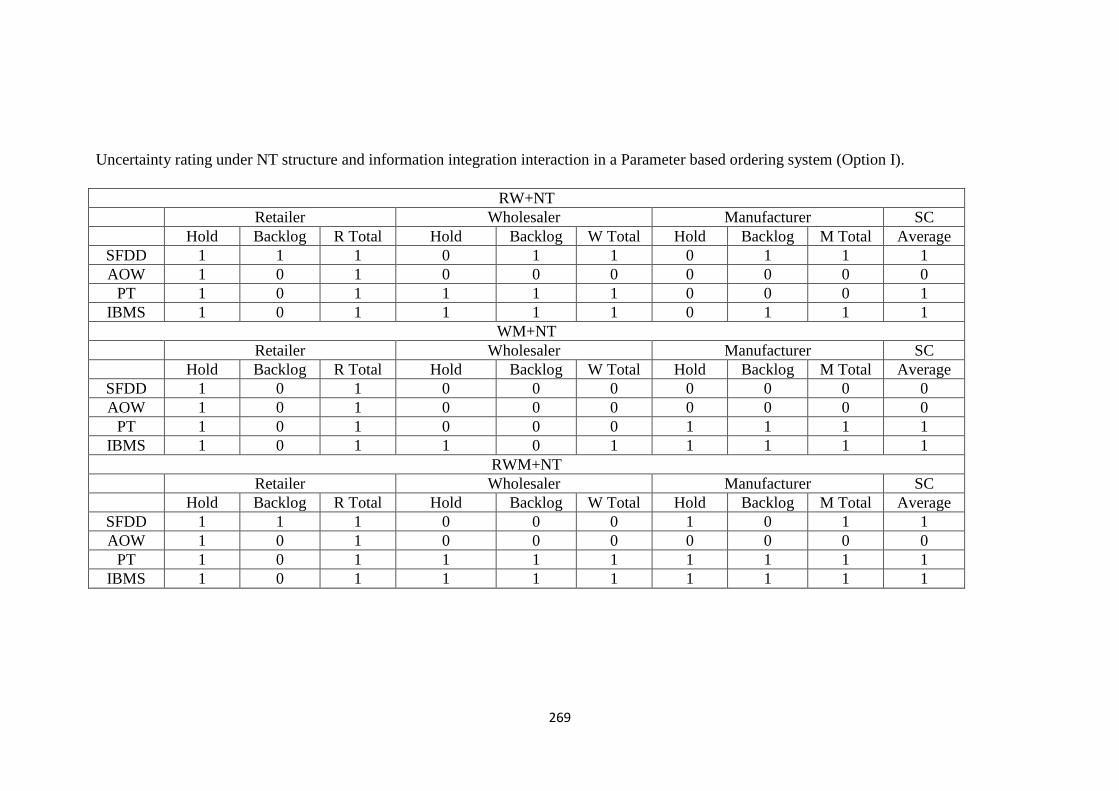
269

Uncertainty rating under NT structure and information integration interaction in a Parameter based ordering system (Option I).

RW+NT



SFDD 1 1 1 0 1 1 0 1 1 1

AOW 1 0 1 0 0 0 0 0 0 0

PT 1 0 1 1 1 1 0 0 0 1

IBMS 1 0 1 1 1 1 0 1 1 1

WM+NT



SFDD 1 0 1 0 0 0 0 0 0 0

AOW 1 0 1 0 0 0 0 0 0 0

PT 1 0 1 0 0 0 1 1 1 1

IBMS 1 0 1 1 0 1 1 1 1 1

RWM+NT



SFDD 1 1 1 0 0 0 1 0 1 1

AOW 1 0 1 0 0 0 0 0 0 0

PT 1 0 1 1 1 1 1 1 1 1

IBMS 1 0 1 1 1 1 1 1 1 1

270

Uncertainty rating under WH structure and information integration interaction in a Batch ordering system (Option II).

RW+WH



SFDD 0 3 2 3 0 2 1 0 1 1

AOW 0 1 1 1 0 1 1 1 1 1

PT 1 1 1 1 0 1 1 1 1 1

IBMS 1 1 1 1 1 1 1 1 1 1

WM+WH



SFDD 0 3 2 0 0 0 1 0 1 1

AOW 1 0 1 1 1 1 1 1 1 1

PT 1 1 1 1 1 1 1 1 1 1

IBMS 1 1 1 1 1 1 1 1 1 1

RWM+WH



SFDD 0 3 2 2 0 1 1 1 1 1

AOW 0 1 1 1 0 1 0 0 0 0

PT 1 1 1 1 0 1 1 1 1 1

IBMS 1 1 1 1 1 1 1 1 1 1

271

Uncertainty rating under MF structure and information integration interaction in a Batch ordering system (Option II).

RW+MF



SFDD 0 3 2 3 0 2 1 0 1 1

AOW 1 1 1 1 0 1 1 1 1 1

PT 1 1 1 0 1 1 1 1 1 1

IBMS 1 1 1 1 1 1 1 1 1 1

WM+MF



SFDD 0 3 2 0 0 0 1 1 1 1

AOW 1 1 1 1 1 1 1 1 1 1

PT 1 1 1 1 1 1 1 1 1 1

IBMS 1 1 1 1 1 1 1 1 1 1

RWM+MF



SFDD 0 3 2 3 0 2 0 0 0 1

AOW 1 1 1 1 0 1 0 0 0 1

PT 1 1 1 0 1 1 0 0 0 1

IBMS 1 1 1 1 1 1 1 1 1 1

272

Uncertainty rating under NT structure and information integration interaction in a Batch ordering system (Option II).

RW+NT



SFDD 0 3 2 3 0 2 3 1 2 2

AOW 1 1 1 1 0 1 3 1 2 1

PT 1 1 1 1 1 1 2 1 2 1

IBMS 1 1 1 1 1 1 2 1 2 1

WM+NT



SFDD 0 3 2 0 0 0 1 0 1 1

AOW 1 0 1 1 1 1 1 1 1 1

PT 1 1 1 1 1 1 1 1 1 1

IBMS 1 1 1 1 1 1 1 1 1 1

RWM+NT



SFDD 0 2 1 2 0 1 0 0 0 1

AOW 0 1 1 0 0 0 0 0 0 0

PT 1 1 1 1 1 1 1 1 1 1

IBMS 1 1 1 1 1 1 1 1 1 1

273

Uncertainty rating under WH structure and information integration interaction in a Combined Batch-and-Parameter based ordering system

(Option III).

RW+WH



SFDD 0 0 0 0 0 0 0 0 0 0

AOW 0 0 0 0 1 1 1 0 1 0

PT 0 0 0 1 1 1 1 1 1 1

IBMS 1 1 1 1 1 1 2 1 2 1

WM+WH



SFDD 0 1 1 1 0 1 1 1 1 1

AOW 0 0 0 0 1 1 0 1 1 0

PT 0 1 1 0 1 1 0 0 0 0

IBMS 0 1 1 0 1 1 1 0 1 1

RWM+WH



SFDD 0 0 0 0 0 0 1 0 1 0

AOW 0 0 0 0 1 1 1 0 1 0

PT 0 0 0 1 1 1 0 1 1 1

IBMS 0 0 0 1 1 1 1 1 1 1

274

Uncertainty rating under MF structure and information integration interaction in a Combined Batch-and-Parameter based ordering system

(Option III).

RW+MF



SFDD 0 0 0 0 0 0 0 0 0 0

AOW 0 0 0 0 1 1 1 1 1 1

PT 0 0 0 0 1 1 1 1 1 1

IBMS 1 1 1 1 1 1 1 1 1 1

WM+MF



SFDD 0 1 1 1 1 1 0 0 0 1

AOW 0 0 0 1 1 1 0 1 1 1

PT 0 1 1 1 1 1 1 1 1 1

IBMS 1 1 1 1 1 1 1 1 1 1

RWM+MF



SFDD 0 0 0 0 0 0 0 0 0 0

AOW 0 0 0 0 0 0 1 0 1 0

PT 0 0 0 1 1 1 1 1 1 1

IBMS 0 1 1 1 1 1 1 1 1 1

275

Uncertainty rating under NT structure and information integration interaction in a Combined Batch-and-Parameter based ordering system

(Option III).

RW+NT



SFDD 0 0 0 0 0 0 0 0 0 0

AOW 0 0 0 0 1 1 0 0 0 0

PT 0 1 1 1 1 1 1 1 1 1

IBMS 0 1 1 1 1 1 1 1 1 1

WM+NT



SFDD 0 1 1 1 0 1 0 0 0 0

AOW 0 0 0 0 1 1 1 0 1 0

PT 0 1 1 0 1 1 0 1 1 1

IBMS 0 1 1 0 1 1 1 1 1 1

RWM+NT



SFDD 0 0 0 0 0 0 1 0 1 0

AOW 0 0 0 0 1 1 0 0 0 0

PT 0 1 1 1 1 1 1 1 1 1

IBMS 0 1 1 1 1 1 1 1 1 1

276

REFERENCE LIST

Agrawal, S., Sengupta, R. N. & Shanker, K. (2009), Impact of information sharing

and lead time on bullwhip effect and on-hand inventory. European Journal of

Operational Research, 192, 576-593.

Airmic, Alarm & Irm 2010. A structured approach to enterprise risk management.

Airoldi, E. M., Bai, X. & Malin, B. A. (2011), An entropy approach to disclosure

risk assessment: Lessons from real applications and simulated domains.

Decision Support Systems, 51, 10-20.

Altay, N. & Ramirez, A. (2010), Impact of disasters on firms in different sectors:

Implications for supply chains. Journal of Supply Chain Management, 46,

59-80.

Amir, M. S. (2009), It's written in the cloud: The hype and promise of cloud

computing. Journal of Enterprise Information Management, 23, 131-134.

Armbrust, M., Fox, A., Griffith, R., Joseph, A., Katz, R., Konwinski, A., Lee, G.,

Patterson, D., Rabkin, A., Stoica, I., and Zaharia, M., (2010), A view of

cloud computing. Communications of the ACM, 53 (4), 50-58.

Arrow, K. J., Harris, T. & Marschak, J. (1951), Optimal inventory policy.

Econometrica, 19, 250-272.

Axsäter, S. (1996), Using the deterministic eoq formula in stochastic inventory

control. Management Science, 42, 830-834.

Axsäter, S. 2003. Supply chain operations: Serial and distribution inventory systems.

In: GRAVES, S. C. & KOK, A. G. D. (eds.) Handbooks in operations

research and management science. Elsevier.

Axsäter, S. & Juntti, L. (1997), Comparison of echelon stock and installation stock

policies with policy adjusted order quantities. International Journal of

Production Economics, 48, 1-6.

Baganha, M. P. & Cohen, M. A. (1998), The stabilizing effect of inventory in supply

chains. Oper. Res., 46, 72-83.

Baker, W., Goudie, M., Hutton, A., Hylender, C. D., Niemantsverdriet, J., Novak,

C., Ostertag, D., Porter, C., Rosen, M., Sartin, B. & Tippett, P. 2010. 2010

data breach investigations report. Verizon RISK Team in cooperation with the

United States Secret Service.

Banerjee, A., Burton, J. & Banerjee, S. (1996), Heuristic production triggering

mechanisms under discrete unequal inventory withdrawals. International

Journal of Production Economics, 45, 83-90.

Beamon, B. M. & Chen, V. C. P. (2001), Performance analysis of conjoined supply

chains. International Journal of Production Research, 39, 3195-3218.

Belal, C., Morshed, U. C. & Clare, D. (2008), Challenges relating to rfid

implementation within the electronic supply chain management - a practical

approach. Studies in Computational Intelligence, 149.

Bellefeuille, C. L. 2005. Quantifying and managing the risk of information security

breaches to the supply chain. Master of Engineering in Logistics,

Massachusetts Institute of Technology.

Bensoussan, A., Cakanyildirim, M. & Sethi, S. (2007), Optimal ordering policies for

inventory problems with dynamic information delays. Production and

Operations Management, 16, 241-256.

Bezzi, M. (2007), An entropy based method for measuring anonymity. In: Third

International Conference on Security and Privacy in Communications

Networks and the Workshops 17-21 Sept. 2007. IEEE, 28-32.

277

Bourland, K. E., Powell, S. G. & Pyke, D. F. (1996), Exploiting timely demand

information to reduce inventories. European Journal of Operational

Research, 92, 239-253.

Bozarth, C. C., Warsing, D. P., Flynn, B. B. & Flynn, E. J. (2009), The impact of

supply chain complexity on manufacturing plant performance. Journal of

Operations Management, 27, 78-93.

Brightman, J. (2011), Playstation network crisis may cost sony billions. Industry

Gamers [Online]. Available:

http://www.industrygamers.com/news/playstation-network-crisis-may-cost-

sony-billions/ [Accessed 21-09-2011].

Buttell, A. E. (2010), 6 reasons to switch to cloud computing. Journal of Financial

Planning, 6-7.

Capraro, A. J., Broniarczyk, S. & Srivastava, R. K. (2003), Factors influencing the

likelihood of customer defection: The role of consumer knowledge. Journal

of the Academy of Marketing Science, 31, 164-175.

Carter, T. 2011. Lecture notes on information theory and entropy. Complex Systems

Summer School, Santa Fe.

Chan, F. T. S. & Zhang, T. (2011), The impact of collaborative transportation

management on supply chain performance: A simulation approach. Expert

Systems with Applications, 38, 2319-2329.

Chan, H. K. & Chan, F. T. S. (2009), Effect of information sharing in supply chains

with flexibility. International Journal of Production Research, 47, 213-232.

Chatfield, D. C., Kim, J. G., Harrison, T. P. & Hayya, J. C. (2004), The bullwhip

effect—impact of stochastic lead time, information quality, and information

sharing: A simulation study. Production and Operations Management, 13,

340-353.

Chen, F. (1998), Echelon reorder points, installation reorder points, and the value of

centralized demand information. Manage. Sci., 44, 221-234.

Chen, F., Drezner, Z., Ryan, J. K. & Simchi-Levi, D. (2000), Quantifying the

bullwhip effect in a simple supply chain: The impact of forecasting, lead

times, and information. Management Science, 46, 436–443.

Chen, F. & Samroengraja, R. (2004), Order volatility and supply chain costs. Oper.

Res., 52, 707-722.

Chen, Y. F. & Disney, S. M. (2003), The order-up-to policy “sweet spot” - using

proportional controllers to eliminate the bullwhip problem In: EUROMA

POMS Conference, Como Lake, Italy.

Cheng, J.-H. (2010), Inter-organizational relationships and information sharing in

supply chains. International Journal of Information Management, In Press,

Corrected Proof.

Childerhouse, P. & Towill, D. R. (2003), Simplified material flow holds the key to

supply chain integration. Omega, 31, 17-27.

Cimino, A., Longo, F. & Mirabelli, G. (2010), A general simulation framework for

supply chain modeling: State of the art and case study. INTERNATIONAL

JOURNAL OF COMPUTER SCIENCE ISSUES, 7, 1-9.

Colotla, I., Shi, Y. & J., M. (2003), Operation and performance of international

manufacturing networks. International Journal of Operations & Production

Management, 23, 1181-1206.

http://www.industrygamers.com/news/playstation-network-crisis-may-cost-sony-billions/

http://www.industrygamers.com/news/playstation-network-crisis-may-cost-sony-billions/

278

Craighead, C. W., Blackhurst, J., Rungtusanatham, M. J. & Handfield, R. B. (2007),

The severity of supply chain disruptions: Design characteristics and

mitigation capabilities. Decision Sciences, 38, 131-156.

Cusumano, M. (2010), Technology strategy and management: Cloud computing and

saas as new computing platforms. Communications of the ACM, 53, 27-29.

Deane, J., Ragsdale, C., Rakes, T. & Rees, L. (2009), Managing supply chain risk

and disruption from it security incidents. Operations Management Research,

2, 4-12.

Dekkers, R. & Bennett, D. (2009), Industrial networks of the future: Review of

research and practice. 978-1-84882-468-3.

Deng, Y., Pang, J. & Wu, P. (2007), Measuring anonymity with relative entropy. In:

Dimitrakos, T., Martinelli, F., Ryan, P. & Schneider, S. (eds.) Formal aspects

in security and trust. Springer Berlin / Heidelberg.

Devaraj, S., Krajewski, L. & Wei, J. C. (2007), Impact of ebusiness technologies on

operational performance: The role of production information integration in

the supply chain. Journal of Operations Management, 25, 1199-1216.

Disney, S. M. & Lambrecht, M. R. (2007), On replenishment, forecasting, and the

bullwhip effect in supply chains. Foundation and Trends in Technology,

Information and Operations Management, 2, 1-80.

Durkee, D. (2010), Why cloud computing will never be free. Communications of the

ACM, 53, 62-69.

Ernst&Young 2011. Cloud computing issues and impacts. Global Technology

Industry Discussion Series.

Frizelle, G. & Efstathiou, J. (2002), Seminar notes on 'measuring complex systems'.

London School of Economics.

Frizelle, G. & Woodcock, E. (1995), Measuring complexity as an aid to developing

operational strategy. International Journal of Operations & Production

Management, 15, 26-39.

Gerber, M. & Von Solms, R. (2005), Management of risk in the information age.

Computers & Security, 24, 16-30.

Goel, S. & Shawky, H. A. (2009), Estimating the market impact of security breach

announcements on firm values. Information & Management, 46, 404-410.

Gordon, L. A., Loeb, M. P. & Lucyshyn, W. (2003), Sharing information on

computer systems security: An economic analysis. Journal of Accounting

and Public Policy, 22, 461-485.

Gunasekaran, A. & Ngai, E. W. T. (2004), Information systems in supply chain

integration and management. European Journal of Operational Research,

159, 269-295.

Hart, C., Doherty, N. & Ellis-Chadwick, F. (2000), Retailer adoption of the internet

implications for retail marketing. European Journal of Marketing, 34, 954-

974.

Hennig-Thurau, T. & Klee, A. (1997), The impact of customer satisfaction and

relationship quality on customer retention: A critical reassessment and model

development. Psychology and Marketing, 14, 737-764.

Hoffman, J. L. & Lowitt, E. M. (2008), Reducing the risk of customer defection.

Institute for High Performance Business. Accenture Research Note

Hoole, R. (2005), Five ways to simplify your supply chain. Supply Chain

Management: An International Journal, 10, 3-6.

279

Hosoda, T. & Disney, S. M. (2004), The role of an ordering policy as an inventory

and cost controller. Logistics Research Network Annual Conference. Dublin,

Ireland.

Hosoda, T. & Disney, S. M. (2006), On variance amplification in a three-echelon

supply chain with minimum mean square error forecasting. Omega, 34, 344-

358.

Humphreys, P. K., Lai, M. K. & Sculli, D. (2001), An inter-organizational

information system for supply chain management. International Journal of

Production Economics, 70, 245-255.

Ingalls, R. G. (2008), Introduction to simulation. In: S. J. MASON, R. R. H., L.

MÖNCH, O. ROSE, T. JEFFERSON, J. W. FOWLER, ed. Proceedings of

the 2008 Winter Simulation Conference, Miami, FL, USA. IEEE, 17-26.

Jammernegg, W. & Reiner, G. (2007), Performance improvement of supply chain

processes by coordinated inventory and capacity management. International


Kaplan, S. & Garrick, J. B. (1981), On quantitative definition of risk. Risk Analysis,

1, 11-27.

Kappelman, L. A. & Richards, T. C. (1995), Conducting business on the information

superhighway: A manager's guide to electronic data. Business Forum, 20, 29.

Kelton, D. W., Sadowski, R. P. & Swets, N. B. (2010), Simulation with arena,

Singapore, McCraw Hill.

Kim, W., Jeong, O.-R., Kim, C. & So, J. (2011), The dark side of the internet:

Attacks, costs and responses. Information Systems, 36, 675-705.

Kleijnen, J. P. C. (1995), Verification and validation of simulation models. European

Journal of Operational Research, 82, 145-162.

Kristal, M. M., Huang, X. & Roth, A. V. (2010), The effect of an ambidextrous

supply chain strategy on combinative competitive capabilities and business

performance. Journal of Operations Management, 28, 415-429.

Kulp, S. C., Lee, H. L. & Ofek, E. (2004), Manufacturer benefits from information

integration with retail customers. Management Science, 50, 431-444.

Lancioni, R. A., Smith, M. F. & Schau, H. J. (2003), Strategic internet application

trends in supply chain management. Industrial Marketing Management, 32,

211-217.

Lau, J. S. K., Huang, G. Q. & L., M. K. (2002), Web-based simulation portal for

investigating impacts of sharing production information on supply chain

dynamics from the perspective of inventory allocation. Integrated

Manufacturing Systems, 13, 345-358.

Lau, J. S. K., Huang, G. Q. & Mak, K. L. (2004), Impact of information sharing on

inventory replenishment in divergent supply chains. International Journal of

Production Research, 42, 919-941.

Lau, R. S. M., Xie, J. & Zhao, X. (2008), Effects of inventory policy on supply chain

performance: A simulation study of critical decision parameters. Computers

& Industrial Engineering, 55, 620-633.

Law, A. M. (2007), Simulation modelling and analysis, New York, McGraw-Hill

companies.

Lee, H. L., Padmanabhan, V. & Whang, S. (1997), The bullwhip effect in supply

chains. Sloan Management Review, 38, 93-102.

Lee, H. L., Padmanabhan, V. & Whang, S. (2004), Information distortion in a supply

chain: The bullwhip effect. Management Science, 50, 1875-1886.

280

Li, J., Sikora, R., Shaw, M. J. & Woo Tan, G. (2006), A strategic analysis of inter

organizational information sharing. Decision Support Systems, 42, 251-266.

Li, S. & Lin, B. (2006), Accessing information sharing and information quality in

supply chain management. Decision Support Systems, 42, 1641-1656.

Loch, K. D., Carr, H. H. & Warkentin, M. E. (1992), Threats to information systems:

Today's reality, yesterday's understanding. MIS Quarterly: Management

Information Systems, 16, 173-186.

Marston, S., Li, Z., Bandyopadhyay, S., Zhang, J. & Ghalsasi, A. (2011), Cloud

computing -- the business perspective. Decision Support Systems, 51, 176-

189.

Martínez-Olvera, C. (2008), Entropy as an assessment tool of supply chain

information sharing. European Journal of Operational Research, 185, 405-

417.

Mills, J. (2004), A strategic review of supply networks. International Journal of

Operations & Production Management, 24, 1012-1036Intern.

Mitra, S. & Chatterjee, A. K. (2004), Echelon stock based continuous review (r,q)

policy for fast moving items. Omega, 32, 161-166.

Mitroff, I. I. & Alpaslan, M. C. (2003), Preparing for evil. Harvard Business Review,

81, 109-115.

Mukhopadhyay, T. & Kekre, S. (2002), Strategic and operational benefits of

electronic integration in b2b procurement processes. Management Science,

48, 1301-1313.

Munoz, A. & Clements, M. D. (2008), Disruptions in information flow: A revenue

costing supply chain dilemma. J. Theor. Appl. Electron. Commer. Res., 3, 30-

40.

Newman, J. (2011), Experts on psn hack: Sony could have done more. Security

[Online]. Available:

http://www.pcworld.com/article/227770/experts_on_psn_hack_sony_could_

have_done_more.html [Accessed 21-09-2011].

Olson, D. L. & Wu, D. D. (2010), A review of enterprise risk management in supply

chain. Kybernetes, 39, 694-706.

Osawa, J. (2011), As sony counts hacking costs, analysts see billion-dollar repair

bill. Total Telecom Plus [Online]. Available:

http://www.totaltele.com/view.aspx?ID=464556.

Ouyang, A. (2012a), Information security & risk management domain. CISSP®

Common Body of Knowledge Review. California: Creative Commons.

Ouyang, A. (2012b), Operations security domain. CISSP Common Body of

Knowledge Review. Creative Commons.

Papanagnou, C. & Halikias, G. D. (2006), Analysing different ordering policies in a

series supply chain by using coloured petri nets. In: European Conference on

Modelling and Simulation (ECMS), Bonn, Germany.

Phillips, T. 2011. Playstation network hack 'could cost sony $1.5billion' Metro.

Pidd, M. (2003), Tools for thinking: Modelling in management science, Chichester,

John Wiley and Sons Ltd.

Pisello, T. (2004), Is there a business case for it security? Security Management

[Online]. [Accessed 22nd April 2011].

Plenert, G. J. 2002. International operations management. Copenhagen, DNK:

Copenhagen Business School Press.

http://www.pcworld.com/article/227770/experts_on_psn_hack_sony_could_have_done_more.html

http://www.pcworld.com/article/227770/experts_on_psn_hack_sony_could_have_done_more.html

http://www.totaltele.com/view.aspx?ID=464556

281

Pollack, D. (2011), Sony breach now a class action. idexperts Blog [Online].

Available: http://www2.idexpertscorp.com/blog/single/sony-breach-now-a-

class-action/ [Accessed 21-09-2011].

Potter, C. & Beard, A. 2012. Information security breach survey 2012. Information

Security Breach Survey

Rainer, R. K., Snyder, C. A. & Carr, H. H. (1991), Risk analysis for information

technology. Journal of Management Information Systems, 8, 129-147.

Randall, T. & Ulrich, K. (2001), Product variety, supply chain structure, and firm

performance: Analysis of the u.S. Bicycle industry. Management Science, 47,

1588-1604.

Rao, S. & Goldsby, T. J. (2009), Supply chain risks: A review and typology.

International Journal of Logistics Management, 20, 97-123.

Raschke, R. L. (2010), Process-based view of agility: The value contribution of it

and the effects on process outcomes. International Journal of Accounting

Information Systems, 11(4), 297-313.

Rees, L. P., Deane, J. K., Rakes, T. R. & Baker, W. H. (2011), Decision support for

cybersecurity risk planning. Decision Support Systems, 51(3), 493-505.

Richardson, R. (2009). 14th annual csi computer crime and security survey. In:

PETERS, S. (ed.) CSI Computer Crime and Security Survey. Computer

Security Institute.

Robinson, S. (2004), The practice of model development and use, Chichester,

England, John Wiley and Sons Ltd.

Ronen, B. & Karp, R. (1994), An information entropy approach to the small-lot

concept. Engineering Management, IEEE Transactions on, 41, 89-92.

Samir, D. (2008), Predicting and managing supply chain risks. International Series

in Operations Research & Management Science, 124.

Samy, G. N., Ahmad, R. & Ismail, Z. (2010), Security threats categories in

healthcare information systems. Health Informatics Journal, 16, 201.

Sargent, R. G. (2010), Verification and validation of simulation models. In:

Simulation Conference (WSC), Proceedings of the 2010 Winter, 5-8 Dec.

2010. 166-183.

Schmitt, A. J. & Singh, M. (2009), Quantifying supply chain disruption risk using

monte carlo and discrete-event simulation. In: M. D. ROSSETTI, R. R. H.,

B. JOHANSSON, A. DUNKIN, AND R. G. INGALLS, ed. Proceedings of

the 2009 Winter Simulation Conference, Austin, Texas. IEEE.

Schwartz, J. D., Wang, W. & Rivera, D. E. (2006), Simulation-based optimization of

process control policies for inventory management in supply chains.

Automatica, 42, 1311-1320.

Serdarasan, S. (2013), A review of supply chain complexity drivers. Computers &

Industrial Engineering, 66, 533-540.

Shannon, C. E. (1948), A mathematical theory of communication. The Bell System

Technical Journal, 27, 379-423, 623-656.

Shannon, R. E. 1998. Introduction to the art and science of simulation. Proceedings

of the 30th conference on Winter simulation. Washington, D.C., United

States: IEEE Computer Society Press.

Shuiabi, E., Thomson, V. & Bhuiyan, N. (2005), Entropy as a measure of operational

flexibility. European Journal of Operational Research, 165, 696-707.

Sivadasan, S., Efstathiou, J., Frizelle, G., Shirazi, R. & Calinescu, A. (2002), An

information-theoretic methodology for measuring the operational complexity

http://www2.idexpertscorp.com/blog/single/sony-breach-now-a-class-action/

http://www2.idexpertscorp.com/blog/single/sony-breach-now-a-class-action/

282

of supplier-customer systems. International Journal of Operations &

Production Management, 22, 80-102Interna.

Smith, R. (2009), Computing in the cloud. Research Technology Management, 52,

/Oct2009,-68.

Southard, P. B. & Swenseth, S. R. (2008), Evaluating vendor-managed inventory

(VMI) in non-traditional environments using simulation. International


Sterman, J. D. (1989), Modeling managerial behavior: Misperceptions of feedback in

a dynamic decision making experiment. Management Science, 35, 321-339.

Stock, G. N., Greis, N. P. & Kasarda, J. D. (2000), Enterprise logistics and supply

chain structure: The role of fit. Journal of Operations Management, 18, 531-

547.

Stoneburner, G., Goguen, A. & Feringa, A. 2002. Risk management guide for

information technology systems. Recommendations of the National Institute

of Standards and Technology. Gaithersburg, MD: National Institute of

Standards and Technology.

Subashini, S. & Kavitha, V. (2011), A survey on security issues in service delivery

models of cloud computing. Journal of Network and Computer Applications,

34, 1-11.

Swaminathan, J. M., Smith, S. F. & Sadeh, N. M. (1998), Modeling supply chain

dynamics: A multiagent approach. Decision Sciences, 29, 607-632.

Tee, Y.-S. & Rossetti, M. D. (2002), A robustness study of a multi-echelon

inventory model via simulation. International Journal of Production

Economics, 80, 265-277.

Vasconcelos, B. C. & Marques, M. P. (2000), Reorder quantities for (Q,R) inventory

models. The Journal of the Operational Research Society, 51, 635-638.

Vinod, V., Anoop, M., Firosh, U., Sachin, S., Sangit, P. & Siddharth, A. (2008),

Application security in the ISO27001 environment, Cambridge, U.K., IT

Governance Ltd.

Wang, M., Liu, J., Wang, H., Cheung, W. K. & Xie, X. (2008), On-demand e-supply

chain integration: A multi-agent constraint-based approach. Expert Systems

with Applications, 34, 2683-2692.

Warren, M. (2000), Cyber attacks against supply chain management systems: A

short note. International Journal of Physical Distribution & Logistics

Management, 30, 710.

Waters, D. 2006. Global logistics. 5th ed. London, GBR: Kogan Page Limited.

Whitman, M. E. (2003), Enemy at the gate: Threats to information security.

Communications of the ACM, 46, 91-95.

Wiengarten, F., Humphreys, P., Cao, G., Fynes, B. & Mckittrick, A. (2010),

Collaborative supply chain practices and performance: Exploring the key role

of information quality. Supply Chain Management: An International Journal,

15, 463-473.

Wilding, R. (1998), The supply chain complexity triangle: Uncertainty generation in

the supply chain. International Journal of Physical Distribution & Logistics


Wilson, M. C. (2007), The impact of transportation disruptions on supply chain

performance. Transportation Research Part E: Logistics and Transportation

Review, 43, 295-320.

283

Wright, D. & Yuan, X. (2008), Mitigating the bullwhip effect by ordering policies

and forecasting methods. International Journal of Production Economics,

113, 587-597.

Wu, Y. N. & Edwin Cheng, T. C. (2008), The impact of information sharing in a

multiple-echelon supply chain. International Journal of Production

Economics, 115, 1-11.

Xu, X. (2012), From cloud computing to cloud manufacturing. Robotics and

Computer-Integrated Manufacturing, 28, 75-86.

Xu, Y., Gurnani, H. & Desiraju, R. (2010), Strategic supply chain structure design

for a proprietary component manufacturer. Production and Operations


Yang, T., Wen, Y.-F. & Wang, F.-F. (2011), Evaluation of robustness of supply

chain information-sharing strategies using a hybrid taguchi and multiple

criteria decision-making method. International Journal of Production

Economics, 134 (2), 458-466.

Yao, Y., Dong, Y. & Dresner, M. (2010), Managing supply chain backorders under

vendor managed inventory: An incentive approach and empirical analysis.

European Journal of Operational Research, 203, 350-359.

Yao, Y. & Dresner, M. (2008), The inventory value of information sharing,

continuous replenishment, and vendor-managed inventory. Transportation

Research Part E: Logistics and Transportation Review, 44, 361-378.

Yeh, Q.-J. & Chang, A. J.-T. (2007), Threats and countermeasures for information

system security: A cross-industry study. Information & Management, 44,

480-491.

Yu, M.-M., Ting, S.-C. & Chen, M.-C. (2010), Evaluating the cross-efficiency of

information sharing in supply chains. Expert Systems with Applications, 37,

2891-2897.

Yu, Z., Yan, H. & Cheng, T. C. E. (2001), Benefits of information sharing with

supply chain partnerships. Industrial Management & Data Systems, 101, 114.

Yu, Z., Yan, H. & Cheng, T. C. E. (2002), Modelling the benefits of information

sharing-based partnerships in a two-level supply chain. The Journal of the

Operational Research Society, 53, 436-446.

Zhang, D. Z., Anosike, A. I., Lim, M. K. & Akanle, O. M. (2006), An agent-based

approach for e-manufacturing and supply chain integration. Computers &

Industrial Engineering, 51, 343-360.

Zhou, H. & Benton Jr, W. C. (2007), Supply chain practice and information sharing.

Journal of Operations Management, 25, 1348-1365.

IMPLICATION OF INFORMATION DISRUPTION TO SUPPLY …Olatunde Amoo Durowoju Norwich Business School...

Documents

Transcript of IMPLICATION OF INFORMATION DISRUPTION TO SUPPLY …Olatunde Amoo Durowoju Norwich Business School...