
IMPLEMENTING ARBITRARILY HIGH-ORDER SYMPLECTIC METHODS … · implementing arbitrarily high-order...
18
IMPLEMENTING ARBITRARILY HIGH-ORDER SYMPLECTIC METHODS VIA KRYLOV DEFERRED CORRECTION TECHNIQUE Q.D. FENG, N.M. NIE, J.F. HUANG, Z.J. SHANG, AND Y.F. TANG A . In this paper, an efficient numerical procedure is presented to implement the Gaussian Runge-Kutta (GRK) methods (also called Gauss methods). The GRK technique first discretizes each marching step of the initial value problem using collocation formula- tions based on Gaussian quadrature. As is well known, it preserves the geometric structures of Hamiltonian systems. Existing analysis shows that the GRK discretization with s nodes is of order 2s, A-stable, B-stable, symplectic and symmetric, and hence “optimal” for solv- ing initial value problems of general ordinary differential equations (ODEs). However, as the unknowns at different collocation points are coupled in the discretized system, direct solution of the resulting algebraic equations is in general inefficient. Instead, we use the Krylov deferred correction (KDC) method in which the spectral deferred correction (SDC) scheme is applied as a preconditioner to decouple the original system, and the resulting preconditioned nonlinear system is solved efficiently using Newton-Krylov schemes such as Newton-GMRES method. The KDC accelerated GRK methods have been applied to several Hamiltonian systems and preliminary numerical results are presented to show the accuracy, stability, and efficiency features of these methods for different accuracy require- ments in short- and long-time simulations. 1. I The symplectic numerical methods are specially designed for integrating Hamiltonian systems. They preserve the inherent canonical properties of the continuous Hamiltonian flows. Extensive comparative numerical experiments have shown the overwhelming su- periorities of symplectic methods over nonsymplectic ones, especially in structural, global and long-time tracking capabilities and preservation of invariants (also called first integrals) [9, 16, 18, 31, 47, 48, 56]. In this paper, we focus on a special class of symplectic methods called the Gaussian Runge-Kutta (GRK) methods or the Gauss methods. The GRK meth- ods represent a special class of collocation formulations for each time marching step using the Gaussian quadrature nodes. Previous theoretical study has shown many interesting fea- tures of the GRK methods. In particular, the GRK discretization with s Gaussian nodes is of order 2 s (super-convergence), A-stable, B-stable, symplectic (structure preserving), and symmetric (time reversible). One refers to [31] for more details. It is noticed that there is an order limitation to the implementations of the GRK methods. In practice, due to efficiency and stability considerations, most time integration schemes 2000 Mathematics Subject Classification. Primary 37M15, 65L06; Secondary 65B05, 65F10. Key words and phrases. Hamiltonian system, High-order symplectic methods, Krylov Deferred Correction Technique. This work was supported by the Informatization Construction of Knowledge Innovation Projects of the Chi- nese Academy of Sciences “Supercomputing Environment Construction and Application” (INF105-SCE), by the National Natural Science Foundation of China (Grant Nos. 10471145, 10571173 and 10672143), and by the Morningside Center of Mathematics, Chinese Academy of Sciences. The third author was partially supported while he was visiting the Institute of Computational Mathematics and Scientific/Engineering Computing of the Chinese Academy of Sciences and the Morningside Center. 1
Transcript of IMPLEMENTING ARBITRARILY HIGH-ORDER SYMPLECTIC METHODS … · implementing arbitrarily high-order...
IMPLEMENTING ARBITRARILY HIGH-ORDER SYMPLECTIC METHODSVIA KRYLOV DEFERRED CORRECTION TECHNIQUE
Q.D. FENG, N.M. NIE, J.F. HUANG, Z.J. SHANG, AND Y.F. TANG
A. In this paper, an efficient numerical procedure is presented to implement theGaussian Runge-Kutta (GRK) methods (also called Gauss methods). The GRK techniquefirst discretizes each marching step of the initial value problem using collocation formula-tions based on Gaussian quadrature. As is well known, it preserves the geometric structuresof Hamiltonian systems. Existing analysis shows that the GRK discretization with s nodesis of order 2s, A-stable, B-stable, symplectic and symmetric, and hence “optimal” for solv-ing initial value problems of general ordinary differential equations (ODEs). However, asthe unknowns at different collocation points are coupled in the discretized system, directsolution of the resulting algebraic equations is in general inefficient. Instead, we use theKrylov deferred correction (KDC) method in which the spectral deferred correction (SDC)scheme is applied as a preconditioner to decouple the original system, and the resultingpreconditioned nonlinear system is solved efficiently using Newton-Krylov schemes suchas Newton-GMRES method. The KDC accelerated GRK methods have been applied toseveral Hamiltonian systems and preliminary numerical results are presented to show theaccuracy, stability, and efficiency features of these methods for different accuracy require-ments in short- and long-time simulations.
1. I
The symplectic numerical methods are specially designed for integrating Hamiltoniansystems. They preserve the inherent canonical properties of the continuous Hamiltonianflows. Extensive comparative numerical experiments have shown the overwhelming su-periorities of symplectic methods over nonsymplectic ones, especially in structural, globaland long-time tracking capabilities and preservation of invariants (also called first integrals)[9, 16, 18, 31, 47, 48, 56]. In this paper, we focus on a special class of symplectic methodscalled the Gaussian Runge-Kutta (GRK) methods or the Gauss methods. The GRK meth-ods represent a special class of collocation formulations for each time marching step usingthe Gaussian quadrature nodes. Previous theoretical study has shown many interesting fea-tures of the GRK methods. In particular, the GRK discretization with s Gaussian nodes isof order 2s (super-convergence), A-stable, B-stable, symplectic (structure preserving), andsymmetric (time reversible). One refers to [31] for more details.
It is noticed that there is an order limitation to the implementations of the GRK methods.In practice, due to efficiency and stability considerations, most time integration schemes
2000 Mathematics Subject Classification. Primary 37M15, 65L06; Secondary 65B05, 65F10.Key words and phrases. Hamiltonian system, High-order symplectic methods, Krylov Deferred Correction
Technique.This work was supported by the Informatization Construction of Knowledge Innovation Projects of the Chi-
nese Academy of Sciences “Supercomputing Environment Construction and Application” (INF105-SCE), by theNational Natural Science Foundation of China (Grant Nos. 10471145, 10571173 and 10672143), and by theMorningside Center of Mathematics, Chinese Academy of Sciences.
The third author was partially supported while he was visiting the Institute of Computational Mathematicsand Scientific/Engineering Computing of the Chinese Academy of Sciences and the Morningside Center.
1

2 Q.D. FENG, N.M. NIE, J.F. HUANG, Z.J. SHANG, AND Y.F. TANG
for general initial value problems are limited to orders of 10 or so. The fully implicithigher order GRK schemes, in spite of optimality in accuracy and flexibility in stepsize,are very inefficient to implement if directly use Newton’s method and Gauss elimination asthe solutions at different collocation nodes are coupled. On the other hand, the much moreeasily implemented schemes such as explicit higher-order Runge-Kutta or linear multistepmethods are usually not structure-preserving, and require extremely small time steps due tostability restriction [2, 32]. They are not good candidates for solving complicated nonlinearproblems for long time.
There have been many research efforts to develop higher order or even spectral schemesfor initial value problems. The classical deferred and defect correction methods try toderive higher order approximations by iteratively refining the error or defect equations us-ing lower order schemes [42, 62, 63]. In [12], Dutt et al introduced the spectral deferredcorrection (SDC) methods which use the Gaussian quadrature nodes instead of uniformones, and the Picard integral equation formulation instead of the numerically unstable dif-ferential equation form. Extremely high-order SDC schemes (up to 30) have been testedon many initial value ODE problems. In [33], Huang et al noticed that the deferred anddefect correction procedures are equivalent to preconditioned Neumann series expansions,in which the deferred correction schemes are applied as preconditioners to decouple theoriginal coupled collocation formulations. Therefore, the Newton-Krylov methods can beintroduced to further accelerate the convergence of the SDC methods for ODE problems,as well as to avoid the divergence of the SDC type methods for differential algebraic equa-tions (DAEs). Numerical experiments in [33, 34] have shown that the resulting Krylovdeferred correction (KDC) methods are of arbitrary order, very efficient, and can effec-tively eliminate the order reduction for stiff systems observed in the SDC and other initialvalue problem solvers. The purpose of this paper is to combine the Krylov deferred cor-rection methods with GRK formulations, and compare the performance of different KDCaccelerated initial value problem solvers. Our preliminary numerical results on severalHamiltonian systems show that for the same accuracy requirement, higher order methodsare more efficient than lower order ones, and symplectic methods preserve invariants of theoriginal system better than non-symplectic ones, hence are more stable numerically.
We want to mention that most of the fundamental building blocks in the KDC accel-erated GRK methods are not new and have been studied previously. How the decoupledsystem can be used as a preconditioner for a couple system can be found in [38]. Detaileddiscussions of the KDC methods are presented in [34], and analytical properties of theGRK methods have been studied thoroughly in [31]. In this paper, these building blocksare integrated together and applied to the Hamiltonian systems, and our numerical resultsshow that the resulting high-order symplectic methods are extremely useful tools for large-scale long-time initial value Hamiltonian system simulations.
This paper is organized as follows. In Sec. 2, we give a short introduction of symplecticmethods for Hamiltonian systems. In particular, we discuss the GRK methods and theiranalytical properties. High-order GRK methods are traditionally considered inefficient asdirect solution of the resulting discretizated system using Newton’s method and Gausselimination requires prohibitive amount of work. To improve the performance, in Sec. 3,we introduce the KDC technique, in which the spectral deferred correction (SDC) methodsare used as preconditioners, and the resulting preconditioned systems are solved efficientlyusing Newton-Krylov schemes. Finally in Sec. 4, we present several numerical results tocompare the KDC accelerated GRK methods with other solvers of different orders.
IMPLEMENTING ARBITRARILY HIGH-ORDER SYMPLECTIC METHODS VIA KRYLOV DEFERRED CORRECTION TECHNIQUE3
2. H S G R-K M
In this section, we discuss several basic concepts of the Hamiltonian systems and Gauss-ian Runge-Kutta methods.
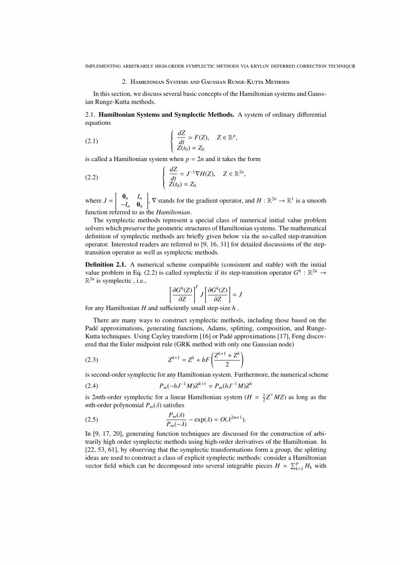
2.1. Hamiltonian Systems and Symplectic Methods. A system of ordinary differentialequations
(2.1)
dZdt
= F(Z), Z ∈ Rp,
Z(t0) = Z0
is called a Hamiltonian system when p = 2n and it takes the form
(2.2)
dZdt
= J−1∇H(Z), Z ∈ R2n,
Z(t0) = Z0
where J =
[0n In
−In 0n
], ∇ stands for the gradient operator, and H : R2n → R1 is a smooth
function referred to as the Hamiltonian.The symplectic methods represent a special class of numerical initial value problem
solvers which preserve the geometric structures of Hamiltonian systems. The mathematicaldefinition of symplectic methods are briefly given below via the so-called step-transitionoperator. Interested readers are referred to [9, 16, 31] for detailed discussions of the step-transition operator as well as symplectic methods.
Definition 2.1. A numerical scheme compatible (consistent and stable) with the initialvalue problem in Eq. (2.2) is called symplectic if its step-transition operator Gh : R2n →R2n is symplectic , i.e., [
∂Gh(Z)∂Z
]T
J[∂Gh(Z)∂Z
]= J
for any Hamiltonian H and sufficiently small step-size h .
There are many ways to construct symplectic methods, including those based on thePade approximations, generating functions, Adams, splitting, composition, and Runge-Kutta techniques. Using Cayley transform [16] or Pade approximations [17], Feng discov-ered that the Euler midpoint rule (GRK method with only one Gaussian node)
(2.3) Zk+1 = Zk + hF(
Zk+1 + Zk
2
)
is second-order symplectic for any Hamiltonian system. Furthermore, the numerical scheme
(2.4) Pm(−hJ−1M)Zk+1 = Pm(hJ−1M)Zk
is 2mth-order symplectic for a linear Hamiltonian system (H = 12 Z>MZ) as long as the
mth-order polynomial Pm(λ) satisfies
(2.5)Pm(λ)
Pm(−λ)− exp(λ) = O(λ2m+1).
In [9, 17, 20], generating function techniques are discussed for the construction of arbi-trarily high order symplectic methods using high-order derivatives of the Hamiltonian. In[22, 53, 61], by observing that the symplectic transformations form a group, the splittingideas are used to construct a class of explicit symplectic methods: consider a Hamiltonianvector field which can be decomposed into several integrable pieces H =
∑pk=1 Hk with

4 Q.D. FENG, N.M. NIE, J.F. HUANG, Z.J. SHANG, AND Y.F. TANG
phase flows qhk , one can easily obtain first-order and second-order symplectic schemes for
the original Hamiltonian H as in qhp ◦ · · · ◦ qh
2 ◦qh1 and qh/2
1 ◦ · · · ◦ qh/2p−1 ◦qh
p ◦qh/2p−1 ◦ · · · ◦ qh/2
1 ,respectively; and, higher-order schemes can be iteratively constructed by observing that ifqh is a symplectic scheme of order p, then qαh ◦qβh ◦qαh is also symplectic with order p+2when
α =1
2 − 21/(p+1) , β = − 21/(p+1)
2 − 21/(p+1) .
For the classical general linear schemes, it was shown that all linear multi-step schemes arenon-symplectic [29, 54], and with the exception of the trapezoid rule, all linear multi-stepmethods are even not conjugate-symplectic [21]. Therefore, for efficiency and stabilityconsiderations, one likes to use symplectic schemes based on the Runge-Kutta methods.The symplectic Runge-Kutta methods are Runge-Kutta methods
(2.6)
Zk+1 = Zk + hs∑
i=1biF(Yi),
Yi = Zk + hs∑
i=1ai jF(Y j), 1 ≤ i ≤ s
in which the coefficients satisfy the conditions
(2.7) bib j − biai j − b ja ji = 0, i, j = 1, 2, · · · , s,as discussed in [40, 46, 52].
We want to mention that in general it is hard to construct symplectic schemes using (2.6)and (2.7). In the following section, we introduce a special class of symplectic Runge-Kuttamethods based on the collocation formulation and Gaussian quadrature nodes.
2.2. Collocation and Gaussian Runge-Kutta Methods. The collocation methods arewidely used for the solution of differential equations. For a general ODE initial valuesystem in Eq. (2.1), given the stepsize h and a set of s distinct real numbers c1, · · · ,cs with 0 ≤ c j ≤ 1, the collocation method searches collocation polynomials Φ(t) =
[φ1(t), φ2(t), · · · , φ2n(t)]> of degree s satisfying{
Φ(t0 + c jh) = F(t0 + c jh,Φ(t0 + c jh)), j = 1, · · · , s.Φ(t0) = Z0.
(2.8)
The solution at t0 + h is then approximated by Z1 = Φ(t0 + h) [31].In [27, 59], it was shown that the collocation method is equivalent to the s-stage Runge-
Kutta method
Z1 = Z0 + hs∑
j=1b jK j,
K j = F(t0 + c jh,Z0 + h
s∑m=1
a jmKm
), j = 1, · · · , s,
where
(2.9) a jm =
∫ c j
0Lm(τ)dτ, b j =
∫ 1
0L j(τ)dτ,
and Lm(τ) is the Lagrange interpolating polynomial Lm(τ) =∏l,m
(τ − cl)/(cm − cl). Also, if
the conditionss∑
j=1
b jck−1j =
1k, k = 1, · · · , p
IMPLEMENTING ARBITRARILY HIGH-ORDER SYMPLECTIC METHODS VIA KRYLOV DEFERRED CORRECTION TECHNIQUE5
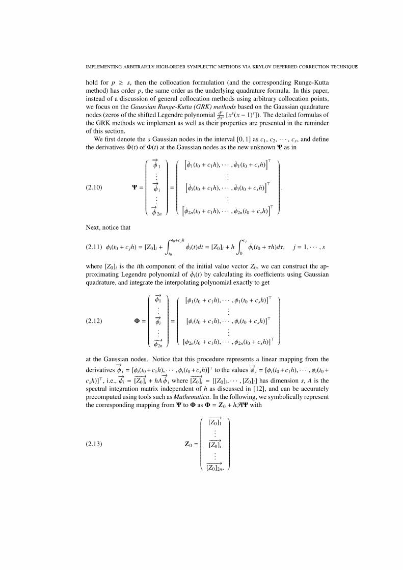
hold for p ≥ s, then the collocation formulation (and the corresponding Runge-Kuttamethod) has order p, the same order as the underlying quadrature formula. In this paper,instead of a discussion of general collocation methods using arbitrary collocation points,we focus on the Gaussian Runge-Kutta (GRK) methods based on the Gaussian quadraturenodes (zeros of the shifted Legendre polynomial ds
dxs [xs(x − 1)s]). The detailed formulas ofthe GRK methods we implement as well as their properties are presented in the reminderof this section.
We first denote the s Gaussian nodes in the interval [0, 1] as c1, c2, · · · , cs, and definethe derivatives Φ(t) of Φ(t) at the Gaussian nodes as the new unknown Ψ as in
Ψ =
−→φ 1...−→φ i...−→φ 2n
=
[φ1(t0 + c1h), · · · , φ1(t0 + csh)
]>...[
φi(t0 + c1h), · · · , φi(t0 + csh)]>
...[φ2n(t0 + c1h), · · · , φ2n(t0 + csh)
]>
.(2.10)
Next, notice that
(2.11) φi(t0 + c jh) = [Z0]i +
∫ t0+c jh
t0φi(t)dt = [Z0]i + h
∫ c j
0φi(t0 + τh)dτ, j = 1, · · · , s
where [Z0]i is the ith component of the initial value vector Z0, we can construct the ap-proximating Legendre polynomial of φi(t) by calculating its coefficients using Gaussianquadrature, and integrate the interpolating polynomial exactly to get
Φ =
−→φ1...−→φi...−−→φ2n
=
[φ1(t0 + c1h), · · · , φ1(t0 + csh)
]>...[
φi(t0 + c1h), · · · , φi(t0 + csh)]>
...[φ2n(t0 + c1h), · · · , φ2n(t0 + csh)
]>
(2.12)
at the Gaussian nodes. Notice that this procedure represents a linear mapping from the
derivatives−→φ i = [φi(t0 +c1h), · · · , φi(t0 +csh)]> to the values
−→φ i = [φi(t0 +c1h), · · · , φi(t0 +
csh)]>, i.e.,−→φi =
−−−→[Z0]i + hA
−→φ i where
−−−→[Z0]i = [[Z0]i, · · · , [Z0]i] has dimension s, A is the
spectral integration matrix independent of h as discussed in [12], and can be accuratelyprecomputed using tools such as Mathematica. In the following, we symbolically representthe corresponding mapping from Ψ to Φ as Φ = Z0 + hAΨ with
Z0 =
−−−→[Z0]1...−−−→
[Z0]i...−−−−→
[Z0]2n,
(2.13)
6 Q.D. FENG, N.M. NIE, J.F. HUANG, Z.J. SHANG, AND Y.F. TANG
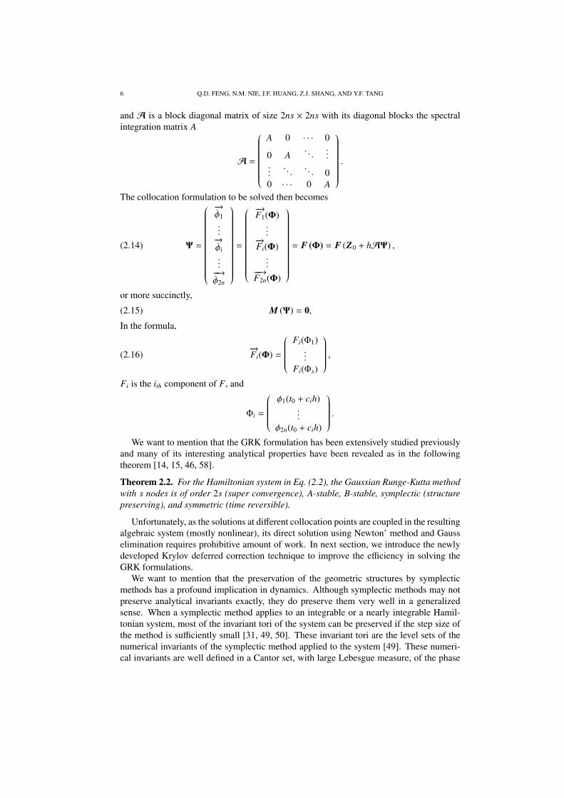
and A is a block diagonal matrix of size 2ns × 2ns with its diagonal blocks the spectralintegration matrix A
A =
A 0 · · · 0
0 A. . .
......
. . .. . . 0
0 · · · 0 A
.
The collocation formulation to be solved then becomes
(2.14) Ψ =
−→φ1...−→φi...−−→φ2n
=
−→F1(Φ)...−→
Fi(Φ)...−−→
F2n(Φ)
= F (Φ) = F (Z0 + hAΨ) ,
or more succinctly,
(2.15) M (Ψ) = 0,In the formula,
(2.16)−→Fi(Φ) =
Fi(Φ1)...
Fi(Φs)
,
Fi is the ith component of F, and
Φi =
φ1(t0 + cih)...
φ2n(t0 + cih)
.
We want to mention that the GRK formulation has been extensively studied previouslyand many of its interesting analytical properties have been revealed as in the followingtheorem [14, 15, 46, 58].
Theorem 2.2. For the Hamiltonian system in Eq. (2.2), the Gaussian Runge-Kutta methodwith s nodes is of order 2s (super convergence), A-stable, B-stable, symplectic (structurepreserving), and symmetric (time reversible).
Unfortunately, as the solutions at different collocation points are coupled in the resultingalgebraic system (mostly nonlinear), its direct solution using Newton’ method and Gausselimination requires prohibitive amount of work. In next section, we introduce the newlydeveloped Krylov deferred correction technique to improve the efficiency in solving theGRK formulations.
We want to mention that the preservation of the geometric structures by symplecticmethods has a profound implication in dynamics. Although symplectic methods may notpreserve analytical invariants exactly, they do preserve them very well in a generalizedsense. When a symplectic method applies to an integrable or a nearly integrable Hamil-tonian system, most of the invariant tori of the system can be preserved if the step size ofthe method is sufficiently small [31, 49, 50]. These invariant tori are the level sets of thenumerical invariants of the symplectic method applied to the system [49]. These numeri-cal invariants are well defined in a Cantor set, with large Lebesgue measure, of the phase
IMPLEMENTING ARBITRARILY HIGH-ORDER SYMPLECTIC METHODS VIA KRYLOV DEFERRED CORRECTION TECHNIQUE7
space and approximate the exact invariants of the system with order of accuracy equal tothat of the method [49]. Backward error analysis shows that the numerical orbits of a sym-plectic method approximate the exact orbits of some perturbed Hamiltonian system verywell during a very long interval of iteration steps (exponentially long in 1/h where h is thestep size) [31]. For the GRK methods, assuming the discretized collocation formulationis solved exactly, it has been proven that all the quadratic invariants are exactly preservedin the numerical simulation [19, 31]. Non-quadratic invariants, as we will show later, areusually not exactly preserved and, as remarked above, can still be used as measures of thesolution error in the numerical simulation when analytical formulas are not available.
3. K D C T
To solve the nonlinear system in Eq. (2.15), classical Newton’s method can be employedto iteratively refine the approximate solution using
(3.1) Ψ[n+1] = Ψ[n] − δ[n]
where δ[n] solves the linear approximation of the error equation given by
(3.2) JM(Ψ[n]
)δ[n] = M
(Ψ[n]
),
and JM(Ψ[n]
)is the Jacobian of M (Ψ) at Ψ[n]. As JM
(Ψ[n]
)is in general a dense matrix,
solving Eq. (3.2) using direct Gaussian elimination requires prohibitive O((2ns)3) opera-tions, which becomes extremely expensive for large s. Therefore, most existing implemen-tations of the GRK methods are limited to order up to 10 (s = 5) or so.
An alternative class of methods for solving Eq. (3.2) iteratively searches the optimalsolution in the Krylov subspace defined by
(3.3) Kk
(JM, M
(Ψ[n]
))=
{M
(Ψ[n]
), JM M
(Ψ[n]
), · · · , Jk−1
M M(Ψ[n]
)}.
Consider the case where the Jacobian matrix is of the form
(3.4) JM(Ψ[n]
)= ±I −C,
and most eigenvalues of C are clustered at 0. As the numerical rank of the correspondingKrylov subspace is low, it is not hard to see that the solution converges to a prescribedaccuracy after a few Krylov iterations and the resulting Krylov subspace method can beextremely efficient. Further notice that to solve the nonlinear equation (2.15), it is notnecessary to solve Eq. (3.2) exactly during each Newton iteration, therefore the Newtoniteration can be resumed once the residual in Eq. (3.2) is reduced by a prescribed factor inthe Krylov subspace methods. The resulting methods are usually referred to as the Newton-Krylov methods [36, 37, 45]. In summary, an efficient implementation of the Newton-Krylov method requires
(a) the Jacobian matrix of the nonlinear system be close to the identity matrix I andhence well-conditioned, and
(b) an efficient procedure to compute the matrix vector product JM M(Ψ[n]).For (a), a common practice to derive well-conditioned system is to introduce precondi-
tioners to the original equation. Traditionally, the inverse of a sparse matrix close to theoriginal system has been widely used as preconditioner in numerical linear algebra. Morerecent results include integral operators as preconditioners which can be applied efficientlyto any vector using fast convolution algorithms such as the fast multipole methods or theprecorrected FFT [26, 44]. In this paper, we utilize the Krylov deferred correction tech-nique which uses a lower order explicit or implicit method to precondition the higher order
8 Q.D. FENG, N.M. NIE, J.F. HUANG, Z.J. SHANG, AND Y.F. TANG
implicit GRK formulations and decouple the equation at different collocation nodes. Sim-ilar to deferred or defect correction schemes, we first assume a provisional solution to thecollocation formulation (2.15) is derived using a low order marching scheme (such as theforward Euler or low order Runge-Kutta methods) and denote it by
Ψ[0] =
−→ψ1
[0]
...−−→ψ2n
[0]
,
where the vectors represent the solutions for each component at different collocation nodesas given by
−→ψi
[0] =
ψ[0]i (t1)...
ψ[0]i (ts)
, i = 1, · · · , 2n.
As Gaussian nodes are used as the interpolation points, we can calculate the coefficients ofthe degree s − 1 interpolating polynomials
Ψ[0](t) =
ψ[0]1 (t)...
ψ[0]2n (t)
using Gaussian quadratures and fast Legendre transform [13], and define the error as
(3.5)−→δ (t) =
δ1(t)...
δ2n(t)
=
ψ1(t)...
ψ2n(t)
−
ψ[0]1 (t)...
ψ[0]2n (t)
.
The discretized error equation is then simply
(3.6) δ = F(Z0 + hAΨ[0] + hAδ
)−Ψ[0],
where δ = (δ1(t1), · · · , δ1(ts), · · · , δ2n(t1), · · · , δ2n(ts))>.Next, similar to the deferred correction schemes, a low order method can be used to
solve the error equation. In [33], it was shown that the low order method is equivalent toapplying a lower triangular matrix to approximate the integral operator and the spectralintegration matrix A, in particular, the forward Euler’s method is equivalent to the rectan-gular rule using left end-point and the backward Euler’s method the rectangular rule usingthe right end-point. Hence the low order method solves the discretized system
(3.7) δ = F(Z0 + hAΨ[0] + hAδ
)−Ψ[0],
where A is the low order approximation of the spectral integration operator A and δ thelow order approximation of the error δ. We can succinctly write Eq. (3.7) as an explicitfunction
(3.8) δ = M(Ψ[0]
).
Notice that when Ψ[0] solves the GRK collocation formulation in Eq. (2.15), we haveδ = 0. Therefore, solving Eq. (2.15) is equivalent to finding the zero of M. Using theimplicit function theorem, the Jacobian of M can be easily derived as
J M =∂δ
∂Ψ[0] = −(I − hJFA
)−1(I − hJFA) .
IMPLEMENTING ARBITRARILY HIGH-ORDER SYMPLECTIC METHODS VIA KRYLOV DEFERRED CORRECTION TECHNIQUE9
As both hA and hA are approximations of the integral operator, it is not surprising that forreasonable small h, the two matrices are close and the Jacobian matrix J M is hence veryclose to −I , i.e., the preconditioned equation
M(Ψ[0]
)= 0
is better conditioned, hence the Newton-Krylov methods quickly converge to the pre-scribed accuracy requirement. For comparison, the Jacobian of M is given by
JM = hJFA − I .
As for (b), one can either formulate the Jacobian matrix of M explicitly if possible, orapply the Jacobian free technique where the matrix vector product is approximated by aforward difference formula, i.e., for any vector v, JM(x)v is approximated by
DτM(x : v) =M(x + τv) − M(x)
τ
for some properly chosen parameter τ [37]. Notice that the evaluation of M is simply onelow order solution of the error equation and hence can be very efficient. Our numericalexperiments show that the Jacobian free techniques are more efficient during each Kryloviteration, while the explicit formula utilizing the analytical Jacobian matrix provides betterconvergence behavior in the Newton-Krylov methods because of its improved accuracy.The implementation details of the Newton-Krylov methods are still being studied by theauthors and results will be reported in the future.
Finally in this section, we want to mention that most of the techniques we use havebeen studied previously. Hence many of the technical details are neglected in this paperand we refer interested readers to [36, 37] for further discussions of the Newton-Krylovtechniques, to [38] for an interesting summary of existing Jacobian free Newton-Krylovmethods, to [12, 13] for the spectral deferred correction methods and how the spectralintegration matrix and error equation are computed, and to [33, 34] for a detailed discussionof the Krylov deferred correction methods for general differential algebraic equations.
4. N R
In this section, we study the performance of the GRK methods with different orders,and compare the symplectic methods with non-symplectic ones in efficiency and invariantpreservation.
4.1. Hamiltonian Systems. Our numerical experiments focus on three Hamiltonian sys-tems: the harmonic oscillator, Kepler motion, and geodesic flow on ellipsoid, which repre-sent the linear, semi-linear and non-linear Hamiltonian systems, respectively.
Harmonic OscillatorThe harmonic oscillator is a simple linear Hamiltonian system which describes the mo-
tion of a mass point controlled by an elastic spring. It is given by the equationsdpdt
= −q
dqdt
= p,
where the Hamiltonian function is defined as H = 12 (p2 + q2).
10 Q.D. FENG, N.M. NIE, J.F. HUANG, Z.J. SHANG, AND Y.F. TANG
Kepler MotionThe Kepler motion is a semi-linear Hamiltonian system modeling the movement of
celestial bodies. It is usually given by
p1 = − q1
(q21 + q2
2)3/2, q1 = p1,
p2 = − q2
(q21 + q2
2)3/2, q2 = p2,
where the Hamiltonian function is defined as H = 12 (p2
1 + p22) − 1/
√q2
1 + q22. For this
system, both the Hamiltonian and angular momentum L = q1 p2 − q2 p1 are invariants.As the orbit of the Kepler motion is an ellipse, we choose the initial values p1(0) = 0,
p2(0) = 2, q1(0) = 0.4, and q2(0) = 0 so that the fundamental period of the motion isT = 2π (see [1, 31]). We present simulation results for approximately 100 periods in theinterval [0, 630].
Geodesic Flow on EllipsoidOur last example considers the geodesic flow on the ellipsoid with three major axes of
different lengths (a, b, c), which models the motion of a unit-mass point on the surface ofthe ellipsoid without any external forces. The corresponding Hamiltonian is
(4.1) H(p1, p2; q1, q2) =g22 p2
1 − 2g12 p1 p2 + g11 p22
2|G| ,
where
g11 = cos2 q1
(a2 cos2 q2 + b2 sin2 q2
)+ c2 sin2 q1,
g12 =14
(b2 − a2) sin 2q1 sin 2q2,
g22 = sin2 q1(a2 sin2 q2 + b2 cos2 q2),
and G is a symmetric matrix(
g11 g12g12 g22
)with determinant |G| = g11g22−g2
12. It is shown
in ([55]) that in addition to the Hamiltonian, the quantity
(4.2) A(p1, p2, q1, q2) = g11 +g22
sin2 q1− p2
1
13.5− p2
2
13.5 sin2 q1
also represents an invariant. In the simulation, we set a = 9.5, b = 5.5, c = 2.5, and choosethe initial values p1(0) = 8.846945, q1(0) = π/2, p2(0) = 5.436522, and q2(0) = 0.
4.2. Symplectic Methods with Different Orders. Traditionally, symplectic methods havebeen limited to lower orders due to reasons discussed in previous sections. Here, we com-pare the performance of the KDC accelerated GRK methods with different number ofGaussian nodes s = 2, 4, 6, 8, 10, which correspond to orders 4, 8, 12, 16, 20, respectively.Our numerical code is written in matlab.
For each s in our numerical experiments, we compare the accuracy(for different step-size) as a function of the CPU time (which is approximately equivalent to the total amountof operations). For the harmonic oscillator problem, as the analytical solution is known,we plot the real error in Figure 1. Similar results can be derived for the Kepler motionproblem as shown in Figure 2. However, as the analytical solution is not readily availablefor this problem, we measure the error after each period where the exact solution should bep1 = 0, q1 = 0.4, p2 = 2, q2 = 0, the same as the initial condition. Finally for the geodesic
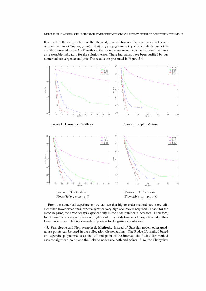
IMPLEMENTING ARBITRARILY HIGH-ORDER SYMPLECTIC METHODS VIA KRYLOV DEFERRED CORRECTION TECHNIQUE11
flow on the Ellipsoid problem, neither the analytical solution nor the exact period is known.As the invariants H(p1, p2, q1, q2) and A(p1, p2, q1, q2) are not quadratic, which can not beexactly preserved by the GRK methods, therefore we measure the errors in these invariantsas reasonable indicators for the solution error. These indicators have been verified by ournumerical convergence analysis. The results are presented in Figure 3-4.
0 10 20 30 40 50 60 70 80 90 10010
−15
10−10
10−5
100
cpu time
max
err
or
4−ord8−ord12−ord16−ord20−ord
F 1. Harmonic Oscillator
0 100 200 300 400 500 60010
−12
10−10
10−8
10−6
10−4
10−2
100
cpu time
max
err
or
4−ord8−ord12−ord16−ord20−ord
F 2. Kepler Motion
0 50 100 150 200 250 300 350 400 450 50010
−12
10−10
10−8
10−6
10−4
10−2
100
cpu time
Ham
ilton
ian
erro
r
4−ord8−ord12−ord16−ord20−ord
F 3. GeodesicFlows(H(p1, p2, q1, q2))
0 50 100 150 200 250 30010
−12
10−10
10−8
10−6
10−4
10−2
100
cpu time
A−
erro
r
4−ord8−ord12−ord16−ord20−ord
F 4. GeodesicFlows(A(p1, p2, q1, q2))
From the numerical experiments, we can see that higher order methods are more effi-cient than lower order ones, especially when very high accuracy is required. In fact, for thesame stepsize, the error decays exponentially as the node number s increases. Therefore,for the same accuracy requirement, higher order methods take much larger time-step thanlower order ones. This is extremely important for long-time simulations.
4.3. Symplectic and Non-symplectic Methods. Instead of Gaussian nodes, other quad-rature points can be used in the collocation discretizations. The Radau IA method basedon Legendre polynomial uses the left end point of the interval, the Radau IIA methoduses the right end point, and the Lobatto nodes use both end points. Also, the Chebyshev
12 Q.D. FENG, N.M. NIE, J.F. HUANG, Z.J. SHANG, AND Y.F. TANG
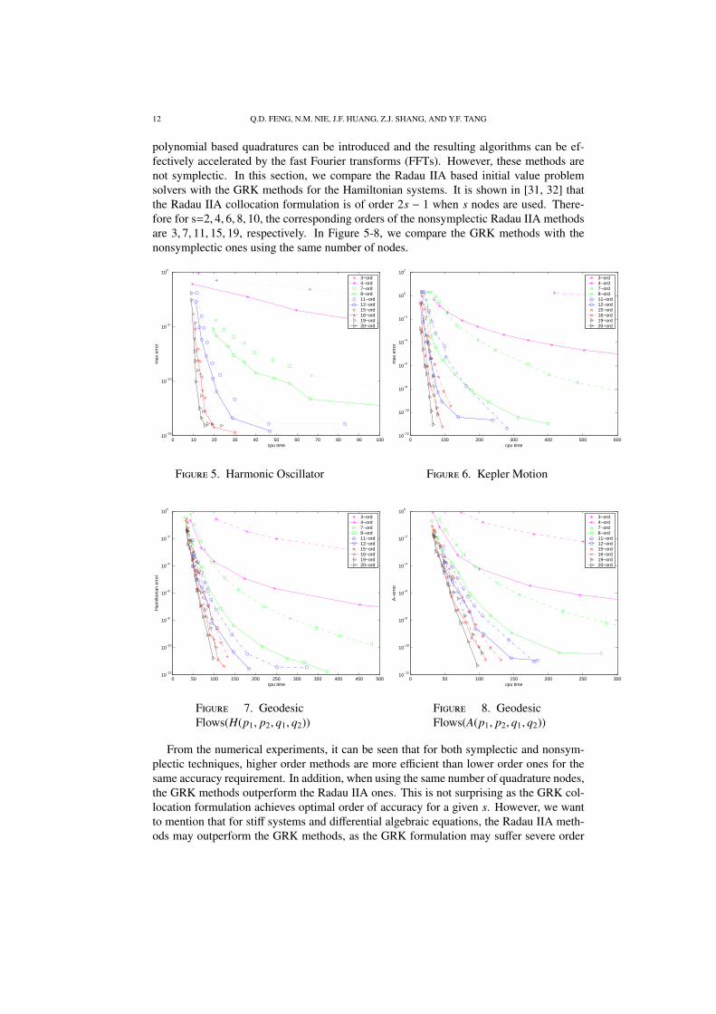
polynomial based quadratures can be introduced and the resulting algorithms can be ef-fectively accelerated by the fast Fourier transforms (FFTs). However, these methods arenot symplectic. In this section, we compare the Radau IIA based initial value problemsolvers with the GRK methods for the Hamiltonian systems. It is shown in [31, 32] thatthe Radau IIA collocation formulation is of order 2s − 1 when s nodes are used. There-fore for s=2, 4, 6, 8, 10, the corresponding orders of the nonsymplectic Radau IIA methodsare 3, 7, 11, 15, 19, respectively. In Figure 5-8, we compare the GRK methods with thenonsymplectic ones using the same number of nodes.
0 10 20 30 40 50 60 70 80 90 10010
−15
10−10
10−5
100
cpu time
max
err
or
3−ord4−ord7−ord8−ord11−ord12−ord15−ord16−ord19−ord20−ord
F 5. Harmonic Oscillator
0 100 200 300 400 500 60010
−12
10−10
10−8
10−6
10−4
10−2
100
102
cpu time
max
err
or
3−ord4−ord7−ord8−ord11−ord12−ord15−ord16−ord19−ord20−ord
F 6. Kepler Motion
0 50 100 150 200 250 300 350 400 450 50010
−12
10−10
10−8
10−6
10−4
10−2
100
cpu time
Ham
ilton
ian
erro
r
3−ord4−ord7−ord8−ord11−ord12−ord15−ord16−ord19−ord20−ord
F 7. GeodesicFlows(H(p1, p2, q1, q2))
0 50 100 150 200 250 30010
−12
10−10
10−8
10−6
10−4
10−2
100
cpu time
A−
erro
r
3−ord4−ord7−ord8−ord11−ord12−ord15−ord16−ord19−ord20−ord
F 8. GeodesicFlows(A(p1, p2, q1, q2))
From the numerical experiments, it can be seen that for both symplectic and nonsym-plectic techniques, higher order methods are more efficient than lower order ones for thesame accuracy requirement. In addition, when using the same number of quadrature nodes,the GRK methods outperform the Radau IIA ones. This is not surprising as the GRK col-location formulation achieves optimal order of accuracy for a given s. However, we wantto mention that for stiff systems and differential algebraic equations, the Radau IIA meth-ods may outperform the GRK methods, as the GRK formulation may suffer severe order
IMPLEMENTING ARBITRARILY HIGH-ORDER SYMPLECTIC METHODS VIA KRYLOV DEFERRED CORRECTION TECHNIQUE13
reduction and hence have lower B-convergence orders. The readers are referred to [32] forB-convergence and order reductions for different collocation formulations.
4.4. Preserving the Invariants. One advantage of the symplectic methods is their abilityto better preserve the invariants of the Hamiltonian systems. In this section, we comparethe accuracy of the symplectic and nonsymplectic methods in both the invariants and thesolution itself. We want to mention that for many Hamiltonian systems, as the analyticalsolution is not readily available, one possible measure of the numerical error is to checkhow these invariants change as a function of time. However, such strategy may not workwell for symplectic methods, especially when the invariants are preserved exactly by thenumerical discretizations, as in the harmonic oscillator(Hamiltonian) and Kepler motion(angular momentum) problems. We also want to mention that when different sources oferrors are considered, in particular, the error in solving the collocation formulations, theGRK methods can not preserve the invariants exactly. In the following, we show how theinvariants change as a function of time for different methods and different systems.
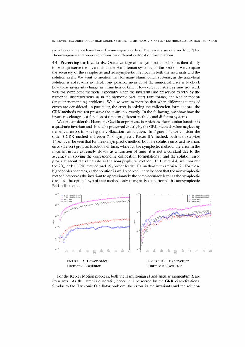
We first consider the Harmonic Oscillator problem, in which the Hamiltonian function isa quadratic invariant and should be preserved exactly by the GRK methods when neglectingnumerical errors in solving the collocation formulation. In Figure 4.4, we consider theorder 8 GRK method and order 7 nonsymplectic Radau IIA method, both with stepsize1/16. It can be seen that for the nonsymplectic method, both the solution error and invarianterror (Herror) grow as functions of time, while for the symplectic method, the error in theinvariant grows extremely slowly as a function of time (it is not a constant due to theaccuracy in solving the corresponding collocation formulations), and the solution errorgrows at about the same rate as the nonsymplectic method. In Figure 4.4, we considerthe 20th order GRK method and 19th order Radau IIa method with stepsize 2. For thesehigher order schemes, as the solution is well resolved, it can be seen that the nonsymplecticmethod preserves the invariant to approximately the same accuracy level as the symplecticone, and the optimal symplectic method only marginally outperforms the nonsymplecticRadau IIa method.
0 100 200 300 400 500 600 700 800 900 100010
−16
10−15
10−14
10−13
10−12
10−11
time
erro
r
8−ord Hamiltonian error7−ord Hamiltonian error8−ord error7−ord error
F 9. Lower-orderHarmonic Oscillator
0 100 200 300 400 500 600 700 800 900 100010
−16
10−15
10−14
10−13
time
erro
r
20−ord Hamiltonian error19−ord Hamiltonian error20−ord error19−ord error
F 10. Higher-orderHarmonic Oscillator
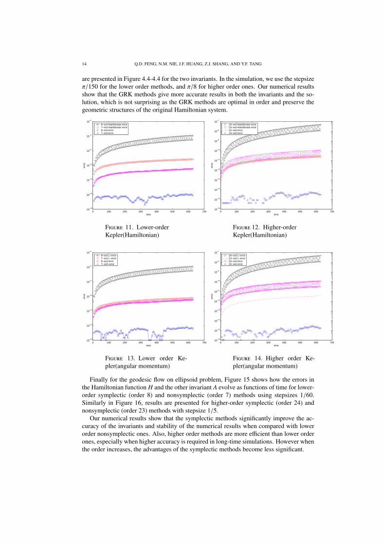
For the Kepler Motion problem, both the Hamiltonian H and angular momentum L areinvariants. As the latter is quadratic, hence it is preserved by the GRK discretizations.Similar to the Harmonic Oscillator problem, the errors in the invariants and the solution
14 Q.D. FENG, N.M. NIE, J.F. HUANG, Z.J. SHANG, AND Y.F. TANG
are presented in Figure 4.4-4.4 for the two invariants. In the simulation, we use the stepsizeπ/150 for the lower order methods, and π/8 for higher order ones. Our numerical resultsshow that the GRK methods give more accurate results in both the invariants and the so-lution, which is not surprising as the GRK methods are optimal in order and preserve thegeometric structures of the original Hamiltonian system.
0 100 200 300 400 500 600 70010
−16
10−14
10−12
10−10
10−8
10−6
10−4
time
erro
r
8−ord Hamiltonian error7−ord Hamiltonian error8−ord error7−ord error
F 11. Lower-orderKepler(Hamiltonian)
0 100 200 300 400 500 600 70010
−16
10−15
10−14
10−13
10−12
10−11
10−10
10−9
10−8
10−7
timeer
ror
24−ord Hamiltonian error23−ord Hamiltonian error24−ord error23−ord error
F 12. Higher-orderKepler(Hamiltonian)
0 100 200 300 400 500 600 70010
−16
10−14
10−12
10−10
10−8
10−6
10−4
time
erro
r
8−ord L−error7−ord L−error8−ord error7−ord−error
F 13. Lower order Ke-pler(angular momentum)
0 100 200 300 400 500 600 70010
−16
10−15
10−14
10−13
10−12
10−11
10−10
10−9
10−8
10−7
time
erro
r
24−ord L−error23−ord L−error24−ord error23−ord error
F 14. Higher order Ke-pler(angular momentum)
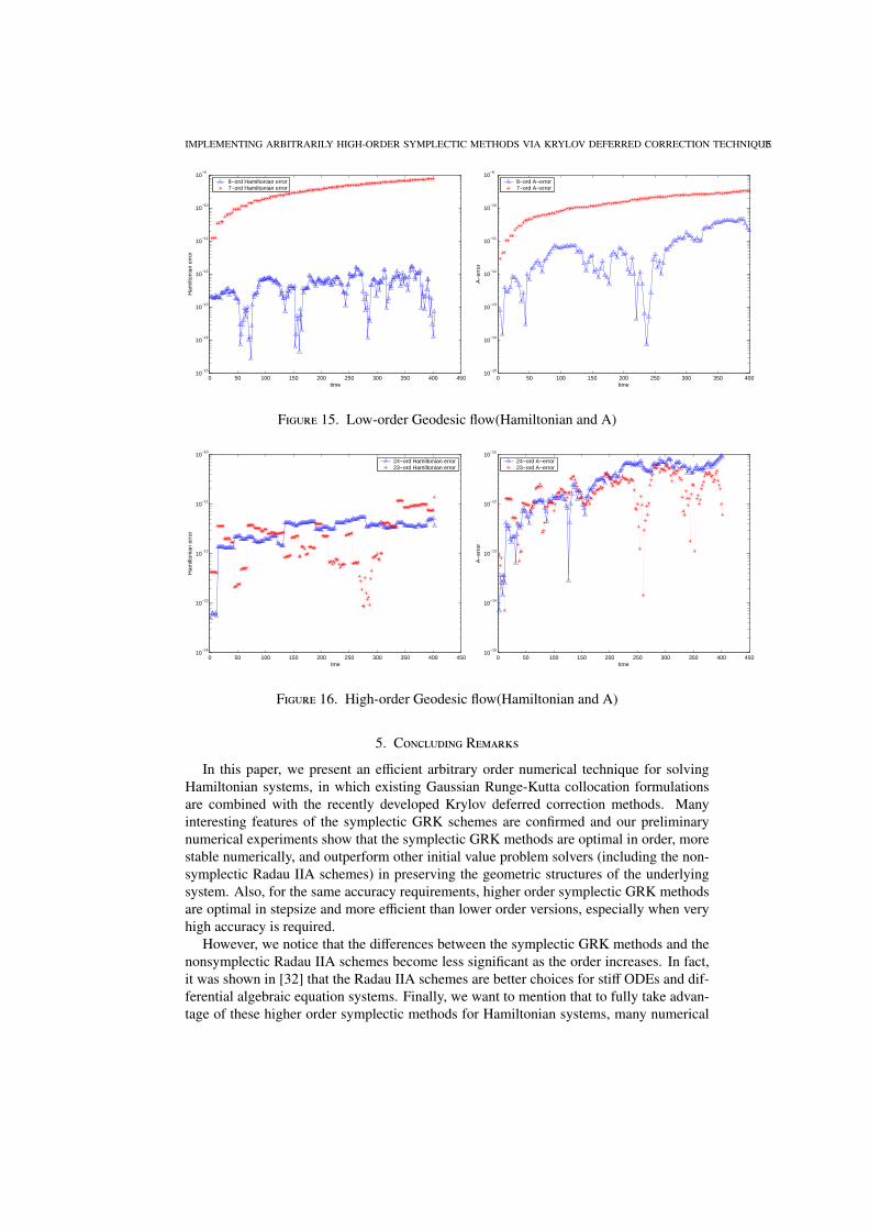
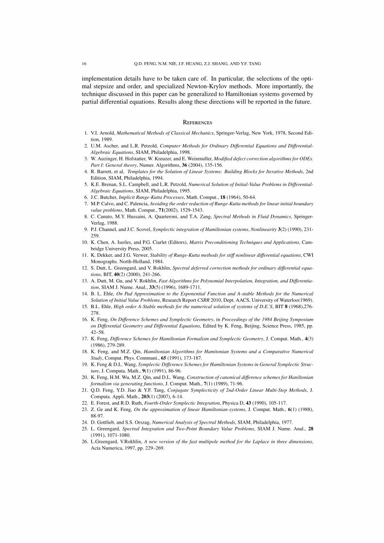
Finally for the geodesic flow on ellipsoid problem, Figure 15 shows how the errors inthe Hamiltonian function H and the other invariant A evolve as functions of time for lower-order symplectic (order 8) and nonsymplectic (order 7) methods using stepsizes 1/60.Similarly in Figure 16, results are presented for higher-order symplectic (order 24) andnonsymplectic (order 23) methods with stepsize 1/5.
Our numerical results show that the symplectic methods significantly improve the ac-curacy of the invariants and stability of the numerical results when compared with lowerorder nonsymplectic ones. Also, higher order methods are more efficient than lower orderones, especially when higher accuracy is required in long-time simulations. However whenthe order increases, the advantages of the symplectic methods become less significant.
IMPLEMENTING ARBITRARILY HIGH-ORDER SYMPLECTIC METHODS VIA KRYLOV DEFERRED CORRECTION TECHNIQUE15
0 50 100 150 200 250 300 350 400 45010
−15
10−14
10−13
10−12
10−11
10−10
10−9
time
Ham
ilton
ian
erro
r8−ord Hamiltonian error7−ord Hamiltonian error
0 50 100 150 200 250 300 350 40010
−15
10−14
10−13
10−12
10−11
10−10
10−9
time
A−
erro
r
8−ord A−error7−ord A−error
F 15. Low-order Geodesic flow(Hamiltonian and A)
0 50 100 150 200 250 300 350 400 45010
−14
10−13
10−12
10−11
10−10
tme
Ham
ilton
ian
erro
r
24−ord Hamiltonian error23−ord Hamiltonian error
0 50 100 150 200 250 300 350 400 45010
−15
10−14
10−13
10−12
10−11
time
A−
erro
r
24−ord A−error23−ord A−error
F 16. High-order Geodesic flow(Hamiltonian and A)
5. C R
In this paper, we present an efficient arbitrary order numerical technique for solvingHamiltonian systems, in which existing Gaussian Runge-Kutta collocation formulationsare combined with the recently developed Krylov deferred correction methods. Manyinteresting features of the symplectic GRK schemes are confirmed and our preliminarynumerical experiments show that the symplectic GRK methods are optimal in order, morestable numerically, and outperform other initial value problem solvers (including the non-symplectic Radau IIA schemes) in preserving the geometric structures of the underlyingsystem. Also, for the same accuracy requirements, higher order symplectic GRK methodsare optimal in stepsize and more efficient than lower order versions, especially when veryhigh accuracy is required.
However, we notice that the differences between the symplectic GRK methods and thenonsymplectic Radau IIA schemes become less significant as the order increases. In fact,it was shown in [32] that the Radau IIA schemes are better choices for stiff ODEs and dif-ferential algebraic equation systems. Finally, we want to mention that to fully take advan-tage of these higher order symplectic methods for Hamiltonian systems, many numerical
16 Q.D. FENG, N.M. NIE, J.F. HUANG, Z.J. SHANG, AND Y.F. TANG
implementation details have to be taken care of. In particular, the selections of the opti-mal stepsize and order, and specialized Newton-Krylov methods. More importantly, thetechnique discussed in this paper can be generalized to Hamiltonian systems governed bypartial differential equations. Results along these directions will be reported in the future.
R
1. V.I. Arnold, Mathematical Methods of Classical Mechanics, Springer-Verlag, New York, 1978, Second Edi-tion, 1989.
2. U.M. Ascher, and L.R. Petzold, Computer Methods for Ordinary Differential Equations and Differential-Algebraic Equations, SIAM, Philadelphia, 1998.
3. W. Auzinger, H. Hofstatter, W. Kreuzer, and E. Weinmuller, Modified defect correction algorithms for ODEs.Part I: General theory, Numer. Algorithms, 36 (2004), 135-156.
4. R. Barrett, et al, Templates for the Solution of Linear Systems: Building Blocks for Iterative Methods, 2ndEdition, SIAM, Philadelphia, 1994.
5. K.E. Brenan, S.L. Campbell, and L.R. Petzold, Numerical Solution of Initial-Value Problems in Differential-Algebraic Equations, SIAM, Philadelphia, 1995.
6. J.C. Butcher, Implicit Runge-Kutta Processes, Math. Comput., 18 (1964), 50-64.7. M.P. Calvo, and C. Palencia, Avoiding the order reduction of Runge-Kutta methods for linear initial boundary
value problems, Math. Comput., 71(2002), 1529-1543.8. C. Canuto, M.Y. Hussaini, A. Quarteroni, and T.A. Zang, Spectral Methods in Fluid Dynamics, Springer-
Verlag, 1988.9. P.J. Channel, and J.C. Scovel, Symplectic integration of Hamiltonian systems, Nonlinearity 3(2) (1990), 231-
259.10. K. Chen, A. Iserles, and P.G. Ciarlet (Editors), Matrix Preconditioning Techniques and Applications, Cam-
bridge University Press, 2005.11. K. Dekker, and J.G. Verwer, Stability of Runge-Kutta methods for stiff nonlinear differential equations, CWI
Monographs. North-Holland, 1984.12. S. Dutt, L. Greengard, and V. Rokhlin, Spectral deferred correction methods for ordinary differential equa-
tions, BIT, 40(2) (2000), 241-266.13. A. Dutt, M. Gu, and V. Rokhlin, Fast Algorithms for Polynomial Interpolation, Integration, and Differentia-
tion, SIAM J. Nume. Anal., 33(5) (1996), 1689-1711.14. B. L. Ehle, On Pad Approximation to the Exponential Function and A-stable Methods for the Numerical
Solution of Initial Value Problems, Research Report CSRR 2010, Dept. AACS, University of Waterloo(1969).15. B.L. Ehle, High order A-Stable methods for the numerical solution of systems of D.E.’S, BIT 8 (1968),276-
278.16. K. Feng, On Difference Schemes and Symplectic Geometry, in Proceedings of the 1984 Beijing Symposium
on Differential Geometry and Differential Equations, Edited by K. Feng, Beijing, Science Press, 1985, pp.42–58.
17. K. Feng, Difference Schemes for Hamiltonian Formalism and Symplectic Geometry, J. Comput. Math., 4(3)(1986), 279-289.
18. K. Feng, and M.Z. Qin, Hamiltonian Algorithms for Hamitonian Systems and a Comparative NumericalStudy, Comput. Phys. Communi., 65 (1991), 173-187.
19. K. Feng & D.L. Wang, Symplectic Difference Schemes for Hamiltonian Systems in General Symplectic Struc-ture, J. Computa. Math., 9(1) (1991), 86-96.
20. K. Feng, H.M. Wu, M.Z. Qin, and D.L. Wang, Construction of canonical difference schemes for Haniltonianformalism via generating functions, J. Comput. Math., 7(1) (1989), 71-96.
21. Q.D. Feng, Y.D. Jiao & Y.F. Tang, Conjugate Symplecticity of 2nd-Order Linear Multi-Step Methods, J.Computa. Appli. Math., 203(1) (2007), 6-14.
22. E. Forest, and R.D. Ruth, Fourth-Order Symplectic Integration, Physica D, 43 (1990), 105-117.23. Z. Ge and K. Feng, On the approximation of linear Hamiltonian-systems, J. Comput. Math., 6(1) (1988),
88-97.24. D. Gottlieb, and S.S. Orszag, Numerical Analysis of Spectral Methods, SIAM, Philadelphia, 1977.25. L. Greengard, Spectral Integration and Two-Point Boundary Value Problems, SIAM J. Nume. Anal., 28
(1991), 1071-1080.26. L.Greengard, V.Rokhlin, A new version of the fast multipole method for the Laplace in three dimensions,
Acta Numerica, 1997, pp. 229–269.
IMPLEMENTING ARBITRARILY HIGH-ORDER SYMPLECTIC METHODS VIA KRYLOV DEFERRED CORRECTION TECHNIQUE17
27. Guillou &J.L.Soule, La resolution numerique des problemes differentiels aux conditions initiales par desmethodes de collocation, Rev.Francaise Informat.Recherche Oprationnelle 3, Ser.R-3,17-44,[II.1],1969.
28. E. Hairer, and M. Hairer,”GniCodes - Matlab programs for geometric numerical integration”, Frontiers inNumerical Analysis (Durham 2002), Springer, Berlin, 2003.
29. E. Hairer & P. Leone, Order Barriers for Symplectic Multi-Value Methods, in: Numerical Analysis 1997, Pro-ceedings of the 17th Dundee Biennial Conference, June 24-27, 1997 (Edited by D.F. Griffiths, D.J. Highamand G.A. Watson), Pitman Research Notes in Mathematics Series Vol. 380, 1998, pp. 133-149.
30. E. Hairer, Ch. Lubich, and M. Roche, The Numerical Solution of Differential-Algebraic Systems by Runge-Kutta Methods, Springer-Verlag, 1989.
31. E. Hairer, Ch. Lubich, and G. Wanner, Geometric Numerical Integration, Springer, 2002.32. E. Hairer, and G. Wanner, Solving Ordinary Differential Equations II, Springer, 1996.33. J.F. Huang, J. Jia, and M. Minion, Accelerating the Convergence of Spectral Deferred Correction Methods,
J. Comput. Phys., 214(2) (2006), 633-656.34. J.F. Huang, J. Jia & M. Minion, Arbitrary Order Krylov Deferred Correction Methods for Differential Alge-
braic Equations, J. Comput. Phys., 221(2) (2007), 739-760.35. Hisashi Ishida, Yoshinori Nagai, and Akinori Kidera, Symplectic integrator for molecular dynamics of a
protein in water, Chemical Physics Letters, 282(2) (1998), 115-120.36. C.T. Kelly, Iterative Methods for Linear and Nonlinear Equations, SIAM, 1995.37. C.T. Kelly, Solving Nonlinear Equations with Newton’s Method, SIAM, 2003.38. D.A. Knoll, and D.E. Keyes, Jacobian-free Newton-Krylov methods: a survey of approaches and applica-
tions, J. Comput. Phys., 193 (2004), 357-397.39. M.P. Laburta, Construction of starting algorithms for the RK-Gauss methods, J. Comput Appl. Math., 90(2)
(1998), 239-261.40. F.M. Lasagni, Canonical Runge-Kutta Methods, ZAMP, 39(6) (1988), 952-953.41. A.T. Layton, and M.L. Minion, Conservative multi-implicit spectral deferred correction methods for reacting
gas dynamics, J. Comput. Phys., 194(2) (2004), 697C714.42. V. Pereyra, Iterated Deferred Correction for Nonlinear Boundary Value Problems, Numer. Math., 11 (1968),
111-125.43. L.R. Petzold, A Description of DASSL: A Differential-Algebraic System Solver, SAND82-8637, Sandia Na-
tional Lab, 1982.44. Joel R. Phillips and J. K. White, A precorrected-FFT method for electrostatic analysis of complicated 3D
structures, IEEE Transactions on Computer-Aided Design of Integrated Circuits and Systems, 1997, pp.1059–1072.
45. Y. Saad, and M.H. Schultz, GMRES: a generalized minimal residual algorithm for solving non-symmetriclinear systems, SIAM J. Sci. Stat. Comp., 7 (1986), 856–869.
46. J.M. Sanz-Serna, Runge-Kutta schemes for Hamiltonian systems, BIT, 28 (1998), 877-883.47. J.M. Sanz-Serna and M.P. Calvo, Numerical Hamiltonian Problems, Chapman & Hall, London, (1994).48. J.C. Scovel, Symplectic numerical integration of Hamiltonian systems, The Geometry of Hamiltonian Sys-
tems, MSRI Series, Vol. 22, (Edited by T.Ratiu), Springer-Verlag, New York, 1991, pp. 463-496.49. Z.J. Shang, KAM theorem of symplectic algorithms for Hamiltonian systems, Numer. Math., 83 (1999), 477-
496.50. Z.J. Shang, Resonant and Diophantine step sizes in computing invariant tori of Hamiltonian systems, Non-
linearity, 13 (2000), 299-308.51. J. Strain, Fast Stable Deferred Correction Methods for Two-Point Boundary Value Problems, Preprint.52. Y.B. Suris, On the preservation of the symplectic structure for numerical integration of Hamiltonian sys-
tems, Numerical Solution of Differential Equations, (Edited by S.S. Filippov), USSR Academy of Sciences,Moscow, 1988, pp. 148-160.
53. M. Suzuki, Fractal Decomposition of Exponential Operators with Applications to Many-Body Theories andMonte Carlo Simulations, Phys. Lett. A, 146(6) (1990), 319-323.
54. Y.F. Tang, The Symplecticity of Multi-Step Methods, Computers Math. Applic., 25(3) (1993), 83-90.55. Y.F. Tang, Geodesic Flows on Compact Surfaces—As an Application of Hamiltonian Formalism, Computers
Math. Applic., 26(1) (1993), 21-33.56. Y.F. Tang, J.W. Cao, X.T. Liu & Y.C. Sun, Symplectic methods for the Ablowitz-Ladik discrete nonlinear
Schrodinger equation, J. Phys. A: Math. Theor., 40 (2007), 2425-2437.57. L.N. Trefethen, and M.R. Trummer, An instability phenomenon in spectral methods, SIAM J. Numer. Anal.,
24 (1987).58. G. Wanner, A short proof on nonlinear A-stability, BIT, 16(2) (1976), 226-227.
18 Q.D. FENG, N.M. NIE, J.F. HUANG, Z.J. SHANG, AND Y.F. TANG
59. K.Wright, Some relationships between implicit Runge-Kutta, collocation and Lanczos τ methods, and theirstability properties, BIT, 10 (1970), 217-227, [II.1].
60. Hans Van de Vyver, A fourth-order symplectic exponentially fitted integrator, Computer Phys. Commun.,174(4) (2006), 255-262.
61. H. Yoshida, Construction of Higher-Order Symplectic Integrators, Phys. Lett. A, 150(5-7) (1990), 262-268.62. P.E. Zadunaisky, A method for the estimation of errors propagated in the numerical solution of a system of
ordinary differential equations: The Theory of Orbits in the Solar System and in Stellar Systems, Proceedingsof International Astronomical Union, Symposium, 25, 1964.
63. P.E. Zadunaisky, On the Estimation of Errors Propagated in the Numerical Integration of Ordinary Differen-tial Equations, Numer. Math., 27 (1976), 21-40.
LSEC, ICMSEC, A M & S S, C A S,P.O. B 2719, B 100080, P.R. C
Current address: College of Science, Beijing Forestry University, Beijing 100083, P.R. ChinaE-mail address: [email protected]
LSEC, ICMSEC, A M & S S, C A S,P.O. B 2719, B 100080, P.R. C, A G S C A S-, B 100080, P.R. C
E-mail address: [email protected]
D M, U N C C H, P H, CB#3250, NC 27599, USA
E-mail address: [email protected]
I M, A M & S S, C A
S, B 100080, P.R. C
E-mail address: [email protected]
LSEC, ICMSEC, A M & S S, C A S,P.O. B 2719, B 100080, P.R. C
E-mail address: [email protected]