Chemistry Publications Chemistry

2011

Implementation of the Analytic Energy Gradientfor the Combined Time-Dependent DensityFunctional Theory/Effective Fragment PotentialMethod: Application to Excited-State MolecularDynamics SimulationsNoriyuki MinezawaIowa State University

Nuwan De SilvaIowa State University, ndesilva@iastate.edu

Federico ZaharievIowa State University, fzahari@iastate.edu

Mark S. GordonIowa State University, mgordon@iastate.eduFollow this and additional works at: http://lib.dr.iastate.edu/chem_pubs

Part of the Chemistry Commons

The complete bibliographic information for this item can be found at http://lib.dr.iastate.edu/chem_pubs/529. For information on how to cite this item, please visit http://lib.dr.iastate.edu/howtocite.html.

This Article is brought to you for free and open access by the Chemistry at Iowa State University Digital Repository. It has been accepted for inclusionin Chemistry Publications by an authorized administrator of Iowa State University Digital Repository. For more information, please contactdigirep@iastate.edu.

Implementation of the Analytic Energy Gradient for the Combined Time-Dependent Density Functional Theory/Effective Fragment PotentialMethod: Application to Excited-State Molecular Dynamics Simulations

AbstractExcited-state quantum mechanics/molecular mechanics molecular dynamics simulations are performed, toexamine the solvent effects on the fluorescence spectra of aqueous formaldehyde. For that purpose, theanalytical energy gradient has been derived and implemented for the linear-response time-dependent densityfunctional theory (TDDFT) combined with the effective fragment potential (EFP) method. The EFPmethod is an efficient ab initio based polarizable model that describes the explicit solvent effects on electronicexcitations, in the present work within a hybrid TDDFT/EFP scheme. The new method is applied to theexcited-state MD of aqueous formaldehyde in the n-π* state. The calculated π*→n transition energy andsolvatochromic shift are in good agreement with other theoretical results.

KeywordsExcited states, Excitation energies, Solvents, Polarization, Absorption spectra

DisciplinesChemistry

CommentsThe following article appeared in Journal of Chemical Physics 134 (2011): 054111, and may be found atdoi:10.1063/1.3523578.

RightsCopyright 2011 American Institute of Physics. This article may be downloaded for personal use only. Anyother use requires prior permission of the author and the American Institute of Physics.

This article is available at Iowa State University Digital Repository: http://lib.dr.iastate.edu/chem_pubs/529

Implementation of the analytic energy gradient for the combined time-dependentdensity functional theory/effective fragment potential method: Application to excited-state molecular dynamics simulationsNoriyuki Minezawa, Nuwan De Silva, Federico Zahariev, and Mark S. Gordon Citation: The Journal of Chemical Physics 134, 054111 (2011); doi: 10.1063/1.3523578 View online: http://dx.doi.org/10.1063/1.3523578 View Table of Contents: http://scitation.aip.org/content/aip/journal/jcp/134/5?ver=pdfcov Published by the AIP Publishing Articles you may be interested in Nonlinear response time-dependent density functional theory combined with the effective fragment potentialmethod J. Chem. Phys. 140, 18A523 (2014); 10.1063/1.4867271 Molecular properties of excited electronic state: Formalism, implementation, and applications of analytical secondenergy derivatives within the framework of the time-dependent density functional theory/molecular mechanics J. Chem. Phys. 140, 18A506 (2014); 10.1063/1.4863563 Optimizing conical intersections of solvated molecules: The combined spin-flip density functional theory/effectivefragment potential method J. Chem. Phys. 137, 034116 (2012); 10.1063/1.4734314 Time-dependent density functional theory excited state nonadiabatic dynamics combined with quantummechanical/molecular mechanical approach: Photodynamics of indole in water J. Chem. Phys. 135, 054105 (2011); 10.1063/1.3622563 Solvent effects on optical properties of molecules: A combined time-dependent density functional theory/effectivefragment potential approach J. Chem. Phys. 129, 144112 (2008); 10.1063/1.2992049

This article is copyrighted as indicated in the article. Reuse of AIP content is subject to the terms at: http://scitation.aip.org/termsconditions. Downloaded to IP:

129.186.176.217 On: Wed, 02 Dec 2015 16:20:01

THE JOURNAL OF CHEMICAL PHYSICS 134, 054111 (2011)

Implementation of the analytic energy gradient for the combinedtime-dependent density functional theory/effective fragment potentialmethod: Application to excited-state molecular dynamics simulations

Noriyuki Minezawa (����), Nuwan De Silva, Federico Zahariev, andMark S. Gordon(�����)a)

Department of Chemistry, Iowa State University, Ames, Iowa 50011, USA

(Received 3 October 2010; accepted 12 November 2010; published online 2 February 2011)

Excited-state quantum mechanics/molecular mechanics molecular dynamics simulations are per-formed, to examine the solvent effects on the fluorescence spectra of aqueous formaldehyde. For thatpurpose, the analytical energy gradient has been derived and implemented for the linear-responsetime-dependent density functional theory (TDDFT) combined with the effective fragment potential(EFP) method. The EFP method is an efficient ab initio based polarizable model that describes theexplicit solvent effects on electronic excitations, in the present work within a hybrid TDDFT/EFPscheme. The new method is applied to the excited-state MD of aqueous formaldehyde in the n-π*state. The calculated π*→n transition energy and solvatochromic shift are in good agreement withother theoretical results. © 2011 American Institute of Physics. [doi:10.1063/1.3523578]

I. INTRODUCTION

The development of quantum mechanical (QM) methodsto describe the properties of electronically excited states ofsolvated molecules is crucial in the study of photochemicaland photobiological processes in solution.1 The understand-ing of photochemical and photophysical phenomena relies onthe accurate description of excited-state potential energy sur-faces. In general, the relaxation of molecules in their excitedstates involves a dramatic change in both the electronic andgeometric structures. Therefore, it is highly desirable to de-velop and apply accurate QM methods in the simulation ofthe excited electronic states of such molecules.

The linear-response time-dependent density functionaltheory (TDDFT) (Refs. 2–11) is a convenient and efficienttool for calculating excitation energies with reasonable com-putational cost. The TDDFT method has been successfullyapplied to the study of excited states in a broad class of largemolecular systems. The ability to perform excited-state geom-etry optimizations is essential for elucidating the mechanismof a photochemical process. The prediction of fluorescencespectra, for example, requires the geometries at the excited-state potential energy minima. Furche and Ahlrichs8 have pro-posed a variational formulation of TDDFT and on this basisderived analytic excited-state gradients.

The application of TDDFT to solvated molecules is animportant step in understanding solvent effects on the excited-state dynamics and properties of large molecules, becausea large number of experiments have been conducted in so-lution. Although TDDFT is employed routinely for predict-ing the absorption spectra of solvated molecules, TDDFTexcited-state molecular dynamics in solution is still lim-ited, because a direct application of TDDFT to the whole

a)Author to whom correspondence should be addressed. Electronic mail:mark@si.msg.chem.iastate.edu.

solute-solvent system is computationally demanding. Further-more, for many functionals, TDDFT is not generally reli-able for describing excited states with a strong charge-transfer(CT) character.12, 13 Bernasconi et al.14, 15 have applied aplane wave-based TDDFT approach to the acetone-water sys-tem and observed spurious low-lying solute to solvent CTexcitations. Therefore, solvent effects are often taken intoaccount by appropriate classical models. The dielectric con-tinuum model16, 17 is a popular approach for describing theelectronic structure of solvated molecules. In this approach,solvent effects are directly incorporated into the QM Hamil-tonian by using surface charges on the cavity surroundingthe QM molecule. The TDDFT method combined with thepolarizable continuum model (PCM) has been developedand applied to predict the absorption and fluorescence spec-tra of solvated molecules.18–24 Scalmani et al.18 have re-ported analytic TDDFT gradients for molecules in solutionwithin the framework of the PCM method and evaluated sol-vent effects on the fluorescence peak shift. Very recently,Wang and Li24 have applied the conductor-like PCM/TDDFTanalytic gradient to examine the excited-state potentialenergy surface of the solvated photoactive yellow proteinchromophore.

Although the TDDFT/PCM method has achieved somesuccess in reproducing absorption and fluorescence spec-tra in solution, the method cannot correctly describe localsolute-solvent interactions such as hydrogen bonding, as thePCM solvent is characterized by a homogeneous macroscopicmedium. Therefore, it is important to take the molecular andelectronic aspects of the solvent-solute interactions, and oftensolvent-solvent interactions, into account.

Hybrid QM-molecular mechanics (QM/MM) is analternative method for incorporating solvent effects by in-troducing an explicit solvent model. The effective fragmentpotential (EFP) method25–28 provides a polarizable QM-basedforce field to describe intermolecular interactions. The EFP

0021-9606/2011/134(5)/054111/12/$30.00 © 2011 American Institute of Physics134, 054111-1

This article is copyrighted as indicated in the article. Reuse of AIP content is subject to the terms at: http://scitation.aip.org/termsconditions. Downloaded to IP:

129.186.176.217 On: Wed, 02 Dec 2015 16:20:01

054111-2 Minezawa et al. J. Chem. Phys. 134, 054111 (2011)

method has been applied successfully to QM/MM studies ofmolecules in clusters and in solution. The interface of theEFP model with the TDDFT method has recently been devel-oped for describing electronically excited states of solvatedmolecules. Yoo et al.28 have combined the linear-responseTDDFT (LR-TDDFT) method with the original EFP model(EFP1) and applied the hybrid method successfully to sim-ulate the absorption spectrum of the n→π* vertical transi-tion of acetone in aqueous solution. Very recently, Si andLi29 have derived the analytic energy gradient for combinedLR-TDDFT and polarizable force field methods.

In this work, the analytic energy gradient is imple-mented for the combined TDDFT/EFP1 method to describethe excited state dynamics of solvated molecules. First, theTDDFT/EFP1 energy formulation is extended on the basisof the matrix formulation for the EFP1 polarization energyand derivative as given by Li et al.30 This is a more gen-eral approach than that presented in Ref. 28, and is closelyrelated to the configuration interaction formulation presentedby Arora et al.31 and by DeFusco et al.32 Second, the formula-tion of TDDFT/EFP1 analytic energy gradients is presented.The EFP1 contribution to the gas-phase TDDFT analytic gra-dient that was derived by Furche and Ahlrichs8 is examinedbased on the new TDDFT/EFP1 excitation energy formula.Finally, the proposed method is applied to the excited-statemolecular dynamics (MD) simulation of aqueous formalde-hyde in its n-π* state. Although there are no experimentalfluorescence spectra available for aqueous formaldehyde, thissolute-solvent system has been the subject of several the-oretical studies.20, 21,33–45 The ultimate goal is to apply theTDDFT/EFP1 method to large-scale QM/MM simulations inexcited states. Therefore, the present study on this simple sys-tem is an initial step toward applications to more complexsystems. In the present QM/EFP1 MD simulations, the DFT-based EFP1 water model27 is adopted.

The organization of this paper is as follows. Section IIdescribes the formulation of the TDDFT/EFP1 energy andgradient on the basis of the matrix equation for the EFP po-larization energy. In Sec. III, the proposed method is appliedto the excited-state MD simulation of aqueous formaldehydein the n-π* state. Concluding remarks are summarized inSec. IV.

II. THEORETICAL METHOD

A. QM/EFP1 method

The EFP1 method25–27 contains three terms: electrostatic(Coulomb), polarization (induction), and a remainder termthat largely represents repulsive interactions. The Coulombinteraction is modeled with static multipoles located at atomsand bond midpoints. The polarization/induction effects aredescribed by anisotropic dipole polarizability tensors locatedat the centroids of localized bonds and lone-pair orbitals. Therepulsive term represents the exchange repulsion and charge-transfer interactions, as well as short-range electron correla-tion effects, and is determined empirically by fitting to a largenumber of points on the DFT/B3LYP water dimer potential

energy surface.27 In order to describe the QM-EFP1 interac-tion, it is necessary to define an effective QM HamiltonianH eff by adding the solute-solvent interaction terms,

H eff = Hgas + V es + V pol + V rep, (1)

where Hgas is the Hamiltonian of the isolated QM molecule,and the remaining three terms describe the QM-EFP1 inter-action terms. V es represents the electrostatic (Coulomb) po-tential generated by EFP permanent multipoles: monopoles,dipoles, quadrupoles, and octopoles. The last term V rep is therepulsive potential. Since V es and V rep are independent of theQM electron density, these two terms can be treated in a simi-lar manner to the electron-nucleus attractive potential. In con-trast, care must be taken to evaluate the polarization term V pol,because the EFP induced dipoles depend on the QM electrondensity.28

In the remainder of this work, the notation DFT/EFP1refers to the interface between DFT for a solute and EFP1for the solvent. The DFT version of EFP1 is used throughout.Within the DFT/EFP1 framework, an element of the Fock ma-trix in the Kohn-Sham (KS) equation is given by

Fpqσ = h pqσ + V espqσ + V pol

pqσ + V reppqσ + V xc

pqσ

+∑

iτ

[(pqσ | i iτ ) − cxδστ (piσ | iqσ )], (2)

where

(pqσ |rsτ )

=∫ ∫

dr1dr2 ψpσ (r1)ψqσ (r1)1

r12ψrτ (r2)ψsτ (r2).

As usual, indices i, j, · · · label occupied, a,b, · · · virtual, andp,q, . . . general molecular orbitals (MO), and orbitals are as-sumed to be real throughout the paper. Greek letters σ and τ

are spin labels. cx is the mixing weight of the Hartree-Fockexchange contribution. h pqσ is a one-electron Hamiltonianmatrix element that consists of the kinetic energy and nu-clear attraction, and V xc

pqσ is a matrix element of the exchange-correlation potential derived by the functional derivative withrespect to the KS electron density nσ (r), in the MO basis,

V xcpqσ =

∫dr ψpσ (r)

δ Exc[n]

δnσ (r)ψqσ (r). (3)

To obtain a simplified expression for the polarization poten-tial V pol, a matrix formulation for the EFP induced dipoles30

is introduced. The induced dipoles at polarizable points aredetermined by solving the equation,

μ = α(Enuc + Eel + Eefp + Uμ). (4)

Here the collective variables are introduced: (μ)k = μk ,(α)kl = αkδkl , and (U)kl = Ukl(1 − δkl), where δkl is theKronecker delta. The vector μ and matrices α and U havethe dimension three times the number of polarizable points,while μk,αk , and Ukl are the corresponding elements definedas a three-dimensional vector (or matrix). μk and αk are theinduced dipole and dipole polarizability tensor at polarizablepoint k, respectively. Note that the dipole polarizabilities inthe EFP method are modeled with the asymmetric anisotropictensors located at the centroids of the localized MOs. The

This article is copyrighted as indicated in the article. Reuse of AIP content is subject to the terms at: http://scitation.aip.org/termsconditions. Downloaded to IP:

129.186.176.217 On: Wed, 02 Dec 2015 16:20:01

054111-3 Analytic energy gradient for TDDFT/EFP J. Chem. Phys. 134, 054111 (2011)

first three terms in parentheses in Eq. (4) are the electricfields generated by the QM nuclei, the QM electrons, andthe EFP permanent multipoles, respectively, and the last termdescribes the contribution of the induced dipoles in otherEFP molecules. Ukl is a 3×3 symmetric tensor that describesthe inter-fragment dipole-dipole interaction between pointsk and l. To obtain the induced dipoles, Eq. (4) is solvedself-consistently by a common iterative method or directly byapplying the inverse matrix

μ = M−1(Enuc + Eel + Eefp) ≡ M−1E, μ = (MT )−1E, (5)

where M ≡ α−1 − U and the superscript T means the trans-pose. Note that the matrix M is not symmetric because of theintra-fragment matrix α.

The polarization energy of the EFP induced dipoles isgiven by30

Epol[n] = − 1

2ET μ

= − 1

2

∑kl

(Enuc

k + Eelk +Eefp

k

)T( M−1)kl

(Enuc

l + Eell + Eefp

l

),

≡ − 1

2ET M−1E (6)

where the summations over k and l in the second line are overthe EFP polarization points. Epol[n] has a quadratic functionaldependence on the electron density due to the electric fieldEel. The polarization potential is defined in a similar way tothe exchange-correlation potential by the functional derivativeof the polarization energy functional, Eq. (6),

V polpqσ =

∫dr ψpσ (r)

δEpol[n]

δnσ (r)ψqσ (r) = − 1

2(μ+ μ)T Eel

pqσ ,

(7)

where the definitions of induced dipoles μ and μ [Eq. (5)] areemployed.

B. TDDFT/EFP1 excitation energies

Within the linear-response TDDFT method,4 the excita-tion energy � is obtained by solving the matrix equation,(

A BB A

) (XY

)= �

(1 00 −1

) (XY

), (8)

where A and B are components of the coupling matrix and Xand Y are components of the transition amplitude. Note thatonly spin-conserving blocks, i.e., αα and ββ, of X and Y areallowed to be nonzero. The TDDFT-EFP1 interaction termsmodify the matrices A ± B as follows:

(A + B)iaσ, jbτ = (εaσ − εiσ )δi jδabδστ + 2(iaσ | jbτ )

+ 2 f xciaσ, jbτ − cxδστ [(i jσ |abσ )

+ (ibσ | jaσ )] + 2 f poliaσ, jbτ (9)

and

(A − B)iaσ, jbτ = (εaσ − εiσ )δi jδabδστ − cxδστ

×[(i jσ |abσ ) − (ibσ | jaσ )], (10)

where εpσ is the orbital energy obtained by solving theground-state KS equation with the Fock operator defined inEq. (2). f xc

iaσ, jbτ is the exchange-correlation kernel definedby the second derivative of the exchange-correlation energyfunctional,

f xciaσ, jbτ =

∫ ∫drdr′ψiσ (r)ψ jτ (r′)

× δ2 Exc[n]

δnσ (r)δnτ (r′)ψaσ (r)ψbτ (r′). (11)

Similarly, the polarization kernel f poliaσ, jbτ is given by the sec-

ond derivative of the polarization energy, Eq. (6),

f poliaσ, jbτ

=∫ ∫

drdr′ψiσ (r)ψ jτ (r′)δ2 Epol[n]

δnσ (r)δnτ (r′)ψaσ (r)ψbτ (r′)

= − 1

2

∑kl

〈ψiσ | Eelk |ψaσ 〉T

× [M−1 + (MT )−1]kl〈ψ jτ | Eell |ψbτ 〉

≡ − 1

2

(Eel

iaσ

)T[M−1 + (MT )−1]Eel

jbτ (12)

where the operator Eelk generates the electrostatic field at point

k due to the QM electrons, and the summations over k and lin the second line are taken with respect to the EFP polar-izable points. Note that the inter-fragment contribution ap-pears through the off-diagonal elements of M−1 + (MT )−1. InRef. 28, the polarization kernel is represented by the po-larizability tensor α + αT , and thus the inter-fragment con-tribution is neglected. Equations (5) and (12) indicate thatthis approximation becomes exact only in the single-fragmentcase.

A modified Davidson algorithm5, 46 is used to solveEq. (8). Therefore, it is not necessary to perform the matrixmultiplication for each jτ−bτ pair in Eq. (12). During thecomputation, the entire matrix 2 f pol is not stored in mem-ory. Rather, the array is constructed by multiplying the po-larization kernel by any of the N trial vectors {b(n)}N

n=1 in theDavidson procedure,

∑jbτ

2 f poliaσ, jbτ b(n)

jbτ =− (Eel

iaσ

)T[M−1+(MT )−1]Tr[Eelb(n)].

(13)

Although the computation in Eq. (13) involves a relativelysmall number of matrix multiplications, the inversion of theM and MT matrices is required. The inversion of these matri-ces is potentially difficult as the number of polarizable pointscan be very large. In the calculation of a QM solute with100 EFP water molecules, for example, the dimension ofM is 1500. Since it is desirable to avoid the computationof inverse matrices with large dimensions, the present im-plementation is based on the iterative method instead of the

This article is copyrighted as indicated in the article. Reuse of AIP content is subject to the terms at: http://scitation.aip.org/termsconditions. Downloaded to IP:

129.186.176.217 On: Wed, 02 Dec 2015 16:20:01

054111-4 Minezawa et al. J. Chem. Phys. 134, 054111 (2011)

matrix formulation. It is easy to derive an equation similar toEq. (4) by rewriting Eq. (13) with the definition of M and MT

in mind,

μ(n) = α{Tr[Eelb(n)] + Uμ(n)}μ(n) = αT {Tr[Eelb(n)] + Uμ(n)} for n = 1, . . . , N . (14)

The dipole moments {μ(n), μ(n)} are determined self-consistently by the iterative method for each trial vectorb(n). Using these dipole moments, Eq. (13) can be simplifiedto

∑jbτ

2 f poliaσ, jbτ b(n)

jbτ = − (Eel

iaσ

)T[μ(n) + μ(n)]. (15)

In this manner, the matrix inversions are eliminated.

C. TDDFT/EFP1 analytical energy gradient

To derive the TDDFT analytic energy gradient, Furcheand Ahlrichs8 have introduced the following Lagrangian,

L[X, Y,�, C, Z, W] = G[X, Y,�] +∑iaσ

Ziaσ Fiaσ

−∑

pqσ,p≤q

Wpqσ (Spqσ − δpq ), (16)

where the vector C consists of MO coefficients Cμpσ (μindexes the atomic basis function) and Spqσ is an ele-ment of the overlap matrix. As described in Ref. 7, theTDDFT excitation energy � is a stationary point of theexcitation energy functional G[X, Y,�]. The vector Z en-forces the condition that the occupied-virtual block of theFock matrix is zero (Fiaσ = 0). The Lagrange multipliers Zand W are determined from the stationary condition of theLagrangian: ∂L/∂Cμpσ = 0.

To obtain the TDDFT/EFP1 gradient, it is necessary tosolve the so-called Z-vector equation47

∑jbτ

(A + B)iaσ, jbτ Z jbτ

= −AO∑μ

(∂G

∂CμiσCμaσ − ∂G

∂Cμaσ

Cμiσ

)≡ −Riaσ . (17)

The vector R is determined by the occupied-virtual andvirtual-occupied blocks of the excitation energy func-tional G[X, Y,�]. As may be seen from the definition of(A + B)iaσ, jbτ in Eq. (9), the left-hand side of Eq. (17)contains the EFP polarization kernel f pol

iaσ, jbτ . To evaluate theEFP contribution to the right-hand side of Eq. (17), −Riaσ ,

the derivation by Furche and Ahlrichs8 is followed. Theunrelaxed difference density matrix T is defined by

Tabσ = 1

2

∑i

{(X + Y )iaσ (X + Y )ibσ

+ (X − Y )iaσ (X − Y )ibσ }

Ti jσ = − 1

2

∑a

{(X +Y )iaσ (X +Y ) jaσ

(18)+ (X −Y )iaσ (X −Y ) jaσ }.

Tiaσ = Taiσ = 0.

As noted above, a,b are virtual orbitals and i,j are occupiedorbitals. X and Y are defined in Eq. (8). The addition ofthe EFP polarization kernel contribution modifies the lineartransformations for arbitrary vectors V, as follows:

H+pqσ [V] =

∑rsτ

{2(pqσ |rsτ ) + 2 f xc

pqσ,rsτ + 2 f polpqσ,rsτ

− cxδστ [(psσ |rqσ ) + (prσ |sqσ )]} Vrsτ (19)

H−pqσ [V] =

∑rsτ

cxδστ [(psσ |rqσ ) − (prσ |sqσ )]Vrsτ .

When V is the unit vector, i.e., 1 for the element (rsτ ) and0 otherwise, H+

pqσ [V] and H−pqσ [V] lead to the integral-only

part of (A + B)pqσ,rsτ [terms 2–6 in Eq. (9)] and similarlythat of (A − B)pqσ,rsτ [the second and third terms in Eq. (10)].Note that only H+

pqσ [V] has an EFP1 contribution. Usingthese definitions, Riaσ is evaluated as

Riaσ =∑

b

{(X + Y )ibσ H+abσ [X + Y]

+ (X − Y )ibσ H−abσ [X − Y]}

−∑

j

{(X + Y ) jaσ H+j iσ [X + Y]

+ (X − Y ) jaσ H−j iσ [X − Y]} + H+

iaσ [T]

+ 2∑

jbσ ′,kcσ ′′gxc

iaσ, jbσ ′,kcσ ′′(X + Y ) jbσ ′ (X + Y )kcσ ′′ .

(20)

The EFP polarization contributes to the first, second, and thirdterms of Eq. (20) through the linear transformation [Eq. (19)]of X+Y and T: H+

abσ [X + Y], H+j iσ [X + Y], and H+

iaσ [T].The last term in Eq. (20) involves the matrix elements of thethird-order functional derivative of the exchange-correlationenergy,

gxciaσ, jbσ ′,kcσ ′′ =

∫ ∫ ∫drdr′dr′′ψiσ (r)ψ jσ ′(r′)ψkσ ′′(r′′)

× δ3 Exc[n]

δnσ (r)δnσ ′(r′)δnσ ′′(r′′)

×ψaσ (r)ψbσ ′(r′)ψcσ ′′(r′′). (21)

Note that the third-order derivative of the polarizationenergy vanishes because the polarization kernel, Eq. (12),

This article is copyrighted as indicated in the article. Reuse of AIP content is subject to the terms at: http://scitation.aip.org/termsconditions. Downloaded to IP:

129.186.176.217 On: Wed, 02 Dec 2015 16:20:01

054111-5 Analytic energy gradient for TDDFT/EFP J. Chem. Phys. 134, 054111 (2011)

is independent of the electron density. To summarize, theoriginal TDDFT Z-vector equation can be extended to aTDDFT/EFP1 Z-vector equation by adding the computationof 2 f pol multiplied by vectors on both sides of Eq. (17). Thishas already been implemented in the TDDFT/EFP1 energycalculations.28

Furche and Ahlrichs8 derived the analytic energy gra-dient of the excitation energy with respect to a QM nu-clear coordinate ξ , expressed in the atomic orbital (AO) basisas

�ξ =∑μνσ

(hξ

μν + V es,ξμν + V rep,ξ

μν

)Pμνσ−

∑μνσ

SξμνWμνσ

+∑

μνσ,κλτ

(μν |κλ)ξ�μνσ,κλτ + �xc,ξ + �pol,ξ , (22)

where μ, ν, κ , and λ label the AO basis sets. The matrixelement Pμνσ is calculated from the corresponding quantityin the MO representation using Pμνσ = ∑

pq Cμpσ Ppqσ Cνqσ ,and a similar transformation is applied to obtain (X ± Y)μνσ

and Wμνσ . In the present work, ξ can also represent an EFPtranslation or EFP rotation. Pμνσ = Tμνσ + Zμνσ is the re-laxed density matrix, which is the difference between the ex-cited and ground-state density matrices, and �μνσ,κλτ is anelement of the effective two-particle difference density ma-trix [see Eq. (27) of Ref. 8]. hξ

μν , Sξμν , and (μν |κλ)ξ are

the derivative of the one-electron gas-phase Hamiltonian, theoverlap matrix, and the two-electron integrals, respectively.Equation (22) includes the gradients of the EFP1 electrostaticand repulsive terms as well as those of the polarization in-teraction. The energy-weighted density matrix W is given interms of the MO basis as follows:

(1 + δi j )Wi jσ =∑

a

� [(X + Y )iaσ (X − Y ) jaσ + (X − Y )iaσ (X + Y ) jaσ ]

−∑

a

εaσ [(X + Y )iaσ (X + Y ) jaσ + (X − Y )iaσ (X − Y ) jaσ ]

+H+i jσ [P] + 2

∑kcσ ′,ldσ ′′

gxci jσ,kcσ ′,ldσ ′′ (X + Y )kcσ ′(X + Y )ldσ ′′

(23)(1 + δab)Wabσ =

∑i

� [(X + Y )iaσ (X − Y )ibσ + (X − Y )iaσ (X + Y )ibσ ]

+∑

i

εiσ [(X + Y )iaσ (X + Y )ibσ + (X − Y )iaσ (X − Y )ibσ ]

Wiaσ =∑

j

{(X + Y ) jaσ H+j iσ [X + Y] + (X − Y ) jaσ H−

j iσ [X − Y]} + εiσ Ziaσ .

In Eq. (23), the bold term in square brackets (e.g.,P, X+Y) indicates arguments of the respective functions.The EFP polarization kernel contributes to the occupied-occupied and occupied-virtual blocks of W through the lin-ear transformation [Eq. (19)] of P and X+Y: H+

i jσ [P] andH+

j iσ [X + Y]. The gradient of the exchange-correlation part isgiven by

�xc,ξ =∑μνσ

V xc,(ξ )μνσ Pμνσ

+∑

μνσ,κλτ

f xc,(ξ )μνσ,κλτ (X + Y )μνσ (X + Y )κλτ . (24)

Here, the superscript in parentheses (ξ ) on the right-hand sideindicates that the derivatives are evaluated with respect to ξ

but keeping the MO coefficients constant at their zeroth-ordervalues. The details of the evaluation of Eq. (24) are presentedin Ref. 18.

The gradient of the EFP polarization term is

�pol,ξ =∑μνσ

V pol,(ξ )μνσ Pμνσ

+∑

μνσ,κλτ

f pol,(ξ )μνσ,κλτ (X + Y )μνσ (X + Y )κλτ . (25)

The first term includes the change in the one-particle densitymatrix

∑μνσ

V pol,(ξ )μνσ Pμνσ = − 1

2(μ + μ)T E�,(ξ ) − 1

2(μ� + μ�)T E(ξ )

+1

2(μ�)T ∂M

∂ξμ + 1

2μT ∂M

∂ξμ�. (26)

Here E� = Tr(PEel) is the solute electric field due to the dif-ference electron density matrix, and μ� = M−1E�. The sec-ond term in Eq. (25) is specific to the linear-response theory

This article is copyrighted as indicated in the article. Reuse of AIP content is subject to the terms at: http://scitation.aip.org/termsconditions. Downloaded to IP:

129.186.176.217 On: Wed, 02 Dec 2015 16:20:01

054111-6 Minezawa et al. J. Chem. Phys. 134, 054111 (2011)

and results from the derivative of the polarization kernel in thematrix (A + B),

∑μνσ,κλτ

f pol,(ξ )μνσ,κλτ (X + Y )μνσ (X + Y )κλτ

= −(μX+Y + μX+Y )T EX+Y,(ξ ) + (μX+Y )T ∂M∂ξ

μX+Y .

(27)

In Eq. (27), EX+Y = Tr[(X + Y)Eel] is the electricfield contribution related to the transition density, andμX+Y = M−1EX+Y .

Finally, the gradient of the excitation energy obtainedabove is added to that of the ground-state energy,

E ξ =∑μνσ

(hξ

μν +V es, ξμν +V rep, ξ

μν

)Dμνσ−

∑μνσ

SξμνW ′

μνσ

+∑

μνσ,κλτ

(μν |κλ)ξ�′μνσ,κλτ + Exc, (ξ ) + Epol, (ξ ),

(28)

where Dμνσ is a ground-state density matrix element and�′

μνσ,κλτ is the ground-state two-particle density matrix,

�′μνσ,κλτ = 1

2(Dμνσ Dκλτ − cxδστ Dμλσ Dνκσ ).

Note that the superscript in parentheses (ξ ) appears in the lasttwo terms, and the MO coefficients are held constant in thegradient evaluation. It is not necessary to compute the deriva-tives of MO coefficients because these terms are absorbed inthe energy-weighted density matrix (the second term).25 Thelast term in Eq. (28), the gradient of the ground-state polar-ization energy, is easily derived by differentiating Eq. (6) withrespect to the coordinate ξ ,30

Epol,(ξ )

= − 1

2(μ + μ)T [Enuc,ξ + Eel,(ξ ) + Eefp,ξ ] + 1

2μT ∂M

∂ξμ.

(29)

In summary, the TDDFT/EFP1 gradient can be computed eas-ily by modifying the ground-state DFT/EFP1 gradient as fol-lows: (a) electrostatic interaction between QM electrons andEFP permanent multipoles:

Tr[DV es,ξ ] → Tr[(D + P)V es,ξ ], (30)

(b) repulsive interaction between QM electrons and EFPmolecules:

Tr[DV rep,ξ ] → Tr[(D + P)V rep, ξ ], (31)

and polarization contribution due to (c) QM nuclei-EFP in-duced dipoles:

− 12 (μ + μ)T Enuc,ξ → − 1

2 (μ + μ + μ� + μ�)T Enuc,ξ ,

(32)

(d) QM electrons-EFP induced dipoles:

− 1

2(μ + μ)T Eel, (ξ ) → − 1

2(μ + μ)T [Eel, (ξ ) + E�, (ξ )]

− 1

2(μ� + μ�)T Eel, (ξ ) − (μX+Y + μX+Y )T EX+Y, (ξ ),

(33)

(e) EFP permanent multipoles-EFP induced dipoles

− 1

2(μ + μ)T Eefp,ξ → − 1

2(μ + μ + μ� + μ�)T Eefp,ξ ,

(34)

and (f) EFP induced dipoles-EFP induced dipoles

1

2μT ∂M

∂ξμ → 1

2(μ + μ�)T ∂M

∂ξ(μ + μ�)

− 1

2(μ�)T ∂M

∂ξμ� + (μX+Y )T ∂M

∂ξμX+Y . (35)

Equations (34) and (35) are evaluated only when multiplefragments are present. All these terms can be computed withthe existing code by modifying the arguments for the densitymatrix and the induced dipoles.

D. Corrected linear response method

The EFP induced dipoles optimized for a given excitedstate are not obtained by the linear-response TDDFT/EFP1method, as it is the ground-state density that is used for theevaluation of the terms in Eq. (8). In addition, there is nodensity dependence of f pol

iaσ, jbσ ′ as given in Eq. (12), assum-ing the ground-state Kohn-Sham orbitals are fixed. Thus, theelectronic relaxation of EFP molecules interacting with theexcited state density is not taken into account. Here, the sol-vent electronic relaxation effect is evaluated using the cor-rected linear response (cLR) scheme originally proposed inRef. 19 for the TDDFT/PCM method as an estimate of thecorrection to the linear-response excitation energy. A similarcorrection scheme has been proposed in the interface of theEFP solvent model with the equation-of-motion coupled clus-ter with single and double excitations.48 Note that it has beendemonstrated recently31, 32 that solvent effects on electronicexcitations are largely determined by the modification of theground state density by the solvent. Therefore, the impact ofthe modification of the excited state density by the solvent isexpected to be small, and the use of an estimate for this smallcorrection is expected to be reasonable.

The ground-state equilibrium energy is obtained as:

Geq0 = ⟨

�0

∣∣Hgas + V es + V rep − 12 (μ0 + μ0)T Eel

∣∣�0⟩

− 12 (μ0 + μ0)T (Enuc + Eefp) + 1

2 (μ0)T E0,

≡ G0 + 12 (μ0)T E0 (36)

where E0 = Enuc + Eel0 + Eefp and Eel

0 = 〈�0| Eel |�0〉.Here, the induced dipoles {μ0, μ0} are determined to be

This article is copyrighted as indicated in the article. Reuse of AIP content is subject to the terms at: http://scitation.aip.org/termsconditions. Downloaded to IP:

129.186.176.217 On: Wed, 02 Dec 2015 16:20:01

054111-7 Analytic energy gradient for TDDFT/EFP J. Chem. Phys. 134, 054111 (2011)

self-consistent among themselves and the QM electrondensity in the ground state.

If the induced dipoles are kept frozen upon excitation, thenon-equilibrium energy of excited state I would be given as:

GneqI = ⟨

�I

∣∣Hgas + V es + V rep − 12 (μ0 + μ0)T Eel

∣∣�I⟩

− 12 (μ0 + μ0)T (Enuc + Eefp). (37)

When the induced dipoles are relaxed in the excited state, theexcited-state energy becomes

GeqI = ⟨

�I

∣∣Hgas + V es + V rep − 12 (μI + μI )T Eel

∣∣�I⟩

− 12 (μI + μI )T (Enuc + Eefp) + 1

2 (μI )T EI ,

≡ G I + 12 (μI )T EI (38)

where EI = Enuc + EelI + Eefp and Eel

I = 〈�I | Eel |�I 〉. Notethe difference between Eqs. (37) and (38). In the former, theinduced dipoles are treated as an external perturbation whilein the latter the set of {μI , μI } is determined to be self-consistent among themselves and the QM electrons in theexcited state I. These correspond to method 2 and the fullyself-consistent method, respectively, in Ref. 31. The relax-ation of the solvent electronic polarization is estimated by

GeqI − Gneq

I = − 12 (μ0 − μ�)T (Enuc + Eel

0 + Eefp + E�).

(39)

In deriving Eq. (39), EI − E0 and μI − μ0 are replaced byE� and μ� [see the definitions given below Eq. (26)], respec-tively, because the difference in the density matrices betweenthe two states may be thought of as the difference densitymatrix within the LR-TDDFT framework. Using the relation(μ�)T E0 = (E�)T μ0, the excited-state energy is obtained asfollows:

GeqI = Geq

0 + (Gneq

I − G0) − 1

2 (μ�)T E�. (40)

The linear-response TDDFT/EFP1 method evaluates the ex-citation energy in the presence of frozen induced dipoles, i.e.,the ground-state KS Fock operator using {μ0, μ0}. There-fore, the second term of Eq. (40) may be thought of as theTDDFT/EFP1 excitation energy and the last term as the en-ergy correction. The correction scheme is applied after therelaxed density matrix is obtained.

III. EXCITED-STATE MD SIMULATION ON AQUEOUSFORMALDEHYDE

In this Section, the TDDFT/EFP1 method is applied tothe excited-state MD simulation of aqueous formaldehydein the n-π* state. As is well known, the n→π* transitionof formaldehyde is electric dipole forbidden in C2v symme-try and has a very small oscillator strength due to vibronic

coupling. Since there are no experimental data available foraqueous formaldehyde in the n-π* state, the calculated re-sults are compared with those reported for other theoreticalstudies.20, 21,33–45

A. MD simulation protocol

The TDDFT/EFP1 gradient code was implemented in theGAMESS (General Atomic and Molecular Electronic Struc-ture System) package.49, 50 The B3LYP hybrid functional51, 52

and a double zeta plus polarization (DZP) quality basis set53

were employed in all of the QM calculations. The solute(formaldehyde) was placed in 100 water molecules, and theentire system was treated as a cluster. The DFT-based EFP1water model27 was used for the solvent molecules. All sim-ulations were performed at a constant temperature of 300 Kby the Nosé-Hoover thermostat, and a time step of 1 fs. The(TD)DFT/EFP1 MD simulations were performed for both theground and n-π* states. For the ground-state MD of solvated(isolated) formaldehyde, the system was equilibrated for 5(5) ps and the production run was performed for 334 (400)ps. To examine the ground-state properties and absorptionspectra, 667 (800) different snapshots were taken from theMD simulations. For the n-π* excited-state MD, the systemwas equilibrated for 5 (5) ps, and a 354 (396) ps productionrun was performed. To analyze the fluorescence spectra, 886(990) snapshots were taken from the gas-phase TDDFT/EFP1MD simulation in the n-π* state.

B. Accuracy of TDDFT/EFP1 analytic gradient

Before describing the MD simulation results, considerthe accuracy of the present implementation of TDDFT/EFP1analytic energy gradients. The analytic gradient method wasapplied to the H2CO · 2(H2O) cluster. For comparison, nu-merical gradient calculations were also performed using afive-point numerical differentiation formula. A QM atom wasdisplaced along a Cartesian coordinate, while the moleculartranslation and rotation was examined for the EFP1 water dueto the frozen internal geometry.25 The numerical gradientswere evaluated with a translational step size of 0.001 bohrand a rotational step size of 0.001 radian. The comparisonwas made for several configurations. In all cases, the analyticgradients are in very good agreement with the numerical gra-dients: the difference is ∼10−6 a.u. for the EFP translationand rotation coordinates and ∼10−5 a.u. for the QM atomiccoordinates. Note that the default convergence tolerance em-ployed in the geometry optimization is 1×10−4 hartree/bohr.The small difference between the analytic and numerical gra-dients indicates that the present implementation of analyticenergy gradients is correct.

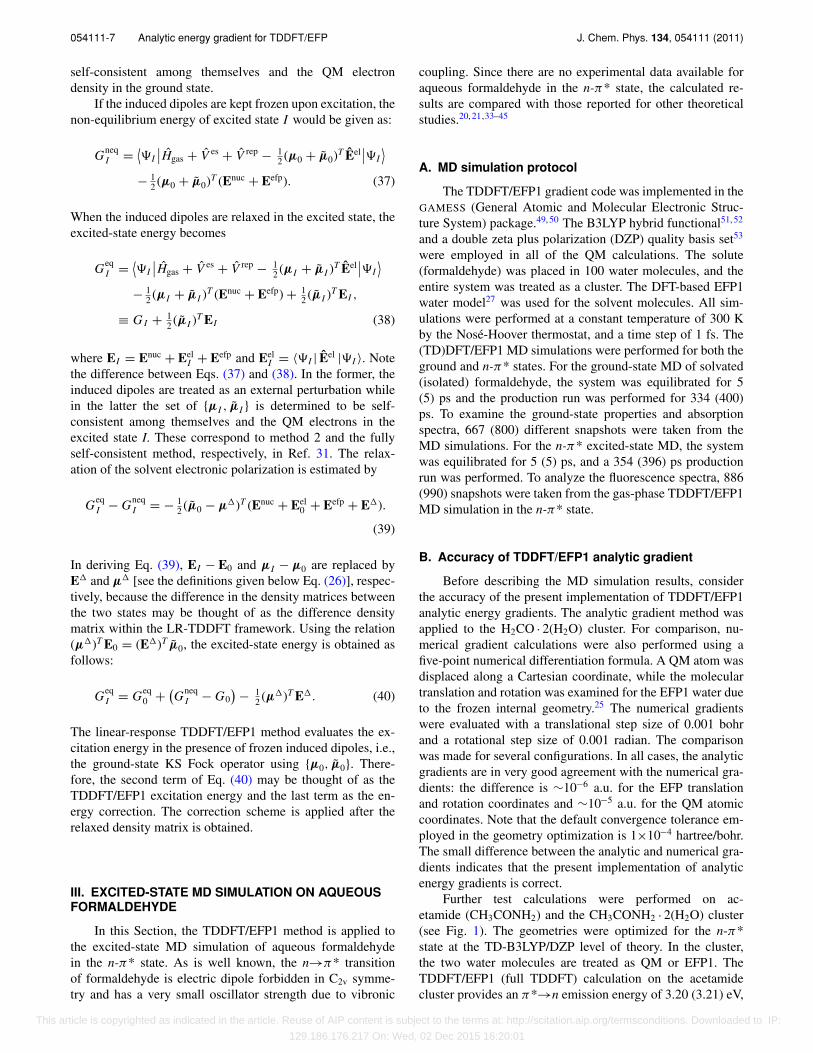
Further test calculations were performed on ac-etamide (CH3CONH2) and the CH3CONH2 · 2(H2O) cluster(see Fig. 1). The geometries were optimized for the n-π*state at the TD-B3LYP/DZP level of theory. In the cluster,the two water molecules are treated as QM or EFP1. TheTDDFT/EFP1 (full TDDFT) calculation on the acetamidecluster provides an π*→n emission energy of 3.20 (3.21) eV,

This article is copyrighted as indicated in the article. Reuse of AIP content is subject to the terms at: http://scitation.aip.org/termsconditions. Downloaded to IP:

129.186.176.217 On: Wed, 02 Dec 2015 16:20:01

054111-8 Minezawa et al. J. Chem. Phys. 134, 054111 (2011)

FIG. 1. A cluster formed by acetamide and two water molecules: carbon(cyan), oxygen (red), nitrogen (blue), and hydrogen (white) atoms.

which is slightly blue-shifted with respect to that of the iso-lated acetamide, 3.23 eV. Notably, the TDDFT/EFP1 valueis comparable to the full TDDFT estimate. Table I summa-rizes the n-π* state geometric parameters and vibrationalfrequencies of acetamide and the acetamide cluster. The vi-brational frequencies were obtained by the numerical dif-ferentiation of the analytic energy gradients, and no imagi-nary frequency was observed. The TDDFT/EFP1 results arein good agreement with those obtained by the full TDDFT.Therefore, the present implementation of TDDFT/EFP1 ana-lytic energy gradients is correct for both geometry optimiza-tions and force constant matrix calculations.

C. Absorption spectra of formaldehyde in gas phaseand in solution

Table II summarizes the average ground state geometricparameters of formaldehyde. The computed ground-state ge-ometry shows good agreement with experimental results.54 Toexamine the solvent effects on the solute electronic structure,the average geometric parameters are determined using thesnapshots taken from the simulations of isolated and solvatedformaldehyde. As clearly seen in the geometry and dipole mo-ment, the presence of water molecules significantly affects thesolute electronic structure, as embodied in the dipole moment,

TABLE I. Selected n-π* state geometric parameters and vibrational fre-quencies of acetamide (CH3CONH2) and the CH3CONH2 ·2H2O cluster.Bond lengths are in angstroms, angles in degrees, and vibrational frequen-cies in cm−1.

Acetamide Acetamide+two water Acetamide+two EFP1

Geometric parameters

r(CC) 1.512 1.511 1.511r(CO) 1.353 1.377 1.373r(CN) 1.421 1.400 1.402 CCO 113.4 112.0 112.3 NCO 112.4 112.1 112.1 CCN 116.9 118.5 118.2

Vibrational frequencies

CN stretch 1265 1314 1320CO stretch 1391 1354 1375

TABLE II. Average geometric parameters and dipole moments offormaldehyde in the ground and n-π* states obtained by the (TD)DFT(B3LYP/DZP) method. The standard deviations are given in parentheses.Bond lengths are in angstroms, angles in degrees, and dipole moments indebye.

Gas (0 K) Gas (300 K) Experimentala Solution (300 K)

Ground state

r(CO) 1.213 1.21 (0.02) 1.203 (0.003) 1.22 (0.02)r(CH) 1.111 1.12 (0.03) 1.099 (0.009) 1.10 (0.03) HCH′ 115.9 116 (4) 116.5 (1.2) 117 (4) HCO 122.1 122 (4) 121 (4) O-CHH′b 0.0 4 (3) 4 (3)Dipole 2.35 2.34 (0.09) 3.15 (0.26)

n-π* state

r(CO) 1.309 1.31 (0.02) 1.31 (0.03)r(CH) 1.098 1.10 (0.03) 1.10 (0.03) HCH′ 117.2 118 (6) 118 (6) HCO 116.4 117 (5) 116 (5) O-CHH′ 31.5 26 (12) 27 (12)Dipole 1.67 1.68 (0.07) 2.21 (0.21)

aExperimental estimation based on the infrared measurement (Ref. 54).bAveraging absolute values of out-of-plane angles.

but has very little effect on the geometric structure. The aver-age dipole moment is increased by 0.81 D with respect to thegas-phase average value of 2.34 D. In addition, the distribu-tion of dipole moments becomes much broader; the standarddeviation is increased by 0.17 D.

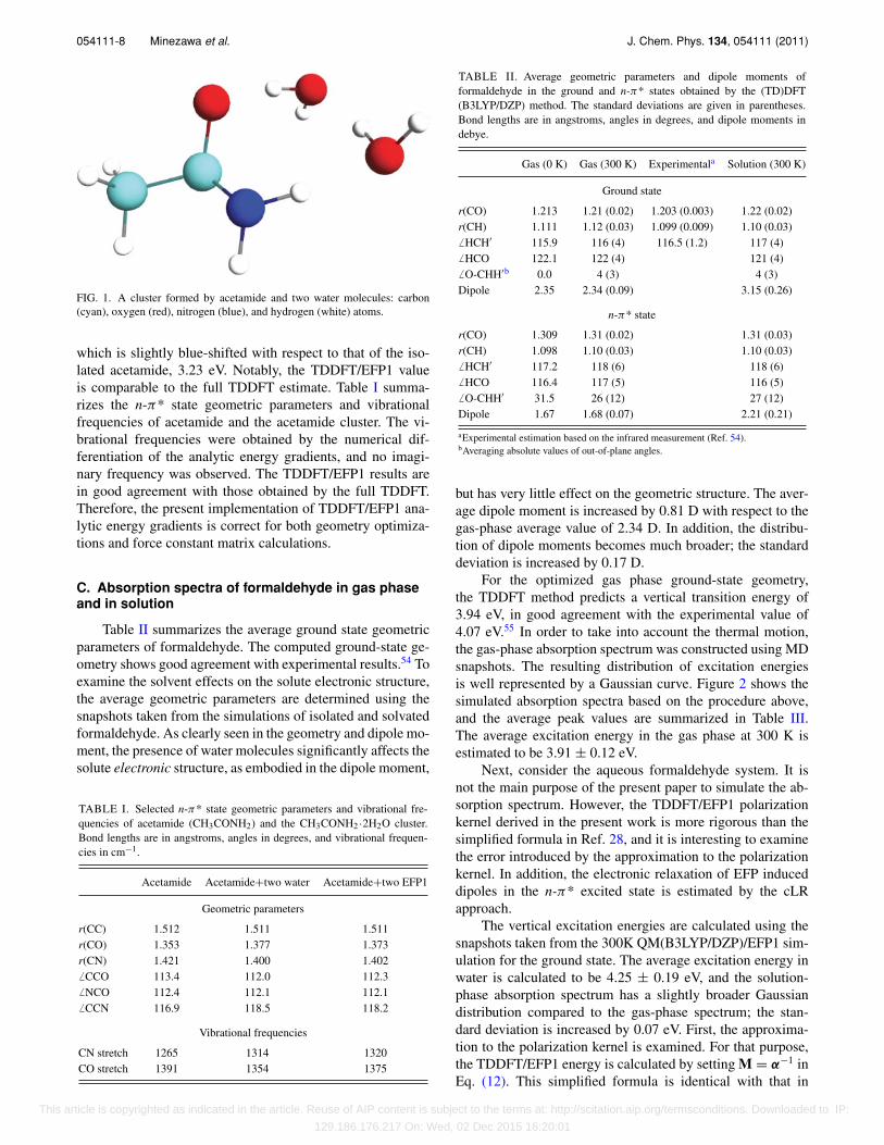
For the optimized gas phase ground-state geometry,the TDDFT method predicts a vertical transition energy of3.94 eV, in good agreement with the experimental value of4.07 eV.55 In order to take into account the thermal motion,the gas-phase absorption spectrum was constructed using MDsnapshots. The resulting distribution of excitation energiesis well represented by a Gaussian curve. Figure 2 shows thesimulated absorption spectra based on the procedure above,and the average peak values are summarized in Table III.The average excitation energy in the gas phase at 300 K isestimated to be 3.91 ± 0.12 eV.

Next, consider the aqueous formaldehyde system. It isnot the main purpose of the present paper to simulate the ab-sorption spectrum. However, the TDDFT/EFP1 polarizationkernel derived in the present work is more rigorous than thesimplified formula in Ref. 28, and it is interesting to examinethe error introduced by the approximation to the polarizationkernel. In addition, the electronic relaxation of EFP induceddipoles in the n-π* excited state is estimated by the cLRapproach.

The vertical excitation energies are calculated using thesnapshots taken from the 300K QM(B3LYP/DZP)/EFP1 sim-ulation for the ground state. The average excitation energy inwater is calculated to be 4.25 ± 0.19 eV, and the solution-phase absorption spectrum has a slightly broader Gaussiandistribution compared to the gas-phase spectrum; the stan-dard deviation is increased by 0.07 eV. First, the approxima-tion to the polarization kernel is examined. For that purpose,the TDDFT/EFP1 energy is calculated by setting M = α−1 inEq. (12). This simplified formula is identical with that in

This article is copyrighted as indicated in the article. Reuse of AIP content is subject to the terms at: http://scitation.aip.org/termsconditions. Downloaded to IP:

129.186.176.217 On: Wed, 02 Dec 2015 16:20:01

054111-9 Analytic energy gradient for TDDFT/EFP J. Chem. Phys. 134, 054111 (2011)

FIG. 2. TDDFT (B3LYP/DZP) simulated spectra for n→π* (red) andπ*→n (blue, shaded) vertical transition energies (eV) of formaldehyde inthe gas phase and in aqueous solution.

Ref. 28 and provides an excitation energy of 4.27 ± 0.18 eV,which is increased only by 0.02 eV with respect to that ob-tained by the present more rigorous TDDFT/EFP1 excitationenergy formula (4.25 ± 0.19 eV). The small energy differ-ence indicates a weak dependence of the excitation energyon the expression of polarization kernel. Yoo et al.28 havediscussed the direct and indirect contributions of EFP1 sol-vent molecules to the TDDFT excitation energy. The formercomes from the polarization kernel f pol in the coupling matrixgiven in Eq. (9) and the latter results from the other compo-nents in the coupling matrix such as orbital energies and theexchange-correlation kernel. The present results imply thatthe indirect component is the dominant factor in determin-ing the TDDFT/EFP1 excitation energies. Although the com-puted excitation energies are slightly different, the approxi-mation employed in Ref. 28 is very useful in that the simpli-fication can reduce the computational cost dramatically. TheTDDFT/EFP1 energy computation based on the present for-mula requires a number of iterations for each Davidson trialvector to obtain the self-consistent induced dipole moments

TABLE III. Average vertical transition energies (eV) of formaldehydein vacuum and aqueous solution obtained by the (TD)DFT (B3LYP/DZP)method. The standard deviations are given in parentheses.

Gas (0 K) Gas (300 K) Solution (300 K)

n→π* 3.94 3.91 (0.12) 4.25 (0.19) 4.24 (0.19)a

π*→n 2.96 3.00 (0.25) 3.03 (0.27) 3.02 (0.27)a

a Corrected linear response method, Eq. (40).

[see Eq. (14)]. In a serial run using a 2.66 GHz workstation,for example, it takes 31 (16) seconds to obtain the TDDFT ex-citation energy and the response density by the present (pre-vious approximate) method. Interestingly, the correspondinggas-phase computation requires 15 seconds.

Now, consider the cLR method applied to estimate therelaxation of the EFP induced dipoles. Table III shows theTDDFT/EFP1 excitation energies obtained with and withoutthe cLR approach. Evidently, the cLR method makes a negli-gible contribution (∼0.01 eV) to the excitation energies. Thismay be attributed to the use of the explicit EFP solvent model.The EFP1 water has permanent multipoles for describing theelectrostatic interaction. The excitation energy in solution re-flects not only the difference in the solvent electronic polar-ization between the ground and excited states, but also thatarising from the solute-solvent electrostatic interaction. In thefollowing discussion, the transition energies in the fourth col-umn in Table III are employed. The excitation energy differ-ence between the gas and solution phases, the solvatochromicshift, is calculated to be 0.34 eV, which is comparable to theexperimental value of 0.21 eV for acetone56 as well as to pre-vious theoretical results.20,34–42

D. Fluorescence spectra of formaldehyde in gasphase and in solution

The average geometrical parameters of formaldehyde inthe n-π* excited state are tabulated in Table II. Comparedwith the ground-state optimized structure, the most impor-tant change is the pyramidalization of the carbonyl group; theout-of-plane angle from the O=C bond to the CHH′ plane( O-CHH′) is about 30◦. The change in out-of-plane angle isdue to the electron migration from the oxygen lone pair to theπ* orbital, and the sp2 carbonyl carbon atom gains some ad-ditional p character. Furthermore, the C=O bond is stretchedby 0.1 Å and the HCO angle decreases by 5◦. The solventeffects hardly modify the n-π* state solute geometry; the dif-ference in geometric parameters between the gas and aqueoussolution is less than 0.01 Å and 1◦. Both in the gas and so-lution phases, the dipole moment is much smaller in the ex-cited state than in the ground state; the average dipole momentdecreases by 0.66 and 0.94 D for the isolated and solvatedformaldehyde, respectively.

The gas-phase fluorescence spectrum of formaldehyde iscalculated using the snapshots from the TDDFT MD simula-tion in the n-π* state at 300 K. The gas-phase average emis-sion energy is estimated to be 3.00 ± 0.25 eV, which gives aStokes shift (the difference between the absorption and emis-sion energies) of 0.91 eV. As shown in Fig. 2, the fluorescencespectrum deviates strongly from a Gaussian distribution. Toestimate the asymmetry of the distribution of excitation ener-gies and geometric parameters, skewness is introduced for thedistribution of variable x as follows,

Ndata∑i=1

(xi − x)3

Ndataσ 3x

, (41)

where, xi is the value of x for sample i and Ndata is thetotal number of data points. x and σx are the average and

This article is copyrighted as indicated in the article. Reuse of AIP content is subject to the terms at: http://scitation.aip.org/termsconditions. Downloaded to IP:

129.186.176.217 On: Wed, 02 Dec 2015 16:20:01

054111-10 Minezawa et al. J. Chem. Phys. 134, 054111 (2011)

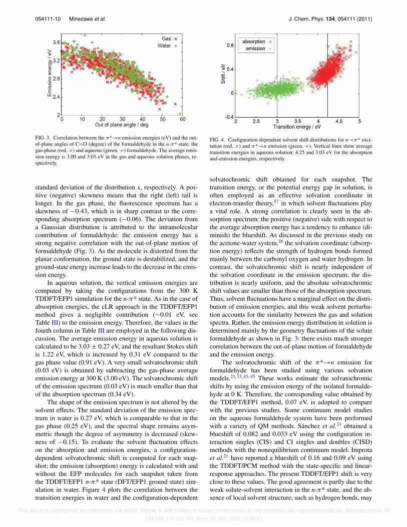
FIG. 3. Correlation between the π*→n emission energies (eV) and the out-of-plane angles of C=O (degree) of the formaldehyde in the n-π* state: thegas-phase (red, ×) and aqueous (green, +) formaldehyde. The average emis-sion energy is 3.00 and 3.03 eV in the gas and aqueous solution phases, re-spectively.

standard deviation of the distribution x, respectively. A pos-itive (negative) skewness means that the right (left) tail islonger. In the gas phase, the fluorescence spectrum has askewness of −0.43, which is in sharp contrast to the corre-sponding absorption spectrum (−0.06). The deviation froma Gaussian distribution is attributed to the intramolecularcontribution of formaldehyde: the emission energy has astrong negative correlation with the out-of-plane motion offormaldehyde (Fig. 3). As the molecule is distorted from theplanar conformation, the ground state is destabilized, and theground-state energy increase leads to the decrease in the emis-sion energy.

In aqueous solution, the vertical emission energies arecomputed by taking the configurations from the 300 KTDDFT/EFP1 simulation for the n-π* state. As in the case ofabsorption energies, the cLR approach in the TDDFT/EFP1method gives a negligible contribution (∼0.01 eV, seeTable III) to the emission energy. Therefore, the values in thefourth column in Table III are employed in the following dis-cussion. The average emission energy in aqueous solution iscalculated to be 3.03 ± 0.27 eV, and the resultant Stokes shiftis 1.22 eV, which is increased by 0.31 eV compared to thegas phase value (0.91 eV). A very small solvatochromic shift(0.03 eV) is obtained by subtracting the gas-phase averageemission energy at 300 K (3.00 eV). The solvatochromic shiftof the emission spectrum (0.03 eV) is much smaller than thatof the absorption spectrum (0.34 eV).

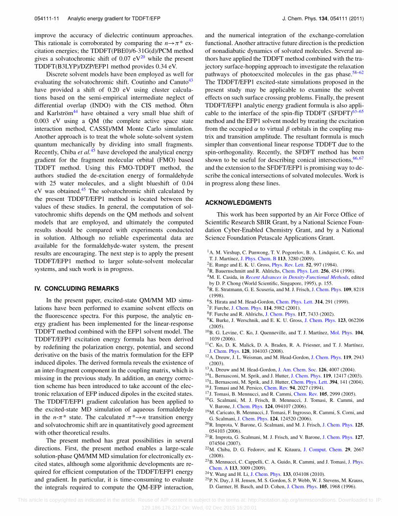
The shape of the emission spectrum is not altered by thesolvent effects. The standard deviation of the emission spec-trum in water is 0.27 eV, which is comparable to that in thegas phase (0.25 eV), and the spectral shape remains asym-metric though the degree of asymmetry is decreased (skew-ness of −0.15). To evaluate the solvent fluctuation effectson the absorption and emission energies, a configuration-dependent solvatochromic shift is computed for each snap-shot; the emission (absorption) energy is calculated with andwithout the EFP molecules for each snapshot taken fromthe TDDFT/EFP1 n-π* state (DFT/EFP1 ground state) sim-ulation in water. Figure 4 plots the correlation between thetransition energies in water and the configuration-dependent

FIG. 4. Configuration-dependent solvent shift distributions for n→π* exci-tation (red, ×) and π*→n emission (green, +). Vertical lines show averagetransition energies in aqueous solution: 4.25 and 3.03 eV for the absorptionand emission energies, respectively.

solvatochromic shift obtained for each snapshot. Thetransition energy, or the potential energy gap in solution, isoften employed as an effective solvation coordinate inelectron-transfer theory,57 in which solvent fluctuations playa vital role. A strong correlation is clearly seen in the ab-sorption spectrum: the positive (negative) side with respect tothe average absorption energy has a tendency to enhance (di-minish) the blueshift. As discussed in the previous study onthe acetone-water system,28 the solvation coordinate (absorp-tion energy) reflects the strength of hydrogen bonds formedmainly between the carbonyl oxygen and water hydrogen. Incontrast, the solvatochromic shift is nearly independent ofthe solvation coordinate in the emission spectrum; the dis-tribution is nearly uniform, and the absolute solvatochromicshift values are smaller than those of the absorption spectrum.Thus, solvent fluctuations have a marginal effect on the distri-bution of emission energies, and this weak solvent perturba-tion accounts for the similarity between the gas and solutionspectra. Rather, the emission energy distribution in solution isdetermined mainly by the geometry fluctuations of the soluteformaldehyde as shown in Fig. 3: there exists much strongercorrelation between the out-of-plane motion of formaldehydeand the emission energy.

The solvatochromic shift of the π*→n emission forformaldehyde has been studied using various solvationmodels.21, 33,43–45 These works estimate the solvatochromicshifts by using the emission energy of the isolated formalde-hyde at 0 K. Therefore, the corresponding value obtained bythe TDDFT/EFP1 method, 0.07 eV, is adopted to comparewith the previous studies. Some continuum model studieson the aqueous formaldehyde system have been performedwith a variety of QM methods. Sánchez et al.33 obtained ablueshift of 0.082 and 0.033 eV using the configuration in-teraction singles (CIS) and CI singles and doubles (CISD)methods with the nonequilibrium continuum model. Improtaet al.21 have reported a blueshift of 0.16 and 0.09 eV usingthe TDDFT/PCM method with the state-specific and linear-response approaches. The present TDDFT/EFP1 shift is veryclose to these values. The good agreement is partly due to theweak solute-solvent interaction in the n-π* state, and the ab-sence of local solvent structure, such as hydrogen bonds, may

This article is copyrighted as indicated in the article. Reuse of AIP content is subject to the terms at: http://scitation.aip.org/termsconditions. Downloaded to IP:

129.186.176.217 On: Wed, 02 Dec 2015 16:20:01

054111-11 Analytic energy gradient for TDDFT/EFP J. Chem. Phys. 134, 054111 (2011)

improve the accuracy of dielectric continuum approaches.This rationale is corroborated by comparing the n→π* ex-citation energies; the TDDFT(PBE0)/6-31G(d)/PCM methodgives a solvatochromic shift of 0.07 eV20 while the presentTDDFT(B3LYP)/DZP/EFP1 method provides 0.34 eV.

Discrete solvent models have been employed as well forevaluating the solvatochromic shift. Coutinho and Canuto43

have provided a shift of 0.20 eV using cluster calcula-tions based on the semi-empirical intermediate neglect ofdifferential overlap (INDO) with the CIS method. Öhrnand Karlström44 have obtained a very small blue shift of0.003 eV using a QM (the complete active space stateinteraction method, CASSI)/MM Monte Carlo simulation.Another approach is to treat the whole solute-solvent systemquantum mechanically by dividing into small fragments.Recently, Chiba et al.45 have developed the analytical energygradient for the fragment molecular orbital (FMO) basedTDDFT method. Using this FMO-TDDFT method, theauthors studied the de-excitation energy of formaldehydewith 25 water molecules, and a slight blueshift of 0.04eV was obtained.45 The solvatochromic shift calculated bythe present TDDFT/EFP1 method is located between thevalues of these studies. In general, the computation of sol-vatochromic shifts depends on the QM methods and solventmodels that are employed, and ultimately the computedresults should be compared with experiments conductedin solution. Although no reliable experimental data areavailable for the formaldehyde-water system, the presentresults are encouraging. The next step is to apply the presentTDDFT/EFP1 method to larger solute-solvent molecularsystems, and such work is in progress.

IV. CONCLUDING REMARKS

In the present paper, excited-state QM/MM MD simu-lations have been performed to examine solvent effects onthe fluorescence spectra. For this purpose, the analytic en-ergy gradient has been implemented for the linear-responseTDDFT method combined with the EFP1 solvent model. TheTDDFT/EFP1 excitation energy formula has been derivedby redefining the polarization energy, potential, and secondderivative on the basis of the matrix formulation for the EFPinduced dipoles. The derived formula reveals the existence ofan inter-fragment component in the coupling matrix, which ismissing in the previous study. In addition, an energy correc-tion scheme has been introduced to take account of the elec-tronic relaxation of EFP induced dipoles in the excited states.The TDDFT/EFP1 gradient calculation has been applied tothe excited-state MD simulation of aqueous formaldehydein the n-π* state. The calculated π*→n transition energyand solvatochromic shift are in quantitatively good agreementwith other theoretical results.

The present method has great possibilities in severaldirections. First, the present method enables a large-scalesolution-phase QM/MM MD simulation for electronically ex-cited states, although some algorithmic developments are re-quired for efficient computation of the TDDFT/EFP1 energyand gradient. In particular, it is time-consuming to evaluatethe integrals required to compute the QM-EFP interaction,

and the numerical integration of the exchange-correlationfunctional. Another attractive future direction is the predictionof nonadiabatic dynamics of solvated molecules. Several au-thors have applied the TDDFT method combined with the tra-jectory surface-hopping approach to investigate the relaxationpathways of photoexcited molecules in the gas phase.58–62

The TDDFT/EFP1 excited-state simulations proposed in thepresent study may be applicable to examine the solventeffects on such surface crossing problems. Finally, the presentTDDFT/EFP1 analytic energy gradient formula is also appli-cable to the interface of the spin-flip TDDFT (SFDFT)63–65

method and the EFP1 solvent model by treating the excitationfrom the occupied α to virtual β orbitals in the coupling ma-trix and transition amplitude. The resultant formula is muchsimpler than conventional linear response TDDFT due to thespin-orthogonality. Recently, the SFDFT method has beenshown to be useful for describing conical intersections,66, 67

and the extension to the SFDFT/EFP1 is promising way to de-scribe the conical intersections of solvated molecules. Work isin progress along these lines.

ACKNOWLEDGMENTS

This work has been supported by an Air Force Office ofScientific Research SBIR Grant, by a National Science Foun-dation Cyber-Enabled Chemistry Grant, and by a NationalScience Foundation Petascale Applications Grant.

1A. M. Virshup, C. Punwong, T. V. Pogorelov, B. A. Lindquist, C. Ko, andT. J. Martínez, J. Phys. Chem. B 113, 3280 (2009).

2E. Runge and E. K. U. Gross, Phys. Rev. Lett. 52, 997 (1984).3R. Bauernschmitt and R. Ahlrichs, Chem. Phys. Lett. 256, 454 (1996).4M. E. Casida, in Recent Advances in Density-Functional Methods, editedby D. P. Chong (World Scientific, Singapore, 1995), p. 155.

5R. E. Stratmann, G. E. Scuseria, and M. J. Frisch, J. Chem. Phys. 109, 8218(1998).

6S. Hirata and M. Head-Gordon, Chem. Phys. Lett. 314, 291 (1999).7F. Furche, J. Chem. Phys. 114, 5982 (2001).8F. Furche and R. Ahlrichs, J. Chem. Phys. 117, 7433 (2002).9K. Burke, J. Werschnik, and E. K. U. Gross, J. Chem. Phys. 123, 062206(2005).

10B. G. Levine, C. Ko, J. Quenneville, and T. J. Martínez, Mol. Phys. 104,1039 (2006).

11C. Ko, D. K. Malick, D. A. Braden, R. A. Friesner, and T. J. Martínez,J. Chem. Phys. 128, 104103 (2008).

12A. Dreuw, J. L. Weisman, and M. Head-Gordon, J. Chem. Phys. 119, 2943(2003).

13A. Dreuw and M. Head-Gordon, J. Am. Chem. Soc. 126, 4007 (2004).14L. Bernasconi, M. Sprik, and J. Hutter, J. Chem. Phys. 119, 12417 (2003).15L. Bernasconi, M. Sprik, and J. Hutter, Chem. Phys. Lett. 394, 141 (2004).16J. Tomasi and M. Persico, Chem. Rev. 94, 2027 (1994).17J. Tomasi, B. Mennucci, and R. Cammi, Chem. Rev. 105, 2999 (2005).18G. Scalmani, M. J. Frisch, B. Mennucci, J. Tomasi, R. Cammi, and

V. Barone, J. Chem. Phys. 124, 094107 (2006).19M. Caricato, B. Mennucci, J. Tomasi, F. Ingrosso, R. Cammi, S. Corni, and

G. Scalmani, J. Chem. Phys. 124, 124520 (2006).20R. Improta, V. Barone, G. Scalmani, and M. J. Frisch, J. Chem. Phys. 125,

054103 (2006).21R. Improta, G. Scalmani, M. J. Frisch, and V. Barone, J. Chem. Phys. 127,

074504 (2007).22M. Chiba, D. G. Fedorov, and K. Kitaura, J. Comput. Chem. 29, 2667

(2008).23B. Mennucci, C. Cappelli, C. A. Guido, R. Cammi, and J. Tomasi, J. Phys.

Chem. A 113, 3009 (2009).24Y. Wang and H. Li, J. Chem. Phys. 133, 034108 (2010).25P. N. Day, J. H. Jensen, M. S. Gordon, S. P. Webb, W. J. Stevens, M. Krauss,

D. Garmer, H. Basch, and D. Cohen, J. Chem. Phys. 105, 1968 (1996).

This article is copyrighted as indicated in the article. Reuse of AIP content is subject to the terms at: http://scitation.aip.org/termsconditions. Downloaded to IP:

129.186.176.217 On: Wed, 02 Dec 2015 16:20:01

054111-12 Minezawa et al. J. Chem. Phys. 134, 054111 (2011)

26M. S. Gordon, M. A. Freitag, P. Bandyopadhyay, J. H. Jensen, V. Kairys,and W. J. Stevens, J. Phys. Chem. A 105, 293 (2001).

27I. Adamovic, M. A. Freitag, and M. S. Gordon, J. Chem. Phys. 118, 6725(2003).

28S. Yoo, F. Zahariev, S. Sok, and M. S. Gordon, J. Chem. Phys. 129, 144112(2008).

29D. Si and H. Li, J. Chem. Phys. 133, 144112 (2010).30H. Li, H. M. Netzloff, and M. S. Gordon, J. Chem. Phys. 125, 194103

(2006).31P. Arora, L. V. Slipchenko, S. P. Webb, A. DeFusco, and M. S. Gordon,

J. Phys. Chem. A 114, 6742 (2010).32A. DeFusco, M. W. Schmidt, J. Ivanic, and M. S. Gordon (unpublished).33M. L. Sánchez, M. A. Aguilar, and F. J. Olivares del Valle, J. Phys. Chem.

99, 15758 (1995).34B. Mennucci, R. Cammi, and J. Tomasi, J. Chem. Phys. 109, 2798

(1998).35K. Naka, A. Morita, and S. Kato, J. Chem. Phys. 110, 3484 (1999).36M. E. Martín, M. L. Sánchez, F. J. Olivares del Valle, M. A. Aguilar,

J. Chem. Phys. 113, 6308 (2000).37Y. Kawashima, M. Dupuis, and K. Hirao, J. Chem. Phys. 117, 248 (2002).38J. Kongsted, A. Osted, K. V. Mikkelsen, P.-O. Åstrand, and O. Christiansen,

J. Chem. Phys. 121, 8435 (2004).39S. Hirata, M. Valiev, M. Dupuis, S. S. Xantheas, S. Sugiki, and H. Sekino,

Mol. Phys. 103, 2255 (2005).40A. Öhrn and G. Karlström, Mol. Phys. 104, 3087 (2006).41Z. R. Xu and S. Matsika, J. Phys. Chem. A 110, 12035 (2006).42Y. Mochizuki, Y. Komeiji, T. Ishikawa, T. Nakano, and H. Yamataka,

Chem. Phys. Lett. 437, 66 (2007).43K. Coutinho and S. Canuto, J. Chem. Phys. 113, 9132 (2000).44A. Öhrn and G. Karlström, J. Phys. Chem. A 110, 1934 (2006).45M. Chiba, D. G. Fedorov, T. Nagata, and K. Kitaura, Chem. Phys. Lett.

474, 227 (2009).46E. R. Davidson, J. Comput. Phys. 17, 87 (1975).47N. C. Handy and H. F. Schaefer, J. Chem. Phys. 81, 5031 (1984).48L. V. Slipchenko, J. Phys. Chem. A 114, 8824 (2010).

49M. W. Schmidt, K. K. Baldridge, J. A. Boatz, S. T. Elbert, M. S. Gordon,J. H. Jensen, S. Koseki, N. Matsunaga, K. A. Nguyen, S. J. Su, T. L. Win-dus, M. Dupuis, and J. A. Montgomery, Jr., J. Comput. Chem. 14, 1347(1993).

50M. S. Gordon and M. W. Schmidt, in Theory and Applications of Computa-tional Chemistry: The First Forty Years, edited by C. E. Dykstra, G. Frenk-ing, K. S. Kim, and G. E. Scuseria (Elsevier, Amsterdam, 2005), Chap. 41,pp. 1167–1189.

51A. D. Becke, J. Chem. Phys. 98, 5648 (1993).52C. Lee, W. Yang, and R. G. Parr, Phys. Rev. B 37, 785 (1988).53T. H. Dunning, Jr. and P. J. Hay, in Methods of Electronic Structure Theory,

edited by H. F. Schaefer (Plenum, New York, 1977), Chap. 1.54K. Yamada, T. Nakagawa, K. Kuchitsu, and Y. Morino, J. Mol. Spectrosc.

38, 70 (1971).55M. B. Robbin, Higher Excited States of Polyatomic Molecules, Vol. III

(Academic, New York, 1985).56N. S. Bayliss and E. G. McRae, J. Phys. Chem. 58, 1002 (1954).57For example, G. King and A. Warshel, J. Chem. Phys. 93, 8682 (1990).58C. F. Craig, W. R. Duncan, and O. V. Prezhdo, Phys. Rev. Lett. 95, 163001

(2005).59E. Tapavicza, I. Tavernelli, and U. Rothlisberger, Phys. Rev. Lett. 98,

023001 (2007).60E. Tapavicza, I. Tavernelli, U. Rothlisberger, C. Filippi, and M. E. Casida,

J. Chem. Phys. 129, 124108 (2008).61U. Werner, R. Mitric, T. Suzuki, and V. Bonacic-Koutecký, Chem. Phys.

349, 319 (2008).62R. Mitric, U. Werner, and V. Bonacic-Koutecký, J. Chem. Phys. 129,

164118 (2008).63Y. Shao, M. Head-Gordon, and A. I. Krylov, J. Chem. Phys. 118, 4807

(2003).64F. Wang and T. Ziegler, J. Chem. Phys. 121, 12191 (2004).65Z. Rinkevicius and H. Ågren, Chem. Phys. Lett. 491, 132 (2010).66N. Minezawa and M. S. Gordon, J. Phys. Chem. A 113, 12749 (2009).67M. Huix-Rotllant, B. Natarajan, A. Ipatov, C. M. Wawire, T. Deutsch, and

M. E. Casida, Phys. Chem. Chem. Phys. 12, 12811 (2010).

This article is copyrighted as indicated in the article. Reuse of AIP content is subject to the terms at: http://scitation.aip.org/termsconditions. Downloaded to IP:

129.186.176.217 On: Wed, 02 Dec 2015 16:20:01