Ocean Sci., 2, 223–236, 2006www.ocean-sci.net/2/223/2006/© Author(s) 2006. This work is licensedunder a Creative Commons License.

Ocean Science

Implementation of position assimilation for ARGO floats in arealistic Mediterranean Sea OPA model and twin experiment testing

V. Taillandier 1 and A. Griffa 1,2

1CNR-ISMAR, La Spezia, Italy2RSMAS, University of Miami, Florida, USA

Received: 23 February 2006 – Published in Ocean Sci. Discuss.: 18 Mai 2006Revised: 8 September 2006 – Accepted: 13 November 2006 – Published: 22 November 2006

Abstract. In this paper, a Lagrangian assimilation method ispresented and implemented in a realistic OPA OGCM withthe goal of providing an assessment of the assimilation ofrealistic Argo float position data. We focus on an applica-tion in the Mediterranean Sea, where in the framework ofthe MFSTEP project an array of Argo floats have been de-ployed with parking depth at 350 m and sampling interval of5 days. In order to quantitatively test the method, the “twinexperiment” approach is followed and synthetic trajectoriesare considered. The method is first tested using “perfect”data, i.e. without shear drift errors and with relatively highcoverage. Results show that the assimilation is effective, cor-recting the velocity field at the parking depth, as well as thevelocity profiles and the geostrophically adjusted mass field.We then consider the impact of realistic datasets, which arespatially sparse and characterized by shear drift errors. Suchdata provide a limited global correction of the model state,but they efficiently act on the location, intensity and shape ofthe described mesoscale structures of the intermediate circu-lation.

1 Introduction

Lagrangian measurements have experienced a dramatic in-crease in recent years. The Argo program, consisting of abroad-scale global array of floats, is now one of the maincomponents of the ocean observing system (http://www.argo.ucsd.edu). Argo floats are autonomous profiling floats thatspend most of their life freely drifting at a given parkingdepth, and that surface at a regular time interval measuringtemperature and salinity (TS) while ascending through thewater column. When at the surface, they communicate in-formation on position and TS profiles via satellite. Position

Correspondence to:V. Taillandier(vincent@sp.ismar.cnr.it)

data provide information on the ocean current at the parkingdepth, while TS data characterize the water masses.

Since Argo loats provide Near Real Time (NRT) infor-mation, they are well suited to be used in operational sys-tems for assimilation in Ocean General Circulation Mod-els (OGCM’s). Data on TS profiles are presently routinelyassimilated in many operational systems (http://www.argo.ucsd.edu/FrUseby Operational.html) while position dataare not included yet. On the other hand, float positionsrcontain information on an important model state variable,the Eulerian velocityu. The relationship betweenr anduis highly nonlinear, dr /dt = u(r , t), therefore the assimilationof r poses significant challenges. The first theoretical workson position assimilation (Ishikawa et al., 1996) simply cir-cumvented this problem using the quantity1r /1t, where1tis the interval between successive position information, as aproxy foru. This approximation holds for very small1t withrespect to the typical Lagrangian time scale TL (Molcard etal., 2003), which is of the order of 1–3 days at the surfaceand 5–10 days in the subsurface. In the case of Argo floats,since1t and TL are approximately of the same order, the ap-proximation is clearly violated and appropriate assimilationmethods that take into account the true nature of the obser-vations have to be considered.

In the last few years, growing attention has been givenand various methodologies proposed to assimilate positiondata. Different Lagrangian approaches have been investi-gated, going from Optimal Interpolation (OI) (Molcard et al.,2003, 2005;Ozgokmen et al., 2003), Kalman filtering (Ide etal., 2002; Kuznetsov et al., 2003), to variational techniques(Kamachi and O’ Brien, 1995; Nodet, 2006; Taillandier etal., 2006a). They have been tested mostly using simplifieddynamical systems, such as point vortices (Ide et al., 2002),or academic model configurations (Kamachi and O’Brien,1995; Molcard et al., 2005). Even though the results arevery encouraging and show the high potential of assimilat-ing Lagrangian data, there are still a number of issues to be

Published by Copernicus GmbH on behalf of the European Geosciences Union.

224 V. Taillandier and A. Griffa: Implementation of ARGO position assimilation

addressed regarding the actual application to Argo data as-similation in operational OGCM.

The first challenge to be addressed is the implementationof these assimilation methods in realistic circulation models.In particular, with respect to previous applications in ideal-ized model configurations with a reduced number of isopy-cnal layers (Molcard et al., 2005), expected improvementsshould include complex geometry and topography, continu-ous stratification and TS mass variables in the model state.Other challenges are inherent to the nature and distributionof the Argo datasets. NRT position information is obtainedwhen the floats reach the ocean surface and communicate viasatellite. Such surface position data provide information onthe subsurface drift (at the parking depth) contaminated by“shear errors” due to additional drifts experienced during as-cent and descent motions (Park et al., 2005). The impactof such errors needs to be evaluated and possible techniquesto account for it should be investigated. Also, Argo floatpositions are provided at intervals1t of the order (or evengreater) than TL, so that successiver along observed trajec-tories might be weakly correlated. Therefore the informationcontent in terms of velocity might be degraded (Molcard etal., 2003). Finally, the realistic coverage of Argo floats in agiven region of the world ocean is expected to be quite low toresolve the mesoscale features of the circulation. These dif-ferent aspects have to be tested in order to verify the impactand potential of Argo position data if included in operationalobserving systems.

In this paper we present a Lagrangian assimilation methodfor realistic OGCM’s. The various points indicated above aretested with the goal of providing a complete assessment ofthe assimilation of realistic Argo floats. The inverse methodbuilds on previous works (Molcard et al., 2003, 2005; Tail-landier et al., 2006a) and conceptually follows the same threemain steps as in Molcard et al. (2005). First the position datar are used to correct the velocity fieldu at the parking depthzp using the variational method developed in Taillandier etal. (2006a). Then the velocity correction is projected over thewater column using statistical correlations while maintainingmass conservation. And finally the TS mass field is correctedin geostrophic balance with the correctedu profiles using avariational approach (Talangrand and Courtier, 1987), basedon the thermal wind and on the equation of state.

Here we consider a specific application to a realistic OPAmodel of the Mediterranean Sea. In the framework of theMFSTEP project (Pinardi et al., 2003;http://www.bo.ingv.it/mfstep/), a component of the world wide Argo project hasbeen carried out in the Mediterranean Sea. A total of morethan 20 floats have been deployed in the basin, characterizedby a time interval1t of approximately 5 days and by a park-ing depth zp of 350 m (Poulain, 2005). In order to test theperformances of the assimilation method in the “twin exper-iment” approach, synthetic floats with characteristics similarto the in-situ ones are released in a numerical circulation tobe identified. The sensitivity of the Lagrangian analysis to

shear errors and low coverage is considered in a second time.The paper is organized as follows. The method is pre-

sented in Sect. 2, while the set up for the numerical exper-iments is given in Sect. 3. The experiment results are pre-sented in Sect. 4. Assimilation skills with realistic Argo typedata are investigated in Sect. 5. Summary and discussion areprovided in Sect. 6.

2 Methodological aspects

The analysed (estimated) circulation is obtained from floatposition information by correcting a prior (background) cir-culation in a sequential way. Such model state correction isprovided every five days according to the cycling design ofthe Argo floats. Estimations of the velocity fieldu and of thecorresponding mass field (T, S) are detailed in the followingsections 2.1 and 2.2 respectively for each 5 day sequence,while the practical implementation of the method is summa-rized in Sect. 2.3.

2.1 Estimation of the model velocity field

The velocity field at the parking depth zp is estimated fromArgo data using the variational method developed by Tail-landier et al. (2006a). The method provides a bi-dimensionalvelocity increment1u(zp) for each 5 day sequence separat-ing two successive Argo float positions. In this approach,u(zp) is estimated minimizing a cost function which mea-sures the distance between the observed float position at theend of the sequence and the position of a prior trajectoryadvected in the background velocity field.1u(zp) is there-fore a time-independent correction (for the given sequence)of u(zp) mapped around the prior trajectory. Note that sheardrifts occurring on vertical float motions can be taken intoaccount in the computation of the prior trajectory but onlyu(zp) is estimated.

This variational method has been tested in Taillandier etal. (2006a), considering its performance by varying numberof floats P and time sampling1t. The results are positive,showing that the approach is effective and robust. Moreover,the method provides significant advantages with respect tothe previous works of Molcard et al. (2003, 2005), since itexpands the velocity correction all along trajectories and usesan appropriate covariance matrix. We notice that in Tail-landier et al. (2006a) an important issue was discussed forthe case of1t of the order or bigger than TL. This is of po-tential interest here given that TL is expected to be approxi-mately of the same order as1t (i.e. five days). It is pointedout that when strong vortices are sampled by various floats, itcan happen that successive positions “cross” each other be-cause the vortex curvature is not resolved by the trajectorysampling. Such coherent structures are therefore not cor-rectly estimated, since the obtained flow converges towardthe crossing points. This problem, which is inherent to the

Ocean Sci., 2, 223–236, 2006 www.ocean-sci.net/2/223/2006/

V. Taillandier and A. Griffa: Implementation of ARGO position assimilation 225

data, was illustrated in the case where the velocity field isreconstructed using data only, i.e. without prior circulation.In the experiments considered here, we expect that the use ofprior model circulations, and consequently the use of addi-tional information on the curvature, will help preventing thisphenomenon. We will come back on this issue discussing thenumerical results in Sect. 4.

In first approximation for regional and oceanic circula-tion scales, horizontal and vertical correlations of the motioncan be separated using linear regression profiles (Oschliesand Willebrand, 1996). Note that horizontal velocity cor-relations are specified by the length of mesoscale structuresdescribed by the float trajectories (Taillandier et al., 2006a).As discussed in Molcard et al. (2005), the velocity increment1u(zp) obtained from float positions at zp can be projectedon the water column as

1u(z)=R(z).1u(zp), z ∈ [0, h] (1)

where h is the depth of the basin andR represents the verti-cal projection operator.R(z) is computed from seasonal andspatial averages (in quasi-homogeneous regions) of the lin-ear regression coefficients linking each velocity componentat depth z with velocity at zp.

This projection of1u(zp) is funded on statistical means,without any constraint on model consistency. In order to in-troduce some dynamical constraints, we do enforce the as-sumption of basin volume conservation expressed by a non-divergent barotropic flow in the rigid lid formulation. To dothat, the depth integrated velocity increment is first expressedfrom Eq. (1) as

1U = 1u(zp).

∫[0,h]

R(z).dz (2)

Then its divergent part is removed while1U is further re-computed from the diagnostic of its stream function. Af-ter that, the updated barotropic flow increment1U, now inmodel consistency, is used to redefine the velocity incrementas

1u(z) = R(z).[

∫[0,h]

R(z).dz]−1.1U, z ∈ [0, h] (3)

This normalisation to the flat bottom case aims at modifyingthe amplitude of the velocity profile. It has been preferred toshifting the velocity profile. Notice that the two approachesare possible since the separation of single subsurface veloc-ity information into barotropic and baroclinic contributionsis underdetermined. The present approach allows to smoothhorizontal discrepancies on shallow zones, especially alongthe land-sea interface at the parking depth, with a consistentvelocity correction at the sea bottom.

2.2 Estimation of a dynamically consistent mass field

For mesoscale open sea applications like the present one,the isopycnal slopes can be adjusted, at least in first ap-proximation, to the velocity increment1u (expressed in

Eq. 3) in agreement with the thermal wind equation (Os-chlies and Willebrand, 1996). The corresponding TS correc-tion is searched on the sequence average since1u is time-independent. So the mass field estimation is provided by theresolution of a static inverse problem formulated in the fol-lowing variational approach.

Considering a prior model state (u, T, S), a variationδu ofthe velocity field infers a variation of its vertical shearδσ ,defined as∂zδu. This vertical structure is maintained by adensity variationδρ n geostrophic equilibrium as

δσ = −g/ρof.k×∇δρ (4)

where g is the gravity,ρo the density of reference,f the Cori-olis parameter,k the upward unit vector and∇ the horizontalgradient. The density variationδρ is linearly expressed withrespect to the equation of state. In case of a best-fit poly-nomial formulation (e.g. the one of Jackett and McDougall,1995), the first order perturbation of density around its priorvalueρ =

∑i,j αij .Ti .Sj is taken from

δρ =

∑i,j

αij .Ti−1.Sj−1.(i.S.δT + j.T .δS) (5)

whereδT and δS are the respective variations on the priortemperature and salinity profiles. Notice that this perturba-tion equation can be obtained from a local linearization (formodel values of T and S) of the equation of state used by theOGCM.

Here, we require that the shear variation1σ = ∂z 1uprovided by the analysis of the float positions (Eq. (3)) isfitted to the geostrophic velocity shear variation defined byEq. (4). This latter can be expressed using Eqs. (4–5) byδσ = M .(δT, δS), whereM is a linear model. The inverseproblem consists in finding the best combination (δT, δS), inthe neighbourhood of prior TS profiles, that minimises thecost function

J = (1σ − M .(δT , δS))T .(1σ − M .(δT , δS)) (6)

where T is the vector transpose. In numerical practice, Jis minimised using the steepest descent algorithm M1QN3(Gilbert and Lemarechal, 1989), in the direction of the gra-dient

∇J = −B.MT .(1σ − M .(δT , δS)) (7)

where the linear modelMT is governed by the adjoint equa-tions of Eqs. (4–5), andB is classically defined by back-ground error covariances. For the construction ofB, cross-covariances between temperature and salinity are not consid-ered as the balance on these two variables is explicitly con-strained by the equation of state (Eq. (5)). So only the uni-variate components are required and described by the fieldvariance. Notice that they intrinsically define the verticalweighting for the contribution of the velocity shear fitting. Innumerical practice, seasonal and space averages of the stan-dard deviation profiles for TS define the diagonal matrixB.

www.ocean-sci.net/2/223/2006/ Ocean Sci., 2, 223–236, 2006

226 V. Taillandier and A. Griffa: Implementation of ARGO position assimilation

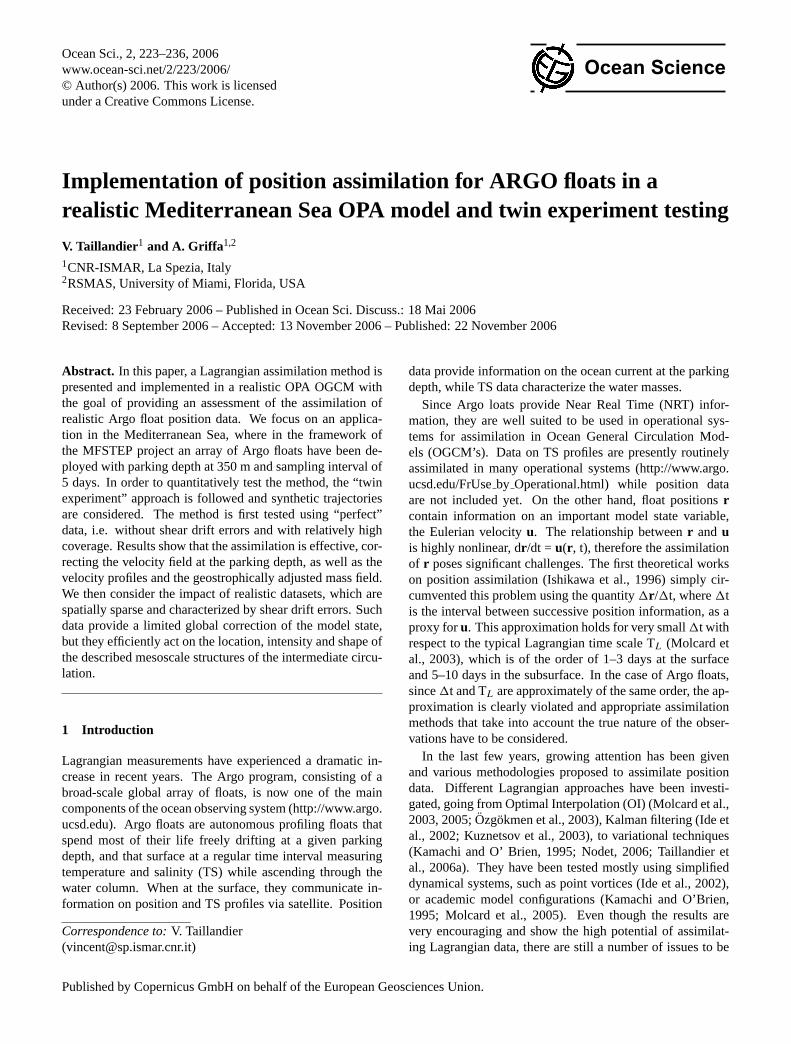
Fig. 1. Correlation and regression profiles of velocity componentsbetween depths z and zp=350 m.

2.3 Assimilation procedures

Estimates of the prior circulation for each 5 day sequencehave been implemented in two different assimilation proce-dures, referred to as “state of art” and “operational” respec-tively. Notice that each sequence initialization is stable sincethe corrected fields belong to the admissible model solutions.Both procedures have been tested in the twin experimentspresented in the following.

In the procedure “state of art”, variations of Argo float po-sitions during each cycle/sequence are used to estimate thevelocity and mass fields at the initial time of the assimila-tion sequence. The model is then run forward again for theconsidered sequence using the corrected initial conditions,so that prior model state and trajectories are updated withrespect to the initial state estimate. This procedure is char-acterised by a high computational cost as the CPU time of aforward model run is doubled, in addition to the estimationof the velocity and mass corrections. Note that CPU time re-quirements for a model state analysis is very small comparedto a forward run.

In the procedure “operational”, variations of float positionsduring each cycle/sequence are used to estimate the velocityand mass fields at the final time of the assimilation sequence.Prior model state computed on the sequence determines themodel update on the next sequence, and the prior float tra-jectories are not updated. This procedure is characterised byan equivalent computational cost as for a single forward run,always in addition to velocity and mass estimation.

3 Experimental set up

3.1 Modelling the Mediterranean circulation

The numerical model used here is an extended version of theprimitive equation model OPA with rigid lid (Madec et al.,1998), configured in the Mediterranean Sea. For the develop-ment and testing of the assimilation procedure, which is com-putationally demanding, a horizontal resolution at 1/8 degreehas been considered, while the statistical prior informationon R andB have been computed using a more refined reso-lution at 1/16 degree. For both configurations a vertical dis-cretization with 43 geopotential levels is considered. Themodel is initialised from rest by climatological hydrologicalconditions from MEDATLAS. It is forced by daily winds andheat fluxes from the ECMWF atmospheric forcing fields dur-ing the period 1987–2004. The spin-up has been performedrepeating the cycle three times. Characteristics of the gen-eral circulation and of the transports at several straits are ingood agreement with recent estimates from in-situ observa-tions (Beranger et al., 2005).

We concentrate on a case study in the North WesternMediterranean Sea, during the winter season. This region hasbeen chosen since it is a complex and interesting area with avigorous mesoscale field even at 350 m. Moreover, a goodcoverage of in-situ Argo floats has been maintained in thisregion during the MFSTEP project (see the 4 float trajecto-ries onhttp://poseidon.ogs.trieste.it/WP4/product.html). Asa first step, the statistical quantities have been computed frommodel outputs during 2000–2004. Horizontal motion scales,already described in Taillandier et al. (2006a) are character-ized by typical mesoscale length scales of the order of 20–30 km, and associated Eulerian time scales of the order of20–30 days. Vertical correlations are computed from the ve-locity fields to defineR (Eq. (1)), and from the active tracerfields TS to defineB (Eq. (7)). These correlations are com-puted independently for each velocity or tracer component,and averaged over the north western basin, to get wintermean representative profiles. As underlined in Sect. 2.2, onlythe variance profiles for tracer fields are involved in the con-struction ofB. In the region of interest, maximum variancefor temperature reaches 0.50◦C in the first 100 m, followedby a quick decrease to 0.15◦C in the intermediate layer. Forsalinity, the decrease from the maximum value of 0.12 PSUat surface is quasi linear, to reach 0.05 PSU at the parkingdepth.

Regression and correlation profiles for velocity are repre-sented in Fig. 1. They are very similar for the zonal andmeridional components. The velocity variations on the inter-mediate layer, between 150 m and 750 m, appear well corre-lated with velocity variations at the parking depth. Insteadin the surface layer and in the deep layer, correlation valuesdrop under 0.8. The linear regression coefficients decreasefrom 2.5 at sea surface until 0.4 at sea bottom. The profilecan be described by four straight lines: a surface segment

Ocean Sci., 2, 223–236, 2006 www.ocean-sci.net/2/223/2006/

V. Taillandier and A. Griffa: Implementation of ARGO position assimilation 227

between 0 m and 200 m associated to a sharp slope, an in-termediate segment extending to 600 m, a deep segment ex-tending to 1000 m associated to a slight slope, and a bottomsegment after 1000 m without slope. Considering Eq. (1), thefirst order derivative of the regression profile is related to therelative intensity of the vertical shear variations. As a con-sequence, the correction of the baroclinic velocity (Sect. 2.2)will be limited to the first 1000 m, and it is expected to becharacterized by decreasing amplitude from the sea surface,as in three distinct layers quite well correlated.

3.2 Numerical experiments

The sensitivity and robustness of the assimilating system hasbeen tested with a total of seventeen simulation experiments.A first set of experiments (Sect. 4) is directly finalized at test-ing the methodology and the two different implementationsof Sect. 2.3. It considers “ideal” data, i.e. data without obser-vational errors and with significant spatial coverage. On theother hand, a second set of experiments (Sect. 5) is aimed atinvestigating the performance in realistic conditions, i.e. withreduced coverage, for Argo float applications. Moreover, sur-face position data are used instead of positions at the parkingdepth. In this case, observational information is contami-nated by shear errors related to additional drifts experiencedduring ascent and descent motions. Notice that real in-situArgo floats have another source of observational error dueto the surface drift experienced before (after) the first (last)satellite fix. In this study, the surface drift error is not consid-ered for simplicity, since it depends on the specific details ofArgo communication. Our observational errors should thenbe considered as lower bounds with respect to in-situ errors.The numerical protocol of experimentation follows the clas-sical twin experiment approach, and can be summarized asfollows. Three different simulations are performed for eachexperiment using the circulation model (Sect. 3.1), all withthe same forcing functions corresponding to the month ofMarch 1999. The first run is correctly initialized from themodel state corresponding to March 1 1999, and it representsthe “truth” circulationutru. Synthetic floats are launched inthe truth run and advected by the numerical velocity field.The second run is initialized from a “wrong” initial condi-tion, corresponding to the model state of 1 March 2000, torepresent our incomplete knowledge of the true state of theocean. The position data extracted from the truth circulationare assimilated in this run, providing the “estimated” fielduest. Finally, the third run provides a “background” circula-tion ubck initialized with the same wrong initial condition asthe assimilation run, but without data assimilation. It pro-vides a reference simulation, where the circulation of March1999 evolves freely from the wrong initial conditions. Thesuccess of the assimilation is quantified in terms of conver-gence ofuest toward utru. In other words a successful as-similation is expected to correct the wrong initial conditions,driving the ocean state toward the truth.

Fig. 2. Details of a simulated Argo type trajectory. The high resolu-tion trajectory is shown, with superimposed the trajectory sampledat1t=5 days, as observed at the surface. Crosses indicate positionswhere the simulated float reaches or leaves its parking depth.

The numerical trajectories are computed following thesame cycle as in-situ Argo floats, using a fourth order Runge-Kutta scheme for advection. The cumulated duration of ver-tical motion is fixed to half a day, while the residence timein subsurface is equal to 4.5 days. In our numerical experi-ments two sets of data have been extracted from the numeri-cal trajectories: the “perfect data”, containing initial and finalpositions of each subsurface drift, that are utilized in the ide-alized experiments (Sect. 4), and the surface data, that takeinto account the shear drift and that are used in the realisticexperiments (Sect. 5). For in-situ floats, only surface posi-tions are available, provided in near-real time via satellite. InFig. 2, an example of the difference between the “perfect”data (marked by crosses) and “realistic” data observed at thesurface is shown along a single numerical trajectory. A totalof 182 simulated Argo floats have been advected in the truthcirculation during six cycles (Fig. 3). In the assimilation ex-periments, the influence of data coverage is studied varyingthe number of Argo type trajectories P equal to 182, 42, 9,4, 3 extracted from the original set. For all the cases, sim-ulated floats are released on the basin according to homoge-neous spatial distributions. This disables possible strategiesof float deployment to a priori improve observational infor-mation (e.g. Toner et al., 2001; Molcard et al., 2006). Asshown in Fig. 3, the Lagrangian description of the circulationshows an intense boundary current (the so-called NorthernCurrent) characterized by meanders and recirculation cells.Given the long Eulerian time scale (20–30 days), the trajec-tories are indicative of mesoscale structures, but they quicklytend to get sparse when P decreases. On the other hand, thedifference between “perfect” and “realistic” data, shown in

www.ocean-sci.net/2/223/2006/ Ocean Sci., 2, 223–236, 2006

228 V. Taillandier and A. Griffa: Implementation of ARGO position assimilation

Fig. 3. Lagrangian description of the truth circulationutru duringthe month of March 1999. Three coverages with different numberof trajectories P are represented: P=182 (c), P=42 (b), P=9 (c). Thelocations of float deployment are indicated by a cross. The compu-tational domain is bounded inside the box.

Fig. 2 has been assessed quantitatively. The ratio betweenthe mean shear drift and the mean drift at the parking depthreaches 19% considering the 182 simulated trajectories.

The assimilation system is quantitatively assessed using ameasure of the adjustment ofuest to utru. It is expressed bythe non dimensional quantity

E(z, t)=||utru(z, t)−uest(z, t)||2/||utru(z, t)−ubck(z, t)||2(8)

where|| u ||2=uT .u. The normalization term in denomina-

tor is used to reduce the dependency of the results from thespecific realization, i.e. from the time evolution of the back-ground simulation. This measure is integrated over the com-putational region shown in Fig. 3. It can be applied at a givendepth z or at a given sequence t. Notice that the time reso-lution is given by the duration of the sequence, so E valuesinvolve sequence averages foru.

4 Results of experiments with ideal data

The methodology (Sect. 2) is tested using perfect data(i.e. without shear error) and considering the effects of de-creasing coverage in a range of relatively high number offloats P equal to 182, 42, 9. The two different proceduresdiscussed in Sect. 2.3 are compared. The results are assessedfirst in terms of velocity estimation at the parking depth andthen in terms of velocity and mass estimation over the wholewater column.

4.1 Velocity estimation at the parking depth

The first assessment focuses on the analysis of the circulationat the parking depth zp. Results for P equal to 182, 42, 9 areshown in Fig. 4 in terms of time evolution of the adjustmenterror E(t) (defined in Eq. 8) during the one month assimila-tion period using the two procedures. For both of them, theadjustment of the velocity field at 350 m is increasingly bet-ter with data coverage, as expected. The mean slope of theerror decrease varies from 20% with low coverage (P equalto 9) to 35% with high coverage (P equal to 182). Whenconsidering the sequence by sequence evolution of E(t), itappears that the major adjustment occurs during the first twoanalyses. After that, E(t) continues to decrease in average,but oscillations can occur especially for P equal to 42 and9, with slight increases followed by marked decreases. Thiscan be explained considering the following points of view.In a fix point approximation (in which information locationsdo not change), the time scale characterising the assimilationadjustment is expected to coincide with the time scales of thecirculation structures, i.e. with the time over which the infor-mation is correlated. With high coverage (P equal to 182), thefix point approximation can be assumed, and the obtained ad-justment appears characterised by a constant decrease at theEulerian time scale (∼20 days). With low coverage instead,and given the relatively long Eulerian time scales, the veloc-ity field can be assumed time-independent with respect to the

Ocean Sci., 2, 223–236, 2006 www.ocean-sci.net/2/223/2006/

V. Taillandier and A. Griffa: Implementation of ARGO position assimilation 229

scale of motion of the floats. In this frozen field approxima-tion, local and fast adjustments to the truth circulation areprovided at the information location and at the Lagrangiantime scale (order of 3–5 days). Successive adjustments areexpected to occur when the floats enter and sample new cir-culation structures, providing new information. This appearto be the case for P equal to 9 or 42, where the decrease ofE(t) is characterised by secondary gaps due to the renewal ofdata information.

A comparison of the two assimilation procedures can nowbe performed. In the procedure “operational” (Fig. 4b), themodel state correction is operated at the end of each sequence(Sect. 2.3), so that the effect of the model state correction forsequence (t) appears at sequence (t+1). So this procedureonly benefits of five analyses during the assimilation period,instead of six as for the procedure “state of art” (Fig. 4a).In terms of adjustment, the evolution of E(t) appears similarin both procedures but translated of one sequence. So theadjustments E obtained at the final time with the procedure“operational”, 70% for P equal to 9, 40% for P equal to 42,20% for P equal to 182, are approximately the same as theones obtained a sequence before with the procedure “state ofart”.

An example of qualitative comparison between estimatedand truth circulations at the parking depth is drawn for therepresentative data coverage of P equal to 42 in Fig. 5. These5 day-averaged circulations are mapped during the last se-quence of the assimilation period. The results are similarfor the two procedures, even though slight differences stillremain on intensity and shape between the two estimated cir-culations. In both cases the assimilation appears to efficientlycorrect the field, and the estimates tend to converge towardthe truth field. The Northern Current confined along the coastin the background circulation appears wider in the estimatedcirculations. Its meanders and recirculation features presentin the truth circulation appear well estimated. Both intenseand weak mesoscale structures are replaced from their back-ground location with respect to the truth circulation.

We notice that in all the performed experiments, there isno evidence of problems in the velocity estimation when1t≥ TL as discussed in Taillandier et al. (2006a) (and men-tioned in Sect. 2.1) did not emerge. No unrealistic conver-gence in the estimated velocity field has been found. Thismight be partially due to the fact that the case in Taillandieret al. (2006a) was extreme in terms of intense sampling ofthe core of a very energetic vortex, even though also in thepresent experiments strong recirculation features and vor-tices are present and sampled at various rates, as shown inFig. 3. More conceptually, we think that the main reasonfor the difference is that in Taillandier et al. (2006a), the ve-locity field was reconstructed based on the float data only,while in the present experiments the data are assimilated ina model. The model provides a priori information on the ve-locity structure, so that the information on the curvature canbe corrected avoiding the emergence of unrealistic velocity

Fig. 4. Evolution of the adjustment error E(t) (in %) at the parkingdepth computed from perfect data with three coverages P=182, 42,9, using the assimilation procedure “state of art”(a) and “opera-tional”(b).

convergence and a correct estimate can be obtained.

4.2 Velocity estimation on the water column and impact ofTS correction

The effect of the velocity estimation at the parking depthis now investigated on the other layers. The quality of themodel state analyses from float positions depends on the ve-locity adjustment at depth, which is given directly by theshape of linear regression profiles (see Eq. (1)) and indi-rectly by the mass field adjustment. This latter mechanismcan either be forced through the estimation of temperatureand salinity (Sect. 2.2), or lead by a natural adjustment ofthe mass field onto the estimated velocity field. In order to

www.ocean-sci.net/2/223/2006/ Ocean Sci., 2, 223–236, 2006

230 V. Taillandier and A. Griffa: Implementation of ARGO position assimilation

Fig. 5. Velocity fields at the parking depth at the end of the assimilation period. The background circulation is represented in panel(a),the truth circulation in panel(b), and the estimated circulation with the procedure “state of art” (“operational”) in panels(c) (d) using 42trajectories. The hydrologic section is drawn as a straight line.

evaluate the impact of TS estimation, both approaches aretested when assimilating the three data sets P equal to 182,42, 9. The corresponding adjustment errors E(z) (given inEq. (8) at the end of the assimilation period) are representedin Fig. 6. It appears that the profiles E(z) are improved whenobtained with TS estimation. This is particularly the casewhen the procedure “operational” is used. On the other hand,there is only a slight improvement when the procedure “stateof art” is used. So the relaxation of the mass field is effec-tively operated during the sequence reanalysis, i.e. while it isset to the velocity estimate on the same sequence (Sect. 2.3).These adjustment errors appear to decrease from the sea sur-face to a minimum value close to the parking depth, increas-ing then with depth. This is particularly accentuated withhigh data coverage (P equal to 182), while the adjustmentstend to be homogeneous on the water column with low datacoverage (P equal to 9). This general feature can be ex-plained considering the velocity correlations (Fig. 1) impli-

cated in the vertical velocity projection (Eq. 1). As describedin Sect. 3.1, the amplitudes of the velocity variations at thesea surface are at least twice than those in the intermedi-ate layer, while surface and intermediate currents are weaklycorrelated. So adjustment errors obviously increase in thesurface layer. On the other hand, E(z) values on the deeplayer are mainly governed by the barotropic flow adjustmentin which the baroclinic structure of the model state analysesis involved. So the quality of velocity estimates in the deeplayer is degraded because of the estimation of the baroclinicstructure, through the specification of vertical velocity shear,which is poor at depth (Sect. 3.1). Moreover, this degrada-tion of E(z) in the deep layers is accentuated when the adjust-ment of the model mass field is not effective. As shown forthe “operational” procedure (Fig. 6 left panels), adjustmenterrors of deep currents are increased in absence of mass fieldestimation. A quantitative comparison of the effectiveness ofthe two assimilation procedures versus z can be performed

Ocean Sci., 2, 223–236, 2006 www.ocean-sci.net/2/223/2006/

V. Taillandier and A. Griffa: Implementation of ARGO position assimilation 231

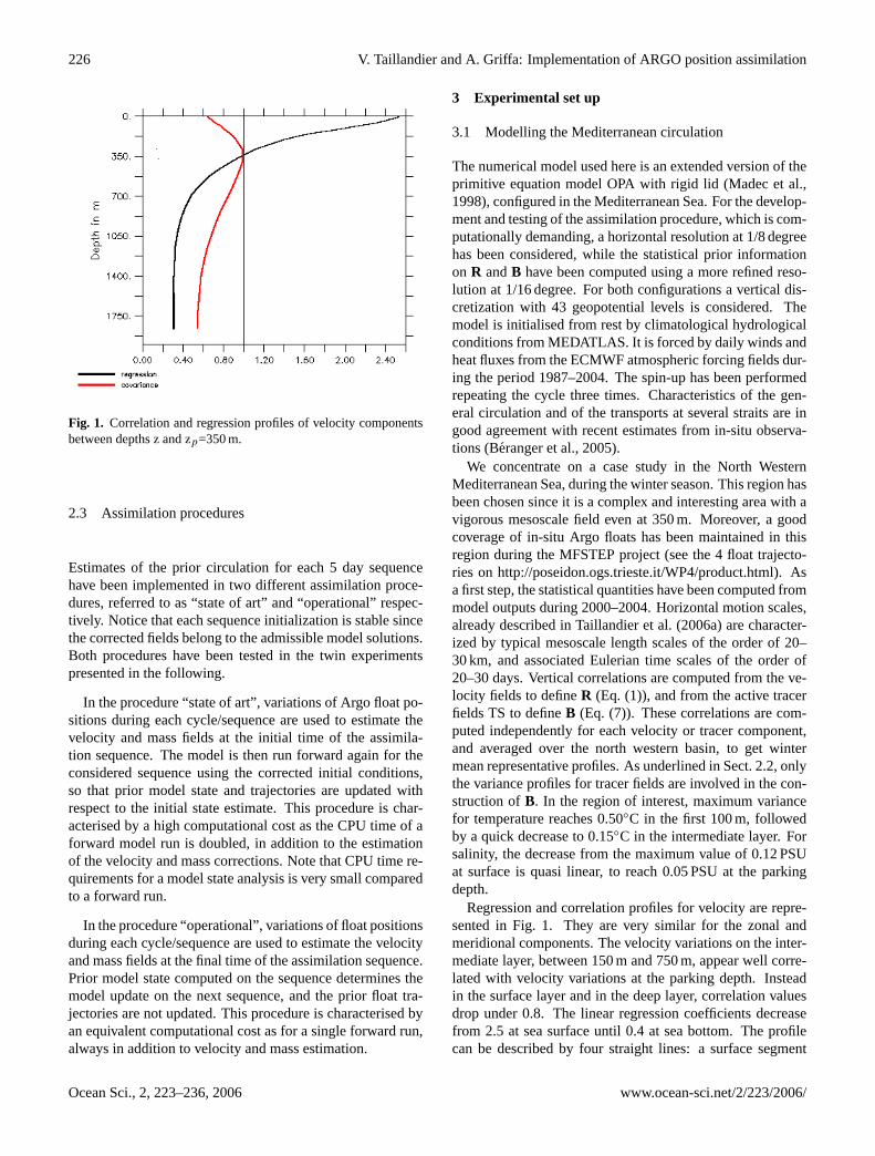
Fig. 6. Profiles of E(z) at the end of the assimilation period for P = 182 (top), 42 (middle), 9 (bottom), for the procedure “state of art” (left)and “operational” (right). Adjustment errors of the vertical mean velocity are indicated in straight lines.

comparing the results in the left and right panels of Fig. 6.As it can be seen, results at the parking depth (discussed inSect. 4.1) appear to hold also for an extended layer between150 m and 500 m. For both procedures, the adjustment errorsincrease at the sea surface and in the deep layer. With lowdata coverage, this growth is limited and the results of the twoprocedures are similar. On the other hand, when the coverageis high (P equal to 182, 42), the growth of E(z) at depth is lim-ited (∼20%) with the “state of art” procedure while is higherin the “operational” procedure (∼35%). Notice that adjust-ments of vertical mean currents are of same order for bothprocedures. In order to better visualize the TS correction,a hydrologic section is extracted along the NW-SE transectshown in Fig. 5. The background, truth and estimated massfields given at the end of the assimilation period are presentedin Fig. 7 for the case of P equal to 42. Note that estimates ofthe mass field and of the horizontal velocity (Fig. 5) are ob-

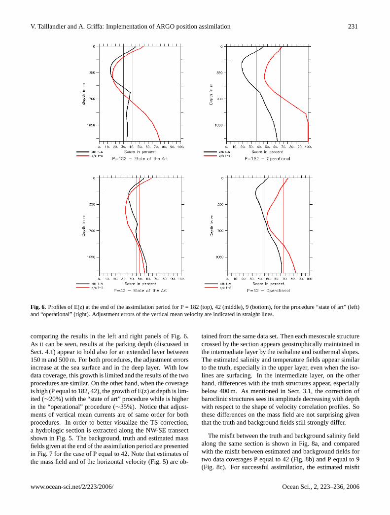
tained from the same data set. Then each mesoscale structurecrossed by the section appears geostrophically maintained inthe intermediate layer by the isohaline and isothermal slopes.The estimated salinity and temperature fields appear similarto the truth, especially in the upper layer, even when the iso-lines are surfacing. In the intermediate layer, on the otherhand, differences with the truth structures appear, especiallybelow 400 m. As mentioned in Sect. 3.1, the correction ofbaroclinic structures sees its amplitude decreasing with depthwith respect to the shape of velocity correlation profiles. Sothese differences on the mass field are not surprising giventhat the truth and background fields still strongly differ.

The misfit between the truth and background salinity fieldalong the same section is shown in Fig. 8a, and comparedwith the misfit between estimated and background fields fortwo data coverages P equal to 42 (Fig. 8b) and P equal to 9(Fig. 8c). For successful assimilation, the estimated misfit

www.ocean-sci.net/2/223/2006/ Ocean Sci., 2, 223–236, 2006

232 V. Taillandier and A. Griffa: Implementation of ARGO position assimilation

Fig. 7. Temperature in◦C (left) and salinity in PSU (right) along the hydrologicSect. (see Fig. 5) at the end of the assimilation period for thebackground (top), truth (middle) and estimate with P=42 (bottom).

is expected to converge toward the truth misfit. In the upperlayer the structures appear well reproduced for both cover-ages, even though for P equal to 9 the intensity is underes-timated. Moreover, each surface misfit appears balanced inthe subsurface, which contributes to the differences obtainedin the intermediate layer, Fig. 7. Such mechanism is accen-tuated at low data coverage, and it can be related to the weakadjustment of baroclinic structures obtained with P equal to 9(as shown Fig. 6, lower panels). In Fig. 8c, the hydrologicalpatterns appear only estimated locally. At each of these loca-tions, the water column sees its stratification translated verti-cally to generate isopycnal slopes in geostrophic equilibriumwith the velocity correction. In consequence, the resultingdensity anomaly at the surface layer is balanced at depth.

In summary, the results show that the assimilation is effec-tive. Velocity estimates at the parking depth converge towardthe truth at increasing coverage. At depth the adjustment iseffective in a large intermediate layer (from 100 m to 700 m)for high coverage, while it is weaker and more homogeneousfor lower coverage. The TS correction is in good agreement

with the truth mass field, especially in the surface and inter-mediate layers, even for low coverage. Notice that improvedadjustments in the surface layer would also be consecutiveto the positive effect of unperturbed forcing fields (heat andmomentum fluxes). The “operational” procedure, with a re-duced CPU cost, appears to perform satisfactorily, providedthat the active TS correction (Sect. 2.2) is performed.

5 Assimilation skills with realistic Argo type data

In this set of simulations, data with realistic characteristicswith respect to Argo floats are considered. On the basis ofprevious results in Sect. 4, only the operational procedure isconsidered.

Results presented in the previous Sect. 4 were obtainedusing perfect positions, extracted at the parking depth. Here,instead, realistic surface data positions are considered, ac-counting for the “observational error” induced by shear drift.The methodology used for assimilation is the same as for per-fect data, except that now the background trajectories used to

Ocean Sci., 2, 223–236, 2006 www.ocean-sci.net/2/223/2006/

V. Taillandier and A. Griffa: Implementation of ARGO position assimilation 233

Fig. 8. Salinity misfits (in PSU) along the hydrologic section(seeFig. 5) at the end of the assimilation period: truth minus background(a); estimate minus background with P=42(b) and with P=9(c).

estimate the velocity at the parking depth (Sect. 2.1) containascent and descent motions at each sequence. Accounting forvertical motions is expected to provide prior information onthe shear error, in the sense that the effects of shear are effec-tively inserted in the cost function (defined in Taillandier etal., 2006a) similarly to the classical specification of observa-tion error covariances (Talagrand, 1999).

Adjustment errors E(t) computed at the parking depth inpresence of this observational error are presented in Fig. 9afor P equal to 182, 42, 9. They can be compared with the

Fig. 9. Evolution of the adjustment error E(t) at the parkingdepth computed from realistic surface data with different coverage:P=182, 42, 9(a), and P=3, 4(b).

results in Fig. 4 obtained with perfect datasets. With lowdata coverage (P equal to 9 and 42), the evolution of E(t) isvery close to that obtained with perfect datasets, with min-imum values of 70% and 40% respectively obtained at theend of the assimilation period. In case of high data coverage(P equal to 182), on the other hand, the E decrease is quicklyreduced after the third sequence. Its minimum is approxi-mately 40%, while in the case of perfect data E(t) reached20%. This different behaviour can be explained consideringthat datasets of low coverage provide information of coarseresolution on the truth circulation, while shear errors haverelatively small amplitudes (about 19% of the drift at parkingdepth) and would affect only fine scale information. In con-sequence, the obtained velocity estimates for low coverage

www.ocean-sci.net/2/223/2006/ Ocean Sci., 2, 223–236, 2006

234 V. Taillandier and A. Griffa: Implementation of ARGO position assimilation

Fig. 10. Velocity misfits (in m/s) at the parking depth at the end ofthe assimilation period: truth minus background(a); estimate withP=3 minus background(b).

are likely to be less sensitive to the introduction of shear er-rors which only affect high resolution datasets.

A second characteristic of Argo floats concerns their typ-ical spatial coverage. For example, there are typically threeto six active floats in the North Western Mediterranean Seain the framework of the MFSTEP project. So the simulateddata sets have to be reduced to few trajectories. Correspond-ing adjustment errors E(t) are represented in Fig. 9b for Pequal to 3 and 4. E(t) decreases in average indicating thatthe assimilation is effective, but the evolution appears nonmonotonous, especially for P equal to 3, with variations be-tween sequences of the order of 5%. Minimum E valuesreached during the one month assimilation are between 85%and 95%.

Such a global assessment needs to be refined in order tounderstand what could be expected in the assimilation of realArgo data positions. In order to have a more detailed, eventhough qualitative assessment, we consider a horizontal map

at the parking depth of the truth minus background misfit(utru – ubck) at the end of the integration and we compare itwith the estimate minus background misfit (uest – ubck) ob-tained with P equal to 3. The corresponding fields and floatstrajectories are shown in Fig. 10. A visual comparison showsthat the assimilation tends to reproduce correctly the mainstructures, at least in the areas where data are available. Thethree floats sample different regions and have different im-pacts on the assimilation process. The most western float islocated in a very energetic area. It is therefore characterizedby important displacements. The other two floats are locatedin a more quiescent region, with meandering motion and re-duced displacements. For the energetic float, the structuresof velocity corrections obtained at each sequence appear topropagate quickly south-westward, as indicated by the struc-ture situated north of the Balearic Islands. The propagation islikely to be due to a combination of advection processes andpropagation of Rossby modes that are prominent in this area(Pinardi and Navarra, 1993). As a consequence, the velocitycorrections which persist in the map (Fig. 10b) are mostlyperformed at the final sequences. Thus the global adjustmenterror E(t) quickly reaches its threshold value. For the lessenergetic floats in the central basin, on the other hand, thelocal velocity correction appears less influenced by propa-gation. As the floats stay longer in the same zone, velocityestimates obtained at the end of the assimilation period resultfrom the whole sequences of analysis. Particularly, the east-ern trajectory infers a major correction on the backgroundcirculation to relocate northward the flow path. The trajec-tory located at the centre, which starts with slow displace-ments to finish with larger ones, leads to velocity correctionspartially propagating westward where they contribute to thecorrection inferred by the previous float. Another part of thecorrection does not appear to move, and it leads to a localcorrection which is not in complete agreement with the truthminus background misfit at the end of the assimilation pe-riod.

6 Summary and concluding remarks

An assimilation method for Argo float positions has beendeveloped and implemented. Investigations have been per-formed in a realistic model configuration of the Mediter-ranean Sea focusing on the North Western area. A first set ofexperiments have been performed to test the method in idealconditions. Perfect data with no shear error are considered,corresponding to the initial and final positions of each cycledrift at the parking depth zp. Relatively high coverages areconsidered, with a number of floats P ranging between 182and 9. Two different procedures are tested: a “state of art”one, where for each sequence the analysis is performed atinitial time and the model is re-run forward starting from thecorrected initial conditions; and an “operational” one where

Ocean Sci., 2, 223–236, 2006 www.ocean-sci.net/2/223/2006/

V. Taillandier and A. Griffa: Implementation of ARGO position assimilation 235

the analysis is performed at final time and the model is notre-run forward on the sequence.

The results show that the assimilation is effective for bothprocedures. The velocity field estimated at zp converges to-ward the truth at increasing coverage. The global adjustmenterror E, computed over the region of interest, ranges between20% for P equal to 182 and 70% for P equal to 9 after onemonth of assimilation. The correction projected in the watercolumn is effective in a thick intermediate layer around zp.For deeper layers or lower coverage (P equal to 9) the correc-tion is lower but still significant, with values around E=70%.Also the correction of the mass field TS appears significantand consistent, even for low coverage. The performance ofthe two procedures is similar, provided that the mass field isestimated as discussed in Sect. 2.2. Only when TS are notactively corrected (and let free to evolve and passively cor-rect themselves), the “operational” procedure appears signif-icantly less effective. Given that the “operational” procedurehas a lower CPU cost and it is more compatible with stan-dard procedures for the assimilation of other data sets, weconsider it more convenient and we recommend it for futureapplications.

A second set of tests have been performed (with the “oper-ational” procedure only) using data with realistic character-istics, with the goal of investigating the potential impact ofArgo floats in observing systems. Realistic position data areconsidered, i.e. taken at the surface and therefore contami-nated by shear errors. The results are compared with thosefor perfect data with P equal to 182, 42, 9. Accounting forshear errors shows a significant impact for high coverage,P equal to 182, increasing the final adjustment E from 20%to 40%. For lower coverage, the impact appears negligible,possibly because its fine scale effect is masked by the coarseresolution of the datasets used to describe the truth circu-lation. We have then considered the impact of realisticallylow coverage, considering P equal to 4, 3. The assimilationappears effective in the sense that the global adjustment er-ror E(t) tends to decrease in average, even though its finalvalue is high, of the order of 85–95%. Locally, the assimila-tion effectively corrects the mesoscale structures sampled bythe data. Even when the correction propagates dynamically(through advection and wave propagation) in regions with nodata, it correctly modifies the model circulation with respectto the truth. Of course, as for any sparse dataset, the possi-bility of having spurious corrections in regions of data voidspersists and it would be reinforced with longer experimentaldurations. Still after one month, this phenomenon appearsvery limited at least in the performed experiments, possiblybecause of the dynamically balanced nature of the correction.

In summary, the present results indicate that the assimila-tion of realistic Argo floats, despite shear error and sparse-ness, can provide significant corrections to model solutionsand help converging toward the truth. These results are con-firmed by a recent work by Taillandier et al. (2006b), wherein-situ Argo data from the MFSTEP project in the Mediter-

ranean Sea have been assimilated in the OPA model in thesame region considered here. In the case of in-situ data, re-sults cannot be tested against the truth which is obviously un-known. Nevertheless, the corrections appear significant andconsistent with Argo float measurements and, at least quali-tatively, also with independent current-meter measurements.

We notice that an intrinsic limit to the use of Argo datapositions is the fact that the time interval1t between succes-sive observations is of the order of the typical Lagrangiantime scale TL. This implies that the details on the struc-ture curvature are not contained in the data. In the presentruns, we have not encountered any major problem relatedto this, differently from the previous work by Taillandier etal. (2006a) where floats in a strong vortex appeared to leadto spurious velocity corrections. This is probably due tothe fact that in Taillandier et al. (2006a) the velocity fieldwas reconstructed from float data alone, without assimilatingthem in a model, while here accounting for model dynam-ics helps providing additional information on the structures.On the other hand, even though no catastrophic event occursin the present experiments, the float correction is in generalless significant for structures of high curvature, such as smalland intense vortices, with respect to circulation features withbroader scales, such as major currents or meanders. This canbe seen also in the assimilation of in-situ data (Taillandieret al., 2006b). When the floats enter strong currents andjets with long time and space correlations, the velocity cor-rection is strong and consistent, while when floats loop insmall structures such as submesoscale vortices (Testor andGascard, 2003; Testor et al., 2005), the correction is weaker.

As a final remark we notice that, even though the presentresults are very positive, some aspects persist that can befurther investigated and improved in future works. First ofall, we notice that the results strongly depend on the statisti-cal correlations used for projection of the velocity correctionin the water column. While in the North Western Mediter-ranean Sea considered here the velocity correlation profilesappear well represented, it can be expected that in regionswith higher variability and baroclinicity the approach mightbe less successful. Also, the use of the geostrophic balancein the mass correction limits the validity of the method tomesoscale open ocean or shelf flows. In principle, a pow-erful alternative to the statistical projection and simplifieddynamics used here is a constraint based on the full modeldynamics (e.g., Nodet, 2006). The counterpart is that thenumber of variables and parameters to be fitted to the data ismuch higher. So, for a reduced data set as for Argo floats,the choice of the most effective method is expected to be acompromise between the complexity of the considered dy-namics and the type of available information. Finally, Argofloats measure also vertical profiles of temperature and salin-ity and the simultaneous assimilation of such TS profiles andpositions would be a promising avenue for future works.

www.ocean-sci.net/2/223/2006/ Ocean Sci., 2, 223–236, 2006

236 V. Taillandier and A. Griffa: Implementation of ARGO position assimilation

Acknowledgements.This work was supported by the EuropeanCommission (V Framework Program – Energy, Environmentand Sustainable Development) as part of the MFSTEP project(contract number EVK3-CT-2002-00075) and by the Office ofNaval Research grant N00014-05-1-0094. We wish to gratefullythank A. Bozec, K. Beranger, L. Mortier for their assistance, P. DeMey, A. Molcard, T.Ozgokmen for useful discussions. Thanks tothe MERCATOR project which provided the numerical model andthe forcing from ECMWF.

Edited by: D. Webb

References

Beranger, K., Mortier, L., and Crepon, M.: Seasonal variability oftransports through the Gibraltar, Sicily and Corsica straits from ahigh resolution Mediterranean model, Prog. Oceanogr., 66, 341–364, 2005.

Gilbert, J.-C. and Lemarechal, C.: Some numerical experimentswith variable-storage quasi-Newton algorithms, Math. Program.,45, 407–435, 1989.

Ide, K., Kuznetsov, L., and Jones, C. K. R. T.: Lagrangian dataassimilation for point vortex systems, J. Turbul., 3, 53–59, 2002.

Ishikawa, Y. I., Awaji, T., and Akimoto, K.: Successive correctionof the mean sea surface height by the simultaneous assimila-tion of drifting buoys and altimetric data, J. Phys. Oceanogr., 26,2381–2397, 1996.

Jackett, D. R. and McDougall, T. J.: Minimal adjustment of hy-drographic profiles to achieve static stability, J. Atmos. Ocean.Tech., 12, 381–389, 1995.

Kamachi, M. and J. O’Brien: Continuous assimilation of driftingbuoy trajectory into an equatorial Pacific Ocean model, J. Mar.Syst., 6, 159–178, 1995.

Kutsnetsov, L., Ide, K. and Jones, C. K. R. T.: A method for assim-ilation of Lagrangian data, Mon. Weather Rev., 131, 2247–2260,2003.

Madec, G., Deleucluse, P., Imbard, M., and Levy, C.: OPA8.1 oceangeneral circulation model reference manual, Technical ReportLODYC/IPSL [http://www.lodyc.jussieu.fr/opa], 1998.

Molcard, A., Griffa, A., andOzgokmen, T.: Lagrangian data assim-ilation in multilayer primitive equation models, J. Atmos. Ocean.Tech., 22, 70–83, 2005.

Molcard, A., Piterbarg, L. I., Griffa, A.,Ozgokmen, T. M., andMariano A. J.: Assimilation of drifter positions for the recon-struction of the eulerian circulation field, J. Geophys. Res., 108,3056, 2003.

Molcard, A., Poje, A. J., andOzgokmen, T. M.: Directed drifterlaunch strategies for Lagrangian data assimilation using hyper-bolic trajectories, Ocean Model, 12 (3–4), 268–289, 2006.

Nodet, M.: Variational assimilation of Lagrangian data in oceanog-raphy, Inverse Probl., 22, 245–263, 2006.

Oschlies, A. and Willebrand, J.: Assimilation of Geosat altime-ter data into an eddy-resolving primitive equation model of theNorth Atlantic Ocean, J. Geophys. Res., 101, 14 175–14 190,1996.

Ozgokmen, T. M., Molcard, A., Chin, T. M., Piterbarg, L. I., andGriffa, A.: Assimilation of drifter positions in primitive equationmodels of midlatitude ocean circulation, J. Geophys. Res., 108,3238, 2003.

Park, J. J., Kim, K., King, B. A., and Riser, S. C.: An advancedmethod to estimate deep currents from profiling floats, J. Atmos.Ocean. Tech., 22, 1294–1304, 2005.

Pinardi, N. and Navarra, A. : Baroclinic wind adjustment processesin the Mediterranean Sea, Deep Sea Research II, 40, 1299–1326,1993.

Pinardi, N., Allen, I., Demirov, E., De Mey, P., Korres, G., Las-caratos, A., Le Traon, P.-Y., Maillard, C., Manzella, G., andTziavos, C.: The Mediterranean ocean forecasting system: firstphase of implementation (1998–2001), Ann. Geophys.,21, 3–20,2003.

Poulain, P. M.: MEDARGO: A profiling float program in theMediterranean, Argonautics, 6, 2, 2005.

Raicich, F. and Rampazzo, A.: Observing system simulation exper-iments for the assessment of temperature sampling strategies inthe Mediterranean Sea, Ann. Geophys., 21, 151–165, 2003.

Taillandier, V., Griffa, A., and Molcard, A.: A variational approachfor the reconstruction of regional scale Eulerian velocity fieldsfrom Lagrangian data, Ocean Model., 13, 1, 1–24, 2006a.

Taillandier, V., Griffa, A., Poulain, P.-M., and Beranger, K.: Assimi-lation of Argo float positions in the North Western MediterraneanSea and impact on ocean circulation simulations, Geophys. Res.Lett., in press, 2006b.

Talagrand, O.: A posteriori evaluation and verification of analysisand assimilation algorithms, Proceedings of workshop on “Diag-nostic of data assimilation systems” ECMWF, 1999.

Talagrand, O. and Courtier, P.: Variational assimilation of meteo-rological observations with the adjoint vorticity equation, Q. J.Roy. Meteor. Soc., 113, 1311–1328, 1987.

Testor, P. and Gascard, J.-C.: Large-scale spreading of deep wa-ters in the Western Mediterranean Sea by submesoscale coherenteddies, J. Phys. Oceanogr., 33, 75–87, 2003.

Testor, P., Beranger, K., and Mortier, L.: Modelling the eddy fieldin the South Western Mediterranean: the life cycle of Sardinianeddies, Geophys. Res. Lett., 32, L13602, 2005.

Toner, M., Poje, A. J., Kirwan, A. D., Jones, C. K. R. T., Lipphardt,B. L., and Grosch, C. E.: Reconstructing basin-scale Eulerianvelocity fields from simulated drifter data, J. Phys. Oceanogr.,31, 1361–1376, 2001.

Ocean Sci., 2, 223–236, 2006 www.ocean-sci.net/2/223/2006/