Imperfect competition, demand uncertainty

and capacity adjustment

Werner Smolny, University of Ulm and ZEW Mannheim

March 26, 2004

Abstract:

In this paper a theoretical model of the price versus quantity adjustment of the

firm is developed. The model is characterized by short-run capacity constraints,

uncertainty about demand and imperfect competition on the product market. The

microeconomic model is complemented by aggregation. The aggregate model exem-

plifies the prominent role of capacity utilization as a business cycle indicator and

yields a variant of an accelerator model for the capacity adjustment. The demand

and cost multipliers depend on the share of capacity constrained firms, and the price

adjustment is determined by unit labour costs, capacity utilization and competition.

Keywords: Imperfect competition, demand uncertainty, capacity adjustment

JEL No.: D21, D40, E22, E32

Address: Prof. Dr. Werner Smolny

Ludwig Erhard Chair

Faculty of Mathematics and Economics

Department of Economics

University of Ulm

89069 Ulm, GERMANY

Tel.: (49) 731 50 24260, Fax: (49) 731 50 24262

e-mail: Werner.Smolny@mathematik.uni-ulm.de

1 Introduction

The analyses of market structure and macroeconomic fluctuations are related through

the price-setting behaviour of firms. On the one hand, macroeconomic evidence on

cyclical fluctuations and the analysis of price versus quantity adjustments of firms

can reveal insights into the competitive situation on the markets.1 On the other

hand, the analysis of market structure and price adjustment can help to a better

understanding of the propagation of macroeconomic shocks.2 Classical and Key-

nesian models differ with respect to the underlying model of the price adjustment.

In classical models, an immediate or very fast adjustment of prices and permanent

market clearing is assumed. Keynesian models, in contrast, emphasize the relevance

of price rigidities, market disequilibria and quantity reactions. Both models yield

opposite policy implications. Therefore the analysis of price adjustment is important

for macroeconomic analysis.

A convenient framework to analyse price vs. quantity adjustments is monopolistic

competition. Imperfect competition provides a prerequisite for a general theory

of price adjustment.3 The theory of price adjustment is dominated by the idea

that prices adjust in the presence of excess demand or supply on the market. This

mechanism is essentially ad hoc and does not reflect optimizing behaviour. In ad-

dition, it requires a disequilibrium interpretation of the adjustment which is not

compatible with perfect competition. Monopolistic competition, by itself, cannot

explain why aggregate demand movements affect output,4 but monopolistic compe-

tition combined with some other imperfection can explain the interrelation of real

and nominal variables. The main imperfection which is analysed here is a dynamic

adjustment of capacities and technology. It is assumed that capacities adjust only

1See Hall (1986) and Carlton (1989).2See Mankiw (1985), Hall (1986), Blanchard and Kiyotaki (1987), Solow (1998) and Ellison and

Scott (2000).3See Barro (1972).4See Blanchard and Kiyotaki (1987).

2

with a delay with respect to cost and demand changes, thus under uncertainty about

demand.5 The analysis of a dynamic adjustment permits the consistent introduction

of capacity constraints and uncertainty into the model.

The short-run price and quantity adjustment is analysed within a model of monop-

olistic competition on the product market and short-run capacity constraints. An

extended model introduces a delayed adjustment of prices and employment with

uncertainty about demand. This medium-run model provides a framework to anal-

yse short-run price rigidities combined with constraints on the adjustment of em-

ployment. The model can account for delivery lags and labour hoarding during

recessions, i.e. it is consistent with a procyclically varying productivity of labour.

The capacity adjustment is analysed within the long-run model. For the capacity

decision, the optimal response of prices, output and employment with respect to

demand shocks is taken into account. The model yields an accelerator mechanism

for the capacity adjustment. It is shown that the inefficiency associated with a de-

layed adjustment of capacities and demand uncertainty exhibits the same effects on

optimal capacities, capital-labour substitution and average prices as higher capital

costs.

The model of the firm is complemented by aggregation. The microeconomic relations

at the firm level are explicitely translated into macroeconomic relations between the

aggregates. In addition, the equilibrium shares of firms with supply and demand

constraints are determined. The aggregate model exemplifies the role of capacity

utilization as business cycle indicator; capacity utilization determines both the ad-

justment of prices and employment in the medium run and capital investment in the

long run. The price adjustment depends on supply and demand shocks according to

a short-run Phillips curve mechanism. The extend of price vs. quantity adjustments

is determined by capacity utilization. This implies an asymmetric price and quantity

5For the analysis of adjustment delays see Kydland and Prescott (1982) and Pacheco-de-Almeida

and Zemsky (2003). The model here is basically an extended variant of the model of Hall (1986).

3

adjustment with respect to demand and cost shocks during the business cycle.

2 Assumptions

In the theoretical model a strong separability of the dynamic structure of the firm’s

decisions is assumed. In the short run, output, employment and prices are endoge-

nous. In the long run, the firm decides on investment and the production technology,

i.e. capacities and the production technology adjust only with a delay with respect to

demand and cost changes, thus under uncertainty about demand.6 As an extention,

a delayed adjustment of prices and employment is discussed. In most adjustment

models dynamics are analysed under the assumption of non-linear adjustment costs.

However, it is difficult to find examples for adjustment costs which can account

for the observed slow adjustment of many economic variables. On the other hand,

changing decision variables necessarily takes time, and even a short delay between

the decision to change capacities or the price and the realization of a demand shock

can introduce considerable uncertainty. In addition, the analysis of the dynamic

adjustment in terms of adjustment delays and uncertainty reduces the dynamic de-

cision problem of the firm to sequential static decision models which can be solved

stepwise.

The theoretical analysis is carried out within a framework of monopolistic compe-

tition on the product market.7 Imperfect competition is firstly a prerequisite for

the analysis of price change. Price adjustment with respect to excess demand and

supply requires a disequilibrium interpretation which is not compatible with perfect

competition. In addition, the introduction of capacity constraints and demand un-

certainty implies a monopolistic adjustment of the firms operating on the market at

least in the short run. Finally, fixed costs of production and increasing returns to

6For a discussion of adjustment delays, see Kydland and Prescott (1982) and Pacheco-de-Almeida

and Zemsky (2003).7See e.g. Barro (1972) and Dixit and Stiglitz (1977).

4

scale associated with for instance innovations or advertising provide further argu-

ments for a monopolistic market structure.8 Within the microeconomic analysis, a

market is defined by the supply of a single firm and the demand for the firm’s prod-

uct. In the sequel an aggregation procedure is discussed to derive implications for

macroeconomic relations. In order to distinguish demand shifts, the price elasticity

of demand and demand uncertainty, a log-linear demand curve is assumed,9

lnYD = η · ln p + ln Z + ε, η < −1,E(ε) = 0,Var(ε) = σ2ε . (1)

The time and firm indices are omitted to simplify notation. Demand YD is de-

termined by the price p, exogenous demand shifts Z and a demand shock ε. The

demand shift Z stands for aggregate demand and the market share of the firm which

is determined by, for instance, the prices of other firms, consumer preferences and

the quality of the firm’s product. In the basic model, it is assumed that the re-

alized value of the demand shock ε is known at the time of the output, price and

employment decision, but is not known at the time of the investment decision. In

the extended version, there is uncertainty about ε at the time of the price and

employment decision. In addition, ε exhibits positive autocorrelation. Supply YS

is determined by a short-run limitational production function with capital K and

labour L as inputs,

YS = min(YC, YL) = min(πk · K,πl · L), πl = πl(k, θ), πk = πk(k, θ). (2)

YC are capacities, YL is the employment constraint and πl, πk are the productivities

of labour and capital. It is assumed that the capital stock as well as the factor pro-

ductivities are predetermined in the short run; they are determined by the long-run

investment decision. Adjustment delays for the capital stock arise from planning,

decision, delivery and installation lags for investment, the assumption of short-run

8See for instance Kamien, Schwarz (1975), Scherer and Ross (1990) and Aghion and Howitt

(1992).9Log-linear demand curves can be derived from CES utility functions (Deaton and Muellbauer,

1980), and log-linear relations permit an easy aggregation over firms (Lewbel, 1992).

5

fixed production coefficients corresponds to a putty-clay technology.10 The factor

productivities are determined by the capital-labour ratio k and production efficiency

θ. The factor prices are assumed to be exogenous at the firm level. These assump-

tions imply constant marginal costs within the capacity limit in the short run.

3 Output, prices and employment

3.1 Imperfect competition and capacity constraints

The short-run model corresponds largely to the standard framework of monopolistic

competion, but is extended with capacity constraints.11 The optimization problem

of the firm is

max→p,Y,L

p · Y − w · L − c · K s.t. Y ≤ {YC, YL, YD}. (3)

Supply and demand are determined according to eqs. (1) and (2). w are wages and

c are the user costs of capital. The capital stock and the factor productivities are

predetermined. The first order condition is

p · (1 + 1/η) · (1 − λYC) · πl − w = 0. (4)

λYC is the shadow price of the capacity constraint; it is zero in case of sufficient

capacities. For the optimal solution, two cases can be distinguished:

1. In case of sufficient capacities λYC = 0, prices, output and employment are

determined as

p(w) =w

πl · (1 + 1/η), (5)

ln Y (w) = η · ln p(w) + ln Z + ε and L(w) = Y (w)/πl. (6)

10The analysis of a dynamic adjustment of capacities has a long tradition in empirical investment

models (see Jorgenson, Stephenson, 1967). The assumption of a putty-clay technology became

common with the work of Bischoff (1971).11The model is basically an extended variant of the model of Hall (1986).

6

Optimal prices are determined by unit labour costs and the price elasticity of de-

mand, output results from introducing this price into the demand function, and

employment is the required labour input. The firm suffers from underutilization of

capacities.

2. In case of capacity shortages λYC 6= 0, output, employment and prices result from

Y = YC, L(YC) = YC/πl, (7)

ln p(YC) = (ln YC − lnZ − ε)/η. (8)

Optimal output is equal to the capacity constraint, employment is again given as

the corresponding labour requirement, and the optimal price results from solving

the demand function for p at YD = YC. Insufficient capacities restrain output and

employment, and the firm increases the price.

There is exactly one value of the demand shock ε = ε which distinguishes these

cases,

ε = ln YC − η · ln p(w) − ln Z. (9)

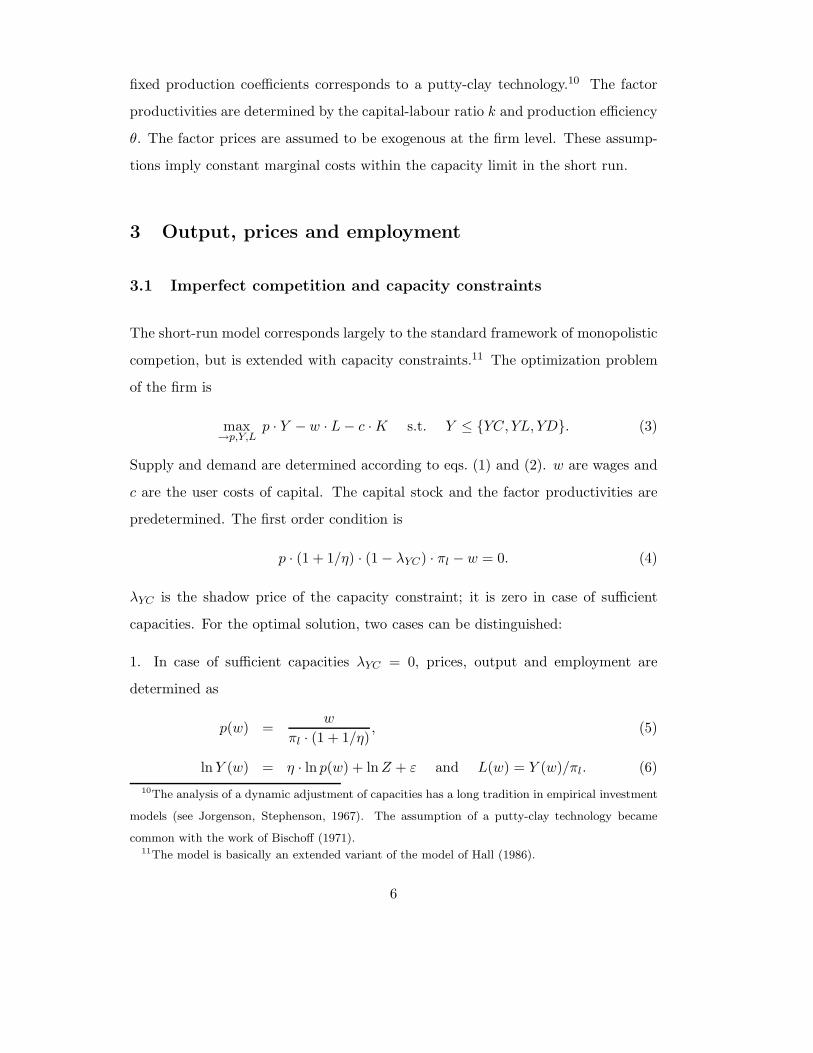
The most important characteristics of the model are the minimum price p(w) and

the capacity limit YC. The supply curve is horizontal within the borders of capacity

and vertical at the capacity limit. Optimal prices are determined either by unit

labour costs and the degree of competition on the market or by the relation of the

levels of demand and capacity. Optimal output and employment are determined

either by unit labour costs and the level of demand or by capacities. Figure 1 gives

a visual impression of the model. For a negative demand shock ε1 < ε, the price is

bounded by unit labour costs and the mark-up. For a positive demand shock ε2 > ε,

insufficient capacities restrain output, and the firm increases the price. ε = ε is the

borderline which distinguishes these cases. Note the implied asymmetry of the price

and quantity adjustment in case of positive and negative demand shocks. A similar

asymmetry results for cost changes.

The microeconomic model of the firm provides a consistent basis for aggregation.

7

Figure 1: Immediate adjustment of output, prices and employment

YC Y

YD(p, ε = ε)

YD(p, ε = ε2)

YD(p, ε = ε1)

p(w)

p ε1 < ε < ε2

If firms differ only with respect to the realization of the demand shocks ε, the

microeconomic minimum condition of supply and demand at the firm level can be

explicitely translated into a macroeconomic relation between the averages and the

variance of demand shocks σ2ε . For instance, if the distribution of ε is approximated

by the Normal, the aggregate relation exhibits the same functional form as the

microeconomic relation, except for a change of the normalizing constant which is

determined by the variance of demand shocks,12

ln E(YD) = E(ln YD) + 0.5 · σ2ε = η · ln p + ln Z + 0.5 · σ2

ε . (10)

E is the expectation operator, n is the number of firms and n · E(YD) is aggregate

demand. If costs, prices and demand shifts differ between firms, the normalizing

constant is determined by the variance of the logarithm of demand at the micro

level.13 In addition, the aggregate counterpart of the microeconomic minimum con-

12See Stoker (1993) for a discussion.13The variance of the logarithm of demand is determined by the variances and correlations of

demand shocks ε, demand shifts Z and prices (costs).

8

dition can accurately be approximated by a CES-type function of aggregate output

n ·E(Y ) in terms of aggegate capacities n ·E(YC) and aggregate demand n ·E(YD),

E(Y )1/ρ ≈ E(YD)1/ρ + E(YC)1/ρ, ρ < 0. (11)

ρ can be interpreted as a mismatch parameter (mismatch between demand and

capacities) with ∂E(Y )/∂ρ < 0 and limρ→0 E(Y ) = min[E(YD),E(YC)]. ρ is com-

pletely determined by the covariance of capacities and demand at the micro level.14

The aggregate multipliers, i.e. the elasticities of aggregate output with respect to

capacities and demand can be calculated from eq. (11) as

∂E(Y )

∂E(YD)·E(YD)

E(Y )≈

{

E(YD)

E(Y )

}1/ρ

≈ prob(YD < YC) (12)

and correspondingly for capacities. These elasticities approximate the shares of

firms with or without capacity constraints. The aggregate model implies that the

demand and cost multipliers depend on the business cycle. In boom situations with

a high capacity utilization and a large share of firms with capacity constraints, prices

adjust with respect to demand with only small output and employment effects and

only small effects from cost changes. In recession periods with a large share of

firms with sufficient capacities, quantities (output and employment) adjust with

respect to demand and cost changes, and prices adjust only with respect to costs.

The microeconomic case dependency of cost and demand effects corresponds to

cyclical demand and cost multipliers at the macro level. For the price adjustment

the aggregate model implies an augmented Phillips curve mechanism: Prices adjust

with respect to unit labour cost (supply shocks) and capacity utilization (demand

shocks). If aggregate demand depends on employment, the model yield the usual

Keynesian multiplier but only within the borders of capacities, i.e. the model exhibits

both classical and Keynesian features.

14ρ is determined by a nearly linear relation in terms of the standard deviation of ln YD − ln YC

within the empirically relevant range.

9

3.2 Uncertainty and the price and employment adjustment

The extended model introduces uncertainty into the price and employment adjust-

ment. It is assumed that prices and employment must be chosen in advance, thus

under uncertainty about demand.15 Adjustment delays for employment can be jus-

tified with legal/contractual periods of notice and search, screening and training

time.16 The assumption that the firm sets price tags also appears plausible,17 and

even a short delay between the decision to change the price and the realization of

demand can introduce considerable uncertainty. In this model, output is determined

in the short run as the minimum of demand and supply,

Y = min(YD, YS). (13)

The medium-run optimization problem is

max→L,p

p · E(Y ) − w · L − c · K (14)

s.t. eqs. (1) and (2) above. Expected output is determined as

E(Y ) = E[min(YD, YS)] =

∫ ε

−∞

YD · fεdε +

∫

∞

εYS · fεdε (15)

fε is the p.d.f. of the demand shock ε. For small values of the demand shock,

output is determined by demand (the first integral); for large values of ε, output is

determined by supply (the second integral); ε is defined as the specific value of the

demand shock ε where demand equals supply,

ε = ln YS − η · ln p − ln Z. (16)

The first order conditions are given by18

η ·

∫ ε

−∞

YD · fεdε + E(Y ) = 0, (17)

p ·

∫

∞

εfεdε · (1 − λYC) · πl − w = 0. (18)

15The medium-run model is discussed in Smolny (1998a,b).16See Hamermesh and Pfann (1996).17See Carlton (1989) and Blinder (1991).18Note that the value of the integrands in eq. (15) at ε = ε are equal.

10

The optimal ε depends only on the price elasticity of demand η and demand uncer-

tainty σε (see appendix A, proposition A.1),

ε = ε(η, σε). (19)

ε and σε also determine the expected utilization of supply Ul := E(Y )/YS and

the optimal probability of demand constraints prob(YD < YS) (see appendix A,

proposition A.2). That means, utilization and the probabilities do not depend on

costs, capacities and expected demand shifts Z. The economic intuition of this

result is that (for given supply and costs) the elasticity of output with respect to the

price is chosen equal to one: With higher prices, demand decreases with elasticity

η; expected output decreases with elasticity η, times the weighted probability that

demand is less than supply. The expected share of output in the demand constrained

case is chosen equal to the inverse of the absolute value of the price elasticity of

demand,19

probw(YD < YS) :=

∫ ε−∞

YD · fεdε∫ ε−∞

YD · fεdε +∫

∞

ε YS · fεdε= −

1

η. (20)

The firm chooses the price to achieve an optimal probability of supply constraints

and an optimal utilization of supply. For optimal prices and employment, two cases

can be distinguished:

1. In case of capacity constraints λYC 6= 0, supply and employment are determined

from capacities and labour productivity,

Y = YL = YC and L(YC) = YC/πl. (21)

The optimal price results from inserting capacities and the optimal ε into eq. (16)

and solving for p,

ln p(YC) =[

ln YC − ln Z − ε(η, σε)]

/η. (22)

19Inserting the definition of expected output, eq. (15), into the first order condition with respect

to prices, eq. (17), yields eq. (20).

11

The price depends on capacities YC, expected demand shifts Z and the optimal ε;

the elasticity of the price with respect to capacities and the demand shift is 1/η; the

price does not depend on costs.

2. In case of sufficient capacities λYC = 0, the optimal price follows directly from the

first order condition with respect to employment, eq. (18). The marginal costs of an

additional unit of employment are equal to the wage rate w. Marginal returns are

determined as the price, multiplied with the productivity of labour and multiplied

with the probability that the additional unit of output can be sold. The mark-up of

prices on unit labour costs is chosen equal to the inverse of the optimal probability

of supply constraints,w

πl · p(w)= prob(YL < YD). (23)

Since the optimal probability of supply constraints is competely determined by de-

mand uncertainty σε and the price elasticity of demand η, the price does not depend

on capacities and expected demand shifts. The firm adjusts quantities with respect

to demand. The optimal price can also be determined from the price elasticity of

demand, unit labour costs and the expected utilization of employment (see appendix

A, proposition A.3),

p(w) =w

Ul · πl · (1 + 1/η). (24)

The inefficiency associated with demand uncertainty and a delayed adjustment ex-

hibits the same effect as higher wage costs. Supply and employment result from

inserting this price and the optimal ε into the definition of ε and solving for supply

YL and employment L,

YL(w) = η · ln p(w) + ln Z + ε(η, σε) and L(w) = YL/πl. (25)

The immediate adjustment (or the absence of uncertainty) is contained as the lim-

iting case σε → 0. Without uncertainty Ul → 1, and the firm can achieve full

utilization of employment. Introducing uncertainty reduces the expected utilization

of employment and exhibits the same effect on prices and employment as higher

12

Figure 2: Optimal employment

Y

YD

w

mcmr

fYD

p(w) · πl · prob(YL < YD)

YL YC2YC1

mr: marginal revenue mc: marginal costs

variable costs. Figure 2 gives a visual impression of the model. fYD is the p.d.f. of

demand. For small values of L and YL, the probability that the marginal unit of

labour will be used is large; the marginal returns of labour exceed marginal costs.

For higher values of YL, the probability that demand exceeds supply decreases, and

the marginal return of labour decreases, a unique optimum is assured. If capacities

restrain supply, the firm increases the price to achieve the optimal probability of

supply constraints and the optimal utilization of supply.

The model extends the standard formulation of monopolistic competition by intro-

ducing uncertainty about demand and medium-run capacity constraints. Ex ante,

the firm sets prices and employment under uncertainty about demand, i.e. the firm

chooses one point in the {p, Y }-diagram (see figure 3). Uncertainty increases the

optimal price and reduces employment through the costs of underutilization of em-

ployment. Relevant for the price setting is the capacity limit YS = YL ≤ YC and the

minimum price p(w). In case of sufficient capacities, there is a clear correspondence

13

Figure 3: Delayed adjustment of prices and employment

YL YC Y

YD(p, ε = ε2)

YD(p, ε = ε1)

wπl·(1+1/η)

p(w)

p

ε1 > ε2

of income distribution shares, the price elasticity of demand and the probability

of demand constraints; in case of capacity constraints, the relation of the demand

shift Z and capacities YC determines the optimal price. Ex post, rationing of de-

mand or underutilization of employment can occur. For a positive demand shock

ε = ε1, the firm cannot satisfy all customers (delivery lags), for a negative demand

shock ε = ε2, underutilization of capacities and labour hoarding occur. Short-run

demand shocks can be identified from the utilization of the production factors. The

short-run demand situation can be identified from the utilization of employment,

the medium-run business-cycle situation can be identified from the utilization of

capacities.

The extention of the model also enhances the macroeconomic interpretation of the

effects of imperfect competition and capacity constraints.20 The assumption of a

delayed adjustment of prices introduces demand uncertainty, price rigidities and

20The aggregate counterparts of the microeconomic relations can again be derived from the ag-

gregation procedure discussed above.

14

prolonged delivery lags in the short run. It also permits a discussion of wage-price

patterns and a staggered price setting for the analysis of the aggregate price adjust-

ment.21 The assumption of a delayed adjustment of employment permits an inter-

pretation of the procyclical development of labour productivity in terms of optimal

labour hoarding during recessions. Finally, the assumption of a slow adjustment of

prices and employment introduces dynamics into the multiplier process.

4 Capacities and capital-labour substitution

In the long run, the firm decides on capacities and the production technology. Since

there is uncertainty about the demand shock ε, the realized future values of output,

prices and employment are not known at the time of the investment decision. How-

ever, the firm knows the decision rule for those variables. They are given by the

solutions of the short- and medium-run optimization problems. The capacity ad-

justment is firstly analyzed within the model of the short-run adjustment of output,

employment and prices. The deviations caused by a delayed adjustment of prices

and employment are discussed afterwards.

4.1 Demand uncertainty and capacity adjustment

The firm maximizes expected profits which depend on expected sales, expected em-

ployment, the wage rate and capital costs. The production function is characterized

by constant returns to scale. The decision variables are the capital stock K and the

capital-labour ratio k. The optimization problem is

max→K,k

∫ ε

−∞

(

p(w) −w

πl

)

· Y (w) · fεdε +

∫

∞

ε

(

p(YC) −w

πl

)

· YC · fεdε − c · K. (26)

Output, prices and employment are determined from eqs. (5)-(8). Output is deter-

mined by demand in case of sufficient capacities or by capacities in case of sufficient

21See e.g. Blanchard (1987).

15

demand. Sales result from introducing the corresponding prices, and employment

is given by the labour requirement. ε and fε refer to uncertainty about demand at

the time of the investment decision. The first order condition with respect to the

capital stock K is22

∫

∞

ε[p(YC) · (1 + 1/η) − w/πl] · πk · fεdε − c = 0. (27)

Marginal costs are given by the user costs of capital c. Marginal returns to capital

are achieved only, if capacities become the binding constraint for output, i.e. if

ε > ε. They are given by the price, minus the price reduction of a marginal increase

in output, minus wage costs in the capacity constrained case. A unique optimum

exists, p(YC) is decreasing in YC and K.23 The following properties can be derived.

The optimal value of ε depends only on the price elasticity of demand, the variance

of demand shocks and relative factor costs (see appendix B, proposition B.1),

ε = ε

(

η, σε,c

πk

πl

w

)

. (28)

ε and σε, in turn, determine both the probability of demand constraints prob(YD

< YC) and the expected utilization of capacities Uc := E(Y )/YC (see appendix

B, proposition B.2). Higher relative capital costs increase optimal utilization and

reduce the probability of demand constraints; with high fixed costs, the firm chooses

a higher probability of capacity constraints. More competition, i.e. a higher absolute

value of the price elasticity of demand |η| also increases optimal utilization and

reduces the probability of demand constraints. Both, higher relative capital costs

and more competition increase the ratio between marginal costs and marginal returns

of capital. More uncertainty reduces optimal utilization, because it becomes more

difficult to achieve a higher utilization, and the probability of demand constraints

increases.24 Both, expected capacity utilization and the probabilities of capacity

constraints do not depend on expected demand shifts Z and the level of factor

22The value of both integrands in eq. (26) at ε = ε is equal.23The integrand is equal to 0 at the lower border of the integral.24σε affects the relation between average p(YC) and p(w).

16

costs. The choice of capacities can be understood as the optimal choice of capacity

utilization.

Expected prices E(p) are determined as mark-up over labour and capital costs (see

appendix B, proposition B.3), the average price depends also on the expected uti-

lization of capacities (see appendix B, proposition B.4),

E(p · Y )

E(Y )=

(

w

πl+

c

Uc · πk

)

/(1 + 1/η). (29)

More uncertainty reduces the expected utilization of capacities; a lower utilization

of capacities, in turn, exhibits the same effect on average prices as higher capital

costs c. Finally, optimal capacities are determined as25

ln YC = η · ln p(w) + ln Z + ε. (30)

Optimal capacities depend on expected demand shifts Z, demand shifts increase all

quantities proportionally and do not affect prices or relative quantities. This implies

an accelerator mechanism for the capacity adjustment. Higher relative capital costs

reduce capacities through the optimal value of ε. A proportional increase in c and

w leaves ε, the probabilities and capacity utilization unchanged, but increases the

price proportionally. Capacities decrease with elasticity |η|, the model exhibits linear

homogeneity both in prices and quantities. Less competition reduces capacities

through higher prices and through a lower optimal utilization, and more uncertainty

reduces optimal capacities through a lower utilization. Demand uncertainty exhibits

the same effect on capacities and average prices as higher capital costs. The model

without uncertainty is contained for σε → 0 and Uc → 1. Without uncertainty the

price is set as a mark-up over total costs, and the mark-up is determined by the price

elasticity of demand; optimal capacities and employment are given by the equality

of demand YD, capacities YC and the corresponding employment constraint YL.

The second component of the investment decision is the choice of the optimal capital-

labour ratio k. The capital-labour ratio, in turn, determines the productivities of

25Eq. (30) results from inserting eq. (28) into eq. (9) and solving for YC.

17

labour and capital πl, πk. The optimal capital-labour ratio can be derived from

differentiating eq. (26) with respect to k. The calculations are tedious but not

difficult, and the result is intuitive: The optimal relation between the elasticities

of the factor productivities of labour and capital with respect to the capital-labour

ratio is chosen equal to the ratio of the corrected factor shares,26

−

∂πk

∂k · kπk

∂πl

∂k · kπl

=w · Uc

c

πk

πl. (31)

Again, the inefficiency caused by uncertainty and a delayed adjustment exhibits

the same effects as higher capital costs and favours substitution of labour against

capital; the model without uncertainty is contained for σε → 0 and Uc → 1.

The assumption of a delayed adjustment of capacities and capital-labour substi-

tution extends the deterministic model by introducing uncertainty and permits to

analyse the resulting inefficiencies. Ex ante, the firm chooses capacities and the

factor productivities under uncertainty about demand. With uncertainty, optimal

capacities and expected output are lower due to the costs of stochastic underutiliza-

tion of capacities. Uncertainty also increases average prices and reduces the optimal

capital-labour ratio through the effect on utilization. The optimal probabilities of

capacity constraints, the optimal utilization of capacities and the optimal capital-

labour ratio do not depend on the level of costs and the level of demand. They are

determined by relative costs, demand uncertainty and the price elasticity of demand.

The model exhibits linear homogeneity both in prices and in quantities. Ex post,

capacity and demand constraints on the goods market are possible. The demand

multiplier depends on the share of firms with capacity constraints.

26In case of a Cobb-Douglas production function, this relation is equal to the relative output elas-

ticities of the factors, see appendix C. The appendix also contains the results for a CES production

function

18

4.2 A three-step decision structure

The capacity adjustment can also be analysed in combination with uncertainty about

demand for the price and employment adjustment. Let us assume uncertainty about

the demand expectations at the time of the price and employment decision, i.e.

uncertainty about the expected demand shift Z,

ln Z = ln Z + z, E(z) = 0,Var(z) = σ2z . (32)

z measures the difference of demand expectations at the time of the investment

decision and the time of the price and employment decision. Prices and employment

then depend on the realized value of z. In particular, employment and prices are

determined either from eqs. (21) and (22) in the capacity constrained case or from

eqs. (24) and (25) in the unconstrained case. There is exactly one value z = z which

distinguishes these cases,

z = ln YC − ln Z − ε − η · ln p(w). (33)

Expected employment is determined as

E(L) =

∫ z

−∞

L(w) · fzdz +

∫

∞

zL(YC) · fzdz (34)

fz is the p.d.f. of z. Expected output can be determined from expected employment

and the expected utilization of employment, E(Y ) = Ul · πl · E(L). Expected sales

result as E(p ·Y ) = Ul ·πl ·E(p ·L). Note that the expected utilization of employment

is completely determined by the price elasticity of demand η and demand uncertainty

at the time of the price and employment decision σε, i.e. it is not stochastic and

does not depend on the capacity decision.27 The long-run optimization problem can

be written as28

max→K

∫ z

−∞

[(p(w) · πl · Ul − w] · L(w) · fzdz

27Note that ε and the probabilities on the product market are also determined by η and σε, i.e.

they are also not stochastic and do not depend on the capacity decision.28See eq. (26) for comparison.

19

+

∫

∞

z[p(YC) · πl · Ul − w] · L(YC) · fzdz − c · K. (35)

This formulation of the optimization problem shows that the solution of the model

can be performed correspondingly to the basic model of section 4.1. The first order

condition with respect to the capital stock is given by29

∫

∞

z[p(YC) · (1 + 1/η) · Ul − w/πl] · πk · fzdz − c = 0. (36)

Note that capacities affect output, prices and employment only if capacities are the

binding constraint for employment. The optimal z depends only on uncertainty

about z, the price elasticity of demand η and relative factor costs (see appendix D,

proposition D.1),

z = z

(

η, σz,c

πk

πl

w

)

. (37)

z and σz, in turn, determine the probability of capacity constraints for employment

prob(YC < YL) (see appendix D, proposition D.2), i.e. the optimal z and the proba-

bility of capacity constraints for employment do not depend on ε and the utilization

of employment. Demand uncertainty for prices and employment affects both produc-

tion factors equally. The expected utilization of capacities Uc := E(Y )/YC depends

on z and on the utilization of employment (see appendix D, proposition D.3). In

addition, expected prices E(p) are determined again as mark-up on costs and the

average price is determined as mark-up over corrected factor costs (see appendix D,

proposition D.4 and D.5),

E(p · Y )

E(Y )=

(

w

Ul · πl+

c

Uc · πk

)

/(1 + 1/η). (38)

Finally, optimal capacities are determined as30

ln YC = η · ln p(w) + ln Z + z + ε. (39)

The whole analysis corresponds to those in section 4.1 above; the only difference is

that the (under)utilization of employment must be taken into account.

29The value of both integrands in eq. (35) at z = z is equal. Note that only L(w) and p(YC) are

stochastic and only L(YC) and p(YC) depend on capacities.30Eq. (39) results from inserting eq. (37) into eq. (33) and solving for YC.

20

5 Conclusions

In the paper, a theoretical model of price versus quantity adjustments of the firm is

developed. The model is characterized by adjustment constraints, uncertainty about

demand and imperfect competition on the product market. Capacity constraints are

a reasonable assumption for the short- and medium-run adjustment of output, em-

ployment and prices and provide a microeconomic foundation of a monopolistically

competitive market structure. A delayed adjustment of quantities under demand

uncertainty permits an interpretation of the procyclical development of productiv-

ity in terms of optimal labour and capital hoarding during recessions. A delayed

adjustment of prices introduces price stickyness and delivery lags.

The immediate adjustment of prices and quantities and perfect competition on the

product market are contained as special cases. With uncertainty, prices are higher

and quantities are lower due to the costs of labour hoarding and underutilization

of capacities. In addition, uncertainty and persistent demand shocks introduce dy-

namics and expectation formation into the multiplier process. Within the model,

the short run and the long run are distinguished by the flexibility of capacities, not

by the stickyness of prices as in standard Keynesian models.

The microeconomic model of the firm is complemented by aggregation. The com-

bination of imperfect competition and adjustment constraints yields reasonable

macroeconomic effects for the determination of the short-run multiplier and the

price adjustment during the business cycle. The model exhibits both classical and

Keynesian features without recurrence to price rigidities. The aggregate model ex-

emplifies the prominent role of capacity utilization as a business cycle indicator.

The price adjustment is determined by a medium-run Phillips curve mechanism de-

pending on production costs and capacity utilization; the medium-run demand and

cost multipliers depend on capacity utilization which implies asymmetric price and

quantity adjustments during the business cycle.

21

The capacity adjustment is determined through a flexible accelerator mechanism for

investment which introduces a source of instability into the aggregate adjustment.

However, the short-run multiplier process is limited by capacities. Embedding the

model of the firm into a general (dis)equilibrium framework is on the agenda of

future research. The model finally provides a framework to discuss the impact of

demand uncertainty, expectation formation and competition on the adjustment. The

only departures from the standard model are a delayed adjustment with uncertainty

about demand and monopolistic competition on the product market.

References

- Aghion, P., and P. Howitt, (1992). A model of growth through creative destruc-

tion. Econometrica 60, p. 323-351.

- Barro, R.J., (1972). A theory of monopolistic price adjustment. Review of Eco-

nomic Studies 39, p. 17-26.

- Bischoff, C.W., (1971). Business investment in the 1970’s: A comparison of

models. Brookings Papers on Economic Activity 1, p. 13-58.

- Blanchard, O.J., (1987). Aggregate and individual price adjustment. Brookings

Papers on Economic Activity 1, p. 57-122.

- Blanchard, O.J., and N. Kiyotaki, (1987). Monopolistic competition and the

effects of aggregate demand. American Economic Review 77, p. 647-666.

- Blinder, A.S., (1991). Why are prices sticky? Preliminary results from an inter-

view study. American Economic Association, Papers and Proceedings, p. 89-100.

- Carlton, D.W., (1989). The theory and the facts of how markets clear: Is indus-

trial organization valuable for understanding macroeconomics. In R. Schmalensee

and R.D Willig, editors, Handbook of Industrial Organization, Volume I, p. 909-

22

946. Elsevier.

- Deaton, A. and J. Muellbauer, (1980). An almost ideal demand system. Ameri-

can Economic Review 70/3, p. 312-326.

- Dixit, A.K., and J.E. Stiglitz, (1977). Monopolistic competition and optimum

product diversity. American Economic Review 67/3, p. 297-308.

- Ellison, M., and A. Scott, (2000). Sticky prices and volatile output. Journal of

Monetary Economics 46/3, p. 621-632.

- Hall, R.E., (1986). Market structure and macroeconomic fluctuations. Brookings

Papers on Economic Activity 2, p. 285-338.

- Hamermesh, D.S., and G.A. Pfann, (1996). Adjustment costs in factor demand.

Journal of Economic Literature 34/3, p. 1264-1292.

- Jorgenson, D.W., and J.A. Stephenson, (1967). The time structure of investment

behavior in United States manufacturing 1947-1960. Review of Economics and

Statistics 49, p. 16-27.

- Kamien, M.I., and N.L. Schwarz, (1975). Market structure and innovation: A

survey. Journal of Economic Literature 13, p. 1-37.

- Kydland, F.E., and E.C. Prescott, (1982). Time to build and aggregate fluctua-

tions. Econometrica 50/6, p. 1345-1370.

- Lewbel, A., (1992). Aggregation with log–linear models. Review of Economic

Studies 59, p. 635-642.

- Mankiw, N.G., (1985). Small menu costs and large business cycles: a macroeco-

nomic model of monopoly. Quarterly Journal of Economics 100, p. 529-537.

- Pacheo-de-Almeida, G., and P. Zemsky, (2003). The effect of time-to-build on

strategic investment under uncertainty. Rand Journal of Economics 34/1, p.

23

166-182.

- Scherer, F.M., and D. Ross, (1990). Industrial Market Structure and Economic

Performance. Houghton, Boston.

- Smolny, W., (1998a). Monopolistic price setting and supply rigidities in a dise-

quilibrium framework. Economic Theory 11, p. 157-169.

- Smolny, W., (1998b). Innovations, prices, and employment – A theoretical model

and an empirical application for West German manufacturing firms. Journal of

Industrial Economics XLVI/3, p. 359-381.

- Smolny, W., (2003). Determinants of innovation behaviour and investment –

Estimates for West German manufacturing firms. Economics of Innovation and

New Technology 12/5, p. 449-463

- Solow, R.M., (1998). Monopolistic Competition and Macroeconomic Theory.

Cambridge University Press, Cambridge.

- Stoker, T.M., (1993). Empirical approaches to the problem of aggregation over

individuals. Journal of Economic Literature 31, p. 1827-1874.

24

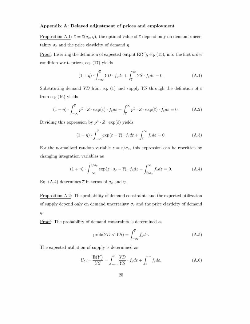
Appendix A: Delayed adjustment of prices and employment

Proposition A.1: ε = ε(σε, η), the optimal value of ε depend only on demand uncer-

tainty σε and the price elasticity of demand η.

Proof: Inserting the definition of expected output E(Y ), eq. (15), into the first order

condition w.r.t. prices, eq. (17) yields

(1 + η) ·

∫ ε

−∞

YD · fεdε +

∫

∞

εYS · fεdε = 0. (A.1)

Substituting demand YD from eq. (1) and supply YS through the definition of ε

from eq. (16) yields

(1 + η) ·

∫ ε

−∞

pη · Z · exp(ε) · fεdε +

∫

∞

εpη · Z · exp(ε) · fεdε = 0. (A.2)

Dividing this expression by pη · Z · exp(ε) yields

(1 + η) ·

∫ ε

−∞

exp(ε − ε) · fεdε +

∫

∞

εfεdε = 0. (A.3)

For the normalized random variable z = ε/σε, this expression can be rewritten by

changing integration variables as

(1 + η) ·

∫ ε/σε

−∞

exp(z · σε − ε) · fzdz +

∫

∞

ε/σε

fzdz = 0. (A.4)

Eq. (A.4) determines ε in terms of σε and η.

Proposition A.2: The probability of demand constraints and the expected utilization

of supply depend only on demand uncertainty σε and the price elasticity of demand

η.

Proof: The probability of demand constraints is determined as

prob(YD < YS) =

∫ ε

−∞

fεdε. (A.5)

The expected utiliation of supply is determined as

Ul :=E(Y )

YS=

∫ ε

−∞

YD

YS· fεdε +

∫

∞

εfεdε. (A.6)

25

Substituting demand YD from eq. (1) and supply YS through the definition of ε

from eq. (16) yields

Ul :=E(Y )

YS=

∫ ε

−∞

exp(ε − ε) · fεdε +

∫

∞

εfεdε. (A.7)

Since ε depends only on σε and η, prob(YD < YS) and Ul also depend only on σε

and η.

Proposition A.3: In case of sufficient capacities, the optimal price is determined

by unit labour costs, the price elasticity of demand and the expected utilization of

employment, p(w) = w/[Ul · πl · (1 + 1/η)].

Proof: Inserting the first order condition with respect to prices, eq. (A.3), for the

first integral in eq. (A.7) above yields

Ul =1 − prob(YD < YS)

(1 + 1/η), (A.8)

i.e. the expected utilization of supply can be determined from the probability of

demand constraints and the price elasticity of demand. Inserting eq. (A.8) into eq.

(23) yields eq. (24) in the main text.

Appendix B: Delayed adjustment of capacities

Proposition B.1: ε = ε(σε, η, cπk

πl

w ), the optimal value of ε depend only on demand

uncertainty σε, the price elasticity of demand η and relative unit factor costs cπk

πl

w

Proof: From eqs. (5), (8) and (9) follows

p(YC) = p(w) · exp[(ε − ε)/η] and p(w) =w

πl/(1 + 1/η). (B.1)

Inserting these expressions into the first order condition, eq. (27), yields

∫

∞

ε(exp[(ε − ε)/η] − 1) · fεdε −

c

πk

πl

w= 0. (B.2)

For the normalized random variable z = ε/σε, this expression can be rewritten by

changing integration variables as

∫

∞

ε/σε

{exp[(ε − z · σε)/η] − 1} · fzdz =c

πk

πl

w. (B.3)

26

Eq. (B.3) determines ε in terms of σε, η and cπk

πl

w .

Proposition B.2: ε and σε determine the probability capacity constraints and the

expected utilization of capacities Uc.

Proof: The probability of demand constraints is defined as

prob(YD < YC) =

∫ ε

−∞

fεdε. (B.4)

The expected utiliation of capacities is defined as

Uc :=E(Y )

YC=

∫ ε

−∞

YD

YC· fεdε +

∫

∞

εfεdε. (B.5)

Substituting demand YD from eq. (1) and capacities YC through the definition of ε

from eq. (9) yields

Uc =

∫ ε

−∞

exp(ε − ε) · fεdε +

∫

∞

εfεdε. (B.6)

Proposition B.3: E(p) = (w/πl + c/πk)/(1 + 1/η), the expected price is determined

as mark-up over unit factor costs.

Proof: The first order condition w.r.t. the capital stock, eq. (27), can be rewritten

as∫

∞

εp(YC) · fεdε =

∫

∞

εp(w) · fεdε +

c

πk/(1 + 1/η) = 0. (B.7)

Expected prices are defined as

E(p) =

∫ ε

−∞

p(w) · fεdε +

∫

∞

εp(YC) · fεdε (B.8)

Inserting eq. (B.7) for the second integral yields the requested result.

Proposition B4: The average price is determined as a mark-up over corrected factor

costs.

Proof: Expected sales are determined as

E(p · Y ) =

∫ ε

−∞

p(w) · Y (w) · fεdε +

∫

∞

εp(YC) · YC · fεdε. (B.9)

27

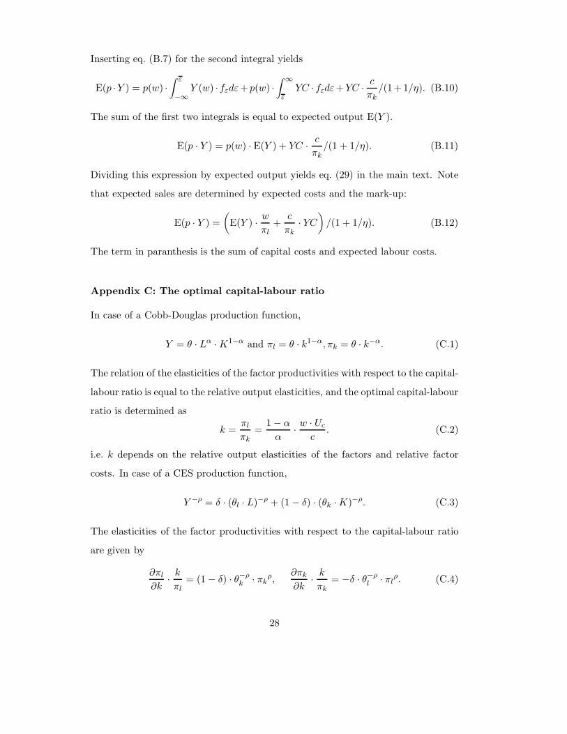
Inserting eq. (B.7) for the second integral yields

E(p ·Y ) = p(w) ·

∫ ε

−∞

Y (w) · fεdε+ p(w) ·

∫

∞

εYC · fεdε+YC ·

c

πk/(1+1/η). (B.10)

The sum of the first two integrals is equal to expected output E(Y ).

E(p · Y ) = p(w) · E(Y ) + YC ·c

πk/(1 + 1/η). (B.11)

Dividing this expression by expected output yields eq. (29) in the main text. Note

that expected sales are determined by expected costs and the mark-up:

E(p · Y ) =

(

E(Y ) ·w

πl+

c

πk· YC

)

/(1 + 1/η). (B.12)

The term in paranthesis is the sum of capital costs and expected labour costs.

Appendix C: The optimal capital-labour ratio

In case of a Cobb-Douglas production function,

Y = θ · Lα · K1−α and πl = θ · k1−α, πk = θ · k−α. (C.1)

The relation of the elasticities of the factor productivities with respect to the capital-

labour ratio is equal to the relative output elasticities, and the optimal capital-labour

ratio is determined as

k =πl

πk=

1 − α

α·w · Uc

c. (C.2)

i.e. k depends on the relative output elasticities of the factors and relative factor

costs. In case of a CES production function,

Y −ρ = δ · (θl · L)−ρ + (1 − δ) · (θk · K)−ρ. (C.3)

The elasticities of the factor productivities with respect to the capital-labour ratio

are given by

∂πl

∂k·

k

πl= (1 − δ) · θ−ρ

k · πkρ,

∂πk

∂k·

k

πk= −δ · θ−ρ

l · πlρ. (C.4)

28

ρ is the substitution parameter, δ is the distribution parameter and θl, θk are the

efficiencies of labour and capital. Inserting these expressions into the first order

condition with respect to the capital-labour ratio, eq. (32) in the main text, yields

w · Uc

c·πk

πl=

δ · θ−ρl · πl

ρ

(1 − δ) · θ−ρk · πk

ρ, (C.5)

and the optimal capital-labour ratio is determined as

k =πl

πk=

(

w · Uc

c

)1/(1+ρ)

·

(

δ

1 − δ

)1/(1+ρ)

·

(

θl

θk

)

−ρ/(1+ρ)

. (C.6)

ρ = 1/σ − 1 and σ is the elasticity of substitution.

Appendix D: A three-step decision structure

The proofs of this model correspond largely to those above in appendix B.

Proposition D.1: z = z(σz, η, cπk

πl

w ), the optimal value of z depend only on uncer-

tainty about z, the price elasticity of demand η and relative unit factor costs cπk

πl

w

Proof: From eqs. (22), (24) and (33) follows

p(YC) = p(w) · exp[(z − z)/η] and p(w) =w

πl · Ul/(1 + 1/η). (D.1)

Inserting these expressions into the first order condition, eq. (36), yields

∫

∞

z(exp[(z − z)/η] − 1) · fzdz −

c

πk

πl

w= 0. (D.2)

Rewriting eq. (D.2) for the normalized random variable z/σz yields an expression

which determines z in terms of σz, η and cπk

πl

w .

Proposition D.2: z and σz determine the probabilities of capacity constraints for

employment.

Proof: The probability of capacity constraints for employment is defined as

prob(YC < YL(w)) =

∫

∞

zfzdz. (D.3)

29

Proposition D.3: The expected utilization of capacities Uc is determined by z, σz

and the expected utilization of employment Ul.

Proof: The expected utiliation of capacities is defined as

Uc :=E(Y )

YC=

(

∫ z

−∞

YL(w)

YC· fzdz +

∫

∞

zfzdz

)

· Ul. (D.4)

Substituting YL(w) from eq. (25) and capacities YC through the definition of z from

eq. (33) yields

Uc =

(

∫ z

−∞

exp(z − z) · fzdz +

∫

∞

zfzdz

)

· Ul. (D.5)

Proposition D.4: E(p) = (w/πl + c/πk)/(1 + 1/η), the expected price is determined

as mark-up over unit factor costs.

Proof: The first order condition w.r.t. the capital stock, eq. (36), can be rewritten

as∫

∞

zp(YC) · fzdz =

∫

∞

zp(w) · fzdz +

c

Ul · πk/(1 + 1/η) = 0. (D.6)

Expected prices are defined as

E(p) =

∫ z

−∞

p(w) · fzdz +

∫

∞

zp(YC) · fzdz (D.7)

Inserting the first order condition for the second integral and p(w) from eq. (24)

yields the requested result.

Proposition D.5: The average price is determined as mark-up over corrected factor

costs.

Proof: Expected sales are determined as

E(p · Y ) =

(

∫ z

−∞

p(w) · YL(w) · fzdz +

∫

∞

zp(YC) · YC · fzdz

)

· Ul. (D.8)

Inserting the first order condition for the second integral yields, substituting ex-

pected output E(Y ) and dividing by expected output yields eq. (38) in the main

text (see appendix B, proposition B.4 above).

30