Cournot outcomes under Bertrand-Edgeworthcompetition with demand uncertainty

Jason J. Lepore�y

November 25, 2011

Abstract

We provide new results for two-stage games in which �rms make capacity invest-ments when demand is uncertain, then, when demand is realized, compete in prices.We consider games with demand rationing schemes ranging from e¢ cient to propor-tional rationing. In all cases, there is a subgame perfect equilibrium outcome coincidingwith the outcome of the Cournot game with demand uncertainty if and only if (i) the�uctuation in absolute market size is small relative to the cost of capacity, or (ii) un-certainty is such that with high probability the market demand is very large and withthe remaining probability the market demand is extremely small. Otherwise, equilibriainvolve mixed strategies. Further, we show under e¢ cient rationing that condition (i)is su¢ cient for the unique equilibrium outcome to be an equilibrium outcome of theCournot game with demand uncertainty.Keywords Bertrand-Edgeworth duopoly; Demand rationing; Cournot duopoly;

Demand uncertaintyJEL Classi�cations D21 � D43 � L11 � L13

�I would like to thank Massi DeSantis, Wei-Min Hu, Chris Knittel, Klaus Nehring, Burkhard Schipperand Aric Shafran for their helpful comments. I would like to particularly thank Louis Makowski and JoaquimSilvestre for helping with the development of this manuscript.

yAddress: Department of Economics, Orfalea Business College, California Polytechnic State Univer-sity, San Luis Obispo, CA 93407; e-mail : jlepore@calpoly.edu; phone: (805) 756-1618; web: www.econ-jasonlepore.com.

1

2

1 Introduction

We analyze competition between �rms that must invest in capacity before demand is known.After these capacity investments are sunk, demand is realized and competition commencesin prices. The goal of this paper is to understand when capacity investment decisions in sucha scenario can be modeled by using market clearing prices à la Cournot. That is, we aimto understand the general conditions under which the conclusion of Kreps and Scheinkman(1983) (hereafter K&S) holds with uncertain demand.1

Two previous papers have analyzed closely related two-stage games.2 As a preliminarystep in the analysis of collusive equilibria of a repeated game, Staiger and Wolak (1992) studya two-stage game with linear demand, continuously distributed uncertainty and e¢ cientrationing. They make the incorrect claim that a unique pure symmetric capacity subgameperfect equilibrium always exists.3 This error was pointed out by Reynolds and Wilson(2000) (hereafter R&W) who generalize the two-stage game by allowing a more generalclass of concave demand functions. R&W�s primary theorem gives necessary and su¢ cientconditions for the uncertain Cournot outcome to be an equilibrium outcome of the two-stagegame. A very interesting insight from R&W is that their model often involves asymmetriccapacity investment and mixed strategy pricing. Our speci�cation nests the aforementionedarticles including a extremely wide range of demand uncertainty, as well as, a range of residualdemand rationing schemes from e¢ cient to proportional rationing.4 We provide more generalresults that are intuitively similar to R&W�s claims, and further, provide results pertainingto uniqueness of equilibrium.

In a preliminary step of our analysis, we characterize the equilibria of a Cournot gamewith demand uncertainty. The Cournot game with demand uncertainty may possess many

1There is a signi�cant literature, not directly related to our purpose, taking the analysis of the two-stage games in many interesting directions. Some examples are: Deneckere and Kovenock (1992) (Capacityconstrained with sequential pricing); Allen (1993) and Allen et al. (2000) (sequential capacity choice gamewith simultaneous pricing); Deneckere and Kovenock (1996) (asymmetric costs of production up to capacity);Maggi (1996) and Boccard and Wauthy (2000,2004) (costly adjustment of capacity in the second stage).

2In a related paper, Hviid (1991) studies Betrand-Edgeworth pricing games where demand is still uncertainwhen prices are chosen. Fabra and de Frutos (2011) also analyze a game two-stage game closely related toours. They assume demand is composed of a mass of consumers who each demand one unit if the price is lessthan or equal to one and zero otherwise. The �rms are uncertain about the mass of consumers that will beat the market. One of the special features of these rectangular demand functions is that all rationing rulesare the same and are e¢ cient. Since we only consider downward sloping demand, their game is a limitingcase of our model, just outside of our speci�cation.

3The incorrect claim is actually fairly innocuous to their primary purpose, the study of collusive pricing.For a discussion of this point see Reynolds and Wilson (2000), Section 4.

4K&S (1983) results only pertain to the case of e¢ cient rationing of residual demand. Davidson andDeneckere (1986) make a compelling argument for the use proportional rationing and show the Cournotoutcome is not always the equilibrium outcome of the two-stage game with proportional rationing. Lepore(2009) derives precise conditions when the Cournot outcome is an equilibrium of the two-stage game withproportional rationing.

3

equilibria (hereafter labeled UCE), which are all symmetric. We denote by an uncertainCournot outcome (UCO), the prices and capacities (quantities) of a UCE.5

The analysis of the two-stage game is restricted to subgame perfect equilibria and hence,we analyze a game where �rms choose only capacities and expected revenue is determinedby the Nash equilibrium of the pricing subgame. We denote this game the capacity choicegame.

Our �rst result regarding the capacity choice game is that there exists an equilibrium witha UCO if and only if with probability one, each �rm�s best response to its rival choosing thelargest uncertain Cournot capacity leads to pure strategy pricing. There are two scenarioswhere this condition is satis�ed: (i) the range of uncertainty in demand is small and the costof capacity is relatively high, or (ii) there is high probability of large demand states, lowprobability of states with very limited absolute demand and the cost of capacity is relativelylow.

A su¢ cient condition for the UCO to be the unique equilibrium outcome of the capacitychoice game is that neither �rm will ever choose to be the weakly larger �rm when mixedstrategy pricing can occur with positive probability. Under e¢ cient rationing, this conditionis satis�ed if the largest UCE capacities lead to Cournot pricing with probability one, whichis true for scenario (i) above.

After presenting the general results, we restrict uncertainty to be continuously distributedand compare our results with R&W�s. This uncovers an error in the characterization ofR&W. The characterization we �nd is slightly di¤erent than R&W�s, but similar in economiccontent. We provide additional assumptions, stronger than R&W�s, which recover theirexact characterization. Further, under e¢ cient rationing we show that if an equilibrium ofthe capacity choice game has a UCO, then it is the unique equilibrium of the capacity choicegame.

The structure of the rest of the paper goes as follows. The basic assumptions and de�n-itions of the model are outlined in Section 2. In Section 3, the set of UCE is characterized.Section 4 is a synthetic characterization of the Nash equilibria of the pricing subgames forall rationing schemes. The general results are stated in Section 5. In Section 6, we applyour general results to the special case of uncertainty following a continuous distribution, andSection 7 concludes the paper.

2 Model Basics

The model has two �rms, 1 and 2, that choose capacities denoted x and y, respectively.The parameter � is the market demand level. It is a random variable with a particular

5Throughout the paper the term capacity and quantity will be used as synonyms.

4

distribution � on the compact space � � Rn+. The market inverse demand is the functionP (q; �) : R2+ 7! R+ and the market demand is the function D(p; �) : R2+ 7! R+. We statethe formal assumptions:

Assumption 1 For each � 2 �; there exists a quantity X(�) such that 8q 2 [0; X(�)),P (q; �) 2 (0;1) and 8q � X(�), P (q; �) = 0. On (0; X(�)), P (q; �) is twice-continuouslydi¤erentiable, strictly decreasing and concave in q.

Assumption 2 For all �; �0 2 � such that � 6= �0, there exists q 2 R+ such that P (q; �) 6=P (q; �0).

The second assumption imposes minimal restriction on the nature of demand uncertainty.For the set of parameters �, inverse demand functions are allowed to cross, become moreor less concave, and move discontinuously in the parameter �. For notational convenience,we will often write the partial derivative with respect to the �rst argument as @qP (x; �) =@P (q; �)=@qjq=x.

Assumption 3 Both �rms face the same capacity cost function a : R+ 7! R+, which istwice-continuously di¤erentiable, nondecreasing, convex, and satis�es a(0) = 0. The costfunction is such that 0 < a0(0) < E [@qP (0; �) + P (0; �)].

De�ne �X = maxX(�). For each state inverse demand function, as q goes toward theupper bound X(�), we assume the derivative of the inverse demand is bounded.

Assumption 4 For all � 2 �, there exists a �nite (�) 2 R+ such that��limx"X(�) @qP (x; �)�� � (�).

The two-stage game has the following timing. At the beginning of the game, the demandparameter � is uncertain and each �rm simultaneously and independently chooses its capacitylevel. Both �rms observe the realized demand parameter � and the other �rm�s capacity,then choose simultaneously and independently their prices.

We restrict the analysis of the two-stage game to subgame perfect equilibria. Hence, westudy a capacity choice game where expected revenues are taken as deterministic functionsof capacities. The expected revenue functions are constructed from the Nash equilibria ofthe pricing subgames.

In addition, two auxiliary games �the Cournot game and the uncertain Cournot game�are used to characterize the equilibria of the capacity choice game.

5

The �rst auxiliary game is the standard Cournot game for a given demand parameter� 2 � and zero cost. It is well known that under assumptions 1-4, given a �xed � 2 �,there exists a unique Cournot equilibrium, which is symmetric.6 Denoted by bq(�) a �rm�sequilibrium quantity (capacity).

The second auxiliary game, the uncertain Cournot game, has the following timing. Atthe beginning of the game the demand parameter � is uncertain and each �rm chooses itscapacity level independently and simultaneously. Then the demand parameter is realizedand price is determined by market clearing such that p1 = p2 = P (q1 + q2; �). Section 3 isdevoted to characterizing the equilibria of the uncertain Cournot game.

3 Uncertain Cournot Game

The purpose of this section is to establish the character of the set of UCE, which is the basisfor understanding the extension of the K&S result to demand uncertainty.

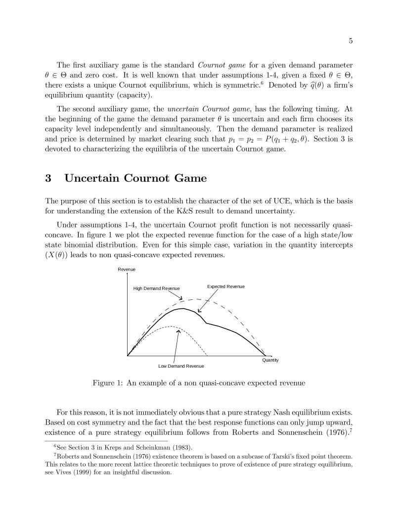
Under assumptions 1-4, the uncertain Cournot pro�t function is not necessarily quasi-concave. In �gure 1 we plot the expected revenue function for the case of a high state/lowstate binomial distribution. Even for this simple case, variation in the quantity intercepts(X(�)) leads to non quasi-concave expected revenues.

Low Demand Revenue

High Demand Revenue Expected Revenue

Revenue

Quantity

Figure 1: An example of a non quasi-concave expected revenue

For this reason, it is not immediately obvious that a pure strategy Nash equilibrium exists.Based on cost symmetry and the fact that the best response functions can only jump upward,existence of a pure strategy equilibrium follows from Roberts and Sonnenschein (1976).7

6See Section 3 in Kreps and Scheinkman (1983).7Roberts and Sonnenschein (1976) existence theorem is based on a subcase of Tarski�s �xed point theorem.

This relates to the more recent lattice theoretic techniques to prove of existence of pure strategy equilibrium,see Vives (1999) for an insightful discussion.

6

In the following theorem we prove that all pure strategy UCE quantities (capacities) aresymmetric and must satisfy a right-hand derivative condition. These two facts are extremelyuseful in the con�guration of our primary results. Denote by q� an equilibrium quantity ofthe uncertain Cournot game and denote the largest of all such symmetric UCE capacitiesby q.

In order to establish notation, the uncertain Cournot expected pro�t is

�ca(x; y) = E [P (x+ y; �)x]� a(x), (1)

and an uncertain Cournot game best response correspondence is

�ca(y) = arg maxx2[0; �X]

�c(x; y). (2)

Theorem 1 Every pure strategy UCE is symmetric and satis�es the condition

E [@qP (2q�; �)q� + P (2q�; �) j U (2q�)]� a0(q�) = 0, (CE)

where U (q) = f� 2 � j q < D(0; �)g.8

All proofs are provided in the appendix.

4 The Pricing Subgames

Before we move to the characterization of the Nash equilibria of pricing subgames, we for-mally address the way in which demand is rationed.

4.1 Rationing Schemes

More speci�cally, the demand served by �rm i is:

Dri (p1; p2; �) =

8><>:minfx;D(pi; �)g if pi < pjmin

nx;max

nD(pi;�)2; D(pi; �)� y

ooif pi = pj

min fx;max f0; dri (p1; p2; �)gg if pi > pj

; (3)

8At any q = D(0; �), the revenue function for state � is not di¤erentiable. This is apparent by the kinkin the expected revenue function of �gure 1. The right-hand derivative of the revenue function for state �must be zero at this point. Thus, our restriction to the set U(2q) removes these non-di¤erentiable pointsfrom the expression; giving the right-hand derivative at q.

7

where r 2 fe; pg, �e�represents �e¢ cient rationing�and �p�represents �proportional ra-tioning.� The residual demand dri (p1; p2; �) is the only term that varies with r. The tworesidual demands for r = e and r = p are:

dei (pi; pj; �) = D(pi; �)� y,and

dpi (pi; pj; �) = D(pi; �)

�1� y

D(pj; �)

�.

It is also necessary to de�ne a series of demand rationing schemes that are betweene¢ cient and proportional rationing. The set of rationing schemes � is such that, for all(p1; p2), dri (p1; p2; �) 2 [D(pi; �) � y;D(pi; �)(1 � y=D(pj; �))] and dri (p1; p2; �) is continuousand weakly decreasing in both the prices.

In what follows, we will specify results that pertain to the all rationing schemes �, asopposed to results that pertain to a particular scheme.

4.2 Equilibria of Pricing Subgames

There is a pricing subgame for each � 2 �. Here we �x the two �rms�capacity choices atarbitrary values x and y and examine the pricing subgame given any demand realization.

We denote equilibrium mixed strategies of the pricing subgame of demand parameter �by (�r1;�

r2).

9 The characterization below follows from the characterization shown in Lepore(2009), which is based on results from K&S, Davidson and Deneckere (1986) and Deneckereand Kovenock (1992). In order to delineate pricing regions, we de�ne the Cournot bestresponse function for demand parameter � for a �rm with zero cost

r(y; �) = argmaxx2[0;X(�)] P (x+ y; �)x.

Denote by xm(�) and pm(�), the zero cost monopoly capacity (quantity) and price, respec-tively, for demand parameter �.

It is useful to classify the three regions of equilibrium pricing based on the demandparameter �. For either rationing rule, the unique equilibrium is cut-throat Bertrand pricingfor parameter � if minfx; yg � X(�). Formally, the set of Bertrand pricing parameters, forany x and y, is

B(x; y) = f� 2 � j minfx; yg � X(�)g .

The region of Cournot pricing depends on the rationing rule. The set of demand parameterswith Cournot pricing under proportional rationing is Cp(x; y), under e¢ cient rationing it is

9Existence of mixed strategy Nash equilibria in the capacity constrained pricing games is based on resultsin Dasgupta and Maskin (1986a&b) and Maskin (1986).

8

Ce(x; y). Formally,

Cp(x; y) = f� 2 � j x+ y � xm(�)g ,Ce(x; y) = f� 2 � j x � r(y; �) and y � r(x; �)g .

Notice that Cp(x; y) � Ce(x; y).

For all rationing schemes r 2 �, the set of capacities such that the subgame equilibriumhas Cournot pricing is Cr(x; y). The set Cr(x; y) is nonempty and Cp(x; y) � Cr(x; y) �Ce(x; y). The following lemma establishes this formally.

Lemma 1 For all r 2 �, Cr(x; y) � Ce(x; y) and Cp(x; y) � Cr(x; y).

Under any rule r 2 �, for any other capacity combinations the existence of equilibriais only guaranteed in mixed strategy pricing. We de�ne the mixed strategy pricing regionsbelow.

M ri (x; y) = f� 2 � j � =2 Cr(x; y), y < X(�) and x � yg ;

mri (x; y) = f� 2 � j � =2 Cr(x; y), x < X(�) and x < yg :

De�ne Mr(x; y) = mri (x; y) [M r

i (x; y), the set of all mixed capacities for the parameter �.

We now focus on a characterization of the equilibrium expected revenue the cases r 2fe; pg. We can be more speci�c about the the Nash equilibrium expected revenue of �rm i

is for the cases r 2 fe; pg,

Rr(x; y; �) =

8>><>>:P (x+ y; �)x if � 2 Cr(x; y)�r(y; �) if � 2M r

i (x; y)

pr(x; y; �)x if � 2mri (x; y)

0 if � 2 B(x; y),

where,

�e(y; �) = P (r(y; �) + y; �)r(y; �),

�p(y; �) = pm(�)xm(�)

Z pm(�)

P (y;�)

�1� y

D(z;�)

�d�p2(z):

The term pr(x; y; �) is the lowest price in the support of equilibrium pricing, it is a piecewisefunction de�ned in what follows. If � 2 Mr(x; y), then the expected revenue of each �rm isdetermined by the lowest price in the support of mixed strategy of the smaller �rms. Thereare two possible lowest prices of the support. First

�r(x; y; �) = min fp 2 R+ j py = �r(x; �)g . (4)

9

The function �r is de�ned 8y > 0 8x � 0, and is twice-continuously di¤erentiable 8x 2�0; �X

�. The second possible price applies when the opposing �rm is larger,

�r(x; �) = min fp 2 R+ j pD(p; �) = �r(x; �)g . (5)

The function �r is de�ned 8x � 0, and is twice-continuously di¤erentiable 8x 2�0; �X

�. The

actual price is the maximum of the two prices in (4) and (5)

pr(x; y; �) = max f�r(x; y; �); �r(x; �)g . (6)

For the cases r 2 fe; pg, the capacity choice expected pro�t given Nash equilibrium pricingis de�ned as

�ra(x; y) = E [Rr(x; y; �)]� a(x).

Denote the capacity choice best response by

�ra(y) 2 arg maxx2[0; �X]

�ra(x; y).

Note that, for r 2 fe; pg, the function �ra(x; y) is bounded and continuous for all (x; y) 2 R2+.Hence, for any y 2 [0; �X], it attains a maximum on x 2 [0; �X]: A continuous function on acompact rectangle in R2+ is uniformly continuous on that rectangle; and, in turn, a uniformlycontinuous function on a compact space has a closed set of maximizers. Thus, the set �ra(y)is closed for all y 2 [0; �X] i.e., for all y 2 [0; �X] and for any sequence hyni that converges toy, we have that limn!1 �

ra(y

n) 2 �ra(y).

For the general case of r 2 �, it is not clear that a unique equilibrium expected revenueexists for each pair of capacities (x; y) 2 Mr(x; y). We de�ne some additional notation tohelp understand the expected revenue of all equilibria for all r 2 �.

Denote the index �(�) for an arbitrary equilibrium expected revenueRr(x; y; � : �(x; y; �)),given capacities (x; y) and the state �. The set of all indexes for di¤erent equilibria given(x; y) and the state � is denoted by A(x; y; �). Denote a possible expected pro�t of �rm a by�ra(x; y : �) = E [R

r(x; y; � : �(x; �))] � a(x) for all � 2 A(y) =Qx2[0; �X]

�Q�2�A(x; y; �)

�.

Denote the best response given a certain set of equilibrium expected revenues of the pricingsubgame � 2 A(y),

�ra(y : �) 2 arg maxx2[0; �X]

�ra(x; y : �):

Finally, de�ne the set of all possible best responses to y, for all � 2 A(y),

Bra(y) =[

�2A(y)�ra(y : �).

In the following preliminary result, we establish that for any rationing r 2 � all subgameperfect equilibrium expected pro�t are weakly greater than the expected subgame perfect

10

equilibrium expected pro�t with e¢ cient rationing.

Lemma 2 For all r 2 �, �ra(x; y : �) � �ea(x; y) for all (x; y) 2 [0; �X]�[0; �X] and � 2 A(y).

5 The Capacity Choice Game

We �rst show the necessary and su¢ cient conditions for a UCO to be an equilibrium outcomeof the capacity choice game. Then we provide a su¢ cient condition for the unique purestrategy equilibria of each capacity choice game to have a UCO.10

5.1 Existence

Regardless of rationing rule, a variation of the same condition de�nes the existence of equi-librium with a UCO. There is a capacity choice equilibria with a UCO if and only if thereis a best response to q that is not both, larger than q and leads to mixed strategy pricingwith positive probability. It also turns out that only the largest capacity UCO can be anequilibrium of the capacity choice game. These facts are formalized in the theorem below.

Theorem 2 Consider the capacity choice game de�ned above by assumptions 1� 4.

1. For any rationing rule r 2 �, the only equilibrium of the capacity choice game that canhave a UCO is x = y = q. Further, if rationing is e¢ cient, then x = y = q are theonly symmetric capacities that can be an equilibrium.

2. For any rationing rule r 2 �, the UCE capacities, x = y = q; are an equilibrium of thecapacity choice game if and only if

9x 2 Bra(q)such that � (Mr(x; q)) = 0. (7)

We provide an example to give some basic context to statements of the theorem. Inthe example, Condition 7 is violated and there is no equilibrium with the UCO. After theexample, we move to a sketch of the proof of Theorem 2.

Example 1 (No UCO) This example is constructed to show that when Condition 7 is notsatis�ed, q is not an equilibrium. Assume that demand is rationed according to the e¢ cientrationing rule. De�ne the inverse demand function P (q; �) = maxf��q; 0g where � 2 f8; 18g.10As a side note, an equilibrium of the capacity choice game in mixed strategies always exists. Existence

follows immediately form Glicksberg (1952) since the pro�t functions are continuous in both �rms capacities.

11

The probability that � = 8 is �(8) = 1=2 and that � = 18 is �(18) = 1=2. The marginal costof capacity is the constant 1. The unique UCE is the symmetric capacity q = 4. The capacitychoice game best response of �rm 1 to �rm 2 playing y = 4 is the capacity x = 6. Thus,x = y = 4 is not an equilibrium of the capacity choice game. For the demand state � = 8the capacities (6; 4) result in mixed strategy pricing (this is because r(4; � = 8) = 2 < 6 andminf4; 6g < X(� = 8) = 8). Therefore �(Me(6; 4)) = 1=2 > 0, a violation of Condition 7.We plot the �rms�best response correspondences in Figure 2. Notice that the discontinuity inthe best response correspondences prevents the crossing at any symmetric capacities. Thereare two asymmetric pure capacity equilibrium with one �rm playing 4:86 and the other playing5:57. In demand state � = 18, equilibrium pricing is market clearing: p1 = p2 = 7:57, whilein demand state � = 8, equilibrium pricing is in mixed strategies.

Figure 2: The best response correspondence of �rms when Condition 7 is violated.

The outline of the proof of Theorem 2 goes as follows. We begin the proof of part 1addressing only the e¢ cient rationing case and establishing two preliminary lemmas. In the�rst lemma, we establish that there can only be one symmetric pure capacity equilibrium,labeled the candidate. Recall Theorem 1, which shows that all UCE must be symmetric.Thus, only if the candidate is an equilibrium, can the outcome of an equilibrium of thetwo-stage game coincide with that of an analogue uncertain Cournot equilibrium.

The candidate corresponds with the pure symmetric capacity that Staiger and Wolak(1992) claim is always an equilibrium. We show that the candidate is uniquely de�ned bythe right-hand derivative of the expected pro�t function of each �rm equating to zero. Wedenote by bx the candidate capacity, which is de�ned by the equality

E [@qP (2bx; �)bx+ P (2bx; �) j Ce(bx; bx)]� a0(bx) = 0: (SC)

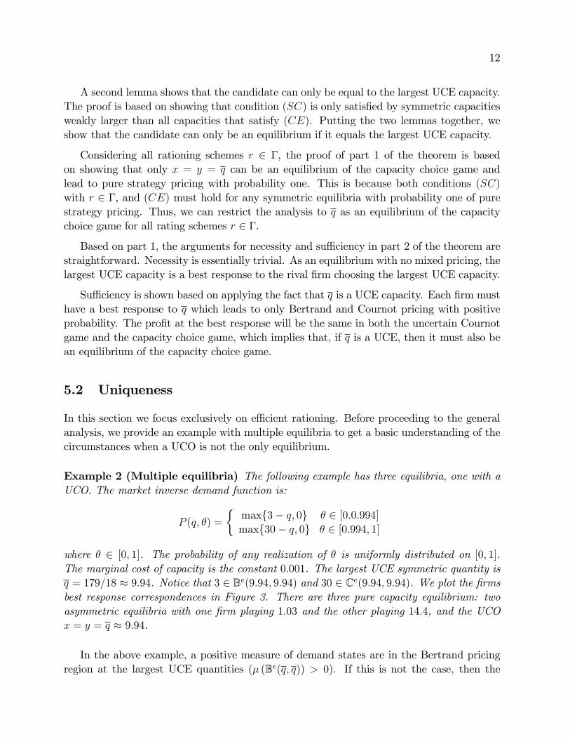
12

A second lemma shows that the candidate can only be equal to the largest UCE capacity.The proof is based on showing that condition (SC) is only satis�ed by symmetric capacitiesweakly larger than all capacities that satisfy (CE). Putting the two lemmas together, weshow that the candidate can only be an equilibrium if it equals the largest UCE capacity.

Considering all rationing schemes r 2 �, the proof of part 1 of the theorem is basedon showing that only x = y = q can be an equilibrium of the capacity choice game andlead to pure strategy pricing with probability one. This is because both conditions (SC)with r 2 �, and (CE) must hold for any symmetric equilibria with probability one of purestrategy pricing. Thus, we can restrict the analysis to q as an equilibrium of the capacitychoice game for all rating schemes r 2 �.

Based on part 1, the arguments for necessity and su¢ ciency in part 2 of the theorem arestraightforward. Necessity is essentially trivial. As an equilibrium with no mixed pricing, thelargest UCE capacity is a best response to the rival �rm choosing the largest UCE capacity.

Su¢ ciency is shown based on applying the fact that q is a UCE capacity. Each �rm musthave a best response to q which leads to only Bertrand and Cournot pricing with positiveprobability. The pro�t at the best response will be the same in both the uncertain Cournotgame and the capacity choice game, which implies that, if q is a UCE, then it must also bean equilibrium of the capacity choice game.

5.2 Uniqueness

In this section we focus exclusively on e¢ cient rationing. Before proceeding to the generalanalysis, we provide an example with multiple equilibria to get a basic understanding of thecircumstances when a UCO is not the only equilibrium.

Example 2 (Multiple equilibria) The following example has three equilibria, one with aUCO. The market inverse demand function is:

P (q; �) =

�maxf3� q; 0g � 2 [0:0:994]maxf30� q; 0g � 2 [0:994; 1]

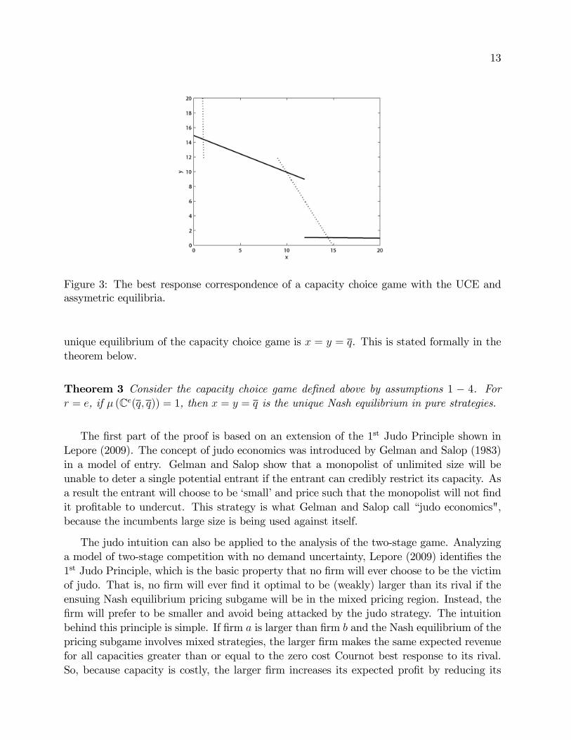
where � 2 [0; 1]. The probability of any realization of � is uniformly distributed on [0; 1].The marginal cost of capacity is the constant 0:001. The largest UCE symmetric quantity isq = 179=18 � 9:94. Notice that 3 2 Be(9:94; 9:94) and 30 2 Ce(9:94; 9:94). We plot the �rmsbest response correspondences in Figure 3. There are three pure capacity equilibrium: twoasymmetric equilibria with one �rm playing 1:03 and the other playing 14:4, and the UCOx = y = q � 9:94.

In the above example, a positive measure of demand states are in the Bertrand pricingregion at the largest UCE quantities (� (Be(q; q)) > 0). If this is not the case, then the

13

Figure 3: The best response correspondence of a capacity choice game with the UCE andassymetric equilibria.

unique equilibrium of the capacity choice game is x = y = q. This is stated formally in thetheorem below.

Theorem 3 Consider the capacity choice game de�ned above by assumptions 1 � 4. Forr = e, if � (Ce(q; q)) = 1, then x = y = q is the unique Nash equilibrium in pure strategies.

The �rst part of the proof is based on an extension of the 1st Judo Principle shown inLepore (2009). The concept of judo economics was introduced by Gelman and Salop (1983)in a model of entry. Gelman and Salop show that a monopolist of unlimited size will beunable to deter a single potential entrant if the entrant can credibly restrict its capacity. Asa result the entrant will choose to be �small�and price such that the monopolist will not �ndit pro�table to undercut. This strategy is what Gelman and Salop call �judo economics",because the incumbents large size is being used against itself.

The judo intuition can also be applied to the analysis of the two-stage game. Analyzinga model of two-stage competition with no demand uncertainty, Lepore (2009) identi�es the1st Judo Principle, which is the basic property that no �rm will ever choose to be the victimof judo. That is, no �rm will ever �nd it optimal to be (weakly) larger than its rival if theensuing Nash equilibrium pricing subgame will be in the mixed pricing region. Instead, the�rm will prefer to be smaller and avoid being attacked by the judo strategy. The intuitionbehind this principle is simple. If �rm a is larger than �rm b and the Nash equilibrium of thepricing subgame involves mixed strategies, the larger �rm makes the same expected revenuefor all capacities greater than or equal to the zero cost Cournot best response to its rival.So, because capacity is costly, the larger �rm increases its expected pro�t by reducing its

14

capacity to exactly the zero cost Cournot best response to its rival, which moves the pricingsubgame from the mixed strategy region to into the pure strategy market clearing pricingregion.

In the uncertain demand model with e¢ cient rationing the extension of 1st Judo principleis: Given that the largest UCE capacities lead to non-zero market clearing prices withprobability 1, no �rm will ever choose to have be the victim of judo with positive probability.We can restate this result more formally as: � (Ce(q; q)) = 1, which implies that no �rm willever want to be the weakly larger �rms when there is positive probability that the pricing isin mixed strategies.

The rest of the proof goes as follows. The condition � (Ce(q; q)) = 1 implies that (7) holdsat x = y = q. Hence, based on Theorem 1, x = y = q is a Nash equilibrium of the capacitychoice game. There cannot be an equilibrium with positive probability of mixed strategies,because one �rm must be weakly larger with positive probability. Thus, equilibria can onlybe such that Cournot and Bertrand pricing are probable outcomes. The only equilibriumof this form is x = y = q. Therefore, x = y = q is the unique Nash equilibrium in purestrategies of the capacity choice game.

In the following section we restrict the model to get a more intuitive characterization andcompare the results to R&W.

6 A Restricted Characterization

In this section we provide special characterizations with more restricted assumptions. Thistreatment is closely related to the analysis done in R&W. R&W assume the distributionof uncertainty is continuous with full support on the parameter space and that demandis rationed using the e¢ cient rule.11 In R&W�s Theorem 1 they claim that with e¢ cientrationing, x = y = q� is a Nash equilibrium of the capacity choice game if and only ifbq(�) � q�. It turns out this condition does not characterize x = y = q� as a Nash equilibriumof the capacity choice game. In Section 3 we hinted at the fact that multiple UCE canexist under our assumptions. The assumptions of R&W do not preclude this possibility.This provides an immediate problem with their result (since q� is not well de�ned). Evenwhen the UCE is unique, the conditions of R&W are neither necessary nor su¢ cient. Inthe following example, with a unique UCE, we show that the conditions of R&W are notnecessary for the existence of a UCO.

Example 3 (Counter example to R&W ) Let us reconsider a slightly di¤erent version

11R&W also assume that marginal cost is constant and a larger demand state indexes a larger inversedemand for all �xed quantities: � = [�; �], and for all �; �0 2 [�; �] such that � > �0, P (q; �) > P (q; �0) for allq 2 R+.

15

of Example 2, which �ts the assumption of R&W. De�ne the market inverse demand:

P (q; �) =

�maxf3 + �� � q; 0g � 2 [0:0:994]maxf30 + �� � q; 0g � 2 [0:994; 1] ;

where � = 1� 10�200. Since � = 0, bq(0) = 1=3 and the unique UCE of the game is q� � 9:94.Just as in example 2, x = y = q� � 9:94 is an equilibrium of the capacity choice game. Butthe condition of R&W that bq(�) � q� is clearly violated since bq(0) = 1=3 < 9:94 = q�.In what follows, we add assumptions and incrementally arrive at more restrictive char-

acterizations. With three additional assumptions, we are able to recover exactly R&W�scharacterization. Further, we show on this restricted domain that R&W�s conditions alsocharacterize uniqueness of equilibrium.

Let us begin with a restriction that the inverse demand is continuous in the uncertaintyparameter and the distribution of uncertainty has full support on a compact interval ofvalues.

Assumption 5 8q 2 (0; X(�)), P (q; �) is continuous in � on [�; �], and that � is positivewith continuous support on [�; �], where 0 � � < � <1.

R&W assume the distribution of uncertainty is continuous with full support on the para-meter space. We have added the assumption that the inverse demand changes continuously inthe demand parameter. With this assumption we get a characterization for e¢ cient rationingwith a similar �avor to R&W�s. Further, our characterization is stronger as it provides anecessary and su¢ cient condition for the Cournot outcome to be the unique pure strategyequilibrium outcome under e¢ cient rationing.

Corollary 1 Under assumptions 1-5:

For r = e :

(e.1) If min bq(�) � _q, then x = y =

_q is the unique Nash equilibrium in pure strategies.

(e.2) If min bq(�) < _q, then x = y = q is not a Nash equilibrium.

For r = p :

(p.1) If minxm(�) �_q, then x = y =

_q is a Nash equilibrium in pure strategies.

(p.2) If minxm(�) <_q, then x = y = q is not a Nash equilibrium.

16

Based on Assumption 5, min bq(�) � q and min bq(�) < q imply � (M ei (q; q)) = 0 and

� (M ei (q; q)) > 0, respectively. Hence, the proof of existence is an immediate consequence of

Theorem 2, while uniqueness is an immediate consequence of Theorem 3.

To recover the exact characterization of R&W we must add two more assumptions. Theaddition of the following condition on the inverse demand and nature of uncertainty issu¢ cient to guarantee a unique UCE.

Assumption 6 8q 2 (0; X(�)), P (q; �) and � are continuously di¤erentiable in � on [�; �].

Proposition 1 Under assumptions 1-6, the uncertain Cournot game has a unique equilib-rium.

To recover the exact characterization of R&W we add the �nal assumption.

Assumption 7 8(�; �0) 2 [�; �]� [�; �] and 8q 2 (0; X(�)), @qP (q; �0) � @qP (q; �) if �0 > �.

As shown in Proposition 1, the addition of Assumption 6 guarantees uniqueness of UCE.While, Assumption 7 ensures that min bq(�) = bq(�). Hence, the two conditions min bq(�) � qand min bq(�) < q can be re-written as bq(�) � q� and bq(�) < q�, respectively. This leads tothe following result where R&W�s conditions are necessary and su¢ cient for the existenceof the UCO in the capacity choice game. Based on our new results, the condition for theexistence of a UCO is also necessary and su¢ cient for the UCO to be the unique equilibriumoutcome of the capacity choice game.

Corollary 2 Under assumptions 1-7 and for r = e:

1. If bq(�) � q�, then x = y = q� is the unique Nash equilibrium in pure strategies.

2. If bq(�) < q�, then x = y = q� is not a Nash equilibrium.7 Conclusion

We have characterized the conditions under which a UCE outcome is an equilibrium out-come of a fairly general class of two-stage games with a broad class of rationing schemesranging from e¢ cient to proportional rationing. Further, we have shown that under e¢ cientrationing the condition for existence of a UCO is also necessary and su¢ cient for uniquenessof equilibrium. Thus, we can say that the K&S result is robust to demand uncertainty, if therange of demand uncertainty about the number of the quantity demanded is low or the mar-ginal cost of capacity is high enough. We provide a context for when the uncertain Cournotgame is an adequate reduced form for the two-stage capacity pricing game with demand�noise.�We leave for future research the exploration of further equilibrium character whenno uncertain Cournot outcome is an equilibrium outcome of the two-stage game.

17

8 Appendix

Proof of Theorem 1. The pro�t function �ca(qi; qj) = E [P (q1 + q2; �)qi] � a(qi), fori 6= j and i 2 f1; 2g, is not necessarily di¤erentiable at all qi in (0; �X � qj) because at eachquantityX(�)�qj the function has a kink. De�ne O = (0; �X)�[0; �X] and S = [0; �X]�[0; �X].Although the function has kinks, it is continuous on any subset of R2, and hence the pro�tfunction is bounded on any compact subset S. Therefore the right-hand and left-handderivatives exist for each state pro�t function as well as the expected pro�t function on O.The right-hand and left-hand derivatives of the state � pro�t function are certainly �nite forqi 2 (0; X(�) � qj) and qi > X(�) � qj, because it is di¤erentiable on these intervals. Atqi = X(�) � qj, the right-hand derivative in qi is zero and the left-hand derivative is �niteby Assumption 4. Therefore, the right-hand and left-hand derivatives of �ci can be passedinside the expectation (Theorem 16.8, Billingsley 1986).

We �rst need to show that the right-hand partial derivative in the �rm�s own capacitybeing equal to zero, is a necessary condition for a pure strategy equilibrium. The case wherethe right-hand derivative is positive is immediately ruled out because there is a pro�tableupward deviation arbitrarily close to the capacity for both �rms. We are left to provethat when the right-hand derivative is negative at (eq1; eq2), those capacities cannot be anequilibrium. Suppose to the contrary, that at an equilibrium, it is possible that @+x �(eqi; eqj) <0. For notational convenience denote eq = eq1 + eq2. De�ne the set of states with kinks at(eq1; eq2) as K(eq1; eq2) = f� 2 � j eq = X(�)g. For the states �rK(eq1; eq2), the state revenue isdi¤erentiable. For any � 2 K(eq1; eq2), the revenue for �rm i is zero at (eq1; eq2) and positive forall qi < eqi, and therefore the left-hand derivative of each state revenue is negative at (eq1; eq2).Putting these two facts together, the left-hand derivative of the expected pro�t function at(eq1; eq2) must be less than the right-hand derivative. Hence, there is a pro�table deviationqi < eqi.The second part of the proof addresses the necessary symmetry of all equilibria. Suppose

to the contrary that there is an equilibrium (eq1; eq2) that is not symmetric (without loss ofgenerality, assume that eq1 > eq2). Then, for i 2 f1; 2g, (CE) must hold for both �rms at(eq1; eq2). It will be useful to rewrite (CE):

eqiE [@qP (eq; �)jU (eq)] + E [P (eq; �)jU (eq)]� a0(eqi) = 0, (8)

for i 2 f1; 2g. The condition (CE) holds for both agents, which clearly implies that

@+x �ca(eq1; eq2) = @+x �ca(eq2; eq1): (9)

Since a is convex and eq1 > eq2, a0(eq1) > a0(eq2). Also, notice that the second term on the right-hand side of (8) is the same for both �rms. Based on (8) and (9) we derive the inequalitiesbelow, eq1E [@qP (eq; �)jU (eq)] � eq2E [@qP (eq; �)jU (eq)] .

18

Since E [@qP (eq; �)jU (eq)] < 0, the above equality reduces to eq1 � eq2, a contradiction.Proof of Lemma 1. Denote the region Cr(x; y), the set of � such that p1 = p2 =

P (x+ y; �) > 0 is a pure strategy equilibrium of the pricing subgame.

Part 1). Suppose that, without loss of generality, x � y. Now we argue that, for allr 2 �, when market clearing prices is an equilibrium, it is the unique equilibrium for anystates �. First we take any other pure pricing strategies p1 and p2.

Case 1). pi > P (x+y; �) and pi � pj. (1a) pi > pj : Firm j can increase its pro�t by pric-ing at minf(pi+pj)=2; P (y; �)g and get pro�t minf(pi+pj)=2; P (y; �)gy > pj minfD(pj); yg.(1b) pi = pj : Firm j can increase its pro�t by pricing at minf(pi� �); P (y; �)g and get pro�tminf(pi � �); P (y; �)gy > piD(pi)=2, which always holds for for small enough � > 0.

Case 2). pj < P (x + y; �) and pi � pj. Firm j can always increase pro�t by pricing atP (x+ y; �) and get P (x1 + x2; �)xj > pjxj.

We have just shown, that the in all demand states Cr(x; y), the unique pure strategyequilibrium is symmetric market clearing prices p1 = p2 = P (x + y; �) > 0. It remains toshow that in these demand states there are no mixed strategy equilibrium in the pricingsubgame.

Based on the preceding analysis, it is straightforward to deduce that the set of �rm 1�sbest responses to all of �rm 2�s prices is [P (x+ y; �); P (x; �)], and similarly for �rm 2, the setof all best responses is [P (x+ y; �); P (y; �)]. All prices that are part of a mixed strategy Nashequilibrium must be in theses sets. We use the fact that mixed strategy Nash equilibriumcan only involve best responses to the mixture other �rms prices. Take the arbitrary closedsets of prices S1 � [P (x+ y; �); P (x; �)] and S2 � [P (x+ y; �); P (y; �)]. Suppose there is amixed strategy Nash equilibrium with supports S1 and S2 such that S1 [ S2 6= P (x + y; �).We will show S1 and S2 cannot be the support of a mixed strategy equilibrium by wayof contradiction. Recall that, without loss of generality, we imposed that x � y. Denotep1 = maxS1 and p2 = maxS2. For all p2 2 (P (x + y; �); p2], the best response of �rm 1 isto price less than p2. This is because (p2 � �)x > p2maxfD(p2; �)=2; D(p2; �)� yg for smallenough � > 0. This must be true because x > maxfD(p2; �)=2; D(p2; �) � yg. Therefore,maxS1 < maxS2. But, for all p1 2 (P (x + y; �); p1], the best response of �rm 2 is toprice weakly less than p1. We will show that for all p2 � p1, p2min fD(p2; �)� x; yg �p1min fD(p1; �)� x; yg. The unique maximizer of p2minf(D(p2; �)� x) ; yg is P (x + y; �).Based on our assumptions p2min fD(p2; �)� x; yg is concave in p2. Putting the above factstogether, we know that p2minf(D(p2; �)� x) ; yg is weakly decreasing in p2, for all p2 >P (x+ y; �). Therefore, maxS1 � maxS2, which contradicts maxS1 < maxS2.

Part 2). First we show that Cp(x; y) � Cr(x; y). Fix (x; y) and take any state � 2Cp(x; y). This means that symmetric market clearing pricing is the unique equilibrium ofthe state � under the scheme p. Any defection to a price higher leads to lower pro�t than inthe case of proportional rationing. Therefore a �rm will not �nd a price increase defection

19

pro�t increasing under r unless it also does under p. A price decrease gives the �rm the samepro�t. Therefore, under r, a �rm will not have a pro�table defection unless it does underp. This implies that any pricing equilibrium with proportional rationing must be pricingequilibrium for all r 2 �.

Now we show that Cr(x; y) � Ce(x; y). Fix (x; y) and take any state � 2 Cr(x; y).Any defection to a price higher leads to higher pro�t than in the case of e¢ cient rationing.Therefore a �rm will not �nd a price increase pro�t increasing under e unless it also doesunder r. A price decrease gives the �rm the same pro�t. Therefore, under e, a �rm will nothave a pro�table defection unless it does under e. Therefore, Cr(x; y) � Ce(x; y).

Proof of Lemma 2. First take any (x; y) such that x � y, for all � 2 M ra(x; y), �rm

1 can always guarantee itself at least the expected revenue R(y; �) = maxfp(D(p; �) � y)g.The expected revenue of a mixed strategy equilibrium of the pricing subgame cannot resultin lower expected revenue than R(y; �), otherwise a pro�table defection exists to the pricepa = P (r(y; �) + y; �), which results in at least the expected revenue R(y; �). Notice that isexactly equal to e¢ cient rationing equilibrium expected revenue, i.e., R(y; �) = �e(y; �).

Next take any (x; y) such that x < y, for all � 2 mra(x; y), �rm 1 can always guarantee

itself at least the expected revenue pe(x; y; �)x. This is because any strategy for �rm b toprice lower than pe(x; y; �) is strictly dominated by pb = P (r(x; �)+x; �). No mixed strategyequilibrium can involve strictly dominated strategies. Hence, the expected revenue of amixed strategy equilibrium of the pricing subgame cannot result in lower expected revenuethan pe(x; y; �)x, otherwise a pro�table defection exists to the price pe(x; y; �).

Proof of Theorem 2

Part 1 The proof part 1 is constructed based on the following two lemmas.

Lemma 3 Consider the capacity choice game de�ned by assumptions 1 � 5, with r = e.There is a unique symmetric �candidate�subgame perfect equilibrium capacity bx characterizedby the right-hand derivative condition:

E [@qP (2bx; �)bx+ P (2bx; �) j Ce(bx; bx)]� a0(bx) = 0: (SC)

Proof of Lemma 3.

An analogous argument to that in Theorem 1 ensures that 8� 2 � the right-hand and left-hand derivatives of �ea(x; y) in x and R

e(x; y; �) in x exist, and are �nite on (0; �X)� [0; �X].Hence di¤erentiation can be passed inside the expectation. It is easy to show that theright-hand partial derivative of �ea(x; y) in x is the expression on the right-hand side of(SC) by applying Liebniz�s rule and including the fact that the right-hand derivative of the

20

revenue of any state not in Ce(bx; bx) is zero. The right-hand partial derivative of �ea(x; y) in xalways exists. For any x > y, the pro�t is twice-continuously di¤erentiable, so @+x �

ea(x; y) =

@x�ea(x; y). For all x > y, since the second derivative of the pro�t function is

E�@2qP (2bx; �)bx+ 2@qP (2bx; �)��Ce(bx; bx)�� a00(bx): (10)

For all �, @2qP (2bx; �)bx+ 2@qP (2bx; �) < 0 based on the facts that P is strictly decreasing andconcave. E

�@2qP (2bx; �)bx+ 2@qP (2bx; �)��Ce(bx; bx)� < 0. Further the cost function is convex,

�a00(bx) < 0. Therefore the expression (10) is negative, a su¢ cient condition for the concavityof �ea(x; y) for all x > y.

Based on these two facts, it is necessary that any pure symmetric capacity equilibriumsatisfy (11).

E [@qP (2bx; �)bx+ P (2bx; �)jCe(bx; bx)]� a0(bx) � 0: (11)

Next we establish that if (11) holds with strict inequality at x = y = bx, then bx cannotbe a capacity choice game equilibrium. We do this by showing that a negative right-handpartial derivative at bx implies that that left-hand partial derivative at bx is also negative. Anegative left-hand partial derivative at bx means there must be a pro�table local defectionfrom bx for both �rms.We break the parameters � into two sets

Me(bx; bx) [maxB(bx; bx) and �r (Me(bx; bx) [maxB(bx; bx)) :For all � 2 � r (Me(bx; bx) [maxB(bx; bx)), the state revenue is di¤erentiable at (bx; bx). Forall states � 2 Me(bx; bx) [maxB(bx; bx), the right-hand partial derivative of the state revenuefunction for both �rms is zero, while the left-hand partial derivative at (bx; bx) for both �rms isnegative. We show that left-hand partial derivative at (bx; bx) for all � 2Me(bx; bx)[maxB(bx; bx)separately for two cases (i) D(pe(bx; bx; �); �) � bx and (ii) D(pe(bx; bx; �); �) � bx.In case (i), for all � 2Me(bx; bx)[maxB(bx; bx) the left-hand derivative for each at (bx; bx)is:

@xr(bx; �)bxbx [@xP (bx+ r(bx; �); �)r(bx; �) + P (bx+ r(bx; �); �)]| {z }(�)

+r(bx; �)bx [@xP (bx+ r(bx; �); �)bx+ P (bx+ r(bx; �); �)] .

The term (�) is zero, based on the de�nition of r(bx; �) as the zero cost Cournot best responseto bx. The expression becomes:

r(bx; �)bx (@xP (bx+ r(bx; �); �)bx+ P (bx+ r(bx; �); �))| {z }(��)

< 0: (12)

21

The expression in (12) is negative because r(bx; �)=bx > 0 and (��) is negative; based on thefact that bx > r(bx; �) and P (x; �)x is strictly concave in x.Denote D = D(pe(bx; bx; �); �) + pe(bx; bx; �)@pD(pe(bx; bx; �); �). Then for case (ii) for all

� 2Me(bx; bx) [maxB(bx; bx) the left-hand derivative for each at (bx; bx)is:@xr(bx; �) � bxD� (@xP (bx+ r(bx; �); �)r(bx; �) + P (bx+ r(bx; �); �)+ r(bx;�)

D@xP (bx+ r(bx; �); �)bx+ r(bx;�)

D(pe(bx;bx;�);�)P (bx+ r(bx; �); �)< @xr(bx; �) � bxD� (�) + r(bx;�)

D(pe(bx;bx;�);�) (��)< 0.

The �rst inequality comes from the fact that

D(pe(bx; bx; �); �) + pe(bx; bx; �)@pD(pe(bx; bx; �); �) < D(pe(bx; bx; �); �),and the �nal inequality follows immediately from the fact that (�) = 0 and (��) < 0.We have now shown that the left-hand partial derivative for all states � 2 Me(bx; bx) [

maxB(bx; bx) is negative. Therefore the pro�t is di¤erentiable at (bx; bx) if � (Me(bx; bx) [maxB(bx; bx)) =0, otherwise and is left-hand partial derivative is negative at (bx; bx) :The �nal step in the proof is to show that a unique bx satis�es (SC). Suppose to the

contrary that there is qo 6= bx that is a pure symmetric equilibrium capacity. If qo > bx,then Ce(qo; qo) � Ce(bx; bx), and by the strict concavity of the the revenue function for any� 2 Ce(qo; qo) and qo > bx we have that

@qP (2qo; �)qo + P (2qo; �) < @qP (bx+ qo; �)bx+ P (bx+ qo; �)

< @qP (2bx; �)bx+ P (2bx; �).The second inequality is based on the fact that the inverse demand function is strictlydecreasing and concave in x. Hence, the marginal revenue of (qo; qo) on Ce(qo; qo) is greaterthan bx on Ce(qo; qo) and we have:

E [@qP (2qo; �)qo + P (2qo; �)jCe(qo; qo)] < E [@qP (2bx; �)bx+ P (2bx; �)jCe(qo; qo)]

� E [@qP (2bx; �)bx+ P (2bx; �)jCe(bx; bx)] .The second inequality holds because Ce(qo; qo) � Ce(bx; bx) and that for all � 2 Ce(bx; bx) thestate marginal revenue is non-negative. Putting the above inequality together with the factthat a(�) is convex contradicts the necessary condition for qo to be a pure strategy symmetricequilibrium. The argument for qo < bx follows analogouslyThe second lemma used to proof Theorem 2 establishes that only the largest Cournot

capacity can be an equilibrium of the capacity choice game..

22

Lemma 4 bx 6= q� < q.Proof of Lemma 4. Suppose to the contrary that bx = q� < q. Since q is an uncertainCournot equilibrium, the following equality must hold:

E [@qP (2q; �)q + P (2q; �) j U (2q)]� a0(q) = 0.

If we instead take the expectation over Ce(q; q), the expectation will be weakly larger becauseonly all of the positive terms remain in the expectation. Hence,

E [@qP (2q; �)q + P (2q; �) j Ce(q; q)]� a0(q) � 0. (13)

Since the P (q; �)q is strictly concave,

@qP (q + q�; �)q + P (q + q�; �) > @qP (2q; �)q + P (2q; �) (14)

for all � 2 Ce(q; q). Since (14)is true for each � 2 Ce(q; q), from (13) we know that

E [@qP (q + q�; �)q + P (q + q�; �) j Ce(q; q)]� a0(q) > 0. (15)

By de�nition of Ce, Ce(q; q) � Ce(q; q�), and since the marginal revenue for each � 2 Ce(q; q�)must be positive we know that

E [@qP (q + q�; �)q + P (q + q�; �) j Ce(q; q�)rCe(q; q)] � 0. (16)

Putting together (15) and (16) we have

E [@qP (q + q�; �)q + P (q + q�; �) j Ce(q; q�)]� a0(q) > 0. (17)

Expression (17) shows the right hand derivative at x = q > y = q� is positive. �ea(x; y) isstrictly concave for all x � y, hence the right-hand derivative at x = y = q� must be greaterthan at x = q > y = q�. This contradicts to the necessary condition (SC) for x = y = q�.

Next we prove statement 1 of Theorem 2. We do this separately for e¢ cient and propor-tional rationing.

(E¢ cient Rationing) Based on Lemma 4, only the UCE x = y = q can be an equilibriumof the e¢ cient rule capacity choice game. Further, from Lemma 3 the only possible symmetricequilibrium is x = y = bx.Now we show that only if bx = q, can the symmetric candidate be an equilibrium. Suppose

to the contrary that x = y = bx 6= q is a capacity choice equilibrium. Based on conditions(CE) and (SC), it is only possible that bx > q. This implies that at x = y = bx each �rm canincrease their uncertain Cournot pro�t by decreasing capacity. Hence, there exists z suchthat �ca(z; bx) > �ca(bx; bx). At x = y = bx all pricing is Cournot or Bertrand which implies

23

that �ea(bx; bx) = �ca(bx; bx). But �rms always earn weakly more pro�t at any �xed capacitiesin the capacity choice game than the uncertain Cournot game, �ea(z; bx) � �ca(z; bx). Puttingthe above fact together, �ea(z; bx) > �ea(bx; bx), a contradiction.(Proportional Rationing) The proof is done by showing that if any UCE other than q is an

equilibrium of the capacity choice game it will not have Cournot pricing. Formally, for r = p,if x = y = q� < q is an equilibrium of the capacity choice game, then � (Mp(q�; q�)) > 0.

Suppose to the contrary that x = y = q� is an equilibrium of the capacity choice game and� (Mp(q�; q�)) = 0. Then, at (q�; q�) it must be that � (Me(q�; q�)) = 0 since, Me(q�; q�) �Mp(q�; q�). As a result, the three pro�ts are equal,

�ca(q�; q�) = �pa(q

�; q�) = �ea(q�; q�). (18)

Since (q�; q�) is a Nash equilibrium of the proportional rationing capacity choice game, itmust be that, for all x 2 [0;

_

X],

�pa(x; q�) � �pa(q�; q�). (19)

For any capacities (x; y) ; proportional rationing the equilibrium expected revenue is alwaysweakly greater than with e¢ cient rationing. Hence, for all x 2 [0;

_

X],

�ea(x; q�) � �pa(x; q�). (20)

Putting (18), (19), and (20) together we have, for all x 2 [0;_

X],

�ea(x; q�) � �ea(q�; q�).

Therefore, x = y = q� must be a Nash equilibrium of the capacity choice game with e¢ cientrationing. But we know from Part 2 this cannot be true. Hence, we have a contradiction.

Part 2 For the proof of part 2, one general proof covers for both rationing schemes.

(Necessity) For each r 2 fe; pg, if (q; q) is an equilibrium with Cournot pricing, then,trivially, q 2 �ra(q) and � (Mr(q; q)) = 0.

(Su¢ ciency) For each r 2 fe; pg, we claim that, if 9x 2 �ra(q) such that � (Mr(x; q)) =

0, then (q; q) is an equilibrium. Suppose on the contrary, that 9x 2 �ra(q) such that� (Mr(x; q)) = 0 and q =2 �ra(q). By de�nition q 2 �ca(q), and therefore, for all x 2 �ra(q),�ca(q; q) � �ca(x; q). Since, � (Mr(x; q)) = 0, �ra(x; q) = �

ca(x; q). At any �xed capacities, the

expected revenue in the capacity choice game is weakly higher than in the uncertain Cournotgame. Thus, �ra(q; q) � �ca(q; q). Putting the facts above together, �ra(q; q) � �ra(x; q) forall x 2 �ra(q) such that � (Mr(x; q)) = 0. Therefore, q 2 �ra(q), a contradiction. �

24

Proof of Theorem 3 The �rst step of the proof is a generalization of the 1st Judo Principlefrom Lepore (2009).

Lemma 5 (Extended 1st Judo Principle ) Assume r = e. If � (Ce(q; q)) = 1, then,for all y 2

�0; �X

�, �rm a will never �nd it optimal to choose x such that there is positive

probability on parameters inM ea(x; y); that is,

8x 2 �ea(y) =) � (M ea(x; y)) = 0. (21)

Proof of Lemma 5. We base our proof on the fact that if x � y and x 2 �ea(y), then theright-hand derivative must be zero,

E [@xRe(x; y; �) j Ce(x; y)] + E [@xRe(x; y; �) jM e

a(x; y)]� a0(x) = 0: (22)

From Lemma 3 we know that at any kink, x = y, such that x 2 �ea(y), (22) must be true.At asymmetric capacities x > y the function is di¤erentiable. Thus, if x 2 �ea(y), then (22)must hold.

Case 1: Suppose that x � y and x+ y � 2q.

In the case of e¢ cient rationing, the only states with non-zero right-hand derivativeshave Cournot pricing. Hence, in both cases (22) can be reduced to,

E [@qP (x+ y; �)x+ P (x+ y; �) j Ce(x; y)]� a0(x) = 0: (23)

Based on Lemma 3-4 and that � (Ce(q; q)) = 1, (23) can only hold true if x = y = q.

Case 2: Suppose that x � y and x + y > 2q. We show that if x + y > 2q, then@x�

ea(x; y) < 0, which implies that x is not a best response to y.

First we examine the case that x � y > q. This means that for all � 2 Ce(q; q) that� 2 Ce(x; y)[Me(x; y)[B(x; y). If � 2 Ce(x; y), then based on the concavity of P , @qP (x+y; �)x < @qP (2q; �)q and P (x+ y; �) < P (2q; �), which implies the marginal revenue of thatstate decrease. If � 2 B(x; y), then the marginal revenue goes to zero, a decrease frompositive marginal revenue at (q; q). With regards to � 2 Me(x; y), we must analyze the tworationing schemes separately. For e¢ cient rationing, the marginal revenue goes to zero, adecrease from positive marginal revenue at (q; q). Putting together that the marginal cost isweakly decreasing in x with the fact that for all � 2 Ce(q; q), @xRe(q; q; �) > @xRe(x; y; �), itfollows that @x�ea(x; y) < @x�

ea(q; q) < 0.

In order to complete the proof of Theorem 3, we show if the 1st Judo Principle is true,then unique equilibrium is the UCE capacities.

First notice that Condition (21) implies Condition (7). This is because Condition (21)implies that each �rm�s best response to q must be in the Cournot or Bertrand. If q 2 �ca(q),

25

then q 2 �ea(q) and because x = y = q is symmetric, � (Me(q; q)) = 0. Hence, x = y = q isan equilibrium.

To show uniqueness, notice there cannot be an equilibriumwith mixed pricing because one�rm would have to be weakly larger, and this would imply � (M e

a(x; y)) > 0. Moreover, any(x; y) such that � (B(x; y)) = 1 cannot be an equilibrium because xo = 0 would be a pro�tabledeviation. Therefore, there can only be an equilibrium (x; y) such that � (Ce(x; y)) > 0 and� (Me(x; y)) = 0. This implies that any equilibrium must satisfy (CE). Hence, it mustbe symmetric and we know from Theorem 2 that the only possible equilibria with UCEcapacities is x = y = q. �

Proof of Proposition 1. De�ne the demand parameter

T (q1 + q2) = max�� 2 [�; �] j P (q1 + q2; �) � 0

.

By Leibniz�s rule the second partial derivative of the expected pro�t function in q is

��@2qiE [P (q1 + q2; �)qi]�� = Z �

T (q1+q2)

�@2qiP (q1 + q2; �)qi + 2@qiP (q1 + q2; �)

�d�. (24)

Each inverse demand function in the parameter range�T (q1 + q2); �

�is twice-continuously

di¤erentiable 8qi 2�0; X(�)� qj

�. The strict concavity of each individual revenue function

implies that each second derivative is strictly less than zero and since � is a probabilitydistribution, the integral (24) must be negative.

Next we show that���@2qiqjE [P (q1 + q2; �)qi]��� < ��@2qiE [P (q1 + q2; �)qi]�� :We calculate the term on the left-hand side,

@2qiqjE [P (q1 + q2; �)qi] =

Z �

T (q1+q2)

�@2qiqjP (q1 + q2; �)qi

�d�;

=

Z �

T (q1+q2)

�@2qiP (q1 + q2; �)qi

�d�: (25)

When we compare the expression in (25) to the expression in (24), we see that (25) has oneless negative term in the integral. Therefore, the expression in (24) is more negative thanthe expression in (25), which implies���@2qiqjE [P (q1 + q2; �)qi]��� < ��@2qiE [P (q1 + q2; �)qi]�� :

26

The strict concavity of the payo¤ functions and the fact that the slope of the best responsefunction is in the interval (�1; 0] are su¢ cient conditions for the uniqueness of equilibrium.12

References

[1] Allen, B. Capacity Precommitment as an Entry Barrier for Price-Setting Firms. Inter-national Journal of Industrial Organization 1993;11; 63-72.

[2] Allen, B., Deneckere, R., Faith, T., Kovenock, D. Capacity Precommitment as a Barrierto Entry: A Bertrand-Edgeworth Approach. Economic Theory 2000;15; 501-530.

[3] Boccard, N., Wauthy, X. Bertrand Competition and Cournot Outcomes: Further Re-sults. Economics Letters 2000;68; 279-285.

[4] Boccard, N., Wauthy, X. Bertrand Competition and Cournot Outcomes: a Correction.Economics Letters, 2004;84; 163-166.

[5] Billingsley, P. Probability and Measure. John Wiley & Sons: New York; 1986.

[6] Dasgupta, P., Maskin, E. The Existence of Equilibrium in Discontinuous EconomicGames I: Theory. Revue of Economic Studies 1986;53; 1-26.

[7] Dasgupta, P., Maskin, E. The Existence of Equilibrium in Discontinuous EconomicGames I: Applications. Review of Economic Studies 1986;53; 27-41.

[8] Davidson, C., Deneckere, R. Long-Run Competition in Capacity, Short-Run Competi-tion in Price, and the Cournot Model. RAND Journal of. Economics 1986;17; 404-415.

[9] Deneckere, R., Kovenock, D. Price Leadership. Review of Economic Studies 1992;59;143-162.

[10] Deneckere, R.,Kovenock, D. Bertrand-Edgeworth Duopoly with Unit Cost Asymmetry.Economic Theory 1996;8; 1-25.

[11] Fabra, N., de Frutos, M-A. Endogenous Capacities and Price Competition: The Role ofDemand Uncertainty. International Journal of Industrial Organization 2011;29; 399-411.

[12] Gelman, J., Salop S. Judo Economics: Capacity Limitation and Coupon Competition.Bell Journal of Economics 1983;14; 315-325.

[13] Glicksberg, I. A Further Generalization of the Kakutani Fixed Point Theorem withApplication to Nash Equilibrium Points. Procedings of the American MathematicalSociety 1952;38; 170-174.

12These su¢ cient conditions for uniqueness of equilibrium are shown in Vives (1999).

27

[14] Hviid, M. Capacity Constrained Duopolies, Uncertain Demand and Non-Existence ofPure Strategy Equilibria. European Journal of Political Economy 1991;7; 183-190.

[15] Kreps, D., Scheinkman, J. Quantity Precommitment and Bertrand Competition YieldCournot Outcomes. Bell Journal of Economics 1983;14; 326-337.

[16] Lepore, J. Consumer Rationing and the Cournot Outcome. The B.E. Journal of Theo-retical Economics 2009;9(1); Article 28.

[17] Maggi, G. Strategic Trade Policies with Endogenous Mode of Competition. AmericanEconomic Review 1996;86; 237-258.

[18] Maskin, E. The Existence of Equilibrium with Price-Setting Firms. American EconomicReview Papers and Proceedings 1986;76; 382-386.

[19] Reynolds, S., Wilson, B. Bertrand-Edgeworth Competition, Demand Uncertainty, andAsymmetric Outcomes. Journal of Economic Theory 2000;92; 122-141.

[20] Roberts, J., Sonnenschein, H. On the Existence of Cournot Equilibrium without Con-cave Pro�t Functions. Journal of Economic Theory. 1976;13; 112-117.

[21] Staiger, R., Wolak, F. Collusive Pricing with Capacity Constraints in the Presence ofDemand Uncertainty. RAND Journal of Economics 1992;23; 203-220.

[22] Vives, X. Oligopoly Pricing: Old Ideas and New Tools. The MIT Press, Cambridge,Mass; 1999.