Development of Emission Inventory Improvements in El Paso, Texas

Impact of US Crude Oil Inventory on West Texas Intermediate (WTI) Crude
Oil Prices
Using the Structural Dynamic Model
By
Bello, Saheed Layiwola
University of Surrey, United Kingdom
Phone No: +2348103691474

Abstract
The aim of this study is to examine the relationship between WTI crude oil prices and US crude oil
inventory using the annual data from 1976 to 2009. At the beginning, the study estimates linear
models using co-integration approach specifically Johansen techniques. Then, the study employs the
approach to examine the relationship among WTI crude oil price, crude oil inventory, OPEC crude oil
production, OPEC refinery capacity, and employment level and energy intensity.
Based on the VAR model, this study finds that the WTI crude oil price receives negative and
significant influence from inventory, OPEC production, OPEC refinery capacity and energy intensity;
and that employment affects WTI crude oil price insignificantly in positive direction.
Keywords: Crude Oil Price, Crude Oil Inventory, VAR Model and West Texas Intermediate (WTI)

1. Introduction
Crude oil plays a very crucial role in the global economy and its price is usually characterised by
wide price swings. Hikes in the price of oil often lead to inflation and subsequently have a negative
impact on the economies of oil-importing nations. Conversely, Lower oil prices may lead to economic
recession and political instability in oil-exporting countries as such economies are usually overly
dependent on oil as primary source of revenue. Also, oil price volatility leads to economic losses.
Owing to this, the need to determine the movement of oil price has been the global issue to be
addressed by academic researchers and professionals.
Theoretically, the supply –demand imbalance leads to changes in crude oil price. The crude oil stock
measures the gap between production and demand. Thereby, it could be considered as a significant
factor that explains the physical condition of the supply-demand equality as it influences on oil price.
For instance, a decrease in crude oil inventory in relation to excess demand in the market would result
into a rise in oil price. The opposite situation occurs when an increased crude oil stock is above the
market demand.
Figure 1.1: Historical Relationship between US Crude Oil Inventory and WTI Crude Oil Prices
Source: US Energy Information Administration (EIA, 2009), Washington DC
Figure 1.1 graphically depicts the correlation between the behaviour of WTI crude oil price and US
crude oil price from 1976 to 2009. At the first year, both variables moved in opposite direction
between 1976 and 1978. From 1978 upwards, positive relationship occurred between the two up until
1992 when inventory recorded the lowest figure and remained steady up to 2007. The drastic fall in
crude oil stock from about 1,010,000 thousand barrels per day in 1990 to about 5,000 thousand barrels
0
20
40
60
80
100
120
0
200000
400000
600000
800000
1000000
1200000
1400000
19
76
19
78
19
80
19
82
19
84
19
86
19
88
19
90
1992
19
94
19
96
19
98
20
00
20
02
20
04
20
06
20
08
US
Doll
ars
p
er B
arr
el (
$/b
)
Th
ou
san
d B
arr
els
per
Day
INV WTI

per day in 1992 could be as result of an increase in world oil consumption to 6.2 million barrels per
day and a decrease in Russian oil production by 5 million barrels per day from 1990 to 2007(WRTG
Economics, 2000). Price on the other hand, continued increase and finally reached its peak in 2008. In
2009, we can observe that price reached approximately $65 per barrel while inventory accounted for
about 150, 000 thousand barrels per day.
2. Literature Reviews
Numerous studies have focused on modelling oil price using pure time series model, financial model
and structural model; and some research combined both the time series and structural models.
However, time model focuses on the historical time data to model oil price and ignores other
economic variables that have influence on oil price. For the financial model, the oil price is modelled
by the relationship between spot and future oil price while structural model considers macroeconomic
variables that might determine oil price rather than the previous price in the time model and future
price in the financial model.
For a nearly century, many theoretical and empirical studies such as Working(1934), Brennan (1958),
Trelser (1958) Williams and Wright (1991), Pindyck (1994,2001) and Considine and Larson (2001)
have been carried out to examine the relationship between the levels of commodity stocks and the
spot prices. In addition, Dale and Zyren (1997) specifically stated that the futuristic behaviour of
energy market is similar to agricultural commodity market.
However, some research observe the feature of crude oil market in terms of its prices and future
market (see Morana,2001; Chernenko et al.,2004; Abosedra ,2005; Lalonde et al. (2003), Ye et al.
(2005), Radchenko (2005), Chin et al. (2005); and Murat and Tokat (2009).
The relationship between oil prices and inventories has been examined by many studies such as
Zamani (2004); Ye et al. (2002, 2005 and 2006); and Salman (2005 and 2006) etc. Salman (2005)
tests the response of WTI crude oil price to various oil stock levels in the US using autoregressive
model with variables such as WTI crude oil price, oil stocks and trend all in levels. The author
concluded by suggesting the number of the following areas for further research. Firstly, one area is to
investigate how oil stock levels influence crude oil price volatility and explore how forecasting
capability can be improved. A second possible area is to find out how the unexpected market
behaviour such as the two Gulf Wars could be captured. Finally, another available area is to examine
the influence of commercial and non- commercial oil stock on the market price. This can also be
extended by finding out how the previous and future oil stock levels affect the oil price. The research
has been carried out to examine the impact of the total stocks (crude and its product) on oil price but
no study has investigated into the separation of crude oil and its product inventories.

The above suggestions lead to the following research questions which the paper seeks to answer:
What is the impact of US crude oil inventory on West Texas Intermediate (WTI) crude oil
price?
What are the other key economic factors driving changes in West Texas Intermediate (WTI)
crude oil price?
What is the relative weight of the variables in explaining West Texas Intermediate (WTI)
crude oil price fluctuations?
2.1 Theoretical Framework on Oil Price and Inventory
According to Ye et al. (2005), five features of crude oil inventory are identified. Firstly, crude
oil stocks are refined for the production of oil products, and stocks of oil products are
available for final consumption. Secondly, oil prices respond more to inventories than to
production in the short run because crude oil stocks are considered as the marginal source of
supply. Thirdly, inventories ensure the supply of products in bulks in order to aid a system in
the period of excess demand. Fourth, the future price and the market condition influence the
level of producers‟ inventories. Finally, fluctuation in production and demand leads to a rise
or a decrease in crude oil stocks. Inventories serve as an important indication of market
condition in the sense that a drop in oil stock implies that there is an excess demand in the
market. Therefore, oil price is expected to rise. On the other hand, an increase in inventories
relative to the market demand for oil, this invariably leads to a decline in oil price. This
postulates that inventories increase when there is excess supply and fall when there is excess
demand.
Holding the influence of other factors constant, the balance equation in the oil market is
expressed as follows:
Demandt = Production – Inventory change
Since inventory change = inventoryt – inventoryt-1, (1) implies:
Inventoryt = inventoryt-1 – (Demandt - Productiont)
As shown in the figure 2.1, and assuming initial equilibrium inventories, if demand exceeds
production in a given period, inventories will be drawn below the desired normal levels and
there will be positive price pressure. Changes in oil stocks determine the extent of inequality
between demand and supply. For instance, firms refine crude oil stock in excess relative to
the demand during the spring and summer period with the expectation of high demand in the
winter. Owing to this, there will be no positive pressure on the price. Subsequently, positive
pressure on oil price occurs when the oil stock could not attain the desired normal level.
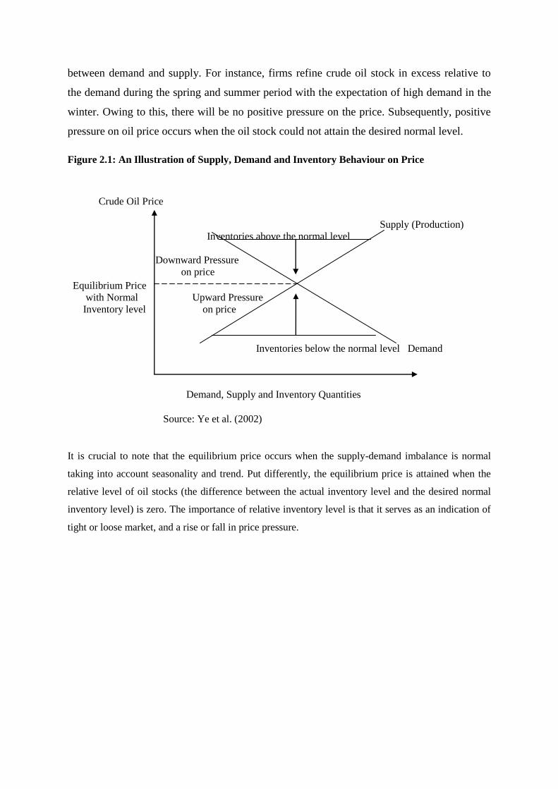
Figure 2.1: An Illustration of Supply, Demand and Inventory Behaviour on Price
Crude Oil Price
Supply (Production)
Inventories above the normal level
Downward Pressure
on price
Equilibrium Price
with Normal Upward Pressure
Inventory level on price
Inventories below the normal level Demand
Demand, Supply and Inventory Quantities
Source: Ye et al. (2002)
It is crucial to note that the equilibrium price occurs when the supply-demand imbalance is normal
taking into account seasonality and trend. Put differently, the equilibrium price is attained when the
relative level of oil stocks (the difference between the actual inventory level and the desired normal
inventory level) is zero. The importance of relative inventory level is that it serves as an indication of
tight or loose market, and a rise or fall in price pressure.

3. Methodology
3.1 Scope of Study
The study covers the US as one of net oil-importing countries in the world. Also, West Texas
Intermediate crude oil price is used since it is the international crude oil price in USA. This study
requires data on WTI crude oil price, crude oil stocks and other key economic variables such as
employment, OPEC production, OPEC refinery capacity and energy intensity from 1976 to 2009 for
its empirical analysis. Data on WTI crude oil price, crude oil stocks and energy intensity are obtained
from US Energy Information Administration (EIA). However, EIA only provides data from 1988 to
2009 for WTI crude oil prices; the remaining data prior to 1988 are obtained from BP statistical
reviews while the data on OPEC crude oil production and refinery capacity are collected from OPEC
Annual Statistical Bulletins. Data on employment level is obtained from US Bureau of Labour
Statistics.
Based on the previous studies and background knowledge, assumption was made that crude oil price
is influenced by inventory, OPEC production, OPEC refinery capacity, US employment and energy
intensity. The aim of this research is to estimate the long-run and short-run inventory, crude oil
production, refinery capacity, employment and energy intensity elasticities. The estimation of the
model is carried out using the co integration method.
3.2 Description of all variables in the study
3.2.1 WTI crude oil price
Figure 3.1 plots the WTI crude oil price in the period 1976-2009. There was increase in WTI price of
crude oil due to the 1990 Persian Gulf War, the PDVAS strike in late 2002, and Rita and Katrina
hurricanes in 2005. Prior to the Iraq war in 2003, oil supply shortage led to an increase in oil price.
The aforementioned events directly affect the supply side of crude oil market but the Asian crisis
which is a clear illustration of an exogenous demand shock resulted into a drastic fall in the crude oil
price in 1998 and 1999.

Figure 3.1: Historical Trend of Annual WTI Crude Oil Price
Data Source: US Energy Information Administration (EIA, 2009), Washington DC
3.2.2 US Crude Oil Inventory
Crude oil stock is the main factor that influences the short-run price of crude oil. However, many
other commodities are produced to meet their direct demand; oil producers use their crude oil stock
with the new production to balance demand level in the market. Obviously, inventories encourage
producers to respond to the unexpected market condition (supply- demand imbalance) by taking from
the existing crude oil stock. Figure 3.2 plots series of US crude oil inventory and WTI crude oil prices
(see Figure 1.1 for more detail of the analysis). However, a negative relationship is expected between
inventory and oil price based on economic theory described in Figure 2.1.
Figure 3.2: Historical Relationship between US Crude Oil Inventory and WTI Crude Oil Price
Data Source: US Energy Information Administration (EIA, 2009), Washington DC
0
20
40
60
80
100
120
1976 1979 1982 1985 1988 1991 1994 1997 2000 2003 2006 2009
US
Do
lla
rs p
er B
arr
el (
$/b
)
Years
WTI
0
20
40
60
80
100
120
0
200000
400000
600000
800000
1000000
1200000
1400000
19
76
19
78
19
80
19
82
19
84
19
86
19
88
19
90
19
92
19
94
19
96
19
98
20
00
20
02
20
04
20
06
20
08
US
Do
lla
rs p
er B
arr
el (
$/b
)
Th
ou
san
d B
arr
els
per
Day
INV WTI

3.2.3 OPEC Crude Oil Production
OPEC production, being the largest share of global production exhibits a significant influence on
crude oil price. Figure 3.3 plots this time series of OPEC production (denoted as OPP) in thousands
per day. Oil production witnessed a decline due to the Gulf War in 1990 and PDVAS strike in late
2002. However, the Asian crisis and the subsequent reduction in oil production in 1998 encouraged
the Oil prices to revert to their previous value. Obviously, oil producing nations responded slowly to
demand shocks due to the costs of adjusting oil production and the uncertain condition of the oil
market. A prior expectation is that OPEC production has a negative influence on WTI crude oil price.
Figure 3.3: Historical Relationship between OPEC Production (OPP) and WTI Crude Oil Price (WTI)
Data Source: US Energy Information Administration (EIA, 2009), Washington DC and OPEC Annual Statistical Bulletins (2009)
3.2.4 OPEC Refinery Capacity
Figure 3.4 plots the time series of refinery capacity denoted as OPR in thousands per day. The
increase in the refinery capacity encourages the production of crude oil which in turn leads to a rise in
the supply of crude oil. Consequently, this results into a fall in oil price. Economic theory suggests an
inverse relationship between the two variables.
0
20
40
60
80
100
120
0
5000
10000
15000
20000
25000
30000
35000
19
76
19
78
19
80
19
82
19
84
19
86
19
88
19
90
19
92
19
94
19
96
19
98
20
00
20
02
20
04
20
06
20
08
US
Do
lla
rs p
er B
arr
el (
$/b
)
Th
ou
san
d B
arr
els
per
Da
y
OPP
WTI

Figure 3.4: Historical Relationship between OPEC Refinery Capacity (OPR) and WTI Crude
Oil Price (WTI)
Data Source: US Energy Information Administration (EIA, 2009), Washington DC and OPEC Annual Statistical Bulletin (2009)
3.2.5 US Employment Level
This variable is used to capture the level of income in US. An increase in the level of employment
will make more people to earn income. Owing to this, more people will demand for crude oil products
which invariably increase the price for crude oil. Figure 3.5 plots the time series of employment
between 1976 and 2009 measured in thousands. In the light of this, a positive relationship is
theoretically expected to exist between employment and oil price.
Figure 3.5: Historical Relationship between US Employment Level (EMP) and WTI Crude Oil
Price (WTI)
Data Source: US Energy Information Administration (EIA, 2009), Washington DC and US Bureau of Labour Statistics (2009).
0
20
40
60
80
100
120
0
1000
2000
3000
4000
5000
6000
7000
8000
9000
10000
19
76
1978
19
80
19
82
19
84
1986
19
88
19
90
19
92
19
94
19
96
19
98
20
00
20
02
20
04
20
06
20
08
US
Do
lla
rs p
er B
arr
el (
$/b
)
Th
ou
san
d B
arr
els
per
Da
y
OPR
WTI
0
20
40
60
80
100
120
0
20000
40000
60000
80000
100000
120000
140000
160000
1976
1978
1980
1982
1984
1986
1988
1990
1992
1994
1996
1998
2000
2002
2004
2006
2008
US
Doll
ars
per
Barr
el (
$/b
)
US
Em
plo
ym
ent
Lev
el
(Th
ou
san
ds)
EMP
WTI

3.2.6 US Energy Intensity
The study adopts an index designed by US Energy Information Administration to measure the US
energy intensity. This index is calculated by dividing US annual energy consumption with US annual
real Gross Domestic Production. Figure 3.6 plots the index of US energy intensity during the period
1976-2009. A decline in the index implies improvement in energy efficiency vice versa. Therefore,
the index is used as the proxy for energy efficiency and a prior expectation is that the energy intensity
has positive influence on WTI crude oil price.
Figure 3.6: Historical Relationship between US Energy Intensity (EI) and WTI Crude Oil
Price (WTI)
Data Source: US Energy Information Administration (EIA, 2009), Washington DC
3.3 Model employed in the study
The study utilises the linear model to examine the relationship between WTI crude oil price and
Inventory using co integration techniques. The model includes the additional explanatory variables
(macroeconomic variables) such as OPEC crude oil Production, OPEC refinery capacity, US
employment and energy intensity. Inclusion of these variables in the models makes them structural
and inclusion of the lag of the variables makes them dynamic. Therefore, the model is regarded as the
structural dynamic model as indicated in the study title.
0
2
4
6
8
10
12
14
16
0
20
40
60
80
100
120
1976
1978
1980
1982
1984
1986
1988
1990
1992
1994
1996
1998
2000
2002
2004
2006
2008
En
ergy I
nte
nsi
ty I
nd
ex
US
Doll
ars
per
Barr
el (
$/b
)
WTI
EI

3.3.1 Description of Linear Model
This model is employed by modifying Salman‟s model (2006). The modification is made by
excluding the time trend and including macroeconomic variables because the time trend may not be
able to capture all other factors that might have influences on WTI crude oil price. Owing to this
reason, variables that can influence non- physical demand and supply of crude oil, which in turns
affects the WTI crude oil prices, are included in the model. The model examines the impact of
inventory, OPEC crude oil production, OPEC refinery capacity, US employment and energy intensity
on WTI crude oil price.
3.4 Methods of Estimation
The study aims to examine the long-term relationship between WTI crude oil Price and crude oil
inventory in US between 1976 and 2009. Employing co-integration and Vector Error Correction
Model (VECM) steps, the study will investigate the relationship between the two variables. The
possible short-run features of the relationship among WTI crude oil price and inventory are obtained
from the VECM application. Then, unit root, VAR, co-integration and Vector Error Correction Model
(VECM) steps will be exploited.
4. Presentation and Interpretation of Study Results
4.1 Data Sources
For the purpose of this study, all the variables analysed have been expressed in a logarithmic form.
This empirical study utilises the annual time-series data of WTI crude oil price, inventory, OPEC
crude oil production, OPEC refinery capacity, US employment and energy intensity for the 1976-2009
periods. The choice of the starting year is based on the availability of data on WTI crude oil price.
Also, the annual dataset employed in this study is due to non availability of quarterly data on some
variable such as employment and energy intensity. All the variables are expressed into natural
logarithm form in order to reduce the scale effect.

4.2 Unit Root Test and Order of integration
Table 4. 1: Summary of ADF tests of unit roots in the variables (with intercept and trend)
ADF (n): Augmented Dickey-Fuller with allowance for nth auto regressions. Note: Maximum Lag length of 4 is allowed in the unit root
tests based on Schwarz information criterion. Where LWTI is the natural logarithm of US West Texas Intermediate crude oil prices, LINV is
the natural logarithm of US crude oil inventory, LOPP is the natural logarithm of OPEC crude oil production, LOPR is the natural logarithm
of OPEC refinery capacity, LEMP is the natural logarithm of US employment level and LEI is the natural logarithm of US energy intensity.
Superscript A denote the ADF test for first difference with intercept only and superscript B denotes the ADF test for first difference without
intercept and no trend. For the graphical representation of the variables in level and first difference (see Appendix 1)
Table 4.1 presents the results of unit root tests based on augmented Dickey–Fuller (ADF) statistics on
the natural logarithms of the levels and the first differences of the variables. In ADF test, the null
hypothesis is that the series has a unit root against the alternative of stationarity. The results reveal
that all series are I (1) in nature. The results of the ADF test do not establish stationarity for the levels
of any of the series. So, there are sufficient reasons to accept the null hypothesis of a unit root for the
level series. For all the first differenced series, the ADF test suggests stationarity at the 5%
significance level.
Variables ADF(n) 1%
Critical
value
5%
Critical
value
10%
Critical
Value
LWTI -1.701 -4.263 -3.553 -3.210 Fail to reject the null at all significance levels
LINV -1.266 -4.263 -3.553 -3.210 Fail to reject the null at all significance levels
LOPP -3.392 -4.285 -3.563 -3.215 Fail to reject the null but not at 10% significance
level
LOPR -2.110 -4.263 -3.553 -3.210 Fail to reject the null at all significance levels
LEMP -1.007 -4.273 -3.558 -3.212 Fail to reject the null at all significance levels
LEI -1.828 -4.263 -3.553 -3.210 Fail to reject the null at all significance levels
ΔLWTIA -5.029 -3.654 -2.957 -2.617 Reject the null at all significance levels
ΔLINVA -5.537 -3.654 -2.957 -2.617 Reject the null at all significance levels
ΔLOPPB -2.229 -2.642 -1.952 -1.610 Reject the null at least at 5% significance level
ΔLOPRA -7.081 -3.654 -2.957 -2.617 Reject the null at all significance levels
ΔLEMPB -2.061 -2.639 -1.952 -1.611 Reject the null at least at 5% significance level
ΔLEIA -4.730 -3.654 -2.957 -2.617 Reject the null at all significance levels

4.3: Presentation of the Johansen Co-integration Results
Since the series examined have the same order of integration, this study is able to perform the
Johansen and Juselius co-integration procedure. Co-integration tests have been subsequently applied,
in order to find the long-run relationship between WTI crude oil price and inventory.
Table 4. 2: Selection of appropriate lag length
Lag FPE AIC SC HQ
0 9.53e-11 -6.07 -5.79 -5.98
1 5.76e-15 -15.81 -13.87* -15.18
2 8.63e-15 -15.69 -12.07 -14.51
3 1.72e-15* -18.18* -12.90 -16.46*
Note: * shows appropriate lag length for each criterion.
Table 4.2 shows the optimal lag length selected in accordance with Final Prediction Error (FPE),
Akaike Information Criterion (AIC), Schwarz Information Criterion (SC) and Hannan-Quinn
Information (HQ). As reported in Table 4-2, while Final Prediction Error (FPE), Akaike Information
Criterion (AIC) and Hannan-Quinn Information (HQ) suggest that the appropriate lag length for the
model is “3”, Schwarz Information Criterion (SC) on the other hand, suggests that the appropriate lag
length is 1.
Using a maximum likelihood procedure, the Johansen approach tests for the existence of co
integration among non-stationary variables, and estimates the number of co integrating vectors in a
multivariate context. If the co integration relationship is identified among the variables, then it is
possible to estimate the parameters of long-run and short-run relationship.
Based on the result of unit root test, it is plausible to consider that all variables as endogenous
variables in the unrestricted VAR model, which have long-run relationships and impacts. Initially, the
lengths of the lags of endogenous variables were set at 3 (see table 4.4). Then, through a testing
procedure and by using lag exclusion tests (Wald test) and lag length criteria (SC) suggested 1 in
the first place; the final lag length in the unrestricted VAR model was selected to be one.
The next step is the test for the existence and the number of co integrating vectors. Using both the
maximal eigenvalue test (Lmax) and the trace test ( Ltrace ), the table below illustrates the results of the
test using a 5% significance level.
A linear deterministic trend was imposed on the data, which allowed for an intercept and trend in the
VAR model, but not in the co integration equation.
4.3.1 Linear Inventory Model
In order to test the existence and the number of co integrating vector, both the maximal eigenvalue
test (Lmax) and the trace test (Ltrace) are used. The table below illustrates the results of the test using a
5% significance level.
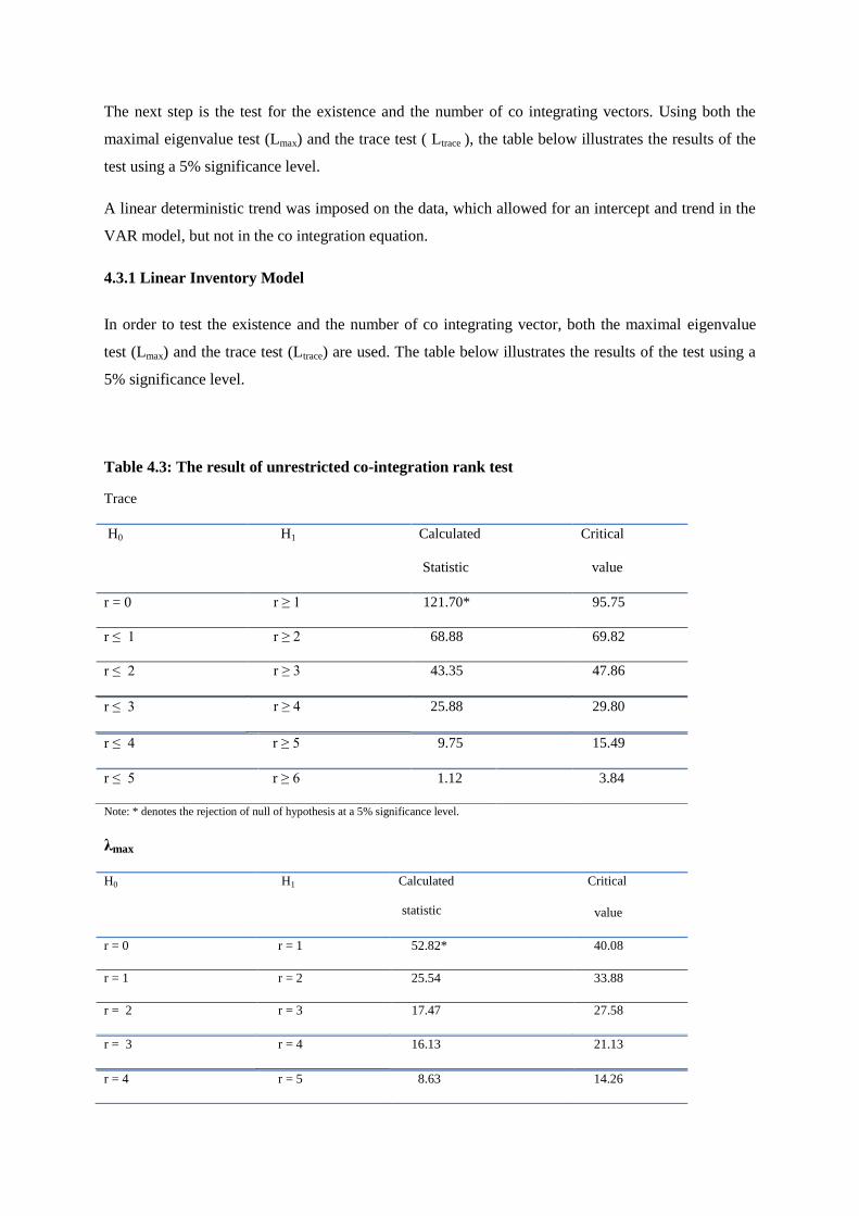
Table 4.3: The result of unrestricted co-integration rank test
Trace
r ≤ 3 r ≥ 4 25.88 29.80
Note: * denotes the rejection of null of hypothesis at a 5% significance level.
λmax
r = 3 r = 4 16.13 21.13
H0 H1 Calculated
Statistic
Critical
value
r = 0 r ≥ 1 121.70* 95.75
r ≤ 1 r ≥ 2 68.88 69.82
r ≤ 2 r ≥ 3 43.35 47.86
r ≤ 4 r ≥ 5 9.75 15.49
r ≤ 5 r ≥ 6 1.12 3.84
H0 H1 Calculated
statistic
Critical
value
r = 0 r = 1 52.82* 40.08
r = 1 r = 2 25.54 33.88
r = 2 r = 3 17.47 27.58
r = 4 r = 5 8.63 14.26

Note: * denotes the rejection of null of hypothesis at a 5% significance level.
Table 4.3 indicates the results of the johansen maximum likelihood co integration test using the
Eviews package. Starting with the null hypothesis of no co integration among the variables, H0: r0 = 0,
the trace test as shown in table 4.3, the null hypothesis of no co integration is rejected at the 5% level
of significance.
Hence, results of both tests imply that the hypothesis of no co integrating equation is rejected at the
5% significance level. Turning to the maximal eigenvalue statistic is 52.82; this is above the 5%
critical value of 40.08. Hence, the null hypothesis of r0 is rejected at the 5% level of significance.
However, under H0: r0 = 1, the trace and maximum eigenvalue statistics are 68.88 and 25.54, which
are below the 5% critical value of 69.82 and 33.88, respectively.
Hence, the null hypothesis is accepted at the 5% significance level. These results imply that the series
of the variables examined have one co-integrating equation; put differently, there is a long-run
relationship among WTI crude oil price, inventory, OPEC production, OPEC refinery capacity,
employment and energy intensity. Co-integration suggests the existence of Granger causality;
however, it does not indicate the direction of the causality relationship.
Table 4.4: Estimates of Unrestricted Co integrating Vectors (β) and Loading Factors (α)
Variables Β α
LWTI 1.00 0.10 (0.60)*
LINV 0.29 (5.83) -0.68 (1.67)*
LOPP 1.57 (5.69) -0.03 (-0.82)*
LOPR 9.22 (9.02) -0.10 (-3.96)
LEMP - 3.86 (-1.37) -0.02 (-2.82)
LEI 5.15 (3.77) -0.00(-0.46)*
C -71.09
Notes: t- statistics are given in parentheses and * denotes insignificant parameter.
r = 5 r = 6 1.12 3.84

Normalized for LWTIt , the unrestricted co integrating vector is given by
vt = LWTIt + 0.29LINVt + 1.57LOPPt + 9.22LOPRt − 3.86LEMPt + 5.15LEIt − 71.09 (4.1)
This can be written as
LWTIt = − 0.29LINVt − 1.57LOPPt − 9.22LOPRt + 3.86LEMPt − 5.15LEIt + 71.09 + vt (4.2)
As shown in Table 4.4, the t- statistics for the individual parameters (calculated by the method
suggested by Juselius and Hargreaves 1992) indicate that the parameters in the β vector except LEMP
are all individually significantly different from zero. Moreover, the co integration vectors have been
normalized by the WTI crude oil price coefficient. Consequently, the co integrating vectors associated
with LINV, LOPP, LOPR, LEMP and LEI can be considered as long-run inventory, production,
refinery capacity, employment and energy intensity elasticities of WTI crude oil price. In addition, all
the explanatory variables except energy intensity have correct signs as theoretically expected.
On the other hand, the loading factors associated with LWTI, LINV, LOPP and LEI were estimated to
be insignificant at 5% level of significance. In contrast, the loading factor for the LOPR and LEMP
are significantly different from zero with negative signs. This implies that the adjustment towards the
long-run equilibrium is governed by adjustment in the LOPR and LEMP.
The equation (4.2) indicates that in the long-run equilibrium, a 1% increase in inventory, crude oil
production, refinery capacity and energy intensity is accompanied by approximately 0.29%, 1.57%,
9.22% and 5.15% decrease in WTI crude oil prices respectively while a 1% rise in the US
employment level is accompanied by about 3.86% increase in WTI crude oil prices, ceteris paribus.
The t statistics for testing the significance of individual variables in the co-integrating vector indicates
that variables (LINV, LOPP, LOPR and LEI) are significant at 1% significance level while variable
LEMP is insignificant.
Table 4-5: VECM results (t-statistics in brackets)
ΔLWTI ΔLINV ΔLOPP ΔLOPR ΔLEMP ΔLEI
ECT 0.096
(0.605)
-0.679
(-1.666)
-0.040
(-0.823)
-0.100
(-3.955)
-0.018
(-2.818)
-0.004
(-0.465)
ΔLWTI(-1) -0.144
(-0.467)
1.413
(1.781)
0.015
(0.158)
0.130
(2.621)
0.006
(0.484)
-0.011
(-0.642)
ΔLINV(-1) -0.013
(-0.184)
0.046
(0.249)
-0.002
(-0.114)
0.014
(1.260)
-0.003
(-0.924)
-0.002
(-0.467)
ΔLOPP(-1) 0.277
(0.396)
0.656
(0.364)
0.218
(1.022)
0.155
(1.386)
-0.012
(-0.404)
0.053
(1.407)

ΔLOPR(-1) -0.581
(-0.470)
-0.131
(-0.041)
0.345
(0.920)
0.179
(0.905)
0.102
(1.997)
0.044
(0.668)
ΔLEMP(-1) 7.091
(1.189)
3.754
(0.245)
-0.432
(-0.238)
-1.826
(-1.913)
0.205
(0.834)
-0.171
(-0.535)
ΔLEI(-1) 3.650
(0.911)
-15.951
(-1.551)
2.032
(1.670)
-0.374
(-0.584)
-0.007
(-0.042)
0.084
(0.392)
C 0.034
(0.311)
-0.554
(-1.999)
0.040
(1.217)
0.027
(1.561)
0.007
(1.642)
-0.017
(-3.011)
Hence, starting with the error-correction term (ECT), the results as shown in Table 4.5 suggest that
the value of 0.096 for the coefficient of error correction term in the LWTI equation is not significant
and does not have a correct sign while for the other equations , the error correction terms coefficients
for LOPR and LEMP equations are negatively significant. This implies that the long-run
disequilibrium error of the LWTI equation is not influencing the LINV, LOPP and LEI equations but
influencing the LOPR and LEMP equations. In the short run LWTI equation, all the explanatory
variables are not significantly different from zero as indicated in the Table 4.5.
4.4 Interpretation of the Results
The above model is estimated using the co-integration techniques to examine the influence of crude
oil inventory on the WTI crude oil price. The linear inventory model is able to achieve the aim of this
study because crude oil inventory is inversely significant in determining the WTI crude oil price in the
model. In addition, this implies that the model is able to capture the influence of inventory on crude
oil prices in the short-run and long-run situations. Also, the result of the linear inventory model
conforms to the previous findings in the literature (Salman, 2006; Ze et al. 2002).
5. Conclusion
A policy implication of the results suggests that US should focus more attention on oil inventory as
this influences the WTI crude oil prices and since the OPEC production and refinery capacity are
beyond their control being the uncontrollable external influences. To address this influence of the oil
prices, US should rely more on its fiscal policy for oil inventory rather than monetary policy.
Based on the aforementioned findings, this study adds to the existing literature, as it has a particular
focus on the impact of crude oil inventory on the WTI crude oil price under examination. Also, it
examines a large economy such as US being the largest net oil-importing country in the world rather
than a regional economy which has been extensively studied in the past. Moreover, this study utilises
the recent annual data which consider the recent oil crisis period.
In conclusion, an interesting area for further research is to examine the relationship between
inventory and crude oil price using the structural dynamic model based on daily or weekly or monthly
or quarterly data rather than annual data employed in this study. Also, future research can look at the
relationship between the oil price and inventory in different regions in US in order to examine the
regional differences in terms of their relationship.
References
Antonio Merino and Rebecca Albacete (2010) “Econometric Modelling for Short –Term Oil Price Forecasting”
OPEC Energy Review: 25 -41.
Abosedra, S. (2005) “Futures versus Univariate Forecast of Crude Oil Prices”, OPEC Review, 29: 231–241.
Adnan, S., Bukhari, H.A.S, and Khan, S.U. (2008) “Estimating Output Gap for Pakistan Economy: Structural
and Statistical Approaches”, SBP Research Bulletin 4(1): 31-60.
Banerjee, A., Dolado, J., Galbraith, J.W and Hendry, D.F. (1993). Co-integration and Error Correction and the
Econometric Analysis of Non-stationary Data. Oxford: Oxford University Press.
Brennan, M. J. (1958) “The Supply of Storage”, American Economic Review 47.
BP Statistical Review of World Energy, June, 2010. Available at
http://www.bp.com/liveassets/bp_internet/globalbp/globalbp_uk_english/reports_and_publications/statistical_en
ergy_review_2008/STAGING/local_assets/2010_downloads/statistical_review_of_world_energy_full_report_2
010.pdf accessed on 15/07/2011
Bureau of Labour Statistics, Department of Labour, USA, 2011. Available at
http://www.bls.gov/news.release/empsit.a.htm accessed on 16/04/2011
Chernenko, S., Schwarz, K. and Wright, J.H. (2004) “The Information Content of Forward and Futures Prices:
Market Expectations and the Price of Risk”, FRB International Finance Discussion Paper 808.
Chin, M. D., LeBlanch, M. and Coibion, O. (2005) “The Predictive Content of Energy Futures: An Update on
Petroleum, Natural Gas, Heating Oil and Gasoline”, NBER Working Paper 11033.
Considine, T. J and Larson, D.F. (2001) “Risk Premiums on Inventory Assets: The Case of Crude Oil and
Natural Gas”, Journal of Future Markets 21(3).
Dale, Charles and Zyren John (1997) “Petroleum Future Markets: Volatile Prices, Controversial Functions and
Stagnant Volumes” Chapter 6, in Petroleum 1996: Issues and Trends, DOE/EIA-0615, Washington, DC.
Dees, S., Karadeloglou, P., Kaufmann, R.K and Sanchez, M. (2007) “Modelling the World Oil Market:
Assessment of a Quarterly Econometric Model” Energy Policy 35: 178–191.
Energy Information Administration (EIA), US Department of Energy, Washington DC, 2009.
Available at:
http://www.eia.gov/cfapps/ipdbproject/iedindex3.cfm accessed on 12/04/2011
Engle, R. F. and Granger, C.W.J (1987) “Co-integration and Error Correction: Representation, Estimation and
Testing” Econometrica 55(2): 251–276.
Granger, C. W. J. and Newbold, P (1974) “Spurious Regressions in Econometrics”, Journal of Econometrics 2:
111–120.
Gulen, S. G. (1988) “Efficiency in the Crude Oil Futures Markets”, Journal of Energy Finance and
Development 3: 13–21.
Harris, Richard and Sollis Robert (2003). Applied Time Series Modelling and Forecasting. England: John
Wiley& Sons
Hodrick, R. and Prescott, E. C. (1997) “Postwar US Business Cycles: An Empirical Investigation” Journey of
Money, Credit and Banking 29: 1-16.
Kaufmann, R. K. (1995) “A Model of the World Oil Market for Project LINK: Integrating Economics, Geology,
and Politics”, Economic Modelling 12: 165–178.

Kaufmann, R. K. (2004) “Does OPEC Matter? An Econometric Analysis of Oil Prices”, The Energy Journal 25:
67–91.
Lalonde, R., Zhu, Z and Demers, F. (2003) “Forecasting and Analyzing World Commodity Prices”, Bank of
Canada, Working Paper: 2003–24.
Merino, A. and Ortiz, A. (2003) “Explaining the So-called „Price Premium‟ in Oil Markets”, OPEC Review 29:
133–152.
Moosa, I. A., and Al-Loughani, N.E. (1994), “Unbiasedness and Time Varying Risk Premia in the Crude Oil
Futures Market”, Energy Economics 16: 99–105.
Morana, C. (2001) “A Semiparametric Approach to Short-term Oil Price Forecasting”, Energy Economics 23:
325–338.
Murat, A. and Tokat, E. (2009) “Forecasting Oil Price Movements with Crack Spread Futures” Energy
Economics 31: 85–90.
OPEC Annual Statistical Bulletin, 2004.Available at
http://www.opec.org/opec_web/static_files_project/media/downloads/publications/ASB2004.pdf accessed on
12/04/2011
OPEC Annual Statistical Bulletin, 2009. Available at
http://www.opec.org/opec_web/static_files_project/media/downloads/publications/ASB2009.pdf accessed on
12/04/2011
Pierse, R., MSc Econometrics Lecture Notes, University of Surrey, Department of Economics, Unpublished.
Pindyck, R. S. (1999) “The Long-run Evolution of Energy Prices”, The Energy Journal 20: 1–27.
Radchenko, S. (2005) “The Long-run Forecasting of Energy Prices Using the Model of Shifting Trend”
University of North Carolina at Charlotte, Working Paper.
Razak, W. (1997) “The Hodrick-Prescott Technique: A Smoother Versus a Filter: An Application to New
Zealand GDP”, Economics Letters 57 (2): 163-168.
Salman, S.G. (2006) “Assessment of the Relationship between Oil Prices and US Oil stock”, Energy Policy 34
(17): 3327-3333.
Samii, M. V (1992) “Oil Futures and Spot Markets”, OPEC Review 4: 409–417.
Sanders, D. R., Manfredo, M.R and Boris, K. (2009) “Evaluating Information in Multiple Horizon Forecasts:
The DOE‟s Energy Price Forecasts”, Energy Economics 31:189–196.
Schwartz, E. and Smith, J.E. (2000), “Short-term Variations and Long-term Dynamics in Commodity Prices”,
Management Science 46: 893–911.
Schwartz, E. and Smith, J. E. (1997) “The Stochastic Behaviour of Commodity Prices: Implications for
Valuation and Hedging”, Journal of Finance 51: 923–973.
Wikipedia, the Free Encyclopaedia. Available at:
http://en.wikipedia.org/wiki/Hodrick%E2%80%93Prescott_filter accessed on 25/08/2011
Williams, J.C and Wright, B.D. (1991) Storage and Commodity Markets. Cambridge: Cambridge University
Press.
Working, H. (1934) “Theory of Inverse Carrying Charge in Futures Markets”, Journal of Farming Economics
30.

Ye, M., Zyren, J. and Shore, J. (2002) “Forecasting Crude Oil Spot Price Using OECD Petroleum Inventory
Levels” International Advances in Economic Research 8 : 324–334.
Ye, M., Zyren, J. and Shore, J. (2005) “A Monthly Crude Oil Spot Price Forecasting Model Using Relative
Inventories”, International Journal of Forecasting 21: 491–501
Ye, M., Zyren, J. and Shore, J. (2006), “Forecasting Short-run Crude Oil Price Using High and Low Inventory
Variables”, Energy Policy 34: 2736–2743.
Zamani, M. (2004) “An Econometrics Forecasting Model of Short Term Oil Spot Price”, Paper presented at the
6th IAEE European Conference, Zurich, 2–3 September 2004.
Zeng, T. and Swanson, N.R. (1998) “Predictive Evaluation of Econometric Forecasting Models in Commodity
Future Markets” Studies in Nonlinear Dynamics and Econometrics 2: 159–177