Mohammad Dawude Temory

Impact of Agricultural Mechanization on Production and Income Generation in Afghanistan Case Study of Herat Province

Volume | 067 Bochum/Kabul | 2019 www.development-research.org | www.afghaneconomicsociety.org

1

Impact of Agricultural Mechanization on Production and Income Generation in Afghanistan

Case Study of Herat Province

Keywords

Agricultural Mechanization, Production, Productivity, Income Generation

Abstract

Agricultural mechanization is the utilization of different power sources and advanced farm tools

and equipment to decrease the drudgery of farmers and replace the use of draught animals. It helps

increase income, cropping intensity, production and efficiency, causing to the benefits different

crop inputs and decreasing the losses at different stages of crop production. The purpose of farm

mechanization is to increase overall production and income generation and to lower costs.

Agriculture is critical for Afghanistan’s food security and is a key driver of economic growth.

Most Afghan families live in rural areas and rely on agriculture and farming for their livelihoods

and to feed their families. Agriculture also creates employment and investment opportunities for

people living in urban areas.

This study found that agricultural mechanization has helped to increase the overall income and

production of farms in five districts of Herat Province. By applying the Cobb-Douglas production

function, we found that in our first model, which looks at crop production, farm size, quantity of

seed, quantity of fertilizer, irrigated area and quantity of agrochemicals all have a positive effect

on production: an increase or decrease in any of these inputs will increase or decrease production

respectively. In our second model, which looks at income, we found that price and production are

closely related to income. However, the other variables, including labor, education and experience,

are not associated with income at the farm level in the study area.

2

Description of Data

Both primary and secondary data were collected for this research. Primary data were gathered

through a standardized questionnaire survey. The sample was 400 farmers from five districts (Injil,

Guzara, Ghoryan, Pashtun Zarghun and Zinda Jan) of Herat Province. The questionnaire was

divided into three sections. The first section collected information on the demographic

characteristics of the farmers. This data was obtained to establish the structure of the farming

population in terms of their age, gender, household members, household size, and the educational

experience and other qualifications of the heads of households. The second section was the largest.

It collected data on the quantity of product, farm size, quantity of seed, quantity of fertilizer, labor

input, quantity of agrochemicals, farm assets, access to tractors, irrigated area and price of product.

Problems faced by the farmers were also included in this section. The last part of the questionnaire

asked about the farmers’ sources of income and expenditure. Before the individual interview, the

farmers had an interactive session where the questionnaire was explained to them.

The handwritten data recorded on the questionnaire sheets were checked for recording and transfer

errors, missing values, and outliers before being entered into a personal computer for analysis.

Secondary data were collected from the Ministry of Agriculture, Irrigation and Livestock of

Afghanistan. After the investigation, the data related to Herat was selected and used. The main

programs used for data analysis were the econometrics package Eviews 9, SPSS and Stata.

Microsoft Excel was used for some parts of the data analysis.

Research Question/Theoretical Contextualization

Afghanistan’s economy is dependent on the agricultural sector, which makes significant

contributions to food security, economic growth, poverty alleviation, employment enhancement,

and the fiscal health of the nation. For example, agriculture plays a significant role in the

livelihoods of the more than 80 percent of the country’s population and almost 90 percent of the

deprived who live in rural areas (World Bank, 2014). Therefore, agriculture is the most significant

economic activity and livelihood component in Afghanistan (NRVA, 2007).

Agriculture is also important for the growth and development of Afghanistan. This sector provides

employment for more than fifty percent of the population and contributes one quarter of gross

domestic product (GDP) (MAIL, 2017). Moreover, the existence of links between agriculture and

other sectors is vital for the growth and development of the country. For example, agriculture

provides raw materials and labor supply for industry, while the agricultural sector uses products

3

from the industrial sector, like machinery. Therefore, the lack of an effective agriculture sector can

affect both sectorial growth and the growth of the country.

Robert C. Hsu (1979) investigated the problems, policies and prospects of agricultural

mechanization in China. He found that as mechanization proceeds, the income inequality between

rural and urban areas decreases, while interactions between the two areas increase. He also added

that agricultural mechanization is accelerated by the technical skills of peasants and increases in

the supply of fertilizer and petroleum.

Verma (2008), in research on the “Impact of Agricultural Mechanization on Production,

Productivity, Cropping Intensity, Income Generation and Employment of Labour” in India, found

that mechanization leads to the development of new jobs such as managerial and supervisory jobs,

driving jobs, service jobs, and jobs in the maintenance and repair of machines. He also mentions

that farm mechanization has considerably assisted farmers, giving them overall economic

improvements.

Musa et. al (2012) used the investigative research approach to examine the effect of mechanization

on farm practices in north central Nigeria. They found that modern technology in agriculture has

strong potential for increasing farm productivity.

According to Ruttan & Hayami (1971) and Ruttan & Binswanger (1978), the rate and pattern of

mechanization is deeply influenced by the relative scarcities of capital and labor, and other

macroeconomic variables. The responsiveness of invention and innovation to economy-wide

factors has become recognized as induced.

Hans Binswanger (1986) clarified that mechanization is the main facilitator of the trend towards

bigger farms. Large farms adopt new forms of machinery considerably faster than small farms.

Muhammad Qasim (2012) applied the Cobb-Douglas production function and found that irrigated

areas, off-farm income, the number of livestock, hired labor and tractor ownership were positively

correlated with farm income.

Singh (2015) found that physical and institutional infrastructure, along with laws, regulations and

business-friendly policies, are the key factors in the success of agricultural mechanization in India.

Mankaran Dhiman and Jaskaran Dhiman (2015) believe that the mechanization of farm operations

has greatly assisted in reducing the labor requirements, drudgery and costs of cultivation, and helps

save farmers from vagaries of the weather. To make farmers globally competitive and prevent the

4

harm of natural resources, a major shift towards farm mechanization is required to realize the goal

of eco-friendly, sustainable agriculture with a low cost of production and high-quality produce.

Zaijion Yuan (2011) published a paper on agricultural input-output in northern China. He analyzed

agricultural input and output in the last ten years by applying the Cobb-Douglas production

function. He found that agricultural output, effective irrigation area, rural electricity consumption,

use of agricultural machinery and chemical fertilizer usage in Hebei Province are increasing, while

cultivated land area and rural manpower are decreasing. In this research we will also use the Cobb-

Douglas production function because of its many advantages, which are explained below.

The Cobb-Douglas production function (CDPF) is among the best production functions used in

applied production analysis (Enaami, et al., 2011). The Cobb-Douglas production function is

widely used in economic analysis to show the relationship of output to input (Qasim, 2012, p. 29).

The procedure was first suggested by Knut Wicksell (1851-1926). The formula was then tested

again by Charles Cobb and Paul Douglas in 1928. They investigated a simple way in which

production output is determined by the amount of labor and capital. It is one of the most important

methods used in many sectors, such as agriculture, education and health. This form of production

function has several advantages. For example, it is widely applied in economic and econometric

analysis and is flexible in the number of input variables used. Furthermore, economies of scale can

be computed as limited input coefficients that sum to one or without this limitation. In addition,

this method of production is easy to estimate and interpret. Using the CDPF unconstrained

increases its potential to handle different scales of production. Different econometrics estimation

problems, such as serial correlation, heteroscedasticity and multi-collinearity, can be handled

adequately and easily using this method. The only criticism of the model is lack of parsimony and

flexibility. This can be solved by making some assumptions in the model. The problem of

simultaneity can be accounted for by the use of a stochastic approach to the CDPF

(Bhamnumurthy, 2002, p. 75). The main characteristic of the CDPF is that the elasticity of

substitution is unified. The original form of the Cobb-Douglas production function is:

P = F(A K∝ Lβ) (1)

where

P = total production output (the monetary value of all goods produced)

K = capital input (the monetary worth of all equipment, buildings, machinery, etc.)

L = labor input (the total number of hours worked by people)

5

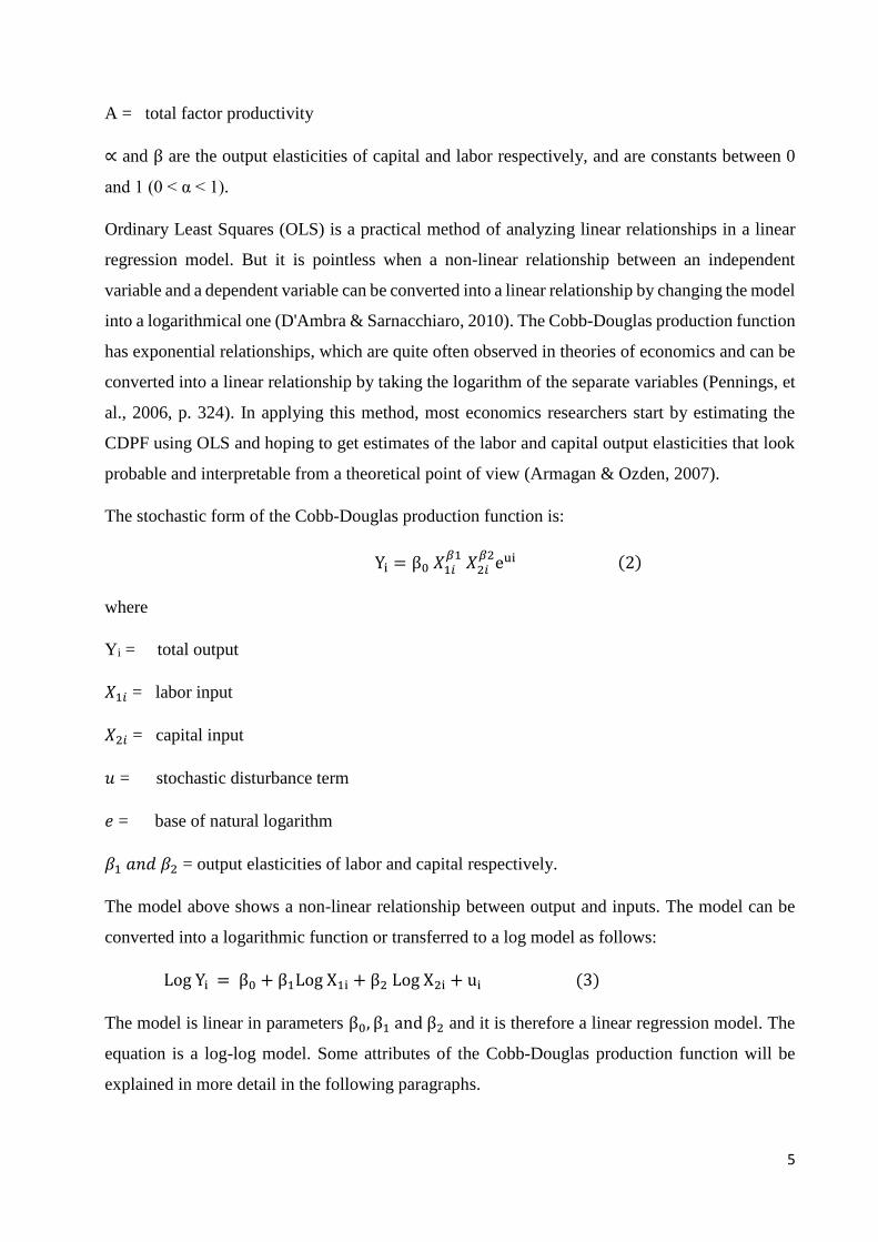
A = total factor productivity

∝ and β are the output elasticities of capital and labor respectively, and are constants between 0

and 1 (0 < α < 1).

Ordinary Least Squares (OLS) is a practical method of analyzing linear relationships in a linear

regression model. But it is pointless when a non-linear relationship between an independent

variable and a dependent variable can be converted into a linear relationship by changing the model

into a logarithmical one (D'Ambra & Sarnacchiaro, 2010). The Cobb-Douglas production function

has exponential relationships, which are quite often observed in theories of economics and can be

converted into a linear relationship by taking the logarithm of the separate variables (Pennings, et

al., 2006, p. 324). In applying this method, most economics researchers start by estimating the

CDPF using OLS and hoping to get estimates of the labor and capital output elasticities that look

probable and interpretable from a theoretical point of view (Armagan & Ozden, 2007).

The stochastic form of the Cobb-Douglas production function is:

Yi = β0 𝑋1𝑖𝛽1

𝑋2𝑖𝛽2

eui (2)

where

Yi = total output

𝑋1𝑖 = labor input

𝑋2𝑖 = capital input

𝑢 = stochastic disturbance term

𝑒 = base of natural logarithm

𝛽1 𝑎𝑛𝑑 𝛽2 = output elasticities of labor and capital respectively.

The model above shows a non-linear relationship between output and inputs. The model can be

converted into a logarithmic function or transferred to a log model as follows:

Log Yi = β0 + β1Log X1i + β2 Log X2i + ui (3)

The model is linear in parameters β0, β1 and β2 and it is therefore a linear regression model. The

equation is a log-log model. Some attributes of the Cobb-Douglas production function will be

explained in more detail in the following paragraphs.

6

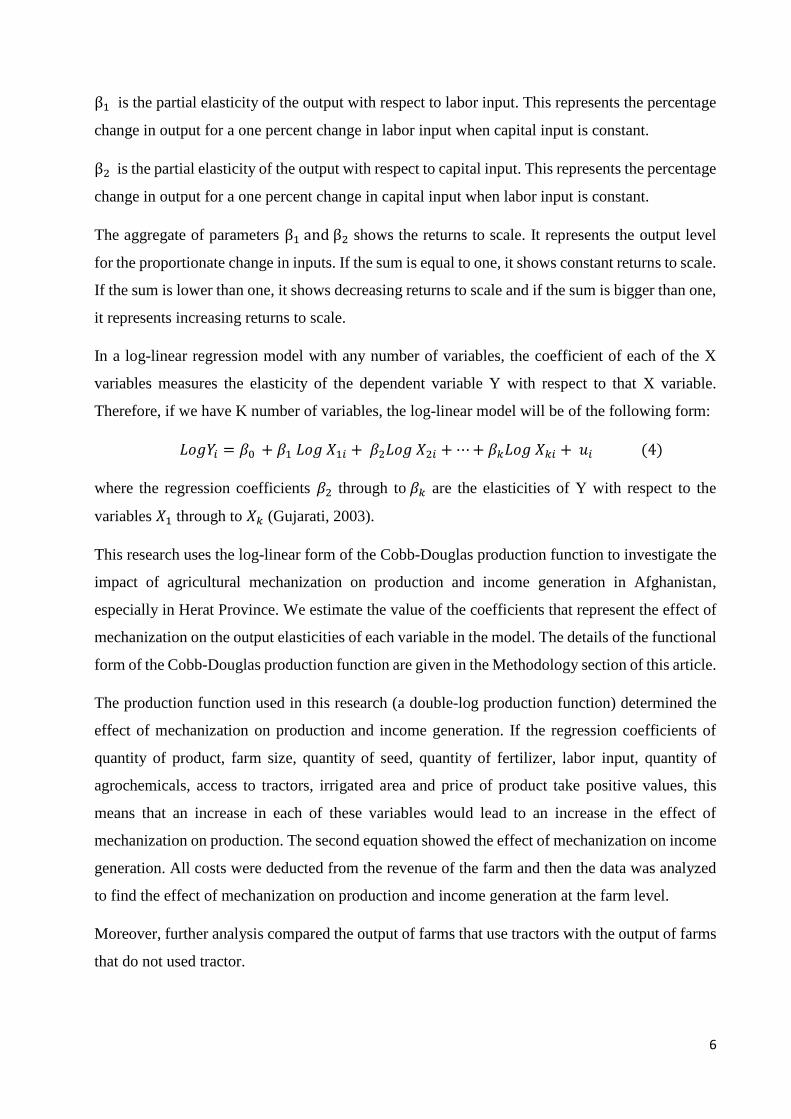
β1 is the partial elasticity of the output with respect to labor input. This represents the percentage

change in output for a one percent change in labor input when capital input is constant.

β2 is the partial elasticity of the output with respect to capital input. This represents the percentage

change in output for a one percent change in capital input when labor input is constant.

The aggregate of parameters β1 and β2 shows the returns to scale. It represents the output level

for the proportionate change in inputs. If the sum is equal to one, it shows constant returns to scale.

If the sum is lower than one, it shows decreasing returns to scale and if the sum is bigger than one,

it represents increasing returns to scale.

In a log-linear regression model with any number of variables, the coefficient of each of the X

variables measures the elasticity of the dependent variable Y with respect to that X variable.

Therefore, if we have K number of variables, the log-linear model will be of the following form:

𝐿𝑜𝑔𝑌𝑖 = 𝛽0 + 𝛽1 𝐿𝑜𝑔 𝑋1𝑖 + 𝛽2𝐿𝑜𝑔 𝑋2𝑖 + ⋯ + 𝛽𝑘𝐿𝑜𝑔 𝑋𝑘𝑖 + 𝑢𝑖 (4)

where the regression coefficients 𝛽2 through to 𝛽𝑘 are the elasticities of Y with respect to the

variables 𝑋1 through to 𝑋𝑘 (Gujarati, 2003).

This research uses the log-linear form of the Cobb-Douglas production function to investigate the

impact of agricultural mechanization on production and income generation in Afghanistan,

especially in Herat Province. We estimate the value of the coefficients that represent the effect of

mechanization on the output elasticities of each variable in the model. The details of the functional

form of the Cobb-Douglas production function are given in the Methodology section of this article.

The production function used in this research (a double-log production function) determined the

effect of mechanization on production and income generation. If the regression coefficients of

quantity of product, farm size, quantity of seed, quantity of fertilizer, labor input, quantity of

agrochemicals, access to tractors, irrigated area and price of product take positive values, this

means that an increase in each of these variables would lead to an increase in the effect of

mechanization on production. The second equation showed the effect of mechanization on income

generation. All costs were deducted from the revenue of the farm and then the data was analyzed

to find the effect of mechanization on production and income generation at the farm level.

Moreover, further analysis compared the output of farms that use tractors with the output of farms

that do not used tractor.

7

Research Objectives:

1- To analyze the impact of agricultural mechanization on production and income generation

in Afghanistan.

2- To identify the factors that drive the adoption of mechanization in Afghanistan.

3- To assess the current level of mechanization in the selected research areas.

4- To provide policy recommendations to the relevant government ministries and

international donors.

5- To compare the level of mechanization in five districts.

Research Questions:

1- Does agricultural mechanization affect production and income generation at the farm level

in Herat?

2- Does the effect of mechanization on output differ at the farm level?

3- What are the factors that drive the adoption of mechanization in Herat?

4- Does the level of mechanization differ in different parts of the research area?

Field Research Design/ Methods of Gathering Data

The main purpose of this study was to determine the impact of agricultural mechanization on

production and income generation in Afghanistan. In order to achieve this objective, primary data

were collected from five districts of Herat province. These five districts were selected for two

reasons:

1) They are the most populated districts, and thousands of families living in these districts work in

the agricultural sector.

2) These districts are more accessible for the field research compared to other areas of the province

and have better security than the other districts. Additionally, it was possible to obtain assistance

in making contact with farmers and attracting support for the field research process from the

department of agriculture. Primary data collection involved a sample survey, which was conducted

in the study locations during the period March - June 2019. The survey involved interviewing 400

farmers in the study locations (Injil, Guzara, Ghoryan, Pashtun Zarghun and Zinda Jan). Secondary

data sources, including reports, were used by the researcher. Sample farmers were selected using

the stratified random sampling method.

8

Table 1: Distribution of sample size in the selected districts

District Population Percentage Sample Size

Injil 233,900 38 152

Guzara 140,300 23 92

Ghoryan 84,300 14 56

Zinda Jan 54,600 9 36

Pashtun Zarghun 95,900 16 64

Total 609,000 100 400

Source: CSO (2011-2012)

Two models, both in the form of the Cobb-Douglas production function, were used to analyze the

data. The first model investigated the level of production and the second model investigated the

effect of mechanization on income generation at the farm level. The Cobb-Douglas production

function was used because it has many advantages and is used by many researchers in different

fields, especially in applied economics and econometrics. Furthermore, it is a very flexible

function and allows the researcher to use several input variables to investigate the effect of each

variable on the production process. The most important property of the function is its elasticity of

substitution (Mohammad Abdallah Khreisat 2011 p. 36).

In this research, econometrics instrumentations were used to establish the effect of mechanization

on production and income generation in Herat Province. A log function model of the Cobb-

Douglas production function was used with the Ordinary Least Squares (OLS) method to verify

the relationship between input and output (independent variable and dependent variable)

(Muhammad Qasim 2012 p. 99).

We used the Cobb-Douglas production function to investigate the level of production:

𝑌 = 𝑓( 𝑋1, 𝑋2, 𝑋3,𝑋4, 𝑋5,𝑋6,𝑋7, 𝑋8, 𝑈𝑖) (5)

where

𝑌 is the quantity of crop produced (kg)

𝑋1 is the farm size (hectares)

𝑋2 is the quantity of seed (kg)

9

𝑋3 is the quantity of fertilizer (kg)

𝑋4 is the labor input (man-days)

𝑋5 is the quantity of agrochemicals (liters)

𝑋6 is the access to tractors

𝑋7 is the irrigated area (hectares)

𝑋8 is the farmers’ education (years)

𝑈𝑖 are the error terms.

This function takes the following form:

𝐿𝑜𝑔𝑌 = 𝛽0 + 𝛽1 𝑙𝑜𝑔𝑋1 + 𝛽2𝑙𝑜𝑔𝑋2 + 𝛽3𝑙𝑜𝑔𝑋3 + 𝛽4𝑙𝑜𝑔𝑋4 + 𝛽5𝑙𝑜𝑔𝑋5 + 𝛽6𝑙𝑜𝑔𝑋6 + 𝛽7𝑙𝑜𝑔𝑋7

+ 𝛽8𝑙𝑜𝑔𝑋8 + 𝑈𝑖 (𝑑𝑜𝑢𝑏𝑙𝑒𝑙𝑜𝑔) (6)

In the second model we investigated the effect of mechanization on income generation at the farm

level:

𝑌 = 𝑓( 𝑋1, 𝑋2, 𝑋3,𝑋4, 𝑋5, 𝑈𝑖) (7)

where

𝑌 is the amount of income (US$)

𝑋1 is the price of product (US$)

𝑋2 is the quantity of crop produced (kg)

𝑋3 is the farmers’ education (years)

𝑋4 is the labor input (man-days)

𝑋5 is the farmers’ experience (years)

𝑈𝑖 are the error terms.

This function takes the following form:

𝐿𝑜𝑔𝑌 = 𝛽0 + 𝛽1 𝑙𝑜𝑔𝑋1 + 𝛽2𝑙𝑜𝑔𝑋2 + 𝛽3𝑙𝑜𝑔𝑋3 + 𝛽4𝑙𝑜𝑔𝑋4 + 𝛽5𝑙𝑜𝑔𝑋5

+ 𝑈𝑖 (𝑑𝑜𝑢𝑏𝑙𝑒𝑙𝑜𝑔) (8)

10

Results

As mentioned in the field research design section of this article, the primary data was collected

from five districts in Herat Province (Injil, Guzara, Ghoryan, Pashtun Zarghun and Zinda Jan)

through a standard questionnaire that contained 25 questions in three sections. The data were

analyzed with the following two models.

Empirical Analysis:

The following equations were used to determine the effects of mechanization on production and

income generation in the research area.

𝐿𝑜𝑔𝑌 = 𝛽0 + 𝛽1 𝑙𝑜𝑔𝑋1 + 𝛽2𝑙𝑜𝑔𝑋2 + 𝛽3𝑙𝑜𝑔𝑋3 + 𝛽4𝑙𝑜𝑔𝑋4 + 𝛽5𝑙𝑜𝑔𝑋5 + 𝛽6𝑙𝑜𝑔𝑋6 + 𝛽7𝑙𝑜𝑔𝑋7

+ 𝛽8𝑙𝑜𝑔𝑋8 + 𝑈𝑖 (9)

𝐿𝑜𝑔𝑌 = 𝛽0 + 𝛽1 𝑙𝑜𝑔𝑋1 + 𝛽2𝑙𝑜𝑔𝑋2 + 𝛽3𝑙𝑜𝑔𝑋3 + 𝛽4𝑙𝑜𝑔𝑋4 + 𝛽5𝑙𝑜𝑔𝑋5 + 𝑈𝑖 (10)

The above equations explain the relationship between all the independent variables and the

dependent variable. In the first equation, the data on the effect of mechanization on production

were analyzed with all control variables. In the second equation, the control variables, including

price of product, level of production, farmers’ education, labor input and farmers’ experience were

analyzed. The descriptive statistics were also analyzed and are depicted in Table 2.

Table 2: Descriptive Statistics

N Minimum

Maximu

m Mean

Std.

Deviation Variance

Farm size 400 1.00 10.00 2.6275 1.00312 1.006

Labor 400 1.00 35.00 3.6050 2.88788 8.340

Tractors 400 0.00 8.00 4.1025 1.71883 2.954

Education 400 0.00 8.00 2.2050 1.13631 1.291

Experience 400 1.00 6.00 2.9775 1.16421 1.355

Valid N (listwise) 400

Table 2 shows the descriptive statistics for the study area. The average farm size was 2.6 hectares,

the average amount of labor working on the land was 3.6 persons per hectare, the average number

of tractors each farmer had access to was 4.1, the education of farmers in the study area was on

average 2.2 years and the average experience of farmers in all districts was 2.9 years.

11

Table 3: Effects of Mechanization on Production and Income Generation

Note: values in parentheses are percentages

Table 3 highlights that agricultural production is significantly higher with than without

mechanization. It shows that production has increased by 113.8 percent or 36,241,941 kg overall,

and income has increased by 93.8 percent (34,283,707 AFA, equivalent to 42,329 US$).

Comparing the districts, we found that agricultural mechanization has made a substantial

contribution to increasing agricultural production. Injil district has benefited the most from

mechanization. In this district, production increased by 125 percent and income by 115 percent.

Zinda Jan district benefited from mechanization less than the other districts in the study area. Here

production increased 76 percent while income increased 59 percent.

Results of the First Model

The first model investigates the effect of mechanization on production at the farm level. This

model shows that farm size, seed, fertilizer, irrigation and agrochemicals are highly significant and

have a positive impact on production. It indicates that a one percent increase in each of the

variables will cause an increase of more than one percent in the total production at the farm level.

The labor variable is also significant but has a minus sign. The results are illustrated in Table 4.

District

Production

with

Mechanization

Production

without

Mechanization

Difference Income with

Mechanization

Income

without

Mechanization

Difference

Injil 27,647,275

(41.11)

12,278,470

(39.60)

15,368,805

(125)

25,221,320

(37.58)

11,733,143

(35.74)

13,488,177

(115)

Guzara 14,508,312

(21.57)

7,426,015

(23.95)

7,082,297

(95)

12,916,250

(19.24)

6,352,770

(19.35)

6,563,480

(103)

Ghoryan 11,121,751

(16.54)

4,099,600

(13.22)

7,022,151

(171)

11,487,991

(17.12)

7,012,700

(21.36)

4,475,291

(64)

Zinda Jan 3,932,130

(5.84)

2,230,370

(7.19)

1,701,760

(76)

3,657,674

(5.54)

2,300,160

(6.80)

1,357,514

(59.01)

Pashtun

Zarghun

10,031,898

(14.92)

4,964,970

(16.01)

5,066,928

(102)

12,821,645

(19.10)

6,392,400

(19.47)

6,429,245

(101)

Average

Changes in

Income &

Production

113.8 93.8

12

Table 4: Effect of Mechanization on Production

Model

Unstandardized Coefficients

t Sig. B Std. Error

(Constant) 3.749 0.113 33.189 0.000

Log farm size 0.401 0.084 4.788 0.000

Log seed 0.179 0.017 10.666 0.000

Log fertilizer 0.053 0.010 5.365 0.000

Log labor -0.127 0.047 -2.666 0.008

Log irrigation 0.024 0.011 2.127 0.034

Log agrochemicals 0.058 0.011 5.275 0.000

Log tractors 0.037 0.074 0.505 0.614

Education 0.011 0.012 0.916 0.360

Experience 0.004 0.013 0.338 0.736

Dependent variable: log production

Farm size, seed, fertilizer, irrigation and agrochemicals all have a positive effect on production.

An increase or decrease in these inputs will increase or decrease the production at the farm level

respectively because the signs of these variables’ coefficients are positive. However, labor has a

negative relationship with production, which means an increase in labor may directly decrease

production at the farm level.

Table 5: Analysis of Variance (ANOVA)

Model Sum of Squares df Mean Square F Sig.

Regression 15.629 9 1.737 23.495 0.000b

Residual 28.825 390 0.074

Total 44.453 399

a. Dependent variable: log production

b. Predictors: (constant), experience, log agrochemicals, log fertilizer, log seed, log labor,

log irrigation, log farm size, education, log tractors

Table 5 shows that the regression model predicts the dependent variable (quantity of crop

produced) significantly well. The F value is 23.49 and the P-Value is 0.000, indicating that overall

the regression model is statistically significant and shows a good fit for the data set.

13

Table 6: Model Summary

Model R R Square Adjusted R Square

Std. Error of the

Estimate

1 0.593a 0.352 0.337 0.27186

a. Predictors: (constant), experience, log agrochemicals, log fertilizer, log seed, log labor, log

irrigation, log farm size, education, log tractors

Table 6 shows how much changes in the quantity of crop produced are explained by changes in

farm size, seed, fertilizer, irrigation, agrochemicals, labor, education and experience. The value of

R square shows that almost 35.2 percent of the variance or changes in the quantity of crop produced

are influenced by all the independent variables that are already used in the forecasting of the model.

However, 64.8 percent of the changes in production are caused by other factors that are not directly

connected with the quantity of crop produced.

Results of the Second Model

The second model investigates the effect of mechanization on income generation in the study area.

The model examines the impact of changes in price, production, labor, farmers’ education and

farmers’ experience on income generation at the farm level. After running the regression on the

data set, the following results were obtained.

Table 7: Effect of Mechanization on Income Generation

Model

Unstandardized Coefficients

t Sig. B Std. Error

(Constant) 0.895 0.097 9.230 0.000

Log price 0.121 0.007 17.215 0.000

Log production 0.765 0.020 38.206 0.000

Log labor -0.017 0.033 -0.513 0.608

Experience 0.003 0.008 0.325 0.745

Education 0.003 0.009 0.367 0.714

a. Dependent variable: log income

Table 7 provides some information regarding the changes in income that would occur due to

changes in each of the independent variables in the model. The results of the model show that price

and production are highly related to income because the coefficient of these variables is highly

significant. The other variables, including labor, education and experience, are not related to

income at the farm level in the study area.

14

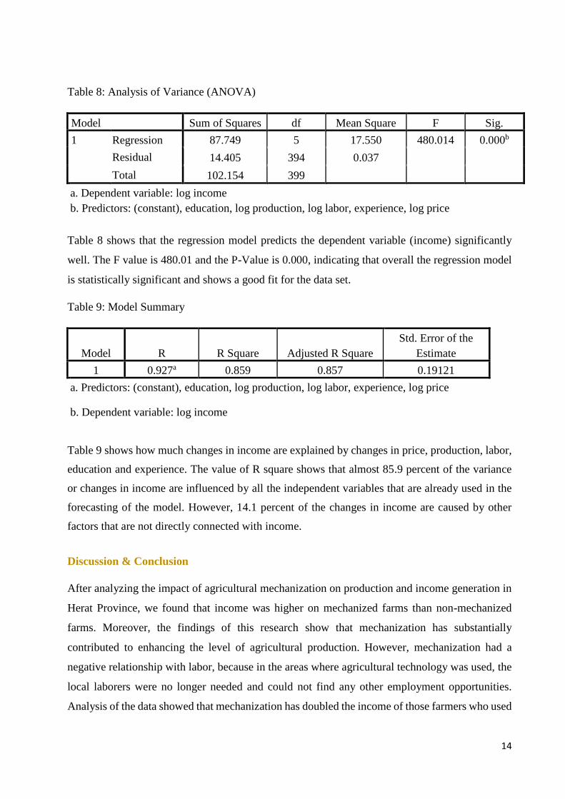
Table 8: Analysis of Variance (ANOVA)

Model Sum of Squares df Mean Square F Sig.

1 Regression 87.749 5 17.550 480.014 0.000b

Residual 14.405 394 0.037

Total 102.154 399

a. Dependent variable: log income

b. Predictors: (constant), education, log production, log labor, experience, log price

Table 8 shows that the regression model predicts the dependent variable (income) significantly

well. The F value is 480.01 and the P-Value is 0.000, indicating that overall the regression model

is statistically significant and shows a good fit for the data set.

Table 9: Model Summary

Model R R Square Adjusted R Square

Std. Error of the

Estimate

1 0.927a 0.859 0.857 0.19121

a. Predictors: (constant), education, log production, log labor, experience, log price

b. Dependent variable: log income

Table 9 shows how much changes in income are explained by changes in price, production, labor,

education and experience. The value of R square shows that almost 85.9 percent of the variance

or changes in income are influenced by all the independent variables that are already used in the

forecasting of the model. However, 14.1 percent of the changes in income are caused by other

factors that are not directly connected with income.

Discussion & Conclusion

After analyzing the impact of agricultural mechanization on production and income generation in

Herat Province, we found that income was higher on mechanized farms than non-mechanized

farms. Moreover, the findings of this research show that mechanization has substantially

contributed to enhancing the level of agricultural production. However, mechanization had a

negative relationship with labor, because in the areas where agricultural technology was used, the

local laborers were no longer needed and could not find any other employment opportunities.

Analysis of the data showed that mechanization has doubled the income of those farmers who used

15

tractors and other farm technology compared to those who did not. Comparing the different

districts in the study area, Zinda Jan district benefited the least from agricultural mechanization,

while Injil District benefited the most. The findings of the first model in this study, which analyzed

production, show that farm size, seed, fertilizer, irrigation and agrochemicals all have a positive

relationship with production, which means that an increase or decrease of these inputs will cause

an increase or decrease respectively in production. In the second model, which analyzed income,

it was found that price and production are highly related to income. However, the other variables,

including labor, education and experience, are not associated with income at the farm level in the

study area.

16

References

1- Armagan, G. & Ozden, A., (2007): Determinations of total factor productivity with Cobb-

Douglas production function in agriculture: The case of Aydin-Turkey. Journal of Applied

Sciences, Volume 7, pp. 499-502.

2- Bhamnumurthy, K. V., (2002): Arguing A Case for The Cobb-Douglas Production

Function. Review of Commerce Studies 2002, Delhi, India: s.n.

3- Binswanger, Hans P. 1978. The Economics of Tractors in South Asia: An Analytical

Review. New York: Agricultural Development Council; and Hyderabad, India: International

Crops Research Institute for the Semi-Arid Tropics.

4- Binswanger, Hans P. & Ruttan, Vernon W. 1978. Induced Innovation: Technology,

Institutions, and Development. Baltimore, Md.: Johns Hopkins University Press.

5- Chancellor, W. 1998. “Agricultural Mechanization: A History of Research at IRRI and

Changes in Asia.” In Increasing the Impact of Engineering in Agricultural and Rural

Development, edited by M. A. Bell, D. Dawe, and M. B. Douthwaite. IRRI Discussion Paper

Series No. 30. Los Baños, Philippines: International Rice Research Institute.

6- D'Ambra, A. & Sarnacchiaro, P., (2010): Some data reduction methods to analyze the

dependence with highly collinear variables: A simulation study. Asian Journal of Mathematics &

Statistics, Volume 3(2), pp. 69-81.

7- Enaami, M., Ghani, S. A. & Mohamed, Z., (2011): Multicollinearity Problem in Cobb-

Douglas Production Function. Journal of Applied Sciences, Volume 11(16), pp. 3015-3021.

8- Gujarati, D. N., (2003): Basic Econometrics. Published Book Fourth Edition. ISBN 0-07-

112342-3. In: s.l.: s.n., pp. 223-224.

9- Liu, Xianzhou. 1962. "The Invention of Agricultural Machinery in Ancient China." Acta

Agromechanica Sinica 5, no. 1:1-36; no. 2:1-48.

10- Pennings, P., Hans, K. & Kleinnijenhuis, J., (2006): Doing Research in Political Science.

In: s.l.: Sage USA, p. 324.

11- Qasim, M., (2012): Determinants of Farm Income and Agricultural Risk Management

Strattegies, PhD Thesis, Kassel: s.n.

12- World Bank, 2014. Agricultural Sector Review, Revitalizing Agriculture for Economic

Growth, Job Creation and Food Security.

13- http://cso.gov.af/Content/files/ALCS/NRVA%202007-08%20Main%20report.pdf

14- http://mail.gov.af/en/tender