
IMAGE STITCHING APPROACH USING MINIMUM AVERAGE … · tunjang manusia dan tangan yang bertindih dan...
87
IMAGE STITCHING APPROACH USING MINIMUM AVERAGE CORRELATION ENERGY SITI SALBIAH BINTI SAMSUDIN FACULTY OF ENGINEERING UNIVERSITY OF MALAYA KUALA LUMPUR 2012
Transcript of IMAGE STITCHING APPROACH USING MINIMUM AVERAGE … · tunjang manusia dan tangan yang bertindih dan...

IMAGE STITCHING APPROACH USING
MINIMUM AVERAGE CORRELATION ENERGY
SITI SALBIAH BINTI SAMSUDIN
FACULTY OF ENGINEERING
UNIVERSITY OF MALAYA
KUALA LUMPUR
2012

IMAGE STITCHING APPROACH USING
MINIMUM AVERAGE CORRELATION ENERGY
SITI SALBIAH BINTI SAMSUDIN
THESIS SUBMITTED IN FULFILMENT OF THE
REQUIREMENTS FOR THE DEGREE OF
MASTER OF ENGINEERING SCIENCE
FACULTY OF ENGINEERING
UNIVERSITY OF MALAYA
KUALA LUMPUR
2012
ii
Abstract
Panorama Image Stitching has been the subject of interest over the decades. A
panorama image is the output of blending a set of overlapping images taken at different
viewpoints. This process of producing a panorama image is called image stitching,
which consists of image registration and image blending. In this thesis, an image
stitching method that utilizes Minimum Average Correlation Energy (MACE) filters is
used to merge a number of overlapping images. Two sets of analysis were conducted to
measure the effectiveness of the proposed method using natural images and radiology
medical images. The performance of the proposed method is then compared to those of
two correlation based methods namely the Phase Only Correlation (POC) and
Normalized Cross Correlation (NCC) methods on the same databases. In the first set of
analysis, pair of overlapping and non-overlapping x-ray images of human spine and
hand was presented to the system to be merged if they were related or rejected if
otherwise. In the second set of analysis involving images of natural scenery, a number
of overlapping images were presented to the system to test its ability to recognize the
correct matching points to merge them. Then pairs of non-overlapping images were
introduced to the system to check whether the system able to identify that if they were
not related and should not be merged. In both analyses, it was found that the proposed
method outperformed the POC and NCC methods in identifying both the overlapping
and non-overlapping images. The efficacy of the proposed method is further vindicated
by its average execution time which is about two and five times shorter than those of
the POC and NCC method respectively.

iii
Abstrak
Imej penampalan panorama telah menjadi subjek yang penting selama beberapa dekad.
Imej panorama merupakan hasil adunan dari beberapa set imej yang bertindih diambil
pada pandangan berlainan. Proses menghasilkan imej panorama dipanggil imej
tampalan yang mengadungi pendaftaran imej and pengadunan imej. Di dalam tesis ini,
kaedah penampalan imej yang menggunakan penapis tenaga korelasi purata terendah
(MACE) di gunakan untuk menggabungkan beberapa imej yang bertindih. Dua set
eksperimen telah dijalankan untuk mengukur keberkesanan kaedah yang di
dicadangkan menggunakan imej semulajadi dan imej radiologi perubatan. Prestasi
kaedah baru ini kemudian dibandingkan dengan dua lagi kaedah berasaskan korelasi
yang dinamakan hanya fasa korelasi (POC) dan ternormal silang korelasi (NCC) pada
data-data yang sama. Dalam set eksperimen pertama, pasangan imej x-ray tulang
tunjang manusia dan tangan yang bertindih dan tidak bertindih dipersembahkan kepada
sistem untuk digabungkan jika mereka berkaitan atau ditolak jika sebaliknya. Pada set
kedua eksperimen yang melibatkan imej pemandangan semulajadi, beberapa imej yang
bertindih telah dipersembahkan pada sistem untuk menguji kebolehan nya mengenal
titik sepadan yang betul untuk digabungkan. Kemudian pasangan untuk imej tidak
bertindih diperkenalkan pada sistem untuk menyemak samaada sistem boleh
mengenalpasti mereka tidak berkaitan dan tidak patut digabungkan. Dalam kedua-dua
eksperimen, didapati kaedah yang baru mengatasi kaedah POC dan NCC dalam
mengenalpasti kedua-dua imej bertindih dan tidak bertindih. Keberkesanan keadah
yang dicadangkan disahkan lagi dengan purata masa pelaksanaan dimana kira-kira dua
dan lima kali lebih pendek berbanding dengan kaedah POC dan NCC masing-masing.

iv
Acknowledgement
This research project would not have been possible without the support of many
people. I am heartily thankful to my supervisor Dr. Hamzah arof who was very helpful
and offered invaluable assistance, support and guidance. Not forgetting my second
supervisor, Associate Prof. Dr. Fatimah Ibrahim for her guidance and assistant through
monthly colloquium. Deepest gratitude is also to, Dr. Somaya whose knowledge and
assistance have made this study successful.
I would also like to convey thanks to the Ministry and Faculty for providing the
financial means and laboratory facilities under grant number PS144-2010A. Thanks
also to Puan Norrima who had support me for RA scholarship for 1 year under UMRG
grant.
I would like to express my love and gratitude to my beloved families; for their
understanding and endless love, through the duration of my studies. Not forgetting to
my best friends Roziana, Fadzilah and zaki who always been there.

v
Table of Contents
CHAPTER 1 .................................................................................................................................. 1
Introduction ............................................................................................................................... 1
1.1 Chapter Overview ....................................................................................................... 1
1.2 Background study ....................................................................................................... 1
1.3 Thesis Objectives ........................................................................................................ 3
1.4 Thesis Outline ............................................................................................................. 3
CHAPTER 2 .................................................................................................................................. 5
Literature Survey ........................................................................................................................ 5
2.1 Chapter Overview ....................................................................................................... 5
2.2 Panorama Image Making Process ............................................................................... 5
2.3 Image Acquisition ....................................................................................................... 7
2.4 Image pre-processing ................................................................................................. 8
2.5 Image Registration .................................................................................................... 10
2.5.1 Direct based method ........................................................................................ 11
2.5.2 Feature based method ...................................................................................... 14
2.6 Image Blending ......................................................................................................... 18
2.7 Summary................................................................................................................... 20
Chapter 3 .................................................................................................................................. 21
Methodology ............................................................................................................................ 21
3.1 Chapter Overview ..................................................................................................... 21
3.2 Correlation measurement ........................................................................................ 22
3.3 Normalized Cross Correlation (NCC) ......................................................................... 23
3.4 Phase only Correlation .............................................................................................. 25
3.5 Proposed approach for image stitching system ........................................................ 27
3.6 Image pre-processing ............................................................................................... 28
3.6.1 Colour to grey scale conversion ........................................................................ 29
3.6.2 Histogram Equalization ..................................................................................... 29
3.6.3 Windowing ........................................................................................................ 30
3.6.4 Fourier transformation and MACE filter design ................................................ 31
3.7 Inverse Transformation, peak and PSR measurements ............................................ 33
3.8 Image blending ......................................................................................................... 34
3.9 Performance Evaluation ........................................................................................... 36
3.10 Summary................................................................................................................... 37

vi
Chapter 4 .................................................................................................................................. 38
Image Stitching of Radiographic Images ................................................................................... 38
4.1 Introduction .............................................................................................................. 38
4.2 Image databases ....................................................................................................... 38
4.3 Spine image stitching ................................................................................................ 39
4.4 Scoliosis image stitching ........................................................................................... 46
4.5 Hand image stitching ................................................................................................ 53
4.6 Summary................................................................................................................... 60
CHAPTER 5 ................................................................................................................................ 61
Image Stitching of Natural Images ............................................................................................ 61
5.1 Introduction .............................................................................................................. 61
5.2 Image Acquisition ..................................................................................................... 61
5.3 Indoor image stitching .............................................................................................. 62
5.4 Outdoor image stitching ........................................................................................... 68
5.5 Summary................................................................................................................... 71
CHAPTER 6 ................................................................................................................................ 72
Conclusion ................................................................................................................................ 72
6.1 Introduction .............................................................................................................. 72
6.2 Summary of Work ..................................................................................................... 72
6.3 Future Work ............................................................................................................. 73
6.4 Summary................................................................................................................... 73
References ................................................................................................................................ 74

vii
List of Figures
FIGURE 2.1: FLOWCHART OF STEPS IN PANORAMA IMAGE MAKING .................................... 6
FIGURE 3.1: CORRELATION OPERATION IN FREQUENCY DOMAIN ..................................... 23
FIGURE 3.2: PROPOSED IMAGE STITCHING METHOD ....................................................... 28
FIGURE 3.3: HISTOGRAM OF AN IMAGE BEFORE EQUALIZATION ...................................... 30
FIGURE 3.4: HISTOGRAM DISTRIBUTION OF AN IMAGE AFTER EQUALIZATION .................. 30
FIGURE 3.5: FLOWCHART OF THE PROPOSED METHOD ..................................................... 32
FIGURE 3.6: THE AREA OF THE PEAK AND PSR ................................................................ 34
FIGURE 3.7: OVERLAPPING AREA OF TWO IMAGES. .......................................................... 35
FIGURE 3.8: BLENDING EFFECT ........................................................................................ 35
FIGURE 4.1: A PAIR OF OVERLAPPING IMAGES WITH PEAK AND PSR VALUE. .................. 40
FIGURE 4.2: CORRELATION PLANE FOR IMAGES IN FIGURE 4.1 ........................................ 40
FIGURE 4.3: BLENDED IMAGE FOR IMAGES IN FIGURE 4.1 ................................................ 41
FIGURE 4.4: A PAIR OF OVERLAPPING IMAGES. ................................................................ 42
FIGURE 4.5: CORRELATION PLANE FOR IMAGES IN FIGURE 4.4. ........................................ 42
FIGURE 4.6 BLENDED IMAGE FOR IMAGES IN FIGURE 4.4. ................................................. 43
FIGURE 4.7: A PAIR OF NON-OVERLAPPING IMAGES ......................................................... 44
FIGURE 4.8: CORRELATION PLANE FOR IMAGES IN FIGURE 4.7. ........................................ 45
FIGURE 4.9: A PAIR OF OVERLAPPING SCOLIOSIS IMAGES WITH CALCULATED PEAK AND
PSR VALUES. ............................................................................................... 48
FIGURE 4.10: CORRELATION PLANE FOR IMAGES IN FIGURE 4.9 ....................................... 48
FIGURE 4.11: STITCHED IMAGE FOR IMAGES IN FIGURE 4.9.............................................. 49
FIGURE 4.12: ANOTHER PAIR OF OVERLAPPING SCOLIOSIS IMAGES WITH PEAK AND PSR
VALUES. ....................................................................................................... 50
FIGURE 4.13: CORRELATION PLANE FOR IMAGES IN FIGURE 4.12 ..................................... 50
FIGURE 4.14: MERGED IMAGE FOR IMAGES IN FIGURE 4.12 ............................................. 51

viii
FIGURE 4.15: A PAIR OF NON-OVERLAPPING SCOLIOSIS IMAGES WITH LOWER PEAK AND
PSR VALUES. ............................................................................................... 52
FIGURE 4.16: CORRELATION PLANE FOR NON-OVERLAPPING IMAGES IN FIGURE 4.15 ...... 52
FIGURE 4.17: A PAIR OF OVERLAPPING HAND IMAGES. .................................................... 54
FIGURE 4.18: CORRELATION PLANE FOR THE IMAGES IN FIGURE 4.17 ............................. 55
FIGURE 4.19: STITCHED IMAGE FOR IMAGES IN FIGURE 4.17............................................ 55
FIGURE 4.20: RESULT OF PEAK AND PSR OF TWO POSITIVE OVERLAPPED IMAGES. ....... 56
FIGURE 4.21: CORRELATION PLANE FOR THE IMAGES IN FIGURE 4.20 ............................. 56
FIGURE 4.22: STITCHED IMAGE FOR IMAGES IN FIGURE 4.20............................................ 57
FIGURE 4.23: RESULT OF PEAK AND PSR VALUE FOR NON-OVERLAPPED IMAGE ........... 58
FIGURE 4.24: CORRELATION PLANE FOR NON-OVERLAPPING IMAGES .............................. 59
FIGURE 5.1: IMAGE ACQUISITION USING MOBILE PHONE .................................................. 62
FIGURE 5.2: TWO OVERLAPPING INDOOR IMAGES ............................................................ 63
FIGURE 5.3: CORRELATION PLANE FOR IMAGES IN FIGURE 5.2 ........................................ 63
FIGURE 5.4: STITCHED IMAGE FOR IMAGES IN FIGURE 5.2 ............................................... 64
FIGURE 5.5: ANOTHER PAIR OF OVERLAPPING IMAGES .................................................... 65
FIGURE 5.6: STITCHED IMAGE OF IMAGES IN FIGURE 5.5 .................................................. 65
FIGURE 5.7: A PAIR OF NON-OVERLAPPING IMAGES ......................................................... 66
FIGURE 5.8: CORRELATION PLANE FOR NON-OVERLAPPING IMAGES IN FIGURE 5.7 ......... 67
FIGURE 5.9: A SET OF OVERLAPPING OUTDOOR IMAGES .................................................. 68
FIGURE 5.10: FINAL PANORAMA IMAGE ........................................................................... 69
FIGURE 5.11: SEQUENCE OF INPUT IMAGES ...................................................................... 69
FIGURE 5.12: PANORAMA IN KASHIWAZAKI, JAPAN ........................................................ 70

ix
List of Tables
TABLE 4.1: RESULTS OF MATCHING PAIRS OF OVERLAPPING IMAGES USING (TPR) AND
(FNR) RATES ................................................................................................ 45
TABLE 4.2: RESULTS OF MATCHING PAIRS OF NON-OVERLAPPING IMAGES USING (TNR)
AND (TPR) RATES ......................................................................................... 46
TABLE 4.3: EVALUATION OF MATCHING PRECISION OF MEDICAL STITCHING SYSTEM
USING (TPR) AND (FNR) RATES ................................................................... 53
TABLE 4.4: EVALUATION OF MATCHING PRECISION OF STITCHING SYSTEM USING (TNR)
AND (TPR) RATES ......................................................................................... 53
TABLE 4.5: EVALUATION OF MATCHING PRECISION OF MEDICAL STITCHING SYSTEM
USING (TPR) AND (FNR) RATES ................................................................... 59
TABLE 4.6: EVALUATION OF MATCHING PRECISION OF STITCHING SYSTEM USING (TNR)
AND (TPR) RATES ......................................................................................... 60
TABLE 5.1: EXECUTION TIME, PEAK AND PSR VALUES FOR IMAGES IN FIGURE 5.2 ......... 64
TABLE 5.2: EXECUTION TIME, PEAK AND PSR VALUES FOR IMAGES IN FIGURE 5.5 ......... 66
TABLE 5.3: SUMMARY OF THE RELATIVE PERFORMANCE OF THE THREE METHODS .......... 67
TABLE 5.4: EXECUTION TIMES, PEAKS AND PSRS OF THE THREE METHODS IN MERGING 4
OUTDOOR IMAGES SUCCESSIVELY INTO A SINGLE IMAGE IN FIGURE5. 9. ........ 69
TABLE 5.5: EXECUTION TIMES, PEAKS AND PSRS OF THE MACE, POC AND NCC
METHODS IN CONSTRUCTING THE PANORAMIC IMAGE OF FIGURE 5.11. .......... 70
TABLE 5.6: SUMMARY OF THE RELATIVE PERFORMANCE OF THE THREE METHODS .......... 71

x
List of Symbols and Abbreviations
Abbreviation Meaning and Phrases
DFT Discrete Fourier Transform
FFT Fast Fourier Transform
NCC Normalized Cross Correlation
MACE Minimum Average Correlation Energy
POC Phase only Correlation
PET Positron emission tomography
PSR Peak to sidelode Ratio
SSD Sum of Square Difference
RANSAC Random Sample Consensus
SAD Sum of Absolute Difference
SPECT Single-photon emission computed tomography
SSC Stochastic sign change
SIFT Scale Invariant Features Transform
SSC Stochastic sign change
RGB Red Green Blue
TPR True Positive Ratio
TNR True Negative Ratio
FPR False Positive Ratio
FNR False Negative Ratio
MATLAB Matrix Laboratory

1
CHAPTER 1
Introduction
1.1 Chapter Overview
Panorama image creation is a process of overlaying a set of images into one
coordinate system taken at different viewpoints and different time to generate a wider
viewing panoramic image. The most important step in panorama image is image
stitching whose components are image registration and image blending. In image
registration, portions of adjacent or consecutive images are modelled to find a merging
position and the transformation which align the images. Once the images are
successfully matched, they are merged to form a wider viewing panorama image in
such a way that makes the border seamless (Chen, 1998).
In this chapter, a background study of image stitching is presented. This is followed
by a section where the objectives of the thesis are stated. Finally, the outline of the
thesis is described in the last section.
1.2 Background study
Image stitching has been an active research area for the last few decades due to its
importance and implications in many applications such as modern medical imaging,
computer vision, remote sensing and environmental monitoring (Maintz & Viergever,
1998; Szeliski, 2006; Zitova & Flusser, 2003). Earlier researches on image stitching
were tailored for scientific or military applications such as stitching astronomical
images or different aerial images in order to obtain a large map (Milgram, 1975).

2
Basically, image stitching is a process of generating a larger image by combining a
series of smaller, overlapping sub-images. It consists of two steps namely image
registration and image merging (blending). An image stitching method is usually
classified according to its image registration strategy. There are two main groups of
registration strategies used in image stitching and they are the direct based and feature
based methods. Direct based methods work on pixel-to-pixel matching by minimizing
the error matrix. Once the error matrix is obtained, a search technique such as full
search, hierarchical coarse-to-fine and Fourier transform can be applied (Szeliski,
2006).
Feature based methods first extract distinctive features such as corner or edges in
the two images. In order to match these features, a global correspondence is established
by comparing the feature descriptors. Then images are warped according to the
parametric transformations that are estimated from those correspondences (Szeliski,
2006).
Direct based methods have the advantage that they use all of the available image
data and hence can provide very accurate registration, but being iterative methods, they
are time consuming. To speed up the computation, Fourier Transform is implemented
for the search technique. Feature- based methods on the other hand, do not require
initialization but they can be time consuming also and for the majority of cases, finding
features inside component images are difficult (Kumar, 2010).
Theoretically, direct based methods are more flexible than the other registration
methods, since they do not start by reducing the grey-level image to relatively sparse
extracted information, but use all of the available information throughout the
registration process. In this thesis, a direct based registration method using MACE
filters is proposed for image registration.

3
1.3 Thesis Objectives
The main objectives of the work presented in this thesis are stated as follows.
1) To develop a direct based stitching method that employs minimum
average correlation energy (MACE) filters.
2) To measure the accuracy and efficiency of the developed technique using
measurable performance indicators.
3) To compare the performance of the method against two other Direct-
Based Correlation Matching techniques specifically the Phase only
Correlation (POC) and Normalized-Cross Correlation (NCC) methods.
1.4 Thesis Outline
In Chapter 2, a literature review of common approaches for image stitching and
registration is presented. This is followed by a discussion on some well-known image
registration methods where several categories of direct and feature based image
registration methods are described.
In Chapter 3, details of the proposed image stitching method are given. Steps used
to construct the panoramic image and perform the matching process are elaborated.
In Chapter 4 presents a case study where the proposed method is used in medical
image analysis. Here, the method is employed to match and stitch X-ray images. The
accuracy of the results obtained is then measured by several parameters as described in
chapter 3. Then its performance is compared to those the Phase Only Correlation
(POC) and Normalized Cross Correlation (NCC) methods using the same database.

4
In Chapter 5, a second case study using natural images of outdoor images and
indoor images is demonstrated. Again, the results of the automatic image stitching by
the method are compared to those obtained by the POC and NCC methods.
Finally, a summary of the entire work is presented in Chapter 6. Suggestions for
future works are proposed and conclusions are drawn.

5
CHAPTER 2
Literature Survey
2.1 Chapter Overview
In this chapter, a survey of the literature related to panorama image creation is
presented. The focus of this survey is on image stitching approaches related to the
method that will be proposed in the next chapter. First, a general overview of steps
involved in panorama image making process is provided. Details of each step together
with its theoretical and conceptual background are provided. For image registration
step, a comparison is made between direct based and feature based methods to find the
advantages and drawbacks of each category. Then, examples of contemporary works in
both categories are given. This is followed by samples of image blending strategies
developed by various researchers before a conclusion is made.
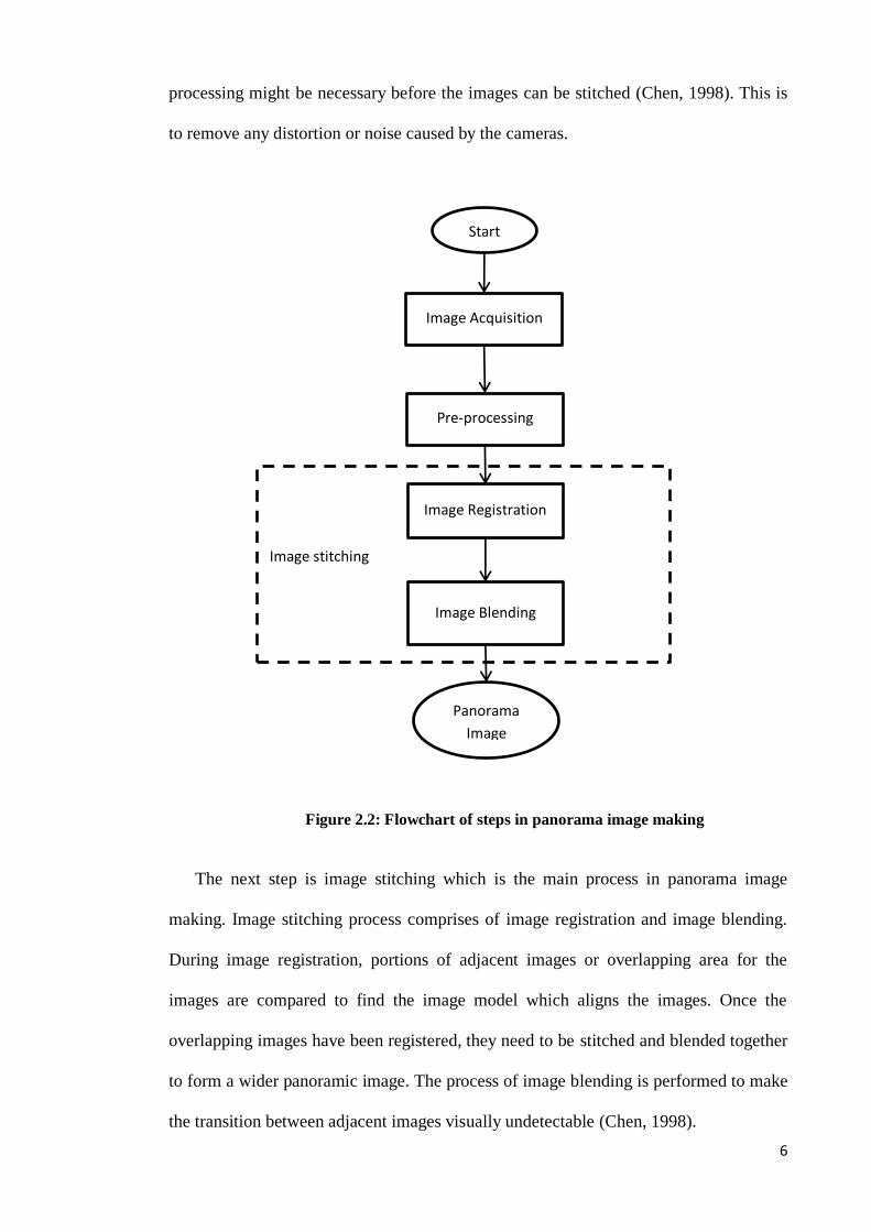
2.2 Panorama Image Making Process
Panoramic image making is the process of generating a bigger panoramic image by
combining a series of smaller, overlapping images (Chen, 1998). It consists of a
number of steps including image acquisition, pre-processing and image stitching.
Figure 2.1 shows the general flow of steps in the process.
The first step taken in the generation of a panoramic image is image acquisition.
Images can be taken from different sensors like cameras or from a single camera but
from different positions or angles. Once the images are digitized and stored, some pre-
6
Image stitching
Image Registration
Image Blending
Panorama
Image
Pre-processing
Start
Image Acquisition
processing might be necessary before the images can be stitched (Chen, 1998). This is
to remove any distortion or noise caused by the cameras.
Figure 2.2: Flowchart of steps in panorama image making
The next step is image stitching which is the main process in panorama image
making. Image stitching process comprises of image registration and image blending.
During image registration, portions of adjacent images or overlapping area for the
images are compared to find the image model which aligns the images. Once the
overlapping images have been registered, they need to be stitched and blended together
to form a wider panoramic image. The process of image blending is performed to make
the transition between adjacent images visually undetectable (Chen, 1998).

7
2.3 Image Acquisition
Image acquisition is the process of capturing the images. This can be taken from
different sensors such as camera, webcam or x-ray equipment. The objective of image
acquisition is to transform optical images into 2D arrays of numerical data which can
be manipulated by a computer (Awcock & Thomas, 1995). To create a panorama
image, each image acquired from the sensor should be partially overlapping with the
previous and the following images. It is desirable for the current image to have
sufficient overlapping area with the previous and the following images at least 30% of
overlapping area is recommended (Chen, 1998). The larger the overlapping region the
easier it is for adjacent images to be merged.
There are three common set-ups for image acquisition that can be used to capture
input images which will produce different types of panoramic images. In the first set-
up, the camera is set upon a tripod and the images are captured while rotating the
camera. The second set-up places the camera on a sliding plate and the images are
obtained by shifting the camera on a sliding plate. The third set-up is where the camera
is held in a person’s hands and the person takes the images by turning around on the
same spot, or walking in a direction perpendicular to the camera’s view direction
(Chen, 1998). However, images acquired by this method can be difficult to stitch, due
to the amount of unwanted camera rotation or translation during the acquisition of
images. Therefore, when taking images using portable handy camera, careful steps
must be taken to avoid distortion caused by hand movement.

8
2.4 Image pre-processing
Raw digital images acquired from sensors are usually corrupted by noise and other
undesirable effects such as occlusion and distortion. Thus, it might be necessary to
apply pre-processing procedures to clean these effects (da Fontoura Costa & Cesar,
2009). The aim of image preprocessing is to modify the pixel values of the digitized
images so that they are more suitable for subsequent operations in image processing
(Awcock & Thomas, 1995). The process of image pre-processing can be divided into
image enhancement and image restoration. Image enhancement attempts to improve the
quality or to emphasize certain aspects of the image. On the other hand, image
restoration aims to recover the original image after it has been corrupted by geometric
distortion within the camera system or blur caused by poor optic or movement. Both
types of operations take the acquired image array as input and produce an improved
modified image array as output (Awcock & Thomas, 1995).
Conventional image enhancement techniques include color conversion, histogram
conversion and color composition. Images can be categorized into color images and
grey-level images. Each pixel of the grey-level image has only one component value as
opposed to color images pixels; therefore, there have been many algorithms for contrast
enhancement that can be applied on grey-level images. On the other hand, since each
pixel of color images consists of color information as well as grey-level information,
these typical techniques for grey-level images cannot be applied to color images (Xiao
& Ohya, 2007). Thus, color conversion is usually necessary before applying any image
processing operation.
In color conversion, color information from one color space is converted to another.
The dominant colors in the visible portion of the light spectrum can be divided into
three component which are red, green and blue. These three colors are considered the

9
primary colors in the visible light spectrum. The RGB color space, in which color is
specified by the amount of Red, Green and Blue present in the color, is known as the
most popular color space (Xiao & Ohya, 2007). Pixels in the original color image can
be represented as the vector I(x, y) = [Ir (x, y) Ig (x, y) Ib(x, y)]T, where the r, g, and b
subscripts denote the red, green, and blue color planes, respectively (Gonzalez, Woods,
& Eddins).
Image restoration, is concerned with the reconstruction of the uncorrupted image
from a blurred and noisy one. An image restoration algorithm is different from image
enhancement methods in that they are based on models for the degrading process and
for the ideal image (Lagendijk & Biemond, 1999). Image restoration using linear
spatially invariant restoration filter can be modeled mathematically as follows.
g(n1,n2) = d(n1,n2)*f(n1,n2) + w(n1,n2)
where f(n1,n2) denotes the desired ideal spatially discrete image that does not contain
any blur or noise, d(n1,n2) is the blurring function, g(n1, n2 ) is the degraded image and
w(n1,n2) is the noise that corrupts the blurred image.
To remove noise or blur from an image, linear filter can be used. One example of
linear filter is an inverse filter. Inverse filter can be modeled mathematically as below
( ) ( ) ∑ ∑ ( )
( ) ( )
hinv(n1 , n2) is the inverse of the blurring function d(n1 , n2 ) and ( ) is an identity
matrix. Inverse filter has the advantages where it only requires blur point spread
function as a priori knowledge, and that it allows for perfect restoration in the case that
noise is absent (Lagendijk & Biemond, 1999).

10
2.5 Image Registration
The main process in panorama image stitching is registration. Image registration
can be defined as a process of overlaying two or more images of the same scene taken
at different times, from different viewpoints, and by different sensors (Zitova &
Flusser, 2003).In this thesis, the image registration process is limited to finding the
correct translation to align and merge adjacent images. More generally, in image
registration, portions of two adjacent or consecutive images are compared to find the
position and the needed transformation that will be used to combine the images
seamlessly. Image registration can be classified into direct method and feature based
method.
Direct based methods use pixel to pixel matching to maximize a measure of image
similarity between two sub-images and subsequently find a parametric transformation
to combine the two sub-images. Feature- based methods first extract salient features
such as corners from the two sub-images and then establish reliable feature
correspondences by comparing the features. Then images are warped according to
parametric transformations that are estimated from those correspondences (Feng,
2010). Direct methods have the advantage that they use all of the available image data
and hence can provide very accurate registration, but being iterative methods, they
require initialization. Unlike direct based methods, feature- based methods do not
require initialization but they are time consuming and for the majority of cases, finding
features in sub-images are difficult (Li & Ma, 2006). Some other methods can be
regarded as the combinations of the two above-mentioned methods (L. G. Brown,
1992; Chen, 1998; Zitova & Flusser, 2003).
Variants of image registration algorithm are used in many other applications such
as stereo vision and video compression schemes. Similar parametric motion estimation

11
algorithms have found a wide variety of applications, including video summarization,
medical imaging and remote sensing. For some previous surveys of image registration
techniques see (L. G. Brown, 1992; Chen, 1998; Zitova & Flusser, 2003).
2.5.1 Direct based method
Hoh et al. (Hoh, 1993) compared the SAD and SSD similarity measures for the
rigid registration of cardiac PET emission images. In the SAD method, registered
images are subtracted pixel-by-pixel, and the mean value of the sum of the absolute
intensity difference of all the pixels in the subtracted image is computed. Although the
two methods are similar, in the SSD the squared intensity difference is calculated
whereas in the SAD method the absolute difference is used. It is found that the SSD is
the optimum measure when registered images differ only by Gaussian noise,
(Fitzpatrick, 2000; Makela et al., 2002; Paul, 1997). In the paper, the effects of various
defects and misalignments were simulated. No significant differences in the translation
or rotation errors of the SAD and SSD algorithms were found.
Slomka et al. (P. J. Slomka, Gilbert, A. H., Stephenson, J., & Cradduck, T., 1995)
compared the SAD and SSC methods for affine registration of SPECT emission images
to templates. Slomka et al. (P. J. Slomka, Gilbert, A. H., Stephenson, J., & Cradduck,
T., 1995) found out that the SAD method provided better results than the SSC. This
method was later utilized for the quantification of SPECT images as a clinical tool (P.
J. slomka, Radau, P., Hurwitz, G. A.,Dey, D., 2001). The SSD-based similarity
measure has also been applied in rigid motion correction of gated heart perfusion MR
images (Bidaut, 2001).
Cross-Correlation is a basic statistical approach used as a similarity measure in
many image registration procedures. It is a match metric between two sub-images. This

12
similarity measure is widely used since it can be computed efficiently using the Fast
Fourier Transform (FFT) especially for combining large sub-images of the same size.
Furthermore, both direct correlation and correlation using FFT have costs which grow
at least linearly with the image area. Turkingston et al. (Turkington, 1997) utilized
cross-correlation measure for the rigid alignment of dynamic cardiac PET images to
cardiac templates. The method used only translations, assuming that the orientation of
the heart remains the same during the study.
The cross-correlation technique has also been proposed for rigid motion correction
of cardiac SPECT images (M. K. O’Connor, Kanal, K. M., Gebhard, M. W., &
Rossman, P. J. , 1998), (M. K. O’Connor, 2000). Bettinardi et al. (Bettinardi, 1993)
utilized the cross-correlation measure to rigidly register two PET transmission images
for patient repositioning. Cross-correlation measure was also used for the correction of
the patient motion in the PET heart studies with the help of PET transmission images,
taken before and after emission imaging (Bettinardi, 1993).
Kumar et al. (Kumar, 2010) proposed a method for stitching medical image using
histogram matching coupled with sum of squared difference to overcome the drawback
of feature based method for image alignment (Kumar, 2010). Although their method
improves the efficiency of the similarity measure and search, they still have increasing
complexity and the degrees of freedom of the transformation are increased.
Furthermore, hence the sum of squared difference method is not differentiable at the
origin; it is not well suited to gradient descent approaches.
Yu and Mingquan adopted the grid based registration method for the medical
infrared image (Y. Wang, & Wang, M. , 2010). They used the sum of squared
difference metric to measure similarity between the pixels in the two images. In order
to improve the registration accuracy and reducing the computational time; they divided
the registration process into two steps. The first step is rough registration, which

13
records the best registration point position, while the second step is precise registration.
When the current best registration point as the centre, the template moves n grids and
computes the square of difference of corresponding pixels in the two images (Y. Wang,
& Wang, M. , 2010). The processing time decreased slightly by using the two steps, but
still suffers from the complexity. An alternative to taking intensity differences is to
perform correlation, i.e., to maximize the product (or cross-correlation) of the two
aligned images.
Capek (Čapek, 2002) utilized the point matching method together with the
normalized correlation coefficient (NCC) to evaluate a similarity measure of X-ray
image. They claim that their method gave precise and correct results but the time taken
for processing is long (Čapek, 2002). The normalized cross-correlation (NCC) score is
always guaranteed to be in the range [−1, 1], which makes it easier to handle in some
higher-level applications (such as deciding which patches truly match). However, the
NCC score is undefined if either of the two patches has zero variance. In fact, its
performance degrades for noisy low-contrast regions.
Matsumoto et al. (T. Matsumoto, Takahashi, T., Iwahashi, M., Kimura, T., Salbiah,
S. & Mokhtar, N., 2011) use Phase Only Correlation (POC) based on Fast Fourier
Transform to generate panorama image of the ceiling (ceiling map) between two
adjacent frames in the video. Similarly, the location of another robot can be estimated
on the ceiling map by using a visual motion calculated from POC between the current
frame and the previously generated ceiling map. POC is only enough when the robot
move straight. When the robot makes a turn, panorama image cannot be match using
POC. Therefore, Rotation Invariant Phase only Correlation (RI-POC) is proposed to
match adjacent image which was rotated (T. Matsumoto, Takahashi, T., Iwahashi, M.,
Kimura, T., Salbiah, S. & Mokhtar, N., 2011). However, because of complexity,
RIPOC requires double computation to locate the robot. To cope with this problem, the

14
Functionally Layered Coding (FLC) was proposed (T. Matsumoto, Takahashi, T.,
Iwahashi, M., Kimura, T., Salbiah, S. & Mokhtar, N., 2010).
Savvides M. et al. (Savvides, Kumar, & Khosla, 2002) use Minimum Average
Correlation Energy (MACE) filter for face verification. A comparison of verification
performance between the correlation filter method and individual Eigenface Subspace
Method (IESM) shown that MACE filter offers significant potential for face
verification. Correlation method had the advantages include shift-invariant and ability
to suppress inposter faces using a universal threshold.
2.5.2 Feature based method
The development of image matching by using a set of local interest points can be
traced back to the work of (Moravec, 1981) on stereo matching using a corner detector.
The Moravec detector was improved by Harris and Stephens (Harris & Stephens, 1988)
to make it more repeatable under small image variations and near edges. Harris also
showed its value for efficient motion tracking and 3D structure from motion recovery
(Harris, 1993), and the Harris corner detector has since been widely used for many
other image matching tasks. While these feature detectors are usually called corner
detectors, they are not selecting just corners, but rather any image location that has
large gradients in all directions at a predetermined scale.
The initial applications were to stereo and short-range motion tracking, but the
approach was later extended to more difficult problems. (Zhang, Deriche, Faugeras, &
Luong, 1995) showed that it was possible to match Harris corners over a large image
range by using a correlation window around each corner to select likely matches.
Outliers were then removed by solving for a fundamental matrix describing the
geometric constraints between the two views of rigid scene and removing matches that

15
did not agree with the majority solution. At the same time, a similar approach was
developed by (Torr, 1995) for long-range motion matching, in which geometric
constraints were used to remove outliers for rigid objects moving within an image.
The ground-breaking work of (Schmid & Mohr, 1997) showed that invariant local
feature matching could be extended to general image recognition problems in which a
feature was matched against a large database of images. They also used Harris corners
to select interest points, but rather than matching with a correlation window, they used
a rotationally invariant descriptor of the local image region. This allowed features to be
matched under arbitrary orientation change between the two images. Furthermore, they
demonstrated that multiple feature matches could accomplish general recognition under
occlusion and clutter by identifying consistent clusters of matched features. The Harris
corner detector is very sensitive to changes in image scale, so it does not provide a
good basis for matching images of different sizes.
Lowe (D.G. Lowe, 1999) extended the local feature approach to achieve scale
invariance. This work also described a new local descriptor that provided more
distinctive features while being less sensitive to local image distortions such as 3D
viewpoint change.
Brown and Lowe (M. Brown, & Lowe, D.G., 2007) proposed a fully automated
panoramic image stitching using Scale Invariant Features Transform (SIFT) (D. G.
Lowe, 2004) to extract and match features between all of the images. From the features
matching step, image that have a large number of matches between them is identify.
Random Sample Consensus (RANSAC) is use to select a set of inliers that are
compatible with a homography between the images. Next, a probabilistic model is
applied to verify the match. Bundle adjustment is use after that to solve for all of the
camera parameters jointly. By applying a global rotation such that up-vectors u is
vertical (in the rendering frame) effectively removes the wavy effect from output

16
panoramas. Brown and Lowe had successfully matched multiple panoramas in
unordered image set and stitch them fully automatically without user input (M. Brown,
& Lowe, D.G., 2007).
Lepetit and Fua (Lepetit & Fua, 2004) introduced a simplified orientation
correction technique for real-time applications. The method only considers intensity
changes along a fixed-size circular region centred on each key-point. It is not, however,
robust to scale changes or out-of-plane rotations. The rotation invariance of their
proposed system still comes primarily from the multiple view training. Later Lepetit
and Fua (Lepetit & Fua, 2006) in their experimental results indicate a large number of
training views are crucial to the system’s reliability. However, even the affine
transformation space for simple planar objects has six parameters and thus demands a
huge number of training views for stable and reliable performance. For example, if only
100 features are kept for each object, then 1000 training views will generate 100,000
feature vectors per object. Consequently, proper feature selection is crucial for fast and
accurate performance of the whole system (Q. Wang & You, 2008).
Wang and You (Q. Wang & You, 2008) claims that although SIFT method (D. G.
Lowe, 2004) robust to image rotation and noise, but they are typically too
computationally expensive to be a component of real time image matching systems,
because the process generally involves time-consuming steps such as relative scale
searching, dominant orientation calculation, and pixel values extraction from irregular
regions (Q. Wang & You, 2008). (Q. Wang & You, 2008) propose a different approach
combining feature selection and multiple-view training into one unified framework to
enhance rotation invariance in real-time image matching system. First a small number
of rotation-dominant views are constructed to obtain a set of descriptors for each view
track. Then for those feature points with a high repeatability, raw ranking scores (RRS)
are calculated based on feature distinctiveness and invariance. Finally, the raw ranking
17
score is rescaled, weighted and combined with the other traditional feature selection
criterion for the final ranking score (FRS). Features with high FRS are selected.
Steedly (Steedly, 2005) used SIFT features to automatically and efficiently register
and stitch thousands of video frames into a large panoramic mosaic. To reduce the cost
of searching for matches between video frames by adaptively identifying key frames
based on the amount of image-to-image overlap. Key frames are matched to all other
key frames, but intermediate video frames are only matched to temporally
neighbouring key frames and intermediate frames. Image orientations can be estimated
from this sparse set of matches in time quadratic to cubic in the number of key frames
but only linear in the number of intermediate frames. Additionally, the matches
between pairs of images are compressed by replacing measurements within small
windows in the image with a single representative measurement.
Lee (Lee, 2005) use the corner points for the corresponding features, and
morphological structures were used for fast and robust corner detection. (Lee, 2005)
used the criterion of the corner strength, which guarantees the robust detection of the
corner in most situations. For the transformation, 8 parameters were estimated from
perspective equations, and bilinear colour blending was used to construct a seamless
panoramic video. From this experiments, the proposed method yields fast results with
good quality under various conditions.
Zheng (Zheng, 1992), proposed a dynamically generated panoramic representation
for route recognition by an autonomous mobile robot. The continuous panoramic view
(PV) and generalized panoramic view (GPV) were built by using dynamic
programming and circular dynamic programming employing feature matching in fine
verification. PV and GPV give the advantages of wide fields which brings a reliable
result to the scene recognition.

18
Li and Ma (Li & Ma, 2006) use two stage feature-based robust estimation which
quickly searches for a small number of consistent matches defining a transformation
that is well approximation to the correct one. After getting all matching pairs,
geometric relations of neighbouring points are used to eliminate the false matches, and
then Levenberg-Marquardt’s nonlinear method is used to minimize the differences and
update the related transformations. This paper used a coarse-to-fine method to construct
mosaics. Panorama blending with two band blending method gains high quality to
overcome large lighting variation between the images.
2.6 Image Blending
Image blending is the process of adjusting the values of pixels in two registered
images, such that when the images are matched, the transition from one image to the
next is seamless and at the same time the merging images should preserve the quality of
the input images as much as possible (Chen, 1998). Image blending is needed to
compensate for exposure differences and other misalignments (Szeliski, 2006).
Due to various reasons such as lighting condition and the geometry of the camera
set-up, the overlapping regions of adjacent images are almost never the same.
Therefore, removing part of the overlapping regions in adjacent images and
concatenating the trimmed images often produce images with distinctive seams. A
seam is the artificial edge produced by the intensity differences of pixels immediately
next to where the images are joined (Chen, 1998). (M. Brown & Lowe, 2003) used
multi-band blending in panorama creating. They use 2 band schemes where a low pass
image is formed with spatial frequency of wavelength greater than 2 pixels relative to
the rendered image and a high pass image with spatial frequencies less than 2 pixels.

19
Low frequency information is then blend using a linear weighted sum, and high
frequency information for image is selected with the maximum weight.
Xiong and Pulli (Xiong & Pulli, 2010) claims that transition smoothing approaches
will reduce color differences between sources images to make seams invisible and
remove stitching artifacts. It can be divided into two method which is alpha blending
and gradient domain image blending. Alpha blending is widely used and fast transition
smoothing approach but it cannot avoid ghosting problems caused by object motion
and spatial alignment errors. Gradient domain image blending approaches can reduce
color differences and smooth color transitions to produce high-quality composite
images.
Xiong and Pulli (Xiong & Pulli, 2010) use a simple linear blending when source
images are similar in color and luminance but when the colors remain too different,
Poisson blending hides visible seams. The use of color correction for the source images
can improve qualities of image labeling and image blending. It can also speed up the
blending process.
Rankow et.al (Rankov, Locke, Edens, Barber, & Vojnovic, 2005) uses gradient
method for blending a mosaic image of tumor for clinical studies. They claim that this
method can used to eliminates sharp intensity changes at the image joins. Blending was
done by separating color planes, where necessary, applying blending algorithm for each
color band and recomposing planes together to get full color image at the output.
Hu (W.C. Hu, 2007) proposed blending method in a two-phase scheme which is the
histogram-based blending is first applied in the first phase scheme, and then in the
second phase scheme, the weighted blending is used under the result of the first phase
scheme. They proved that the performance of the proposed blending method is better
than the three basic blending schemes (the weighted blending, the adaptive blending,
and the histogram-based blending).

20
2.7 Summary
In this chapter, a literature survey on the components of a panorama image making
is presented. The focus of the survey is on the image stitching which is the most
important component in panorama creation. Existing methods for image stitching
algorithm are reviewed and categorized into direct based and feature based methods.
Some popular direct based methods are discussed and similarly a review of some well-
known feature based methods is included. Finally, several popular image blending
methods are examined.

21
Chapter 3
Methodology
3.1 Chapter Overview
One of the simplest forms of correlation filters is known as the matched spatial
filter (MSF) (Čapek, 2002; Kumar, 2010). It performs well at detecting a reference
image corrupted by additive white noise but this technique suffers from distortion
variance, poor generalization and poor localization properties. The reason for this poor
performance is because MSF uses a single training filter to generate broad correlation
peaks (Lee, 2005). This shortcoming is addressed by introducing another correlation
filter that is known as a synthetic discriminant function (SDF). It is a linear
combination of MSFs. It linearly combines a set of training images into one filter which
further allows users to constrain the filter output at the origin of the correlation filter
(Zheng, 1992). These pre-specified constraints are known as ‘peak constraints’. SDF
filters provide some degree of distortion in variance but like MSFs they result in large
side-lobes and broad correlation peaks that make localization difficult.
To reduce large side-lobes observed in SDFs and to maximize peak sharpness for
better object localization and detection, MACE (minimum average correlation energy)
filters were introduced. A MACE filter can be obtained from the FFT of a single
training image or synthesized from the FFTs of a few training images. When the FFT
of a test image is presented, a 2D correlation plane is computed and a sharp correlation
peak is observed at the position that produces the maximum correlation between the
test image and the training image (da Fontoura Costa & Cesar, 2009; Steedly, 2005;
Szeliski, 2006).

22
For image stitching, the correlation values are very close to zero for all points
except at the location where the two sub-images match. Exploiting this simple attribute
of the MACE filter, a stitching approach based on pattern correlation (PCB) is
developed and its details are presented in the following sections. The proposed system
employs correlation filters to find the best matched position for two x-ray images that
are combined to form a single image.
In this chapter a method for image stitching is proposed along with the steps
required to implement the proposed approach. The pattern matching approach is based
on Minimum Average Correlation Energy (MACE) filter. Further details are discussed
in subsequent sections.
3.2 Correlation measurement
Correlation provides the measure of similarity between two signals. In the time
domain, the correlation of signal g and h is represented by equation (1).
( ) ∫ ( ) ( )
(1)
In the frequency domain, the correlation of signals g and h can be computed by
multiplying the Fourier transform of one of them to the complex conjugate of the
Fourier transform of the other.
( ) ( ) ( ) (2)
The following diagram shows the configuration of the frequency domain correlation
operation where the Fourier transform of signal g is multiplied to the complex
conjugate of the Fourier transform of signal h.
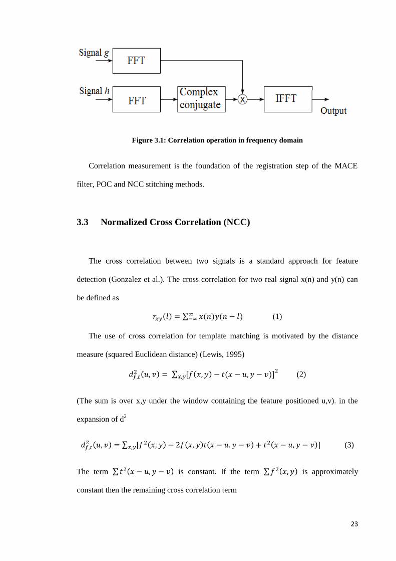
23
Figure 3.1: Correlation operation in frequency domain
Correlation measurement is the foundation of the registration step of the MACE
filter, POC and NCC stitching methods.
3.3 Normalized Cross Correlation (NCC)
The cross correlation between two signals is a standard approach for feature
detection (Gonzalez et al.). The cross correlation for two real signal x(n) and y(n) can
be defined as
( ) ∑ ( ) ( ) (1)
The use of cross correlation for template matching is motivated by the distance
measure (squared Euclidean distance) (Lewis, 1995)
( ) ∑ ( ) ( )
(2)
(The sum is over x,y under the window containing the feature positioned u,v). in the
expansion of d2
( ) ∑ ( ) ( ) ( ) ( ) (3)
The term ∑ ( ) is constant. If the term ∑ ( ) is approximately
constant then the remaining cross correlation term

24
( ) ∑ ( ) ( ) (4)
is a measure of the similarity between the image and the feature. If the image energy
∑ ( ) is not constant however, feature matching by cross correlation can fail.
Normalized cross correlation overcomes these difficulties by normalizing the image
and template vectors to unit length, yielding a cosine-like correlation coefficient
( ) ∑ [ ( ) ] ( )
√{∑ [ ( ) ] ( ) }
(5)
Where is the mean of the template and is the mean of f(x,y) in the region
under the feature (Lewis, 1995). Consider the numerator in (1) and assume that we
have images ( ) ( ) and ( ) ( ) in which the mean
value has already been removed:
( ) ∑ ( ) ( ) (6)
Equation (2) above is a convolution of the image with the reversed template ( )
and can be computed by
{ ( ) ( )} (7)
Where is the Fourier transform. The complex conjugate accomplishes reversal of
the template via the Fourier transform property ( ) ( ). The desired
position of image matching of the pattern is equivalent to the position ( ) of
the maximum value in of ( ).

25
3.4 Phase only Correlation
In general both the magnitude and the phase are needed to completely describe a
function in the frequency domain. Sometimes, only information regarding the
magnitudes is displayed, such as in the power spectrum, where phase information is
completely discarded. However when the relative roles played by the phase and the
magnitude in the Fourier domain are examined, it is found that the phase information is
considerably more important than the magnitude in preserving the features of an image
pattern.
The Fourier synthesis using full-magnitude information with a uniform phase
resulted in nothing meaningful as compared to the original images. Inspired by the
above findings, investigations of the use of phase-only information for matched filters
or pattern recognition have been carried out. It is found that the phase only approach
produces a sharp correlation peak.
Consider two n1 x n2 images, f(n1 , n2 ) and g(n1 , n2 ) where we assume that the
index range are n1 =-M1.…….M1(M1>0) and n2=-M2.….M2(M2>0) for mathematical
simplicity, and hence n1=2 x M1+1 and n2=2 x m2+1 (Ito, Aoki, Nakajima, Kobayashi,
& Higuchi, 2006). Let F(k1,k2) and G(k1,k2) denote the two dimension discrete Fourier
transforms (2D DFT) of the two images. F(k1,k2) and G(k1,k2) are given by
F(k1,k2) = ∑ ( )
= ( ) ( ) (1)
G(k1,k2) = ∑ ( )
= ( ) ( ) (2)

26
Where k1 = -M1 … M1 , k2 = -M2 … M2 , (
)
(
) and the operator ∑n1,n2 denotes ∑
∑
( ) and ( ) are amplitude components and ( ) and ( )
are phase components. The cross spectrum RFG (k1,k2) between F(k1,k2) and G(k1,k2) is
given by
RFG(k1,k2) = F(k1,k2) ( )
= AF(k1,k2)AG(k1,k2) ( ) (3)
Where ( ) denotes the complex conjugate of G( ) and ( ) denotes
the phase difference ( ) ( ). The ordinary correlation function is
given by the two dimension inverse discrete Fourier transform (IDFT) of ( )
and is given by
( )
∑
( )
(4)
Is the 2D inverse Fourier transforms of ( )
Where∑ ∑
∑
. On the other hand, the cross phase
spectrum ( ) is defined as
( ) ( ) ( )
| ( ) ( ) |
= ( ) (5)

27
The phase only correlation (POC) function ( ) is the 2D IDFT of ( )
and is given by
( )
∑ ( )
(6)
When ( ) and ( ) are the same image, i.e, ( ) ( ), the POC
function will be given by
( )
∑
= ( )
= {
(7)
The equation (1) implies that the POC function between two identical images is the
kronecker’s delta function ( ).
3.5 Proposed approach for image stitching system
The proposed approach consists of four steps and they are listed below.
(i) Image pre-processing
(ii) Fourier transformation and MACE filter design
(iii) Inverse transformation, peak and PSR measurements
(iv) Image blending
The proposed PCB (pattern correlation based) image stitching system is shown in
Figure 3.2. It consists of pre-processing; Fourier transformation and MACE filter

28
design, inverse transformation, peak and Peak to Sidelobe Ratio (PSR) measurement
and image blending. In the forthcoming sections, details of each step are discussed.
Image Preprocessing
Image Processing Strategy
MACE Filter Designing
Time Domain
Transformation
Finding Peak Value
Calculating Peak to
sidelobe Ratio
Step 1
Step 2
Step 3
Panoramic Image
Creating Technique
Creating seem less
panorama
Image Stitching
Step 4
Frequency
Domain
Transformation
Correlation
Transformation
Figure 3.2: Proposed Image Stitching Method
3.6 Image pre-processing
Image pre-processing is the first step needed to prepare the image. In this thesis, the
proposed method will be performed using grey-level images. Therefore, if the inputs
are color images they will undergo color conversion to grey scale. This is followed by
histogram equalization to remove intensity variations caused by external factors such as
uneven illumination. Then windowing is performed using Hanning window before
Fourier transformation to avoid leakage in the signal caused by its energy smearing out

29
over a wide frequency range in the FFT. After that FFT is performed on the pre-
processed images.
3.6.1 Colour to grey scale conversion
The first step of the proposed method is color to greyscale conversion. Since images
from the databases are all in RGB, color conversion is needed before further
processing. To convert the RGB values to single grayscale intensity, the following
formula is used
Intensity = 0.2989*red + 0.5870*green + 0.1140*blue
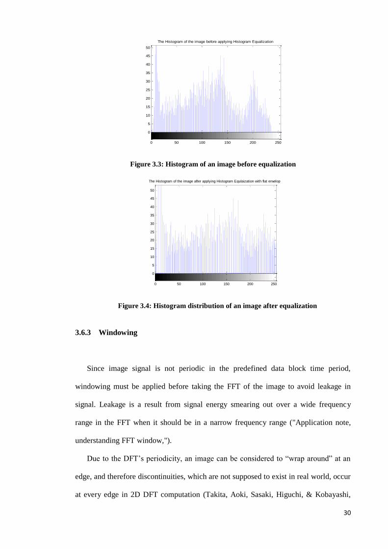
3.6.2 Histogram Equalization
Intensities in the images are highly sensitive to external factors such as, illumination,
reflection, and lighting variation. These external factors affect the distribution of
intensities in the histogram of the images ("Application note, understanding FFT
window,"), which in turn might affect the accuracy of the ensuing process if left
uncorrected. In order to remove the influence of particular contrast and brightness on
the intensity of the images, histogram equalization can be applied on the images to re-
distribute the intensities throughout the range.
Let f be a given image represented by row and column matrix of integer pixel
intensities ranging from 0 to L-1. L is the number of possible intensity values, usually 256. Let
p denote the normalized histogram of f with a bin for each possible intensity given as;
Where n=0,1…..,L-1.
30
Figure 3.3: Histogram of an image before equalization
Figure 3.4: Histogram distribution of an image after equalization
3.6.3 Windowing
Since image signal is not periodic in the predefined data block time period,
windowing must be applied before taking the FFT of the image to avoid leakage in
signal. Leakage is a result from signal energy smearing out over a wide frequency
range in the FFT when it should be in a narrow frequency range ("Application note,
understanding FFT window,").
Due to the DFT’s periodicity, an image can be considered to “wrap around” at an
edge, and therefore discontinuities, which are not supposed to exist in real world, occur
at every edge in 2D DFT computation (Takita, Aoki, Sasaki, Higuchi, & Kobayashi,
0 50 100 150 200 250
0
5
10
15
20
25
30
35
40
45
50
The Histogram of the image before applying Histogram Equalization
0 50 100 150 200 250
0
5
10
15
20
25
30
35
40
45
50
The Histogram of the image after applying Histogram Equlaization with flat envelop

31
2003). To reduce the effect of discontinuity at image border, 2D Hanning window
function is applied to the input images. Hanning window is chosen since it does not
suddenly cut off the signal at its edges, but rather rolls off smoothly towards the edge.
3.6.4 Fourier transformation and MACE filter design
The Discrete Fourier Transform (DFT) is a mathematical operation that converts
function in time domain into frequency domain. When stitching two images, out of the
two input images only one is needed to construct the MACE filter. First, Fourier
transformation is performed on both images using the Fast Fourier Transform (FFT).
The two images can be regarded as two dimensional (2D) signals f(n1, n2) and g(n1,
n2)and their Fourier transform coefficients are F(k1,k2) and G(k1,k2) given by Equations
1 and 2 respectively.
( 1 2) ∑ ( )
( ) ( ) (1)
( 1 2) ∑ ( )
( ) ( ) (2)
where k1 = -M1 … M1,k2= -M2 … M2, (
)
(
).
If f(n1, n2) is the image chosen to construct the filter, the MACE filter equation
becomes
( 1 2) ( )
( ) ( 1 ) (3)

32
where MACE represents the MACE filter, F(K1, K2) is the FFT transformed image and
‘ ( ) ’ represents the complex conjugate of F(K1, K2). The flowchart of image
stitching algorithms is shown in figure 3.5.
The correlation between the MACE filter and the second image is then measured as
follows.
( ) (( ( 1 2) ) ( 1 2)) (4)
Where ( ) represents the complex conjugate of G(K1, K2).
Image Database
Frequency Domain
Transformation
First Image in Frequency
Domain
MACE Filter
Construction
Correlation Calculation
Time Domain
Transformation
Second Image in Frequency
Domain
Peak and PSR
calculation
First
image
second
image
Image Blending
Figure 3.5: Flowchart of the proposed method

33
3.7 Inverse Transformation, peak and PSR measurements
Since the correlation is measured in frequency domain, it has to be inverse
transformed so that the relative values of correlation at various positions can be
observed. The inverse Fourier transform of the correlation function is given by
Equation 5
( )
∑ ( )
(5)
The values of cfg (n1, n2) are stored in a 2D correlation plane where the absolute
value and location of the highest peak are identified. This position gives the highest
correlation between the two input images. To ensure that the two images are indeed
overlapping, the Peak to Sidelobe Ratio (PSR) is calculated using the location of the
highest peak.
It is observed that the correlation plane for two non-overlapping images is devoid of
a dominant peak but contains many non-dominant local peaks. The dominance of the
highest peak is related to the value of the PSR. Therefore, it can be used as an indicator
of the peak dominance and a threshold can be set to separate dominant peak of
overlapping images from non-dominant peak of non-overlapping images. By trial and
error, the threshold for the PSR value in the following experiments is set at 15. If the
PSR of a pair of matched images is less than 15, the system classifies those images as
not overlapping.
The PSR is defined as
–
(6)
Where μ and σ are the mean and standard deviation of the sidelobe region
respectively. In our experiment, the area occupied by the peak is estimated to be 5x5 as

34
indicated by the blue rectangle in Figure 3.6. Thus, the mean and standard deviation of
the sidelobe region must be calculated outside of the 5x5 peak area in a 20x20 region.
The 20x20 area encloses the 5x5 peak area at its centre.
Figure 3.6: The area of the peak and PSR
3.8 Image blending
Once the PSR value is calculated, it will decide whether the image is overlapping or
not overlapping. If the value of PSR is higher than the threshold value, the image is
considered overlapping and panorama image will be created by blending the input
images based on the location of peak value. Otherwise the input images are considered
not overlapping and no further action is taken.
In image blending, information from the location of the Peak of the correlation
plane is used to translate the images to the right position before merging them. Then the
intensities of pixels at the borderline between the two images are adjusted so that the
transition from one image to the next is smooth. In our image stitching system we
employ alpha blending to adjust the local pixel intensity around the borderline area.
Sidelobe Region
Peak
5 x 5 mask
35
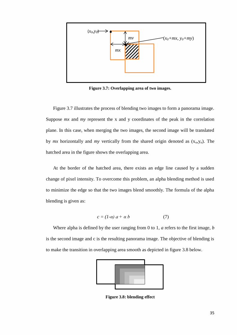
Figure 3.7: Overlapping area of two images.
Figure 3.7 illustrates the process of blending two images to form a panorama image.
Suppose mx and my represent the x and y coordinates of the peak in the correlation
plane. In this case, when merging the two images, the second image will be translated
by mx horizontally and my vertically from the shared origin denoted as (xo,yo). The
hatched area in the figure shows the overlapping area.
At the border of the hatched area, there exists an edge line caused by a sudden
change of pixel intensity. To overcome this problem, an alpha blending method is used
to minimize the edge so that the two images blend smoothly. The formula of the alpha
blending is given as:
c = (1-α) a + α b (7)
Where alpha is defined by the user ranging from 0 to 1, a refers to the first image, b
is the second image and c is the resulting panorama image. The objective of blending is
to make the transition in overlapping area smooth as depicted in figure 3.8 below.
Figure 3.8: blending effect
(x0+mx, y0+my) my
mx
(x0,y0)

36
3.9 Performance Evaluation
The relative performances of the methods are measured by four parameters that
represent accuracy and they are True Positive Rate (TPR), False Positive Rate (FPR),
True Negative Rate (TNR), and False Negative Rate (FNR). TPR is the ratio of the
number of overlapping images detected by the system to the total number of
overlapping images. In contrast, FPR is the ratio of the number of non-overlapping
images confirmed by the system to the total number of non-overlapping images. FNR
and TNR are the complements of TPR and FPR respectively. They are expressed by the
equations 8, 9, 10 and 11 as follow;
(8)
(9)
FNR = 100% - TPR (10)
TNR = 100% - FPR (11)
Another performance index that indicates the efficiency of the proposed method is
the execution time. Besides accuracy, the execution time of the proposed method is also
compared to those of the normalized correlation coefficient (NCC) and Phase Only
Correlation (POC) methods.

37
3.10 Summary
In this chapter, the overall strategy of the proposed method, its steps and algorithms
are described. Details of pre-processing, Fourier transformation, MACE filter design,
inverse transformation, peak and Peak to Sidelobe Ratio (PSR) measurement and image
blending are presented. The rationales of implementing the steps along with the
explanation on terms are used to measure the performance of the method are
elaborated. Now the method will be tested to recognize overlapping images and then
used to stitch them in the next chapter.

38
Chapter 4
Image Stitching of Radiographic Images
4.1 Introduction
Normally, x-ray images are captured using special cassettes and films of limited size
since conventional x-ray equipment can only provide a limited visual field. However,
in some cases using one x-ray image is not enough to detect any abnormality in human
body. Therefore, to construct higher resolution and larger images from the conventional
x-ray images, image stitching methods such as the one proposed in chapter 3 can be
utilized. In this chapter, the ability of the proposed method to stitch radiographic
images is tested. The performance of this method and those of the NCC and POC
methods are explored in a few experiments conducted using three different databases.
Both the rates of accuracy and execution time of the MACE filter, NCC and POC are
compared and summarized.
4.2 Image databases
Three sets of databases were used in the experiments and they contain the x-ray
images of spine, scoliosis and hand. There are 20 pairs of overlapping and 20 pairs of
non-overlapping spine images in the first database. Likewise, the second database
consists of 20 pairs of overlapping and 20 pairs of non-overlapping scoliosis images.
The third database contains 40 pairs overlapping and 40 pairs of non-overlapping hand
images. These radiographic images are secured from the medical faculty of King Fahd
University Hospital and open access databases of X-ray images from the internet.
39
The proposed algorithm is implemented in MATLAB 7.4 running on a computer
with 2.0GHz dual core OPTERON processor and 1.87GB RAM.
4.3 Spine image stitching
Spine functions to support weight and ties our body together. The spinal column
consists of a stack of small bones that range in size from 2-3 inches to 5-6 inches in
diameter. X-ray imaging is an important procedure to diagnose injury or deformation to
spine. Spine x-ray can be taken separately in 3 main parts which is on the neck
(cervical), mid back (thoracic), and lower back (lumbar). To produce the whole spine
image, digitized images from the three different parts can be assembled by stitching.
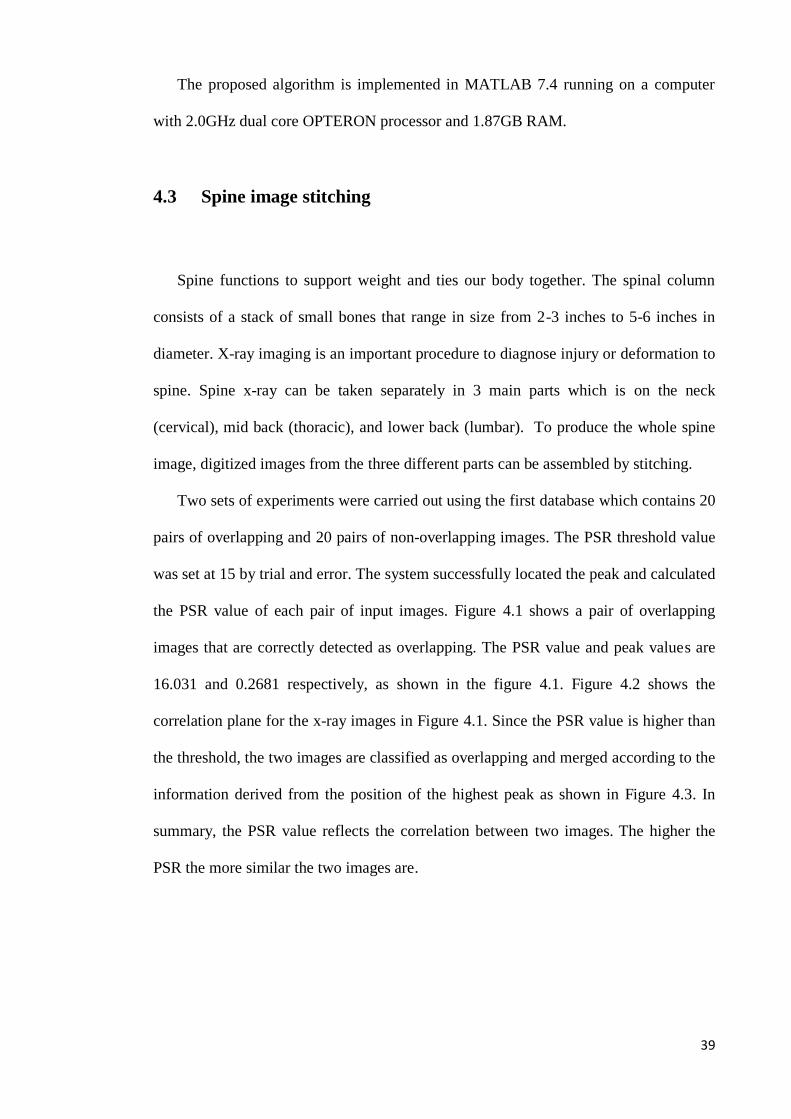
Two sets of experiments were carried out using the first database which contains 20
pairs of overlapping and 20 pairs of non-overlapping images. The PSR threshold value
was set at 15 by trial and error. The system successfully located the peak and calculated
the PSR value of each pair of input images. Figure 4.1 shows a pair of overlapping
images that are correctly detected as overlapping. The PSR value and peak values are
16.031 and 0.2681 respectively, as shown in the figure 4.1. Figure 4.2 shows the
correlation plane for the x-ray images in Figure 4.1. Since the PSR value is higher than
the threshold, the two images are classified as overlapping and merged according to the
information derived from the position of the highest peak as shown in Figure 4.3. In
summary, the PSR value reflects the correlation between two images. The higher the
PSR the more similar the two images are.

40
Figure 4.1: A pair of overlapping Images with Peak and PSR value.
Figure 4.2: Correlation Plane for images in figure 4.1

41
Figure 4.3: Blended Image for images in figure 4.1
Another pair of overlapping test images is shown in Figure 4.4. The correlation
plane and the final merged image are shown in Figures 4.5 and 4.6 respectively. Out of
20 pairs of overlapping images, 19 were detected and matched correctly. 1 pair of
overlapping images were detected as overlapping but not matched correctly.
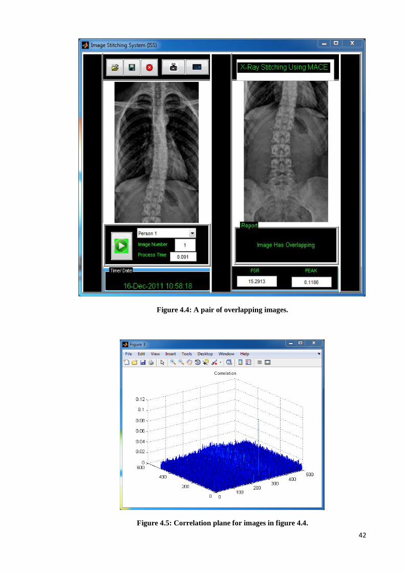
42
Figure 4.4: A pair of overlapping images.
Figure 4.5: Correlation plane for images in figure 4.4.

43
Figure 4.6 blended image for images in figure 4.4.
In the second set of experiments, 20 non-overlapping images were presented to the
system. The system ruled that all these images were uncorrelated since their PSR
values were lower than the threshold. An example of a pair of non-overlapping images
is shown in Figure 4.7. Figure 4.8 shows the correlation plane of these images. As

44
observed, there is no dominant peak in the correlation plane which results in a PSR
lower than the threshold. Further observation of Figure 4.8 reveals that besides the
highest peak there are a few high local peaks in the correlation plane.
Figure 4.7: A pair of non-overlapping images

45
Figure 4.8: Correlation plane for images in figure 4.7.
The performance of the proposed method is compared against those of the NCC and
POC methods using the same database. The relative performances of the methods are
measured by four quantities namely True Positive Rate (TPR), False Positive Rate
(FPR), True Negative Rate (TNR), and False Negative Rate (FNR) as described earlier.
The performance comparison is summarized in Table 4.1.
Table 4.1: Results of matching pairs of overlapping images using (TPR) and (FNR) Rates
Methods Total number
of overlapping
images
No. of overlapping
images correctly
identified and
stitche
TPR (%) FNR (%) Average
processing
time
(second)
Proposed 20 19 95% 5% 0.1
NCC 20 18 90% 10% 0.5
POC 20 18 90% 10% 0.2
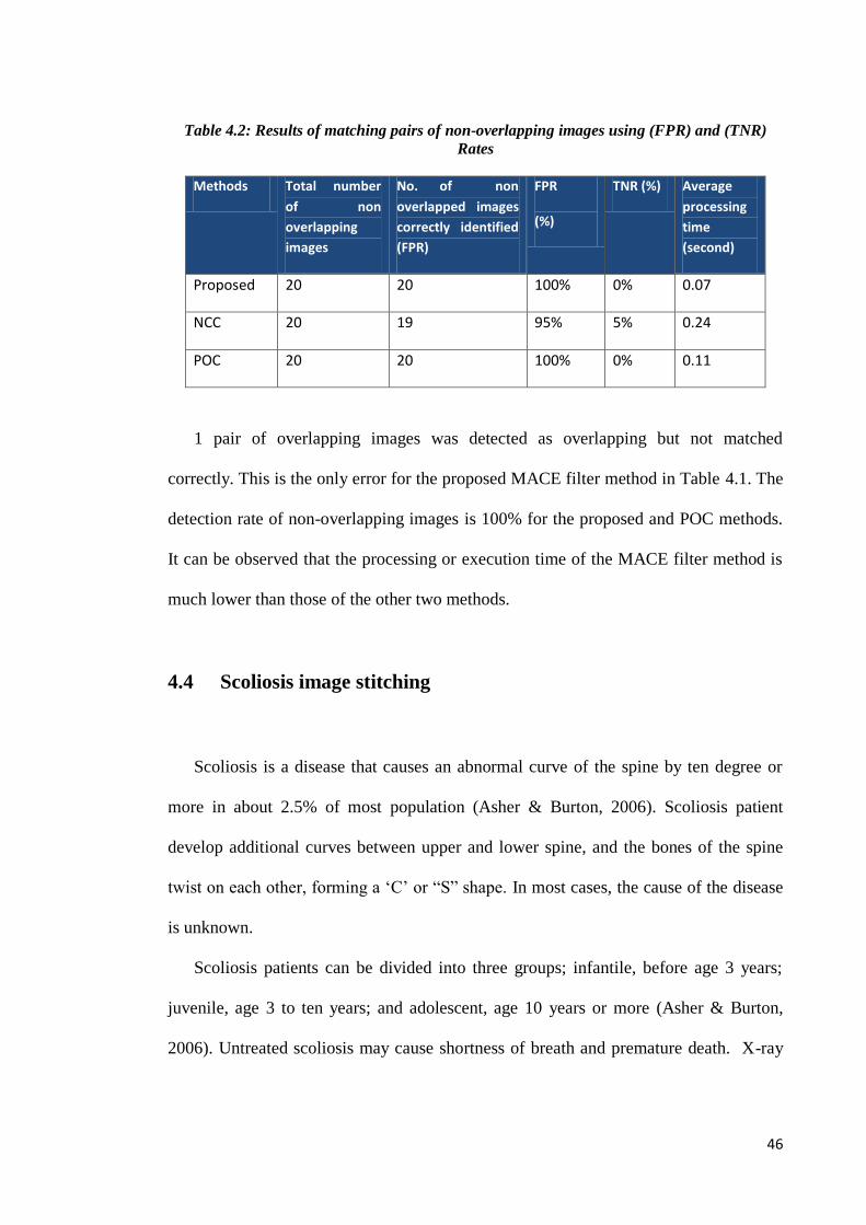
46
Table 4.2: Results of matching pairs of non-overlapping images using (FPR) and (TNR)
Rates
Methods Total number
of non
overlapping
images
No. of non
overlapped images
correctly identified
(FPR)
FPR
(%)
TNR (%) Average
processing
time
(second)
Proposed 20 20 100% 0% 0.07
NCC 20 19 95% 5% 0.24
POC 20 20 100% 0% 0.11
1 pair of overlapping images was detected as overlapping but not matched
correctly. This is the only error for the proposed MACE filter method in Table 4.1. The
detection rate of non-overlapping images is 100% for the proposed and POC methods.
It can be observed that the processing or execution time of the MACE filter method is
much lower than those of the other two methods.
4.4 Scoliosis image stitching
Scoliosis is a disease that causes an abnormal curve of the spine by ten degree or
more in about 2.5% of most population (Asher & Burton, 2006). Scoliosis patient
develop additional curves between upper and lower spine, and the bones of the spine
twist on each other, forming a ‘C’ or “S” shape. In most cases, the cause of the disease
is unknown.
Scoliosis patients can be divided into three groups; infantile, before age 3 years;
juvenile, age 3 to ten years; and adolescent, age 10 years or more (Asher & Burton,
2006). Untreated scoliosis may cause shortness of breath and premature death. X-ray

47
image of the spine is taken to measure and quantify the seriousness of the disease
before further treatment.
Depending on the degree of the curvature and whether it gets worse over time, the
doctor may recommend surgery. If the curve is less than 25°, no treatment is required,
and the sufferer should be reexamined every four to six months. If the curve is more
than 25° but less than 30°, a back brace may be used for treatment. Curves that are
more than 45° will need to be evaluated for the possibility of surgical correction.
Surgical correction involves fusing vertebrae together to correct the curvature and may
require inserting rods next to the spine to reinforce the spine.
When presented with a pair of scoliosis images, the tested methods would
determine whether the two images were overlapping. All of them would measure the
peak value and calculate the PSR. If the PSR was bigger than 15, the images would be
classified as overlapping. Figure 4.9 show a pair of overlapping scoliosis images and
Figure 4.10 shows their correlation plane. Since their PSR value is greater than 15, they
are stitched into a single image as depicted by Figure 4.11. Figures 4.12, 4.13 and 4.14
show another pair of overlapping scoliosis images, their correlation plane and stitched
image respectively. Finally, figures 4.15, and 4.16 show a pair of non-overlapping
scoliosis images and their respective correlation plane.
The results of the experiments with the second database involving overlapping and
non-overlapping scoliosis images are summarized in Table 4.3 and 4.4 respectively.
For overlapping scoliosis images, the PSR of one pair of images is lower than the
threshold value for the MACE filter approach. The other two approaches record 3
similar cases. For non-overlapping scoliosis images, the proposed MACE filter and
POC approaches record perfect accuracy while the NCC approach misclassifies only
one pair of images.

48
Figure 4.9: A pair of overlapping scoliosis images with calculated peak and PSR values.
Figure 4.10: Correlation plane for images in figure 4.9

49
Figure 4.11: Stitched image for images in figure 4.9
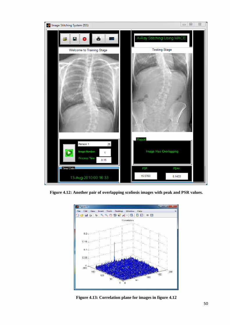
50
Figure 4.12: Another pair of overlapping scoliosis images with peak and PSR values.
Figure 4.13: Correlation plane for images in figure 4.12

51
Figure 4.14: Merged image for images in figure 4.12

52
Figure 4.15: A pair of non-overlapping scoliosis images with lower peak and PSR values.
Figure 4.16: Correlation plane for non-overlapping images in figure 4.15
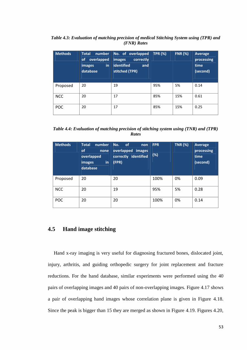
53
Table 4.3: Evaluation of matching precision of medical Stitching System using (TPR) and
(FNR) Rates
Methods Total number
of overlapped
images in
database
No. of overlapped
images correctly
identified and
stitched (TPR)
TPR (%) FNR (%) Average
processing
time
(second)
Proposed 20 19 95% 5% 0.14
NCC 20 17 85% 15% 0.61
POC 20 17 85% 15% 0.25
Table 4.4: Evaluation of matching precision of stitching system using (TNR) and (TPR)
Rates
Methods Total number
of none
overlapped
images in
database
No. of non
overlapped images
correctly identified
(FPR)
FPR
(%)
TNR (%) Average
processing
time
(second)
Proposed 20 20 100% 0% 0.09
NCC 20 19 95% 5% 0.28
POC 20 20 100% 0% 0.14
4.5 Hand image stitching
Hand x-ray imaging is very useful for diagnosing fractured bones, dislocated joint,
injury, arthritis, and guiding orthopedic surgery for joint replacement and fracture
reductions. For the hand database, similar experiments were performed using the 40
pairs of overlapping images and 40 pairs of non-overlapping images. Figure 4.17 shows
a pair of overlapping hand images whose correlation plane is given in Figure 4.18.
Since the peak is bigger than 15 they are merged as shown in Figure 4.19. Figures 4.20,
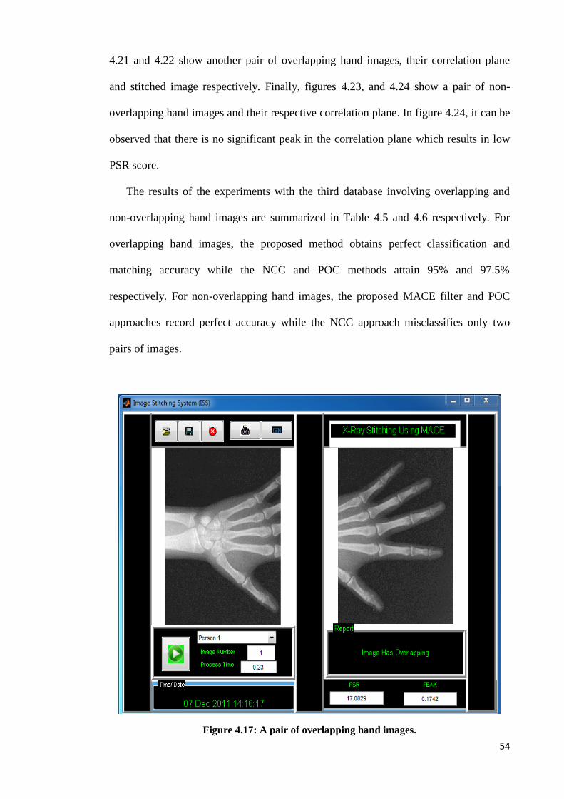
54
4.21 and 4.22 show another pair of overlapping hand images, their correlation plane
and stitched image respectively. Finally, figures 4.23, and 4.24 show a pair of non-
overlapping hand images and their respective correlation plane. In figure 4.24, it can be
observed that there is no significant peak in the correlation plane which results in low
PSR score.
The results of the experiments with the third database involving overlapping and
non-overlapping hand images are summarized in Table 4.5 and 4.6 respectively. For
overlapping hand images, the proposed method obtains perfect classification and
matching accuracy while the NCC and POC methods attain 95% and 97.5%
respectively. For non-overlapping hand images, the proposed MACE filter and POC
approaches record perfect accuracy while the NCC approach misclassifies only two
pairs of images.
Figure 4.17: A pair of overlapping hand images.
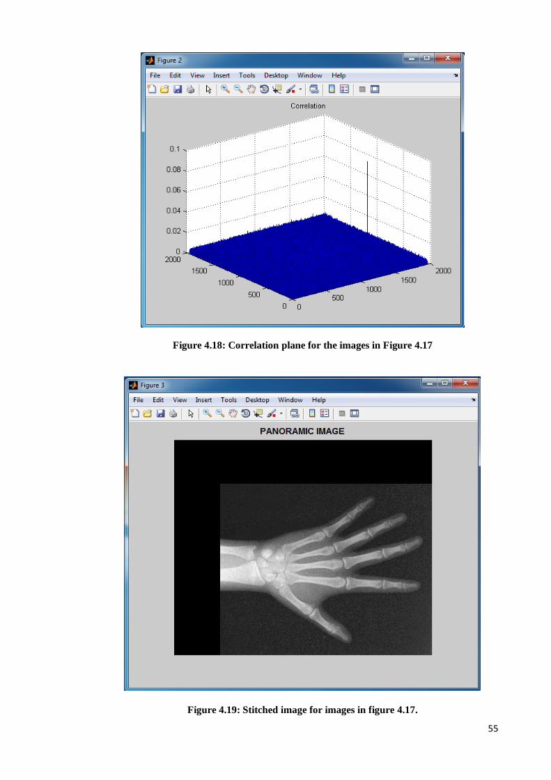
55
Figure 4.18: Correlation plane for the images in Figure 4.17
Figure 4.19: Stitched image for images in figure 4.17.

56
Figure 4.20: Result of Peak and PSR of Two Positive Overlapped Images.
Figure 4.21: Correlation plane for the images in Figure 4.20

57
Figure 4.22: Stitched image for images in figure 4.20.

58
Figure 4.23: Result of Peak and PSR Value for Non-Overlapped Image

59
Figure 4.24: Correlation plane for non-overlapping images
Table 4.5: Evaluation of matching precision of medical Stitching System using (TPR) and
(FNR) Rates
Methods Total number
of overlapped
images in
database
No. of overlapped
images correctly
identified and
stitched (TPR)
TPR (%) FNR (%) Average
processing
time
(second)
Proposed 40 40 100% 0% 0.3
NCC 40 38 95% 5% 1.2
POC 40 39 97.5% 2.5% 0.5

60
Table 4.6: Evaluation of matching precision of stitching system using (TNR) and (TPR)
Rates
Methods Total number
of none
overlapped
images in
database
No. of non
overlapped images
correctly identified
(FPR)
FPR
(%)
TNR (%) Average
processing
time
(second)
Proposed 40 40 100% 0% 0.18
NCC 40 39 97.5% 2.5% 0.88
POC 40 40 100% 0% 0.41
4.6 Summary
The performance of the proposed method based on the MACE correlation filter is
investigated in this chapter. The ability of the method to classify overlapping and non-
overlapping pairs of images is demonstrated using 3 sets of databases. Then the
performance of the proposed method is compared to those of the NCC and POC
approaches. It is observed that the proposed method displays comparable or superior
performance to the other two methods in all instances on the three standard databases.
These results are promising and demonstrate the potential of the proposed method for
further development to tackle more advanced stitching problems that may involve
image warping, rotation and scale variations, slant and tilt.
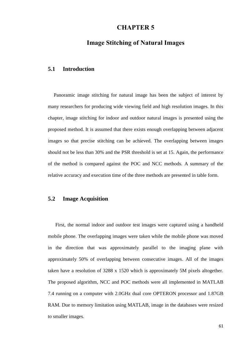
61
CHAPTER 5
Image Stitching of Natural Images
5.1 Introduction
Panoramic image stitching for natural image has been the subject of interest by
many researchers for producing wide viewing field and high resolution images. In this
chapter, image stitching for indoor and outdoor natural images is presented using the
proposed method. It is assumed that there exists enough overlapping between adjacent
images so that precise stitching can be achieved. The overlapping between images
should not be less than 30% and the PSR threshold is set at 15. Again, the performance
of the method is compared against the POC and NCC methods. A summary of the
relative accuracy and execution time of the three methods are presented in table form.
5.2 Image Acquisition
First, the normal indoor and outdoor test images were captured using a handheld
mobile phone. The overlapping images were taken while the mobile phone was moved
in the direction that was approximately parallel to the imaging plane with
approximately 50% of overlapping between consecutive images. All of the images
taken have a resolution of 3288 x 1520 which is approximately 5M pixels altogether.
The proposed algorithm, NCC and POC methods were all implemented in MATLAB
7.4 running on a computer with 2.0GHz dual core OPTERON processor and 1.87GB
RAM. Due to memory limitation using MATLAB, image in the databases were resized
to smaller images.

62
Figure 5.1: image acquisition using mobile phone
5.3 Indoor image stitching
For indoor image stitching, two sets of experiments were carried out using 40 pairs
of overlapping and 40 pairs of non-overlapping indoor images. In the first set of
experiments, the 40 overlapping images were analyzed using the MACE filter
approach. Then the same sets of experiments were carried out using NCC and POC
methods. Figures 5.2, 5.3 and 5.4 show a pair of overlapping indoor images, their
correlation plane and the final stitched image respectively. The average processing
time, peak and PSR values of the three methods for the two images in Figure 5.2 are
presented in Table 5.1.
Translation
distance, t
d
l
L
Image 2 Image 1

63
Figure 5.2: Two overlapping indoor images
Figure 5.3: Correlation plane for images in Figure 5.2
PANORAMA IMAGE

64
Figure 5.4: Stitched image for images in Figure 5.2
Table 5.1: Execution time, peak and PSR values for images in Figure 5.2
Method Execution Time Peak PSR
Proposed 2.14 0.217 17.047
POC 3.68 0.172 16.223
NCC 5.12 0.197 16.344
Similarly, figure 5.5 shows another pair of overlapping images whose final stitched
image is given in figures 5.6. The correlation plane for overlapping image will be same
as in figure 5.3. The average processing time, peak and PSR values of the three
methods for the two referred images are presented in Table 5.2.
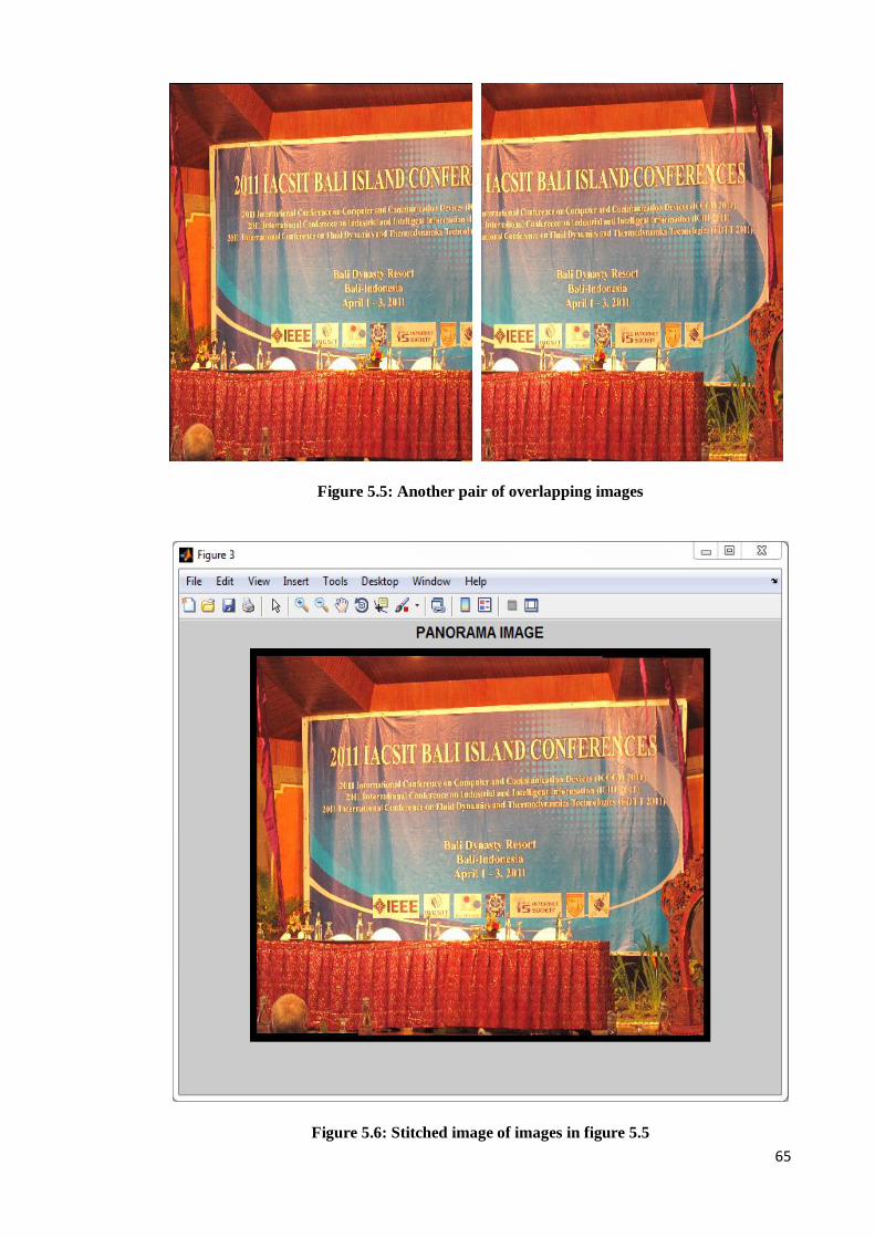
65
Figure 5.5: Another pair of overlapping images
Figure 5.6: Stitched image of images in figure 5.5
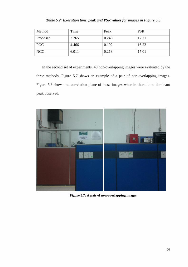
66
Table 5.2: Execution time, peak and PSR values for images in Figure 5.5
Method Time Peak PSR
Proposed 3.265 0.243 17.21
POC 4.466 0.192 16.22
NCC 6.011 0.218 17.01
In the second set of experiments, 40 non-overlapping images were evaluated by the
three methods. Figure 5.7 shows an example of a pair of non-overlapping images.
Figure 5.8 shows the correlation plane of these images wherein there is no dominant
peak observed.
Figure 5.7: A pair of non-overlapping images
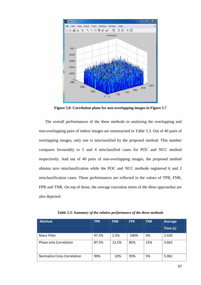
67
Figure 5.8: Correlation plane for non-overlapping images in Figure 5.7
The overall performances of the three methods in analysing the overlapping and
non-overlapping pairs of indoor images are summarized in Table 5.3. Out of 40 pairs of
overlapping images, only one is misclassified by the proposed method. This number
compares favourably to 5 and 4 misclassified cases for POC and NCC method
respectively. And out of 40 pairs of non-overlapping images, the proposed method
obtains zero misclassification while the POC and NCC methods registered 6 and 2
misclassification cases. These performances are reflected in the values of TPR, FNR,
FPR and TNR. On top of those, the average execution times of the three approaches are
also depicted.
Table 5.3: Summary of the relative performance of the three methods
Method
TPR FNR FPR TNR Average
Time (s)
Mace Filter 97.5% 2.5% 100% 0% 2.426
Phase only Correlation 87.5% 12.5% 85% 15% 3.662
Normalize Cross Correlation 90% 10% 95% 5% 5.061

68
5.4 Outdoor image stitching
For outdoor image stitching, 40 sets of overlapping images and 40 sets of non-
overlapping images were analyzed by the three methods. Each set contains 4 images. A
set of images are shown in figure 5.9 the final panorama image is shown in figure 5.10.
The process started with stitching a pair of images followed by merging the other two
images to the stitched image consecutively. For each successive merging a processing
time, peak and PSR were recorded. Then the same procedure was repeated using the
POC and NCC methods. The values of the total execution time, peaks and PSR for the
three methods in stitching the four images are given in Table 5.4.
Another set of images are shown in figure 5.11 and the final panoramic image is
given in figure 5.12. The values of the total execution time, peaks and PSR for these
images are given in Table 5.5.
Figure 5.9: A set of overlapping outdoor images
PANORAMA IMAGEPANORAMA IMAGE
PANORAMA IMAGE PANORAMA IMAGE

69
Figure 5.10: Final panorama image
Table 5.4: Execution times, peaks and PSRs of the three methods in merging 4 outdoor
images successively into a single image in figure5. 9.
Method Total execution
time
Peak PSR
Proposed 5.675 (0.433,0.637,0.523) (17.27,17.22,17.31)
POC 6.863 (0.352,0.572,0.492) (16.53,16.86,16.11)
NCC 8.844 (0.414,0.598,0.511) (17.11,17.03,16.28)
Figure 5.11: sequence of input images

70
Figure 5.12: Panorama in Kashiwazaki, Japan
Table 5.5: Execution times, peaks and PSRs of the MACE, POC and NCC methods in
constructing the panoramic image of figure 5.11.
Method Time Peak PSR
Proposed 6.11 (0.597,0.637,0.524) (17.303,17.286,17.298)
POC 7.21 (0.437,0.544,0.464) (16.931,16.432,16.646)
NCC 9.23 (0.511,0.612,0.518) (17.210,17.153,17.173)
Table 5.6 presents the overall performances of the three methods in analysing both
the overlapping and non-overlapping sets of outdoor images. It should be noted that in
a single set of overlapping images, all images must be classified and stitched correctly
for the set to be included in the TPR. Similarly, in the calculation for FPR, each pair of
consecutive images in a set must be declared as non-overlapping before the set can be
considered as correctly classified. All 40 sets of overlapping outdoor images were
classified and stitched correctly by the proposed method. The POC misclassified 3 sets
of images while the NCC missed 1 set of images. And out of 40 non-overlapping sets
of images, the proposed method and the NCC obtained zero misclassification whiles

71
the POC method 1 misclassification case. These results are represented by the values of
TPR, FNR, FPR and TNR in the table.
Table 5.6: Summary of the relative performance of the three methods
Method
TPR FNR FPR TNR Average
time (s)
Mace Filter 100% 0% 100% 0% 5.81
Phase only
Correlation
92.5% 7.5% 97.5% 2.5% 6.88
Normalize Cross
Correlation
97.5% 2.5% 100% 0% 9.04
5.5 Summary
This chapter describes the experiments that explore the ability of the proposed
approach to classify overlapping and non-overlapping natural images in sets of four.
When sets of overlapping or non-overlapping indoor or outdoor images are presented to
the proposed method as inputs, it calculates the measure of correlation between
consecutive images and determines whether they are overlapping or not. If the images
are deemed to be overlapping they will be stitched to form a single image. Then the
same experiments are repeated using POC and NCC methods. The results show the
superiority of the proposed method against the POC and NCC methods in terms of
classification accuracy and execution time.
72
CHAPTER 6
Conclusion
6.1 Introduction
The objective of the thesis is to developed a panorama stitching using Minimum
Average Correlation Energy (MACE) filter. The ability of the method to classify non-
overlapping and overlapping images is tested on pairs of radiographic images and sets
of natural indoor and outdoor images. If the images are classified as overlapping, they
are then stitched accordingly. The performance of the method is compared to those of
the Phase Only Correlation (POC) and Normalized Cross Correlation (NCC) in terms
of accuracy and computation time.
6.2 Summary of Work
Given pairs or sets of images, the implementation of the proposed method starts
with pre-processing and followed by Fourier transformation, MACE filter design,
inverse transformation, peak and Peak to Sidelobe Ratio (PSR) measurement and image
blending. The accuracy of the method is then measured in terms of TPR, FPR, TNR
and FNR. On the other hand, its efficiency is measured by the average processing or
execution time. Its relative performance is compared against two other correlation
based methods, specifically, the NCC and POC methods.
Both overlapping and non-overlapping sets of images are presented to the three
methods to test their classification and stitching ability. Various pairs of radiographic
images and sets of natural images are utilized in the experiments. It turns out that the

73
performance of the proposed method is comparable or better than those of the POC and
NCC methods while its execution time is always less than those recorded by the other
two methods. In short, under the constraints of at least 30% overlapping and minimal
rotation, skew, tilt and scaling, the proposed method performs satisfactorily.
6.3 Future Work
Despite the encouraging results, there are always avenues to enhance the
performance and robustness of the method. Since the setting of medical images is
usually restrictive, variations in the forms of rotation, scaling and affine translation are
usually minimal. In this regard, it is suggested for future work that processing is
performed both in the time and frequency domains so that the amount of 30%
overlapping that is necessary for correct stitching can be reduced. For natural image
stitching, further study can be done on improving the model of the process to overcome
effects of image warping, rotation, scaling, slant, tilt and affine translation.
6.4 Summary
The following points are summarized from the thesis
· A new stitching method based on MACE filter is proposed
· The utility of the method is tested on radiographic and natural images
· Its performance is compared to two similar methods

74
References
. Application note, understanding FFT window. from www.Ids-group.com Asher, M. A., & Burton, D. C. (2006). Adolescent idiopathic scoliosis: natural history and long
term treatment effects. Scoliosis, 1(1), 2. Awcock, G. J., & Thomas, R. (1995). Applied image processing: McGraw-Hill, Inc. Bettinardi, V., Gilardi, M.C., Lucignani, G., Landoni, C., & Rizzo, G. (1993). A procedure for
patient repositioning and compensation for misalignment between transmission and emission data in PET heart studies. J. Nucl. Med., 34(1), 137-142.
Bidaut, L. M., & Vallee, J.P. (2001). Automated registration of dynamic MR images for the quantification of myocardial perfusion. J. Magn. Res. Imag, 13, 648-655.
Brown, L. G. (1992). A survey of image registration techniques. ACM Computing Surveys, 24, 326-376.
Brown, M., & Lowe, D.G. (2007). Automatic Panoramic Image Stitching Uisng Invariant Features. International Journal of Computer Vision 74(1), 59-73.
Brown, M., & Lowe, D. G. (2003). Recognising panoramas. Čapek, M., Wegenkittl, R., & Felkel, P. . (2002). A Fully Automatic Stitching of 2D Medical Data
Sets. BIOSIGNAL, 16, 326-328. Chen, C. Y. (1998). Image Stitching - Comparisons and New Techniques. CITR-TR-30. da Fontoura Costa, L., & Cesar, R. M. (2009). Shape classification and analysis: theory and
practice (Vol. 10): CRC. Feng, Z., Qingming, H., Hao, W., & Wen, G. (2010). MOCC: A Fast and Robust Correlation-
Based Method for Interest Point Matching under Large Scale Changes. . EURASIP Journal on Advances in Signal Processing, 16.
Fitzpatrick, J. M., Hill, D. L. G., & Maurer, C.R. (2000). Image Registration Handbook of Medical Imaging (pp. 375-435). Bellingham: WA: SPIE Press.
Gonzalez, R. C., Woods, R., & Eddins, S. L. Digital image processing using MATLAB. 2004. Publishing House of Electronics Industry.
Harris, C. (1993). Geometry from visual motion. Harris, C., & Stephens, M. (1988). A combined corner and edge detector. Hoh, C. K., Dahlbom, M., Harris, G., Choi, Y., Hawkins, R. A., Phelps, M.E., Maddahi, J. (1993).
Automated iterative three-dimensional registration of positron emission tomography images. nuclear medicine official publication Society of Nuclear Medicine, 34(2), 2009-2018.
Ito, K., Aoki, T., Nakajima, H., Kobayashi, K., & Higuchi, T. (2006). A palmprint recognition algorithm using phase-based image matching.
Kumar, A., Bandaru, R. S.,Rao, B. M., Kulkarni, S., Ghatpande, N. . (2010). Automatic Image Alignment and Stitching ofMedical Images with Seam Blending. World Academy of Science, Engineering and Technology, 65.
Lagendijk, R. L., & Biemond, J. (1999). Basic methods for image restoration and identification. Handbook of Image and Video Processing, A. Bovik, ed.(Academic, 2000).
Lee, J., Lee, W., Cho, I., & Jeong, D. (2005). Fast Panoramic Image Generation Method Using Morphological Corner Detection. PCM, 547-558.
Lepetit, V., & Fua, P. (2004). Towards recognizing feature points using classification trees. Lausanne: EPFL Technical Report IC/2004/74.
Lepetit, V., & Fua, P. (2006). Keypoint recognition using randomized trees. Pattern Analysis and Machine Intelligence, IEEE Transactions on, 28(9), 1465-1479.
Lewis, J. (1995). Fast normalized cross-correlation.

75
Li, Y., & Ma, L. (2006). A fast and robust image stitching algorithm. Paper presented at the Intelligent Control and Automation, 2006. WCICA 2006. The Sixth World Congress on Dailan.
Lowe, D. G. (1999). Object recognition from local scale-invariant features. Lowe, D. G. (2004). Distinctive Image Features from Scale-Invariant Keypoints. International
Journal of Computer Vision Maintz, J., & Viergever, M. A. (1998). A survey of medical image registration. Medical image
analysis, 2(1), 1-36. Makela, T., Clarysse, P., Sipila, O., Pauna, N., Pham, Q. C., Katila, T., & Magnin, I. E. (2002). A
review of cardiac image registration methods. Medical Imaging, IEEE Transactions on, 21(9), 1011-1021.
Matsumoto, T., Takahashi, T., Iwahashi, M., Kimura, T., Salbiah, S. & Mokhtar, N. (2010). Reduction of data size for transmission in localization of mobile robots. International Journal of the Physical Sciences, 5(17), 2652-2657.
Matsumoto, T., Takahashi, T., Iwahashi, M., Kimura, T., Salbiah, S. & Mokhtar, N. (2011). Visual compensation in localization of a robot on a ceiling map. Scientific Research and Essays, 6(1), 131-135.
Milgram, D. L. (1975). Computer methods for creating photomosaics. Computers, IEEE Transactions on, 100(11), 1113-1119.
Moravec, H. P. (1981). Rover visual obstacle avoidance. O’Connor, M. K. (2000). Evaluation of motion-correction techniques in cardiac SPECT. J. Nucl.
Med., 41(7). O’Connor, M. K., Kanal, K. M., Gebhard, M. W., & Rossman, P. J. . (1998). Comparison of four
motion correction techniques in SPECT imaging of the heart: A cardiac phantom study. J. Nucl. Med., 39, 2027-2034.
Paul, V. W. M. W. I. (1997). Alignment by Maximization of Mutual Information. International Journal of Computer Vision, 24(2), 137–154.
Rankov, V., Locke, R. J., Edens, R. J., Barber, P. R., & Vojnovic, B. (2005). An algorithm for image stitching and blending.
Savvides, M., Kumar, B. V. K. V., & Khosla, P. (2002). Face verification using correlation filters. 3rd IEEE Automatic Identification Advanced Technologies, 56-61.
Schmid, C., & Mohr, R. (1997). Local grayvalue invariants for image retrieval. Pattern Analysis and Machine Intelligence, IEEE Transactions on, 19(5), 530-535.
Slomka, P. J., Gilbert, A. H., Stephenson, J., & Cradduck, T. (1995). Automated Alignment and Sizing of Myocardial Stress and Rest Scans to Three-Dimensional Normal Templates Using an Image Registration Algorithm. The Journal of Nuclear Medicine, 36, 1115-1122.
slomka, P. J., Radau, P., Hurwitz, G. A.,Dey, D. (2001). Automated three dimensional quantification of myocardial perfusion and brain SPECT. Comput. Med. Imag. Graph(no.25), 153-164.
Steedly, D., Pal, Chris., & Szeliski, R. . (2005). Efficiently Registering Video into Panoramic Mosaics. Paper presented at the International Conference on Computer Vision.
Szeliski, R. (2006). Image alignment and stitching: a tutorial. Found. Trends. Comput. Graph. Vis., 2(1), 1-104. doi: 10.1561/0600000009
Takita, K., Aoki, T., Sasaki, Y., Higuchi, T., & Kobayashi, K. (2003). High-accuracy subpixel image registration based on phase-only correlation. IEICE TRANSACTIONS ON FUNDAMENTALS OF ELECTRONICS COMMUNICATIONS AND COMPUTER SCIENCES E SERIES A, 86(8), 1925-1934.
Torr, P. H. S. (1995). Motion segmentation and outlier detection. University of Oxford. Turkington, T. G., DeGrado,T.R., Hanson,M.W., & Coleman, R. E. (1997). Alignment of dynamic
cardiac PET images for correction of motion. IEEE Trans. Nucl. Sci., 44, 235-242.

76
W.C. Hu, C. H. C., Y.F. Liang, and C.T. Wu. (2007). An effective blending method for panoramic images in imagebased virtual reality. Paper presented at the International Conference on Advanced Information Technologies, Taichung, Taiwan.
Wang, Q., & You, S. (2008). Feature selection for real-time image matching systems. Wang, Y., & Wang, M. . (2010). Research on Stitching Technique of Medical Infrared Images.
Paper presented at the International Conference on Computer Application and System Modeling Taiyuan.
Xiao, D., & Ohya, J. (2007). Contrast enhancement of color images based on wavelet transform and human visual system.
Xiong, Y., & Pulli, K. (2010). Fast panorama stitching for high-quality panoramic images on mobile phones. Consumer Electronics, IEEE Transactions on, 56(2), 298-306.
Zhang, Z., Deriche, R., Faugeras, O., & Luong, Q. T. (1995). A robust technique for matching two uncalibrated images through the recovery of the unknown epipolar geometry. Artificial intelligence, 78(1-2), 87-119.
Zheng, J. Y., & Tsuji, S. (1992). Panoramic Representation for Route Recognition by a Mobile Robot. International Journal of Computer Vision 9, 55-76.
Zitova, B., & Flusser, J. (2003). Image registration methods: a survey. Image and Vision Computing, 21(11), 977-1000.


