-- --

Image Segmentation

• Goals and Difficulties

- The goal of segmentation is to partition an image into regions (e.g.,separate objects from background)

- The results of segmentation are very important in determining theev entual success or failure of image analysis

- Segmentation is very a very difficult problem in general !!

• Increasing Accuracy and Robustness

- Introduce enough knowledge about the application domain

- Control the environment (e.g., in industrial applications)

- Select type of sensors to enhance the objects of interest

(e.g, use infrared imaging for target recognition applications)

-- --

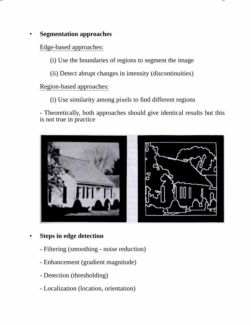
• Segmentation approaches

Edge-based approaches:

(i) Use the boundaries of regions to segment the image

(ii) Detect abrupt changes in intensity (discontinuities)

Region-based approaches:

(i) Use similarity among pixels to find different regions

- Theoretically, both approaches should give identical results but thisis not true in practice

• Steps in edge detection

- Filtering (smoothing - noise reduction)

- Enhancement (gradient magnitude)

- Detection (thresholding)

- Localization (location, orientation)

-- --

Detecting Discontinuities

• General Idea

- Apply a mask over the image

- Apply thresholding: If |R| > T, then discontinuity !!

input image

w1 w2 w3

w4 w5 w6

w7 w8 w9

z1 z2 z3

z4 z5 z6

z7 z8 z9

z5’

z5’ = R = w1z1 + w2z2 + ... + z9w9

convolved image

• Point Detection

8

-1 -1

-1 -1

-1 -1 -1

-1

1

10

1 1 1 1

1 1 1 1

1 1 1 1

1 1 1 1 1

1 1 1 1 1

1

- - - - -

-

-

-

-----

-

-

- 72 -9 0

-9 -9 0

0 0 0

* =

original image convolved image

mask

- Depending on the value of T , we get 4 points (0 < T ≤ 9), 1 point(9 < T ≤ 72) or 0 points (T > 72)

-- --

• Line detection

- The masks shown below can be used to detect lines at various orien-tations

-1 -1

-1 -1 -1

-1

*

mask

2 2 2

=

=

0 0 0 0

0000

1 1 1 1

1

1

1

0

0

0

0

0

0

0

0

0

- - - -

-

----

-

- - - -

-

----

-

6 6

0 0

horizontal line

vertical line

convolved image

convolved image

-- --

- In practice, we run every mask over the image and we combine theresponses:

R(x, y) = max(|R1(x, y)|, |R2(x, y)|, |R3(x, y)|, |R4(x, y)|)

If R(x, y) > T , then discontinuity

-1 -1

-1 -1 -1

-1 -1-1 -1

-1 -1

-1

2

-1 -1

-1 -1

2

-1 -1 -1222 2 -1

-1-12

2

-1

2

2

2

2

-1

Original Image

R1 R2 R3 R4

Convolved Image with R1

Convolved Image with R2

Convolved Image Convolved Image with R4 with R3

. . .

.

.

(x,y)

(x,y) (x,y) (x,y) (x,y)

MAX

-- --

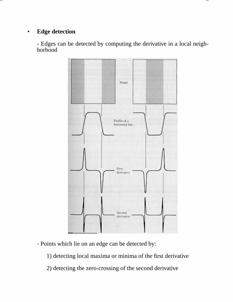
• Edge detection

- Edges can be detected by computing the derivative in a local neigh-borhood

- Points which lie on an edge can be detected by:

1) detecting local maxima or minima of the first derivative

2) detecting the zero-crossing of the second derivative

-- --

• Computing edges using the first derivative

- Compute the gradient !!

∇ f =

∂ f

∂x∂ f

∂y

magnitude(∇ f ) = √ (∂ f

∂x)2 + (

∂ f

∂y)2 = √ Gx

2 + Gy2

(can be approximated by: |Gx | + |Gy |)

direction(∇ f ) = tan−1(Gy/Gx)

- Steps

1) Gx = f (x, y) * Mx(x, y)

2) Gy = f (x, y) * My(x, y)

3) M(x, y) = |Gx | + |Gy |

4) a(x, y) = tan−1(Gy/Gx)

5) If M(x, y) > T , then discontinuity

-- --

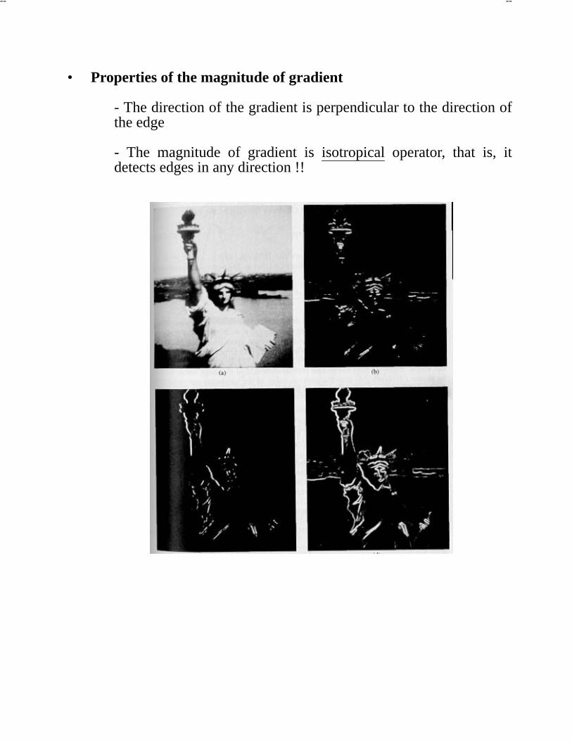
• Properties of the magnitude of gradient

- The direction of the gradient is perpendicular to the direction ofthe edge

- The magnitude of gradient is isotropical operator, that is, itdetects edges in any direction !!

-- --

• Computing edges using the second derivative

- The second derivative can be obtained using the Laplacian

∇2 f =∂2 f

∂2 x+

∂2 f

∂2 y

- Approximating ∇2 f

∂2 f

∂2 x= f (x − 1, y) − 2 f (x, y) + f (x + 1, y)

∂2 f

∂2 y= f (x, y − 1) − 2 f (x, y) + f (x, y + 1)

∇2 f = − 4 f (x, y) + f (x + 1, y) + f (x − 1, y) + f (x, y + 1) + f (x, y − 1)

Z1 Z2 Z3

Z4 Z5 Z6

Z7 Z8 Z9 ∇2 f = − 4z5 + (z2 + z4 + z6 + z8)

- The Laplacian can be implemented using the mask shown below

0 0

1 1

0 1 0

-4

1

-- --

• Properties of the second derivative

- It is an isotropic operator

- It is cheaper to implement (one mask only)

- It does not provide information about edge direction

- It is more sensitive to noise (differentiates twice)

- To reduce the noise effect, the image should be first smoothed with alow-pass filter

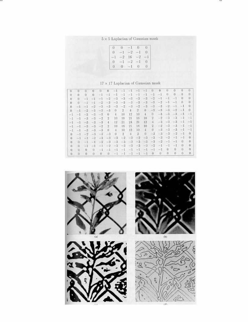
• The Laplacian-of-Gaussian (LOG) edge detector

- The low-pass filter is chosen to be a Gaussian

h(x, y) = e−

x2+y2

2σ 2

(σ determines the degree of smoothing, mask size increases with σ )

- It can be shown that

∇2[ f (x, y) * h(x, y)] = ∇2h(x, y) * f (x, y)

∇2h(x, y) = (r2 − σ 2

σ 4)e−r2/2σ 2

, (r2 = x2 + y2)

-- --

-- --

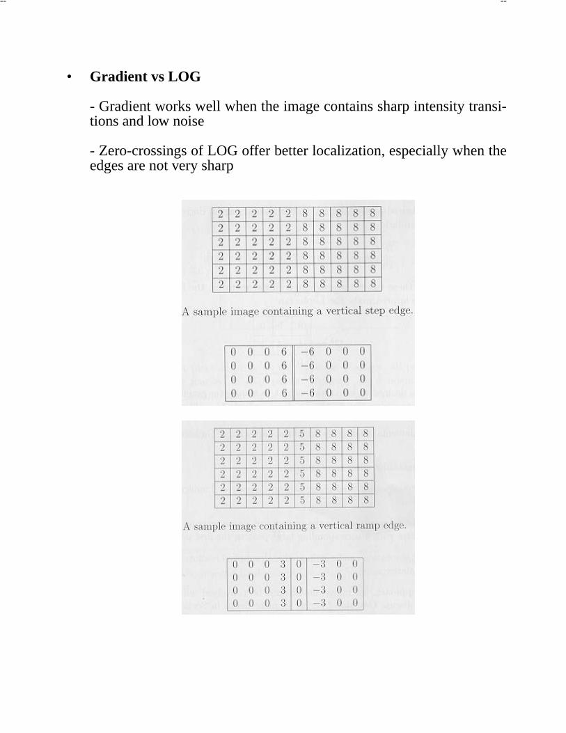
• Gradient vs LOG

- Gradient works well when the image contains sharp intensity transi-tions and low noise

- Zero-crossings of LOG offer better localization, especially when theedges are not very sharp

-- --

Edge Linking and Boundary Detection

- Edge detection does not yield connected boundaries

- Edge linking and boundary following must be applied after edgedetection

• Local processing methods

- At each pixel, a neighborhood (e.g., 3x3) is examined

- Pixels which are similar in this neighborhood are linked

- How do we define similarity ?

|∇ f (x, y) − ∇ f (x′, y′)| ≤ T (magnitude)

|a(x, y) − a(x′, y′)| ≤ A (direction)

-- --

• Global processing methods

- If the gaps between pixels are very large, local processing methodsare not effective

- Model-based approaches can be used in this case !!

- Hough Transform can be used to determine whether points lie on acurved of a specified shape

Using Hough Transform to detect lines

- Consider the slope-intercept equation of line

y = ax + b,

(a, b are constants, x is a variable, y is a function of x)

- Rewrite the equation as follows:

b = −xa + y

(now, x, y are constants, a is a variable, b is a function of a)

-- --

- The following properties are true:

Each point (xi, yi) defines a line in the a − b space (parameterspace)

Points lying on the same line in the x − y space, define lines in theparameter space which all intersect at the same point

The coordinates of the point of intersection define the parametersof the line in the x − y space

• Algorithm

1. Quantize the parameter spaceP[amin, . . . , amax][bmin, . . . , bmax] (accumulator array)

2. For each edge point (x, y)

For(a = amin; a ≤ amax; a++) {

b = − xa + y; /* round off if needed *

(P[a][b])++; /* voting */

}

3. Find local maxima in P[a][b]

(If P[a j][bk]=M, then M points lie on the line y = a j x + bk)