![Advances in Phytoplankton Pigment Mapping in Spanish ... · Advances in Phytoplankton Pigment Mapping in Spanish Reservoirs ... Vol Cla] Clorofila a (mg/m 3) Alcántara ... Advances](https://static.fdocuments.in/doc/165x107/5bb20be209d3f2272e8c2061/advances-in-phytoplankton-pigment-mapping-in-spanish-advances-in-phytoplankton.jpg)
Image Segmentation and Pigment Mapping of Cultural ... · Image Segmentation and Pigment Mapping of...
346
Image Segmentation and Pigment Mapping of Cultural Heritage Based on Spectral Imaging by Yonghui Zhao A dissertation proposal submitted in partial fulfillment of the requirements for the degree of Doctor of Philosophy in the Chester F. Carlson Center for Imaging Science Rochester Institute of Technology March 10, 2008
Transcript of Image Segmentation and Pigment Mapping of Cultural ... · Image Segmentation and Pigment Mapping of...

Image Segmentation and Pigment Mapping of Cultural Heritage Basedon Spectral Imaging
by
Yonghui Zhao
A dissertation proposal submitted in partial fulfillment of the
requirements for the degree of Doctor of Philosophy
in the Chester F. Carlson Center for Imaging Science
Rochester Institute of Technology
March 10, 2008

CHESTER F. CARLSON CENTER FOR IMAGING SCIENCE
ROCHESTER INSTITUTE OF TECHNOLOGY
ROCHESTER, NEW YORK
CERTIFICATE OF APPROVAL
Ph.D. DEGREE DISSERTATION
The Ph.D. Degree Dissertation of Yonghui Zhaohas been examined and approved by the
dissertation committee as satisfactory for thedissertation required for the
Ph.D. degree in Imaging Science
Dr. Roy S. Berns, dissertation Advisor
Dr. Joseph G. Voelkel
Dr. David W. Messinger
Dr. Mark D. Fairchild
Date

DISSERTATION RELEASE PERMISSION
ROCHESTER INSTITUTE OF TECHNOLOGY
CHESTER F. CARLSON CENTER FOR IMAGING SCIENCE
Title of Dissertation:
Image Segmentation and Pigment Mapping of Cultural Heritage Based on
Spectral Imaging
I, Yonghui Zhao, hereby grant permission to Wallace Memorial Library of R.I.T. to
reproduce my thesis in whole or in part. Any reproduction will not be for commercial
use or profit.
SignatureDate

Image Segmentation and Pigment Mapping of Cultural Heritage Basedon Spectral Imaging
by
Yonghui Zhao
Submitted to theChester F. Carlson Center for Imaging Science
in partial fulfillment of the requirementsfor the Doctor of Philosophy Degree
at the Rochester Institute of Technology
Abstract
The goal of the work reported in this dissertation is to develop methods for im-
age segmentation and pigment mapping of paintings based on spectral imaging. To
reach this goal it is necessary to achieve sufficient spectral and colorimetric accuracies
of both the spectral imaging system and pigment mapping. The output is a series of
spatial distributions of pigments (or pigment maps) composing a painting. With these
pigment maps, the change of the color appearance of the painting can be simulated
when the optical properties of one or more pigments are altered. These pigment maps
will also be beneficial for enriching the historical knowledge of the painting and aid-
ing conservators in determining the best course for retouching damaged areas of the
painting when metamerism is a factor.
First, a new spectral reconstruction algorithm was developed based on Wyszecki’s
hypothesis and the matrix R theory developed by Cohen and Kappauf. The method
achieved both high spectral and colorimetric accuracies for a certain combination of
illuminant and observer. The method was successfully tested with a practical spectral
imaging system that included a traditional color-filter-array camera coupled with two

5
optimized filters, developed in the Munsell Color Science Laboratory. The spectral
imaging system was used to image test paintings, and the method was used to retrieve
spectral reflectance factors for these paintings.
Next, pigment mapping methods were brought forth, and these methods were based
on Kubelka-Munk (K-M) turbid media theory that can predict spectral reflectance fac-
tor for a specimen from the optical properties of the specimen’s constituent pigments.
The K-M theory has achieved practical success for opaque materials by reduction in
mathematical complexity and elimination of controlling thickness. The use of the gen-
eral K-M theory for the translucent samples was extensively studied, including deter-
mination of optical properties of pigments as functions of film thickness, and prediction
of spectral reflectance factor of a specimen by selecting the right pigment combination.
After that, an investigation was carried out to evaluate the impact of opacity and layer
configuration of a specimen on pigment mapping. The conclusions were drawn from
the comparisons of prediction accuracies of pigment mapping between opaque and
translucent assumption, and between single and bi-layer assumptions.
Finally, spectral imaging and pigment mapping were applied to three paintings.
Large images were first partitioned into several small images, and each small image
was segmented into different clusters based on either an unsupervised or supervised
classification method. For each cluster, pigment mapping was done pixel-wise with a
limited number of pigments, or with a limited number of pixels and then extended to
other pixels based on a similarity calculation. For the masterpiece The Starry Night,
these pigment maps can provide historical knowledge about the painting, aid conser-
vators for inpainting damaged areas, and digitally rejuvenate the original color appear-
ance of the painting (e.g. when the lead white was not noticeably darkened).

Acknowledgements
I would like to first thank my advisor, Dr. Roy S. Berns, for his patience, inspiring ad-
vices and ceaseless efforts in teaching me how to become a research scientist. Without
his supervision, this research work would not have been a reality. He has also been a
wonderful role model and a great mentor for me.
I would like to thank Dr. Joseph G. Voelkel, Dr. David W. Messinger and Dr. Mark
D. Fairchild for serving on my thesis committee and reviewing my thesis. I highly
appreciate their help and consideration for arranging my candidacy exam and final
defense. Thanks again for your valuable time and guidance.
I would like to thank Lawrence A. Taplin for his help on operating the spectral
camera, writing efficient programs, and inspiring discussion - Thank you Lawrence.
I would also like to extend my gratitude to all the people of the Munsell Color
Science Laboratory for the help given during the various stages of my thesis, especially
Dr. Mitchell R. Rosen, Dr. David R. Wyble, Dr. Philipp Urban, Mr. Rodney L.
Heckaman, Dr. Yongda Chen, Mahdi Nezamabadi, Mahnaz Mohammadi, Dr. Hongqin
Zhang, Changmeng Liu, Dr. Jiaotao kuang, Valerie Hemink and Colleen M. Desimone.
I would also like to thank the artist, Bernard Lehmann, who had drawn two won-
derful paintings for my research. Both paintings are very good targets for both imaging
and reproduction.
I would also like to thank the Andrew W. Mellon Foundation, the National Gallery
of Art, Washington, the Museum of Modern Art, New York, the Institute of Museum
and Library Services, and Rochester Institute of Technology for their financial support.
Finally, I would like to thank a very special person, my dear husband, for his help
on the proofreading of this dissertation. Thank you for supporting me all the time and
giving me a shoulder to lean on when times were hard.

This work is dedicated to my parents, my husband, Ligang and my lovely son, Eric for
their love and support.

Contents
1 Introduction 34
1.1 Motivation . . . . . . . . . . . . . . . . . . . . . . . . . . . . . . . . 34
1.2 Dissertation Outline . . . . . . . . . . . . . . . . . . . . . . . . . . . 37
1.3 Terminology . . . . . . . . . . . . . . . . . . . . . . . . . . . . . . . 39
2 Background Literature Review 41
2.1 Multispectral Imaging . . . . . . . . . . . . . . . . . . . . . . . . . . 41
2.1.1 Historical Development . . . . . . . . . . . . . . . . . . . . 41
2.1.2 Camera Model . . . . . . . . . . . . . . . . . . . . . . . . . 43
2.1.3 Spectral Reconstruction Algorithms . . . . . . . . . . . . . . 45
2.1.3.1 Direct Reconstruction . . . . . . . . . . . . . . . . 45
2.1.3.2 Reconstruction by Interpolation . . . . . . . . . . . 48
2.1.3.3 Learning-based Reconstruction . . . . . . . . . . . 50
2.1.4 Summary . . . . . . . . . . . . . . . . . . . . . . . . . . . . 53
2.2 Color-Match Prediction for Pigment Materials . . . . . . . . . . . . . 54
2.2.1 Introduction . . . . . . . . . . . . . . . . . . . . . . . . . . . 54
2.2.2 Surface Correction . . . . . . . . . . . . . . . . . . . . . . . 55
2.2.3 Kubelka-Munk Theory . . . . . . . . . . . . . . . . . . . . . 58

CONTENTS 9
2.2.3.1 Historical View . . . . . . . . . . . . . . . . . . . 58
2.2.3.2 General Theory . . . . . . . . . . . . . . . . . . . 59
2.2.3.3 Limitations of Kubelka-Munk Theory . . . . . . . 61
2.2.4 Pigment Mixing Models . . . . . . . . . . . . . . . . . . . . 62
2.2.4.1 Introduction . . . . . . . . . . . . . . . . . . . . . 62
2.2.4.2 Two-Constant Kubelka-Munk Theory . . . . . . . . 63
2.2.4.3 Single-Constant Kubelka-Munk Theory . . . . . . 63
2.2.4.4 Determination of Absorption and Scattering Coeffi-
cients . . . . . . . . . . . . . . . . . . . . . . . . . 64
2.2.5 Summary . . . . . . . . . . . . . . . . . . . . . . . . . . . . 66
2.3 Pigment Identification . . . . . . . . . . . . . . . . . . . . . . . . . . 67
2.3.1 Introduction . . . . . . . . . . . . . . . . . . . . . . . . . . . 67
2.3.2 Modern Analytic Techniques . . . . . . . . . . . . . . . . . . 68
2.3.3 Near Infrared Imaging Spectroscopy . . . . . . . . . . . . . . 69
2.3.4 Visible Reflectance Spectroscopy . . . . . . . . . . . . . . . 73
2.3.5 Summary . . . . . . . . . . . . . . . . . . . . . . . . . . . . 79
2.4 Pigment Mapping . . . . . . . . . . . . . . . . . . . . . . . . . . . . 80
2.4.1 Introduction . . . . . . . . . . . . . . . . . . . . . . . . . . . 80
2.4.2 Pigment Mapping Algorithms . . . . . . . . . . . . . . . . . 81
2.4.3 Summary . . . . . . . . . . . . . . . . . . . . . . . . . . . . 86
3 Image-Based Spectral Reflectance Reconstruction 88
3.1 Introduction . . . . . . . . . . . . . . . . . . . . . . . . . . . . . . . 88
3.2 Matrix R Theory . . . . . . . . . . . . . . . . . . . . . . . . . . . . 89
3.2.1 General Theory . . . . . . . . . . . . . . . . . . . . . . . . . 89
3.2.2 Some Applications . . . . . . . . . . . . . . . . . . . . . . . 91

CONTENTS 10
3.3 Matrix R Method . . . . . . . . . . . . . . . . . . . . . . . . . . . . 94
3.3.1 Spectral Transformation . . . . . . . . . . . . . . . . . . . . 94
3.3.2 Colorimetric Transformation . . . . . . . . . . . . . . . . . . 95
3.3.3 Combination of Two Transformations . . . . . . . . . . . . . 96
3.4 Experimental . . . . . . . . . . . . . . . . . . . . . . . . . . . . . . 97
3.5 Results and Discussions . . . . . . . . . . . . . . . . . . . . . . . . . 99
3.6 Conclusions . . . . . . . . . . . . . . . . . . . . . . . . . . . . . . . 107
4 Pigment Mapping for Opaque Materials 110
4.1 Introduction . . . . . . . . . . . . . . . . . . . . . . . . . . . . . . . 110
4.2 Database Development . . . . . . . . . . . . . . . . . . . . . . . . . 112
4.2.1 Methods . . . . . . . . . . . . . . . . . . . . . . . . . . . . 112
4.2.1.1 Characterization of White Paint . . . . . . . . . . . 113
4.2.1.2 Characterization of Other Paints . . . . . . . . . . . 114
4.2.1.3 Further Simplification . . . . . . . . . . . . . . . . 115
4.2.2 Experimental . . . . . . . . . . . . . . . . . . . . . . . . . . 118
4.2.3 Results and Discussions . . . . . . . . . . . . . . . . . . . . 119
4.2.4 Summary . . . . . . . . . . . . . . . . . . . . . . . . . . . . 120
4.3 Colorant Formulation for Simple Patches . . . . . . . . . . . . . . . 122
4.3.1 Pigment Database . . . . . . . . . . . . . . . . . . . . . . . . 122
4.3.2 Color-Matching Prediction . . . . . . . . . . . . . . . . . . . 123
4.3.3 Summary . . . . . . . . . . . . . . . . . . . . . . . . . . . . 126
4.4 Pigment Mapping for a Complex Image . . . . . . . . . . . . . . . . 128
4.4.1 Introduction . . . . . . . . . . . . . . . . . . . . . . . . . . . 128
4.4.2 Experimental . . . . . . . . . . . . . . . . . . . . . . . . . . 129
4.4.3 Pigment Database . . . . . . . . . . . . . . . . . . . . . . . . 129
CONTENTS 11
4.4.4 Image Segmentation . . . . . . . . . . . . . . . . . . . . . . 130
4.4.5 Pigment Mapping . . . . . . . . . . . . . . . . . . . . . . . . 132
4.4.6 Summary . . . . . . . . . . . . . . . . . . . . . . . . . . . . 135
4.5 Conclusions . . . . . . . . . . . . . . . . . . . . . . . . . . . . . . . 136
5 Improvement of Spectral Imaging by Pigment Mapping 138
5.1 Introduction . . . . . . . . . . . . . . . . . . . . . . . . . . . . . . . 138
5.2 Improved Matrix R Method . . . . . . . . . . . . . . . . . . . . . . . 142
5.3 Experimental . . . . . . . . . . . . . . . . . . . . . . . . . . . . . . 144
5.4 Results and Discussions . . . . . . . . . . . . . . . . . . . . . . . . . 145
5.4.1 Original Matrix R Method . . . . . . . . . . . . . . . . . . . 145
5.4.2 Improved Matrix R Method . . . . . . . . . . . . . . . . . . 147
5.5 Conclusions . . . . . . . . . . . . . . . . . . . . . . . . . . . . . . . 148
6 Color-Match Prediction for Translucent Paints 149
6.1 Introduction . . . . . . . . . . . . . . . . . . . . . . . . . . . . . . . 149
6.2 Database Development . . . . . . . . . . . . . . . . . . . . . . . . . 152
6.2.1 Methods for Determining Optical Constants . . . . . . . . . . 152
6.2.1.1 Black-White Method . . . . . . . . . . . . . . . . 154
6.2.1.2 Infinite Method . . . . . . . . . . . . . . . . . . . 156
6.2.1.3 Masstone-Tint Method . . . . . . . . . . . . . . . 158
6.2.1.4 Two-Region Method . . . . . . . . . . . . . . . . . 160
6.2.2 Problems with Numerical Solutions . . . . . . . . . . . . . . 165
6.2.3 Determination of Optical Constants for White Paints . . . . . 168
6.2.4 Determination of Optical Constants for Other Paints . . . . . 171
6.3 Color-Match Prediction . . . . . . . . . . . . . . . . . . . . . . . . . 174

CONTENTS 12
6.3.1 Opaque vs. Translucent Assumption . . . . . . . . . . . . . . 174
6.3.2 White vs. Black Background . . . . . . . . . . . . . . . . . . 180
6.3.3 Two Worst Examples . . . . . . . . . . . . . . . . . . . . . . 181
6.4 Conclusions . . . . . . . . . . . . . . . . . . . . . . . . . . . . . . . 185
7 Further Investigation of Pigment Mapping 188
7.1 Introduction . . . . . . . . . . . . . . . . . . . . . . . . . . . . . . . 188
7.2 Experimental Setup . . . . . . . . . . . . . . . . . . . . . . . . . . . 190
7.3 Opaque vs. Translucent . . . . . . . . . . . . . . . . . . . . . . . . . 192
7.3.1 Prior Knowledge of Constituent Pigments . . . . . . . . . . . 194
7.3.1.1 Single-Layer Samples Over the White Background . 195
7.3.1.2 Single-Layer Samples Over the Black Background . 199
7.3.1.3 Summary . . . . . . . . . . . . . . . . . . . . . . . 204
7.3.2 Spectrophotometric Measurement . . . . . . . . . . . . . . . 204
7.3.2.1 Single-Layer Samples Over the White Background . 205
7.3.2.2 Single-Layer Samples Over the Black Background . 209
7.3.3 Spectra-based Camera . . . . . . . . . . . . . . . . . . . . . 212
7.4 Single-Layer vs. Bi-Layer . . . . . . . . . . . . . . . . . . . . . . . 217
7.4.1 Prior Knowledge of Constituent Pigments . . . . . . . . . . . 217
7.4.2 Spectrophotometric Measurement . . . . . . . . . . . . . . . 221
7.4.3 Spectral-based Camera . . . . . . . . . . . . . . . . . . . . . 225
7.5 Conclusions . . . . . . . . . . . . . . . . . . . . . . . . . . . . . . . 228
8 Case Studies of Two Paintings 232
8.1 Introduction . . . . . . . . . . . . . . . . . . . . . . . . . . . . . . . 233
8.2 General Procedure of Pigment Mapping . . . . . . . . . . . . . . . . 235

CONTENTS 13
8.2.1 Image Partition . . . . . . . . . . . . . . . . . . . . . . . . . 239
8.2.2 Image Classification . . . . . . . . . . . . . . . . . . . . . . 239
8.2.3 Pigment Mapping for a Limited Number of Pixels . . . . . . 244
8.2.4 Pigment Mapping for an Image Based on Similarity . . . . . . 245
8.2.5 Image Combination . . . . . . . . . . . . . . . . . . . . . . . 246
8.2.6 Image Rendering . . . . . . . . . . . . . . . . . . . . . . . . 246
8.3 Lehmann’s Auvers . . . . . . . . . . . . . . . . . . . . . . . . . . . . 247
8.3.1 Spectral-Based Camera . . . . . . . . . . . . . . . . . . . . . 248
8.3.2 Pigment Mapping . . . . . . . . . . . . . . . . . . . . . . . . 256
8.3.2.1 Pigment Mapping for the 30 Spots . . . . . . . . . 257
8.3.2.2 Pigment Mapping for Spectral Image . . . . . . . . 262
8.3.3 Summary . . . . . . . . . . . . . . . . . . . . . . . . . . . . 265
8.4 Vincent Van Gogh’s The Starry Night . . . . . . . . . . . . . . . . . 267
8.4.1 Spectral-Based Camera . . . . . . . . . . . . . . . . . . . . . 268
8.4.2 Pigment Mapping . . . . . . . . . . . . . . . . . . . . . . . . 273
8.4.2.1 Determination of Paint Palette . . . . . . . . . . . . 273
8.4.2.2 Pigment Mapping for Measurement Spots . . . . . 279
8.4.2.3 Pigment Mapping for Spectral Image . . . . . . . . 281
8.4.2.4 An Application . . . . . . . . . . . . . . . . . . . 285
8.4.3 Summary . . . . . . . . . . . . . . . . . . . . . . . . . . . . 286
8.5 Conclusions . . . . . . . . . . . . . . . . . . . . . . . . . . . . . . . 287
9 Conclusions and Perspectives 288
9.1 Conclusions . . . . . . . . . . . . . . . . . . . . . . . . . . . . . . . 288
9.2 Perspectives . . . . . . . . . . . . . . . . . . . . . . . . . . . . . . . 294

CONTENTS 14
A Nature of Spectral Reflectance 297
A.1 Introduction . . . . . . . . . . . . . . . . . . . . . . . . . . . . . . . 297
A.2 Spectral Reflectance Databases . . . . . . . . . . . . . . . . . . . . . 298
A.3 Fourier Analysis . . . . . . . . . . . . . . . . . . . . . . . . . . . . . 298
A.4 Principal Component Analysis (PCA) . . . . . . . . . . . . . . . . . 301
A.5 Colorimetric Analysis . . . . . . . . . . . . . . . . . . . . . . . . . . 302
B Derivation of Kubelka-Munk Theory 305
B.1 General Case . . . . . . . . . . . . . . . . . . . . . . . . . . . . . . 305
B.2 Transmittance . . . . . . . . . . . . . . . . . . . . . . . . . . . . . . 308
B.3 Reflectance . . . . . . . . . . . . . . . . . . . . . . . . . . . . . . . 309
B.4 Determination of Absorption and Scattering Coefficients . . . . . . . 311
C Database of Gamblin Artist Oil Colors 313
C.1 Introduction . . . . . . . . . . . . . . . . . . . . . . . . . . . . . . . 313
C.2 Experimental . . . . . . . . . . . . . . . . . . . . . . . . . . . . . . 313
C.3 Results and Discussions . . . . . . . . . . . . . . . . . . . . . . . . . 314
C.4 Conclusions . . . . . . . . . . . . . . . . . . . . . . . . . . . . . . . 316
D PCA and ICA 317
D.1 Introduction . . . . . . . . . . . . . . . . . . . . . . . . . . . . . . . 317
D.2 PCA . . . . . . . . . . . . . . . . . . . . . . . . . . . . . . . . . . . 318
D.3 ICA . . . . . . . . . . . . . . . . . . . . . . . . . . . . . . . . . . . 320
D.3.1 Preprocessing Data . . . . . . . . . . . . . . . . . . . . . . . 321
D.3.2 Reconstruction Data . . . . . . . . . . . . . . . . . . . . . . 322
D.4 Student’s t-Test . . . . . . . . . . . . . . . . . . . . . . . . . . . . . 323
D.5 Results and Discussions . . . . . . . . . . . . . . . . . . . . . . . . . 325

CONTENTS 15
D.6 Conclusions . . . . . . . . . . . . . . . . . . . . . . . . . . . . . . . 330

List of Figures
2.1 Schematic diagram of surface phenomena based on (Volz, 2001). . . . 56
2.2 A spectrum from the AVIRIS flight data is compared with a library
reference kaolinite spectrum around 2.2 µm doublet (Clark et al., 1990). 84
2.3 The kaolinite spectra from Figure 2 have had continuum removed and
the library spectrum fitted to the observed AVIRIS spectrum (Clark
et al., 1990). . . . . . . . . . . . . . . . . . . . . . . . . . . . . . . . 85
3.1 Flowchart of the matrix R method. . . . . . . . . . . . . . . . . . . . 97
3.2 Comparison of average CIEDE2000 color difference between one col-
orimetric method of the production camera and two spectral recon-
struction methods for the modified camera. . . . . . . . . . . . . . . 101
3.3 Comparison of measured reflectance factor (solid line) with predicted
ones from the pseudoinverse method (dashed line) and matrix R method
(dash-dotted line). . . . . . . . . . . . . . . . . . . . . . . . . . . . . 104

LIST OF FIGURES 17
3.4 The sRGB representation of the reconstructed multispectral image of a
small oil painting with eleven marked spots made up of different pure
pigments.
1: Indian Yellow 2: Cadmium Yellow Medium 3: Phthalocyanine
Green
4: TiO2 White 5: Ivory Black 6: Phthalocyanine Blue
7: Cobalt Blue 8: Cadmium Red Medium 9: Chromium Oxide Green
10: Quinacridone Red 11: Venetian Red . . . . . . . . . . . . . . . . 106
3.5 Measured (solid line) and predicted (dashed line) spectral reflectance
factors using the matrix R method. . . . . . . . . . . . . . . . . . . . 107
4.1 Absorption and scattering coefficients for four Golden acrylic paints. . 123
4.2 Forty-five patches of Golden Target. . . . . . . . . . . . . . . . . . . 124
4.3 Measured spectral reflectance factor (solid line) and estimated spectral
reflectance factors using the known (dashed line) and optimized (dash-
dotted line) recipes of Patch No. 20 of Golden Target. . . . . . . . . . 126
4.4 The − log (K/S) spectra of ten gamblin artist oil paints . . . . . . . . 130
4.5 Scatter plot of five segmented clusters in a*b*space. . . . . . . . . . . 131
4.6 Original image of the oil painting and five segmented images. . . . . . 132
4.7 Measured (red solid line) and predicted spectral reflectance factors
from camera model (black dash-dotted line) and pigment mapping
(blue dashed line) for four spots marked in the painting. . . . . . . . . 134
5.1 The transformation matrix from six-channel camera signals to spectral
reflectance factor. . . . . . . . . . . . . . . . . . . . . . . . . . . . . 140

LIST OF FIGURES 18
5.2 Measured (solid line) and predicted (dashed line) spectral reflectance
factors for a white patch. . . . . . . . . . . . . . . . . . . . . . . . . 140
5.3 Flowchart of the improved matrix R method. . . . . . . . . . . . . . . 142
5.4 Spectral sensitivities of the entire camera system and spectral power
distribution of the HMI light source. . . . . . . . . . . . . . . . . . . 144
5.5 Computer-generated sRGB image of the Golden Target. . . . . . . . . 145
5.6 Spectral accuracy of the six-channel virtual camera without pigment
mapping (dashed line) and with pigment mapping (dash dotted line)
compared with in situ spectrophotometry (solid line) for two patches
of the Golden target. . . . . . . . . . . . . . . . . . . . . . . . . . . 148
6.1 (a) Measured reflectance factors of phthalocyanine green masstone
sample over both a white (solid line) and a black (dashed line) back-
ground of an opacity chart. (b) The ratio of measured reflectance fac-
tors of phthalocyanine green masstone sample between over the black
and over the white backgrounds (solid line). The dashed and dash-
dotted lines indicate the critical value of 0.99 and 0.98, respectively. . 162

LIST OF FIGURES 19
6.2 (a) The scattering coefficients of cobalt blue based on the two-region
method without smoothing (solid line) and with three smoothing strate-
gies. The first strategy is to smooth only the pivot points (540 nm
and 650 nm) connecting opaque and translucent regions (dashed line).
The second and third strategies are to smooth the entire spectrum us-
ing an average filter with window size of three (dash-dotted line) or
five (dotted line), respectively. (b) Measured (solid line) and predicted
spectral reflectance factors of cobalt blue masstone sample over both
backgrounds using the absorption and scattering coefficients calculated
from the three smoothing strategies. . . . . . . . . . . . . . . . . . . 164
6.3 (a) Measured spectral reflectance factors for zinc white over white (red
solid) and black (blue dashed) backgrounds of the opacity chart. (b)
Absorption (red solid) and scattering (blue dashed) coefficients based
on the black-white method. . . . . . . . . . . . . . . . . . . . . . . . 170
6.4 (a) Measured spectral reflectance factors for titanium dioxide white
over white (red solid) and black (blue dashed) backgrounds of the
opacity chart. (b) Absorption (red solid) and scattering (blue dashed)
coefficients based on the black-white method. . . . . . . . . . . . . . 170
6.5 (a) Measured spectral reflectance factors for chromium oxide green
over white (red solid) and black (blue dashed) backgrounds of the
opacity chart. (b) Absorption (red solid) and scattering (blue dashed)
coefficients based on the two-region method. . . . . . . . . . . . . . . 172

LIST OF FIGURES 20
6.6 (a) Measured spectral reflectance factors for yellow ochre glaze over
white (red solid) and black (blue dashed) backgrounds of the opacity
chart. (b) Absorption (red solid) and scattering (blue dashed) coeffi-
cients based on the two-region method. . . . . . . . . . . . . . . . . . 173
6.7 (a) Measured spectral reflectance factors for burnt sienna over white
(red solid) and black (blue dashed) backgrounds of the opacity chart.
(b) Absorption (red solid) and scattering (blue dashed) coefficients
based on the two-region method. . . . . . . . . . . . . . . . . . . . . 174
6.8 Difference of measured reflectance factors between over a white and
over a black background for 55 mixture samples in opaque group (a)
and 69 samples in translucent group (b). . . . . . . . . . . . . . . . . 176
6.9 Measured (solid and dashed lines) and predicted (dashed-dotted and
dotted lines) reflectance factors of mixture No. 81 (25% ultrama-
rine blue, 25% diarylide yellow and 50% zinc white) over both back-
grounds. The predicted recipe for this mixture over the white back-
ground is 33% ultramarine blue and 67% diarylide yellow, and the
concentration error is 69%. . . . . . . . . . . . . . . . . . . . . . . . 182
6.10 Measured (solid and dashed lines) and predicted (dash-dotted and dot-
ted lines) reflectance factors for mixture No. 87 (25% cobalt blue,
25% quinacridone magenta and 50% titanium dioxide white) over both
white and black backgrounds. Predicted reflectance factors are the
worst two spectral matches to their corresponding measurements. . . . 183
6.11 Absorption (solid line) and scattering (dashed line) coefficients of quinacridone
magenta based on the two-region method. . . . . . . . . . . . . . . . 183

LIST OF FIGURES 21
6.12 Measured reflectance factors of two drawdown samples of 100% quinacridone
magenta over both backgrounds . . . . . . . . . . . . . . . . . . . . 185
7.1 Measured and predicted reflectance factors for a mixture sample of
hansa yellow medium and zinc white over the white background under
the opaque and translucent assumptions. . . . . . . . . . . . . . . . . 199
7.2 Measured and predicted reflectance factors for a mixture sample of
hansa yellow medium and zinc white over the black background under
the opaque and translucent assumptions. Carbon black was added for
the opaque assumption. . . . . . . . . . . . . . . . . . . . . . . . . . 203
7.3 Measured (red solid line) and predicted reflectance factors from the
known (blue dashed line) and the predicted compositions (green dash-
dotted line) for a mixture sample of ultramarine blue, red oxide and
zinc white. . . . . . . . . . . . . . . . . . . . . . . . . . . . . . . . . 208
7.4 Measured (red solid line) and predicted reflectance factors from the
known (blue dashed line) and the predicted compositions (green dash-
dotted line) for four single-layer samples over the black background
based on in situ spectrophotometry. . . . . . . . . . . . . . . . . . . . 212
7.5 Measured (red solid line) and predicted reflectance factors from the
known (blue dashed line) and the predicted compositions (green dash-
dotted line) for four single-layer samples over the white background
based on spectral-based camera. . . . . . . . . . . . . . . . . . . . . 216
7.6 The difference between measured and predicted reflectance factors for
all 117 bi-layer mixture samples over the black background under the
single-layer and bi-layer assumptions. . . . . . . . . . . . . . . . . . 219

LIST OF FIGURES 22
7.7 Measured and predicted reflectance factors for two bi-layer mixtures
under the single-layer and bi-layer assumptions. Mixture 1: phthalo
green + TiO2 white + yellow ochre glaze Mixture2: ultramarine blue
+ chromium oxide green + ultramarine blue glaze . . . . . . . . . . . 220
7.8 Measured (red solid line) and predicted reflectance factors under single-
layer (blue dashed line) and double-layer (green dash-dotted line) as-
sumptions for four bi-layer samples over the black background based
on in situ spectrophotometry. . . . . . . . . . . . . . . . . . . . . . . 225
7.9 Measured (red solid line) and predicted reflectance factors under single-
layer (blue dashed line) and double-layer (green dash-dotted line) as-
sumptions for four bi-layer samples over the black background based
on spectral-based camera. . . . . . . . . . . . . . . . . . . . . . . . . 228
8.1 (a) Vincent van Gogh The Church in Auvers-sur-Oise, View from Chevet,
1890 (Digital image courtesy of the Trustees of Musee d’Orsay, Paris
(b) the sRGB representation of Bernard Lehmann Auvers. . . . . . . . 233
8.2 The sRGB representation of Vincent van Gogh The Starry Night, 1889. 234
8.3 Schematic flowchart of pigment mapping of paintings. . . . . . . . . 238
8.4 The sRGB representation of a small image of The Starry Night. . . . . 241
8.5 (a) Five training regions (1. light blue: orange moon 2. lime blue:
yellow cloud 3. yellow: blue-green cloud 4. orange: blue sky 5. red:
darkened canvas). (b) The classified image using the linear discrimi-
nation function. . . . . . . . . . . . . . . . . . . . . . . . . . . . . . 242
8.6 The classified images using the unsupervised k-means algorithm based
on six-channel camera signals (a) and two chromatic channels (a∗,b∗). 243
8.7 A circle 5x5 mask image. . . . . . . . . . . . . . . . . . . . . . . . . 245

LIST OF FIGURES 23
8.8 Spectral power distributions of light source with and without the blue
filter. . . . . . . . . . . . . . . . . . . . . . . . . . . . . . . . . . . . 249
8.9 The sRGB representation of the reconstructed multispectral image of
the painting Auvers painted by Bernard Lehmann with 30 marked spots. 254
8.10 Measured (red line) and predicted (blue line) reflectance factors from
camera signals for 30 spots in the painting Auvers. . . . . . . . . . . . 255
8.11 Measured (red line) by in situ spectrophotometry and predicted (blue
line) reflectance factors from pigment mapping for 30 spots in the
painting Auvers. . . . . . . . . . . . . . . . . . . . . . . . . . . . . . 258
8.12 Measured (red line) by spectral-based camera and predicted (blue line)
reflectance factors from pigment mapping for 30 spots in the painting
Auvers. . . . . . . . . . . . . . . . . . . . . . . . . . . . . . . . . . 260
8.13 Pigment maps for the painting Auvers. . . . . . . . . . . . . . . . . . 263
8.14 The sRGB images of the painting Auvers rendered from camera signals
(a) and pigment maps (b). . . . . . . . . . . . . . . . . . . . . . . . . 265
8.15 Spectral power distribution of the light source at MoMA. . . . . . . . 268
8.16 Nose pattern in the image of white board taken through yellow filter. . 269
8.17 The sRGB representation of reconstructed spectral image of the paint-
ing The Starry Night painted by Vincent van Gogh along with 20
marked measurement spots. . . . . . . . . . . . . . . . . . . . . . . . 271
8.18 Measured (red line) and predicted reflectance factors (blue line) from
the camera signals for 20 measured spots in the paining The Starry Night.272
8.19 Measured spectral reflectance factors for several possible white paints
and white colors in the paintings (SN: The Starry Night OT: The Olive
Tress). . . . . . . . . . . . . . . . . . . . . . . . . . . . . . . . . . . 275

LIST OF FIGURES 24
8.20 Measured spectral reflectance factors for 100% emerald green (green
solid line) and some green colors in the paintings. Black line: Self
Portrait (SP) Red line: The Starry Night (SN) and Blue line: The Olive
Tree (OT) . . . . . . . . . . . . . . . . . . . . . . . . . . . . . . . . 276
8.21 Measured spectral reflectance factors for 3 blue paints (a) and some
blue colors (b) in the paintings. Blue line: The Starry Night (SN) and
Red line: The Olive Trees (OT) . . . . . . . . . . . . . . . . . . . . . 277
8.22 Measured spectral reflectance factors for several yellow paints (a) and
some yellow colors (b) in the paintings. Red line: The Starry Night
(SN) and Blue line: The Olive Trees (OT) . . . . . . . . . . . . . . . 278
8.23 Measured spectral reflectance factors for 100% burnt sienna and some
dark colors in the painting The Starry Night. . . . . . . . . . . . . . . 279
8.24 Measured (red line) and predicted reflectance factors (blue line) from
pigment mapping for 20 measured spots in the paining The Starry Night.280
8.25 Pigment maps for the paining The Starry Night. . . . . . . . . . . . . 282
8.26 The sRGB images of the painting The Starry Night rendered from cam-
era signals (a) and pigment maps (b). . . . . . . . . . . . . . . . . . . 284
8.27 Two sRGB images rendered from pigment maps with both aged and
fresh lead white. . . . . . . . . . . . . . . . . . . . . . . . . . . . . . 285
A.1 Power spectra of spectral reflectance factors for all the databases . . . 299
A.2 Mean power spectra for six databases . . . . . . . . . . . . . . . . . 300
A.3 The first six eigenvectors for each database . . . . . . . . . . . . . . 301
A.4 CIELAB values for all the databases . . . . . . . . . . . . . . . . . . 304

LIST OF FIGURES 25
B.1 Derivation of Kubelka-Munk theory from two diffuse radiances with
boundary conditions (Volz, 2001) . . . . . . . . . . . . . . . . . . . 305
D.1 Three eigenvectors of the Munsell spectral data set from PCA . . . . . 325
D.2 Three independent components (ICs) of the Munsell spectral data set
from ICA . . . . . . . . . . . . . . . . . . . . . . . . . . . . . . . . 326

List of Tables
2.1 Deviation of the Saunderson equation. . . . . . . . . . . . . . . . . . 57
3.1 Comparison of colorimetric performance (color difference CIEDE2000)
between one colorimetric method of the production camera and two
spectral reconstruction methods for the modified camera. . . . . . . . 100
3.2 Spectral performance metrics comparing a conventional small aperture
in-situ spectrophotometer with the predicted spectral image using the
pseudoinverse method. . . . . . . . . . . . . . . . . . . . . . . . . . 102
3.3 Spectral performance metrics comparing a conventional small aperture
in-situ spectrophotometer with the predicted spectral image using the
matrix R method. . . . . . . . . . . . . . . . . . . . . . . . . . . . . 102
4.1 Spectral and colorimetric accuracies of reconstructed reflectance fac-
tors compared with in situ spectrophotometer measurements. . . . . . 120
4.2 Statistical results of concentration error for colorant formulation (%). . 125
4.3 Selected pigment combinations for each cluster. . . . . . . . . . . . . 133

LIST OF TABLES 27
5.1 Colorimetric and spectral accuracies for calibration target - Gretag-
Macbeth ColorChecker DC (CCDC) between measured and predicted
spectral reflectance factors. . . . . . . . . . . . . . . . . . . . . . . . 146
5.2 Colorimetric and spectral accuracies for the custom Golden target be-
tween measured and predicted spectral reflectance factors without pig-
ment mapping. . . . . . . . . . . . . . . . . . . . . . . . . . . . . . 146
5.3 Colorimetric and spectral accuracies for the custom Golden target be-
tween measured and predicted spectral reflectance factors with pig-
ment mapping. . . . . . . . . . . . . . . . . . . . . . . . . . . . . . 147
6.1 A numerical example of determining k and s for zinc white. . . . . . 166
6.2 The percentage of cases where a < 1 for each listed time period. . . . 167
6.3 A numerical example of determining k and s for titanium dioxide white. 168
6.4 The percentage of cases where s was a complex number for each listed
time period. . . . . . . . . . . . . . . . . . . . . . . . . . . . . . . . 168
6.5 Statistical results of color-match prediction for 55 opaque mixture sam-
ples assuming samples were opaque. . . . . . . . . . . . . . . . . . . 178
6.6 Statistical results of color-match prediction for 55 opaque mixture sam-
ples assuming samples were translucent. . . . . . . . . . . . . . . . . 178
6.7 Statistical results of color-match prediction for 69 translucent mixture
samples assuming samples were opaque. . . . . . . . . . . . . . . . . 179
6.8 Statistical results of color-match prediction for 69 translucent mixture
samples assuming samples were translucent. . . . . . . . . . . . . . . 180

LIST OF TABLES 28
7.1 Statistical results of prediction accuracy based on in situ spectropho-
tometry of the single-layer paint samples over the white background
for the opaque assumption with a prior knowledge of constituent pig-
ments. . . . . . . . . . . . . . . . . . . . . . . . . . . . . . . . . . . 196
7.2 Statistical results of prediction accuracy based on in situ spectropho-
tometry of the single-layer paint samples over the white background
for the translucent assumption with a prior knowledge of constituent
pigments. . . . . . . . . . . . . . . . . . . . . . . . . . . . . . . . . 197
7.3 Statistical results of prediction accuracy based on in situ spectropho-
tometry of the single-layer paint samples over the black background
for the opaque assumption with a prior knowledge of constituent pig-
ments. . . . . . . . . . . . . . . . . . . . . . . . . . . . . . . . . . . 200
7.4 Statistical results of prediction accuracy based on in situ spectropho-
tometry of the single-layer paint samples over the black background
for the translucent assumption with a prior knowledge of constituent
pigments. . . . . . . . . . . . . . . . . . . . . . . . . . . . . . . . . 201
7.5 Statistical results of prediction accuracy based on in situ spectropho-
tometry of the single-layer paint samples over the black background
for the opaque assumption with a prior knowledge of constituent pig-
ments and incorporating carbon black as an extra component. . . . . . 202
7.6 Accuracy of pigment identification based on in situ spectrophotome-
try of the single-layer paint samples over the white background under
opaque and translucent assumptions. . . . . . . . . . . . . . . . . . . 206

LIST OF TABLES 29
7.7 Statistical results of prediction accuracy based on in situ spectropho-
tometry of the single-layer paint samples over the white background
under both opaque and translucent assumptions. . . . . . . . . . . . . 206
7.8 Results of statistical tests between opaque and translucent assumptions
based on in situ spectrophotometry of the single-layer paint samples
over the white background. Symbol “0 means that the null hypothesis
that two values are the same is accepted at a 95% confidence level,
while symbol “1 means that the null hypothesis is rejected. . . . . . . 207
7.9 Accuracy of pigment identification based on in situ spectrophotome-
try of the single-layer paint samples over the black background under
opaque and translucent assumptions. . . . . . . . . . . . . . . . . . . 209
7.10 Statistical results of prediction accuracy based on in situ spectropho-
tometry of the single-layer paint samples over the black background
under both opaque and translucent assumptions. . . . . . . . . . . . . 210
7.11 Results of statistical test between opaque and translucent assumptions
based on in situ spectrophotometry of the single-layer paint samples
over the black background. Symbol “0 means that the null hypothesis
that two values are the same is accepted at a 95% confidence level,
while symbol “1 means that the null hypothesis is rejected. . . . . . . 210
7.12 Four examples of known and predicted paint compositions under translu-
cent assumption based on in situ spectrophotometry of the single-layer
samples over the black background. . . . . . . . . . . . . . . . . . . 211
7.13 Accuracy of pigment identification based on spectral-based camera of
the single-layer paint samples over the white background under opaque
and translucent assumptions. . . . . . . . . . . . . . . . . . . . . . . 213

LIST OF TABLES 30
7.14 Statistical results of prediction accuracy based on spectral-based cam-
era of the single-layer paint samples over the white background under
both opaque and translucent assumptions. . . . . . . . . . . . . . . . 214
7.15 Results of statistical tests between opaque and translucent assumptions
based on spectral-based camera of the single-layer paint samples over
the white background. Symbol “0 means that the null hypothesis that
two values are the same is accepted at a 95% confidence level, while
symbol “1 means that the null hypothesis is rejected. . . . . . . . . . 214
7.16 Four examples of the known and predicted paint compositions under
translucent assumption based on spectra-based camera. . . . . . . . . 215
7.17 Statistical results of prediction accuracy based on the bi-layer paint
samples over the black background under both single-layer and bi-
layer assumptions. . . . . . . . . . . . . . . . . . . . . . . . . . . . . 218
7.18 Accuracy of pigment identification based on in situ spectrophotometry
of the bi-layer paint films over the black background under single and
bi-layer assumptions. . . . . . . . . . . . . . . . . . . . . . . . . . . 221
7.19 Statistical results of prediction accuracy based on in situ spectropho-
tometry of the bi-layer paint samples over the black background under
single and bi-layer assumptions. . . . . . . . . . . . . . . . . . . . . 222
7.20 Results of statistical test between single and bi-layer assumptions in
situ spectrophotometry of the bi-layer paint samples over the black
background. Symbol “0 means that the null hypothesis that two values
are the same is accepted at a 95% confidence level, while symbol “1
means that the null hypothesis is rejected. . . . . . . . . . . . . . . . 223
LIST OF TABLES 31
7.21 Four examples of known and predicted paint compositions under single-
layer and bi-layer assumptions based on in situ spectrophotometry of
the bi-layer paint samples over the black background. . . . . . . . . . 224
7.22 Accuracy of pigment identification based on reflectance factors pre-
dicted from spectra-based camera of the bi-layer paint samples over
the black background under single and bi-layer assumptions. . . . . . 226
7.23 Statistical results of prediction accuracy based on reflectance factors
predicted from spectra-based camera of the bi-layer paint samples over
the black background under the single and bi-layer assumptions. . . . 226
7.24 Results of statistical tests between the single and bi-layer assumptions
based on reflectance factors predicted from spectra-based camera of
the bi-layer paint samples over the black background. Symbol “0
means that the null hypothesis that two values are the same is accepted
at a 95% confidence level, while symbol “1 means that the null hy-
pothesis is rejected. . . . . . . . . . . . . . . . . . . . . . . . . . . . 226
7.25 Four examples of the known and predicted paint compositions under
single-layer and bi-layer assumptions based on spectral-based camera
of the bi-layer paint samples over the black background. . . . . . . . 227
7.26 Comparison results for opaque vs. translucent and single vs. bi-layer
assumptions based upon both in situ spectrophotometry and spectra-
based camera. . . . . . . . . . . . . . . . . . . . . . . . . . . . . . . 229
8.1 Statistical results of spectral RMS (%) error of each verification target
when the camera system was characterized with the different calibra-
tion targets. . . . . . . . . . . . . . . . . . . . . . . . . . . . . . . . 251

LIST OF TABLES 32
8.2 Statistical results of color difference ∆E00 error of each verification
target when the camera system was characterized with the different
calibration targets. . . . . . . . . . . . . . . . . . . . . . . . . . . . . 252
8.3 The statistical results of both spectral and colorimetric error metrics
between measured and predicted reflectance factors from camera sig-
nals for 30 marked spots of the painting Auvers. . . . . . . . . . . . . 256
8.4 The statistical results of both spectral and colorimetric error metrics
between measured and predicted reflectance factors from pigment map-
ping for 30 marked spots in the painting Auvers. . . . . . . . . . . . . 259
8.5 The statistical results of both spectral and colorimetric error metrics
between measured by spectral-based camera and predicted reflectance
factors from pigment mapping for 30 marked spots of the painting Au-
vers. . . . . . . . . . . . . . . . . . . . . . . . . . . . . . . . . . . . 261
8.6 The statistical results of both spectral and colorimetric error metrics
between measured and predicted reflectance factors from camera sig-
nals for both CCDC and ESSER targets . . . . . . . . . . . . . . . . 270
8.7 The statistical results of both spectral and colorimetric error metrics
between measured and predicted reflectance factors from camera sig-
nals for 20 marked spots on the painting The Starry Night. . . . . . . 273
8.8 The statistical results of both spectral and colorimetric error metrics
between measured and predicted reflectance factors from pigment map-
ping based on the spectrophotometric measurement and camera predic-
tion. . . . . . . . . . . . . . . . . . . . . . . . . . . . . . . . . . . . 281
A.1 Lists of the names, abbreviations and number of patches in each of six
targets . . . . . . . . . . . . . . . . . . . . . . . . . . . . . . . . . . 298

LIST OF TABLES 33
A.2 Results of Fourier Transform . . . . . . . . . . . . . . . . . . . . . . 300
A.3 % Cumulative variance for each database . . . . . . . . . . . . . . . 302
C.1 List of Golden Artist Grade Oil Colors . . . . . . . . . . . . . . . . . 314
C.2 Recipes of paint samples used for the oil paint database . . . . . . . . 315
C.3 Statistical results for spectral and colorimetric accuracies for the mix-
ture samples (#3) . . . . . . . . . . . . . . . . . . . . . . . . . . . . 315
D.1 Four spectral reconstruction methods . . . . . . . . . . . . . . . . . . 326
D.3 Statistical results of reconstructed spectral data with three basis func-
tions of PCA plus the mean reflectance spectrum (PCA+Mean) . . . . 327
D.2 Statistical results of reconstructed spectral data with three basis func-
tions of PCA . . . . . . . . . . . . . . . . . . . . . . . . . . . . . . 327
D.4 Statistical results of reconstructed spectral data with three basis func-
tions of ICA . . . . . . . . . . . . . . . . . . . . . . . . . . . . . . . 328
D.5 Statistical results of reconstructed spectral data with three basis func-
tions of ICA plus the mean reflectance spectrum (ICA+Mean) . . . . 328
D.6 Paired comparisons of the four different reconstruction methods . . . 329

Chapter 1
Introduction
1.1 Motivation
Inpainting or retouching is executed by a conservator to reduce the visibility of dam-
aged areas in paintings. Generally, it is very difficult to select a set of pigments that
yields an invariant match to the surrounding undamaged areas for all observers and
viewed under all lighting conditions. Metameric matches may result where the match
is only conditional to a specific observer or a specific lighting condition. It is extremely
hard to avoid metamerism if the damaged area is restored via visual color-matching.
When inpainting, spectral matching is highly desirable.
Also, some pigments will become discolored with time. To give an example, emer-
ald green has the most beautiful, most intense and most radiant green that can possibly
be imagined, but it is chemically unstable. Another example is lead white, which is
also commonly used in some old masterpieces, but will be gradually darkened over a
long period of time. If spatial distributions of these darkened pigments on a painting
are available, it is possible to digitally rejuvenate or simulate the original color ap-

1.1 Motivation 35
pearance of the painting when the optical properties of these darkened pigments are
replaced with those of ”fresh” pigments.
Multispectral imaging has been employed extensively within fields such as remote
sensing and geographic information systems (GIS). Recently, the technique has been
applied to examine paintings analytically for conservation purposes. In a similar fash-
ion to identification of land-use classes and mapping of mineral abundances in remote
sensing, multispectral imaging has been used to analyze pigment composition of each
pixel in a painting. After multi-year development, the spectral accuracy of multispec-
tral imaging is sufficient for pigment mapping purposes. The pigment mapping algo-
rithm is used to create spatial concentration maps of pigments composing a painting.
The pigment mapping based on the spectral image of a painting will be extensively
investigated in this dissertation. With these pigment maps, the change of color appear-
ance can be simulated when the optical properties of some pigments were replaced
with those of other pigments. Also, these pigment maps will be beneficial for enrich-
ing the historical knowledge of the painting and will aid conservators in determining
the best course for retouching damaged areas of the painting when metamerism is a
factor.
The sufficient spectral accuracy of multispectral imaging is the major premise of
pigment mapping. The retrieved spectral reflectance factor from multispectral imag-
ing can be used to find the constituent pigments and their concentrations for each pixel.
The spectral-camera system used is a traditional Color-Filter-Array (CFA) camera cou-
pled with two optimized filters. For each target, two RGB images are taken through
each filter, so there are in total of six channels for this camera system. Several spectral
reconstruction algorithms will be introduced in the chapter of background literature
review. A new reconstruction algorithm, matrix R method, was proposed and tested

1.1 Motivation 36
with this spectral-camera system (Zhao and Berns, 2007).
The pigment mapping algorithm is based on Kubelka-Munk turbid medium theory,
which can predict spectral reflectance factor for a specimen from the optical proper-
ties of the specimen’s constituent pigments. The use of the simplified K-M theory
for the opaque case is well established in practice and well described in the litera-
ture. Practical success has been achieved by a reduction in mathematical complexity
and elimination of controlling thickness. The pigment mapping will first be tested with
opaque paint samples. Next, the general K-M theory will be used to predict the spectral
reflectance factors of translucent paint samples. Because of paucity of publications in
color-matching prediction for translucent materials, the detailed methodology will be
discussed, including characterization of the optical properties of pigments as a function
of the film thickness and prediction of spectral reflectance factor. The pigment map-
ping algorithm for the translucent case will first be tested with simple patches. The
prediction accuracy is very sensitive to variation of the film thickness and precision of
the optical properties for these pigments. For paintings, the paint layer may be com-
posed of multiple layers of various thicknesses and opacities, ranging from transparent
glazes to opaque layers. The question whether opacity and layer configuration for the
painting should be considered needs some investigation. Both single-layer and bi-layer
paint samples with various opacities were prepared. The comparisons of the prediction
accuracy of pigment mapping are done between opaque and translucent assumptions,
and between single and bi-layer assumptions. The conclusion whether opacity and
layer configuration are critical to the prediction accuracy of pigment mapping was
drawn from these comparisons.
Finally, the spectral imaging and pigment mapping were applied to case studies of
three paintings. A small oil painting was painted with eleven Gamblin artist oil paints.
1.2 Dissertation Outline 37
The painting was first segmented into five clusters using unsupervised K-Means clas-
sification, and for each cluster, up to four pigments were selected to map each pixel
in the cluster. The computation efficiency was improved by focusing on a limited
number of pixels rather than unmixing with the entire pigment database. The painting
Auvers was painted with Golden matte fluid acrylic paints and glazes. The original
The Starry Night was painted by Vincent van Gogh with unknown oil pigments, and
van Gogh’s palette was approximated using six selected oil pigments from Gamblin
conservation colors and four additional pigments based on historical knowledge of van
Gogh’s working method. Both paintings were first partitioned into several small im-
ages, and each small image was segmented using supervised image classification. For
each cluster in each small image, pigment mapping was only done on a limited number
of selected pixels, and pigment mapping for the other pixels was based on similarity
calculation between each pixel of interest and these selected pixels. Finally, the com-
plete pigment map for each pigment was combined from several small maps. Insightful
conclusions can be drawn from these pigment maps. These pigment maps can provide
valuable historical knowledge of the paintings, aid the conservators for inpainting pur-
pose, and simulate the change of the color appearance when optical properties of one
or more pigments are changed.
1.2 Dissertation Outline
This dissertation is organised as follows. Chapter 2 provides a general introduction to
multispectral imaging, spectral reconstruction algorithms, color-matching prediction
models, pigment identification and mapping.
In Chapter 3, a new spectral reconstruction method, referred to as the matrix R

1.2 Dissertation Outline 38
method, was proposed based on Wyszecki hypothesis and the matrix R theory devel-
oped by Cohen and Kappauf. This method was tested with the most practical spectral
imaging acquisition system that included a traditional color-filter-array (CFA) camera
coupled with two optimized filters. This method belongs to a learning-based recon-
struction, i.e. a calibration target is required to build the camera model. This method
combines the benefits of both spectral and colorimetric transformations.
In Chapter 4, pigment mapping for opaque materials was analyzed extensively.
When a specimen is applied to full opacity, mathematical complexity is reduced and
sample preparation is simplified without the need of thickness control. Optical prop-
erties of pigments can be determined on a relative basis. The pigment-mixing model
based on two-constant Kubelka-Munk theory can be expressed as a linear model rel-
ative to the ratio of absorption to scattering coefficients. Pigment mapping was tested
on both simple patches and a spectral image of a small oil painting.
In Chapter 5, a byproduct of pigment mapping is discussed. Spectral imaging
makes it possible to map the constituent pigments and their concentrations for each
pixel of a painting. On the other hand, pigment mapping can be used to improve the
spectral accuracy of spectral imaging and make the predicted reflectance factor more
realistic.
In Chapter 6, methodologies of color-matching prediction for the translucent col-
orant system are reviewed and evaluated with acrylic paints. The general hyperbolic
form of Kubelka-Munk theory should be used for the translucent case. Difficulty of
sample preparation increases with need of thickness control. The optical properties of
the paints should be characterized on an absolute basis. Four methods for determining
the optical properties were discussed. Accuracies of color-matching prediction under
opaque and translucent assumptions were compared.

1.3 Terminology 39
For paintings, the paint layer may be composed of multiple layers of various thick-
nesses and opacities, ranging from transparent glazes to opaque layers. The major
objective of chapter 7 is to investigate whether or not opacity and layer configuration
should be considered in pigment mapping.
In Chapter 8, spectral imaging and pigment mapping were performed on two paint-
ings. Auvers was painted by the artist Bernard Lehmann, which is a copy of van Gogh’s
The Church at Auvers, and the other painting is the famous masterpiece The Starry
Night of Vincent van Gogh, which is part of the permanent collection of the Museum
of Modern Art, New York City. Both paintings were imaged with the color-filter-array
camera with two optimized filters. Paints used in Auvers were acrylic paints and color
glazes, and pigment mapping was based on two-constant Kubelka-Munk theory. Paints
used in The Starry Night were unknown. A palette of ten paints was formed, and pig-
ment mapping was based on single-constant Kubelka-Munk theory.
Finally, Chapter 9 concludes this dissertation and also contains discussions of pos-
sible future work based on the results reported here.
1.3 Terminology
In order to avoid confusion of several frequently used terms, their definitions are given
below.
Pigment identification is to find the constituent pigments in a mixture, made up of
these pigments at a certain concentration ratio. Only when information of constituent
pigments is known, accuracy of pigment identification can be evaluated.

1.3 Terminology 40
Pigment Selection is to select the proper combination of pigments with the objective
to minimize spectral root-mean-square difference between measured and predicted re-
flectance factors of a mixture. Pigment selection is more appropriate when information
of the actual constituent pigments in a mixture is unknown.
Pigment mapping is to find the constituent pigments and their relative concentra-
tions for a simple patch or a pixel in a spectral image. If both constituent pigments
and their concentrations are known, accuracies of pigment mapping include both cor-
rectness of identification of constituent pigments and the precision of pigment con-
centrations. For a painting, where both constituent pigments and their concentrations
for each pixel are unknown, accuracies of pigment mapping are evaluated by the col-
orimetric and spectral accuracies between measured and predicted reflectance factors
from the selected pigments and their optical properties.
Pigment is “an insoluble, particulate material dispersed in the medium it colored”
(Berns, 2000).
Paint is referred to as a single premixed material of the paint medium, pigment(s)
and any additives, either in tube or jar form. Pigment and paint are used exchangeably
in this dissertation.
Reflectance is the ratio of the energy of reflected to incident light.
Reflectance factor is the ratio of the reflected light of a test specimen to that of a
white standard.

Chapter 2
Background Literature Review
2.1 Multispectral Imaging
2.1.1 Historical Development
Imaging is an important technique for the visual documentation of art. There is an ur-
gent need to build digital image databases with adequate colorimetric accuracy for mu-
seums, achieves and libraries. Conventional color acquisition devices capture spectral
signals by acquiring only three samples, critically under-sampling spectral information
and suffering from metamerism. Although metamerism is the basis of many imaging
techniques used for color imaging reproduction, metameric imaging has many limita-
tions (Konig and Herzog, 1999). For example, a reproduced image is color matched to
the original scene or image under one illuminant, but not for another illuminant; or for
some observers, but not for others. Alternatively, spectral devices increase the number
of samples and can reconstruct spectral information for each scene pixel. Retrieving
the spectral reflectance factor of each pixel is highly desirable, since spectral infor-

2.1 Multispectral Imaging 42
mation can be used to render images under any illuminant and for any observer. The
advantage of spectral imaging has been summarized in the references (Berns, 2005a;
Martinez et al., 2002).
Spectral imaging has been widely developed over the last ten years. From 1989,
a European community-supported project called VASARI (Visual Arts System for
Archiving and Retrieval of Images) was developed based on a monochrome digital
camera and a filter system including seven filters across the visible range (Martinez
et al., 2002). From 2001, another EU-funded project called CRISATEL (Conservation
Restoration Innovation System for imaging capture and digital Archiving to enhance
Training Education and lifelong Learning) has developed a multispectral camera in-
cluding a monochrome digital camera with 13 interference filters (10 filters with the
bandwidth of 40nm in the visible range and 3 filters with bandwidth of 100nm in the
near-infrared region) (Liang et al., 2005; Ribes et al., 2005). At ENST Paris in France,
a multispectral image capture using a liquid crystal tunable filter was built with good
colorimetric and spectrophotometric qualities (Hardeberg et al., 2002; Schmitt et al.,
1999). Spectral imaging has also been well developed at a number of institutions
worldwide, for example, at RWTH Aachen in Germany (Konig and Praefcke, 1998;
Hill, 1998; Helling and Seidel, 1998), at the University of Joensuu in Finland (Laa-
manen et al., 2004), Chiba University and Osaka Electro-Communication University
in Japan (Miyake et al., 1999; Sugiura et al., 2000; Tominaga, 1996; Tominaga, 1999;
Tominaga et al., 2002).
A multi-year research program has been undertaken in the Munsell Color Science
Laboratory (MCSL) at Rochester Institute of Technology to build a multispectral im-
age acquisition system and test spectral reconstruction algorithms. Several multispec-
tral acquisition systems have been developed and undergone testing. One of them

2.1 Multispectral Imaging 43
is to perform complete sampling (i.e. spectral measurement), and the system is a
monochrome camera coupled with a liquid-crystal tunable filter (LCTF) with 31 peak
wavelengths (Imai et al., 2000b; Berns, 2005a). The LCTF has advantages of be-
ing solid state and reliably repeatable, and can be easily controlled by a computer for
an efficient, automated and relatively fast imaging. However, it is certainly the most
complicated multispectral imaging system, the large storage space is required for each
target, and registration of these 31 images is still a big problem. Alternatively, a spec-
tral subsampling imaging system is more attractive and practical. Several systems have
been used in chronological order: a monochrome digital camera installed with seven
interference filters (Burns and Berns, 1996), a traditional three-channel camera with-
out external filter and with light-blue filter (Imai et al., 2000a), a monochrome camera
with six absorption filters (Imai et al., 2003), and a commercial color-filter array digital
camera coupled with two absorption filters (Berns, 2005a).
2.1.2 Camera Model
The camera model describes how the camera signals can be recorded. Generally, the
camera signals are integrating results of the spectral sensitivity of the camera system,
the spectral distribution of light source and the spectral reflectance of an object.
Assume that a multispectral imaging acquisition system consists of a monochrome
CCD camera and a set of m filters. The spectral sensitivity S(λ) of the imaging cap-
ture system without the filters is given, and the spectral transmittance of each filter is
indicated by Tk(λ), where k = 1, 2, 3, ...,m. The spectral distribution of light source is
indicated by E(λ). Then for an object with spectral reflectance r(λ), the camera signal
ck associated with the kth filter, discarding the noise, is expressed in Eq. (2.1), where

2.1 Multispectral Imaging 44
λmin and λmax are the minimal and maximal wavelengths, respectively.
ck =
∫ λmax
λmin
S(λ)E(λ)Tk(λ)r(λ)dλ (2.1)
The vector c =[
c1 c2 ... cm
]′represents the camera signals for the set of
m filters. If the spectra are all sampled at the same wavelength interval (e.g., 1nm
interval), the above equation can be rewritten as a scalar product in matrix notation as:
c = Θ′r (2.2)
where the spectral characteristics of the whole camera system including filters and light
souce Θ can be expressed as an n-by-m matrix (n accounts for the number of wave-
lengths, and m is the number of filters), whose row vector is[S(λi)E(λi)T1(λi) S(λi)E(λi)T2(λi) ... S(λi)E(λi)Tm(λi)
]for each wavelength, and spectral reflectance can also be written in vector notation as
r =[
r(λ1) r(λ2) ... r(λn)]′
.
For multispectral imaging, it is necessary to retrieve the reflectance information
from the camera response. It can be seen from Eq. (2.2) that the relationship between
reflectance factor r and camera signals c is approximately linear when the noise is
ignored. The problem of retrieving r from c can be solved by the way of finding an
inverse linear operator Q that minimizes a distance between measured r and retrieved
reflectance factors r.
r = Q′c (2.3)
The goal of spectral reconstruction algorithms is to retrieve reflectance factors from
2.1 Multispectral Imaging 45
camera signals, that is to say, to solve Q.
2.1.3 Spectral Reconstruction Algorithms
The reflectance reconstruction techniques can be classified in three categories: direct
reconstruction, reconstruction by interpolation, and indirect reconstruction or learning-
based reconstruction (Ribes et al., 2005). These reconstruction techniques will be
discussed in detail.
2.1.3.1 Direct Reconstruction
Direct reconstruction is based on the inverse of the spectral characteristics of the multi-
spectral imaging acquisition system. It is necessary to know the spectral characteristics
of the image system. Four direct reconstruction techniques will be introduced.
Underdetermined Pseudoinverse The simplest solution to retrieve reflectance fac-
tor is to directly invert Eq.(2.2) by using a pseudoinverse approach or ordinary least
squares regression. Since Θ is an n-by-m matrix with rank m (generally, m � n, i.e.
the number of equations is less than the number of unknowns), the problem is underde-
termined and there may exist an infinite number of solutions. Many reflectance factors
will result in the same camera signals, which is the source of metamerism. However,
there is only one solution that minimizes the norm of r (Chong et al., 2001). Since
the underdetermined pseudoinverse of Θ is defined as Θ+ = Θ(Θ′Θ)−1, the inverse
operator Q is expressed as:
Q = Θ(Θ′Θ)−1 (2.4)
Although this simple method is the foundation of more complicated direct recon-
struction techniques, it is not well applied in practice because this solution is very

2.1 Multispectral Imaging 46
sensitive to noise [Hardeberg 1999]. In fact, the objective of the solution is only to
minimize the norm of reflectance, not the distance between measured and retrieved
reflectance factors . This method was adopted by (Tominaga, 1996) to recover the
spectral distribution of illumination from a six-channel imaging system.
Smoothing Inverse (Herzog et al., 1999) This method inverts the system character-
istics under a smoothness constraint with a regularizing matrix. It is simply weighted
least squares regression based on a weighting matrix. The simple inverse operator is
replaced by a smoothing inverse operator, as shown in Eq.(2.5), where N is an n-by-n
regulation matrix to achieve smooth constraint, I is an n-by-n identify matrix, and ε is
a small constant.
Q = N−1Θ(Θ′N−1Θ)−1 (2.5)
N =
1 −2 1 0 ...
−2 5 −4 1 0 ...
1 −4 6 −4 1 0 ...
0 1 −4 6 −4 1 0 ...
... ... ... ... .... ... .... ... ...
.... 1 −4 6 −4 1 ...
... 1 −4 6 −4 1
... 1 −4 5 −2
... 1 −2 1
+ εI (2.6)
Wiener Inverse (Pratt and Mancill, 1976) The Wiener inverse matrix is defined in
the following equation:
Q = RrrΘ(Θ′RrrΘ + Rnn)−1 (2.7)

2.1 Multispectral Imaging 47
where Rrr and Rnn are the correlation matrices of the spectral reflectance factors
and the noise, respectively. Rrr is generally estimated from a reflectance database,
while Rnn is estimated from the noise properties of the image acquisition system. This
method is weighted least squares with a type of ridge regression method.
Hardeberg’s Method (Hardeberg, 1999) The approach takes advantage of a priori
knowledge of spectral reflectance. The spectral reflectance factor can be expressed as a
linear combination of a set of l smooth basis functions R (an n-by- l matrix), e.g., a set
of eigenvectors of the spectral reflectance database. Then, any spectral reflectance r
can be expressed as a linear combination of these basis functions, weighed by a scalar
vector a (an l-by-1 vector), as seen in Eq.(2.8).
r = Ra (2.8)
Spectral reflectance factor r can be retrieved using Eq.(2.3) by a matrix Q, and then
the camera signals can be expressed as the multiplication of the system characteristics
Θ and r, which in turn can be expressed as a linear combination using Eq.(2.8).
r = Qc (2.9)
= QΘ′r
= QΘ′Ra
Comparing the last expression above with Eq.(2.8), Eq.(2.10) can be deduced under
the idea case where r = r.
R = QΘ′R (2.10)
Then the matrix Q can be expressed as Eq.(2.11) for an underdetermined pseu-

2.1 Multispectral Imaging 48
doinverse problem since Θ′R is a m-by-l matrix (m filters and l basis functions).
Q = RR′Θ(Θ′RR′Θ)−1 (2.11)
Summary Direct reconstruction requires the knowledge of the spectral characteris-
tics of the whole image system. The first technique, underdetermined pseudoinverse,
is the simplest but the most inaccurate method, and it is very sensitive to camera noise.
Smoothing inverse only incorporates a regularizing matrix to smooth the inverse trans-
form matrix. Wiener inverse takes camera noise into account, and its performance
depends on the reasonable estimation of correlation matrices of both a reflectance
database and camera noise. The last method, Hardeberg’s method, takes advantage
of a priori knowledge of a spectral reflectance database, but doesn’t consider camera
noise. Generally, direct reconstruction is not popular because of requirement of spec-
tral characterization of the whole image system and the difficulty of characterizing the
noise term.
2.1.3.2 Reconstruction by Interpolation
For the second category, the camera responses can be interpolated to find an approxi-
mation of the corresponding reflectance, and therefore the method is called reconstruc-
tion by interpolation. The multispectral imaging system works by sampling spectral
reflectance curves using a set of transmittance filters. First of all, the camera response
should be normalized just like the characterization of a spectrophotometer, including
dark subtraction, white balancing and flat fielding. Thus, the multispectral image sys-
tem works as a low-resolution spectrophotometer.
It is worth mentioning that the sampling wavelength position should be correctly
described. In the case that the spectral response for a channel is a little asymmetrical

2.1 Multispectral Imaging 49
regarding to the nominal center, the nominal center of the channel may differ signif-
icantly from the effective center. A simple weighted average center wavelength can
be calculated for each channel: λk =R
Sk(λ)λdλRSk(λ)dλ
where Sk(λ) is spectral response for
channel k including spectral transmittance of filter k and spectral response of CCD.
Replacing the nominal centers with weighted average center λk greatly improves the
spectral accuracy but has little effect on the colorimetric accuracy. Additionally, the
optimal set of the central wavelengths λopt can be obtained to minimize average spec-
tral RMS error for each channel for a calibration target (Liang et al., 2005). Although
the optimal central wavelength λopt or the weighted average center λk works better
than the nominal center, the interpolation methods are still limited to narrow bandpass
filters installed in a multispectral imaging system.
Simple Cubic Spline (Liang et al., 2005) For the EU-funded CRISATEL project,
the spectral acquisition system has 10 interference filters in the visible range and 3
in the near-infrared range, and spectral reflectance factor is reconstructed by a simple
cubic spline interpolation or piecewise cubic Hermite fit between measured points. The
system exhibits high spectral and colorimetric accuracies.
Modified Discrete Sine Transform (MDST) (Keusen, 1996) The MDST method
was based on Fourier interpolation. First, a linear function connecting two sampled
edge values is subtracted from all the sampled values, which results in zero values at
two edges and negative values in middle. Then, these values are mirrored periodically
with changing signs, producing a periodic function. After that, Fourier interpolation is
applied to derive an approximation of sampled values. Finally, the modified function
after Fourier interpolation is truncated and added with the linear function. Since the
mirror and Fourier expansion correspond to a sine transform, the method is called

2.1 Multispectral Imaging 50
MDST.
2.1.3.3 Learning-based Reconstruction
Indirect reconstruction is also called learning-based reconstruction. It means that a
calibration target is first utilized to build the transform between camera signals and
spectral reflectance factors, and after that, camera signals of other targets can be trans-
ferred into spectral reflectance factors. This method is greatly affected by the choice
of calibration target. The performance for verification target that is spectrally similar
to calibration target will be reasonably high; otherwise, the performance might not be
satisfactory.
The spectral reflectance factors for a calibration target consisting of k patches can
be expressed as an n-by-k matrix R where each column represents spectral reflectance
of a patch. The m-channel camera responses for the same calibration target can be
indicated as a m-by-k matrix C , correspondingly.
Simple pseudoinverse It is assumed that the relationship between spectral reflectance
factors and camera signals is linear, easily expressed as
R = MC (2.12)
Generally, the number of patches for a calibration target k is greater than the num-
ber of wavelengths n. So the above equation is an over-determined linear-least-squares
(LLS) problem. The transformation matrix M , an n-by-m matrix, can be solved to
minimize the norm of R − MC (Chong et al., 2001). After that, the transformation
matrix can be used to calculate spectral reflectance factors from camera responses for

2.1 Multispectral Imaging 51
other targets.
M = RC′(CC′)−1 (2.13)
Non Averaged pseudoinverse This technique is a modification of the previous method,
where the multichannel camera image of each patch is averaged over a square window
superposed to each patch. For this modified method, these camera responses for each
patch over a window can be used to build a large C matrix and corresponding R matrix.
Take the GretagMacbeth ColorChecker DC as an example. The number of patches for
this target is 240, and the number of pixels inside each patch is 100. The matrix C is m
by 24,000 ( m is the number of channels) and matrix R is n by 24,000 ( n is the number
of wavelengths). The big advantage of this method is that it automatically takes the
acquisition noise into account (Imai et al., 2002b). The method can achieve higher
colorimetric and spectral performances than the previous method for a monochrome
camera with a liquid crystal tunable filter (LCTF).
PCA and pseudoinverse This method is to perform a priori spectral principal com-
ponent analysis (PCA) to reduce the dimensionality of spectral reflectance (Burns and
Berns, 1996; Berns et al., 1998). The spectral reflectance factors R can be expressed
as a linear combination of l (l � n) eigenvectors E =[
e1 e2 ... el
], weighted
by principal components a (an l-by-k matrix).
R = Ea (2.14)
The principal components a are linearly related to the camera signals by an m-by-k
matrix A as:
a = AC (2.15)

2.1 Multispectral Imaging 52
where the transformation matrix can be solved by the same LLS method A = a(C′C)−1C′.
Finally, the reflectance factors are calculated from camera responses by substituting
Eq.(2.15) into Eq.(2.14).
R = EAC (2.16)
This method can also be applied in various spaces, for example, Kubelka-Munk
space or an empirical space (Imai et al., 2000a). It was concluded that the spectral
reconstruction in the empirical space produced the best overall colorimetric and spec-
tral performances using a trichromatic camera with and without a light blue absorption
filter.
Nonnegative least square (NNLS) The NNLS technique is used to solve the follow-
ing problem where subject to M > 0
min‖MC−R‖ (2.17)
Non-negative least square optimization was used to derive a transformation matrix
with all positive values, and it is more reasonable to generate a transformation that can
correlate well with physical properties of the imaging target (Imai et al., 2002b).
Mixture density networks Neural networks are also utilized to retrieve spectral re-
flectance for a multispectral imaging system. In order to fully understand this tech-
nique, the fundamental knowledge about neural networks is required. Reference (Ribes
and Schmitt, 2003) gave a comprehensive explanation of this technique.

2.1 Multispectral Imaging 53
2.1.4 Summary
First, the historical development of multispectral imaging was briefly discussed. Then,
three categories of spectral reconstruction algorithms were discussed in detail: direct
reconstruction, reconstruction by interpolation and learning-based reconstruction. Di-
rect reconstruction is based on the inverse of the spectral characteristics of spectral
image acquisition system. Due to the difficulty of quantifying spectral characteristics
of the imaging system, this technique is not popular. Reconstruction by interpolation
is limited to narrow bandpass filters installed in the imaging system, and the imaging
system works as a lower-resolution spectrophotometer. Learning-based reconstruction
is greatly affected by the choice of a calibration target. The performance for other
targets that is spectrally similar to the calibration target will be reasonably high. This
technique doesn’t require the knowledge of the spectral characteristics of the imaging
system, and also can be applied for broadband filters. So this technique is very popu-
lar.
The ultimate goal of spectral imaging is to achieve accurate spectral reflectance
reconstruction, which can avoid all the limitations of colorimetric imaging based on
metamerism. The advantages of retrieving the reflectance data include accurate color
rendering for different illuminants and observers, precise comparison of color changes
over time, identification of pigments, virtual exhibition of art works on the Internet,
simulation of the appearance of painting after removal of varnish, and digital rejuve-
nation of painting after color fading (Martinez et al., 2002).
2.2 Color-Match Prediction for Pigment Materials 54
2.2 Color-Match Prediction for Pigment Materials
2.2.1 Introduction
In order to utilize pigment identification and mapping, an optical model is required to
relate reflectance spectrum of a layer to its absorption and scattering properties. In ad-
dition, a pigment-mixing model is needed to describe the relationship of the absorption
and scattering properties between the mixture and its individual pigments.
First, it is necessary to understand how the radiance of light incident on a layer is
affected by its absorption and scattering properties. That is to say, an optical model is
built up to describe how reflection spectrum of a layer can be derived from its absorp-
tion and scattering properties as well as its thickness. The most complete and general
theory is the many-flux theory, which has great theoretical value but has negligible
practical significance. The four-flux theory is an approximation of the many-flux the-
ory, which is well documented in the literature (Volz, 2001). A layer is traversed by
four radiances: two directional and two diffuse radiances. The detailed derivation of
the theory is listed in the appendix. Due to the complexity of the theory, it has rarely
been used in coloration industries. The well-known Kubelka-Munk theory is a special
case of the two-flux theory, and it is widely applied in coloration industries. The theory
is based on two opposite diffuse fluxes traversing in the layer, and will be discussed
here in detail. Finally, the Lambert-Bouguer law is a special case of the one-flux theory.
Then, the problem of surface correction arises due to the discontinuity of refractive
index between air and the layer. Measured reflectance factors at the surface should be
corrected before these values are put into the equations of Kubelka-Munk theory. The
formulas used are known as the Saunderson correction.
Finally, a mixing model that relates the absorption and scattering properties of a

2.2 Color-Match Prediction for Pigment Materials 55
mixture to those of its individual pigments is discussed. The single-constant and two-
constant Kubelka-Munk theory will be discussed in detail.
2.2.2 Surface Correction
Due to the discontinuity of refractive index between air and medium, the reflectance
measured at the surface is quite different from the reflectance in the interior of the layer.
It is necessary to use the internal reflectance to determine the absorption and scattering
coefficients from the Kubelka-Munk theory. Thus, measured reflectance factors should
be surface-corrected, and the formula used is well known as the Saunderson Equation
(Saunderson, 1942) (As referenced by Saunderson, the equation was derived and first
published by Ryde (Ryde, 1931).)
When light enters the layer, a small portion of light is reflected at the interface
between air and medium, and this reflected portion is k1, and can be calculated from
Fresnel’s law for normal incidence for a change of refractive index from 1 to n,
k1 =
[n− 1
n + 1
]2
(2.18)
The other portion of incident light (1 − k1) will enter the layer and be scattered in
the interior. Much of scattered light is reflected into the interior again before existing
the layer, called k2. The interactions are repeated, and the reflectance measured at the
surface is the ratio between sum of all the leaving radiance at the interface and incident
radiance.
In order to derive the Saunderson Equation, the following restrictions are assumed.
1. The layer must be opaque and infinitely thick.
2. The light must be ideally diffuse before exiting from the surface, i.e. the radiance

2.2 Color-Match Prediction for Pigment Materials 56
must not depend on angle.
3. The measuring geometry is total hemispherical, integrating sphere with specular
component included.
The radiance of incident light is denoted by L0, and the internal reflectance by Ri,
and measured reflectance by Rm. From Figure 2.1, several equations can be derived,
as listed in Table 2.1. In Figure 2.1, symbols −, + and = represent the light leaving
from the surface, light entering into the substrate and bouncing inside the substrate,
respectively.
Figure 2.1: Schematic diagram of surface phenomena based on (Volz, 2001).

2.2 Color-Match Prediction for Pigment Materials 57
Table 2.1: Deviation of the Saunderson equation.
No. Light leaving from surface Light entering into substrate Light bouncing inside1 L0k1 L0(1− k1) L0(1− k1)Ri
2 L0(1− k1)(1− k2)Ri L0(1− k1)k2Ri L0(1− k1)Ri(k2Ri)3 L0(1− k1)(1− k2)Ri(k2Ri) L0(1− k1)(k2Ri)2 L0(1− k1)Ri(k2Ri)2
... ... ... ...n L0(1− k1)(1− k2)Ri(k2Ri)n−2 L0(1− k1)(k2Ri)n−1 L0(1− k1)Ri(k2Ri)n−1
... ... ... ...
The radiance received by the spectrophotometer is the sum of all the radiances
leaving the surface, corresponding to the second column in Table 2.1. The summation
is done with the formula for an infinite geometric progression with first term (1 −
k1)(1−k2)Ri and k2Ri as the common ratio. The measured reflectance Rm is the ratio
between the summation of existing radiances and the incident radiance.
Rm = k1 +(1− k1)(1− k2)Ri
1− k2Ri
(2.19)
The internal reflectance Ri can also be calculated from the measured reflectance
Rm by rewriting Eq.(2.19) as:
Ri =Rm − k1
1− k1 − k2 + k2Rm
(2.20)
Volz (Volz, 2001) concludes that Eqs. (2.19) and (2.20) hold for both 0/d and d/0
measuring geometries. Eq.(2.19) can be generalized into Eq. (2.21) by incorporating
an extra term α. The specular component is completely included (α = 1), or partially
included (0 < α < 1 ), or totally suppressed (α = 0). It is assumed that about half the
specular reflected light (α = 0.5) is lost through the entrance hole of the integrating
2.2 Color-Match Prediction for Pigment Materials 58
sphere in the reference (Saunderson, 1942).
Rm = k1α +(1− k1)(1− k2)Ri
1− k2Ri
(2.21)
For bidirectional spectrophotometer, the specular reflected light is completely sup-
pressed (α = 0) in Eq. (2.21), and the relationship between the internal reflectance Ri
and the measured reflectance Rm can be expressed in Eqs. (2.22) and (2.23).
Rm =(1− k1)(1− k2)Ri
1− k2Ri
(2.22)
Ri =Rm
(1− k1)(1− k2) + k2Rm
(2.23)
In summary, the measured reflectance should first be surface-corrected before used
in the equations of Kubelka-Munk theory. For integrating sphere geometry with spec-
ular component included, Eqs. (2.19) and (2.20) are used, while for directional geome-
try, Eqs. (2.22) and (2.23) are used. For the integrating sphere geometry with specular
component excluded, the amount of the specular reflected light lost through the trap
should be estimated, and Eq. (2.21) should be adopted.
2.2.3 Kubelka-Munk Theory
2.2.3.1 Historical View
It is important to predict the amount of light reflected or transmitted by a layer given
the concentration of each pigment in the layer. In 1931, Kubelka and Munk presented
a theory to fulfill the requirement (Kubelka and Munk, 1931), based on the ideas
developed in 1905 by Arthur Schuster, an astrophysicist who studied the passage of
light through scattering and absorbing layers. So the Kubelka-Munk theory is some-

2.2 Color-Match Prediction for Pigment Materials 59
times also referred to as Schuster-Kubelka-Munk theory. Kubelka developed new and
more convenient formulas for practical use than the general form (Kubelka, 1948), and
extended the theory for the application of nonhomogeneous layers (Kubelka, 1954).
Allen applied the theory for colorant formulation and recipe prediction (Allen, 1966;
Allen, 1974; Allen, 1980). The application of the theory to prediction of reflectance
has been reviewed by (Nobbs, 1985; Nobbs, 1997). The theory has been widely ap-
plied to coating materials that contain conventional pigments.
2.2.3.2 General Theory
The Kubelka-Munk theory is a special case of the two-flux theory and by far the most
important and practical theory, which can be easily derived from the four-flux theory.
It is widely applied in the coloration industries. It is based on two-opposite diffuse
fluxes traveling in the layer. The following restrictions are assumed (Nobbs, 1985):
1. Ideally diffuse radiation distribution in the irradiance side.
2. Ideally diffuse radiation distribution in the interior of the layer.
3. No consideration of surface phenomenon resulting from the discontinuity of the
refractive index.
4. The layer is sufficient in extent for there to be no light lost from the edges of
the layer and it is uniform composition. (A special treatment of the case when
the composition is nonhomogeneous has been published by Kubelka (Kubelka,
1954).)
5. The absorption and scattering coefficients are the same for both the forward and
reverse fluxes.

2.2 Color-Match Prediction for Pigment Materials 60
6. Scatter is isotropic.
7. No fluorescence.
8. No polarization sensitivity.
Generally, the Kubelka-Munk theory can be used to predict spectral reflectance for
a transparent, translucent or opaque paint film in contact with an opaque background
from the absorption and scattering properties of the film. By introducing hyperbolic
cotangent function, the spectral reflectance Rλ, can be expressed as a function of four
parameters: the absorption coefficient Kλ, the scattering coefficient Sλ, the thick-
ness X , and spectral reflectance of opaque background Rλ,g, as shown in Eq.(2.24)
(Kubelka, 1948), where two auxiliary variables aλ = Kλ
Sλ+ 1 and bλ =
√a2
λ − 1.
Rλ =1−Rλ,g [aλ − bλ coth (bλSλX)]
aλ −Rλ,g + bλ coth (bλSλX)(2.24)
The general model could be greatly simplified for the opaque film over an opaque
background. The spectral reflectance for this case is indicated by Rλ,∞, and can be
simply calculated from absorption and scattering coefficients, as shown in Eq. (2.25)
(Kubelka, 1948).
Rλ,∞ = 1 +
(K
S
)λ
−
√(K
S
)2
λ
+ 2
(K
S
)λ
(2.25)
(K
S
)λ
=(1−Rλ,∞)2
2Rλ,∞(2.26)
Derived from Eq.(2.26), the variables aλ and bλ can be redefined as (Kubelka,
1948):
aλ =1 + R2
λ,∞
2Rλ,∞(2.27)

2.2 Color-Match Prediction for Pigment Materials 61
bλ =1−R2
λ,∞
2Rλ,∞(2.28)
Many equations have been available to determine absorption and scattering coeffi-
cients as functions of various reflectance or transmission measurements (Ross, 1967).
The most popular equation for translucent film can be used to calculate the absorption
and scattering coefficients from a translucent film over the opaque background and an
opaque film (Cairns et al., 1976). The scattering coefficient is expressed as a function
of spectral reflectance of the translucent film Rλ, the thickness of the translucent film
X , spectral reflectance of the background Rλ,g and spectral reflectance of the opaque
film Rλ,∞.
SλX =Rλ,∞
1−R2λ,∞
ln(1−RλRλ,∞) (Rλ,∞ −Rλ,g)
(1−Rλ,gRλ,∞) (Rλ,∞ −Rλ)(2.29)
KλX = SλX(1−Rλ,∞)2
2Rλ,∞(2.30)
The derivation of these equations can be found in Appendix B.
2.2.3.3 Limitations of Kubelka-Munk Theory
Some assumptions of Kubelka-Munk theory are not valid, which result in the limita-
tions of the theory. One invalid assumption is that surface phenomenon resulting from
the discontinuity of the refractive index is not considered. Thus, the Saunderson equa-
tions should be used to correct the measured spectral reflectance factors before they
are applied in Kubelka-Munk formulas.
Another invalid assumption is that the absorption and scattering coefficients are
the same for both forward and inverse fluxes (Nobbs, 1985). Even under the ideal
condition of diffuse illuminating and isotropic scattering, two sets of absorption and
scattering coefficients, corresponding to both forward and inverse fluxes, should be

2.2 Color-Match Prediction for Pigment Materials 62
used.
Also, the condition of diffuse illuminating and diffuse reflection is hard to achieve
in practice (Nobbs, 1997). It is also essential that the illuminating area compared to
each thickness is huge and no light is lost from the edges of the layer.
More importantly, the absorption and scattering coefficients defined in Kubelka-
Munk theory are not the same as the fundamental optical properties of the materi-
als. The relationship between Kubelka-Munk absorption and scattering coefficients
and their corresponding optical properties has been widely discussed in the literature
(Nobbs, 1985).
2.2.4 Pigment Mixing Models
2.2.4.1 Introduction
Pigment mixing models build the relationship of absorption and scattering coefficients
between a mixture and its individual components. These models are necessary to ap-
ply Kubelka-Munk theory to practical problem of pigment formulations. Their use
in computer recipe prediction is well documented in the literature (Allen, 1966; Allen,
1974; Allen, 1980; Davison and Hemendinger, 1966; Sluban, 1993; Cogno et al., 1998;
Cogno, 1998). In 1949, Duncan related the absorption and scattering coefficients of
the individual components to those of a mixture (Duncan, 1949). The absorption and
scattering coefficients of a mixture can be simply expressed as the summation of ab-
sorption and scattering coefficients of its individual components, respectively.
Kλ =∑
i
Kλ,i (2.31)
Sλ =∑
i
Sλ,i (2.32)

2.2 Color-Match Prediction for Pigment Materials 63
2.2.4.2 Two-Constant Kubelka-Munk Theory
The ratio between absorption and scattering coefficients for a mixture can be expressed
as the absorption and scattering coefficients of its individual components and white
paint at unit amount, weighted by their concentrations, as shown in Eq.(2.33).
(K
S
)λ
=
∑i cikλ,i∑i cisλ,i
(2.33)
Small kλ,i and sλ,i describe the absorption and scattering coefficients at unit con-
centration for each pigment. It is usually assumed that the summation of the concen-
tration is equal to one. The above formulism is so called two-constant Kubelka-Munk
theory, which assumes that each pigment has both an absorption and scattering coeffi-
cients that are independent of other pigments.
2.2.4.3 Single-Constant Kubelka-Munk Theory
Under the special case when the scattering is dominated by the white paint only, the
two-constant Kubelka-Munk theory can be reduced to a simplified formula, which is
referred as single-constant Kubelka-Munk theory (Berns and Mohammadi, 2007b).
For example, if the white paint is highly scattering, adding small amount of other
pigment to such white paint does not affect its scattering property. The ratio(
KS
)λ
for
a mixture is approximately linear combination of individual(
ks
)λ,i
for each pigment,

2.2 Color-Match Prediction for Pigment Materials 64
weighted by their concentrations, as shown here.
(K
S
)λ
=cwkλ,w + c1kλ,1 + c1kλ,2 + · · ·+ cnkλ,n
cwsλ,w + c1sλ,1 + c1sλ,2 + · · ·+ cnsλ,n(K
S
)λ
=cwkλ,w + c1kλ,1 + c1kλ,2 + · · ·+ cnkλ,n
cwsλ,w(K
S
)λ
=
(k
s
)λ,w
+c1
cw
(k
s
)λ,1
+c2
cw
(k
s
)λ,2
+ · · ·+ cn
cw
(k
s
)λ,n
(2.34)
This is called single-constant Kubelka-Munk theory, since only one parameter for
each pigment(
ks
)λ,i
is required to characterize a pigment instead of two parameters
kλ,i and sλ,i.
2.2.4.4 Determination of Absorption and Scattering Coefficients
There are two distinct methods to obtain the absorption and scattering coefficients for
the white paint (usually titanium dioxide). The first assumes that the scattering coeffi-
cient for the white pigment sλ,w is equal to one at all wavelengths, and the absorption
coefficient kλ,w is the same as the ratio(
KS
)λ,w
. The method doesn’t require the abso-
lute determination of sλ,w, and it provides reasonable results when the paint samples
are opaque at all wavelengths. The second method is to determine kλ,w and sλ,w on
an absolute basis. A drawdown of the white pigment on both a black and a white
background is carefully prepared, and its thickness should be thin enough to allow the
background to show through. The reflectance factors of the black and white back-
ground are measured by a spectrophotometer before making the drawdown. After the
drawdown is dried, the reflectance factors over both black and white backgrounds are
measured. Then the absolute kλ,w and sλ,w can be solved simultaneously using the two
pairs of the reflectance factors for the background and paint sample in Eq. (2.24). Due
to the complication of Eq. (2.24), a nonlinear optimization should be performed to

2.2 Color-Match Prediction for Pigment Materials 65
solve this problem.
An alternative method gives a direct solution of absolute sλ using the film over the
black background and an opaque film, derived from Eq. (2.29) (Allen, 1980), where
Rλ,g is the reflectance of the film over the black background, Rλ is the reflectance of
the black background, Rλ,∞ is the reflectance of the opaque film, and X is the thick-
ness the film over the black background. The absolute kλ can be derived from the ratio(KS
)λ
and sλ, as shown in Eq. (2.30).
The absorption and scattering coefficients for each pigment can be derived from
reflectance measurements using the translucent film over the opaque background plus
an opaque film [Eqs. (2.30) and (2.29)]. Another approach is the tint ladder method
introduced in references (Allen, 1980; Cairns et al., 1976). The tint ladder consists of
several mixtures of the pigment with the white paint at various concentrations. The
pure pigment (called masstone) is usually the most important and should always be
one of the mixtures in the tint ladder. For each pigment mixture, Eq. (2.35) can be
applied to one pigment mixture with the white paint and rearranged as follow.
cikλ,i − ci
(K
S
)λ
sλ,i = (1− ci)
[(K
S
)λ
sλ,w − kλ,w
](2.35)
Above equation has only two unknowns, kλ,i and sλ,i. If there are two mixtures,
these two unknowns can be solved simultaneously. If more than two mixtures are in
the tint ladder, these two unknowns can be solved by optimization with an objective
function. For example, the objective function can be minimization of the summation
of Root-Mean-Square (RMS) error of the ratio(
KS
)λ
or spectral reflectance Rλ. The(KS
)λ
basis gives a larger error in the lighter tints and a smaller error in the darker tints,
while the Rλ basis gives a more uniform error distribution with the concentrations. The(KS
)λ
basis is preferred for color prediction application since its error distribution more

2.2 Color-Match Prediction for Pigment Materials 66
closely approaches the sensitivity of the human visual system (Cairns et al., 1976).
2.2.5 Summary
Despite the limitations of the Kubelka-Munk theory, it is widely used in coloration in-
dustries. Due to lack of considering surface phenomenon in the theory, the Saunderson
equation should be used to correct the measured spectral reflectance before entering
it into the Kubelka-Munk equations. For a translucent surface, the general and more
complicated model should be used, and for an opaque surface, the model can be greatly
simplified. The color-matching prediction for the translucent case is more challenging
and will be an important part of this research.
Pigment mixing model describes the relationship between a mixture sample and its
constituent pigments. Single-constant K-M theory assumes that the scattering is dom-
inated only by white paint, and requires only one parameter(
ks
)λ
for each pigment,
while two-constant theory requires two parameters kλ and sλ. Since in most cases the
assumption of single-constant theory is invalid, two-constant theory should be consid-
ered.
The first and most important step is to develop a pigment database. For single-
constant theory, the database consists the ratio(
ks
)λ
for all the pigments including the
white or black paint, while for two constant theory, the database includes both the ab-
sorption kλ and scattering sλ coefficients. Accurate characterizations of these pigments
have significant effect on the performance of pigment mixing model. The selection of
pigments included in the database is also a challenging task.
The pigment-mixing model is the fundamental basis for the following discussion
of pigment identification and mapping.

2.3 Pigment Identification 67
2.3 Pigment Identification
2.3.1 Introduction
The identification of artists materials (e.g. pigments) has been one of the most common
examinations undertaken on works of art. The characteristics of pigments constituting
a painting is essential for the historical knowledge of these works and for retouching
(i.e., inpainting) damaged areas in paintings.
Modern analytic techniques can provide comprehensive information of the chem-
ical compositions of pigments in paintings. Most of these techniques require small
quantities removed from the paintings, so they are not preferable. Also, some tech-
niques cannot obtain decisive information, and multiple techniques are combined to-
gether for a comprehensive analysis.
The examination of artists materials in the near infrared spectrum has been applied
to the fields of art history and conservation. The technique was originally used for
identification of artists materials (e.g. pigments in paintings), but it has consequently
applied for other purposes, e.g., the assessment of underdrawing, the discerning of
originality of the old drawing and the estimation of transport damage of paintings.
The most practical and convenient approach is to identify pigments based on vis-
ible reflectance spectroscopy. When restoring a painting, metamerism may occur if
the lost areas are restored by visual color matching to the surrounding undamaged sur-
face. However, metamerism can be avoided by selecting modern pigments with similar
spectral reflectance spectra to the traditional pigments. Instead of pigment identifica-
tion, pigment selection will be more appropriate, especially in the case where the old
pigments are no longer available or are toxic.

2.3 Pigment Identification 68
2.3.2 Modern Analytic Techniques
Modern analytic techniques can provide comprehensive information on the chemical
compositions of pigments in paintings. Some techniques usually require small quan-
tities taken out from the paintings, so they are called destructive techniques. Several
analytical techniques have been used in the museum field, and they are x-ray emis-
sion spectroscopy, x-ray fluorescence spectroscopy, x-ray powder diffraction method,
neutron autoradiography, thermal gravimetric analysis, laser microprobe analysis, and
optical microscopy. It is not possible to find an analytical procedure for general pig-
ment analysis and the process should be varied according to what might be expected
in a painting. In order to correctly identify some complex components, the analysis
must be thorough. Most useful information can be obtained by using multiple tech-
niques for a comprehensive analysis. These analytic techniques should be combined
with the historical knowledge of the pigment. For example, these techniques cannot
detect some pigments that hadn’t been used in the time when the painting was drawn.
So the art historical investigation is also very important. The background information
about modern analytic techniques can be found in literature (Ciliberto and Spoto, 2000;
Learner, 2004; Whitemore, 2002). Several analytical techniques will be discussed later
in detail.
1. X-ray fluorescence spectroscopy (Berrie, 1992; McCabe and Glinsman, 1995)
The technique is widely used in museums since no samples need to be taken
from the paintings. It is suitable to identify inorganic pigment of single-layer
film since X-rays penetrate the surface paint film. It can provide the elemental
information but not the component. For example, lead (element) in red paint
cannot definitely indicate the presence of red lead (the component). It is possible
that white lead is mixed with other red pigments. Also, the method isn’t able to

2.3 Pigment Identification 69
detect a very small amount of an element.
2. X-ray powder diffraction (Berrie, 1992)
The method requires a small sample removed and examined. The powder diffrac-
tion pattern could indicate the existence of some compounds.
3. Optical microscopy (Berrie, 1992)
The technique can detect the compounds through their distinctive interference
colors. A very small sample is required.
4. Scanning electron microscope (Berrie, 1992)
This method cannot be used alone. Combination of this method with x-ray fluo-
rescence spectroscopy becomes widely used by conservators.
5. Raman Microscopy (Best et al., 1995)
The technique provides highly specific information that allows the unique iden-
tification of a pigment via its Raman spectrum. It can be applied in situ and
nondestructively. It is very sensitive, and has high spatial resolution. Finally,
it is free from interference unless the pigment is associated with a fluorescent
binder or lake pigment.
2.3.3 Near Infrared Imaging Spectroscopy
The examination of art works and artists materials in the near infrared spectrum has
been applied to the fields of art history and conservation. The technique was originally
used for identification of artists materials (e.g. pigments in paintings), but it has been
applied subsequently for the assessment of underdrawing (Walmsley et al., 1994). Un-
derdrawing could provide valuable information about artists technique and intention,
2.3 Pigment Identification 70
and the evolution of particular paintings. Also near-infrared spectroscopy can be used
for discerning of originality of the old master drawings (Renger and Burmester, 1986)
and estimation of transport damage (Burmester et al., 1994b).
Since the molecules in the materials have their characteristic vibration frequencies,
they can be identified using features of their absorption or reflection spectra at specific
wavelengths. Attas (Attas et al., 2003) stated that the mid-infrared region (2500-25000
nm) is most often used for identification of materials due to highly characteristic spec-
tra in this range. But the identification in this range is usually based on analysis of
small samples removed from paintings. So it is more attractive for materials iden-
tification in the near-infrared region (650-2500 nm). Although the spectra are less
distinctive, the identification can be analyzed non-destructively. Walmsley (Walmsley
et al., 1994) wrote that paints commonly exhibited their greatest transparency or hid-
ing thickness near 2000 nm, which prompted the application of infrared spectroscopy
to the examination of underdrawing. These methods can be divided into two groups:
spot spectroscopy and imaging spectroscopy. Spot spectroscopy measures single spots
on the surface of paintings and these spots should be marked carefully, while imaging
spectroscopy avoids this difficulty by measuring the entire image at the same time. It
is mostly beneficial to combine these two approaches together for the examination of
paintings (Bayerer and Burmester, 1994; Burmester et al., 1994a).
With the development of infrared-sensitive vidicon cameras or charge-coupled de-
vice (CCD) cameras, near-infrared imaging spectroscopy has been used for the iden-
tification of pigments in paintings. Since these cameras generally have a broadband
response, it is necessary to couple with a set of filters to increase the spectral discrim-
inating power. The spectral dimension should be sufficient to discriminate different
pigments based on their near-infrared spectra.

2.3 Pigment Identification 71
It will be greatly beneficial to combine near-infrared imaging spectroscopy with
visible imaging spectroscopy, which facilitates the correlation between underdrawing
(revealed under near-infrared region) and details that are visible to the eye (Casini et al.,
1999; Bayerer and Burmester, 1994; Burmester et al., 1994a). Additionally, there are
cameras that are sensitive to both visible and near-infrared radiation, so it is possible
to record the same area in the two spectral regions.
Several image-processing methods have been applied for near-infrared imaging
spectroscopy.
1. Difference image or ratio image (Attas et al., 2002; Casini et al., 1999)
A difference image is simply calculated by subtracting the image data at one
wavelength from that at another wavelength, while a ratio image is calculated
by the ratio of single-wavelength images at two discriminating wavelengths. It
is possible to highlight changes in reflectance of pigments from one wavelength
to another. These straightforward manipulations can be used to isolate specific
pigments and reveal their spatial distributions in the painting.
2. False-color composite image (Attas et al., 2002; Attas et al., 2003)
It is possible to obtain more information by combining more than one wave-
length band. A simple method is to create a false-color composite image by sub-
stituting three images at different wavelengths for each of the red, green and blue
image planes. It is possible to inspect more features simultaneously, and reveal
the interrelationship between different wavelengths. Moreover, it converts the
grayscale intensity variations to variations in color (both luminance and chromi-
nance), to which the human visual system is more sensitive. The users have
control over which wavelengths to use to form the red, green and blue image
planes. For example, these wavelengths could be chosen to maximize the differ-

2.3 Pigment Identification 72
ence in reflectance among different pigments. The false-color composite image
is much easier to identify certain pigments and to show their spatial relationship
than separate single-wavelength images.
3. Principal component analysis (PCA) (Attas et al., 2003)
A spectral image data cube is made up of two spatial dimensions and one spectral
dimension. The slices defined by two spatial dimensions represent the images
taken at individual wavelengths, and the spectral dimension represents wave-
length. Principal component analysis (PCA) can be used to reduce the dimen-
sionality of the spectra and reform a new set of bands made of principal com-
ponents (PCs). Since the first eigenvector describes the most variance of the
painting, and the subsequent eigenvectors describes the rest of variance. The
principal components of up to three eigenvectors can be mapped to a false color
image. The process is similar to that described above for combining three single-
wavelength images as a false-color composite image, except three PC images are
used instead. The different colors in the resulting image may correspond to dif-
ferent aspects (e.g. materials) of the painting.
4. Factor Analysis (Burmester et al., 1994a; Bayerer and Burmester, 1994)
In most cases, factor analysis yields the same results as principal component
analysis. However, principal component analysis is often preferred as a method
for data reduction, while factor analysis is often preferred when the goal of the
analysis is to detect structure. Factor analysis assumes that a random variable
is linearly dependent on a few unobservable random variables, called common
factors and additional sources of variation, called errors or specific factors. The
detailed introduction of factor analysis can be found in Chapter 9 of the textbook
(Johnson and Wichern, 2001). The spectral image data cube can be compressed

2.3 Pigment Identification 73
to a small number of factor loads without significant loss of information. The
resulting factor space can be rotated for a clearer interpretation. These factor
images can reveal the hidden information contained in the spectral data cube.
5. Curvature Map (Casini et al., 1999)
The second-order polynomial curve is used to fit the sample spectra in the se-
lected range. The estimate of curvature is given by the second-order coefficient
of the polynomial. After normalization, these values are converted to grey lev-
els as an image, which provides a map of the curvature. In the map, the pixels
having a positive curvature are indicated as light points while those with a neg-
ative curvature are indicated as dark points. The curvature map can be used to
differentiate pigments with distinct absorption characteristics.
2.3.4 Visible Reflectance Spectroscopy
The most practical and convenient approach is to identify pigments based on visible
reflectance spectroscopy. When restoring a painting, metamerism may occur if the
lost areas are restored by visual color matching to the surrounding undamaged surface.
However, metamerism can be avoided by selecting modern substitutes with similar
reflectance spectra to the traditional pigments (Staniforth, 1985). In order to achieve
completely imitative retouching, the inpainted area should have nearly identical optical
properties (spectrum, color and transparency) and geometric properties (gloss, texture
and impasto) (Staniforth, 1985; Berns et al., 2002).
To ensure a perfect spectral match, the conservator should use the same pigments as
the artist. However, this is not possible in some cases when the pigments are no longer
available or have poor conservation properties (e.g. susceptible to light or poisonous).
As the number and diversity of pigments available to artists significantly increase, it

2.3 Pigment Identification 74
becomes even more difficult to find the right pigments for inpainting. Besides, conser-
vators have a tendency to use only a limited palette of retouching paints, although there
are hundreds of paints on the market. Thus, instead of pigment identification, pigment
selection will be more appropriate. That is to say, the selected substitutes should have
nearly the same reflectance spectra to the pigments constituting a painting.
Spectral reflectance curves are characteristics of different pigments (Johnston and
Feller, 1963). Analysis of the character of the spectral curves can provide pigment
information. However, the logarithm of the absorption and scattering ratio is the most
invariant to changes in concentration, not reflectance (Derby, 1952; Berns et al., 2002;
Berns and Imai, 2002). Thus, when performing pigment identification, the logarithm
of the absorption and scattering ratio should be used as the spectral curve to be ana-
lyzed.
There are two main visible approaches of reflectance spectroscopy: spot spec-
troscopy and imaging spectroscopy (Martinez et al., 2002). Though spot spectroscopy
is expected to have higher accuracy than imaging spectroscopy, it is only possible to
measure a limited number of points on the surface of the painting over a fixed aperture
of a spectrophotometer. This means that the measurement sites have to be selected and
marked carefully. On the other hand, imaging spectroscopy avoids the difficulty by
simply measuring the whole surface. With enormous development of imaging spec-
troscopy in the last ten years, the spectral accuracy of this technique has been improved
to a great extent so that spectral images have been used for pigment identification (Mar-
tinez et al., 2002). Thoma (Thoma et al., 2000) investigated the potential of spectral
imaging for pigment identification in paintings. Berns proposed a statistical analy-
sis to identify pigments using the single-constant Kubelka-Munk simplification (Berns
et al., 2002). This technique has been successfully used to identify pigments for two

2.3 Pigment Identification 75
paintings based on spot measurements (Berns et al., 2002), and also identified several
blue pigments with reasonable accuracy based on spectral imaging (Berns and Imai,
2002). Tennent (Tennent et al., 2005) used a spectral-match prediction model based on
Kubelka-Munk theory to select pigment recipes using spot spectral measurements.
With the development of fiber optics technology, it is possible to construct a sys-
tem for in situ examination of paintings with inexpensive optical fiber cables. Fiber
optics reflectance spectroscopy (FORS), a new analytical technique, can be adapted
for the identification of materials. This technique has been successfully applied for in
situ identification of two blue pigments and one red pigment in two Japanese paintings
(Leona and Winter, 2001).
Several techniques of pigment identification are discussed in detail.
1. Statistical Analysis (Berns et al., 2002)
Spectral matching, based on the single-constant Kubelka-Munk theory, has been
applied to the problem of pigment selection for inpainting. For pigments mixed
with white paint (e.g., titanium dioxide white), the equation for the single-constant
simplification can be expressed in Eq.(2.36) where cw = 1−∑m
i=1 ci.
(K
S
)λ
−(
k
s
)λ,w
=m∑
i=1
ci
cw
(k
s
)λ,i
(2.36)
The above equation can also be written in the standard matrix format of a linear
equation,
Ax = b (2.37)
where A is an n-by-m matrix with its row as[ (
ks
)λi,1
(ks
)λi,2
· · ·(
ks
)λi,m
],
x =[
c1/cw c2/cw · · · cm/cw
]′and b is a column vector with its element
as(
KS
)λi−
(ks
)λi,w
.

2.3 Pigment Identification 76
Since the number of wavelengths is generally greater the number of pigments in
a mixture, the above equation is said to be overdetermined. The optimal solution
x∗ is a least-squares solution to minimize the norm of the difference between
left-hand and right-hand sides of the equation Ax = b (Chong et al., 2001).
x∗ = (A′A)−1
A′b (2.38)
However, the most difficult part is to select the right combination of pigments
from a large database to put in the linear equation. Two possible approaches
were mentioned in the reference (Berns et al., 2002). One approach is stepwise
linear regression (Neter et al., 1996), which is an automatic search method to find
the most possible candidates (pigments) to be included in the regression model.
Another approach combines expert’s experience and statistical analysis. First,
the K/S curves of the sample and all the pigments in the database are plotted and
compared, and some pigments can be eliminated based on the visual inspection
of spectral features of these curves. Next, a linear regression, Eq. (2.36), is
performed using all the remaining pigments in the database. The pigments with
negative coefficients or concentrations are eliminated from the model, and the
linear regression is repeated until all the coefficients are equal or greater than
zero. Finally, the pigments that are not statistically significant or that have partial
probabilities less than 0.05 are also eliminated. All the pigments left in the model
are ultimately selected.
2. Differential spectral curve analysis (Johnston and Feller, 1963)
The technique is a well-established technique in the spectrophotometry of so-
lutions, and can be used to analyze the spectral curve of an object into its con-

2.3 Pigment Identification 77
stituents. The measurement and analysis of a spectral reflectance curve give an
immediate aid in identification of the pigments. By inspecting the spectral curve
shape alone, an expert can have a rough idea of which pigments are used. A
database of pigments should be comprehensive and inclusive, and their charac-
teristic spectra are available for pigment identification. When analyzing spectral
reflectance curves of four pigments labeled indigo, it was found that only one
pigment was really indigo. It also distinguished two red pigments by examining
the locations of maxima of their spectral K/S curves. However, the interpreta-
tion of the spectral curves requires the knowledge and experience of the persons
working in the field of museums and archives, and a library of reference curves is
also available to these persons for identification of pigments based on differential
spectral curve analysis.
3. The second derivative of the ratio K/S (Rodrıguez and Fernandez, 2005)
Although the spectral curves of reflectance or the ratio K/S can be used to ob-
tain the preliminary analysis of pigments, the sensitivity of these curves is not as
high as the second derivative of the ratio K/S with respect to wavelength. After
the second derivative is performed, smoothing by weighted values of neighbor-
hood points is applied to soften the curves. Consequently, there are a series of
maxima and minima on the second derivative curve of the ratio K/S. The larger
the peak intensity, the higher is the concentration of pigment. By comparing
the locations of these maxima and minima, a specific pigment can be identified
from a database of candidate pigments, and also, the peak intensity indicates the
relative concentration of the pigment.
4. Curve shape Index (Shurcliff, 1942; Billmeyer et al., 1982)
When the number of reference curves in the database is fairly small, it is possible

2.3 Pigment Identification 78
to compare the curve of the unknown with all the reference curves. However,
when the number of reference curves is large, the inclusive comparison becomes
too difficult and tedious. Thus, a rapid and automatic identification of unknowns
will be more favorable. The simple curve shape index was formed to simplify the
task of searching the library with a large number of reference curves. The curve
shape index was defined on the logarithm absorption curve for a transparent
sample or the logarithm of the ratio K/S for other samples. Four identifying
numbers are used in the system. The most characteristic feature of the curve is
the number of maxima. Then, the location of the strongest maximum is of the
secondary importantance. According the number of maxima, the curve shape
index can be classified into three cases:
Case I one peak
Since there is only one peak for the curve, additional terms are necessary to
indicate the shape in the neighborhood of the maximum. The right and left
locations of the shoulder are corresponding to the half of the peak intensity.
The right and left locations of the elbow are corresponding to the ten per-
cent of the intensity. According to descending order of the importance, the
neighborhood indicators are right shoulder, left shoulder, right elbow and
left elbow. The curve shape symbol is the number of peak (1 in this case),
the location of the primary maximum, the locations of two most important
and available neighborhood indicators.
Case II two peaks
The curve shape symbol is the number of peaks (2 in this case), two lo-
cations of the primary and secondary maxima, and the ratio of intensities
between those two peaks.

2.3 Pigment Identification 79
Case III three or more peaks
The curve shape symbol is the number of peaks and three locations of the
primary, secondary and tertiary maxima.
The shape curve index is very helpful to identify one unknown pigment from
a large number of reference curves. However, it cannot be used to identify un-
known pigment mixtures or spectrally-nonselective pigments (e.g., black, gray
and white).
2.3.5 Summary
Identification of pigments can be performed manually or automatically. Close inspec-
tion and comparison between the unknown and all the curves from a reference library
or database require broad knowledge of pigments and long-time experience of an ex-
pert. Besides that, as the number of curves from a reference library increases, it be-
comes more difficult and laborious. Automatic identification routines should be devel-
oped. The straightforward approach is to determine the properties of the curves, e.g.
wavelengths of extreme and main slopes. Differential spectral curve analysis, the sec-
ond derivative of the ratio K/S and curve shape index are three possible methods. An-
other approach is based on the statistical analysis and single-constant Kubelka-Munk
simplification: Berns method (Berns et al., 2002) and stepwise regression.
In some cases where visible reflectance spectroscopy cannot give conclusive an-
swer to pigment identification, another method should also be applied, e.g. modern
analytical techniques or infrared spectroscopy. Berns (Berns et al., 2002) used a lin-
ear regression and statistical analysis to select pigments for a database based on the
single-constant K-M theory. Besides that, Berns (Berns et al., 2002) applied X-ray
fluorescence spectroscopy (XRF) to identify the presence of pigments, as an effective

2.4 Pigment Mapping 80
supplement to the statistical approach. Casini (Casini et al., 1999) used a narrow-band
imaging system of a vidicon camera, which could investigate the paintings in both
visible and near-infrared regions. The technique has been applied to the detection of
different pigments in an old painting. Baronit (Baronti et al., 1998) built an image
spectroscopy working in both visible and short-wavelength infrared and processed the
spectral data using principal component analysis (PCA). It was found that PCA could
reveal some inherent structure in the data and give additional information about pig-
ments.
2.4 Pigment Mapping
2.4.1 Introduction
After identification of constituent pigments in an unknown mixture, the next problem
is to find their constituent concentrations. The algorithms addressed later are borrowed
from the remote sensing field where they are traditionally used in the analysis of satel-
lite images for identifying targets or for mapping land areas. Art conservators have re-
cently begun to use spectral imaging as one of their tools. Remote sensing and spectral
imaging share the same goal of spectroscopic analysis. While hyperspectral algorithms
have been successfully developed for remote sensing, their potential has not been fully
utilized for art conservation science. It will be greatly beneficial to apply traditional
remote sensing hyperspectral algorithms to the analysis of pigments in paintings. The
analytical examination of pigments will be used for enriching the historical knowledge
of the painting and will aid conservators in determining the best course for repairing
damaged areas of paintings.

2.4 Pigment Mapping 81
2.4.2 Pigment Mapping Algorithms
In remote sensing, a multispectral or hyperspectral image commonly has poor spatial
resolution, which means that the ground area represented in each pixel likely contains
a mixture of materials. Applications such as classifying land type or mapping mineral
abundance require identification of all of the mixed individual constituents within a
pixel, and also the estimation of their abundance within the pixel. Spectral unmixing
algorithms have been widely developed in the area of remote sensing, for example,
the use of remotely obtained spectra of planetary surface had been used to identify
materials (e.g., water, tree, grass and concrete, etc.) and derive estimates of their abun-
dance (Gross and Schott, 1996). These algorithms can generally be classified into two
groups: linear and nonlinear spectral unmixing according to the physical interaction
between materials in the scene. In most cases, linear unmixing algorithms assume that
materials in a pixel contribute to observed reflectance or radiance in proportion to their
abundance (Robinson et al., 2000). These algorithms, such as partially or fully con-
strained spectral unmixing (Robinson et al., 2000; Gross and Schott, 1998), stepwise
unmixing (Gross and Schott, 1996), band mapping (Clark et al., 1990), nonlinear un-
mixing (Foody et al., 1997) are used to identify constituent materials and estimate their
abundances.
There are many similarities between the goals of spectral unmixing in remote sens-
ing and pigment mapping in art conservation. So it is expected to apply spectral un-
mixing algorithms in the remote sensing field to the analysis of pigments in paintings.
For paintings, the spectral-based mixing model can be based on Kubelka-Munk (K-M)
theory, which is an optical model that establishes the relationship between surface re-
flectance and the ratio of absorption K and scattering S. Single-constant K-M theory
assumes that each pigment has a distinctive K/S spectrum, independent of the other

2.4 Pigment Mapping 82
pigments, and that the K/S spectra of a pigment mixture is the sum of its constituent
pigments’ spectra multiplied by their relative concentrations. Thus, linear spectral un-
mixing algorithms can be straightforwardly applied in the K/S space. On the other
hand, two-constant K-M theory assumes that each pigment has both absorption and
scattering spectra that are independent of the other pigments, and in this case non-
linear spectral unmixing must be used. Since most spectral unmixing algorithms are
based on the assumption of linear interactions between materials, it is more favorable
to define a new space that satisfies the linear assumption. One such space is the ap-
parent absorbance, which is the negative natural logarithm of the reflectance spectrum
(Clark and Roush, 1984), and another is the empirical space, which is the subtrac-
tion of square root of the reflectance spectrum from a constant variable (Tzeng, 1999).
While most spectral linear unmixing algorithms will be performed in the ratio K/S,
apparent absorbance and the empirical space, the nonlinear unmixing algorithms based
on two-constant K-M theory were investigated.
It is worth mentioning that whether the linear assumption is satisfied or not also de-
pends on the spatial resolution of the imaging capture device. For the remote sensing
field, the spot size on the ground for airborne or satellite image is very large, from 1 to
30 square meters. Since there are lots of different materials spatially mixed together in
each pixel, the integrated pixel value can be assumed the linear combination of indi-
vidual materials, weighted by their percentage within the pixel. On the other hand, for
the art conservation field, the spatial resolution is very high, e.g., less than 1 mm per
pixel. It can be assumed that the pigment mixture in each pixel is uniform and mixed
optically. Only in the spaces mentioned above (the ratio K/S, apparent absorbance
and the empirical spaces) is the linear assumption satisfied, otherwise the nonlinear
assumption should be made.

2.4 Pigment Mapping 83
1. Partially or fully constrained spectral unmixing (Robinson et al., 2000; Gross
and Schott, 1998)
Pigment mapping determines the concentrations of constituent pigments on a
pixel basis. It can be a constrained or unconstrained problem. The problem is
partially constrained if the constituent concentrations ci i = 1, 2, · · · , m for each
pixel are required to sum to unity.
m∑i=1
ci = 1 (2.39)
A fully constrained problem also requires that each fraction lie between 0 and 1.
0 6 ci 6 1 i = 1, 2, · · · , m (2.40)
These constraints can be combined with either linear or nonlinear mixing mod-
els.
2. Stepwise Regression (Gross and Schott, 1996)
Stepwise regression has been mentioned in the previous chapter. The approach
is based on statistical analysis. It can not only find the most important pigments
that most contribute to the unknown mixture for identification purpose, but also
determine the concentrations of these important pigments. The approach is only
suited for a linear mixing model.
3. Band mapping (Clark and Roush, 1984; Clark et al., 1990)
The band ratio is the ratio of a spectrum between two selected wavelengths. It is
a simple analysis of a spectrum, but is very sensitive to noise. Besides, a band-
depth analysis using three spectral channels is inherently susceptible to noise as

2.4 Pigment Mapping 84
well. The absorption band depth D is defined within three reflectance channels
as follows:
D = 1− Rb
Rc
(2.41)
where Rc is the average reflectance of either side of band center, and Rb is the
reflectance at the band center. The analysis of band center is suitable only for
narrow features, but not entirely satisfactory for more complex features (e.g., the
2.2 µm doublet in Figure 2.2.
Figure 2.2: A spectrum from the AVIRIS flight data is compared with a library refer-ence kaolinite spectrum around 2.2 µm doublet (Clark et al., 1990).
The band-mapping algorithm was developed to compare complex features be-
tween an observed spectrum and a reference spectrum. First, both the observed
and reference spectra, Oλ and Lλ, are divided by their straight-line continu-
ums, respectively, as shown in Figure 2.2. After division, they are called the
continuum-removed observed spectrum Oλ,c and reference spectrum Lλ,c. Then,
the spectrum Oλ,c is fitted to the spectrum Lλ,c by a straight line using standard
linear-least-squares (LLS) method, as indicated by linear problem Eq.(2.42).

2.4 Pigment Mapping 85
The fitting result is shown in Figure 2.3. The abundance of the reference ma-
terial is indicated using the band depth, defined over the whole range of interest,
and a goodness of fit gives a measure of confidence of the accuracy. By fitting a
reference spectrum to each spectrum in the spectral image, an abundance map of
the reference material can be produced, and also a companion confidence map
indicates the accuracy of the resulting abundance map.
Minimize ‖Lλ,c −Oλ,c‖
Subject To : Lλ,c = a + bLλ,c (2.42)
Figure 2.3: The kaolinite spectra from Figure 2 have had continuum removed and thelibrary spectrum fitted to the observed AVIRIS spectrum (Clark et al., 1990).
The advantage of band-mapping algorithm is that it can map complex band fea-
ture, and fits to all data points comprising the feature. Except for an abundance
map of the reference material, a confidence map is also produced to give a mea-

2.4 Pigment Mapping 86
sure of accuracy of the resulting abundance map. A threshold of goodness of
fit can be determined, and then only above the threshold, the material can be
thought to be present. Since all the data points comprising the complex feature
are fitted, the algorithm is less sensitive to noise.
4. Nonlinear unmixing using artificial neural network (Foody et al., 1997)
If mixing is nonlinear, an alternative approach to unmixing the composition of
the mixed pixel is based on an artificial neural network, which is a form of ar-
tificial intelligence that imitates some functions of the human brain. The neural
network consists of a set of simple processing units inter-connected by weighted
channels in a way controlled by the network architecture. Neural networks have
been well documented in the reference (Duda et al., 2001). After a thorough un-
derstanding of the neural network, it can be used as an important tool to perform
spectral unmixing on a pixel basis.
2.4.3 Summary
There are few publications about pigment mapping in the field of art conservation.
Conversely, spectral unmixing algorithms have been widely used in the field of remote
sensing to classify land types or to map mineral abundances. Because of the similarities
between these two fields, it will be a great benefit to borrow these unmixing algorithms
from the remote sensing field and apply them in the art conservation field.
A difficult problem is that the interactions between materials in remote sensing can
largely be assumed as linear mixing, while the mixing of pigments is often nonlinear.
One possible solution is to nonlinearly transform the spectrum to a space where the
mixing of pigments can be assumed as linear and to apply linear unmixing algorithms
from the remote sensing field. Another possible solution is to directly apply nonlinear

2.4 Pigment Mapping 87
unmixing algorithms, e.g., artificial neural network.
Another difficult problem is to obtain real ground truth data that include both pig-
ment compositions and spectral reflectance factors for pigment mapping algorithms.
Spectral reflectance factors can be measured with a spectrophotometer or estimated
with a spectral-based camera, while pigment compositions are generally not available.
For a uniform patch, such data might be available, while for a complex image, it is im-
possible to obtain pigment composition for each pixel. So it is difficult to find training
data for tuning the weights in the neural network and for evaluating the performance
of pigment mapping for a painting.

Chapter 3
Image-Based Spectral Reflectance
Reconstruction
3.1 Introduction
The ultimate goal of spectral imaging is to achieve high spectral accuracy, so that the
spectral information can be used to calculate colorimetrically-accurate images for any
combination of illuminant and observer. A new spectral reconstruction method, to be
referred to as the “matrix R method”, was developed based on the Wyszecki’s hypoth-
esis (G.Wyszecki, 1953) and the matrix R theory developed by Cohen and Kappauf
(Cohen and Kappauf, 1982), described in detail below. The major advantage of the
new method is to accurately reconstruct spectral reflectance factor while simultane-
ously achieving high colorimetric performance for a defined viewing and illuminating
condition. This method belongs to a learning-based reconstruction, i.e., a calibration
target is required to build the camera model. Spectral reflectance factors of the tar-
get are estimated from camera signals using the linear-least-squares (LLS) method to

3.2 Matrix R Theory 89
minimize spectral root-mean-square (RMS) error. Concomitantly, tristimulus values of
the target are predicted from the same camera signals using nonlinear optimization to
minimize color difference for a defined illuminant and observer. The matrix R method
can be used to generate a spectrum by combining the “fundamental stimulus” from
the predicted tristimulus values with the “metameric black” from the estimated spec-
tral reflectance factor based on the Wyszecki hypothesis. Thus the method merges the
benefits from both colorimetric and spectral transformations.
3.2 Matrix R Theory
3.2.1 General Theory
Metamerism is fundamental to basic colorimetry. Many imaging techniques used for
color imaging reproduction are inherently metameric. For example, reproduced color
images on a television have spectral radiance distributions that show little or no simi-
larity to those of the original scenes, but result in the same perceived color appearance.
In 1953, Wyszecki hypothesized that any color stimulus can be decomposed into two
spectra, a “fundamental stimulus” and a “metameric black” (G.Wyszecki, 1953). The
tristimulus values of the metameric black are, by definition, [ 0 0 0 ]′ and the funda-
mental stimulus carries all the tristimulus information of a color stimulus. It is “funda-
mental” because the human visual system is only processing this portion of the incident
spectrum. The Wyszecki hypothesis gives an alternative explanation of metamerism,
which is a property of two stimuli that have identical fundamental stimuli but different
metameric blacks under a reference condition (Fairman, 1991).
Based on the Wyszecki hypothesis, Cohen and Kappauf developed a mathemati-
cal technique for decomposing the color stimulus into its fundamental and metameric

3.2 Matrix R Theory 90
black, often referred to as spectral decomposition theory or matrix R theory (Cohen
and Kappauf, 1982; Cohen and Kappauf, 1985; Cohen, 1988; Cohen, 2001). The
terms, symbols and definitions from the references (Fairman, 1991; Thornton, 1991),
will be adopted herein. The critical aspect of matrix R theory is actually an orthogonal
projector, called matrix R. This matrix is calculated from matrix A, which represents
a weight set for tristimulus integration applicable to a defined combination of illumi-
nant and observer. Matrix A is an n-by-3 matrix where n is the number of wavelength
intervals and the three columns are three independent primaries. Matrix R , an n-by-n
symmetric matrix, is mathematically defined in Eq. (3.1), where the prime mark means
matrix transpose and the superscript (-1) means matrix inverse. The diagonal of matrix
R has been used as the weighting function of spectral root-mean-square error in order
to minimize both spectral and colorimetric errors, simultaneously (Imai et al., 2002a).
R = A (A′A)−1
A′ (3.1)
The projection matrix R can be used to decompose any stimulus. A stimulus could
be the spectral reflectance or transmittance of a specimen or the spectral radiance or
irradiance of a source, represented by an n-by-1 column vector N. The fundamental
stimulus N∗, an n-by-1 column vector, is the orthogonal projection of N on matrix R,
shown in Eq. (3.2). The metameric black B is the residual between N and N∗ [Eq.
(3.3)], and can also be calculated by substituting Eq. (3.2) into Eq. (3.3), where N is
an n-by-n identity matrix, as shown in Eq. (3.4).
N∗ = RN (3.2)
B = N−N∗ (3.3)

3.2 Matrix R Theory 91
B = (I−R)N (3.4)
It can be derived that N and N∗ share the same fundamental stimulus since the or-
thogonal projector has the property of R2 = R, i.e., N and N∗ form a metameric pair.
Because N and N∗ have the same tristimulus values, the tristimulus values for B are
zero, hence the term metameric black. Also, the fundamental stimulus N∗ can be cal-
culated from a 3-by-1 column vector T of tristimulus values, derived from Eqs. (3.1),
(3.2) and (3.5) and shown in Eq. (3.6). The n-dimensional spectral space is decom-
posed into a three-dimensional human-visual-system subspace and a (n-3)-dimensional
metameric-black space (Sharma, 2003).
T = A′N (3.5)
N∗ = A (A′A)−1
T (3.6)
3.2.2 Some Applications
Parametric Decomposition (Fairman, 1987)
Fairman proposed a method to correct paramers using the Matrix R theory. Differing
from metamers, paramers have approximately equal fundamental stimuli and different
metameric blacks. For a parameric pair, one is called the standard specimen and the
other is the trial specimen. The spectral stimuli of both the standard and trial speci-
mens are decomposed into their fundamental stimuli and metameric blacks. The trial
specimen is corrected by replacing its fundamental stimulus with that of the standard
specimen while retaining its metameric black. So the corrected and standard speci-
mens become a metameric pair. The index of metamerism for paramers is the color
difference under the test viewing condition calculated based on the corrected trial and

3.2 Matrix R Theory 92
standard specimens. An illustrative example was given in reference (Berns, 2000).
Image Fusion (Imai and Berns, 1998)
Imai and Berns combined images captured at different spatial resolutions based on
the theory. High-resolution lightness information was obtained from a scanned high-
resolution photographic image. Spectral reflectance factors and colorimetric values
were estimated from a low-resolution multi-channel camera image. Image fusion was
performed on the high-resolution lightness information and low-resolution colorimet-
ric values since the human visual system is more sensitive to achromatic than to chro-
matic spatial information. The fused CIELAB image was transformed to an XYZ
(tristimulus values) image and then an N∗ (fundamental stimulus) image. The hybrid
image combined the metameric blacks from the estimated spectral reflectance factors
and the fundamental stimuli from the fused image. Thus, a high-resolution photo-
graphic image was combined with a low-resolution multispectral image to generate
the high-resolution spectral image. The two applications above share a common point
that fundamental stimuli and metameric blacks are generated from different sources
and then combined based on matrix R theory.
Generalization of Matrix R (Fairman, 1987; Cohen, 2001)
The orthogonal projector of matrix R can be generalized to matrix S, where E is an
n-by-3 matrix, as shown in Eq. (3.7).
S = E (A′E)−1
A′ (3.7)
Matrix E defines the spectra of a three-primary additive color system. Linear combina-
tions of these spectra weighted by their scalar amounts result in a fundamental stimu-

3.2 Matrix R Theory 93
lus. When E = A, then R = S. In this case the spectra of the additive color system are
tristimulus integration weights and the fundamental stimulus is a linear combination
of these tristimulus integration weights. Given that the CIE XYZ system was arbitrary
and defined in order to solve practical computational limitations in 1931, it is arguable
whether the fundamental stimulus calculated with Eq. (3.2) is, in fact, “fundamental”.
Recently, alternative primaries were derived using principal component analysis and
independent component analysis from ensembles of spectral reflectance factors from
both the Munsell Book of Color and an automotive paint system. These primaries
were found to be significantly better than tristimulus integration weights when used to
correct paramers computationally that approximated batch correction (Li and Berns,
2007). Thus, although we do not advocate that matrix R identifies the fundamental,
this terminology was adopted herein because of its common usage.
Spectral Color Management (Derhak and Rosen, 2004)
The theory also finds application in spectral color management. Traditional color man-
agement uses the human visual system as its profile connection space (PCS), while
spectral color management uses the six-dimensional LabPQR as its interim connection
space (ICS). The LabPQR includes three colorimetric dimensions (CIELAB) and three
approximate metameric black dimensions (PQR). Spectral reflectance factor can be
transformed to and roughly predicted from the LabPQR values. Although the forma-
tion of fundamental stimulus and metameric black is totally innovative, the underlying
idea of the LabPQR is comparable to matrix R theory.
Spectral Reconstruction (Zhao et al., 2005b)
Finally, matrix R theory finds its new application in spectral imaging. The resulting
spectral reconstruction method is referred to as the matrix R method that combines

3.3 Matrix R Method 94
the fundamental stimulus from a colorimetric transformation with the metameric black
from a spectral transformation.
3.3 Matrix R Method
3.3.1 Spectral Transformation
A spectral transformation can be derived to convert multi-channel camera signals, D,
for a color target to spectral reflectance factor, N, as shown in Eq. (3.8). The transfor-
mation matrix, Ms, is the optimal solution to this unconstrained linear-least-squares
(LLS) problem based on a specific calibration target, shown in Eq. (3.9):
N = MsD (3.8)
Ms = ND† (3.9)
D† = D′ (DD′)−1 (3.10)
where D† means the Moore-Penrose pseudoinverse of matrix D. After the derivation
of the transformation matrix Ms, the spectral reflectance factors for any other target
can be calculated, and the estimated reflectance factors are expressed as N (in order to
differentiate from the measured reflectance factors N). For example, for a six-channel
camera and the use of a GretagMacbeth ColorChecker DC as the calibration target (that
has 240 patches), the measured spectral reflectance factors, N, is a n-by-240 matrix (n
is the number of wavelengths) and the corresponding 6-channel camera signals, D, is
a 6-by-240 matrix, so the resulting transform matrix, Ms, is a n-by-6 matrix. Since
the transformation matrix is an unconstrained solution, the reconstructed reflectance

3.3 Matrix R Method 95
factors might be negative, in which case these values will be reset as zero. This limi-
tation can be alleiviated by two improved approaches. One is to generate a new trans-
formation matrix, each column of which is a basis vector of a reflectance database, as
discussed in reference (Li and Berns, 2007). The other approach is to add some kind of
physical constraint. For example, if pigment compositions can be solved on pixel ba-
sis, the reflectance can be reconstructed by incorporating pigment information, which
will guarantee the physical property of reflectance (Zhao et al., 2005a). This simple
spectral reconstruction method will be referred to as the pseudoinverse method.
3.3.2 Colorimetric Transformation
On the other hand, a colorimetric transformation can be derived to convert camera
signals to tristimulus values. Similar to commercial profiling software, a camera profile
is generated by first linearizing the camera signals to photometric data, followed by
a matrix multiplication. The camera signals for each channel were corrected using
the gain-offset-gamma (GOG) model, commonly used to characterize CRT displays
(Berns and Katoh, 2002), and then converted to tristimulus values:
DL,i = (αiDi + βi)γi i = 1, 2, · · · , m (3.11)
T = McDL (3.12)
where DL,i is the linearized camera signals for each ith channel, αi, βi and γi are the
gain, offset and gamma values for the ith channel, and T is a matrix with its column
representing tristimulus values for each patch. The parameters of the GOG model
and transformation matrix, T, are optimized to minimize the weighted sum of the
mean and maximum CIEDE2000 color difference between measured, T, and predicted

3.3 Matrix R Method 96
tristimulus values, T, of the calibration target for a defined illuminant and observer.
For a three-channel camera, Mc is a (3× 3) matrix, while for a 6-channel camera, Mc
is a (3 × 6) matrix. The raw camera signals are linearized to luminance factors, and
no further linearization is required. However, it was found based on trial and error that
incorporating parameters for the GOG model into the optimization process can achieve
even higher colorimetric performance.
3.3.3 Combination of Two Transformations
Finally, the matrix R method is used to combine both the spectral and colorimetric
transformations. As illustrated in the left branch of the flowchart in Figure 3.1, the
multi-channel camera signals are converted to spectral reflectance factors, N, which in
turn are used to calculate metameric blacks [Eqs. (3.1) and (3.4)]. On the right branch
of the flowchart, the multi-channel camera signals are linearized and transformed to
tristimulus values, T, from which the fundamental stimuli are calculated [Eq. (3.6)].
The final spectral reflectance, Rc, is calculated by combining the metameric blacks
and fundamental stimuli:
Rc = A (A′A)−1
T +(I−A (A′A)
−1A′
)N (3.13)

3.4 Experimental 97
Multispectral Image Archive
Combine B and N*
Camera Signals
Metameric Black B
Spectral Reflectance N
Tristimulus Values T
GOG Model or 1D LUTs
Linearized Digital Counts
Fundamental Stimulus N*
Transform Matrix Ms
Transform Matrix Mc
Figure 3.1: Flowchart of the matrix R method.
The matrix R method combines the benefits of both spectral and colorimetric trans-
formations, so the method can provide high spectral and colorimetric accuracies simul-
taneously.
3.4 Experimental
The matrix R method was tested using a Sinarback 54H color-filter-array (CFA) digital
camera. The camera has a Kodak KAF-22000CE CCD with a resolution of 5440×4880
pixels. The camera was modified in two ways. The built-in infrared cut-off filter in the
camera was removed and replaced with a clear glass. Second, a filter slider, holding
two custom-designed absorption filters, was installed to collect two sequential sets of
RGB images, producing six-channel camera images (Taplin and Berns, 2005). By de-

3.4 Experimental 98
sign, the combination of the Unaxis bandpass filter and one of two absorption filters
had almost the same spectral transmittance as the removed Sinarback built-in infrared
cut-off filter, so one of the RGB images could be used to simulate a production camera.
Therefore, the performance of the modified camera can be compared with the produc-
tion camera.
The camera was set up perpendicular to the target. The lighting system included
two Broncolor HMI F1200 sources, placed 45o on either side of the sample plane. For
each position of the filter wheel, several targets were imaged: a dark field (to remove
fixed-pattern noise), a uniform gray board (to compensate for lighting non-uniformity)
and several color targets (to calibrate and verify the capture system). The calibration
target was a GretagMacbeth ColorChecker DC (abbreviated as CCDC), and the veri-
fication targets included the Macbeth ColorChecker Color Rendition Chart (CC), the
ESSER TE221 scanner target (ESSER), a custom target of Gamblin conservation col-
ors (Gamblin), an acrylic-medium blue target (Blue) and two small oil paintings (Fish
and Flower). Except for the two small oil paintings, the other targets were made up of
a number of regular patches. These two paintings consisted of eleven Gamblin artist
oil pigments. The eleven specific pigments were selected based on a statistical analy-
sis of artist paints (Mohammadi et al., 2004a; Mohammadi et al., 2004b). Just before
finishing these paintings, each pure pigment was repainted on one of eleven selected
positions on the surface, and those eleven marked positions for each painting were
measured instead of the whole surface. The spectral reflectance factors of these targets
were measured using a GretagMacbeth SpectroEye bidirectional spectrophotometer.
For each target, two RGB images were taken corresponding to the two custom-
designed filters installed on the filter slider. Due to the movement of the slider, these
two images were one-or-two-pixel misregistered and manually corrected using the sim-
3.5 Results and Discussions 99
ple registration tool in Adobe PhotoShop software. Then, the gray board was used for
flat fielding to compensate for the non-uniformity of the illumination. In order to avoid
pixel-to-pixel variation, the camera signals of these pixels on one patch of each target
were averaged to represent those of the whole patch. The registered, flat-fielded and
averaged camera signals were then used to calibrate the camera system.
The linearity of the camera system was evaluated by comparing the averaged cam-
era signals for the six neutral patches of the GretagMacbeth ColorChecker with their
corresponding luminance factors. These camera signals fit reasonably well to a straight
line since R-square values were close to unity. So no further linearization was required
for this particular camera system in the generation of the spectral transformation. Even
so, the gain, offset, and gamma parameters [Eq. (3.11)] were retained during the non-
linear optimization since the increased number of model parameters improved perfor-
mance. The resulting gain, offset, and gamma parameters were quite close to 1, 0, and
1, respectively, which further confirmed the linearity of the camera system.
3.5 Results and Discussions
The colorimetric performances for both the production and modified cameras for il-
luminant D65 and the 1931 standard observer are listed in Table 3.1 and plotted in
Figure 3.2. For the production camera, Eqs. (3.11) and (3.12) were used, representing
a model-based approach to building an ICC camera profile. For the modified cam-
era, two methods were evaluated, the pseudoinverse method [Eqs. (3.8) and (3.9)] and
the matrix R method [Eqs. (3.8) - (3.13)]. Except for the maximum color difference
of the CCDC from the pseudoinverse method, the statistical results of CIEDE2000
color difference for the modified camera are superior to those for the production cam-
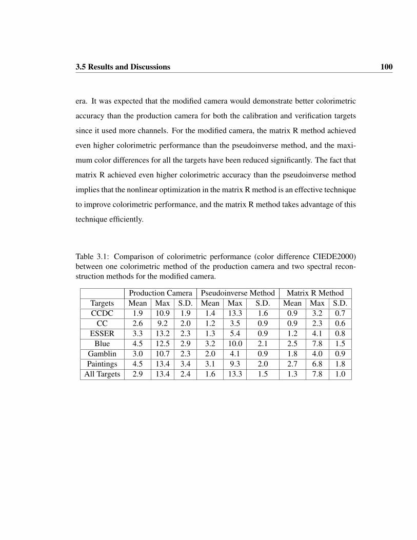
3.5 Results and Discussions 100
era. It was expected that the modified camera would demonstrate better colorimetric
accuracy than the production camera for both the calibration and verification targets
since it used more channels. For the modified camera, the matrix R method achieved
even higher colorimetric performance than the pseudoinverse method, and the maxi-
mum color differences for all the targets have been reduced significantly. The fact that
matrix R achieved even higher colorimetric accuracy than the pseudoinverse method
implies that the nonlinear optimization in the matrix R method is an effective technique
to improve colorimetric performance, and the matrix R method takes advantage of this
technique efficiently.
Table 3.1: Comparison of colorimetric performance (color difference CIEDE2000)between one colorimetric method of the production camera and two spectral recon-struction methods for the modified camera.
Production Camera Pseudoinverse Method Matrix R MethodTargets Mean Max S.D. Mean Max S.D. Mean Max S.D.CCDC 1.9 10.9 1.9 1.4 13.3 1.6 0.9 3.2 0.7
CC 2.6 9.2 2.0 1.2 3.5 0.9 0.9 2.3 0.6ESSER 3.3 13.2 2.3 1.3 5.4 0.9 1.2 4.1 0.8
Blue 4.5 12.5 2.9 3.2 10.0 2.1 2.5 7.8 1.5Gamblin 3.0 10.7 2.3 2.0 4.1 0.9 1.8 4.0 0.9Paintings 4.5 13.4 3.4 3.1 9.3 2.0 2.7 6.8 1.8
All Targets 2.9 13.4 2.4 1.6 13.3 1.5 1.3 7.8 1.0

3.5 Results and Discussions 101
CCDC CC ESSER Blue Gamblin Paintings All Targets0
1
2
3
4
5C
olor
diff
eren
ce, C
IED
E20
00
Color target
Production Camera Pseudoinverse Method Matrix R Method
Figure 3.2: Comparison of average CIEDE2000 color difference between one colori-metric method of the production camera and two spectral reconstruction methods forthe modified camera.
Tables 3.2 and 3.3 summarize the spectral performance metrics of the pseudoin-
verse and matrix R methods, including %RMS (root-mean-square) error and a metameric
index that consists of a parameric correction (Fairman, 1991) for illuminant D65 fol-
lowed by a CIEDE2000 color difference under Horizon illuminant with a correlated
color temperature near 2,200K. Horizon was used since it is a common light source
in museums. Because these two methods share the same metameric blacks obtained
from the spectral transformation, the statistical results for the metameric index are, by
definition, identical for these two methods. This level of performance is typical of this
multi-filter RGB approach (Berns, 2005a).

3.5 Results and Discussions 102
Table 3.2: Spectral performance metrics comparing a conventional small aperturein-situ spectrophotometer with the predicted spectral image using the pseudoinversemethod.
RMS (%) Metameric IndexTargets Mean Max S.D. Mean Max S.D.CCDC 1.6 4.0 0.6 0.7 7.6 1.0
CC 1.6 2.6 0.6 0.4 2.0 0.5ESSER 1.9 6.8 1.0 0.5 5.1 0.6
Blue 3.6 10.0 2.1 1.4 7.3 1.6Gamblin 2.8 8.5 1.5 0.6 2.4 0.6Paintings 2.9 8.8 1.7 1.1 8.9 1.9
All Targets 2.0 10.0 1.2 0.7 8.9 1.0
Table 3.3: Spectral performance metrics comparing a conventional small aperture in-situ spectrophotometer with the predicted spectral image using the matrix R method.
RMS (%) Metameric IndexTargets Mean Max S.D. Mean Max S.D.CCDC 1.5 3.9 0.6 0.7 7.6 1.0
CC 1.6 2.6 0.6 0.4 2.0 0.5ESSER 1.9 6.8 1.0 0.5 5.1 0.6
Blue 3.5 10.0 2.1 1.4 7.3 1.6Gamblin 2.8 8.5 1.5 0.6 2.4 0.6Paintings 2.9 8.7 1.7 1.1 8.9 1.9
All Targets 2.0 10.0 1.2 0.7 8.9 1.0
In theory, the matrix R method should decrease spectral accuracy since tristimu-
lus integration weights poorly approximate complex-subtractive colorants (Cohen and
Kappauf, 1985). As the differences in tristimulus values increase between the two fun-
damental stimuli, the spectral differences become more pronounced. In this research,
the matrix R method had minimal impact on spectral performance. This is likely a
result of the unconstrained nature of the spectral transformation and the sub-sampling

3.5 Results and Discussions 103
of the visible spectrum with six channels resulting in spectra that are already spectrally
selective. Furthermore, the tristimulus differences were not large. As a consequence,
the spectral properties were not adversely affected. For example, the measured and
predicted reflectances from these two methods for patch no.13 (blue) of the Gretag-
Macbeth ColorChecker are plotted in Figure 3.3. The estimated spectrum from the
pseudoinverse method undulates more than the measured spectrum. The matrix R
method did not add further undulation. In this particular case, spectral performance
improved. The value of the matrix R method is obvious when the color differences
are compared between measured and predicted reflectances for the pseudoinverse and
matrix R methods, 3.2 and 0.8, respectively. For this spectral imaging system, incorpo-
rating the fundamental stimuli from the optimized tristimulus values into the predicted
reflectance factors from the pseudoinverse method did not diminish the spectral per-
formance, but improved the colorimetric accuracy for a defined reference condition of
illuminant and observer.

3.5 Results and Discussions 104
400 450 500 550 600 650 700 0
0.05
0.1
0.15
0.2
0.25
0.3
0.35
Wavelength, nm
Ref
lect
ance
Fac
tor
Measured Pseudoinverse Method Matrix R Method
Figure 3.3: Comparison of measured reflectance factor (solid line) with predicted onesfrom the pseudoinverse method (dashed line) and matrix R method (dash-dotted line).
Two small oil paintings were also tested; one is a fish on a plate and the other is
a bouquet of flowers in a blue vase. Figure 3.4 is the sRGB representation of the re-
constructed multispectral image of the flower oil painting for CIE illuminant D65. The
eleven points are also marked locating the pure pigments used to create this painting.
The measured and predicted spectral reflectance factors for the nine chromatic pig-
ments using the matrix R method are plotted in Figure 3.5. For most of the pigments,
the estimated spectra capture the dominant spectral characteristics with more spectral
undulation. The exception is cobalt blue where the estimated spectrum is poor. Since
the matrix R method is a learning-based reconstruction method, the performance will
depend on the calibration target to a great extent. Recall that the ColorChecker DC was
used as the calibration target. This target does not contain pigments with long wave-

3.5 Results and Discussions 105
length reflectance tails. In fact, the main pigment used to create blue green and blue
colors is phthalocyanine blue, a cyan pigment whose reflectance factor is low through-
out the red region of the spectrum. Evaluating Table 3.3, there are two categories of
performance. The first is the CCDC, CC, and ESSER targets, having average %RMS
performance under 2.0. These targets do not contain blue colorants with long wave-
length tails. The second category is the Blue, Gamblin, and Paintings targets, having
average %RMS performance near 3.0. All of these targets contain pigments with long
wavelength tails including cobalt blue and ultramarine blue. For this reason, it is a
current research topic to develop a comprehensive calibration target that can cover the
spectral variability of all typical artist paints (Mohammadi et al., 2004a; Mohammadi
et al., 2005).

3.5 Results and Discussions 106
Figure 3.4: The sRGB representation of the reconstructed multispectral image of asmall oil painting with eleven marked spots made up of different pure pigments.1: Indian Yellow 2: Cadmium Yellow Medium 3: Phthalocyanine Green4: TiO2 White 5: Ivory Black 6: Phthalocyanine Blue7: Cobalt Blue 8: Cadmium Red Medium 9: Chromium Oxide Green10: Quinacridone Red 11: Venetian Red

3.6 Conclusions 107
400 500 600 700 0
0. 2
0. 4
0. 6
0. 8
1
Wavelength, nm
Ref
lect
ance
Fac
tor
Cadmium Yellow Medium
400 500 600 700 0
0. 2
0. 4
0. 6
0. 8
1
Wavelength, nm
Ref
lect
ance
Fac
tor
Indian Yellow
400 500 600 700 0
0. 2
0. 4
0. 6
0. 8
1
Wavelength, nm
Ref
lect
ance
Fac
tor
Phthalocyanine Green
400 500 600 700 0
0. 2
0. 4
0. 6
0. 8
1
Wavelength, nm
Ref
lect
ance
Fac
tor
Phthalocyanine Blu e
400 500 600 700 0
0. 2
0. 4
0. 6
0. 8
1
Wavelength, nm
Ref
lect
ance
Fac
tor
Cobalt Blue
400 500 600 700 0
0. 2
0. 4
0. 6
0. 8
1
Wavelength, nm
Ref
lect
ance
Fac
tor
Cadmium Red Medium
400 500 600 700 0
0. 2
0. 4
0. 6
0. 8
1
Wavelength, nm
Ref
lect
ance
Fac
tor
Chromium Oxide Green
400 500 600 700 0
0. 2
0. 4
0. 6
0. 8
1
Wavelength, nm
Ref
lect
ance
Fac
tor
Quinacridone Red
400 500 600 700 0
0. 2
0. 4
0. 6
0. 8
1
Wavelength, nm
Ref
lect
ance
Fac
tor
Venetian Red
Figure 3.5: Measured (solid line) and predicted (dashed line) spectral reflectance fac-tors using the matrix R method.
3.6 Conclusions
The image acquisition system, a modified commercial digital camera coupled with
two filters, is a simple and practical spectral imaging system. This image system was
tested with a new reconstruction method, the matrix R method. The new method is a
learning-based reconstruction method, which depends on the calibration target. The
method combines the benefits of both colorimetric and spectral transformations based
on the Wyszecki hypothesis, where any stimulus can be decomposed into a fundamen-

3.6 Conclusions 108
tal stimulus and a metameric black. The colorimetric transformation is nonlinearly
optimized to minimize the weighted color difference between measured and predicted
tristimulus values for a certain viewing condition, and the predicted tristimulus val-
ues are used to form the fundamental stimulus. The spectral transformation is linearly
optimized to minimize spectral RMS error between measured and predicted spectral
reflectance factors, and the predicted spectral reflectance factor is used to calculate the
metameric black. The final spectral reflectance factor combines the fundamental stim-
ulus from the colorimetric transformation and the metameric black from the spectral
transformation. The matrix R method takes advantage of both these transformations
efficiently. Combining the fundamental stimuli from optimized tristimulus values with
the predicted reflectances will not change the spectral performance, but can improve
the colorimetric accuracy significantly for a certain viewing condition. The nonlinear
optimization in the matrix R method is an effective technique to improve colorimetric
performance. The method can achieve reasonable spectral accuracy, and at the same
time higher colorimetric performance for a typical viewing condition. So it is a very
promising method for building digital image databases for museums, archives and li-
braries.
There are several opportunities for improvement. The first is to replace the tristim-
ulus integration weights used as additive primaries with primaries that better represent
complex-subtractive colorants, as demonstrated by (Li and Berns, 2007). Matrix R is
generalized as matrix S, [Eq. (3.7)], and matrix R method is defined by Eq. (3.14).
Rc = E (A′E)−1
T +(I− E (A′E)
−1A′
)N (3.14)
A second opportunity is to improve upon the pseudoinverse transformation where
the metameric black is estimated. One could constrain the transformation to improve

3.6 Conclusions 109
smoothness, use a different optimization technique such as the Weiner inverse, or add
a second step where the estimated spectrum is matched using apriori knowledge of the
objects colorants. This was demonstrated for artist paints and the use of Kubelka-Munk
turbid media theory as the mixing model (Zhao et al., 2005b). This approach combined
with image segmentation may enable the determination of concentration maps for each
colorant used in a work of art. This is a current area of research (Zhao et al., 2006).

Chapter 4
Pigment Mapping for Opaque
Materials
4.1 Introduction
The use of Kubelka-Munk turbid media theory (abbreviated as K-M theory) for col-
orant formulation has a long history, from the early days of calculators up to today’s
computer color-matching prediction. In most cases, pigmented materials are applied
to full opacity, so the simplified form of K-M theory for opaque materials can be used.
The reflectance of an opaque layer depends only on the ratio of absorption to scat-
tering coefficient and not on their absolute values. On the other hand, in other cases,
pigmented materials are not applied to full opacity, so the general form for translu-
cent materials should be used. The reflectance of a translucent layer depends on the
thickness of the layer, the reflectance of backing, both absorption and scattering coeffi-
cients. The focus of this chapter is opaque materials, and the translucent materials will
be discussed later.

4.1 Introduction 111
The pigment-mixing model describes the mathematical relationship between the
input to a coloration system (e.g., the concentrations of the constituent pigments of
a mixture) and the output (e.g., spectral reflectance or colorimetric coordinates of a
mixture). The spectral reflectance of a mixture is nonlinearly related to the concen-
trations of its constituent pigments, while both absorption and scattering coefficients
are linearly related to these concentrations (Duncan, 1949). For single-constant the-
ory, it is assumed that the scattering coefficient of white paint such as titanium dioxide
white is dominant, i.e., adding small amount of colored pigment to white paint does
not affect its scattering capacity (Allen, 1980). So the ratio between absorption and
scattering for a mixture depends on the ratios of its constituent pigments and their rel-
ative concentrations. For single-constant theory, only one parameter per wavelength,
the ratio of absorption to scattering coefficient, is needed to characterize a pigment.
A detailed discussion of single-constant theory can be found in the reference (Berns
and Mohammadi, 2007b). The reference (Mohammadi and Berns, 2004) concluded
that one mixture sample of a pigment with white paint near the maximum chroma was
the best choice to characterize the pigment. However, the accuracy of single-constant
theory is limited. One main reason is that the ratio between absorption and scattering
coefficients for a mixture does not linearly rise as the increase of the pigment concen-
tration. So it is necessary to require five or more mixture samples with white paint in a
tint ladder in order to describe this nonlinearity. Another reason is that the assumption,
where the scattering power of each sample is considered to be equal to that of white
paint, might be invalid. So two-constant theory is used, and for each wavelength, two
parameters – both absorption and scattering coefficients – are needed to characterize
each pigment in the database.
Building a pigment database is the first and most important component of any

4.2 Database Development 112
color-matching system. For two-constant theory, the database consists of the pigment
constants - both absorption and scattering coefficients - for each and every pigment
in the database. The performance of color-matching prediction system critically relies
on the accuracy of the pigment constants. Given a spectral reflectance of a mixture,
the question is to find its constituent pigments and quantify their concentrations. For a
simple patch, it is to acquire its colorant formula or recipe based on in situ spectropho-
tometric measurement, while for a complex image (e.g., a painting), it is to obtain
spatial concentration maps of pigments consisting of the painting based on multispec-
tral imaging.
In this chapter, the database development for opaque materials is considered in
section 4.2. The color-matching prediction for simple patch based on in situ spec-
trophotometry is dealt with in section 4.3, and the pigment mapping for a complex
image based on spectral imaging is discussed in section 4.4. Finally, a summary is
given in section 4.5.
4.2 Database Development
4.2.1 Methods
For two-constant theory, the pigment constants including both absorption and scatter-
ing coefficients need to be determined for each pigment. The accuracy of the pigment
constants is very important for color-matching prediction. Both the absorption and
scattering coefficients can be determined from at least two paint samples of the pig-
ment. Two samples can reach a unique solution of the unit absorption and scattering
coefficients for the pigment. If more than two samples are prepared, the pigment con-
stants are optimized using the linear least square (LLS) method for each wavelength

4.2 Database Development 113
(Walowit et al., 1988). As the number of pigments in the database increase, it is labori-
ous and onerous to prepare a larger number of paint samples. In order to alleviate this
issue, it is beneficial to prepare just two paint samples for each pigment in the database
in order to characterize it. In a previous MCSL report (Mohammadi and Berns, 2004),
it was concluded that the best two samples are one masstone sample and one mixture
sample with white paint, near the maximum chroma. To bypass the trouble of prepar-
ing the mixture sample with the maximum chroma, the reference (Zhao and Berns,
2006) concluded that the optimal colorant concentration for the calibration mixture is
between 40% and 60%, in the neighborhood of maximum chroma.
4.2.1.1 Characterization of White Paint
For opaque materials, the pigment constants can be determined on a relative basis. It
is assumed that the scattering coefficient of white pigment sw is equal to unity at all
wavelengths, where the subscript w refers to the white pigment. All other absorption
and scattering coefficients are expressed relative to sw. The titanium dioxide white
is used to mix with the colored pigments because of its high scattering power. This
approach does not require the absolute value of sw, and can give very satisfactory
results when the samples are applied to full opacity (i.e., opaque at all wavelengths).
At least one sample of the white paint is required to obtain its absorption coefficient
kw. Since sw is equal to unity at all wavelengths, kw is equal to the(
KS
)w
, calculated
from measured spectral reflectance after Saunderson correction.
The sample is measured with an integrating spectrophotometer with spectral com-
ponent included, which is recommended by McDonald (McDonald, 1987). Although
the mode of measurement with spectral component excluded is the nearest to that of
the human observer, it is the least suitable for color-matching prediction for pigment

4.2 Database Development 114
materials. One possible reason is because small blemishes, fingerprints, scratches and
gloss effect might cause the variation in reflectance. Another reason is that variable
amounts of specular component are always included since no samples of pigment ma-
terials are perfectly optically flat. This results in poor measurement repeatability and
consequently poor pigment database for color-matching prediction. For this reason,
total reflectance factor, measured with an integrating sphere with spectral component
included, is preferred for color-matching prediction.
4.2.1.2 Characterization of Other Paints
After that, the pigment constants for the other pigments can be determined. For each
pigment, at least two samples one pure pigment or masstone and one mixture sample
with white paint are needed to characterize this pigment. The spectral reflectance
factors of these two samples were obtained and corrected by the Saunderson Equation.
Then the ratios between absorption and scattering coefficients(
KS
)mass
and(
KS
)mix
are
calculated from the corresponding corrected reflectances, where the subscripts mass
and mix refer to the masstone and mixture samples respectively. The small k and s
means the absorption and scattering coefficients all at unit concentration. For masstone
sample, small k and s is the same as capital K and S in Eq. (4.1). For a mixture
sample, the ratio(
KS
)mix
can be further expressed as summation of unit absorption
coefficients of its component pigments, weighted by corresponding concentrations,
divided by summation of unit scattering coefficients, as shown in Eq. (4.2).
(K
S
)mass
=k
s(4.1)
(K
S
)mix
=ck + (1− c)kw
cs + (1− c)sw
(4.2)

4.2 Database Development 115
Then the unit absorption and scattering coefficients for the pigment of interest, can
be resolved directly from(
KS
)mass
for masstone sample,(
KS
)mix
for mixture sample,
kw and sw for white paint and the pigment concentration c in mixture sample. The
constants can be calculated for each and every wavelength using Eqs. (4.4) and (4.3).
s =1− c
c
(KS
)mix
sw − kw(KS
)mass
−(
KS
)mix
(4.3)
k = s
(K
S
)mass
(4.4)
4.2.1.3 Further Simplification
For each pigment, two characterization samples need to be prepared. One is 100% pure
pigment, and the other is a mixture of the pigment and white paint. The procedure can
be further simplified if weight measurement can be omitted when making the mixture
sample. It is found that the uncertainty in the pigment concentration of the characteri-
zation mixture sample will cause slight uncertainty in the predicted concentrations for
test mixture samples, but will not affect the spectral accuracy of predicted reflectance
factors at all. Although the predicted colorant recipe or formulation is not so accurate,
batch correction can be used as a post-process step to slightly adjust the recipe. The
procedure of preparing paint samples to characterize each pigment in a database can be
greatly simplified if the pigment and white paint can be mixed roughly at 1:1 without
weighting. As the number of pigments to be characterized increases dramatically, the
benefit of the simplified procedure without weighting is more pronounced. The gain
in the simplified procedure of database preparation will compensate somewhat inaccu-
racy in the predicted recipe. The detailed mathematical proof will be provided next.
Both the absorption and scattering coefficients, k and s, can be decomposed into

4.2 Database Development 116
two parts - basic spectra, k0 and s0, and a scaling factor 1−cc
. If pigment concentration
of the characterization mixture sample is unknown and arbitrarily set to c, the basic
spectra for both absorption and scattering coefficients can still be calculated, and the
scaling factor is however uncertain.
k =1− c
ck0 (4.5)
s =1− c
cs0 (4.6)
k0 = s0
(K
S
)mass
(4.7)
s0 =
(KS
)mix
sw − kw(KS
)mass
−(
KS
)mix
(4.8)
Given a test mixture sample, made up of one pigment and white paint, the ratio(KS
)t
can be calculated from reflectance factor for this sample. The constants kw and
sw for white paint are known, and the constants k and s for the pigment of interest are
calculated from Eqs. (4.5) and (4.6) assuming the concentration of the characterization
pigment mixture is c. Then the concentration of the test mixture sample ct is the only
unknown in Eq. (4.9). (K
S
)t
=ctk + (1− ct)kw
cts + (1− ct)sw
(4.9)
The above equation can be rewritten as Eq. (4.10) for each wavelength.
−[(
K
S
)t
s− k
]=
1− ct
ct
[(K
S
)t
sw − kw
](4.10)
The ratio 1−ct
ctcan be calculated based on linear least squares (LLS) method. For a
linear equation y = a + bx, the optimal solution for the slope is equal to ssxy
ssxx, where

4.2 Database Development 117
ssxy is covariance of two variables x and y and ssxx is variance of the variable x. So
assume the number of wavelength is n, the ratio 1−ct
ctcan be expressed as shown in Eq.
(4.11), where xi =[(
KS
)t,i
sw,i − kw,i
]and ct is the optimal solution of LLS method.
1− ct
ct
=−
∑ni=1 xi
[(KS
)t,i
si − ki
]+ 1
n
∑ni=1 xi
∑ni=1
[(KS
)t,i
si − ki
]∑n
i=1 x2i
(4.11)
Eq. (4.11) can be rewritten as followings,
1− ct
ct
=1− c
cA (4.12)
A =−
∑ni=1 xi
[(KS
)t,i
s0,i − k0,i
]+ 1
n
∑ni=1 xi
∑ni=1
[(KS
)t,i
s0,i − k0,i
]∑n
i=1 x2i
(4.13)
Then the ratio ˆ(KS
)t
can be calculated from the predicted concentration for the test
sample.ˆ(
K
S
)t
=k0 + Akw
s0 + Asw
(4.14)
Several conclusions can be drawn based on the above derivation.
• The unit absorption and scattering coefficients k and s of the pigment of interest
have the same scaling factor 1−cc
, where c is the concentration of the charac-
terization mixture sample. If c is unknown, their basic spectral curves can be
determined with k0 and s0, and the absolute values can be obtained by the same
scaling factor [Eqs. (4.5) and (4.6)].
• The predicted concentration ct for a test mixture sample relies on the concentra-
tion of the characterization mixture sample [Eq. (4.12)].
• The estimated ratio between the absorption and scattering coefficients for the test

4.2 Database Development 118
mixture sample ˆ(KS
)t
is independent on the concentration of the characterization
mixture sample [Eq. (4.14)].
If the concentration of the characterization mixture is unknown, the scaling factor
in Eqs.(4.5) and (4.6) is unspecific. However, since the factor is combined with the
pigment concentration in Eq.(4.9), it will only affect the accuracy of the predicted
concentration ct, but not the spectral accuracy of ˆ(KS
)t. Discussion so far assumes that
the test mixture sample is made up of only one pigment and white paint. The same
conclusion can easily be drawn for any test mixture sample consisting of more than
one pigment and white paint.
In summary, the unit k and s for each pigment can be calculated based on two
samples - one masstone and one mixture sample. If the mixture sample has pigment
concentration near 50%, the procedure of database development can be greatly sim-
plified. These pigment constants can be used in color-matching prediction. The ratioˆ(
KS
)t
for the other test mixture sample of the same pigment is independent of the con-
centration of the characterization mixture sample. The predicted colorant recipe or
formulation might not be accurate without knowledge of the concentration of the char-
acterization mixture sample, batch correction can be used as post-processing step to
slightly adjust the recipe.
4.2.2 Experimental
Samples of Golden Acrylic Artist Colors were carefully prepared by one of our group
members. There are in total 28 colorants plus white paint. All these samples were mea-
sured by an integrating-sphere spectrophotometer with spectral component included.
For each colorant, there were at least six mixture samples with white paint at about
0%, 20%, 40%, 60%, 80% and 100% colorant concentrations. The unit absorption and

4.2 Database Development 119
scattering coefficients for each colorant were calculated based on white paint, masstone
and a mixture sample at a certain concentration, shown as Eqs. (4.4) and (4.3). After
that, the concentrations for all the mixture samples with white paint were predicted
using linear least squares method, shown as Eq. (4.11). Finally, the ratios between
absorption and scattering coefficients for all these samples were reconstructed using
the predicted concentrations, shown as Eq. (4.14). It is also worth mentioning that
the Saunderson equation was used to transform measured reflectance into internal re-
flectance, used in two-constant K-M theory. The two parameters in the Saunderson
equation were 0 and 0.6 (Okumura, 2005).
4.2.3 Results and Discussions
As discussed earlier, the goodness of fit between ˆ(KS
)t
and(
KS
)t
is independent of the
concentration of the characterization mixture sample. As a result, the spectral and col-
orimetric accuracies of reconstructed reflectance factor should be identical no matter
what the concentration is assumed for the characterization mixture sample. However,
prediction of the concentration from a test mixture sample relies critically on knowl-
edge of the concentration of the characterization mixture sample, which if unknown
should be estimated as accurately as possible.
Spectral and colorimetric accuracies of the proposed approach by comparing recon-
structed reflectance factors with spectrophotometer measurements are listed in Table
4.1. For each colorant, the mixture sample of certain colorant concentration was used
as the calibration sample along with the corresponding masstone to predict reflectance
factor for all the mixture samples of the same colorant. This procedure was repeated
for all the colorants and spectral and colorimetric performance metrics based on all
mixture samples were calculated. For example, if all the calibration mixture samples

4.2 Database Development 120
had 20% colorant concentration, the mean and maximal RMS errors were 0.52% and
2.92% respectively. The maximum chroma means that for each colorant, the calibra-
tion mixture sample was chosen so that it exhibited the highest chroma among all the
mixture samples of the same colorant, unless it happened to be the masstone, in which
case, the mixture sample with the second highest chroma was selected, instead.
Table 4.1: Spectral and colorimetric accuracies of reconstructed reflectance factorscompared with in situ spectrophotometer measurements.
Mixture RMS (%) Color Difference ∆E00 (D65, 2o)Concentration Mean Max 90% Mean Max 90%
(Mass, %) Percentile Percentile20 0.52 2.92 1.48 0.34 2.28 0.8840 0.32 1.56 0.84 0.23 1.73 0.5960 0.34 1.94 0.84 0.26 2.59 0.6080 0.47 3.87 1.34 0.36 3.49 0.77
Max Chroma 0.36 1.94 0.90 0.25 1.53 0.70
Both spectral and colorimetric accuracies improved initially as the concentration of
the calibration mixture sample increased, and then declined as the increase continued.
It can also be seen that the performance of the calibration mixture sample with 40%
– 60% colorant concentration is comparable to that of the sample with the maximum
chroma. This simplification can facilitate building the colorant database.
4.2.4 Summary
This section focused on determining the minimum number of samples in order to char-
acterize a pigment’s optical properties and which amounts to determination of its unit
absorption and scattering coefficients using two-constant K-M theory. Two calibration
4.2 Database Development 121
samples, a pure pigment (masstone) and a mixture sample of unknown colorant con-
centration with white paint, were sufficient to obtain both unit absorption and scattering
coefficients of the colorant but their absolute levels might be off by the same scaling
factor. When they are used to analyze an unknown mixture sample, such uncertainty
in their absolute levels will influence prediction of colorant concentration but does
not affect the spectral and colorimetric accuracies of reconstructed reflectance factor.
Therefore, pigment identification can still be achieved. Since the weight measurement
for determination of colorant concentration is no longer necessary, preparation of cali-
bration mixture sample becomes much easier and more convenient. On the other hand,
if the colorant concentration of the calibration mixture sample is known, the absolute
levels of the unit absorption and scattering coefficients of the colorant can be obtained
and pigment mapping is realized since accurate prediction of colorant concentration
for the unknown mixture sample becomes possible. The optimal colorant concentra-
tion was found to be between 40% and 60% for the calibration sample, which gave
comparable performance for prediction of unknown mixture sample as that provided
by the concentration that has the maximum chroma. Finally, compared with the con-
ventional approach based on a tint ladder consisting of at least five mixture samples,
this research indicates that two calibration samples are sufficient to characterize each
colorant, which greatly simplifies the process to develop a colorant database. This ap-
proach is only sufficiently accurate to predict concentration for the purpose of pigment
mapping, but not for precise recipe prediction. Industrial practice might still require
more samples to characterize a colorant database and batch correction to improve ac-
curacy of recipe prediction.

4.3 Colorant Formulation for Simple Patches 122
4.3 Colorant Formulation for Simple Patches
4.3.1 Pigment Database
The first and most important step of any color-matching prediction is to characterize
the optical properties of each pigment forming the database. Four Golden acrylic matte
fluid paints were used in this experiment, and they are titanium dioxide white, hansa
yellow opaque, pyrrole red and ultramarine blue. These paints were premixed with
other mediums and additives. The scattering coefficient of white paint was set to unity
at all the wavelengths, and its absorption coefficient was calculated from measured
reflectance factor of 100% pure white paint after Saunderson correction. The other
paints were characterized using masstone-tint method for the opaque case.
The absorption and scattering coefficients of all four paints are plotted in Figure
4.1. The scattering coefficient spectrum for hansa yellow opaque at longer wavelengths
(between 500nm and 700nm) were unsmooth. The main reason was that the difference
of reflectance factors between masstone and mixture samples, which were used to
characterize this paint, were less than 0.05, as shown in reference (Okumura, 2005).
It is stated in (Nobbs, 1997) that the precision of the optical constants (absorption
and scattering coefficients) depends on the precision of measurement of reflectance
factors, and the errors of the optical constants increase rapidly as reflectance factor of
mixture sample approaches either reflectance factor of white paint or masstone sample.
The same reason can be used to explain for the unsmoothness of scattering coefficient
spectrum of pyrrole red.

4.3 Colorant Formulation for Simple Patches 123
360 460 560 660 7600
1
2
3
4
5
Wavelength, nm
Uni
t Abs
orpt
ion,
kTitanium whiteHansa YellowPyrrole RedUltramarine Blue
(a) Absorption Coefficient
360 460 560 660 7600
0.4
0.8
1.2
Wavelength, nm
Uni
t Sca
tterin
g, s
(b) Scattering Coefficient
Figure 4.1: Absorption and scattering coefficients for four Golden acrylic paints.
4.3.2 Color-Matching Prediction
The second step is to select the set of paints that matches the standard according to
user-defined criteria such as spectral similarity, color difference under one or more il-
luminants, metamerism and cost. Since there were only four paints in the database, it
was first assumed that any test mixture sample was made up of all four paints. The four
concentrations were optimized to minimize the weighted spectral RMS error, wRMS,
shown in Eq. (4.15), between measured Rλ and predicted Rλ reflectance factors. The
weighted RMS error weighted spectral data with small magnitude more than the ones
with large magnitude, because human vision system is more sensitive to mismatch in
dark colors than light colors. The concentrations were fully constrained, i.e., each con-
centration was between zero and one, and the sum of four concentrations was equal to
one. Sequential quadratic programming was used to optimize the four concentrations.
The paint was removed from the composition if its concentration was less than 5%

4.3 Colorant Formulation for Simple Patches 124
based on some prior knowledge.
wRMS =
√√√√∑nλ=1
[√1
Rλ
(Rλ − Rλ
)]2
n(4.15)
The test target was a custom target, made up of four golden acrylic matte fluid
paints, and abbreviated as the Golden target in the following discussion. There were
forty-five patches in this target, shown in Figure 4.2. The first eighteen patches (the 1st
and 2nd rows) were tint ladders of these three colored paints. The next nine samples
(the 3rd row) were mixtures of two colored paints without white paint, and the last
eighteen samples (the 4th and 5th rows) were mixtures of two colored paints with white
paint. All these samples were carefully prepared and measured using an integrating
sphere spectrophotometer with spectral component included.
Figure 4.2: Forty-five patches of Golden Target.
The error metric of colorant formulation was the squared Euclidean distance be-
tween the known and predicated recipes. The statistical results for this error metric for
colorant formulation are listed in Table 4.2. The program successfully identified the

4.3 Colorant Formulation for Simple Patches 125
paints except for white paint within each patch and determined their concentrations.
The mean concentration error was 3.1%, but the maximum error was 15.7%. It was
found that the errors were high for two colorant mixtures without white paint, corre-
sponding to patch Nos. 19-27 (the 3rd row of Golden Target). It might be caused by
the accuracy of two-constant Kubelka-Munk theory or a lack of opacity for the paint
samples. The existence of white paint improved the accuracy of the concentration
determination. If patch Nos. 19-27 were excluded, the mean error reduced to 1.0%,
indicating a very successful pigment mapping.
Table 4.2: Statistical results of concentration error for colorant formulation (%).
Statistics Mean Std. 90% percentile Min MaxAll patches 3.1 4.6 11.0 0.0 15.7
Excluding PatchesNos.19-27 (3rd row) 1.0 1.2 1.9 0.0 5.1
The spectral reflectance factors were estimated from both the known and optimized
recipes. Measured and estimated spectral reflectance factors with the spectral RMS
errors included in the legend were plotted in Figure 4.3. Compared with measured re-
flectance factor, two estimated reflectance spectra were more jagged. It was caused by
the inaccuracy of pigment database. This patch was made up of hansa yellow opaque
and ultramarine blue. The scattering coefficient of hansa yellow opaque at longer
wavelength (between 500nm and 700nm) was unsmooth, shown in Figure 4.2, which
caused the jagged shape of estimated reflectance spectra. The optical properties of the
yellow paint was calculated based on two calibration samples – one 100% pure paint
and one mixture of the paint with titanium dioxide white. The low accuracy of the
optical properties for the yellow paint might be improved when one mixture sample of
the yellow paint with a small amount of black paint was used to characterize it. The

4.3 Colorant Formulation for Simple Patches 126
estimated spectral reflectance from the optimized recipe had a smaller spectral RMS
error than that from the known recipe. This was expected since the optimized recipe
was optimized to minimize the weighted RMS error between the measured and esti-
mated spectral reflectance factors. Noticeable discrepancies were observed between
the measured and estimated spectral reflectance factors from the known recipe. Such
discrepancy might be caused by the accuracy of the Kubelka-Munk model. Other pos-
sible reasons might include measurement error, lack of opacity, non-uniformity of the
paint sample, and numerical error.
380 430 480 530 580 630 680 7300
0.05
0.1
0.15
0.2
0.25
0.3
0.35
Wavelength, nm
Ref
lect
ance
Fac
tor
Patch No. 20
Measurement
Known recipe RMS = 6.3%
Predicted recipe RMS = 1.8%
Figure 4.3: Measured spectral reflectance factor (solid line) and estimated spectralreflectance factors using the known (dashed line) and optimized (dash-dotted line)recipes of Patch No. 20 of Golden Target.
4.3.3 Summary
The first and most important step of any color-matching prediction is to characterize
the optical properties of each pigment forming the database. When samples are ap-
plied to full opacity, the optical constants - absorption and scattering coefficients - can

4.3 Colorant Formulation for Simple Patches 127
be calculated on a relative basis, i.e., the scattering power of white paint, sw is set to
unity at all the wavelengths, and the other optical constants are all relative to sw. To
simplify the procedure of database development, it is necessary to reduce the number
of paint samples for each paint to be characterized. The masstone-tint method was
used to characterize each and every paint with only two samples - one was a masstone
sample and the other was a mixture sample with white paint. The accuracy of these
optical constants were tested in color-matching prediction.
The second step is to select a set of paints that matches the standard according
to user-defined criteria such as spectral similarity, color difference under one or more
illuminants, metamerism and cost. The criterion was the weighted spectral RMS er-
ror between measured and predicted reflectance factors, which weighted spectral data
with small magnitude more than the ones with large magnitude since the human vision
system is more sensitive to mismatches in dark colors than light colors. The program
successfully identified the composite paints except for white paint in each patch and
determined their concentrations. The concentration error for paint mixtures without
white was higher than that for mixtures with white paint. It might be caused by the
invalidity of scalability assumption, limitation of two-constant theory, lack of opacity
for paint samples or weight measurement error. Since the white paint, e.g., titanium
dioxide white, has very high absorption, the existence of white paint generally im-
proves the accuracy of the concentration determination. The spectral reflectance factor
can be estimated from both the known and optimized recipes. The accuracy of pre-
dicted reflectance factors critically depended on the accuracy of the optical properties
of the pigments in the database. The estimated spectral reflectance from the optimized
recipe had a smaller spectral RMS error than that from the known recipe. Noticeable
discrepancies were observed between the measured and estimated spectral reflectance

4.4 Pigment Mapping for a Complex Image 128
factors from the known recipe. Such discrepancy might be caused by the accuracy of
the Kubelka-Munk model. Other possible reasons might include measurement error,
lack of opacity, non-uniformity of the paint sample, and numerical error.
4.4 Pigment Mapping for a Complex Image
4.4.1 Introduction
Spectral imaging techniques have been well developed in the last ten years for the art
conservation field. Spectral reconstruction algorithms have achieved sufficiently high
accuracy to predict specific pigments and their concentrations for each pixel on works
of art. Digital rejuvenation can be promptly performed on works of art based on the
pigment mapping to correct changed color or repaint discolored parts by simulation.
In this pilot experiment, a painting was made of ten Gamblin artist oil paints plus
white paint. A spectral image of the painting was derived from multi-channel camera
signals. To overcome the difficulty of unmixing a large spectral image, the image was
first segmented using k-Means classification in CIELAB color space. Within each
segmented region, based on its colorimetric property, a subgroup of pigments was
selected from a predefined pigment database. Pigment mapping was then implemented
for each pixel in this segmented region with this subgroup of pigments based on two-
constant Kubelka-Munk theory. By focusing on a subgroup of pigments rather than
unmixing with the entire pigment database for each pixel, the computation efficiency
was greatly improved.

4.4 Pigment Mapping for a Complex Image 129
4.4.2 Experimental
The input device of the spectral image acquisition system was a Sinarback 54H dig-
ital camera that has a Kodak KAF-22000CE CCD with a resolution of 5440 × 4880
pixels. The camera employed a color-filter-array (CFA) and a filter slider with two
customer-designed filters that improved both color and spectral accuracies over the
production camera (Taplin and Berns, 2005; Berns et al., 2005a; Berns et al., 2005b).
In each position of the filter wheel, a three-channel image was collected, producing
a six-channel camera image. A calibration target (GretagMacbeth ColorChecker DC)
was imaged by the camera and measured using a bidirectional spectrophotometer. A
reconstruction model was derived to convert the multi-channel camera data to spec-
tral reflectance data for each pixel (Zhao and Berns, 2007). The model consisted of
both colorimetric and spectral transformations, which achieved high spectral and col-
orimetric accuracies simultaneously for a certain viewing and illuminating condition.
Following camera calibration, spectral reflectance as a function of spatial position was
estimated for any imaged target.
For this experiment, the test target was a small oil painting, featured with flow-
ers in a blue vase, which was made using Gamblin artist oil paints. The following
paints were used: cadmium yellow medium, indian yellow, cadmium red medium,
venetian red, quinacridone red, phthalocyanine green, chromium oxide green, cobalt
blue, phthalocyanine blue, ivory black and titanium dioxide white. The detailed paint
information can be found in Appendix C.
4.4.3 Pigment Database
The pigment database for the Gamblin artist oil paints was developed in the same way
as the database for the Golden acrylic matte fluid paints. The scattering power of the

4.4 Pigment Mapping for a Complex Image 130
white paint was set to unity at all the wavelengths, and the optical properties of all the
other paints were calculated based on the masstone-tint method for the opaque case.
The detailed information for database development can be found in Appendix C. Berns
(Berns et al., 2002) suggested that the logarithm of the absorption and scattering ratio
was the most invariant to changes in concentration. The negative logarithm spectra
− log (K/S) of the ratio between absorption and scattering coefficients of these paints
were plotted in Figure 4.4.
380 430 480 530 580 630 680 730
10
8
6
4
2
0
-2
-4
Wavelength,nm
-Log
(K/S
)
Cadmium Yellow MediumIndian Yellow
Cadmium Red MediumVenetian RedQuinacridone RedPhthalocyanine GreenChromium Oxide GreenCobalt BluePhthalocyanine BlueIvory Black
Figure 4.4: The − log (K/S) spectra of ten gamblin artist oil paints
4.4.4 Image Segmentation
The spectral image of the test target was obtained from two raw camera RGB images
using the reconstruction method described in reference (Zhao and Berns, 2007). It
was then transformed to a CIELAB image for CIE illuminant D65 and the 2-degree
observer. The unsupervised k-Means clustering method was used to segment the

4.4 Pigment Mapping for a Complex Image 131
CIELAB image into five clusters in a*b* space. The k-means algorithm was discussed
in the book Pattern Classification (Duda et al., 2001). A brief introduction of this al-
gorithm follows. The only input to the algorithm is the number of clusters, k. First,
k initial centers are randomly selected from the whole data points. The next step is to
associate each data point to the nearest center and classified it into that cluster. After
all the data points are processed, the k new centers are recalculated based on the clas-
sified data points. The process is repeated until the centers do not move any more. The
clustering process was implemented by the kmeans function in MATLAB. The scatter
plot of the five segmented clusters in a*b* space is shown in Figure 4.5.
Figure 4.5: Scatter plot of five segmented clusters in a*b*space.
The original image and five segmented images are shown in Figure 4.6.The k-
Means clustering method successfully segmented the image based on colorimetric in-
formation. The number of clusters was determined to be five through trial-and-error.
Four clusters were insufficient to separate certain colors. On the other hand, six or
more clusters provided more detail than was necessary for the test target. Cluster 5

4.4 Pigment Mapping for a Complex Image 132
consists of all low chroma colors and locates near the center of a*b* space (Figure
4.5).
(a) Original (b) C1 Bluish (c) C2 Greenish
(d) C3 Yellowish (e) C4 Reddish (f) C5 Low Chroma
Figure 4.6: Original image of the oil painting and five segmented images.
4.4.5 Pigment Mapping
In this small oil painting, only a small portion consisted of pure pigments with the
majority being mixtures. Several assumptions were made: (1) the painting was totally
opaque; (2) most mixtures were made of only one chromatic pigment with white paint,

4.4 Pigment Mapping for a Complex Image 133
and some mixtures were made of no more than four chromatic pigments with white.
Because Cluster 5 was somewhat transparent and appeared to consist of more than four
pigments, it was eliminated from the following analysis.
For each cluster, several candidate pigments were selected based on colorimetric
information. As listed in Table 4.3, Cluster 1 contained two blue pigments. For Cluster
2, one yellow pigment was included along with two green pigments, as visual inspec-
tion of the painting indicated the existence of yellow among the dominant green colors.
The same conclusion applied to Clusters 3 and 4. The ivory black was not selected for
these four clusters since it might only exist in Cluster 5. After that, pigment mapping
was performed pixel-wise using the selected pigments for each cluster. The criterion
was to minimize the spectral reflectance factors estimated from the camera signals and
the pigment compositions for each pixel.
Table 4.3: Selected pigment combinations for each cluster.
Cluster NumberPaints 1 2 3 4
Cadmium Yellow Medium x xIndian Yellow x x
Cadmium Red Medium xVenetian Red x
Quinacridone Red xPhthalocyanine Green x
Chromium Oxide Green x xCobalt Blue x
Phthalocyanine Blue xIvory Black
Nine points on the painting were selected and measured with a bidirectional spec-
trophotometer. For each point, reflectance spectra were estimated from both the camera

4.4 Pigment Mapping for a Complex Image 134
signals and pigment mapping. The estimated spectra from the camera signals and pig-
ment mapping along with the in situ spectrophotometer measurements for four chro-
matic pigments were plotted in Figure 4.7. It can be clearly seen that the estimated
reflectance spectra from pigment mapping were more accurate and much closer to the
in situ measurements. The same result has been obtained using simulated camera data
(Zhao et al., 2005a), discussed in the next chapter. It was concluded that the accuracy
of spectral imaging was high enough to predict specific pigments and their concentra-
tions for each pixel in the painting, and that by incorporating pigment information, the
accuracy of spectral image was further improved.
400 500 600 7000
0.2
0.4
Wavelength, nm
Ref
lect
ance
Fac
tor
Phthalocyanine Blue
(a) Phthalocyanine Blue
400 500 600 7000
0.2
0.4
Wavelength, nm
Ref
lect
ance
Fac
tor
Chromium Oxide Green
(b) Chromium Oxide Green
400 500 600 7000
0.5
1
Wavelength, nm
Ref
lect
ance
Fac
tor
Cadmium Yellow Medium
(c) Cadmium Yellow Medium
400 500 600 7000
0.5
1
Wavelength, nm
Ref
lect
ance
Fac
tor
Venetian Red
(d) Venetian Red
Figure 4.7: Measured (red solid line) and predicted spectral reflectance factors fromcamera model (black dash-dotted line) and pigment mapping (blue dashed line) forfour spots marked in the painting.

4.4 Pigment Mapping for a Complex Image 135
4.4.6 Summary
The CIELAB image of the test target was first segmented using K-Means classifica-
tion in a*b* color space. Within each cluster, a subgroup of candidate pigments was
selected from a ten- pigment database. After that, pigment mapping was implemented
on pixel basis using two-constant Kubelka-Munk theory to obtain a concentration map
for each pigment. This technique resulted in quite good performance. By focusing on a
subgroup of pigments rather than unmixing with the entire pigment database for each
pixel, the computation efficiency was improved greatly. It also proved that spectral
imaging techniques had the potential to identify pigments and determine their concen-
trations image-wise.
The fundamental basis of the technique presented in this section is the spectral ac-
curacy of the camera model. The choice of calibration target greatly affects estimation
accuracy and it is critical that the target should span both the spectral and colorimetric
description of the painting (Berns and Imai, 2002). Since the current calibration target
(ColorChecker DC) does not satisfy the above requirements, better spectral accuracy
should be expected with a more appropriate target (Mohammadi et al., 2005). It is also
possible to develop an automatic selection routine for candidate pigments instead of the
manual process used for this research. Finally, it is more common that the pigments
in a painting are unknown. This problem can be solved in two steps: (1) select candi-
date pigments from a larger database; and (2) mapping each pixel using the described
technique.

4.5 Conclusions 136
4.5 Conclusions
The use of Kubelka-Munk turbid media theory in predicting spectral reflectance fac-
tor of opaque specimen from the the specimen’s constituent optical properties is well
established and very successful in practice. Practical success has been achieved by the
reduction in mathematical complexity when the specimen is opaque and the elimina-
tion of controlling thickness.
The first and most important step for any color-matching system is to develop a pig-
ment database, which includes optical constants - absorption and scattering coefficients
- of each and every pigment in the database. As the number of pigments available in-
creases, it is tedious and time-consuming to prepare paint samples to characterize each
paint of interest. It was found that two calibration samples, one pure pigment (mas-
stone) and a mixture sample of this pigment with white paint in the neighborhood
of maximum chroma, were sufficient to obtain both absorption and scattering coeffi-
cients for this pigment. It greatly simplified the procedure of database development
since only two paint samples were required for each pigment. If the objective is to
simply find the composite pigments for an unknown mixture sample without need to
obtain its precise recipe, the weighting step can be omitted when making the calibra-
tion mixture samples. The absorption and scattering coefficients are off by the same
scaling factor. It was mathematically proven that the uncertainty in the concentration
of calibration mixture samples did not affect the accuracy of spectral prediction. Thus,
removing weighting further simplified the procedure of database development. The
inexact recipe can be tuned through the post-processing batch correction. Two opaque
pigment databases were developed using the simplified procedure but with weighting.
One included eleven Gamblin artist oil paints, and the other included twenty-eight
Golden acrylic matte fluid paints.

4.5 Conclusions 137
The second step was to select the set of paints that matched the standard accord-
ing to user-defined criteria such as spectral similarity, color difference under one or
more illuminants, metamerism and cost. The criterion was the weighted spectral RMS
error between measured and predicted reflectance factors. The colorant formulation
was successfully tested with the Golden acrylic matte fluid for simple patches based
upon in situ spectrophotometric measurement. It was found that the concentration
error for paint mixtures without white was higher than that for mixtures with white
paint. Noticeable discrepancies were observed between the measured and estimated
spectral reflectance factors from the known recipe. Such discrepancy might be caused
by the accuracy of the Kubelka-Munk model, measurement error, lack of opacity, non-
uniformity of the paint sample, and numerical error.
Next, the colorant formulation was extended to a spectral image, i.e., spatial con-
centration maps of a painting’s paints were created. Taking the similarity among pixels
into account, the image was first segmented or classified into different clusters, and for
each cluster, a limited number of pigments were selected from the database for pig-
ment mapping. Image segmentation was a preprocess step to pigment mapping. Image
segmentation and pigment mapping were successfully tested with a spectral image of
a small oil painting. The success of pigment mapping critically depended on the spec-
tral accuracy of spectral image, which in turn depended on the calibration target. The
calibration target should span the spectral variability of the painting of interest.

Chapter 5
Improvement of Spectral Imaging by
Pigment Mapping
5.1 Introduction
Traditional colorimetric devices acquire only three samples, critically under-sampling
spectral information and suffering from metamerism. Alternatively, spectral devices
increase the number of samples and can reconstruct spectral information for each scene
pixel. Retrieved spectral information can be used to render a color image for any view-
ing condition. Spectral imaging has been widely developed over the last ten years for
archiving culture heritage at a number of institutes worldwide. Three spectral acquisi-
tion systems have been developed and tested in our laboratory (Berns, 2005a).
Recently, the matrix R method was proposed and implemented for spectral imaging
reconstruction (Zhao and Berns, 2007). The method followed the Wyszecki hypothe-
sis (G.Wyszecki, 1953; Cohen and Kappauf, 1982; Cohen and Kappauf, 1985; Cohen,
2001; Fairman, 1987) where a spectrum can be decomposed into a fundamental stim-

5.1 Introduction 139
ulus and a metameric black. The spectral reflectance and tristimulus values were both
calculated from multi-channel camera signals. Then the hybrid spectral reflectance
was generated by combing the fundamental stimulus and metameric black predicted
from tristimulus values and spectral reflectance, respectively. This method achieved
high spectral and colorimetric accuracies simultaneously for a certain viewing condi-
tion. The spectral accuracy of this method was mainly determined by the estimated
spectral reflectance, which was calculated by multiplying the multi-channel camera
signals with a transformation matrix. Each column of the transformation matrix can
be considered as a basis vector, and spectral reflectance can be represented as a linear
combination of these basis vectors, weighted by the multi-channel camera signals. A
transformation matrix for a six-channel virtual camera is shown in Figure 5.1. Due
to the wavelike shape of the basis vectors, the predicted spectral reflectance factor for
a white patch, for example, is not as flat as that from in situ spectrophotometry, as
shown in Figure 5.2. The goal of the research described in this chapter was to smooth
reflectance spectra and to further improve spectral accuracy.

5.1 Introduction 140
360 460 560 660 760
−300
−200
−100
0
100
200
300
Wavelength (nm)
Bas
is V
ecto
r
Figure 5.1: The transformation matrix from six-channel camera signals to spectralreflectance factor.
360 460 560 660 7600
0.2
0.4
0.6
0.8
Wavelength (nm)
Ref
lect
ance
Fac
tor
Figure 5.2: Measured (solid line) and predicted (dashed line) spectral reflectance fac-tors for a white patch.
Praefcke proposed a method to smooth basis vectors by taking the roughness of ba-
sis vectors into account in the optimization (Praefcke, 1996). In his method, these basis
vectors were actually eigenvectors of a reflectance database, and the first eigenvector

5.1 Introduction 141
explains the most variability of the database, and the second eigenvector explains the
second most variability of the database, and so on. The cragged shapes of the forth and
fifth eigenvectors were related to both the least variability of the database and the noise
associated with the database. The transformation matrix used in the matrix R method,
however, is quite different from the eigenvectors in the Praefcke’s method. The col-
umn vectors of the transformation matrix are almost equally significant and cannot be
smoothed using the Praefcke’s method.
Another approach is to analyze the composition of each pixel, and incorporate
the pigment information into the prediction of spectral reflectance factor. Pigment
identification usually requires more information than just visible spectral reflectance
(Berns et al., 2002; Berns and Imai, 2001; Attas et al., 2003). As a pilot experiment,
it was assumed that the pigments composed of a paint target were known. This re-
search bypassed pigment identification and directly performed pigment mapping using
a known pigment database. In 1931, Kubelka and Munk proposed a turbid media the-
ory that derived the nonlinear relationship between colorant concentration and spectral
reflectance for a translucent colorant layer (Kubelka and Munk, 1931; Kubelka, 1948;
Kubelka, 1954). Allen applied the Kubelka-Munk theory for colorant formulation and
developed a series of numerical methods (Allen, 1966; Allen, 1974; Allen, 1980).
For this research, the painting was assumed to be opaque. Two-constant theory was
used to describe the nonlinear relationship between spectral reflectance factor and col-
orant concentration. The colorant concentrations were optimized to best fit spectral
reflectance factor predicted by the matrix R method. Next spectral reflectance factor
was reconstructed from the colorant concentrations and the pigment database. Finally,
the smoothed reflectance factor was used to calculate the metameric black that was
combined with the fundamental stimulus. The preliminary results show that incorpo-

5.2 Improved Matrix R Method 142
rating pigment mapping into the matrix R method can smooth reflectance spectra and
further improve spectral accuracy.
5.2 Improved Matrix R Method
The improved matrix R method incorporated pigment mapping into the original ma-
trix R method. Pigment mapping for opaque materials was discussed extensively in
Chapter 4, and the matrix R method was introduced in Chapter 3. The flowchart of the
improved matrix R method is shown in Figure 5.3.
Figure 5.3: Flowchart of the improved matrix R method.
The improved matrix R method combined the benefits of spectral and colorimetric
transformations. First, as illustrated in the right branch of the flowchart, the camera
signals were linearized using the gain-offset-gamma (GOG) model, commonly used

5.2 Improved Matrix R Method 143
to characterize CRT displays, and then converted to tristimulus values. These tristim-
ulus values were used to calculate the fundamental stimulus. Second, along the left
branch of the flowchart, spectral reflectance factor was estimated from the same cam-
era signals using a transformation matrix. Pigment mapping was incorporated next,
encompassed by the dashed line in the flowchart. The concentrations of pigments
were estimated from predicated spectral reflectance factor, which were then used to
calculate the smoothed spectral reflectance factor. For this modified version of the ma-
trix R method, the smoothed reflectance factor was used to calculate the metameric
black. Finally, the hybrid reflectance factor was calculated combining the metameric
black and the fundamental stimulus. Compared with the original matrix R method,
discussed in Chapter 3, the improved method incorporates the pigment information to
reconstruct spectral reflectance.
The new method was tested with a virtual camera. Six-channel camera signals were
computer-generated to simulate a traditional color-filter-array (CFA) digital camera
combined with two absorption filters. The spectral sensitivity of the entire camera
system for each channel Sλ,i was expressed as the product of spectral transmittances
of the absorption filter Fλ, infrared cut-off filter Iλ, and the spectral sensitivity of the
detector for the channel, Cλ,i.
Sλ,i = FλIλCλ,i (5.1)
For an object with spectral reflectance Rλ, a camera signal for each channel Di, was
calculated:
Di =n∑
λ=1
RλEλSλ,i + ηi (5.2)
where Eλ was the spectral power distribution of the illuminant and ηi was a noise term.
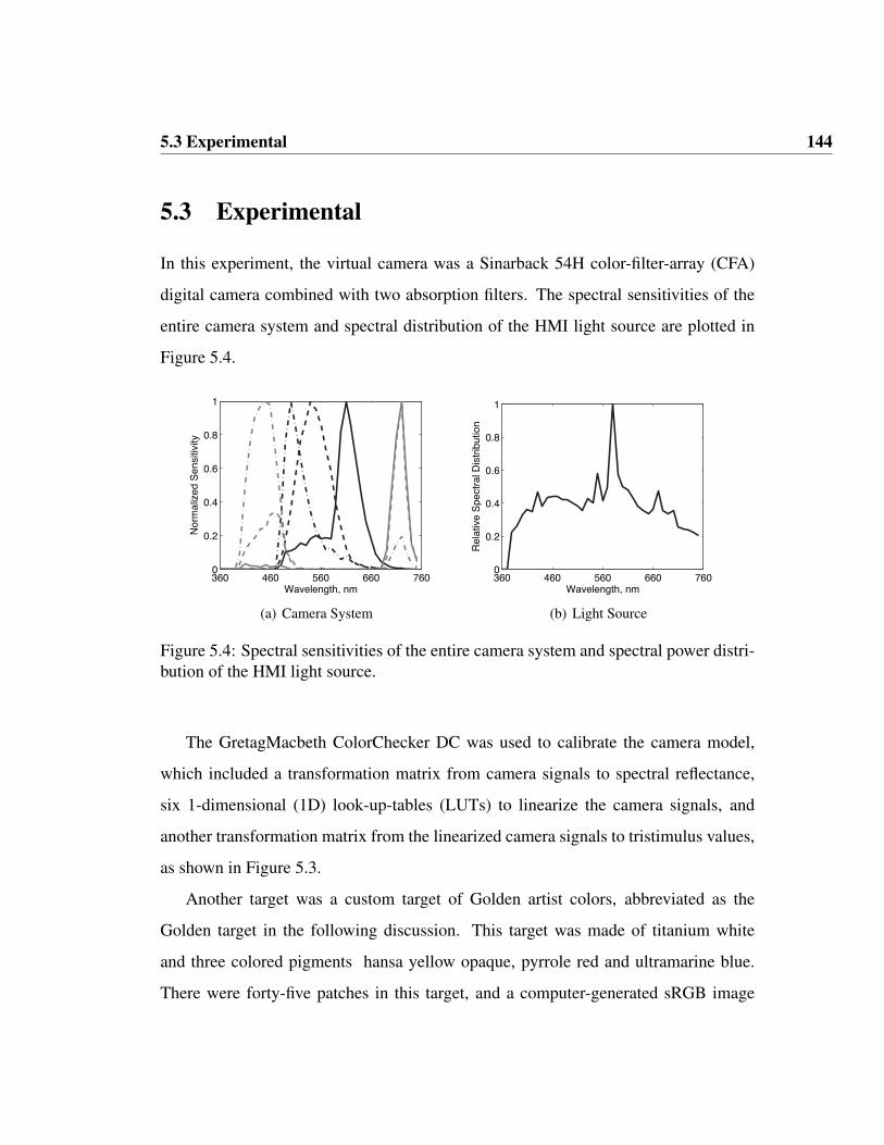
5.3 Experimental 144
5.3 Experimental
In this experiment, the virtual camera was a Sinarback 54H color-filter-array (CFA)
digital camera combined with two absorption filters. The spectral sensitivities of the
entire camera system and spectral distribution of the HMI light source are plotted in
Figure 5.4.
360 460 560 660 7600
0.2
0.4
0.6
0.8
1
Wavelength, nm
Nor
mal
ized
Sen
sitiv
ity
(a) Camera System
360 460 560 660 7600
0.2
0.4
0.6
0.8
1
Wavelength, nm
Rel
ativ
e S
pect
ral D
istr
ibut
ion
(b) Light Source
Figure 5.4: Spectral sensitivities of the entire camera system and spectral power distri-bution of the HMI light source.
The GretagMacbeth ColorChecker DC was used to calibrate the camera model,
which included a transformation matrix from camera signals to spectral reflectance,
six 1-dimensional (1D) look-up-tables (LUTs) to linearize the camera signals, and
another transformation matrix from the linearized camera signals to tristimulus values,
as shown in Figure 5.3.
Another target was a custom target of Golden artist colors, abbreviated as the
Golden target in the following discussion. This target was made of titanium white
and three colored pigments hansa yellow opaque, pyrrole red and ultramarine blue.
There were forty-five patches in this target, and a computer-generated sRGB image

5.4 Results and Discussions 145
of this target was shown in Figure 5.5. All these samples were carefully prepared
and measured using a GretagMacbeth ColorEye XTH sphere spectrophotometer with
specular component included.
Figure 5.5: Computer-generated sRGB image of the Golden Target.
5.4 Results and Discussions
5.4.1 Original Matrix R Method
In this section, both the spectral and colorimetric accuracies of the matrix R method
are provided in detail. The colorimetric error metrics include color difference CIELAB
and CIEDE2000 under CIE illuminant D65 and for the 2-degree observer, while the
spectral error metrics include spectral RMS error and two metamerism indices that
consist of both a parameric correction for CIE illuminant D65 (A) and color difference
CIEDE2000 under CIE illuminant A (D65).
Statistical results of the colorimetric and spectral error metrics for the calibration
and the custom targets were listed in Tables 5.1 and 5.2. It can be seen that the col-

5.4 Results and Discussions 146
orimetric performances for both targets were very good. It means that the nonlinear
optimization used to minimize color difference was an effective technique to improve
colorimetric performance. However, the spectral accuracy was unsatisfactory. For
example, the mean spectral RMS error for the Golden target was 3.84%, and the max-
imum metamerism index for the ColorChecker DC was very high. Measured and pre-
dicted spectral reflectance factors using the original matrix R method for two patches in
the Golden target were plotted in Figure 5.6. The method had some degree of difficulty
in matching the long wavelength reflectance tail of the ultramarine blue (bottom).
Table 5.1: Colorimetric and spectral accuracies for calibration target - GretagMac-beth ColorChecker DC (CCDC) between measured and predicted spectral reflectancefactors.
Statistics ∆Eab ∆E00 RMS (%) MI (D65 → A) MI (A → D65)Mean 1.06 0.69 1.48 0.24 0.30
Std. Dev. 0.82 0.43 0.81 0.63 0.7090% percentile 2.29 1.36 2.30 0.38 0.51
Min 0.07 0.07 0.08 0.01 0.01Max 4.31 2.42 4.83 9.34 10.17
Table 5.2: Colorimetric and spectral accuracies for the custom Golden target betweenmeasured and predicted spectral reflectance factors without pigment mapping.
Statistics ∆Eab ∆E00 RMS (%) MI (D65 → A) MI (A → D65)Mean 1.86 1.02 3.84 0.91 1.09
Std. Dev. 1.34 0.64 1.34 0.74 0.8590% percentile 3.97 2.01 5.61 2.09 2.68
Min 0.17 0.14 1.49 0.08 0.07Max 5.28 2.64 6.02 2.92 3.49

5.4 Results and Discussions 147
5.4.2 Improved Matrix R Method
The original matrix R method was improved by incorporating pigment mapping. The
predicted spectral reflectance factor by the original matrix R method from the six-
channel camera signals was used to estimate the concentrations of pigments for each
patch, which in turn was used to reconstruct spectral reflectance factor. This approach,
as indicated by the statistical results in Table 5.3, did not change colorimetric perfor-
mance, but as expected, significantly improved spectral accuracy. The mean RMS error
decreased from 3.8% to 1.1%, and the maximum RMS error was reduced by almost
two fold. The two metameric indices also decreased appreciably.
Table 5.3: Colorimetric and spectral accuracies for the custom Golden target betweenmeasured and predicted spectral reflectance factors with pigment mapping.
Statistics ∆Eab ∆E00 RMS (%) MI (D65 → A) MI (A → D65)Mean 1.86 1.02 1.05 0.25 0.36
Std. Dev. 1.34 0.64 0.48 0.22 0.2690% percentile 3.97 2.01 1.66 0.47 0.64
Min 0.17 0.14 0.27 0.00 0.01Max 5.28 2.64 2.35 0.83 1.13
Figure 5.6 illustrates the improvement of spectral accuracy by pigment mapping
for two selected patches of the Golden target. For the white patch, the predicted re-
flectance by the improved matrix R method almost overlapped with the measurement.
The improvement was even more pronounced for the ultramarine blue, where the pre-
dicted reflectance with pigment mapping followed much more closely with the mea-
surement. It is obvious that pigment mapping improved the spectral accuracy of the
original matrix R method.

5.5 Conclusions 148
360 460 560 660 7600
0.2
0.4
0.6
0.8
1
Wavelength, nm
Ref
lect
ance
Fac
tor
Patch No. 1
Measurement
W/O Pigment Mapping
W Pigment Mapping
(a) White Patch
360 460 560 660 7600
0.1
0.2
0.3
0.4
0.5
0.6
0.7
0.8
Wavelength, nm
Ref
lect
ance
Fac
tor
Patch No. 15
Measurement
W/O Pigment Mapping
W Pigment Mapping
(b) Blue Patch
Figure 5.6: Spectral accuracy of the six-channel virtual camera without pigment map-ping (dashed line) and with pigment mapping (dash dotted line) compared with in situspectrophotometry (solid line) for two patches of the Golden target.
5.5 Conclusions
Compared with conventional color imaging, spectral imaging takes advantage of much
more embedded information in spectral reflectance. The original matrix R method
combined the benefits of both spectral and colorimetric imaging, and provided a highly
accurate match to an original target, both spectrally and colorimetrically. The spectral
accuracy of the matrix R method was further improved by pigment mapping. A virtual
camera model was simulated and used along with a custom target of Golden artist
colors to verify the recovery of the smoothness of spectral reflectance predicted by the
original matrix R method. Incorporating pigment mapping reduced the mean spectral
RMS error for the custom target from 3.8% to 1.1% and the maximal RMS by almost
two fold. It also decreased the degree of metamerism appreciably. In conclusion,
by incorporating pigment mapping, the improved matrix R method can achieve even
higher spectral accuracy.

Chapter 6
Color-Match Prediction for
Translucent Paints
6.1 Introduction
The use of Kubelka-Munk (K-M) turbid media theory (Kubelka and Munk, 1931;
Kubelka, 1948; Kubelka, 1954) for predicting the spectral reflectance factor of opaque
specimens from their constituent optical properties is well established in practice and
well described in the literature (Allen, 1966; Allen, 1974; Allen, 1980; Nobbs, 1997;
Judd and Wyszecki, 1975; Berns, 2000). Practical success has been achieved by the
reduction in mathematical complexity when a specimen is opaque, the elimination of
controlling thickness, and extensive experimentation for a variety of materials. Its
use in predicting translucent specimens has been much more limited. Davidson and
Hemmendinger (Davidson and Hemmendinger, 1966) introduced a method to deter-
mine paint optical constants, and then tested the validity of these constants for only
opaque mixtures. Nobbs (Nobbs, 1997) discussed colorimetric match prediction of

6.1 Introduction 150
lithographic inks using a partial derivative approach. The Ph.D. dissertation of Hoffen-
berg (Hoffenberg, 1972) is by far the most comprehensive publication that considered
the determination of the optical constants of 13 basic lithographic printing inks and an
automated procedure for spectral-match prediction of ink mixtures.
Our interests in K-M theory are the applications of color science to art conservation
science and spectral-based imaging, archiving, and reproduction of artwork. This has
included pigment selection for developing a prototype calibration target for spectral
imaging (Mohammadi et al., 2004a; Mohammadi et al., 2005), pigment identification
based upon spectral estimation (Berns and Imai, 2001), image segmentation and pig-
ment mapping of paintings (Zhao et al., 2006), improving spectral imaging by incorpo-
rating pigment mapping (Zhao et al., 2005a), digitally rejuvenating the appearance of
paintings having temporal color changes (Berns, 2005b; Berns et al., 2006), and pig-
ment selection for restorative inpainting (Berns et al., 2002; Berns and Mohammadi,
2007a).
Thus far, we have limited our experimentation to opaque paint samples and when
evaluating paintings, assumed that the paint layer was opaque when unvarnished, or
if varnished, that the varnish layer was transparent. For many paintings, the paint
layer may be composed of multiple layers of various thicknesses and opacities, rang-
ing from transparent glazes to an opaque ground. In these cases, film thickness should
be known for each layer and the constituents’ optical constants are defined as a func-
tion of thickness. If each layer has a different refractive index, this should also be
considered. K-M theory can be used to model the optical behavior treating each layer
as a separate homogeneous layer in optical contact with adjacent layers. However, the
two-flux assumption of K-M theory may not model such a multiple scattering system
with sufficient accuracy, particularly as the scattering becomes heterogeneous. In these

6.1 Introduction 151
cases, the many-flux theory would be used to characterize the paints optical constants
and to predict spectral reflectance factor of translucent films and other complex multi-
layer systems (Mudget and Richard, 1971; Billmeyer et al., 1980; Mehta and Shah,
1987; Joshi et al., 2001). Unfortunately, comprehensive experiments have not been de-
scribed in predicting the spectral reflectance factor of translucent paint films comparing
many-flux and K-M theories. Modern implementation of the many-flux theory tends
to be proprietary. Because K-M theory is familiar within the art conservation science
field and well models the optical properties of artist paints (Berns et al., 2002; Berns
and Mohammadi, 2007a), we were interested in testing its applicability to translucent
artist paints and glazes. Thus, this chapter reviews published methods to characterize
translucent paint films and tests these methods in comparison to the opaque K-M ap-
proach for artist acrylic paints and glazes.
In our specific case, we were interested in determining the absolute optical prop-
erties of paints and predicting the spectral reflectance factors of both translucent and
opaque paint mixtures. Golden matte fluid acrylic paints and glazes were used in this
research. These paints were selected to encompass a variety of opacities along with a
wide range of reflectance factors. The four glazes were included to ensure materials
that were transparent, or nearly so. Two different whites were also used, each with
quite different refractive indices, and as a consequence, different opacities: titanium
dioxide white and zinc white. Paints films were made using a BYK-Gardner applicator
bar having an opening of 6 mils on Leneta opacity chart Form 3B with both a white
and a black background for opacity evaluation. Concentration was defined as fraction
of the total weight, based on wet paint. The scale used was an Acculab VI-200 with a
readability of 0.01g. Spectral reflectance factor was measured using a ColorEye XTH
integrating sphere spectrophotometer with specular component excluded. Three mea-
6.2 Database Development 152
surements on different spots over each background of the opacity chart were taken and
then averaged. For each paint, two samples a masstone and a mixture with zinc white
(tint) were prepared to determinate both absorption and scattering coefficients. Zinc
white was used since it was less opaque than titanium dioxide white, and tints with zinc
white were more transparent. In order to test the accuracy of the paint constants, some
test samples were also prepared. Eighteen samples were prepared with one chromatic
paint and white paint (either zinc white or titanium dioxide white). Fifty-three sam-
ples were prepared with two chromatic paints with a relative ratio of 1:1, and another
53 samples were made up of two chromatic paints with either zinc white or titanium
dioxide white, with a relative ratio of 1:1:2. All those test samples were prepared in
the same way on the same opacity chart as the calibration samples.
6.2 Database Development
6.2.1 Methods for Determining Optical Constants
The pigment optical constants – absorption and scattering coefficients – in the K-M
equations can be determined either on an absolute basis or relative to white with an as-
sumed scattering coefficient of unity (Allen, 1980). The relative method is acceptable
when the samples are prepared at full opacity, while the absolute method is required
for translucent samples (Davidson and Hemmendinger, 1966).
There are four distinct methods to determine the absolute values of absorption and
scattering coefficients of each pigment. Before the discussion of the detailed mathe-
matical derivations and methodologies for these methods, it is useful to give a brief
overview of K-M theory.
The general mathematical form of K-M theory is expressed as Eq. (6.1) in which

6.2 Database Development 153
the reflectance factor of a film can be calculated from the absorption K and scattering
S coefficients of the film, the reflectance factor of the background Rg, the film thick-
ness X , and two auxiliary variables a and b. The symbol coth x means hyperbolic
cotangent function. (These constants are all functions of wavelength; for clarity, this is
omitted.)
R =1−Rg [a− b coth (bSX)]
a−Rg + b coth (bSX)(6.1)
Equation (6.1) can be simplified for opaque specimens assuming that the film thick-
ness approaches infinity (X → ∞). Infinite thickness means that reflectance factor,
referred as reflectivity R∞, will no longer change as the film thickness further in-
creases. Reflectivity R∞ can be calculated from the ratio between the absorption and
scattering coefficient K/S with Eq. (6.2), and vise versa using Eq. (6.3).
R∞ = a− b = 1 + K/S −√
(K/S)2 + 2 (K/S) (6.2)
K
S=
(1−R∞)2
2R∞(6.3)
Next, it is necessary to build the relationship between a mixture paint sample and
its constituents. For this chapter, only paints, either in tube or jar form, were consid-
ered; that is, the paint medium, pigment(s) and any additives were not characterized
individually, but as a single material, paint. Under the assumption of additivity and
scalability (Duncan, 1949), both the absorption and scattering coefficients for the mix-
ture can be easily calculated from the coefficients of its component paints, weighted
by the corresponding concentrations ci, commonly referred to as two-constant K-M
theory. The small case k and s are the absorption and scattering coefficients at unit

6.2 Database Development 154
concentration.
K =m∑
i=1
ciki (6.4)
S =m∑
i=1
cisi (6.5)
Finally, the discontinuity of refractive indices between the air and paint film is
not considered in K-M theory and is accounted for using the so-called Saunderson
equations (Saunderson, 1942) relating the measured reflectance factor to the internal
reflectance factor, described in Eqs. (6.6) and (6.7), where Rmeas represents the re-
flectance factor measured with an integrating sphere spectrophotometer with specular
component excluded, R is the internal reflectance factor, r1 is the fraction of reflected
light from the air-film interface, and r2 describes the fraction of reflected diffuse light
incident on the underside of the film layer.
Rmeas =(1− r1) (1− r2) R
1− r2R(6.6)
R =Rmeas
(1− r1) (1− r2) + r2Rmeas
(6.7)
6.2.1.1 Black-White Method
This method has been well discussed in the literature (Allen, 1980; Nobbs, 1997;
Judd and Wyszecki, 1975; Davidson and Hemmendinger, 1966; Hoffenberg, 1972;
Volz, 2001) and requires just one paint sample of the same thickness over a white
and over a black background, which was referred to simply as the black-white method
by Hoffenberg (Hoffenberg, 1972). For each pair of the background and film over
this background, their reflectance factors are measured. Two pairs of the reflectance

6.2 Database Development 155
data (Rw, Rgw) or (Rk, Rgk) are input into the general hyperbolic form of K-M theory,
where the subscript g stand for background, and the subscripts w and k represent white
and black, respectively. Then the absorption and scattering coefficients can be solved
simultaneously based on these two equations.
The mathematical derivation starts from the hyperbolic form of K-M theory. Equa-
tion (6.1) can be rearranged as
coth (bSX) =(1 + RRg)− a (R + Rg)
b (R−Rg)(6.8)
The auxiliary variable a can be solved by substituting data (Rw, Rgw) and (Rk, Rgk)
into Eq. (6.8) and equating the right-hand side of Eq. (6.8). After some algebra,
a =(Rw −Rk)(1 + RgwRgk)− (Rgw −Rgk)(1 + RwRk)
2(RwRgk −RkRgw)(6.9)
Next, the scattering and absorption coefficients can be determined by substitut-
ing either pair of reflectance factors, e.g., (Rk, Rgk) into Eq. (6.8). With the help of
the trigonometric function coth (x− y) = 1−coth (x) coth (y)coth (x)−coth (y)
, the scattering coefficient
including thickness can be expressed as shown in Eq. (6.10), where coth−1(x) repre-
sents the inverse hyperbolic cotangent function.
SX =1
b
[coth−1
(a−Rk
b
)− coth−1
(a−Rgk
b
)](6.10)
Finally, the absorption coefficient is calculated from the scattering coefficient via
the auxiliary variable [Eq. (6.11)]. Since the pigment mass per unit area is determined
by both the film thickness and the pigment concentration, it is necessary to compensate
for film thickness in order to accurately predict the colorant formulation. Typically,
film thickness X is held constant and defined as unity for all the samples. SX can be

6.2 Database Development 156
simply referred to as the scattering coefficient in the following discussion, as is KX .
KX = SX (a− 1) (6.11)
For an ideal black backing with Rgk = 0, Eq. (6.8) can be further simplified.
SX =1
bcoth−1
(1− aRk
bRk
)(6.12)
Either (Rw, Rgw) or (Rk, Rgk) can be substituted into Eq. (6.10) for determining
the scattering coefficient SX . It is better to take the pair that gives the smaller error
in SX . The error calculation is done using differential coefficients to determine how a
small change in measured reflectance factor produces a corresponding change in SX .
The detailed analysis can found in (Volz, 2001). The output SX is calculated based on
the pair with the smaller error in SX . The derived equations (6.10) and (6.12) for de-
termining the scattering coefficient were verified in the reference (Judd and Wyszecki,
1975). In this case, the pigment constants can be calculated directly from two pairs of
reflectance data (Rw, Rgw) and (Rk, Rgk).
Another approach is to use a nonlinear iterative algorithm, discussed by (Allen,
1980) and (Hoffenberg, 1972). Although the pigment constants have physical mean-
ing, their numerical solutions might be negative or complex, possibly caused by im-
precision reflectance measurement or too large a film thickness. Numerical examples
are provided later.
6.2.1.2 Infinite Method
This method has been discussed by (Allen, 1980; Volz, 2001; Cairns et al., 1976).
It requires a paint sample at infinite optical thickness and another translucent sample

6.2 Database Development 157
with known thickness over a background. Both samples contained the same 100%
pure paint only at different film thickness. The method is referred as the classical
method by (Volz, 2001), but called as the infinite method in the following discussion
because a paint sample at infinite optical thickness is required. Reflectivity R∞ can be
obtained from the paint sample with infinite thickness. The auxiliary valuable a can be
expressed as Eq. (6.13) by adding unity on both sides of Eq. (6.3), and b can also be
derived from Eqs. (6.2) and (6.13).
a =1
2
(1
R∞+ R∞
)(6.13)
b =1
2
(1
R∞−R∞
)(6.14)
For the previous black-white method, the auxiliary valuable a is calculated from
two pairs of reflectance factors (Rw, Rgw) and (Rk, Rgk) [Eq. (6.9)], while in this
method, this variable is obtained from reflectivity R∞ [Eq. (6.13)]. For the infinite
method, since the auxiliary variable a is calculated based on only one measurement
instead of four measured reflectance factors, measurement uncertainty has less of an
effect on the accuracy of the pigment constants (Volz, 2001). When an opaque film is
available, the infinite method should be adopted. After that, the pigment constants can
be calculated using Eqs. (6.10) and (6.11) with the reflectance factors (R,Rg) of both
another translucent sample over the background and the background.
References (Allen, 1980; Cairns et al., 1976) provided another formula, Eq. (6.15),
to calculate the scattering coefficient from the reflectivity R∞ and a pair of reflectance
factors (R,Rg) of both the film over the background and the background. The symbol
ln (x) means the natural logarithm function. The formula originally comes from the
article in German published by (Kubelka and Munk, 1931) in 1931 and its derivation

6.2 Database Development 158
begins from the two differential equations of K-M theory. For completeness and a bet-
ter understanding of K-M theory, the detailed mathematical derivation of this formula
can be found in Appendix B.4. It can also be shown that Eq. (6.15) is equivalent to Eq.
(6.10) if the auxiliary variables are calculated from the reflectivity R∞ [Eqs. (6.13)
and (6.14]. The proof is also shown in Appendix B.4.
SX =R∞
1−R2∞
ln
[(1−RR∞) (R∞ −Rg)
(1−RgR∞) (R∞ −R)
](6.15)
6.2.1.3 Masstone-Tint Method
This method is a simplified version of the tint ladder method (Cairns et al., 1976), an
over-determined method where about five to eight tints are prepared at various ratios
of chromatic paint with white paint along with a pure chromatic paint, called the mas-
stone. Using linear or nonlinear optimization, this set of samples are used to estimate
the optical constants for a paint of interest. Given that the optical properties of the white
paint are pre-calculated, a minimum of two samples is required. For the opaque case
the optical constants can be solved by two linked equations, while for the translucent
case a nonlinear iterative algorithm is required to find the constants. Previous research
has found that a masstone and a tint in the neighborhood of maximum chroma yielded
to the best performance (Mohammadi and Berns, 2004; Zhao and Berns, 2006).
For the opaque case, the ratio between absorption and scattering coefficients K/S
can be directly calculated from the corresponding reflectance factors for both the mas-
stone and tint samples using Eq. (6.3). For the tint sample, the ratio K/S can be
further expressed as the summation of unit absorption coefficients of its component
paints [Eq. (6.4)] divided by summation of unit scattering coefficients [Eq. (6.5)]. It is
worth noting that lower case k and s are the same as upper case K and S, but reserved

6.2 Database Development 159
for the masstone sample. The subscript w specifies the white paint.
(K
S
)masstone
=k
s(6.16)
(K
S
)tint
=ck + (1− c)kw
cs + (1− c)sw
(6.17)
After that, the unit absorption and scattering coefficients for the paint of interest
can be calculated from(
KS
)masstone
,(
KS
)tint
and the paint concentration c of the tint.
s =1− c
c
(KS
)masstone
sw − kw(KS
)masstone
−(
KS
)tint
(6.18)
k = s
(K
S
)masstone
(6.19)
For the translucent case, since the ratio K/S cannot be expressed as a function of
reflectance factor, a constrained nonlinear iterative algorithm is required to solve the
absorption and scattering coefficients. The absorption and scattering coefficients for
the tint can be expressed as following under the assumption of additivity and scalability
(Duncan, 1949). Equation (6.1) is used to predict reflectance factor from these coef-
ficients for both the tint and masstone samples. The objective function is to minimize
the average spectral root-mean-square (RMS) error between measured and predicted
reflectance factors for these two samples by adjusting k and s of the pigment to be
characterized. Both k and s are constrained to be no less than zero.
K = ck + (1− c)kw (6.20)
S = cs + (1− c)sw (6.21)

6.2 Database Development 160
There are several issues associated with using constrained nonlinear iterative algo-
rithms. Since both k and s are wavelength dependent, the number of variables to be
optimized is two times the number of the wavelengths. Two paint samples – masstone
and tint – can form the same number of equations as the number of variables to be opti-
mized, or twice as many as the number of variables if the reflectance factors over both
backgrounds for both samples are considered. The running time increases dramatically
with the increase in the number of variables requiring optimization. The solution might
be a local minimum and sensitive to the choice of starting value. Most importantly, the
algorithm might not be able to find a feasible local minimum satisfying the constraint.
6.2.1.4 Two-Region Method
Few paint films are totally opaque or totally translucent across the entire visible spec-
trum. Rather, these paint films are partially opaque and partially translucent, hence
the name, two-region method. Within the region of strong absorption, where the film
is opaque, the masstone-tint method for the opaque case is used while outside the re-
gion of absorption, where the film is translucent, one of the three methods described
above for the translucent case is used. Occasionally it is difficult or impossible to
make a completely opaque film and for these cases, the infinite method does not work
and the black-white method is adopted to determine the pigment constants within the
translucent region. The constrained nonlinear iterative algorithm is not recommended
because of the limitations discussed above.
The two-region method was originally proposed by (Davidson and Hemmendinger,
1966) for paint films and by (Hoffenberg, 1972) for printing inks. In the Davidson and
Hemmendinger approach, within the region of absorption, the masstone-tint method
for the opaque case was used, while outside region of absorption, either the masstone-

6.2 Database Development 161
tint method for the translucent case or the black-white method was used. Unfortu-
nately, they did not discuss explicitly how to choose the method for the translucent
region and how to delimit the spectrum into the two wavelength regions. In the Hof-
fenberg approach, both the black-white and masstone-tint methods were used to char-
acterize the optical properties of the basic inks. At each wavelength, an error index for
both methods was calculated, and the method that achieved the smallest error was used
to determine each constant. The error index for both methods was the absolute value of
the difference between the measured reflectance of the masstone over the black and the
value calculated using these constants obtained from these methods. The error index
is unnecessary if the entire wavelength range is separated into two parts in advance. In
the current research, several features were added including a determination of opacity
or translucency and smoothing between the two regions. The details are described be-
low.
The first step was to determine opacity. TAPPI (Technical Association of the Pulp
and Paper Industry) opacity, C0.89, was defined originally as the ratio between re-
flectance of layer with ideal black background (Rgk = 0) and reflectance of layer
with white background (Rgw = 0.89) (Judd and Wyszecki, 1975). In this research,
in similar fashion to TAPPI opacity, the opacity O was defined as the ratio between
reflectance factors over a black and over a white background for the masstone sample.
O =Rk
Rw
(6.22)
Ideally, O defines complete opacity. Because of measurement uncertainty, this value
was too restrictive and the critical value of 0.98 was used. Wavelengths when O > 0.98
were considered opaque, otherwise translucent. This reasonable value was chosen to
minimize the number of the pivot points connecting opaque and translucent regions.

6.2 Database Development 162
An example of phthalocyanine green is given. The measured reflectance factors for
the masstone sample of phthalocyanine green over the white and black backgrounds
are plotted in Fig. 6.1(a), and the opacity is plotted in Fig. 6.1(b). If the critical value
was set to 0.98, there were two pivot points (490 and 530 nm), while five pivot points
for the critical value of 0.99 (400, 480, 540, 620 and 630 nm). Too many pivot points
make smoothing these transition regions harder, and more smoothing operations would
introduce extra error. So the critical value of 0.98 was chosen.
(a) (b)
Figure 6.1: (a) Measured reflectance factors of phthalocyanine green masstone sampleover both a white (solid line) and a black (dashed line) background of an opacity chart.(b) The ratio of measured reflectance factors of phthalocyanine green masstone samplebetween over the black and over the white backgrounds (solid line). The dashed anddash-dotted lines indicate the critical value of 0.99 and 0.98, respectively.
In the opaque region, the measured reflectance factors over both black and white
backgrounds were averaged. Following the Saunderson correction, the ratio K/S for
both masstone and mixture samples were calculated from Eq. (6.3). The absorption
and scattering coefficients for the pigment were estimated using Eqs. (6.18) and (6.19).
In the translucent region, the measured reflectance factors over both black and

6.2 Database Development 163
white backgrounds for the masstone sample were used to characterize the pigment con-
stants. After the Saunderson correction, the absorption and scattering coefficients were
calculated from Eqs. (6.9)-(6.11) using the two pair of reflectance factors (Rw, Rgw)
and (Rk, Rgk).
Typically, these two regions often are not connected smoothly. Since it is known
that the spectral curves of the paint’s constants should be smooth, special care should
be considered in the connection region. The smoothing operation can reduce the un-
evenness but might introduce error in the paints constants and can cause some fine
spectral feature loss. The wavelength interval is 10 nm for most commercial spec-
trophotometers; the tiny peak of cobalt blue around 490 nm will disappear if a smooth-
ing filter is used carelessly. The scattering coefficients of cobalt blue with different
smoothing strategies are plotted in Fig. 6.2(a), and the predicted reflectance factors
with these coefficients are plotted in Fig. 6.2(b). Due to the lower sampling rate of
measured reflectance factor, the first smoothing strategy was to smooth only the pivot
point(s) connecting the opaque and translucent regions based on the second-order poly-
nomial fitting on four neighborhood points surrounding each pivot point. The second
and third strategies were to smooth the whole spectrum using the simple average filter
with window size of three and five, respectively. For cobalt blue, the two pivot points
were 540 nm and 650 nm, and the opaque region located between these two points. For
the first strategy, the scattering spectrum was connected smoothly after its coefficients
at these two points were modified, as shown in Fig. 6.2(a). The error introduced by the
modification of only the pivot point was negligible. For the second and third strategies,
the scattering spectrum was appreciably smoother as the window size increased from
three to five points. However, the predicted reflectance factors deviated considerably
from the measurements, and the tiny peak around 490 nm vanished. So only the pivot

6.2 Database Development 164
point(s) connecting the opaque and translucent regions was smoothed and modified.
For most paints, one pivot point existed, while for a few paints, there were two points.
(a) (b)
Figure 6.2: (a) The scattering coefficients of cobalt blue based on the two-regionmethod without smoothing (solid line) and with three smoothing strategies. The firststrategy is to smooth only the pivot points (540 nm and 650 nm) connecting opaqueand translucent regions (dashed line). The second and third strategies are to smooththe entire spectrum using an average filter with window size of three (dash-dotted line)or five (dotted line), respectively. (b) Measured (solid line) and predicted spectralreflectance factors of cobalt blue masstone sample over both backgrounds using theabsorption and scattering coefficients calculated from the three smoothing strategies.
Here is the summary of this method. Calculations were performed at each wave-
length. The input values included the pigment constants for the white paint, the mea-
sured reflectance factors for both white and black backgrounds of the contrast paper,
and the masstone and tint samples over both backgrounds. The pigment constants for
the white paint were calculated using the black-white method in advance. All the re-
flectance factors were corrected using the Saunderson equation [Eq. (6.7)]. Then the
opacity was calculated. If the opacity was greater than the critical value of 0.98, the
pigment constants were calculated for the opaque region using Eqs. (6.3), (6.18) and
(6.19). If not, the pigment constants were calculated for the translucent region using

6.2 Database Development 165
Eqs. (6.9)-(6.11). Finally, the pivot point(s) between the opaque and translucent re-
gions was smoothed using the second-order polynomial fitting on the four neighboring
points surrounding each pivot point.
6.2.2 Problems with Numerical Solutions
The pigment constants - absorption and scattering coefficients - have physical mean-
ing and should be greater than or equal to zero. However, numerical solutions can
sometimes lead to either negative or complex numbers.
Here is a numerical example of determining the absorption and scattering coeffi-
cients for zinc white. Reflectance data have been corrected by the Saunderson equation
[Eq. (6.7)]. The auxiliary variable a, the absorption k and scattering s coefficients were
calculated using Eqs. (6.9)-(6.11), and listed in Table 6.1 for four wavelengths. The a
values were less than unity at 440 nm and 450 nm, so the corresponding b values were
complex numbers since b =√
(a2 − 1). The value of a was calculated using Eq. (6.9)
from four reflectance factors, so uncertainty from all four reflectance measurements
contributes to the uncertainty of a. Alternatively, a can also be calculated from reflec-
tivity using the infinite method, and its precision can be improved since it requires just
one measurement (Volz, 2001). However, it is sometimes difficult to apply the paint
at full opacity. One solution to avoid complex values is to clip the absorption k to a
predefined minimum value, as was done in this evaluation.
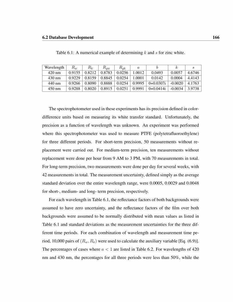
6.2 Database Development 166
Table 6.1: A numerical example of determining k and s for zinc white.
Wavelength Rw Rk Rgw Rgk a b k s
420 nm 0.9155 0.8212 0.8783 0.0256 1.0012 0.0493 0.0057 4.6746430 nm 0.9229 0.8159 0.8845 0.0254 1.0001 0.0142 0.0004 4.4143440 nm 0.9266 0.8090 0.8888 0.0254 0.9995 0+0.0307i -0.0020 4.1763450 nm 0.9288 0.8020 0.8915 0.0251 0.9991 0+0.0414i -0.0034 3.9738
The spectrophotometer used in these experiments has its precision defined in color-
difference units based on measuring its white transfer standard. Unfortunately, the
precision as a function of wavelength was unknown. An experiment was performed
where this spectrophotometer was used to measure PTFE (polytetrafluoroethylene)
for three different periods. For short-term precision, 50 measurements without re-
placement were carried out. For medium-term precision, ten measurements without
replacement were done per hour from 9 AM to 3 PM, with 70 measurements in total.
For long-term precision, two measurements were done per day for several weeks, with
42 measurements in total. The measurement uncertainty, defined simply as the average
standard deviation over the entire wavelength range, were 0.0005, 0.0029 and 0.0048
for short-, medium- and long- term precision, respectively.
For each wavelength in Table 6.1, the reflectance factors of both backgrounds were
assumed to have zero uncertainty, and the reflectance factors of the film over both
backgrounds were assumed to be normally distributed with mean values as listed in
Table 6.1 and standard deviations as the measurement uncertainties for the three dif-
ferent time periods. For each combination of wavelength and measurement time pe-
riod, 10,000 pairs of (Rw, Rk) were used to calculate the auxiliary variable [Eq. (6.9)].
The percentages of cases where a < 1 are listed in Table 6.2. For wavelengths of 420
nm and 430 nm, the percentages for all three periods were less than 50%, while the

6.2 Database Development 167
percentages were above 50% for wavelengths of 440 nm and 450 nm. These results
are consistent with Table 6.1. For short-term precision, the percentages at each of the
four wavelengths were considerably different; at 420 nm and 430 nm, the probabilities
of a < 1 were low while for 440 nm and 450 nm, the probabilities were much higher.
The uncertainty increased as the time period increased. It is clear that measurement
uncertainty contributed to unrealistic values.
Table 6.2: The percentage of cases where a < 1 for each listed time period.
Wavelength Short Term Medium Term Long Term420 nm 0.0 1.4 11.4430 nm 18.2 38.3 46.9440 nm 100.0 76.5 72.5450 nm 100.0 96.5 78.8
Determining absorption and scattering coefficients for titanium dioxide white is the
second example, listed in Table 6.3. The auxiliary values a were all greater than one.
The absorption and scattering coefficients were complex numbers at 370 nm. It was
caused by the inverse hyperbolic cotangent function coth−1(x), which returns a real
number only when |x| > 1. One possible reason for this occurrence is the measurement
uncertainty shown above. It is suspicious that the reflectance values over the white
background were not greater than those over the black background from 360 nm to 380
nm. A similar analysis as above was performed for the three different time periods. The
percentages of cases where the scattering coefficients were complex numbers are listed
in Table 6.4. This table is quite different from Table 6.2. The percentages are close
to 50% for all three wavelengths (from 360 nm to 380 nm) and for all three periods.
This implies that cases where s is a complex number is independent of measurement
uncertainty. Another reason is that the paint mass per unit area was too large (Volz,

6.2 Database Development 168
2001), that is to say, the film was not sufficiently thin when the paint concentration was
fixed. Because titanium dioxide white is both a strong absorber and scatterer at short
wavelengths, the paint film was not sufficiently translucent. Because k and s values
at these short wavelengths have low credibility, these wavelengths are skipped. The
calculation of k and s for all the paints were carried out in the general visible range
between 400 nm and 700 nm.
Table 6.3: A numerical example of determining k and s for titanium dioxide white.
Wavelength Rw Rk Rgw Rgk a b k s360 nm 0.1645 0.1645 0.3734 0.0256 3.1223 2.9579 13.1800 6.2100370 nm 0.1990 0.1992 0.6298 0.0266 2.6098 2.4106 2.69+1.05i 1.67+0.65i380 nm 0.2684 0.2684 0.7936 0.0269 1.9974 1.7291 10.3960 10.4230390 nm 0.4282 0.4278 0.8484 0.0266 1.3823 0.9544 1.5263 3.9923
Table 6.4: The percentage of cases where s was a complex number for each listed timeperiod.
Wavelength Short Term Medium Term Long Term360 nm 50.4 50.5 50.4370 nm 61.2 52.3 51.8380 nm 50.4 50.4 50.4390 nm 33.7 45.8 47.0
6.2.3 Determination of Optical Constants for White Paints
Instrumental-based color-match prediction requires three steps. The first and most im-
portant step is to characterize the optical properties of each component forming the
database, in this case each paint. The second step is to select the set of paints that
match the standard according to user-defined criteria such as spectral similarity, color
6.2 Database Development 169
differences under one or more illuminants, metamerism, and cost. The final step is to
calculate the recipe. The success of any color-match prediction relies on how well the
first step is executed, that is, how well the paints have been prepared and calibrated.
The characterization of the optical constants will be first discussed, and then these
constants will be applied in color-match prediction. The fraction r1 in Saunderson
Equation was set to 0.03. The other fraction r2 was set to 0.6, the theoretical value for
a refractive index of 1.5 for the paint film and collimated flux at normal incidence. See
reference (Berns and de la Rie, 2003) to determine these constants for other combina-
tions of angle and refractive index. The refractive-index-corrected reflectance factors
were input into the general form of K-M theory [Eq. (6.1)].
There were two white paints – zinc white and titanium dioxide white. The re-
flectance factors of zinc white over both backgrounds are plotted in Figure 6.3(a). The
spectral reflectance factor of zinc white over the white background was considerably
higher than that over the black background above 400 nm. The spectra of zinc white
over the white and over the black backgrounds diverged increasingly with wavelength.
The large divergence between these two spectra indicates that the zinc white film had
low opacity and inadequately hid the background. The reflectance factors of titanium
dioxide white are also plotted in Figure 6.4(a). Compared with zinc white, titanium
dioxide white was more opaque since the difference between two spectral curves was
less pronounced. These two white paints were characterized using the black-white
method. The absorption and scattering coefficients for zinc white and titanium dioxide
white are also plotted in Figures. 6.3(b) and 6.4(b), respectively. The scattering coeffi-
cient of titanium dioxide white was significantly larger than that of zinc white, as was
the absorption coefficient. It was expected because the refractive index of titanium
dioxide white is much larger than zinc white. Since the purpose was to investigate

6.2 Database Development 170
translucent paint samples, zinc white was selected as the white paint when preparing
tints to define a chromatic paint’s optical constants.
(a) (b)
Figure 6.3: (a) Measured spectral reflectance factors for zinc white over white (redsolid) and black (blue dashed) backgrounds of the opacity chart. (b) Absorption (redsolid) and scattering (blue dashed) coefficients based on the black-white method.
(a) (b)
Figure 6.4: (a) Measured spectral reflectance factors for titanium dioxide white overwhite (red solid) and black (blue dashed) backgrounds of the opacity chart. (b) Ab-sorption (red solid) and scattering (blue dashed) coefficients based on the black-whitemethod.
6.2 Database Development 171
6.2.4 Determination of Optical Constants for Other Paints
Paints can be classified into three categories according to their opacities as a function
of wavelength: opaque across the entire visible region, translucent across the entire
visible region, and a combination of the two. The two-region method was applied for
all three categories. The opacity was calculated for each wavelength. If the opacity
was greater than the critical value of 0.98 for all the wavelengths, the masstone-tint
method for the opaque case was used. If the opacity was equal to or less than the
critical value for all the wavelengths, the black-white method was used. Otherwise,
these two methods were used in the translucent and opaque regions depending on their
opacities followed by smoothing the pivot point(s) connecting these two regions. An
example will be given for each category.
The measured spectral reflectance factors of two chromium oxide green samples
are plotted in Figure 6.5(a). One sample is 100% chromium oxide green paint and
the other is a tint composed of 50% chromium oxide green and 50% zinc white. Both
samples were completely opaque across the entire visible range since the reflectance
factors over both white and black backgrounds were identical. So the absorption and
scattering coefficients for this paint were calculated using the masstone-tint method for
the opaque case [Eqs. (6.18) and (6.19)], with the results plotted in Figure 6.5(b). The
scattering coefficient spectrum was almost flat and the mean value was roughly five.
The absorption coefficient spectrum had two peaks with values around 15 and nine.
This particular chromium oxide green paint had extraordinary hiding power because of
its high absorption and a small amount of scattering, while titanium dioxide white hides
because of its high scattering and slight absorption. According to the manufacturer’s
opacity rating, the green paint had slightly greater hiding power than the white paint
since the white and green had opacities of 2 and 1, respectively, the lower number

6.2 Database Development 172
indicating greater hiding power.
(a) (b)
Figure 6.5: (a) Measured spectral reflectance factors for chromium oxide green overwhite (red solid) and black (blue dashed) backgrounds of the opacity chart. (b) Ab-sorption (red solid) and scattering (blue dashed) coefficients based on the two-regionmethod.
Ideally, a paint glaze is a chromatic transparent paint, produced by mixing a pig-
ment with negligible scattering with the binding medium, such as oil or acrylic. Trans-
parent colored layers in optical contact with an opaque support produce quite different
optical effects than opaque mixtures and have been used extensively in oil painting,
particularly the Old Masters. Their usage continues today. The degree of transparency
depends on the scattering properties of the pigments and is generalized as examples
of translucent paints across the entire visible spectrum. The yellow ochre glaze is an
example. The measured spectral reflectance factors of its two samples are plotted in
Figure 6.6(a). It can be seen that both samples were almost translucent over the entire
wavelength range. Its absorption and scattering coefficients were calculated using the
black-white method [Eqs. (6.9)-(6.11)] and shown in Figure 6.6(b). Its scattering co-
efficient spectrum reduced slightly as wavelength increased. The absorption spectrum
dropped drastically below 550 nm, and approached zero above 600 nm. Both the ab-

6.2 Database Development 173
sorption and scattering coefficients were quite small, which is consistent with a paint
glaze. A scattering of zero was not expected since yellow ochre is an iron oxide.
(a) (b)
Figure 6.6: (a) Measured spectral reflectance factors for yellow ochre glaze over white(red solid) and black (blue dashed) backgrounds of the opacity chart. (b) Absorption(red solid) and scattering (blue dashed) coefficients based on the two-region method.
An example in the third category was burnt sienna. The reflectance spectra of its
two samples are plotted in Figure 6.7(a). It can be seen that the reflectance spectra
of each sample over the two backgrounds were coincident below 580 nm and sepa-
rated gradually above that wavelength. Based upon the opacity calculation, its absorp-
tion and scattering coefficients were calculated using the masstone-tint method for the
opaque case below 580 nm, and the black-white method above 590 nm. After that,
both coefficients at 580 nm were smoothed based on the second-order polynomial fit-
ting on the four neighboring points surrounding this pivot point, the results shown in
Figure 6.7(b). Both coefficients had broad mountain shapes. Both coefficients were
approximately less than two above 590 nm, consistent with each samples dissimilar
spectra for the black and white backgrounds.

6.3 Color-Match Prediction 174
(a) (b)
Figure 6.7: (a) Measured spectral reflectance factors for burnt sienna over white (redsolid) and black (blue dashed) backgrounds of the opacity chart. (b) Absorption (redsolid) and scattering (blue dashed) coefficients based on the two-region method.
6.3 Color-Match Prediction
6.3.1 Opaque vs. Translucent Assumption
The accuracy of the paints’ optical constants and two-constant theory was evaluated
with 124 test mixture samples. These test samples were prepared on the same opacity
chart with the same applicator bar as the calibration samples that were used to cal-
culate the paint’s optical constants, so the film thicknesses of all the samples were
approximately the same and set to unity. The optical constants of all the paints were
characterized at this particular film thickness, and were applied for color-matching pre-
diction for both opaque and translucent mixture samples. The task was to match the
reflectance spectrum of each test sample with its known component paints and their
optical constants based on the two-constant theory [Eqs. (6.4) and (6.5)]. Reflectance
factor was calculated with the simplified equation for the opaque samples [Eq. (6.2)]
and the general form of the K-M equation for the translucent samples [Eq. (6.1)]. The

6.3 Color-Match Prediction 175
paint concentrations were optimized with full constraints, i.e., each concentration was
constrained between zero and unity and the sum of the concentrations were also con-
strained to unity. The optimization objective was to minimize the spectral RMS error
between measured and predicted reflectance factors. The optimized concentrations,
instead of the actual concentrations based on the wet-weight measurements, were used
to estimate reflectance factor from the paints’ optical constants. The actual concentra-
tion might be erroneous because of weighing imprecision (the readability of the scale
was 0.01g), incomplete mixing, and application non-uniformity. Using the optimized
concentrations also obviated the requirement that the relationship between concentra-
tion and absorption or scattering, Eq. (6.4) or (6.5)), was linear. Berns provides more
details on this distinction (Berns, 1997; Berns, 2000).
Five error metrics for the predicted reflectance factors were used. Two colorimet-
ric error metrics were the simple Euclidean distance in CIELAB space, ∆Eab, and
the CIEDE2000 color difference equation, ∆E00, under CIE illuminant D65 and for
the 1931 standard observer. Two spectral error metrics were the simple spectral root-
mean-square (RMS) error and a metameric index (MI(D65 → A) that consisted of a
parameric correction (Fairman, 1987) for illuminant D65 and CIEDE2000 color dif-
ference equation under illuminant A. The last error metric was concentration error,
indicated by the Euclidean distance between actual and optimized concentrations.
The result of the color-match predictions was analyzed by categorizing the test
mixture samples into two groups based on their average opacities calculated over the
whole spectral range. The same critical value of 0.98 was used. Fifty-five mixtures
were opaque while the remaining 69 mixtures were translucent. The differences in re-
flectance factors between the white and black backgrounds for each group are plotted
in Figure 6.8(a) and (b). Note that the vertical scales for these two figures are dif-

6.3 Color-Match Prediction 176
ferent. For the opaque group, Figure 6.8(a), most of the differences occurred above
670 nm and small differences between 460 nm and 540 nm for several samples. For
the translucent group, Figure 6.8(b), the differences were quite large with differences
increasing with increasing wavelength. These test mixtures samples were categorized
into opaque and translucent groups based on their average opacity over the visible
range. For each group, it was of interested to evaluate the errors that resulted from as-
suming samples were opaque or translucent. The only difference between opaque and
translucent assumptions was the equation to calculate reflectance factor from the paints
optical constants. The simplified K-M equation Eq. (6.2) was used under the opaque
assumption, while the general equation Eq. (6.1) for the translucent assumption. The
paint’s optical constants and two-constant mixing theory were the same for these two
assumptions.
(a) Opaque Group (b) Translucent Group
Figure 6.8: Difference of measured reflectance factors between over a white and overa black background for 55 mixture samples in opaque group (a) and 69 samples intranslucent group (b).
For the opaque group, the statistical results of color-match prediction are listed in
Tables 6.5 and 6.6 under the opaque and translucent assumptions. These results were

6.3 Color-Match Prediction 177
based on 55 mixture samples in the opaque group against both white and black back-
grounds. All the statistical values between these two tables were almost the same, and
it implied that these two assumptions had negligible difference for the opaque group.
This was the expected result since the simplified equation for the opaque case [Eq.
(6.2)] was mathematically equivalent to the general equation [Eq. (6.1)] with respect
to the opaque group. The mean color difference was 2.4 ∆Eab, and the mean spectral
RMS error was about 1.1%. Both the colorimetric and spectral accuracies of color-
matching prediction for the opaque group were sufficiently high and comparable with
typical results for opaque materials. The average concentration error was less than
8%, which indicated that the accuracy of the paints’ optical constants were adequate.
However, the maximum concentration error was very high. Twenty-five mixture sam-
ples out of 55 samples in the opaque group were made up of two chromatic paints
without white paint. It was found that the concentration errors were high for these
samples without white paint, similar to a previous experiment using artist paints (Zhao
et al., 2005a). The presence of white paint should improve the accuracy of concen-
tration determination. Furthermore, the paint’s optical constants were calculated with
respect to a certain film thickness using the two-region method. It was convenient
and beneficial that these constants could be applied in color-matching prediction for
both opaque and translucent samples that shared the same thickness as the calibration
samples. However, the accuracy of these constants was slightly inferior to that of the
constants obtained using the tint-ladder method (Cairns et al., 1976) particularly for
color-matching prediction of opaque materials.

6.3 Color-Match Prediction 178
Table 6.5: Statistical results of color-match prediction for 55 opaque mixture samplesassuming samples were opaque.
Metric Mean Max 95% Percentile Std. Dev.∆Eab 2.4 8.3 6.0 1.7∆E00 1.6 4.8 3.8 1.1
RMS (%) 1.1 4.1 3.5 1.1MI(D65 → A) 0.3 0.9 0.7 0.2
Concentration Error (%) 7.7 40.8 20.1 7.3
Table 6.6: Statistical results of color-match prediction for 55 opaque mixture samplesassuming samples were translucent.
Metric Mean Max 95% Percentile Std. Dev.∆Eab 2.3 8.3 6.1 1.7∆E00 1.6 4.9 3.9 1.1
RMS (%) 1.1 4.1 3.5 1.1MI(D65 → A) 0.3 0.9 0.8 0.2
Concentration Error (%) 7.4 41.9 20.8 7.4
The statistical results of the color-match prediction for the translucent group are
listed in Tables 6.7 and 6.8 for the opaque and translucent assumptions. There were
considerable differences in the reflectance factors measured over the white and black
backgrounds, as shown in Figure 6.8(b). So the statistical results were divided into
two parts: one was based on the samples over the white background, and the other
for the samples over the black background. Overall, the results under the translucent
assumption were statistically significantly superior to those under the opaque assump-
tion for all the error metrics and all the backgrounds. For the translucent group, the
opaque assumption caused enormous error in the predicted reflectance factors. Thus,
the translucent assumption should always be adopted for translucent samples. Further-

6.3 Color-Match Prediction 179
more, all the error metrics for the opaque group (Table 6.5) were statistically signifi-
cantly smaller than those for the translucent group (Table 6.8). It confirmed again that
the color-matching prediction for the opaque case was more accurate than that for the
translucent case.
Table 6.7: Statistical results of color-match prediction for 69 translucent mixture sam-ples assuming samples were opaque.
Metric Mean Max 95% Percentile Std. Dev.Over the white background
∆Eab 5.7 22.7 16.1 4.4∆E00 3.4 12.3 8.3 2.6
RMS (%) 2.7 8.5 5.5 1.5MI(D65 → A) 0.5 2.5 1.4 0.5
Concentration Error (%) 20.4 79.3 68.4 18.9Over the black background
∆Eab 11.2 51.4 38.7 11.3∆E00 6.7 27.6 18.5 6.2
RMS (%) 6.9 30.2 26.5 8.0MI(D65 → A) 1.0 6.2 3.1 1.1
Concentration Error (%) 40.6 128.9 109.9 33.2

6.3 Color-Match Prediction 180
Table 6.8: Statistical results of color-match prediction for 69 translucent mixture sam-ples assuming samples were translucent.
Metric Mean Max 95% Percentile Std. Dev.Over the white background
∆Eab 4.7 22.6 10.9 4.0∆E00 2.6 8.2 5.5 1.8
RMS (%) 1.5 5.5 3.3 1.0MI(D65 → A) 0.4 2.0 1.3 0.4
Concentration Error (%) 14.1 65.6 54.8 15.4Over the black background
∆Eab 3.8 21.7 8.5 3.3∆E00 2.2 7.5 4.1 1.3
RMS (%) 1.6 5.7 4.1 1.2MI(D65 → A) 0.3 1.0 0.8 0.3
Concentration Error (%) 11.9 62.6 37.3 12.4
6.3.2 White vs. Black Background
Further investigation was done for the translucent mixture samples over the white and
black backgrounds. For the samples over the white background, the opaque assump-
tion was slightly worse than the translucent assumption for all the error metrics, while
for the same samples over the black background, the opaque assumption was drasti-
cally worse than the translucent assumption. It will be worth investigating the reason
why there was the large difference between the translucent samples over the white
and black backgrounds. Under the translucent assumption, the effect of background
was considered in the general K-M equation, Eq. (6.1), while the opaque assump-
tion assumed that the paint samples were at complete hiding of the background, which
was not true for the samples in the translucent groups. The effect of the white back-
ground for the translucent sample might be equivalent to adding more white paint into
the sample. More than half of the samples in the translucent group were made up of
6.3 Color-Match Prediction 181
one or two chromatic paints with white paint. The presence of white paint improved
the prediction accuracy under the opaque assumption for the translucent samples over
the white background. Similarly, the black background might be exchangeable with a
black paint. Black paint was not used to make any test mixture sample, so it was not
included in the color-matching prediction. It was quite possible that the prediction ac-
curacy could improve greatly if a black paint was incorporated as an extra component
in color-matching prediction under the opaque assumption for the translucent samples
over the black background.
6.3.3 Two Worst Examples
The overall average performance of the color-match prediction for the translucent sam-
ples was reasonable, as seen from Table 6.8. The average concentration error was
about 13% for all the samples in the translucent group, which was satisfactory for
color-matching prediction for translucent samples. However, the maximum error was
large. This sample was a mixture of 25% ultramarine blue, 25% diarylide yellow and
50% zinc white. The predicted recipe for the sample over the white background was
33% ultramarine blue and 67% of diarylide yellow, while the recipe for the same sam-
ple over the black background was 23% ultramarine blue, 28% diarylide yellow and
49% zinc white. The concentration errors for the sample over the white and black
backgrounds were 66% and 4%, respectively. Measured and predicted reflectance fac-
tors for this sample over both backgrounds are plotted in Figure 6.9. It was surprising
that the predicted reflectance factors for this sample over the two backgrounds were
very similar. So a very large concentration error might not necessarily result in a large
spectral or colorimetric error.

6.3 Color-Match Prediction 182
Figure 6.9: Measured (solid and dashed lines) and predicted (dashed-dotted and dottedlines) reflectance factors of mixture No. 81 (25% ultramarine blue, 25% diarylideyellow and 50% zinc white) over both backgrounds. The predicted recipe for thismixture over the white background is 33% ultramarine blue and 67% diarylide yellow,and the concentration error is 69%.
Another example was a mixture of cobalt blue, quinacridone magenta and titanium
dioxide white with a relative ratio of 1:1:2. This sample over both backgrounds had
the worst spectral and colorimetric errors. Measured and predicted reflectance fac-
tors of this mixture are plotted in Figure 6.10. The predicted reflectance spectra over
both backgrounds were quite different from the corresponding measurements. Also,
an obvious discontinuity region between 490 and 570 nm appeared in both predicted
spectra. Since the accuracy of the predicted reflectance factor depends critically on the
accuracy of the paints optical constants, the absorption and scattering coefficients of
quinacridone magenta in Figure 6.11 were assessed in detail. It was easily noticed that
the discontinuity region in Figure 6.10 was also a high-absorption and high-scattering
region for this paint in Figure 6.11.
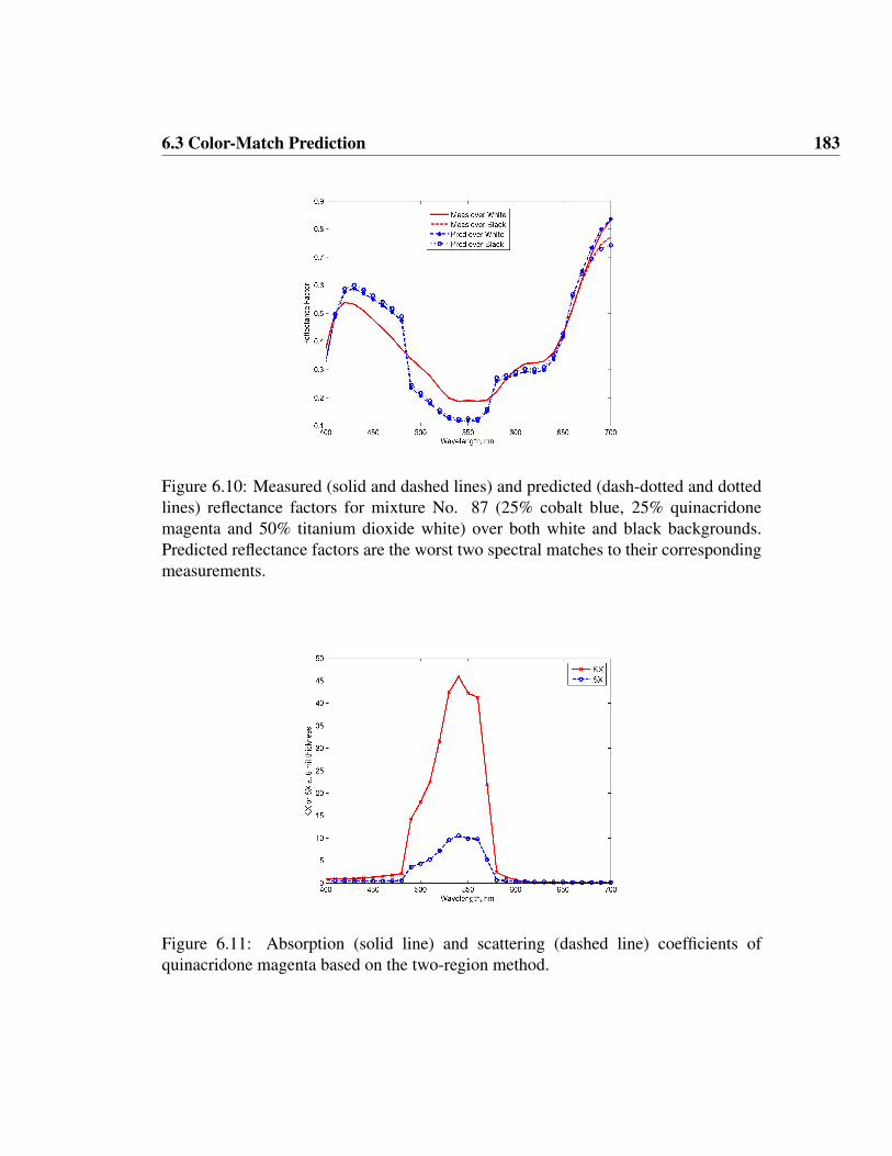
6.3 Color-Match Prediction 183
Figure 6.10: Measured (solid and dashed lines) and predicted (dash-dotted and dottedlines) reflectance factors for mixture No. 87 (25% cobalt blue, 25% quinacridonemagenta and 50% titanium dioxide white) over both white and black backgrounds.Predicted reflectance factors are the worst two spectral matches to their correspondingmeasurements.
Figure 6.11: Absorption (solid line) and scattering (dashed line) coefficients ofquinacridone magenta based on the two-region method.

6.3 Color-Match Prediction 184
This paint fell into the third category of the two-region method when character-
izing its optical constants, i.e., in the opaque region (between 490 and 570 nm), the
masstone-tint method was used, while in translucent regions (below 480 nm and above
580 nm) the black-white method were used. Measured reflectance factors of two mas-
stone drawdowns with the same applicator are plotted in Figure 6.12. There are no-
ticeable differences between these two samples. Despite using the identical technique
for all the drawdowns and training by the manufacturer, it was not possible to control
thickness with sufficient precision. Because the goals of this research were to review
translucent K-M theory and perform an exploratory evaluation, only one masstone
sample and one tint sample were prepared for each paint. The requirement for pre-
cise thickness control based on this evaluation of quinacridone magenta occurred after
the results were analyzed. The absorption and scattering coefficients in the translu-
cent region were sensitive to the variation of film thickness, while these coefficients
in the opaque region were independent of film thickness. Because of thickness varia-
tion of the calibration samples, the absorption and scattering coefficients calculated in
the opaque and translucent regions could not be smoothly connected, even though the
pivot points (490 nm and 570 nm in this example) were smoothed. The imprecision in
characterizing these coefficients in turn affected the color-matching prediction of the
translucent mixture. It is clear that in order to use the K-M theory for translucent ma-
terials, better techniques for controlling film thickness are required as well as multiple
samples and measurements.

6.4 Conclusions 185
Figure 6.12: Measured reflectance factors of two drawdown samples of 100%quinacridone magenta over both backgrounds
6.4 Conclusions
Four methods for determining the absorption and scattering coefficients of translucent
paints have been reviewed including detailed mathematical derivations. They were the
black-white method, the infinite method, the masstone-tint method and the two-region
method. The black-white and infinite methods used the general form of the K-M equa-
tions. The masstone-tint method can be used for both the general form and the opaque
simplification. The two-region method was enhanced in this research and included an
opacity calculation to automatically differentiate opaque and translucent spectral re-
gions. For the opaque region, the masstone-tint method was used; for the translucent
region, the black-white method was used. The black-white method was preferred over
the infinite method because it can be difficult to achieve a paint film that is completely
opaque across the entire visible spectrum. Finally, the pivot point(s) connecting opaque
and translucent regions was smoothed based on a second-order polynomial fitting us-

6.4 Conclusions 186
ing four neighboring points surrounding each pivot point.
The two-region method was used to characterize a set of acrylic-emulsion artist
paints and glazes spanning a range of opacities from opaque to nearly transparent.
Only two calibration drawdowns prepared on an opacity chart were required for this
method, a masstone and a tint. The paints optical constants was tested using mixtures
of a single chromatic paint with either zinc or titanium dioxide white, two chromatic
paints, and two chromatic paints with either zinc or titanium dioxide white. Paint
concentrations were optimized for each test mixture sample over the two backgrounds
under both the opaque and translucent assumptions. The only difference between these
two assumptions was the equation used to calculate reflectance factor from the paints
optical constants. The simplified K-M equation, Eq. (6.2), was used for the opaque
assumption, while the general K-M equation, Eq. (6.1), was used for the translucent
assumption. The paints optical constants and two-constant mixing theory were the
same for these two assumptions.
The test mixture samples were categorized into opaque and translucent groups
based on the average opacity over the entire visible range. For the opaque group,
the opaque and translucent assumptions had negligible difference, while there was a
very large difference between these two assumptions for the translucent group. Fur-
thermore, these two assumptions had a more pronounced difference for samples in the
translucent group over the black background than over the white background.
Performance was reasonable with average colorimetric error of about 4.3 ∆Eab,
RMS spectral error of 1.6% and concentration error of 13% for the mixture sample
in the translucent group. As a comparison, performance was statistically significantly
better with average colorimetric error of about 2.4 ∆Eab, average RMS spectral error
of 1.1% and average concentration error of 7.7% for the mixture samples in the opaque

6.4 Conclusions 187
group. The color-matching prediction for the opaque case was more accurate than that
for the translucent case. It was mainly caused by the variability in film thickness lead-
ing to errors in the optical constants for the translucent films.
The general form of Kubelka-Munk turbid media theory can be applied effectively
to both translucent and opaque paint films providing that sample preparation and spec-
tral measurements have high precision, particularly preparing samples with uniform
and reproducible film thickness.
Chapter 7
Further Investigation of Pigment
Mapping
7.1 Introduction
Multispectral imaging has been originally substantiated within fields such as remote
sensing and geographic information system (GIS). Recently, the technique has been
applied to examine paintings analytically for conservation purposes. In similar fashion
to the identification of land-use classes and the mapping of mineral abundances in re-
mote sensing, multispectral imaging has been used to analyzing pigment composition
of each pixel in a painting. Pigment composition will be beneficial for enriching the
historical knowledge of the painting and will aid conservators in determining the best
course for retouching damaged areas of the painting when metamerism is a factor.
Pigment mapping algorithms are concerned with deconvolving the reflectance spec-
trum of each pixel into its constituent pigments and their concentrations, so the output
is a series of spatial concentration maps of constituent pigments. Since it is difficult

7.1 Introduction 189
and sometimes unachievable to identify the real pigments, the practical goal of pig-
ment mapping is to minimize the root-mean-square (RMS) error between the specified
spectrum and the predicted one from some selected pigments in a predefined database.
One obvious shortcoming of this approach is that it tends to choose more pigments
than necessary to achieve the best match to the specified reflectance spectrum. In order
to alleviate the problem of over-fitting, the number of possible pigments in each pixel
is limited to a certain number (e.g., three or four). In addition, this approach critically
depends on the choice of pigments in the database. If the pigments in the database can
cover the spectral variability of each and every pixel in the painting, pigment mapping
will be successful; otherwise, an unsatisfactory spectral match might result.
The pigment-mixing model describes how to relate the reflectance spectrum of an
unknown pixel to its constituent pigments and their concentrations. The most com-
mon and widely-used model is based on Kubelka-Munk turbid medium theory. It can
be applied for translucent, transparent and opaque films, and also for multiple-layer
films where it is applied sequentially for each layer and treats the reflectance of a
bottom layer as the background reflectance of its top layer. The computation com-
plex increases from transparent, opaque to translucent films, and from single-layer
to multiple-layer configurations. For paintings, the paint layer may be composed of
multiple layers of various thickness and opacities, ranging from transparent glazes to
opaque layers. Some paintings are opaque or completely hide the preparatory ground
layer and canvas, while some are translucent. Also, most paintings consist of multi-
ple layers. For example, a transparent colored glaze may be applied over an opaque
colored layer in specific passages. Also, a transparent varnish layer may be applied
over the whole painting. Since the best spectral match is the goal of pigment mapping,
it is possible to completely ignore the opacity and layer configuration of the painting,

7.2 Experimental Setup 190
and just perform pigment mapping with the simplest model that assumes the painting
consists of a single opaque layer.
The main objective of the chapter is to investigate whether opacity and config-
uration of the painting should be considered or not. Without any knowledge about a
painting, the common practice is to assume that the painting comprises a single opaque
layer. Alternatively, if it is known that the painting is translucent in some areas or it
contains one translucent layer on top of either a translucent or opaque layer, the ques-
tion of whether the extra information may prove useful to improve prediction accuracy
of reflectance spectrum should be answered. Experiments were performed to answer
this question. About 100 paint samples made up of acrylic paints were prepared using
a applicator drawdown bar, encompassing a variety of opacities. Several bi-layer paint
samples were also prepared where the bottom layer was made with acrylic paints and
the top layer was made with color glazes. These samples were measured with both a
in situ spectrophotometer and a spectral-based camera following the application of the
bottom layer and again after the top layer was applied. The results include comparisons
of the prediction accuracy between opaque and translucent assumptions, and between
single and double layer assumptions. The conclusion if opacity and layer configura-
tion information can significantly improve prediction accuracy was drawn from these
comparisons.
7.2 Experimental Setup
Sample preparation Sixteen Golden matte fluid acrylic paints and four colored
glazes were used in this experiment. The optical properties of these paints were char-
acterized on an absolute basis using the two-region method discussed in the previous

7.2 Experimental Setup 191
chapter. Test paint samples were made using a BYK-Gardner applicator bar on Leneta
opacity chart form 3B that had a black region in the middle of two white regions.
Eleven samples were used with a chromatic paint with either zinc or titanium dioxide
white. Fifty-three samples were prepared with two chromatic paints, and another 53
samples were made up of two chromatic paints. So there were 117 paint samples in
total. After these paint films were totally dry, the paint films over both white and black
backgrounds were measured with an integrating spectrophotometer with spectral com-
ponent included. After that, one of the four glazes was selectively applied on top of
each paint film over the black background based on color similarity between glaze and
paint film. Again after the glaze layers were dry, the bi-layer paint films over the black
background were measured.
Preparation of Paint Test Target For each drawdown sample, a square with width
of 1 inch was cut out from both the single film over the white background and the
bi-layer film over the black background. So there were 234 squares in total, and they
were pasted into a black foam core with width of 20 inch and height of 18 inch. The
Golden test target, referred as Small-Square in the next chapter, had thirteen rows and
eighteen columns.
Reflectance Prediction The Sinar camera coupled with two optimized filters was
used in the experiment. The matrix R method discussed in Chapter 3 was used to
transform camera signals to spectral reflectance factor. The camera was perpendicular
to the image plane, and two light sources were placed at 45o apart from either side of
the optical path. This setup simulated 45/0 measurement geometry. All the calibration
and verification targets were also measured with a bi-directional spectrophotometer.
The accuracy of camera prediction is discussed in the next chapter.

7.3 Opaque vs. Translucent 192
7.3 Opaque vs. Translucent
The opaque and translucent assumptions were examined first. In the previous chapter,
it was concluded that the prediction accuracy under translucent assumption was sig-
nificantly higher than that for the opaque assumption. It is worth mentioning that the
conclusion was drawn based on a prior knowledge of paint composition in each mix-
ture sample. If the paint compositions are unknown, whether the same conclusion can
be drawn requires further investigation. Besides spectral and colorimetric accuracies of
pigment mapping, the accuracy of pigment identification was also compared between
the opaque and translucent assumptions. Pigment identification is a proper term here
because the composition information of all these paint samples was available.
Carbon black and raw umber were not used in any mixture sample because they
were spectrally flat or nonselective. Four color glazes were used only in the top layer
of the bi-layer films. Three methods were tested to select three paints out of four-
teen paints to match each single-layer sample, and the objective function for all three
methods was to minimize the spectral RMS error between measured and predicted re-
flectance factors. The only difference between the opaque and translucent assumptions
was how to calculate spectral reflectance factor from the absorption and scattering co-
efficients of the mixture sample.
1. Exhaustive or brute-force search approach For each mixture, all the combina-
tions of three paints from fourteen paints in the database were considered. The
C language was used to speed up the computation time. To bypass the trouble of
writing an optimizing routine to find the optimal concentrations for each combi-
nation, another exhaustive search was done in the concentration domain. Each
concentration varied from 0% to 100% with 5% interval, and only concentration
combinations, where the summation of three paint concentrations was no more

7.3 Opaque vs. Translucent 193
than 100, were used to calculate reflectance factor. First, the optimal concentra-
tions for each 3-paint combinations were obtained with the criterion of minimal
RMS error. Then, the optimal 3-paint combination was found based on the same
criterion.
2. Modified statistical approach This approach was discussed in Chapter 2 (Berns
et al., 2002). The approach required both expert experience and statistical analy-
sis. First, some paints were eliminated from the selection based on expert experi-
ence. Then, a multiple linear regression was performed because single-constant
K-M theory for the opaque case was used. The paints with negative concentra-
tions were eliminated from the model. The process was repeated until all the
concentrations were no less than zero. The modified approach skipped the step
of elimination by expert experience. The objective function was to minimize the
spectral RMS error between measured and predicted reflectance factors, which
were nonlinearly related to the pigment concentrations, so a nonlinear uncon-
strained optimization function ( “fminunc” in MATLAB) was used. In each
iteration, the paints with negative concentrations or the paint with the lowest
concentration was eliminated from the model. The process was repeated until at
most three paints were left in the model.
3. Stepwise nonlinear regression The major difference between this approach and
traditional forward linear stepwise regression was the rule that determined the
entry or removal of each candidate paint. Since the minimum RMS error was
the objective, the improvement of RMS error by entering or removing each can-
didate was calculated. If the improvement of RMS exceeded a certain percentage
(e.g., 15%), the candidate paint was entered into the model, while if the improve-
ment of RMS was less than a certain percentage (e.g., 20%), the candidate paint

7.3 Opaque vs. Translucent 194
was removed from the model. Also at most three paints were selected. The
paint concentrations were fully constrained and optimized with the optimization
function (“fmincon” in MATLAB).
The computation speed for the exhaustive search was the fastest, because it was
written in C language and the other two methods depended on the optimization func-
tions in MATLAB. Also, the exhaustive search provided the highest accuracies for
both pigment identification and mapping. Since the purpose was not to develop a new
robust approach, the exhaustive search approach was used in the following discussion
and in the next chapter.
7.3.1 Prior Knowledge of Constituent Pigments
In this section, it was assumed that constituent pigments in each mixture were known.
So pigment identification was skipped, only the accuracy of pigment mapping was
evaluated. Three different cases were discussed.
Nominal Concentration These paint samples were prepared carefully on contrast pa-
per. For each paint sample, the constituent pigments and their concentrations
were known. This concentration based on weight measurement was referred as
the nominal concentration. The reflectance factor of each paint sample was cal-
culated using the optical properties of its constituent pigments and their nominal
concentrations, and compared with the corresponding spectrophotometric mea-
surement. In this way, the accuracy of the forward pigment-mixing model was
evaluated.
Optimized Concentration The constituent pigments in each sample were known, but
their concentrations were optimized to minimize the spectral RMS error between

7.3 Opaque vs. Translucent 195
measured and predicted reflectance factors from the pigment-mixing model. The
nominal concentration might be erroneous because of the weighting imprecision,
incomplete mixing and non-uniformity of the film. For example, given that the
repeatability of the scale was 0.01g, if the total weight of the mixture was 5g, the
concentration precision was 0.2%. The accuracy of the forward pigment-mixing
model should be better evaluated when the optimized concentrations, instead
of the nominal concentrations, were used to estimate spectral reflectance factor
from the optical properties of the constituent pigments.
Quantized Concentration The optimized concentrations were quantized to the preci-
sion of 5%. The simple operation was to divide the concentration by 0.05, round
the quotient to the nearest integer, and then multiply by 0.05. The concentra-
tion precision in the exhaustive search approach was 5%, and this case was to
examine whether this precision was sufficient.
The opaque and translucent assumptions were first tested with the 117 single-layer
paint samples over both a white and a black background given that the constituent
pigments were known. The accuracy metrics for the forward pigment-mixing model
included simple and complex color difference equations calculated for CIE illumi-
nant D65 and the 10-degree observer, ∆Eab and ∆E00, spectral RMS error (%) and a
metameric index from CIE illuminant D65 to A.
7.3.1.1 Single-Layer Samples Over the White Background
The statistical results of the prediction accuracies of the single-layer paint samples over
the white background for the opaque assumption are listed in Table 7.1. Several useful
conclusions could be drawn:
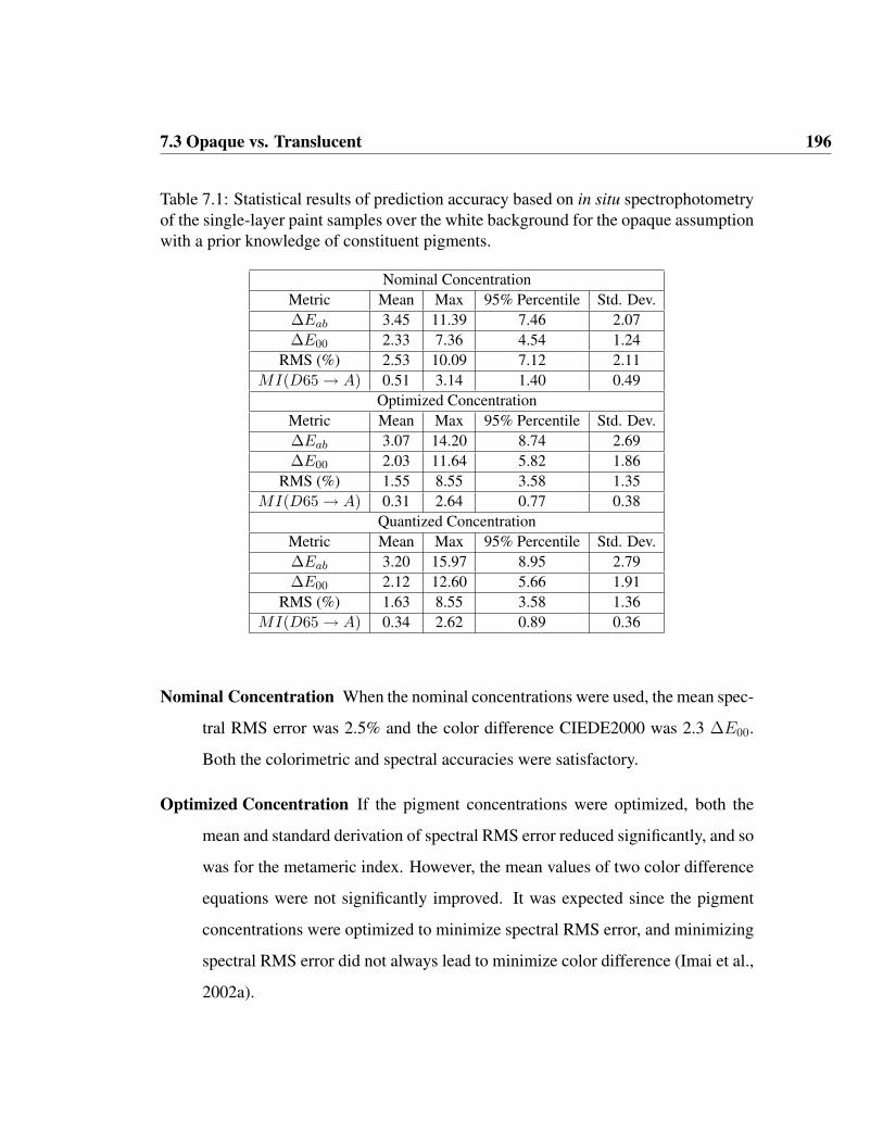
7.3 Opaque vs. Translucent 196
Table 7.1: Statistical results of prediction accuracy based on in situ spectrophotometryof the single-layer paint samples over the white background for the opaque assumptionwith a prior knowledge of constituent pigments.
Nominal ConcentrationMetric Mean Max 95% Percentile Std. Dev.∆Eab 3.45 11.39 7.46 2.07∆E00 2.33 7.36 4.54 1.24
RMS (%) 2.53 10.09 7.12 2.11MI(D65 → A) 0.51 3.14 1.40 0.49
Optimized ConcentrationMetric Mean Max 95% Percentile Std. Dev.∆Eab 3.07 14.20 8.74 2.69∆E00 2.03 11.64 5.82 1.86
RMS (%) 1.55 8.55 3.58 1.35MI(D65 → A) 0.31 2.64 0.77 0.38
Quantized ConcentrationMetric Mean Max 95% Percentile Std. Dev.∆Eab 3.20 15.97 8.95 2.79∆E00 2.12 12.60 5.66 1.91
RMS (%) 1.63 8.55 3.58 1.36MI(D65 → A) 0.34 2.62 0.89 0.36
Nominal Concentration When the nominal concentrations were used, the mean spec-
tral RMS error was 2.5% and the color difference CIEDE2000 was 2.3 ∆E00.
Both the colorimetric and spectral accuracies were satisfactory.
Optimized Concentration If the pigment concentrations were optimized, both the
mean and standard derivation of spectral RMS error reduced significantly, and so
was for the metameric index. However, the mean values of two color difference
equations were not significantly improved. It was expected since the pigment
concentrations were optimized to minimize spectral RMS error, and minimizing
spectral RMS error did not always lead to minimize color difference (Imai et al.,
2002a).
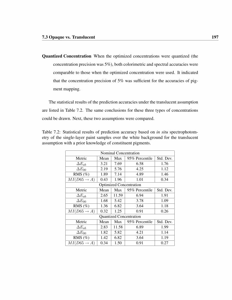
7.3 Opaque vs. Translucent 197
Quantized Concentration When the optimized concentrations were quantized (the
concentration precision was 5%), both colorimetric and spectral accuracies were
comparable to those when the optimized concentration were used. It indicated
that the concentration precision of 5% was sufficient for the accuracies of pig-
ment mapping.
The statistical results of the prediction accuracies under the translucent assumption
are listed in Table 7.2. The same conclusions for these three types of concentrations
could be drawn. Next, these two assumptions were compared.
Table 7.2: Statistical results of prediction accuracy based on in situ spectrophotom-etry of the single-layer paint samples over the white background for the translucentassumption with a prior knowledge of constituent pigments.
Nominal ConcentrationMetric Mean Max 95% Percentile Std. Dev.∆Eab 3.21 7.69 6.58 1.76∆E00 2.19 5.76 4.25 1.12
RMS (%) 1.89 7.14 4.89 1.46MI(D65 → A) 0.43 1.96 1.01 0.34
Optimized ConcentrationMetric Mean Max 95% Percentile Std. Dev.∆Eab 2.65 11.59 6.94 1.91∆E00 1.68 5.42 3.78 1.09
RMS (%) 1.36 6.82 3.64 1.18MI(D65 → A) 0.32 1.25 0.91 0.26
Quantized ConcentrationMetric Mean Max 95% Percentile Std. Dev.∆Eab 2.83 11.58 6.89 1.99∆E00 1.82 5.82 4.21 1.14
RMS (%) 1.42 6.82 3.64 1.19MI(D65 → A) 0.34 1.50 0.91 0.27

7.3 Opaque vs. Translucent 198
Almost all the statistical values in Table 7.2 were smaller than those in Table 7.1.
The student t-test was used to test whether the means of two groups were significantly
different from each other at a certain significant level α (0.05). For the nominal con-
centration, the spectral RMS error under the translucent assumption was significantly
smaller than that for the opaque assumption. For the optimized concentration, the color
difference CIEDE2000 under the translucent assumption was better. For the quantized
concentration, all the error metrics were not significantly better. So the translucent as-
sumption was only slightly superior to the opaque assumption, which was unexpected.
One major reason was that the translucent model was sensitive to the variation of the
film thickness. It was assumed that all the drawdown samples had the same wet thick-
ness since all the samples were prepared with an applicator with an opening of 6mil.
However, it was practically difficult to achieve. The thickness variation could affect the
accuracy of the pigment mapping directly or indirect through error propagation from
the inaccuracy of the pigment constants. For example, the mixture of hansa yellow
medium and zinc white happened to be the worst spectral match. The measured and
predicted reflectance factors for this sample under these two assumptions are plotted
in Figure 7.1. The predicted reflectance factors under the translucent assumption at the
longer wavelength had the same wave-like shape as the measurement, which was char-
acteristic of spectral reflectance factor of the white background of the opacity chart
[Figure 6.3(a)], but the spectral curves were obviously lower than the measurement.
The thickness variation of the sample might cause this shift. Other possible reasons
might be the imperfectness of the K-M theory for the translucent case, the inaccuracy
of the pigment database using the two-region method, and imprecision of reflectance
measurement.

7.3 Opaque vs. Translucent 199
380 430 480 530 580 630 680 7300
0.2
0.4
0.6
0.8
1
Wavelength,nm
Ref
lect
ance
Fac
tor
MeasuredNorminal ConcentrationOptimized ConcentrationQuantized Concentration
(a) Opaque Assumption
380 430 480 530 580 630 680 7300
0.2
0.4
0.6
0.8
1
Wavelength,nm
Ref
lect
ance
Fac
tor
MeasuredNorminal ConcentrationOptimized ConcentrationQuantized Concentration
(b) Translucent Assumption
Figure 7.1: Measured and predicted reflectance factors for a mixture sample of hansayellow medium and zinc white over the white background under the opaque andtranslucent assumptions.
7.3.1.2 Single-Layer Samples Over the Black Background
The opaque and translucent assumptions were compared for the single-layer samples
over the black background with a prior knowledge of constituent pigments. The sta-
tistical results under these two assumptions were listed in Tables 7.3 and 7.4. Several
useful observations were summarized as follows:
• Under the opaque assumption, the colorimetric accuracy was significantly worse
when the optimized concentrations were used to estimate the reflectance fac-
tors, although the spectral accuracy improved slightly. The results based on the
quantized concentrations were not different from those when the optimized con-
centrations were used.
• Under the translucent assumption, both colorimetric and spectral accuracies im-
proved when the optimized concentrations were used. Again, quantization of the
optimized concentrations did not affect the accuracy of pigment mapping.

7.3 Opaque vs. Translucent 200
• For all the error metrics and all three types of concentrations, both the means and
standard derivations under the translucent assumption were significantly smaller
than those for the opaque assumption. The conclusions drawn from the same
samples over two different backgrounds were quite different.
Table 7.3: Statistical results of prediction accuracy based on in situ spectrophotometryof the single-layer paint samples over the black background for the opaque assumptionwith a prior knowledge of constituent pigments.
Nominal ConcentrationMetric Mean Max 95% Percentile Std. Dev.∆Eab 4.01 32.47 9.43 4.01∆E00 2.43 14.86 5.27 1.82
RMS (%) 4.40 32.81 20.34 6.32MI(D65 → A) 0.63 4.21 2.89 0.83
Optimized ConcentrationMetric Mean Max 95% Percentile Std. Dev.∆Eab 5.16 44.68 21.86 7.13∆E00 3.37 21.11 14.55 4.22
RMS (%) 3.28 29.62 17.66 5.37MI(D65 → A) 0.55 4.22 2.51 0.75
Quantized ConcentrationMetric Mean Max 95% Percentile Std. Dev.∆Eab 5.20 44.68 20.66 7.07∆E00 3.37 20.85 14.04 4.15
RMS (%) 3.31 29.62 17.66 5.37MI(D65 → A) 0.56 4.29 2.52 0.76

7.3 Opaque vs. Translucent 201
Table 7.4: Statistical results of prediction accuracy based on in situ spectrophotom-etry of the single-layer paint samples over the black background for the translucentassumption with a prior knowledge of constituent pigments.
Nominal ConcentrationMetric Mean Max 95% Percentile Std. Dev.∆Eab 3.06 7.64 6.00 1.64∆E00 2.09 5.75 4.00 1.06
RMS (%) 1.56 5.30 4.08 1.21MI(D65 → A) 0.38 1.66 0.94 0.31
Optimized ConcentrationMetric Mean Max 95% Percentile Std. Dev.∆Eab 2.20 8.23 4.84 1.41∆E00 1.44 4.91 2.89 0.85
RMS (%) 1.01 3.85 2.59 0.79MI(D65 → A) 0.25 0.80 0.69 0.20
Quantized ConcentrationMetric Mean Max 95% Percentile Std. Dev.∆Eab 2.41 8.63 4.83 1.48∆E00 1.61 5.10 3.24 0.93
RMS (%) 1.07 4.58 2.62 0.83MI(D65 → A) 0.27 0.94 0.70 0.20
Next, it will be investigated the reason why the accuracy of pigment mapping im-
proved greatly for the samples over the black background, but not for the same sam-
ples over the white background. The effect of the white background for the translucent
sample might be equivalent to adding white paint into the sample. Similarly, the black
background might be exchangeable with the black paint. The opaque assumption as-
sumed that the paint samples were totally hidden the background, which was not true
for some samples. In order to take the effect of black background into account, it might
be necessary to incorporate carbon black into the pigment-mixing model as an extra
component. Statistical results for the prediction accuracy when the carbon black is
incorporated are listed in Table 7.5. Several important observations were summarized

7.3 Opaque vs. Translucent 202
as follows,
Table 7.5: Statistical results of prediction accuracy based on in situ spectrophotometryof the single-layer paint samples over the black background for the opaque assumptionwith a prior knowledge of constituent pigments and incorporating carbon black as anextra component.
Optimized ConcentrationMetric Mean Max 95% Percentile Std. Dev.∆Eab 2.20 9.15 5.96 1.80∆E00 1.41 5.45 3.41 1.03
RMS (%) 0.90 3.08 2.22 0.70MI(D65 → A) 0.26 1.01 0.79 0.23
Quantized ConcentrationMetric Mean Max 95% Percentile Std. Dev.∆Eab 3.77 28.79 11.97 4.26∆E00 2.24 14.33 6.34 2.12
RMS (%) 4.84 33.24 20.42 6.81MI(D65 → A) 0.76 6.10 3.31 1.07
• Both colorimetric and spectral accuracies of the pigment mapping with the op-
timized concentrations were significantly improved when the carbon black were
incorporated. The mean color difference CIEDE2000 became 1.4 ∆E00, and the
mean spectral RMS error was below 1%. All the error metrics under the opaque
assumption were comparable to those under the translucent assumption.
• However, when the optimized concentrations were quantized, the colorimetric
accuracy was improved, while the spectral accuracy was worse. This was caused
by quantization error of concentration for the black paint. The example of a mix-
ture of hansa yellow medium and zinc white was analyzed again. Measured and
predicted reflectance factors for this sample under both assumptions are plotted
in Figure 7.2. Under the opaque assumption, the predicted reflectance factors

7.3 Opaque vs. Translucent 203
from the nominal and quantized concentrations were too bigger than the corre-
sponding measurements at the longer wavelengths, while the spectral curve from
the optimized concentration was much closer to the measurement. The opti-
mized concentrations were 10.6% hansa yellow medium, 89.3% zinc white and
0.1% carbon black. After quantization, the concentrations became 10% hansa
yellow medium and 90% zinc white. The tiny amount of carbon black caused
the huge difference of reflectance factors between the optimized and quantized
concentrations. So the concentration precision of 5% was not sufficient for the
black paint. Again the practical concentration precision based on weighting was
0.2%. So it was impractical to mix the accurate amount of the black paint in
the mixture. In addition, the predicted reflectance factor under the translucent
assumption was matched to the measurement much better.
380 430 480 530 580 630 680 7300
0.2
0.4
0.6
0.8
1
Wavelength,nm
Ref
lect
ance
Fac
tor
MeasuredNorminal ConcentrationOptimized ConcentrationQuantized Concentration
(a) Opaque Assumption
380 430 480 530 580 630 680 7300
0.1
0.2
0.3
0.4
0.5
0.6
0.7
Wavelength,nm
Ref
lect
ance
Fac
tor
Measured
Norminal Concentration
Optimized Concentration
Quantized Concentration
(b) Translucent Assumption
Figure 7.2: Measured and predicted reflectance factors for a mixture sample of hansayellow medium and zinc white over the black background under the opaque andtranslucent assumptions. Carbon black was added for the opaque assumption.

7.3 Opaque vs. Translucent 204
7.3.1.3 Summary
With a prior knowledge of constituent pigments (100% accuracy of pigment identifi-
cation), the accuracy of pigment mapping was analyzed separately. The reflectance
factors were calculated from three types of concentrations, and they were nominal,
optimized and quantized concentrations. For the samples over the white background,
the translucent assumption was just slightly superior to the opaque assumption, and
the concentration precision of 5% was sufficient. On the other hand, for the the same
samples over the black background, it seemed that the translucent assumption was
significantly better. But it was not true. The effect of black background was equiv-
alent to adding the black paint in the paint samples. Superiority of the translucent
assumption was lost when carbon black was incorporated as an extra component in the
pigment-mixing model under the opaque assumption. The tiny amount of carbon black
caused the huge difference in reflectance factors. The requirement of the concentra-
tion precision for the black paint was even stricter than the practical precision based
on weighting. In a word, if both black and white paints were incorporated into the
pigment-mixing model for the opaque case, no significant difference existed between
the opaque and translucent assumptions as far as the accuracy of pigment mapping was
concerned.
7.3.2 Spectrophotometric Measurement
Next, the constituent pigments were not inputted in the pigment-mixing model. The
exhaustive search approach was used to find the best combination of pigments and
the best concentration for each paint sample. The opaque and translucent assumptions
were first compared based upon in situ spectrophotometry, and then spectral-based
camera, which incorporated the inaccuracy of spectral prediction from the camera sys-

7.3 Opaque vs. Translucent 205
tem. The single-layer paint films over both a white and a black background were
measured with in situ spectrophotometry. First, the comparisons were done for the
single-layer films over a white background, and followed by over a black background.
The accuracy metric for pigment identification was the number of misidentified
paints. These paints were mixed with either one of two whites (zinc white and titanium
dioxide white) or no white. Since it was very hard to identify the existence or type of
white paint, the misidentification of the white paint was not considered. Number ”0”
means that all the chromatic paints were successfully identified. The other numbers
mean that the identified paints were either redundant or misidentified. The percentage
of error was defined as the ratio between the number of wrong identified paints and
the total number of paints. There were 106 mixtures made up of two chromatic paints
and 11 mixtures of one chromatic paints, so the total number of chromatic paints was
106× 2 + 11 = 223.
7.3.2.1 Single-Layer Samples Over the White Background
Accuracies of both pigment identification and mapping are listed in Tables 7.6 and 7.7,
respectively. The total number of misidentified paints under the translucent assumption
was less than that under the opaque assumption. Both the means and standard deriva-
tions for all four error metrics under the translucent assumption were smaller. Further
statistical analysis was needed to determine whether these differences were significant.

7.3 Opaque vs. Translucent 206
Table 7.6: Accuracy of pigment identification based on in situ spectrophotometry ofthe single-layer paint samples over the white background under opaque and translucentassumptions.
No. of misidentified paintsAssumption 0 1 2 3 Total % error
opaque 73 28 13 3 1x28+2x13+3x3 = 63 63/223≈28%translucent 76 37 3 1 1x37+2x3+1x3 = 46 46/223≈21%
Table 7.7: Statistical results of prediction accuracy based on in situ spectrophotometryof the single-layer paint samples over the white background under both opaque andtranslucent assumptions.
Opaque AssumptionMetric Mean Max 95% Percentile Std. Dev.∆Eab 2.81 11.44 7.60 2.20∆E00 1.83 7.12 5.14 1.45
RMS (%) 1.22 4.53 2.80 0.89MI(D65 → A) 0.32 2.55 0.89 0.34
Translucent AssumptionMetric Mean Max 95% Percentile Std. Dev.∆Eab 2.52 6.92 5.34 1.54∆E00 1.61 5.71 3.58 1.06
RMS (%) 0.98 3.49 2.53 0.72MI(D65 → A) 0.25 1.02 0.88 0.22
The F-test was used to test whether the standard derivations of the two groups were
significantly different, while the student T-test was used to test whether the means
of these two groups were significantly different. The results of statistical tests were
summarized in Table 7.8. Symbol “0 means that the null hypothesis that two values
are the same is accepted at a 95% confidence level, while symbol “1 means that the
null hypothesis is rejected. The standard derivations between two assumptions for all
error metrics were significantly different, and only the mean value of RMS error under

7.3 Opaque vs. Translucent 207
translucent sample was statistically smaller than that under opaque assumption.
Table 7.8: Results of statistical tests between opaque and translucent assumptionsbased on in situ spectrophotometry of the single-layer paint samples over the whitebackground. Symbol “0 means that the null hypothesis that two values are the same isaccepted at a 95% confidence level, while symbol “1 means that the null hypothesis isrejected.
Statistical Test Identification ∆Eab ∆E00 RMS (%) MI(D65 → A)F-test 1 1 1 1 1T-test 0 0 0 1 0
Under the translucent assumption, pigment identification for one sample was un-
successful, since all three paints were misidentified. This sample was actually made
up of ultramarine blue, red oxide and zinc white, but the program found the combina-
tion of chromium oxide green, yellow ochre and quinacridone magenta was the best
combination to match the measured reflectance factor of this sample. The reflectance
factors were calculated from the known and optimized paint combinations, and the
concentrations for both combinations were optimized using the optimization function
in MATLAB. The measured and predicted factors are plotted in Figure 7.3. The RMS
errors were calculated between measured and reflectance factors predicted from these
two compositions, and they were 1.55% and 1.64% for the known and optimized com-
positions, respectively. This small RMS difference made it difficult to find the right
composition for this sample. The RMS error for predicted reflectance factor from the
optimized combination using the exhaustive search was slightly worse because of the
imprecision of paint concentrations (5%). It was obvious that the predicted reflectance
factor from the known paint composition did not match the corresponding measure-
ment either. The prediction of reflectance factors from the known composition was
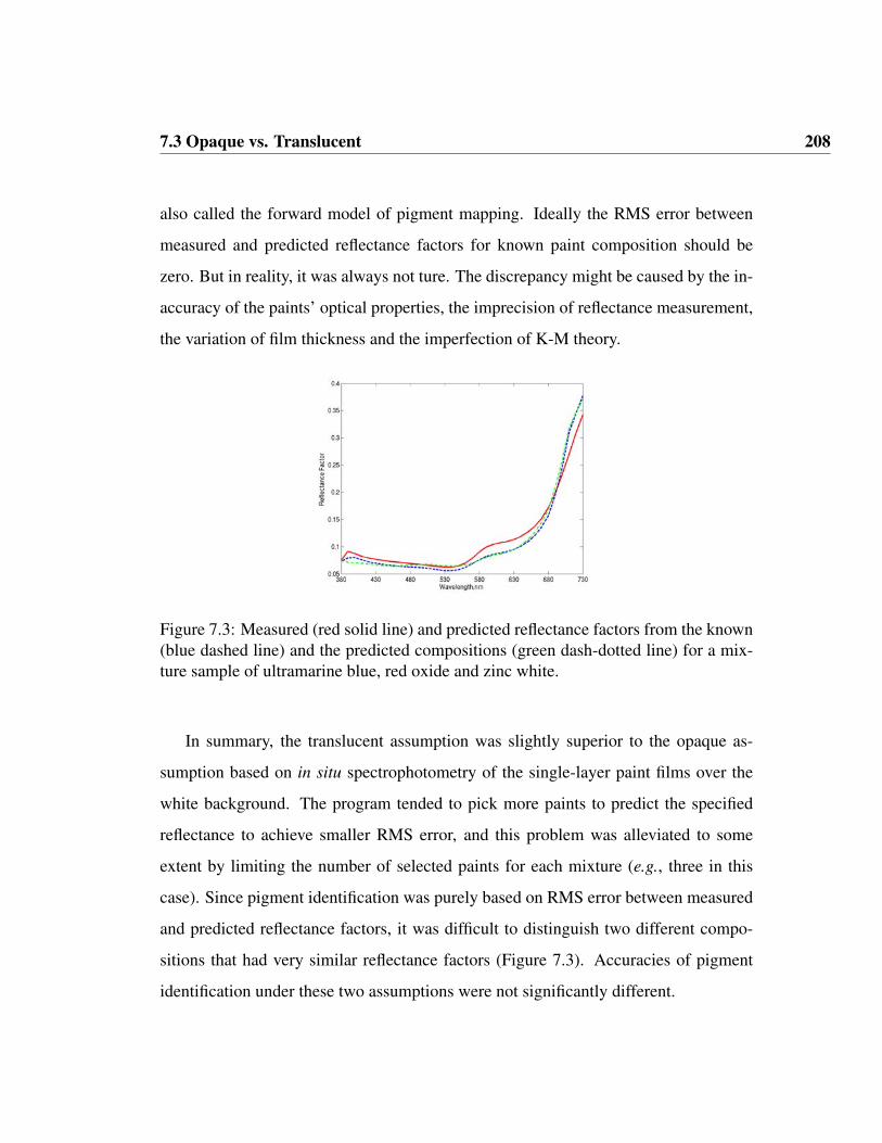
7.3 Opaque vs. Translucent 208
also called the forward model of pigment mapping. Ideally the RMS error between
measured and predicted reflectance factors for known paint composition should be
zero. But in reality, it was always not ture. The discrepancy might be caused by the in-
accuracy of the paints’ optical properties, the imprecision of reflectance measurement,
the variation of film thickness and the imperfection of K-M theory.
Figure 7.3: Measured (red solid line) and predicted reflectance factors from the known(blue dashed line) and the predicted compositions (green dash-dotted line) for a mix-ture sample of ultramarine blue, red oxide and zinc white.
In summary, the translucent assumption was slightly superior to the opaque as-
sumption based on in situ spectrophotometry of the single-layer paint films over the
white background. The program tended to pick more paints to predict the specified
reflectance to achieve smaller RMS error, and this problem was alleviated to some
extent by limiting the number of selected paints for each mixture (e.g., three in this
case). Since pigment identification was purely based on RMS error between measured
and predicted reflectance factors, it was difficult to distinguish two different compo-
sitions that had very similar reflectance factors (Figure 7.3). Accuracies of pigment
identification under these two assumptions were not significantly different.

7.3 Opaque vs. Translucent 209
7.3.2.2 Single-Layer Samples Over the Black Background
Next, the single-layer paint samples over a black background were examined. The
accuracies of pigment identification and mapping are listed in Tables 7.9 and 7.10. The
total number of misidentified paints under the translucent assumption was less than half
of that under the opaque assumption. All the statistical results for all the error metrics
under translucent assumption were smaller than those under opaque assumption. The
means and standard derivations under these two assumptions were statistically different
for all the error metrics, as listed in Table 7.11.
Table 7.9: Accuracy of pigment identification based on in situ spectrophotometry ofthe single-layer paint samples over the black background under opaque and translucentassumptions.
No. of misidentified paintsAssumption 0 1 2 3 Total % Error
opaque 51 50 16 0 1x50+2x16 = 82 82/223≈37%translucent 83 30 4 0 1x30+2x4 = 38 38/223≈17%

7.3 Opaque vs. Translucent 210
Table 7.10: Statistical results of prediction accuracy based on in situ spectrophotome-try of the single-layer paint samples over the black background under both opaque andtranslucent assumptions.
Opaque AssumptionMetric Mean Max 95% Percentile Std. Dev.∆Eab 3.12 17.67 8.07 2.72∆E00 1.98 8.09 4.99 1.58
RMS (%) 1.38 7.39 3.93 1.28MI(D65 → A) 0.34 1.30 0.95 0.28
Translucent AssumptionMetric Mean Max 95% Percentile Std. Dev.∆Eab 2.15 6.48 5.02 1.39∆E00 1.38 4.22 3.03 0.86
RMS (%) 0.91 3.47 2.53 0.73MI(D65 → A) 0.23 0.94 0.63 0.19
Table 7.11: Results of statistical test between opaque and translucent assumptionsbased on in situ spectrophotometry of the single-layer paint samples over the blackbackground. Symbol “0 means that the null hypothesis that two values are the same isaccepted at a 95% confidence level, while symbol “1 means that the null hypothesis isrejected.
Statistical Test Identification ∆Eab ∆E00 RMS (%) MI(D65 → A)F-test 1 1 1 1 1T-test 1 1 1 1 1
Under the translucent assumption, there were four mixtures that had two misidenti-
fied paints (Table 7.9). The known and predicted paint compositions under translucent
assumption for these mixtures are listed in Table 7.12, along with spectral RMS er-
rors between measured and predicted reflectance factors from the known and predicted
compositions. The measured and predicted reflectance factors from the known and
predicted compositions are plotted in Figure 7.4.

7.3 Opaque vs. Translucent 211
Table 7.12: Four examples of known and predicted paint compositions under translu-cent assumption based on in situ spectrophotometry of the single-layer samples overthe black background.
Known Composition Predicted CompositionNo. Paints RMS (%) Paints RMS (%)
Pyrrole Red Chromium Oxide Green1 Zinc White 3.22 Quinacridone Magenta 2.04
Zinc WhiteQuinacridone Magenta Quinacridone Magenta
2 Green Gold 1.14 Raw Umber 0.90Hansa Yellow Medium
Diarylide Yellow Diarylide Yellow3 Ultramarine Blue 1.34 Chromium Oxide Green 1.43
Zinc White Quinacridone MagentaPyrrole Red Pyrrole Red
4 Green Gold 1.02 Yellow Ochre 1.80Zinc White Hansa Yellow Medium
For the last two samples, the RMS errors for predicted compositions were higher
than those for the known compositions. It was caused by the 5% step size used for
concentrations in the exhaustive search method. For the first two samples, misidenti-
fication might stem from optimization objective that was to minimize the RMS error.
The reasons for the discrepancy between measured and predicted from the known com-
position was discussed above.
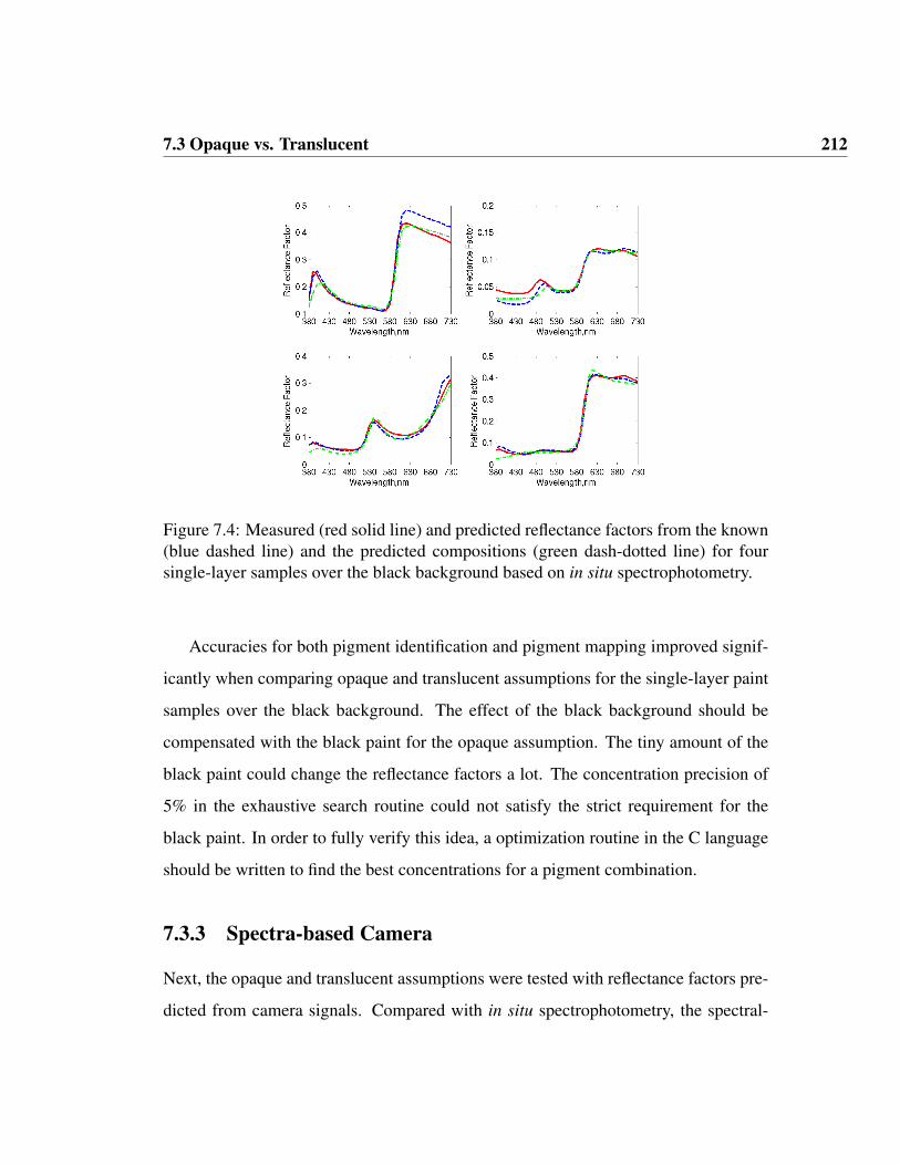
7.3 Opaque vs. Translucent 212
Figure 7.4: Measured (red solid line) and predicted reflectance factors from the known(blue dashed line) and the predicted compositions (green dash-dotted line) for foursingle-layer samples over the black background based on in situ spectrophotometry.
Accuracies for both pigment identification and pigment mapping improved signif-
icantly when comparing opaque and translucent assumptions for the single-layer paint
samples over the black background. The effect of the black background should be
compensated with the black paint for the opaque assumption. The tiny amount of the
black paint could change the reflectance factors a lot. The concentration precision of
5% in the exhaustive search routine could not satisfy the strict requirement for the
black paint. In order to fully verify this idea, a optimization routine in the C language
should be written to find the best concentrations for a pigment combination.
7.3.3 Spectra-based Camera
Next, the opaque and translucent assumptions were tested with reflectance factors pre-
dicted from camera signals. Compared with in situ spectrophotometry, the spectral-

7.3 Opaque vs. Translucent 213
based camera incorporated the inaccuracy of spectral prediction of the camera system.
The Golden Small-Square target had 234 patches. Half of all the patches were single-
layer samples over the white background, while the other half were bi-layer samples
over the black background. The reflectance factors for this target were predicted from
camera signals. It is better to separate the discussion of opacity from layer configu-
ration. In this section, the opaque and translucent assumptions were only tested with
single-layer samples over the white background.
The accuracies of pigment identification and mapping were very similar for these
two assumptions, as shown in Tables 7.13 and 7.14. The means and standard deriva-
tions were not statistically different under these two assumptions for all error metrics
(Table 7.15). It was concluded that these two assumptions were virtually the same for
the spectral-based camera. Thus, the opaque assumption should be used instead of
translucent assumption for several reasons. First, sample preparation could be greatly
simplified without the need to accurately control the film thickness. Second, paint
characterization was much easier. Third and the most importantly, the pigment map-
ping can be treated as a linear mixing problem in term of the ratio of absorption and
scattering coefficients.
Table 7.13: Accuracy of pigment identification based on spectral-based camera of thesingle-layer paint samples over the white background under opaque and translucentassumptions.
No. of misidentified paintsAssumption 0 1 2 3 Total % Error
opaque 34 45 35 3 1x45+2x35+3x3 = 124 124/223≈56%translucent 34 49 30 4 1x49+2x30+3x4 = 121 121/223≈54%

7.3 Opaque vs. Translucent 214
Table 7.14: Statistical results of prediction accuracy based on spectral-based cameraof the single-layer paint samples over the white background under both opaque andtranslucent assumptions.
Opaque AssumptionMetric Mean Max 95% Percentile Std. Dev.∆Eab 5.56 19.06 13.29 3.76∆E00 3.63 17.52 9.20 2.79
RMS (%) 2.06 5.57 4.33 1.08MI(D65 → A) 0.66 2.46 1.75 0.51
Translucent AssumptionMetric Mean Max 95% Percentile Std. Dev.∆Eab 5.60 22.74 11.49 3.61∆E00 3.59 19.88 9.04 2.82
RMS (%) 2.10 6.21 4.82 1.18MI(D65 → A) 0.64 3.25 2.05 0.59
Table 7.15: Results of statistical tests between opaque and translucent assumptionsbased on spectral-based camera of the single-layer paint samples over the white back-ground. Symbol “0 means that the null hypothesis that two values are the same isaccepted at a 95% confidence level, while symbol “1 means that the null hypothesis isrejected.
Statistical Test Identification ∆Eab ∆E00 RMS (%) MI(D65 → A)F-test 0 0 0 0 0T-test 0 0 0 0 0
Next, four mixture samples that had three misidentified paints under translucent
assumption warrants more detailed discussion (Table 7.13). The known and predicted
compositions for these samples are listed in Table 7.16. The measured and predicted
reflectance factors from those two compositions are plotted in Figure 7.5. The re-
flectance factors from the predicted compositions were actually more similar to those
from the known composition. It was worth mentioning that the measured reflectance

7.3 Opaque vs. Translucent 215
factors were actually predicted from camera signals. These four mixture samples were
all dark colors. It is known that the camera prediction for dark color is problematic
since the spectral RMS error between measured and predicted reflectance factors was
small for dark colors.
Table 7.16: Four examples of the known and predicted paint compositions undertranslucent assumption based on spectra-based camera.
Known Composition Predicted CompositionNo. Paints RMS (%) Paints RMS (%)
Ultramarine Blue Cobalt Blue1 Yellow Ochre 1.84 Chromium Oxide Green 1.28
Raw UmberUltramarine Blue Cobalt Blue
2 Hansa Yellow Medium 2.04 Green Gold 1.58Raw Umber
Cobalt Blue Quinacridone Magenta3 Red Oxide 2.15 Chromium Oxide Green 2.66
Burnt SiennaPhthalo Green Ultramarine Blue
4 Burnt Sienna 0.99 Yellow Ochre 0.80Raw Umber

7.3 Opaque vs. Translucent 216
Figure 7.5: Measured (red solid line) and predicted reflectance factors from the known(blue dashed line) and the predicted compositions (green dash-dotted line) for foursingle-layer samples over the white background based on spectral-based camera.
In summary, the opaque and translucent assumptions were virtually the same for
single-layer paint samples based on the spectral-based camera. This conclusion coin-
cided with that drawn from the same samples measured with the spectrophotometric
measurements. Based on the spectrophotometric measurements, these two assump-
tions were slightly different for single-layer samples over the white background, and
significantly different for single-layer samples over the black white background. Most
paintings were drawn over white canvas and measured via the spectra-based camera,
and paint composition information for each pixel was unavailable. Thus, it is sug-
gested that simple opaque assumption is a reasonable choice for pigment mappings of
paintings.

7.4 Single-Layer vs. Bi-Layer 217
7.4 Single-Layer vs. Bi-Layer
In this secion, the single-layer and bi-layer assumptions were examined. There were
117 bi-layer samples in total, that were painted over the black background only. The
bottom layer was made of acrylic paints, and the top layer contained only one colored
glaze. For single-layer assumption, the same program as above could be used, while
for the bi-layer assumption, more discussions were necessary. Reflectance factor pre-
dicted from the bottom layer was treated as background reflectance factor for the top
layer. For the bottom layer, the same program as above was used, while for the top
layer, another loop was incorporated to go through four colored glazes. Due to the
difficulty to keep the top layer the same thickness, the thickness for the top layer var-
ied from 0.5 to 1.5 with 0.25 increments. The bi-layer configurations were tested with
these bi-layer samples over the black background. Since opacity and translucent as-
sumptions were significantly different for samples over the black background based on
spectrophotometric measurements discussed earlier, the translucent assumption was
made for both the bottom and top layer. The runtime for each patch was about 10
seconds.
7.4.1 Prior Knowledge of Constituent Pigments
The single-layer and bi-layer assumptions were first compared when constituent pig-
ments and layer configuration were known. Under the single-layer assumption, only
the pigments in the bottom layer were available, and their concentrations were opti-
mized to minimize spectral RMS error. On the other hand, for the bi-layer assumption,
both component pigments in the bottom layer and glaze in the top layer were inputted
into the pigment-mixing model. The glaze was applied after the first layer was totally

7.4 Single-Layer vs. Bi-Layer 218
dry. Due to difficulty of controlling the thickness of the glaze layer, the thickness of
the glaze was also optimized along with the concentrations of component pigments in
the bottom layer. Both layers were assumed to be translucent, so the general form of
K-M theory for the translucent case was used.
The statistical results of pigment mapping under the single-layer and bi-layer as-
sumptions are listed in Table 7.17. Under the single-layer assumption, the glaze layer
was totally discarded, and only the constituent pigments in the bottom layer were used
to estimate the reflectance factor of the bi-layer paint sample. Under the bi-layer as-
sumption, the constituent pigments in the bottom layer and glazes in the top layer were
known. Both the pigment concentrations and the thickness of the glaze layer were op-
timzied. The mean color difference was about 2 ∆E00, and the spectral RMS error was
1.1%. Both colorimetric and spectral accuracies under the bi-layer assumption were
significantly better than those for the single-layer assumption. It was expected since
the glaze layer was considered under the bi-layer assumption.
Table 7.17: Statistical results of prediction accuracy based on the bi-layer paint sam-ples over the black background under both single-layer and bi-layer assumptions.
Single-layer AssumptionMetric Mean Max 95% Percentile Std. Dev.∆Eab 7.57 37.44 15.29 5.61∆E00 4.33 20.50 9.10 2.88
RMS (%) 1.81 9.51 4.19 1.48MI(D65 → A) 0.65 2.50 1.77 0.54
Bi-layer AssumptionMetric Mean Max 95% Percentile Std. Dev.∆Eab 3.67 15.76 11.70 3.26∆E00 2.04 7.19 4.88 1.42
RMS (%) 1.11 4.92 2.79 0.90MI(D65 → A) 0.30 1.36 0.87 0.26

7.4 Single-Layer vs. Bi-Layer 219
The differences between measured and predicted reflectance factors for these 117
samples under these two assumptions are plotted in Figure 7.6. It was clearly seen that
the difference between measured and predicted reflectance factors under the bi-layer
assumption were remarkably smaller than those for the single-layer assumption. The
mean spectral RMS error reduced from 1.8% to 1.1% when the bi-layer configuration
was assumed.
380 430 480 530 580 630 680 730−0.2
−0.15
−0.1
−0.05
0
0.05
0.1
0.15
0.2
Wavelength,nm
Ref
lect
ance
Fac
tor
(a) Single-layer Assumption
380 430 480 530 580 630 680 730−0.2
−0.15
−0.1
−0.05
0
0.05
0.1
0.15
0.2
Wavelength,nm
Ref
lect
ance
Fac
tor
(b) Bi-layer Assumption
Figure 7.6: The difference between measured and predicted reflectance factors for all117 bi-layer mixture samples over the black background under the single-layer andbi-layer assumptions.
The worst spectral match for the single-layer assumption happened to be the mix-
ture sample made up of phthalo green and TiO2 white in the bottom layer and yellow
ochre glaze in the top layer. Measured and predicted reflectance factors for this sample
under these two assumptions are plotted in Figure 7.7 (a). Since the yellow ochre glaze
was not considered in the single-layer assumption, predicted reflectance factor was ob-
viously lower than the measurement in the middle and long wavelengths. Under the
bi-layer assumption, predicted reflectance factor followed the measured one reason-
ably well. Another interesting example was the mixture consisting 50% ultramarine

7.4 Single-Layer vs. Bi-Layer 220
blue and 50% chromium oxide green in the bottom layer and ultramarine blue glaze
in the top layer. Under the single-layer assumption, the predicted concentrations were
58% for ultramarine blue and the rest for chromium oxide green. For the bi-layer as-
sumption, the concentration of ultramarine blue in the bottom layer was 61%, and the
relative thickness of the glaze was just 0.2 (the unit thickness was equal to 6mil since
all the samples were prepared by an applicator with an opening of 6mil). It implied that
increasing the concentration of ultramarine blue in the bottom layer was equivalent to
increment of the thickness of ultramarine blue glaze in the top layer. Because the same
glaze in the top layer as the acrylic paint in the bottom layer was applied, predicted
reflectance factor when the single-layer configuration was assumed was comparable to
that under the bi-layer assumption.
380 430 480 530 580 630 680 7300
0.05
0.1
0.15
0.2
0.25
0.3
0.35
Wavelength,nm
Ref
lect
ance
Fac
tor
MeasuredSingle−layerBi−layer
(a) Mixture 1
380 430 480 530 580 630 680 7300
0.05
0.1
0.15
0.2
Wavelength,nm
Ref
lect
ance
Fac
tor
MeasuredSingle−layerBi−layer
(b) Mixture 2
Figure 7.7: Measured and predicted reflectance factors for two bi-layer mixtures underthe single-layer and bi-layer assumptions. Mixture 1: phthalo green + TiO2 white +yellow ochre glaze Mixture 2: ultramarine blue + chromium oxide green + ultramarineblue glaze
To sum it up, the bi-layer assumption was superior to the single-layer assump-
tion when constituent pigments and glaze were known. Both colorimetric and spectral

7.4 Single-Layer vs. Bi-Layer 221
accuracies of pigment mapping were significantly improved when the bi-layer config-
uration was assumed.
7.4.2 Spectrophotometric Measurement
Next, the single-layer and bi-layer assumptions were tested on spectrophotometric
measurements of these bi-layer samples over the black background without the knowl-
edge of constituent pigments and glazes. Accuracies of both pigment identification and
mapping should be evaluated. The error metric of pigment identification also included
the number of misidentified glazes. The single-layer assumption could not identify the
glazes, since the colored glazes were not used. On the other hand, the double-layer as-
sumption identified the glazes. Thus, the statistical tests for the error metric of pigment
identification were not performed.
The accuracies of pigment identification under single-layer and bi-layer assump-
tions were compared in Table 7.18. The accuracy of pigment identification for the bot-
tom layer was similar under these two assumptions. The program correctly identified
100 glazes in the top layer out of 117 bi-layer samples under the bi-layer assumption.
The success for identifying glazes in the top layer was a great advantage of the bi-layer
assumption.
Table 7.18: Accuracy of pigment identification based on in situ spectrophotometry ofthe bi-layer paint films over the black background under single and bi-layer assump-tions.
No. of misidentified paints No. of misidentified glazeAssumption 0 1 2 3 Total 0 1single-layer 45 54 15 3 1x54+2x15+3x3 = 93 NA NA
bi-layer 42 67 8 0 1x67+2x8 = 83 100 17

7.4 Single-Layer vs. Bi-Layer 222
Next, the accuracies of pigment mapping under these two assumptions are com-
pared in Table 7.19. Statistical tests were done on all these error metrics for pigment
mapping, and summarized in Table 7.20. Both the mean and standard derivation for
color difference equation ∆E00 under bi-layer assumption were statistically higher
than those under single-layer assumption. The standard derivation for RMS error was
also larger under the translucent assumption. It implied that complex bi-layer assump-
tion affected the accuracy of pigment mapping. Since all these samples tested were
bi-layer, the worse performance under bi-layer assumption might caused by impreci-
sions of both pigment concentrations of the bottom layer (5%) and thickness of the
top layer (0.25), the variation of the thickness of the bottom layer, the inaccuracy of
pigment’s optical properties and imperfectness of the pigment-mixing model.
Table 7.19: Statistical results of prediction accuracy based on in situ spectrophotome-try of the bi-layer paint samples over the black background under single and bi-layerassumptions.
Single-Layer AssumptionMetric Mean Max 95% Percentile Std. Dev.∆Eab 3.86 19.56 12.64 3.65∆E00 2.10 7.42 5.44 1.49
RMS (%) 1.04 4.23 3.41 0.92MI(D65 → A) 0.33 1.80 0.91 0.30
Bi-Layer AssumptionMetric Mean Max 95% Percentile Std. Dev.∆Eab 3.89 19.90 10.90 3.22∆E00 2.67 13.68 7.02 2.23
RMS (%) 1.21 9.29 3.79 1.32MI(D65 → A) 0.35 1.59 0.96 0.28

7.4 Single-Layer vs. Bi-Layer 223
Table 7.20: Results of statistical test between single and bi-layer assumptions in situspectrophotometry of the bi-layer paint samples over the black background. Symbol“0 means that the null hypothesis that two values are the same is accepted at a 95%confidence level, while symbol “1 means that the null hypothesis is rejected.
Statistical Test Identification ∆Eab ∆E00 RMS (%) MI(D65 → A)F-test NA 0 1 1 0T-test NA 0 1 0 0
For the better understanding of the results of the pigment mapping, four exam-
ples were selected with the worst identification of the bottom layer (Table 7.18) under
the bi-layer assumption. For all these examples, two paints were misidentified in the
bottom paint films under the bi-layer assumption. The known and predicted paint
compositions under these two assumptions are listed in Table 7.21. The measured and
predicted reflectance factors are plotted in Figure 7.8. Except for the first example, the
paint compositions of the bottom layers under bi-layer assumption were completely
the same as those under single-layer assumption. But the spectral RMS errors were
slightly worse by adding a top layer in the program under the bi-layer assumption,
although the program correctly identified the glazes for the 2nd and 3rd examples.
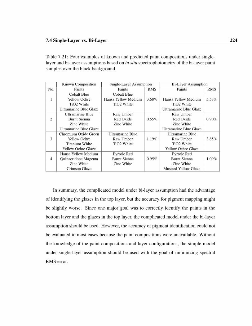
7.4 Single-Layer vs. Bi-Layer 224
Table 7.21: Four examples of known and predicted paint compositions under single-layer and bi-layer assumptions based on in situ spectrophotometry of the bi-layer paintsamples over the black background.
Known Composition Single-Layer Assumption Bi-Layer AssumptionNo. Paints Paints RMS Paints RMS
Cobalt Blue Cobalt Blue1 Yellow Ochre Hansa Yellow Medium 3.68% Hansa Yellow Medium 5.58%
TiO2 White TiO2 White TiO2 WhiteUltramarine Blue Glaze Ultramarine Blue Glaze
Ultramarine Blue Raw Umber Raw Umber2 Burnt Sienna Red Oxide 0.55% Red Oxide 0.90%
Zinc White Zinc White Zinc WhiteUltramarine Blue Glaze Ultramarine Blue GlazeChromium Oxide Green Ultramarine Blue Ultramarine Blue
3 Yellow Ochre Raw Umber 1.19% Raw Umber 3.85%Titanium White TiO2 White TiO2 White
Yellow Ochre Glaze Yellow Ochre GlazeHansa Yellow Medium Pyrrole Red Pyrrole Red
4 Quinacridone Magenta Burnt Sienna 0.95% Burnt Sienna 1.09%Zinc White Zinc White Zinc White
Crimson Glaze Mustard Yellow Glaze
In summary, the complicated model under bi-layer assumption had the advantage
of identifying the glazes in the top layer, but the accuracy for pigment mapping might
be slightly worse. Since one major goal was to correctly identify the paints in the
bottom layer and the glazes in the top layer, the complicated model under the bi-layer
assumption should be used. However, the accuracy of pigment identification could not
be evaluated in most cases because the paint compositions were unavailable. Without
the knowledge of the paint compositions and layer configurations, the simple model
under single-layer assumption should be used with the goal of minimizing spectral
RMS error.

7.4 Single-Layer vs. Bi-Layer 225
Figure 7.8: Measured (red solid line) and predicted reflectance factors under single-layer (blue dashed line) and double-layer (green dash-dotted line) assumptions for fourbi-layer samples over the black background based on in situ spectrophotometry.
7.4.3 Spectral-based Camera
Finally, the single-layer and bi-layer assumptions were tested on reflectance factors
predicted from camera signals for the bi-layer samples over the black background.
Under the complex bi-layer assumtpion, the program successfully identified 75% of
glazes, as listed in Table 7.22. The accuracy of pigment mapping under bi-layer as-
sumption was also slightly worse than that under single-layer assumption (Table 7.23).
The standard derivations for two color difference equations were statistically higher
under bi-layer assumption (Table 7.24).

7.4 Single-Layer vs. Bi-Layer 226
Table 7.22: Accuracy of pigment identification based on reflectance factors predictedfrom spectra-based camera of the bi-layer paint samples over the black backgroundunder single and bi-layer assumptions.
No. of misidentified paints No. of misidentified glazeAssumption 0 1 2 3 Total 0 1single-layer 29 39 42 7 1x39+2x42+3x7 = 144 NA NA
bi-layer 14 75 28 0 1x75+2x28 = 131 88 29
Table 7.23: Statistical results of prediction accuracy based on reflectance factors pre-dicted from spectra-based camera of the bi-layer paint samples over the black back-ground under the single and bi-layer assumptions.
Single-Layer AssumptionMetric Mean Max 95% Percentile Std. Dev.∆Eab 5.63 22.47 14.26 3.75∆E00 3.29 11.02 6.32 1.79
RMS (%) 1.75 5.84 4.65 1.19MI(D65 → A) 0.64 3.12 2.01 0.53
Bi-Layer AssumptionMetric Mean Max 95% Percentile Std. Dev.∆Eab 5.92 31.07 14.45 4.56∆E00 3.81 18.71 9.06 2.94
RMS (%) 1.75 8.57 4.37 1.32MI(D65 → A) 0.66 2.86 1.93 0.55
Table 7.24: Results of statistical tests between the single and bi-layer assumptionsbased on reflectance factors predicted from spectra-based camera of the bi-layer paintsamples over the black background. Symbol “0 means that the null hypothesis that twovalues are the same is accepted at a 95% confidence level, while symbol “1 means thatthe null hypothesis is rejected.
Statistical Test Identification ∆Eab ∆E00 RMS (%) MI(D65 → A)F-test NA 1 1 0 0T-test NA 0 0 0 0

7.4 Single-Layer vs. Bi-Layer 227
Again, four examples were selected with the worst identification of the bottom
layer under the bi-layer assumption. The measured and predicted reflectance factors
are plotted in Figure 7.9. With the exception of the last mixture, the paint compositions
of the bottom layers under the bi-layer assumption was identical to those under the
single-layer assumption (Table 7.25). The RMS errors between those two assumptions
for these four mixtures were also similar. Since all four examples had low reflectance
values (Figure 7.9), the RMS errors were pretty small. It was also noted that the pro-
gram could not correctly identify the glazes in top layer because of the wrong pigment
identification for the bottom layer.
Table 7.25: Four examples of the known and predicted paint compositions undersingle-layer and bi-layer assumptions based on spectral-based camera of the bi-layerpaint samples over the black background.
Known Composition Single-Layer Assumption Bi-Layer AssumptionNo. Paints Paints RMS Paints RMS
Ultramarine Blue Diarylide Yellow Diarylide Yellow1 Yellow Ochre Green Gold 1.10% Green Gold 0.98%
Zinc White Zinc WhiteMustard Yellow Glaze Ultramarine Blue Glaze
Ultramarine Blue Raw Umber Raw Umber2 Hansa Yellow Medium Green Gold 0.68% Green Gold 0.72%
Zinc White Zinc WhiteMustard Yellow Glaze Ultramarine Blue Glaze
Cobalt Blue Dairylide Yellow Diarylide Yellow3 Burnt Sienna Quinacridone Magenta 1.12% Quinacridone Magenta 0.76%
Zinc White Zinc WhiteCrimson Glaze Ultramarine Blue Glaze
Ultramarine Blue Phthalo Green Phthalo Green4 Quinacridone Magenta Pyrrole Red 0.70% Pyrrole Red 0.73%
Cobalt BlueCrimson Glaze Ultramarine Blue Glaze
To sum it up, the complicated model under bi-layer assumption had the advantage

7.5 Conclusions 228
Figure 7.9: Measured (red solid line) and predicted reflectance factors under single-layer (blue dashed line) and double-layer (green dash-dotted line) assumptions for fourbi-layer samples over the black background based on spectral-based camera.
of identifying the glazes in the top layer with 75% chance of success, and the accu-
racy for pigment mapping was slightly worsen than that under the simple single-layer
assumption.
7.5 Conclusions
In this chapter, whether knowledge of opacity and layer configuration were useful to
improve prediction accuracy had been investigated with both in situ spectrophotometry
and spectra-based camera. The opaque vs. translucent and single vs. bi-layer assump-
tions were compared based on the accuracies of pigment identification and pigment
mapping. Some conclusions are summarized in Table 7.26.

7.5 Conclusions 229
Table 7.26: Comparison results for opaque vs. translucent and single vs. bi-layerassumptions based upon both in situ spectrophotometry and spectra-based camera.
Sample Type Measurement CommentsFilms over in situ Translucent assumption was slightly superior
white spectrophotometry to opaque one.Films over in situ Translucent assumption was significantly
black spectrophotometry better than opaque one.Bi-layer films in situ Bi-layer assumption was slightly better than
over black spectrophotometry single-layer one, and identified the glazesin the top layer with 85% success rate.
Films over spectral-based Difference between opaque and translucentwhite Camera was negligible.
Bi-layer films Spectral-based Difference between single and bi-layerBlack Camera was negligible, and bi-layer assumption
identified the glazes with 75% success rate.
With a prior knowledge of constituent pigments and layer configuration, the accu-
racy of pigment mapping was analyzed independently from the accuracy of pigment
identification. The opaque and translucent assumptions were tested on the single-layer
samples over both white and black backgrounds. The effect of black (or white) back-
ground was equivalent to adding black (or white) paint in the translucent paint sam-
ples. If both black and white paints as extra components were incorporated into the
pigment-mixing model for the opaque case, these two assumptions were not signifi-
cantly different with respect to the accuracy of pigment mapping. The concentration
precision of 5% for other paints was sufficient, while black paint was very sensitive to
the variation of concentration (0.1%). The current exhaustive search method searched
the best concentrations for a pigment composition with the precision of 5%, so a new
routine to optimize the concentrations was required. The single-layer and bi-layer as-
sumptions were tested on the bi-layer samples over the black background. Under the
single-layer assumption, the glaze layer was totally discarded, and only the constituent

7.5 Conclusions 230
pigments in the bottom layer were used to estimate the reflectance factor of the bi-
layer paint sample. Under the bi-layer assumption, the constituent pigments in the
bottom layer and glazes in the top layer were known. Both the pigment concentrations
and the thickness of the glaze layer were optimzied. Both colorimetric and spectral
accuracies under the bi-layer assumption were significantly better than those for the
single-layer assumption. Thus, the bi-layer assumption was significantly superior to
the single-layer assumption when constituent pigments and glaze were known.
In order to do pigment mapping under translucent assumption, the absorption and
scattering coefficients for each and every paint in the database were required to be
characterized on an absolute basis, and the paint samples should be carefully prepared
on an opacity paper with controlled thickness. Since reflectance factors were non-
linearly related to pigment concentrations, the mixing model was nonlinear with the
goal of minimizing the spectral RMS error. The computation time of reflectance factor
from the absorption and scattering coefficients of the mixture sample under translucent
assumption (general form of K-M theory) was doubled when compared with opaque
assumption (simplified form of K-M theory). Also, the background reflectance factor
should be able to be estimated. The bi-layer assumption had even stricter requirements.
Both paints in the bottom layer and glazes in the top layer should be characterized on
an absolute basis. The thicknesses of both layers should be able to estimated.
Because of the inaccuracy of the pigments’ optical properties as functions of thick-
ness, imprecision of reflectance measurement and imperfectness of the K-M theory, the
knowledge of opacity and layer-configuration was slightly beneficial to improve the ac-
curacies of both pigment identification and mapping. Incorporating the inaccuracy of
the camera system, the advantage of the knowing opacity and layer configuration was
even less pronounced. For paintings, it is impossible to know the paint composition

7.5 Conclusions 231
for each pixel, so the correctness of pigment identification and accuracy of concen-
tration prediction cannot be done pixel-wise. The possible error metrics for paintings
were colorimetric and spectral accuracies of predicted reflectance factors from both
camera signals and pigment maps. So for paintings, the simple opaque model under
single-layer assumption should be used to do pigment mapping with the objective of
minimizing spectral RMS error.
The method of pigment mapping was exhaustive search with the objective func-
tion of minimizing the spectral RMS error. Except for the over-fitting mentioned in
the introduction section, there were several issues needing to be addressed. The con-
centration precision of 5% was sufficient for other paints except for black paint. The
thickness precision of the glaze layer might not be sufficient. Also, it was possible that
two reflectance spectra were very close but had quite different paint compositions. The
accuracy of the pigment-mixing model with a prior knowledge of constituent pigments
and layer configuration was limited. Thus, the program had some trouble in identifying
the right paint compositions for some mixtures.

Chapter 8
Case Studies of Two Paintings
“I have a larger picture of the village church an effect in which the building appears to
be violet-hued against a sky of simple deep blue colour, pure cobalt; the stained-glass
windows appear as ultramarine blotches, the roof is violet and partly orange. In the
foreground some green plants in bloom, and sand with the pink flow of sunshine in
it. And once again it is nearly the same thing as the studies I did in Nuenen of the
old tower and the cemetery, only it is probably that now the colour is more expressive,
more sumptuous.”
- Abridged from Letter from Vincent van Gogh to Wilhelmina van Gogh, Auvers-
sur-Oise, 5 June 1890 (http://webexhibits.org/vangogh/letter/21/W22.htm)

8.1 Introduction 233
8.1 Introduction
In this chapter, spectral imaging and pigment mapping were applied to two paintings.
One painting was painted by a local artist Bernard Lehmann and named as Auvers
since it was a copy of Vincent van Gogh’s The Church at Auvers, shown in Figure 8.1.
The other painting, The Starry Night was painted by Vincent van Gogh in 1889, shown
in Figure 8.2. It is in the permanent collection of the Museum of Modern Art in New
York City. The oil paints used in this famous painting have not been determined. After
exhibition for more than one hundred years, some paints might have been faded, and
the canvas was noticeably aged. Therefore, the pigment mapping for The Starry Night
was much more challenging.
(a) Vincent van Gogh The Church at Auvers (b) Bernard Lehmann Auvers
Figure 8.1: (a) Vincent van Gogh The Church in Auvers-sur-Oise, View from Chevet,1890 (Digital image courtesy of the Trustees of Musee d’Orsay, Paris (b) the sRGBrepresentation of Bernard Lehmann Auvers.

8.1 Introduction 234
Figure 8.2: The sRGB representation of Vincent van Gogh The Starry Night, 1889.
The Sinar camera coupled with two optimized filters was used to image these two
paintings. This camera system achieved high colorimetric and spectral accuracies. The
matrix R method, discussed in Chapter 3, was used to build the transformation and con-
vert the camera signals to spectral reflectance factor. The painting Auvers was captured
in the lab at RIT. The paints used were Golden matte fluid acrylic paints and acrylic
color glazes, which had been characterized on an absolute basis with the two-region
method (Chapter 6). The painting surface was uneven, and visual inspection revealed
that both opaque and translucent regions existed. According to the artist, two colored
glazes were also used later. Ideally, the general translucent model for multiple-layer
configuration should be assumed. However, it was concluded from the previous chap-
ter that the opacity and layer-configuration were not critical to both spectral and col-
orimetric accuracies of pigment mapping. So pigment mapping for Auvers was based
upon the two-constant Kubelka-Munk (K-M) theory under the opaque and single-layer

8.2 General Procedure of Pigment Mapping 235
assumptions.
The unframed The Starry Night was imaged in the conservation studio of the Mu-
seum of Modern Art. The dimensions of the painting are 28.75” by 36.25”. In or-
der to achieve the highest spatial resolution, the image almost filled the entire image
plane. Twenty spots on the painting were selected by experts and measured with a
bi-directional spectrophotometer X-Rite Eye-One. The location of each spot on The
Starry Night was measured and recorded. These twenty measurements were used as the
only ground-truth data for both camera prediction and pigment mapping. The paints
used in the painting were unknown. The palette was approximated using six oil pig-
ments selected from the Gamblin conservation colors and four additional colors based
on historical knowledge of van Gogh’s working method. The pigment mapping was
based on the single-constant K-M theory for the opaque case.
The general procedure of pigment mapping will be introduced first. Since these
two paintings differ in the database and theory used for pigment mapping, they will
be addressed separately. For each painting, the discussion will include spectral-based
camera, pigment mapping for a limited number of measurement spots, pigment map-
ping for the entire image, and possible future applications. Finally, the conclusions
based on these two case studies will be drawn.
8.2 General Procedure of Pigment Mapping
The reconstruction of spectral reflectance from camera responses was discussed in
Chapter 3, and will not be reiterated here. The main focus is to map a painting’s
constituent pigments and concentrations. It is practically difficult to perform pigment
mapping on pure pixel-basis without considering similarity among neighboring pixels,

8.2 General Procedure of Pigment Mapping 236
due to issues like computation time and data storage. For example, the sensor resolu-
tion of Sinar camera is 5440 × 4080 pixels. If the number of wavelength is 31 (from
400nm to 700nm, at 10nm interval), the size of a spectral image is about 1.28GB.
Most programs cannot handle such a big file, and the general practice is to divide the
large image into several small images either spatially or spectrally. On the other hand,
if the process time of pigment mapping for each pixel using the method of exhaustive
search is 0.5 second, the total time for processing the entire Sinar image is roughly 128
days, which is obviously unacceptable.
Different approaches should be used. Although the number of pixels in a image
is huge, the number of possible paint combinations is limited. For example, given
10 paints in the database, if the number of paints in each pixel is limited to three, the
number of possible paint combinations is C110+C2
10+C310 = 175. The number of actual
paint combinations used in the painting is even less. Ideally, the image is segmented
into several clusters, and for each cluster, only one paint combination exists. Such
image segmentation is very difficult to achieve. One practical approach was discussed
in Chapter 4. The image was first segmented based on chromatic information, and for
each cluster, no more than four paints were selected to perform pigment mapping pixel-
wise. If the pigment concentration calculated was less than a predefined threshold
(e.g., 1%), the corresponding pigment was eliminated. The computation efficiency
was greatly improved by focusing on a subgroup of pigments rather than unmixing
with the entire pigment database for each pixel. For a even larger image, a more
practical approach should be used. The pigment mapping was only performed on a
limited number of pixels, and the pigment composition of each pixel of interest was
assigned with that of those limited pixels based on similarity calculation between the
pixel of interest and those pixels. The big assumption of this new approach was that

8.2 General Procedure of Pigment Mapping 237
the selected limited pixels should be representative of all the pixels in the painting. An
obvious side-effect of this approach was the error or noise in the pigment maps, which
was very similar to quantization error. The only way to alleviate the side-effect was to
increase the number of the selected pixels to perform pigment mapping, which in turn
increase the total computation time.
The new proposed method is introduced next. The schematic flowchart of this
method is plotted in Figure 8.3. This method takes advantage of both image segmen-
tation and similarity among pixels, and also considers the balance among computation
time, resolution and accuracy. First, the large image is divided into several small im-
ages, spatially. All the processes described below will be repeated for each small
image. Second, the small image is grouped into several clusters based on supervised
image classification. Third, a large number of pixels is selected by uniformly sampling
in CIELAB space. Camera signals for these pixels are extracted and transformed to
spectral reflectance factors, and then paint compositions for these pixels are calculated
from the pigment mapping program. Next, camera signals that belongs to the first
cluster are extracted and compared with camera signals of these selected pixels. The
similarity metric is the simple Euclidean distance between camera signals. The paint
composition of the selected pixel that is closest to the pixel of interest will be the paint
composition of that pixel. The process is repeated for each pixel and then for each
cluster. Then the pigment map of each paint is constructed by stitching all the small
pigment maps together. Finally, the ICCLAB image can be rendered from these pig-
ment maps along with the optical properties of these paints for a certain combination of
illuminant and observer. With pigment maps, other useful applications can be done as
well. For example, the color appearance of the painting can be simulated if the optical
property of one paint is replaced by that of another.

8.2 General Procedure of Pigment Mapping 238
1. I
mag
e Par
tition
4. P
igm
ent
Map
pin
g fo
r Im
age
Bas
ed o
n S
imila
rity
Cla
ssifi
ed Im
age
N S
pots
4.1
Sel
ecte
d n
Spots
fo
r th
e i-th
Cla
ss
Cam
era
Imag
es
+ +
4.2
Seg
men
ted
i-th
Cla
ss
4.3
Sim
ilari
tyC
alcu
lation
&
Com
par
ison
4.4
Pig
men
t M
aps
P1
Pk
P2
..
.
3. P
igm
ent
Map
pin
g fo
r N
Spots
3.1
Extr
act
Cam
era
Res
ponse
sR
etri
eve
Refl
ecta
nce
for
N s
pots
N s
pots
Cam
era
Imag
esPig
men
t D
atab
ase
Pig
men
t U
nm
ixin
g A
lgori
thm
3.2
Obta
in b
oth
Pai
nts
and
Conce
ntr
atio
ns
for
N S
pots
2. I
mag
e C
lass
ifica
tion
2.1
Sel
ect T
rain
ing
Reg
ions
bas
ed o
n s
RG
B Im
age
sRG
B Im
age
Trai
nin
g R
egio
ns
2.2
Cla
ssifi
cation b
ased
on
two c
amer
a im
ages
Cam
era
Imag
esC
lass
ified
Im
age
1. I
mag
e Par
tition
2. I
mag
e C
lass
ifica
tion
3. P
igm
ent
Map
pin
g fo
r N
Spots
4. P
igm
ent
Map
pin
g fo
r Im
age
5. I
mag
eC
om
bin
atio
n6. I
mag
eR
ender
ing
5. I
mag
e C
om
bin
atio
n6. I
mag
e R
ender
ing
Figure 8.3: Schematic flowchart of pigment mapping of paintings.
8.2 General Procedure of Pigment Mapping 239
8.2.1 Image Partition
First, the large image was segmented into several small images depending on the num-
ber of pixels in the large image and the capacity of computer memory. Each small
image was mapped separately. For each target, there are four types of images to be
partitioned: two camera images, one sRGB image and one ICCLAB image rendered
from camera signals. The usage of these image types is as follows:
1. The sRGB image was used for display purposes and to facilitate selecting the
training regions for supervised image classification.
2. The two camera images were used to form the six-channel camera responses and
to reconstruct spectral reflectance factors. Both camera responses and reflectance
factor for each pixel were obtained during the process. So it was not necessary
to save the large spectral image.
3. The ICCLAB image was used later to compare with the ICCLAB image rendered
from pigment maps. Since paint composition information for each pixel was
unavailable, it was impossible to evaluate the accuracy of pigment identification
and pigment concentration. One possible way to evaluate the performance of
pigment mapping was to compare the rendered image from pigment maps with
that rendered from camera signals. The two rendered images were displayed
side-by-side on a calibrated monitor and compared visually.
8.2.2 Image Classification
For each small image, some training regions were selected manually and assigned
with particular group numbers. The number of groups was determined based on the

8.2 General Procedure of Pigment Mapping 240
colorimetric information and operator experience. The selection of training regions is
the only manual step in this newly proposed method. The simple linear classifier was
used (Duda et al., 2001). For the two-group case, the linear classifier assumed that
the probability density functions of the two groups are both normally distributed and
their covariance matrices are identical. Under these assumptions, the Bayes optimal
solution was used to predict each observation x as being from the second group based
on a linear discrimination function, as defined in Eq. (8.1). The function became a
threshold on the dot product between the weighting vector w and the observation x for
some constant c. The weighting vector was related to the covariance matrix Σ and the
mean vectors, µ1 and µ2, of two groups [Eq. (8.2)]. For more than two groups, more
than one discrimination function [Eq.(8.1)] were estimated. If the number of groups
was k, the number of discrimination functions was k(k − 1)/2.
w · x < c (8.1)
w = Σ−1 (µ2 − µ1) (8.2)
For example, the small image of the moon, shown in Figure 8.4, was classified
into five groups: orange moon, yellow cloud surrounding the moon, blue-green cloud
further outside the moon, dark blue sky and aged canvas. The training regions of
these groups are shown in Figure 8.5(a). Except for the blue-green cloud, one training
region was selected for each class. Due to the small spatial areas of blue-green cloud,
two small regions were selected.
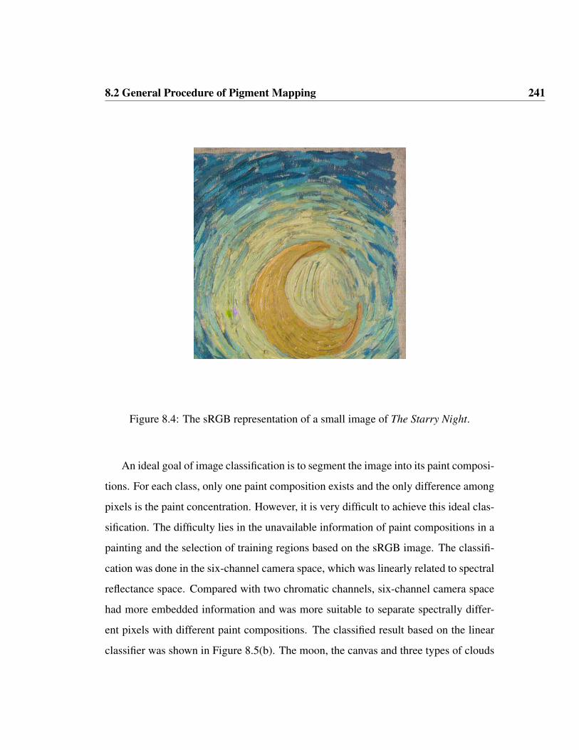
8.2 General Procedure of Pigment Mapping 241
Figure 8.4: The sRGB representation of a small image of The Starry Night.
An ideal goal of image classification is to segment the image into its paint composi-
tions. For each class, only one paint composition exists and the only difference among
pixels is the paint concentration. However, it is very difficult to achieve this ideal clas-
sification. The difficulty lies in the unavailable information of paint compositions in a
painting and the selection of training regions based on the sRGB image. The classifi-
cation was done in the six-channel camera space, which was linearly related to spectral
reflectance space. Compared with two chromatic channels, six-channel camera space
had more embedded information and was more suitable to separate spectrally differ-
ent pixels with different paint compositions. The classified result based on the linear
classifier was shown in Figure 8.5(b). The moon, the canvas and three types of clouds

8.2 General Procedure of Pigment Mapping 242
(yellow, blue-green and dark blue) were separated clearly. The classification was very
satisfactory.
(a) Training Regions (b) Classified Image
Figure 8.5: (a) Five training regions (1. light blue: orange moon 2. lime blue: yellowcloud 3. yellow: blue-green cloud 4. orange: blue sky 5. red: darkened canvas). (b)The classified image using the linear discrimination function.
The above classification algorithm required the training data supplied based upon
the observer’s experience, so it belonged to a supervised algorithm. The K-Means
unsupervised classification discussed in Chapter 4 was not used for several reasons.
The unsupervised K-Means algorithm iteratively updated the center of each group until
the change was negligible, so the algorithm was quite slow. Furthermore, the K-Means
algorithm was sensitive to the selection of initial centers and might not converge. The
K-Means algorithm was also applied to classify the moon image (Figure 8.4) based on
six-channel camera signals and two chromatic channels (a∗, b∗). The classified results
are shown in Figure 8.6. The size of the moon image was 480 × 482 pixels. The
running times on a PowerBook G4 for the above supervised method and the K-Means

8.2 General Procedure of Pigment Mapping 243
algorithm in two different spaces were 6s, 207s and 68s, respectively. The supervised
method was the fastest and the most efficient. The result [Figure 8.6(a)] using the
K-Means algorithm in six-channel camera space was unsatisfactory. The moon and
canvas were classified into the same group, and also three types of clouds were mixed
in some places. The classification result [Figure 8.6(b)] using the K-Means algorithm
in two chromatic channels was closer to the result [Figure 8.5(b)] for the supervised
classification. There were lots of isolated points in Figure 8.6(b). For example, there
were plenty of lime blue dots and red dots in the moon region. The classification
results of the K-Means algorithm were obviously worse than that for the supervised
algorithm. So the supervised algorithm was used to perform image segmentation.
(a) Six-channel camera signals (b) Two chromatic channels (a∗,b∗)
Figure 8.6: The classified images using the unsupervised k-means algorithm based onsix-channel camera signals (a) and two chromatic channels (a∗,b∗).
8.2 General Procedure of Pigment Mapping 244
8.2.3 Pigment Mapping for a Limited Number of Pixels
The pigment mapping was based on K-M theory. The program, using an exhaustive
search method, was written in the C language. Depending on the number of candidate
paints in the database, the concentration precision (e.g., 5%), and the model selection
(opaque or translucent), the running time varied drastically from milliseconds to sev-
eral seconds. For example, if the number of paints was 12, the concentration precision
was 5%, and the model was the two-constant K-M theory under the opaque assump-
tion, the running time per pixel was about 0.5 second on a Power Mac G5. The total
processing time for 1000 pixels was about 10 min, which was tolerable.
For each small image, about 1000 circular spots were selected by uniformly sam-
pling in CIELAB space. Each spot included 13 pixels surrounding each position, as
shown in Figure 8.7. The camera signals of these 13 pixels were averaged to represent
each spot in order to reduce noise. The circular spot was chosen to simulate the aper-
ture of a spectrophotometer. First, the 16 bits ICCLAB image was transformed to a
8-bit CIELAB image. Then these CIELAB values were sorted, and the redundant val-
ues were removed. The down-sampling rate was then calculated based on the number
of CIELAB values in the small image and the number of the spots (1000). The posi-
tion of each selected CIELAB values was recorded. The mask image of about 1000
spots was a black-white image where the background was set to zero and each spot
was assigned with the same number.

8.2 General Procedure of Pigment Mapping 245
Figure 8.7: A circle 5x5 mask image.
After the mask image was built, the camera signals for these spots were extracted
from the two camera images, and then averaged over each spot. The reflectance factors
were calculated from these averaged camera signals using the matrix R method, dis-
cussed in Chapter 3. The optical properties, the absorption and scattering coefficients
for each paint in the database, were available. The paint compositions were calculated
from the reflectance factors using the exhaustive search routine written in the C lan-
guage. The averaged camera signals and paint compositions for each spot were saved
and used in the next section.
8.2.4 Pigment Mapping for an Image Based on Similarity
Each small image was classified into several clusters. The camera signals were ex-
tracted for the first cluster, and the pre-mapped spots that belonged to this cluster were
also extracted. The similarity metric was the simple Euclidean distance in six-channel
camera space: the smaller the metric, the more similar. The distances between each
pixel in this cluster and all these pre-mapped spots were calculated. The paint com-
position of the spot that was the most similar to the pixel of interest was assigned to

8.2 General Procedure of Pigment Mapping 246
that pixel. The whole process was repeated for all the pixels in this cluster and then for
the next cluster until all the clusters were proceed. The output was a series of pigment
maps for each small image.
8.2.5 Image Combination
After the pigment maps for all small images were generated, it was very easy to stitch
them together into a large image for each pigment.
8.2.6 Image Rendering
Finally, the ICCLAB image was rendered from the pigment maps and optical proper-
ties of these pigments for the same illuminant and observer as the image rendered by
spectral-based camera. These two rendered images can be displayed side-by-side on
a calibrated monitor. Visual inspection was used to evaluate the colorimetric accuracy
of pigment mapping.
Other useful applications can also be done with these pigment maps. For example,
if the change of optical property of a paint with the exposure time can be modeled,
the color appearance of the painting can be simulated as the paint is gradually faded.
It is also possible to replace one paint by the other, and to predict the change in the
color appearance of the painting. Another possible application is to aid conservators
for retouching the damaged areas in paintings. In summary, these pigment maps will
provide valuable knowledge of the painting, and can be used for color appearance
simulation and digital rejuvenation.

8.3 Lehmann’s Auvers 247
8.3 Lehmann’s Auvers
This painting was painted by the artist Bernard Lehmann, and named as Auvers by
the artist, since it was a copy of the famous masterpiece of van Gogh’s The Church at
Auvers. The two original paintings The Church at Auvers and The Starry Night were
pained by Vincent van Gogh in 1890 and 1889, respectively. There were large areas
of blue sky in both paintings. Vincent van Gogh used both cobalt blue and ultrama-
rine blue in The Starry Night, based on contact spectrophotometric measurements of
the painting. Coincidentally, Lehmann also used both blue pigments in his painting:
ultramarine blue used for the blue sky and cobalt blue for the window, based on re-
sults of pigment mapping. These two blue pigments have their unique reflectance in
longer wavelengths and change color differently according to variation of lighting in
this region. Thus, Auvers was a very good study target. If it can be rendered with
high colorimetric accuracy on a monitor or in print, it will provide more confidence to
reproduce the masterpiece of Vincent van Gogh.
For Auvers, the paints used were Golden matte fluid acrylic paints and color glazes.
Knowledge of the paints comprising the painting was critical for pigment mapping.
Since information on paints used in The Starry Night was not available, the first and
the most difficult step of pigment mapping was to find the proper paints to form van
Gogh’s palette. The paints used in Auvers were characterized on an absolute basis
using the two-region method described in Chapter 6. Close visual inspection showed
that most parts were totally opaque, and only the sand road in the middle bottom of
painting might be translucent. According to the artist, ultramarine blue glaze was used
to darken the orange roof, and yellow glaze was also used in some parts of the painting.
There were equivalent blue and yellow paints spectrally similar to the blue and yellow
glazes, so it was very hard to distinguish these color paints from glazes. It was also

8.3 Lehmann’s Auvers 248
concluded from the previous chapter that the opacity and layer configuration were
not significantly beneficial to pigment mapping when using a spectra-based camera.
So the two-constant K-M theory under the opaque and single-layer assumptions were
used when pigment mapping of Auvers.
The accuracy of the camera prediction is discussed first. Thirty spots were marked
on Auvers and measured with a bi-directional spectrophotometer. These thirty spots
were used to examine the spectral accuracy of the camera system. After that, the pig-
ment mapping was implemented on these spots. The accuracies of pigment mapping
for these spots based on both contact spectrophotometric measurements and reflectance
factors predicted from the camera system were evaluated. Finally, the pigment map-
ping will be done on the entire image using the general procedure described in the
previous section. The CIELAB image was reconstructed from these pigment maps
and optical properties of these pigments. The validity of these pigment maps will be
evaluated through soft proof of the reconstructed CIELAB image.
8.3.1 Spectral-Based Camera
The camera system was a traditional Color-Filter-Array (CFA) camera coupled with
two optimized filters, a yellow filter and a blue filter. Two tungsten light sources were
placed 45o on either side of the optical path. Because of the lower power of tungsten
light at shorter-wavelengths, the signal for blue channel was low even with an exposure
setting that almost saturated the red channel. For each light source, a blue filter was
installed in the front of the light bulb, and covered by the softbox. The relative power
distributions of light source with and without the blue filter are plotted in Figure 8.8.
The CCT for the light source with the blue filter was about 5485K, while the CCT for
the original light source was close to 2800K. It was obvious that the distribution of light

8.3 Lehmann’s Auvers 249
source with the blue filter was more flat below 680nm, so the three-channel exposures
were more balanced. Optimal exposure time was chosen based on trial and error for
each filter, and they were 11.6
s and 1.6s for the yellow and blue filters, respectively.
Figure 8.8: Spectral power distributions of light source with and without the blue filter.
There were four targets: ColorChecker DC (abbreviated as CCDC), the ESSER
TE221 scanner target (ESSER) and two targets made up of Golden acrylic paints. One
target had 78 big-square patches (Big-Square). There were 14 chromatic paints, 4
glazes and two white paints in total. For each chromatic paint or glaze, there were
four patches (one masstone sample and one mixture sample with zinc white over both
a white and a black background). For each white paint, there were two patches (one
masstone sample over both backgrounds). In addition, there were two patches for both
white and black backgrounds of a contrast paper. So the total number of patches for
Big-Squares was 18 × 4 + 2 × 2 + 2 = 78. The other had 234 small square patches
(Small-Square). Half of patches in the Small-Square target were single-layer paint
films over the white background of contrast paper, and the other half were bi-layer
paint films over the black background. This target had been used to test whether the

8.3 Lehmann’s Auvers 250
opacity and layer configuration were critical to pigment mapping for the spectral-based
camera in the previous chapter. The accuracy of camera prediction for this target is
discussed next.
These four targets could all be used as the calibration target to build the transfor-
mation matrix of the camera system. Because the two Golden targets lack gray patches
and spectral variability, either one was not suitable as the calibration target alone, but
might be used together with either CCDC or ESSER. It is known that CCDC cannot
predict the long-tail of cobalt blue from the previous experiment (Chapter 3). Since
cobalt blue was used in the two Golden targets and the painting Auvers, it was benefi-
cial to combine one of the Golden targets with either CCDC or ESSER. The choice of
calibration targets were CCDC, ESSER, CCDC plus Big-Square, CCDC plus Small-
Square, ESSER plus Big-Square, and ESSER plus Small-Square. It is well-known that
human visual system is very sensitive to gray colors. There were 76 gray patches in
CCDC, while only 19 gray patches were in ESSER. There are two ways to effectively
increase the number of gray patches for ESSER: one was to weight these 19 gray
patches more than the other colored patches in the objective function, and the other
was to repeat the gray patches multiple times in deriving the transformation matrix.
The later method was chosen, and the gray patches were replicated seven times. Then
the total number of patches for ESSER was 264 + 19 × 7 = 397 (264 color patches).
After that, the ratio of gray patches to color patches for ESSER was 19×7264
= 0.50,
comparable to the ratio for CCDC ( 76240−76
= 0.46). Both spectral and colorimetric ac-
curacies were compared when the camera system was characterized with the different
calibration targets.
The statistical results of both spectral RMS (%) error and color difference ∆E00
for the verification targets when the camera system was characterized with different

8.3 Lehmann’s Auvers 251
calibration targets are listed in Tables 8.1 and 8.2. It was expected that both spectral
and colorimetric accuracies of a verification target were higher if this target was also
used as the calibration target. Both metrics vary slightly among the different calibration
targets.
Table 8.1: Statistical results of spectral RMS (%) error of each verification target whenthe camera system was characterized with the different calibration targets.
Calibration Target Verification TargetsName No. Statistics CCDC ESSER Big-Square Small-Square All TargetsCCDC 240 Mean 1.37 1.66 2.66 2.30 1.83
Std. Dev. 0.63 0.90 2.12 1.57 1.26ESSER 397 Mean 1.68 1.39 2.58 1.87 1.68
Std. Dev. 0.95 0.76 1.86 1.11 1.08CCDC & 320 Mean 1.47 1.63 2.31 1.93 1.72
Big-Square Std. Dev. 0.62 0.86 1.75 1.18 1.03CCDC & 474 Mean 1.49 1.64 2.47 1.65 1.68
Small-Square Std. Dev. 0.63 0.79 2.00 0.87 0.97ESSER & 477 Mean 1.69 1.41 2.31 1.76 1.64
Big-Square Std. Dev. 1.00 0.81 1.65 1.02 1.03ESSER & 631 Mean 1.69 1.42 2.44 1.65 1.63
Small-Square Std. Dev. 0.97 0.80 1.81 0.85 1.01

8.3 Lehmann’s Auvers 252
Table 8.2: Statistical results of color difference ∆E00 error of each verification targetwhen the camera system was characterized with the different calibration targets.
Calibration Target Verification TargetsName No. Statistics CCDC ESSER Big-Square Small-Square All TargetsCCDC 240 Mean 0.79 1.12 1.44 1.96 1.27
Std. Dev. 0.56 0.77 1.22 1.40 1.06ESSER 397 Mean 1.09 0.78 1.42 2.15 1.25
Std. Dev. 0.90 0.55 1.00 1.66 1.18CCDC & 320 Mean 0.81 0.99 1.12 1.50 1.08
Big-Square Std. Dev. 0.59 0.60 0.71 0.69 0.68CCDC & 474 Mean 0.86 1.15 1.24 1.23 1.10
Small-Square Std. Dev. 0.65 1.06 0.97 0.61 0.88ESSER & 477 Mean 0.98 0.81 1.11 1.52 1.05
Big-Square Std. Dev. 0.76 0.61 0.63 0.94 0.80ESSER & 631 Mean 0.98 0.84 1.16 1.22 0.99
Small-Square Std. Dev. 0.66 0.58 0.65 0.60 0.63
Statistical tests were used to evaluate which calibration target was significantly
better with respect to spectral and colorimetric accuracies when all the targets were
used as the verification target (the last columns in Tables 8.1 and 8.2). The statis-
tical F-test tested whether the standard derivations of two groups were significantly
different, while the student T-test tested whether the means of two groups were dif-
ferent. The CCDC when used as the calibration target was compared with the other
choices of the calibration target. The color difference for CCDC as the calibration
target was statistically worse than that for all the other choices, and the spectral RMS
error for CCDC as the calibration target was only statistically worse than that for the
ESSER+Small-Square as the calibration target. Furthermore, the CCDC+Big-Squares
was compared with ESSER+Small-Squares used as the calibration target. These two
choices of the calibration targets were not significantly different. There were only 320
patches for CCDC+Big-Squares, while 631 patches for ESSER+Small-Squares. Fi-
nally, CCDC+Big-Square was used as the calibration target to build the transformation

8.3 Lehmann’s Auvers 253
matrix of the camera system. The mean color difference was about 1 ∆E00 for all the
targets used as verification target, and the mean RMS error was about 1.7%. Both the
colorimetric and spectral accuracies of the camera system calibrated with CCDC+Big-
Square were sufficient enough for pigment mapping.
Next, the transformation matrix was applied on the two camera images of Auvers.
There were 30 marked spots on Auvers, as shown in Figure 8.9. A mask file of these
30 spots was also built, and each spot was approximately the same size as the aperture
size of the spectrophotometer. The camera signals were extracted for these spots and
then averaged. The reflectance factors for these spots were calculated from the aver-
aged camera signals using the transformation matrix derived earlier. So the measured
reflectance factors with the spectrophotometer were compared with the calculated re-
flectance factors from the camera signals.

8.3 Lehmann’s Auvers 254
Figure 8.9: The sRGB representation of the reconstructed multispectral image of thepainting Auvers painted by Bernard Lehmann with 30 marked spots.
The measured and calculated spectral reflectance factors from camera signals are
plotted in Figure 8.10. It was seen that predicted reflectance spectra were very similar
to measurements. The second patch (No. 22) on the fifth row was an exception, and
two spectral curves have noticeable difference in the longer wavelengths. Measure-
ments Nos. 16 and 22 had very similar colors, revealed by visual inspection of the

8.3 Lehmann’s Auvers 255
painting, but measured reflectance for No. 22 was apparently lower than that for No.
16. There are several black strips close to No. 22. So the discrepancy between mea-
sured and predicted reflectance factors for No. 22 might be caused by the difference in
spot position measured by the spectrophotometer and the camera. Another noticeable
difference was observed for the fourth patch on the second row (No. 9). The measured
reflectance for No. 9 had a stair-like shape in the middle of the visible range, while the
predicted curve was much smoother in that region. The pigment mapping for No. 9
based on predicted reflectance was more challenging because the unique characteristic
(stair-like shape) was lost. This spot will be mentioned again in the next section.
Figure 8.10: Measured (red line) and predicted (blue line) reflectance factors fromcamera signals for 30 spots in the painting Auvers.

8.3 Lehmann’s Auvers 256
The statistical results of both spectral and colorimetric error metrics between mea-
sured and predicted reflectance factors are listed in Table 8.3. The mean and standard
derivation of spectral RMS error for these spots were comparable to those of the cali-
bration target of Big-Square, listed in Table 8.1, while the mean and standard deriva-
tion of color difference ∆E00 were slightly worse. The lower color accuracy might be
caused by many dark spots that were selected and marked in Auvers. For these dark
colors, the spectral RMS error was negligible, but the color difference was noticeable.
Overall, the spectral accuracy of camera was sufficient enough to perform pigment
mapping, which will be discussed in the next section.
Table 8.3: The statistical results of both spectral and colorimetric error metrics betweenmeasured and predicted reflectance factors from camera signals for 30 marked spots ofthe painting Auvers.
Statistics Mean Max 95Percentile Std. Dev.∆Eab 3.21 11.41 7.88 2.43∆E00 2.42 11.43 8.31 2.38
RMS(%) 2.31 9.18 4.26 1.59MI D65 → A 0.82 6.55 4.68 1.39
8.3.2 Pigment Mapping
The dimensions of Auvers were 16 inch by 20 inch, and the image size was 1304 pixels
by 1638 pixels. The physical size of each pixel was 0.3 mm by 0.3 mm, which was
far smaller than the size of single brush stroke. So it was impossible that there were
more than one mixture in each pixel. Unlike hyper-spectral images taken from the
air, in which a pixel might combine different materials (e.g., grass and soil), only one
optically-mixed paint mixture could exist in each pixel of Auvers. This is one important
assumption that the pigment mixing model was based on.

8.3 Lehmann’s Auvers 257
The image was divided into 9 small images. Each small image size was about 435
pixels by 546 pixels. The total number of pixels was 237,510. If the running time for
pigment mapping of 1000 pixels was about 10 min, the pigment mapping for this small
image was about 40 hours. The pigment mapping program was an exhaustive search
method written in the C program. As mentioned earlier, two other methods - modi-
fied statistical method and nonlinear forward stepwise regression - were even slower
because they called the MATLAB optimization function multiple times. However, for
this practical procedure, the image spatial resolution was sacrificed to some extent by
selecting only 1000 spots to do pigment mapping and mapping other pixels based on
similarity with these 1000 spots.
First, the accuracy of the pigment mapping program was tested with spectropho-
tometric measurements of 30 marked spots in Auvers (Figure 8.9). Then, the program
was tested with reflectance factors predicted from the camera signals. Next, the pig-
ment mapping was performed for each cluster and then for each small image. After
that, concentration maps for each pigment from all the small images were combined
into a complete map for the entire image. The performance of pigment maps was eval-
uated through both soft proof and hard proof. The ICCLAB image was rendered from
pigment maps and the optical properties of paints for a certain combination of illumi-
nant and observer, and the same image was also calculated from the camera signals.
Those two images were displayed side-by-side on a characterized display for soft proof
or printed with a calibrated printer for hard proof.
8.3.2.1 Pigment Mapping for the 30 Spots
in situ Spectrophotometry The measured and predicted reflectance factors from
pigment mapping for the 30 spots, marked on the painting Auvers, are plotted in Figure

8.3 Lehmann’s Auvers 258
8.11, and the statistical results for comparing these two sets of reflectance factors are
listed in Table 8.4. The mean and standard derivation of spectral RMS error were 2.5
and 1.6, respectively. The spectral accuracy of pigment mapping for these spots was
comparable to that of the camera prediction, and its colorimetric accuracy was slightly
worse than that for the camera prediction.
Figure 8.11: Measured (red line) by in situ spectrophotometry and predicted (blue line)reflectance factors from pigment mapping for 30 spots in the painting Auvers.

8.3 Lehmann’s Auvers 259
Table 8.4: The statistical results of both spectral and colorimetric error metrics betweenmeasured and predicted reflectance factors from pigment mapping for 30 marked spotsin the painting Auvers.
Statistics Mean Max 95Percentile Std. Dev.∆Eab 5.28 16.70 12.15 3.72∆E00 3.35 12.90 8.63 2.61
RMS(%) 2.51 6.92 4.92 1.59MI D65 → A 0.48 1.71 1.35 0.43
Here are several useful observations.
• The predictions for blue colors (Nos. 6, 7, 8, 12 and 13) are not as satisfactory
as other colors. Since there were plenty of blue colors and a massive blue sky
in the painting, the poor predictions for the blue colors would affect the entire
appearance more dramatically.
• The black pigment was found in spots Nos. 1 and 2. The predicted reflectance
spectra for these two spots were very flat, indicated very good color constancy.
• The predicted reflectance factors for two orange colors (Nos. 9 and 16) did not
follow the corresponding measurements well in the middle part.
Spectral-based Camera Next, predicted reflectance factors from camera signals
were used as the ground-truth data, and pigment mapping was performed on them.
The predicted reflectance factors from pigment mapping was again compared with
the ground-truth data, plotted in Figure 8.12. The statistical results are listed in Ta-
ble 8.5. Only the metameric index was significantly worse than that listed in Table
8.4. Both the spectral RMS error and two color difference equations were compara-
ble to those in Table 8.4. That is to say, the accuracy of pigment mapping based on

8.3 Lehmann’s Auvers 260
predicted reflectance factors from spectral-based camera was equivalent to that based
on spectrophotometric measurements. It proved that the camera prediction was very
successful. The filtered tungsten light and different exposure times for the two filters
improved the signal-to-noise level of blue channel and furthermore the accuracy of the
camera system.
Figure 8.12: Measured (red line) by spectral-based camera and predicted (blue line)reflectance factors from pigment mapping for 30 spots in the painting Auvers.
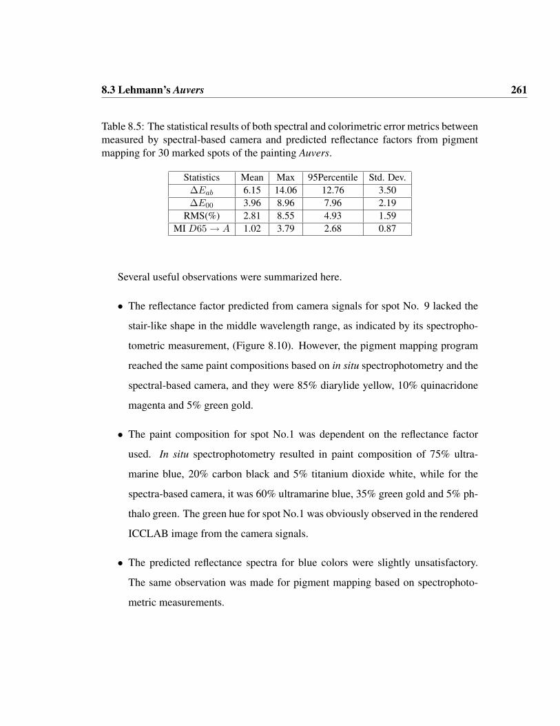
8.3 Lehmann’s Auvers 261
Table 8.5: The statistical results of both spectral and colorimetric error metrics betweenmeasured by spectral-based camera and predicted reflectance factors from pigmentmapping for 30 marked spots of the painting Auvers.
Statistics Mean Max 95Percentile Std. Dev.∆Eab 6.15 14.06 12.76 3.50∆E00 3.96 8.96 7.96 2.19
RMS(%) 2.81 8.55 4.93 1.59MI D65 → A 1.02 3.79 2.68 0.87
Several useful observations were summarized here.
• The reflectance factor predicted from camera signals for spot No. 9 lacked the
stair-like shape in the middle wavelength range, as indicated by its spectropho-
tometric measurement, (Figure 8.10). However, the pigment mapping program
reached the same paint compositions based on in situ spectrophotometry and the
spectral-based camera, and they were 85% diarylide yellow, 10% quinacridone
magenta and 5% green gold.
• The paint composition for spot No.1 was dependent on the reflectance factor
used. In situ spectrophotometry resulted in paint composition of 75% ultra-
marine blue, 20% carbon black and 5% titanium dioxide white, while for the
spectra-based camera, it was 60% ultramarine blue, 35% green gold and 5% ph-
thalo green. The green hue for spot No.1 was obviously observed in the rendered
ICCLAB image from the camera signals.
• The predicted reflectance spectra for blue colors were slightly unsatisfactory.
The same observation was made for pigment mapping based on spectrophoto-
metric measurements.

8.3 Lehmann’s Auvers 262
8.3.2.2 Pigment Mapping for Spectral Image
Finally, the small pigment maps were combined into a single map. In order to provide
better visualization of the pigment map, the concentration values were color coded.
The concentration value of one was displayed as the color of 100% paint or masstone.
The concentration value of zero was shown as a black color. The concentration value
between zero and one was coded with the tint color of the paint mixed with titanium
dioxide white.
There were twelve paints plus titanium dioxide white used in Auvers. Pigment
maps for these twelve paints were shown in Figure 8.13.

8.3 Lehmann’s Auvers 263
(a) Carbon Black (b) Ultramarine Blue (c) Cobalt Blue
(d) Yellow Ochre (e) Hansa Yellow (f) Diarylide Yellow
(g) Phthalo Green (h) Green Gold (i) Oxide Green
(j) Red Oxide (k) Pyrrole Red (l) Magenta
Figure 8.13: Pigment maps for the painting Auvers.

8.3 Lehmann’s Auvers 264
Carbon black was used in dark clouds, outlines of church, contour of dark grass,
and silhouette of the lady in front of the church. The artist might use carbon black
to delineate the drawing. The blue sky was mainly painted with ultramarine blue and
carbon black. Phthalo green and green gold might not be used in the top-left blue
sky. The greenish color in the top-left blue sky was wrong because the spectral camera
system had the problem of accurately predicting the dark colors. It was revealed that
carbon black might be used in this region through visual inspection and pigment map-
ping based on in situ spectrophotometric measurements. The road was painted with
yellow ochre. The small sands were painted with red oxide, chromium oxide green,
green gold and diarylide yellow. The orange roof was drawn with diarylide yellow, red
oxide and quinacridone magenta.
The ICCLAB image from these pigment maps was rendered for CIE illuminant
D65 and the 10-degree observer [Figure 8.14(b)]. The image displayed on a IBM LCD
monitor or printed on the paper was carefully compared with both the original painting
and the image rendered from two camera images [Figure 8.14(a)]. The blue sky of
the reproduction from these pigment maps was a little greenish and lacked the purple
blue color (the color of pure ultramarine blue). Although, the map of ultramarine blue
indicated that the blue sky was largely painted by this pigment, the purplish color of
pure ultramarine blue did not show up in the image rendered from pigment maps. The
greenish tone of the sky was caused by a small amount of chromium oxide green. Ac-
cording to the artist, yellow glaze was applied on the blue sky surrounding the church.
Since the bi-layer configuration was not taken into account in the model, it partially
explained why chromium oxide green appeared largely in the lower part of sky. Also
the prediction on the wall of the church was less greenish. Obvious banding caused by
lower spatial resolution was observed due to the simplified procedure. Pigment map-

8.3 Lehmann’s Auvers 265
ping was only done on a limited number of spots, and other pixels were mapped based
on similarity with those spots. Overall, the color appearance of the reproduction from
these pigment maps was satisfactory, and the pigment mapping was successful.
(a) Camera Signals (b) Pigment Maps
Figure 8.14: The sRGB images of the painting Auvers rendered from camera signals(a) and pigment maps (b).
8.3.3 Summary
The painting Auvers was painted by Bernard Lehmann, based on the masterpiece of
van Gogh’s The Church at Auvers. This painting was painted with 13 Golden matte
fluid acrylic paints and two acrylic color glazes. It was a very good target to test the
accuracy of both camera prediction and pigment mapping.
The painting was captured with a Sinar camera with two optimized filter. The

8.3 Lehmann’s Auvers 266
filtered tungsten light source and different exposure times for two different filters in-
creased the signal-to-noise ratio for the blue channel. The calibration target was one
traditional characterization target, ColorChecker DC, plus a custom Golden target,
which included a masstone and a tint sample for each paint in the database. After the
transformation matrix was built using the calibration targets, it was used to transform
two camera images of Auvers into spectral reflectance factor data. Both the spectral
and colorimetric accuracies of the camera system were very good.
Thirty spots in the painting were marked and measured with a contact spectropho-
tometer. Pigment mapping was first tested on these spots with spectrophotometric data,
and then with spectral reflectance factors predicted from camera signals. The resulting
spectral and colorimetric accuracies of pigment mapping based on spectrophotometric
measurements and spectral-based camera were comparable. It further proved that the
spectral accuracy of the camera system was sufficient for the purpose of pigment map-
ping. It was observed that pigment mapping for the blue-green and blue colors was
slightly worse than other colors. Due to the existence of a huge blue sky in Auvers,
the poor predictions of blue colors might affect the appearance of the entire image
drastically. The reasons might include the limited precision of concentration (5%), the
inaccuracy of the optical properties of pigments and imperfection of the two-constant
K-M theory.
The pigment mapping for the image was very satisfactory and successful. The map
of carbon black indicated that it was used to delineate the drawing. Large amount
of ultramarine blue was used in the huge blue sky. Small amount of cobalt blue was
used in the window. The main color of the sand road was made by yellow ochre, and
small sands were painted with red oxide and green gold. The orange roof was painted
with red oxide and diarylide yellow. These pigment maps can be used for different

8.4 Vincent Van Gogh’s The Starry Night 267
applications, which will be addressed in the next section with the famous painting The
Starry Night.
8.4 Vincent Van Gogh’s The Starry Night
The famous painting The Starry Night is examined extensively in this section. The
artist used both cobalt blue and ultramarine blue in the large areas of blue sky in the
painting. These two blues reflect long-wavelength light uniquely and are very sensitive
to the change in lighting. The accurate colorimetric reproduction of the painting was
very challenging. There were plenty of images of the famous painting in the internet,
but the blue sky varied a lot from blueish to purple-blueish. It was expected because
of the variation of the taking illuminants and the spectral sensitivities of the capture
devices. Furthermore, the image capture systems might not be well characterized, the
saving formats were unknown, and the display might not be characterized either.
The unframed painting was imaged with the same camera system in the conser-
vation studio of the Museum of Modern Art (MoMA), New York City. The paints
used by the artist were unknown. The first and the most important step was to select
several paints to form van Gogh’s palette. After that, the pigment mapping was done
with these selected paints. Also, the color appearance of the painting was simulated
when the optical properties of one or more paints were modified. For example, the lead
white paint used in the painting has darkened observably. The optical property of the
“aged” lead white can be replaced with that of the “fresh” lead white, and the change
of color appearance of The Starry Night was simulated (this operation is also referred
as digitally rejuvenation (Berns et al., 2006)).

8.4 Vincent Van Gogh’s The Starry Night 268
8.4.1 Spectral-Based Camera
The same camera system was used. The spectral power distribution of the light source
is shown in Figure 8.15. The light source, with CCT of 4462K, was more balanced
than tungsten light in the visible range.
Figure 8.15: Spectral power distribution of the light source at MoMA.
One major camera defect was discovered. In the horizontal center of the image
plane, there was a high frequency black-white noise pattern, shown in Figure 8.16,
which only affected camera signals in that region. The flat fielding could not eliminate
this noise pattern, and might even deteriorate the problem if two camera images of the
white board used for flat fielding were mis-registered. So the flat fielding was skipped.
Due to complex content of the painting The Starry Night, the noise pattern in their
camera images was less observable.

8.4 Vincent Van Gogh’s The Starry Night 269
Figure 8.16: Nose pattern in the image of white board taken through yellow filter.
The ColorChecker DC and ESSER targets were used as the calibration and inde-
pendent verification targets, respectively. The colorimetric and spectral accuracies are
summarized in Table 8.6. The accuracies for the calibration target was sufficient, while
the accuracies for the verification target was just acceptable. The learning-based recon-
struction depends critically on the calibration target. If the verification target is very
different from the calibration target, the performance for the verification target will
be unsatisfactory. However, it is known that ESSER target is very similar to CCDC
target. The poor accuracies of ESSER target were caused by the camera noise. The
CCDC target located in the middle noise region, and the ESSER was in the bottom of
the image plan. The difference between the CCDC and ESSER targets were caused
by the existence and absence of the camera noise. A large number of pixels were av-
eraged for each patch for these two targets. The accuracies were evaluated based on
the average patch data. Due to the existence of the camera noise, other targets, e.g.,
two Golden targets (Big Squares and Small Squares) were not used in both the cali-
bration and verification. For the previous case study, the painting Auvers was imaged
later in the Munsell Color Science Lab. Because of the existence of the camera noise,

8.4 Vincent Van Gogh’s The Starry Night 270
all the targets plus the painting only occupied the lower half of the image plane. The
mean color difference CIEDE2000 for CCDC and ESSER when CCDC used as the
calibration target were 0.79 and 1.12 ∆E00 (Table 8.2), while the mean spectral RMS
errors were 1.37% and 1.66% (Table 8.1). The colorimetric and spectral accuracies
were significantly improved when only half the image plane was used.
Table 8.6: The statistical results of both spectral and colorimetric error metrics betweenmeasured and predicted reflectance factors from camera signals for both CCDC andESSER targets
Calibration Target - CCDCStatistics Mean Max 95Percentile Std. Dev.∆Eab 2.08 19.01 6.53 2.44∆E00 1.23 9.86 2.89 1.14
RMS(%) 1.61 8.47 3.20 0.99MI D65 → A 0.74 8.55 2.97 1.01
Verification Target - ESSERStatistics Mean Max 95Percentile Std. Dev.∆Eab 4.29 25.49 16.81 4.92∆E00 2.52 17.09 5.95 3.02
RMS(%) 2.75 11.42 4.93 1.42MI D65 → A 0.92 4.94 2.71 0.88
Next, the camera accuracy was evaluated with spot measurements of the painting.
The sRGB representation of the painting along with 20 spots is shown in Figure 8.17.
Because it was difficult to exactly locate each measured spot in the painting, the pre-
dicted reflectance factors of all the pixels in the vicinity of estimated measurement
spot were compared with the corresponding spot measurement, and the one that was
the best match to the measurement was selected. It was expected that the performance
was obviously better when selecting the best match in the vicinity of each spot, instead
of averaging the reflectance spectra over each spot.

8.4 Vincent Van Gogh’s The Starry Night 271
Figure 8.17: The sRGB representation of reconstructed spectral image of the paintingThe Starry Night painted by Vincent van Gogh along with 20 marked measurementspots.
The measured and predicted reflectance factors from the camera signals are plot-
ted in Figure 8.18. For most spots, the predicted reflectance factors from the cam-
era signals followed the corresponding measurements well, especially for the yellow
and orange colors patches. The predicted reflectance factors had wave-like shape for
patches No. 15 (canvas) and 16 (white) because of the transformation matrix from the
camera signals to reflectance factors, discussed in Chapter 5. For the two blue patches,
the predicted reflectance factors could not match the measured ones well, especially in
the longer wavelengths. It was because the calibration target CCDC lack of spectral
variability in that wavelength region. However, the customized paint target was not

8.4 Vincent Van Gogh’s The Starry Night 272
used to calibrate the camera system because of the existence of the camera noise in the
middle of the image plane. The statistical results are summarized in Table 8.7. Both
the spectral and colorimetric accuracies were acceptable, and pigment mapping was
performed next.
Figure 8.18: Measured (red line) and predicted reflectance factors (blue line) from thecamera signals for 20 measured spots in the paining The Starry Night.
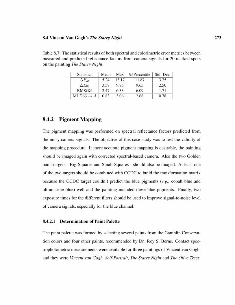
8.4 Vincent Van Gogh’s The Starry Night 273
Table 8.7: The statistical results of both spectral and colorimetric error metrics betweenmeasured and predicted reflectance factors from camera signals for 20 marked spotson the painting The Starry Night.
Statistics Mean Max 95Percentile Std. Dev.∆Eab 5.24 13.17 11.87 3.25∆E00 3.58 9.75 9.65 2.50
RMS(%) 2.47 6.33 6.09 1.71MI D65 → A 0.83 3.06 2.68 0.78
8.4.2 Pigment Mapping
The pigment mapping was performed on spectral reflectance factors predicted from
the noisy camera signals. The objective of this case study was to test the validity of
the mapping procedure. If more accurate pigment mapping is desirable, the painting
should be imaged again with corrected spectral-based camera. Also the two Golden
paint targets - Big-Squares and Small-Squares - should also be imaged. At least one
of the two targets should be combined with CCDC to build the transformation matrix
because the CCDC target couldn’t predict the blue pigments (e.g., cobalt blue and
ultramarine blue) well and the painting included these blue pigments. Finally, two
exposure times for the different filters should be used to improve signal-to-noise level
of camera signals, especially for the blue channel.
8.4.2.1 Determination of Paint Palette
The paint palette was formed by selecting several paints from the Gamblin Conserva-
tion colors and four other paints, recommended by Dr. Roy S. Berns. Contact spec-
trophotometric measurements were available for three paintings of Vincent van Gogh,
and they were Vincent van Gogh, Self-Portrait, The Starry Night and The Olive Trees.

8.4 Vincent Van Gogh’s The Starry Night 274
These three paintings were all painted in 1889. The artist might use the same pig-
ments in all three paintings. Finally, ten pigments were selected to form Vincent van
Gogh’s palette. These ten pigments included cobalt blue, ultramarine blue, Prussian
blue, zinc yellow, cadmium lemon yellow, indian yellow, earth yellow, emerald green,
burnt sienna and “aged” lead white. “Aged” lead white was obtained from the contact
measurements of Seurat’s A Sunday Afternoon on the Island of La Grande Jatte (1884-
1886) (Berns et al., 2006). Cadmium lemon yellow came from a pigment database
at the National Gallery of Art, Washington DC. Zinc yellow and emerald green were
measured from the paint samples.
White Paint There were three possible white paints: zinc white, titanium dioxide
white and lead white. The use of lead white paint was common in 1889, but not so
often nowadays because lead is poisonous and lead paint will become discolored over
a long period time. Measured reflectance factors for these white paints are plotted in
Figure 8.19. The measurement of the “aged” lead white paint was obtained from the
white sailcloth in Seurat’s painting A Sunday Afternoon on the Island of La Grande
Jatte (1884-1886) (Berns et al., 2006). The reflectance factor of the “fresh” lead white
was also measured. The measured reflectance factors of the white colors in two van
Gogh’s paintings – The Starry Night (abbreviated as SN) and The Olive Tree (OT) –
are also plotted. It was obvious that aged lead white, the white in Seurat’s painting,
was the most appropriate representation of the white pigment for The Starry Night.

8.4 Vincent Van Gogh’s The Starry Night 275
Figure 8.19: Measured spectral reflectance factors for several possible white paints andwhite colors in the paintings (SN: The Starry Night OT: The Olive Tress).
Emerald Green This paint has the most beautiful and the most intense green color,
but it is chemically unstable and very poisonous arsenic. The reflectance factor of
this pigment is plotted in Figure 8.20, along with measured green colors from three
van Gogh’s paintings. The painting Vincent van Gogh, Self Portrait was abbreviated
as SP. Although these spectra all had one single peak around 530nm, the measured
reflectance spectra from the paintings were much broader than that of “fresh” emer-
ald green. The green colors in these paintings might have changed chemically after
more than one hundred years, and they might also be mixed with either white or other
paints. However, the measured reflectance factor of the fresh emerald green was used
to calculate the optical property of this green pigment and included in the palette.

8.4 Vincent Van Gogh’s The Starry Night 276
Figure 8.20: Measured spectral reflectance factors for 100% emerald green (green solidline) and some green colors in the paintings. Black line: Self Portrait (SP) Red line:The Starry Night (SN) and Blue line: The Olive Tree (OT)
Blue Paints Three blue pigments – cobalt blue, ultramarine blue and Prussian blue
– are plotted in Figure 8.21, along with the blue colors measured from two van Gogh
paintings, The Starry Night and The Olive Trees. The three blue pigments had quite
unique long-tails. Except for one spot color No. 9 in the painting The Olive Trees,
the blue colors measured in both paintings had the long-tail of the ultramarine blue.
It appeared that cobalt blue was used in spot No. 9 in The Olive Trees. The peak
widths of these colors in the short-wavelength had small variations. The cobalt blue
and ultramarine blue used by the artist at that time might be slightly different from
the modern counterparts. Prussian blue had a broader peak than ultramarine blue.
Although Prussian blue might not be used by the artist, it was selected in the palette.
It was found later that Prussian blue was used in predicting dark brown, dark blue and
some green colors from results of pigment mapping. All three blue pigments were
included in the palette.

8.4 Vincent Van Gogh’s The Starry Night 277
(a) Three Possible Blue Paints (b) Blue Colors in Paintings
Figure 8.21: Measured spectral reflectance factors for 3 blue paints (a) and some bluecolors (b) in the paintings. Blue line: The Starry Night (SN) and Red line: The OliveTrees (OT)
Yellow Paints The yellow pigments were really hard to decide. Eight possible yellow
pigments included zinc yellow, cadmium lemon yellow, earth yellow, yellow ochre,
hansa yellow medium, cadmium yellow light, cadmium yellow medium and indian
yellow. Spectral reflectance factors of these yellow pigments and some yellow colors
measured in the paintings are plotted in Figure 8.22. The selection of yellow pigments
was mainly based on the edge of the spectrum or the inflection point in the middle-
wavelength range. The yellow colors of the paintings had roughly four locations of
edges, and they were 500nm, 510nm, 530nm and 540nm, so four yellow pigments
were selected. Several yellow pigments had very similar spectrum, for example, zinc
yellow and cadmium yellow light, indian yellow and cadmium yellow medium, and
earth yellow and yellow ochre. Finally, cadmium lemon yellow, zinc yellow, indian
yellow and earth yellow were chosen.

8.4 Vincent Van Gogh’s The Starry Night 278
(a) Possible Yellow Paints
(b) Yellow Colors in Paintings
Figure 8.22: Measured spectral reflectance factors for several yellow paints (a) andsome yellow colors (b) in the paintings. Red line: The Starry Night (SN) and Blueline: The Olive Trees (OT)
Other Paint The last pigment in the palette was burnt sienna. The spectral re-
flectance factor of this paint is plotted in Figure 8.23 (a). It was found from pigment
mapping that this pigment was largely used to predict red and dark colors, as shown in
Figure 8.23 (b). Nos. 4-6 were measured around the cypress and No. 8 was measured
at the dark mountain (in the middle right of the painting). Vincent van Gogh did not

8.4 Vincent Van Gogh’s The Starry Night 279
use black pigment in his paintings, so no black paint was chosen.
(a) Burnt Sienna (b) Dark Colors in the Painting
Figure 8.23: Measured spectral reflectance factors for 100% burnt sienna and somedark colors in the painting The Starry Night.
8.4.2.2 Pigment Mapping for Measurement Spots
Since one measurement was available for each paint in the palette, the pigment map-
ping was only done using single-constant K-M theory, where the ratio between absorp-
tion and scattering for each paint was calculated from one reflectance measurement.
The mapping method used was still the exhaustive search. The combination of three
paints plus white paint was found to be the best match of the reflectance factor for each
spot. The measured and predicted reflectance factors from pigment mapping for 20
measurement spots are plotted in Figure 8.24. The predicted reflectance factors fol-
lowed the measured ones closely. It proved that the selected paints in the palette could
cover the spectral variability of the painting, and the simplified single-constant model
was acceptable.

8.4 Vincent Van Gogh’s The Starry Night 280
Figure 8.24: Measured (red line) and predicted reflectance factors (blue line) frompigment mapping for 20 measured spots in the paining The Starry Night.
The pigment mapping was also done with predicted reflectance factors from camera
signals. The statistical results are also provided in Table 8.8. The prediction accuracies
of pigment mapping based on spectrophotometric measurements and spectral-based
camera were not statistically different. It further confirmed that the spectral accuracy
of the camera system was sufficient for pigment mapping.
8.4 Vincent Van Gogh’s The Starry Night 281
Table 8.8: The statistical results of both spectral and colorimetric error metrics be-tween measured and predicted reflectance factors from pigment mapping based on thespectrophotometric measurement and camera prediction.
Spectrophotometric MeasurementsStatistics Mean Max 95 Percentile Std. Dev.∆Eab 4.88 13.62 12.05 3.12∆E00 3.22 7.33 7.14 1.96
RMS(%) 1.93 4.69 4.62 1.45MI D65 → A 0.52 1.58 1.47 0.42
Spectral-Based CameraStatistics Mean Max 95 Percentile Std. Dev.∆Eab 5.56 18.31 15.71 4.48∆E00 3.83 11.81 10.82 3.18
RMS(%) 2.20 4.44 4.34 1.23MI D65 → A 0.97 2.43 2.33 0.66
8.4.2.3 Pigment Mapping for Spectral Image
The pigment maps for these paints are plotted in Figure 8.25. The large areas of blue
sky was undoubtedly painted with both ultramarine blue and cobalt blue. This finding
that both blue pigments were used in the painting was unexpected. Contact spec-
trophotometric measurements in The Starry Night indicated that only ultramarine blue
was used (Figure 8.21). Only two blue colors in The Starry Night were measured,
and these two colors were made up of ultramarine blue, which was revealed from its
pigment map. It implied that more contact measurements in different regions were
necessary to detect the hidden pigments.
The stars and the moon were most likely painted with indian yellow and zinc yel-
low. The light green cloud surrounding the moon was probably painted with emerald
green. The cypress tree might be painted with burnt sienna and Prussian blue. Cad-
mium lemon yellow might be used to paint the yellow clouds surrounding the moon

8.4 Vincent Van Gogh’s The Starry Night 282
and the stars.
(a) Ultramarine Blue (b) Cobalt Blue (c) Prussian Blue
(d) Indian Yellow (e) Zinc Yellow (f) Lemon Yellow
(g) Emerald Green (h) Burnt Sienna (i) Earth Yellow
Figure 8.25: Pigment maps for the paining The Starry Night.
The maps of Prussian blue and earth yellow indicated that they were used almost
in the entire painting. It was very unlikely that the artist used these two paints in
the whole painting. Even though these two concentration maps had a low credibility,
existence of these two paints certainly helped improving the prediction accuracy of
pigment mapping. The spectral reflectance curves for these two paints were relatively

8.4 Vincent Van Gogh’s The Starry Night 283
flat, and incorporating these two pigments in the pigment-mixing model could improve
the prediction. Since the painting have been exhibited for more than one hundred
years, it was possible that some paints had been changed chemically. In addition,
the modern paints, e.g., ultramarine blue and cobalt blue, might be different from the
old paints in the painting, which was revealed from Figure 8.21. A small amount of
Prussian blue in the large area of blue sky might help compensating this difference.
But most importantly, it implied that one or more paints used by the artist might not be
discovered. Further modern analysis techniques, e.g., X-ray fluorescence spectroscopy,
are necessary.
The image rendered from pigment maps was compared with the image calculated
from camera signals for the same illuminant and observer, shown in Figure 8.26. As
a whole, the reproduction from camera signals was more colorful and vivid, while
reproduction from the pigment maps was slightly pale and washed-out. The blue sky in
the top-left corner of the reproduction from these pigment maps also lacked the purple
blue color (the color of pure ultramarine blue). Also, the pigment map indicated that
this area of blue sky was painted with this pigment. Because of the large area of purple
blue sky, it was very important to accurately reproduce this color. In addition, it was
found that this color exhibited perceptible color change with the change of illuminants
and viewing angle. The exact colorimetric reproduction of this blue sky was very
difficult. The optical properties of ultramarine blue should be carefully examined, and
more paint samples should be prepared and used to test the prediction accuracy of the
pigment-mixing model. Considering the imprecision camera system (high frequency
noise in the middle of image plane and the inaccurate pigment-mixing model (single-
constant K-M theory), the pigment mapping was satisfactory.

8.4 Vincent Van Gogh’s The Starry Night 284
(a) Camera Signals
(b) Pigment Maps
Figure 8.26: The sRGB images of the painting The Starry Night rendered from camerasignals (a) and pigment maps (b).

8.4 Vincent Van Gogh’s The Starry Night 285
8.4.2.4 An Application
These pigment maps could be used to simulate the change of color appearance of The
Starry Night and to provide the guidance for retouching. One possible application was
to digitally rejuvenate the paining if the lead paint had not darkened. The reflectance
factors of both fresh and aged lead white were plotted in Figure 8.19. The ratios be-
tween absorption and scattering for both fresh and aged lead white paints were calcu-
lated. The image could be simulated from the pigment maps and these ratios for all the
paints in the palette except that the ratio for the aged lead white was replaced with that
for the fresh lead white. The simulated and the original images rendered with the aged
lead white are shown in Figure 8.27. The color appearance between these two images
had drastic difference around the star. The lightness of these colors surrounding the
star increased significantly when the aged lead white was replaced with fresh one.
(a) Aged Lead White (b) Fresh Lead White
Figure 8.27: Two sRGB images rendered from pigment maps with both aged and freshlead white.

8.4 Vincent Van Gogh’s The Starry Night 286
8.4.3 Summary
The paints used by the artist in The Starry Night were unknown. The van Gogh’s
palette approximated using six oil pigments selected from twenty-eight Gamblin Con-
servation Colors and four additional oil colors based on historical knowledge of van
Gogh’s working method. These four colors were zinc yellow, cadmium lemon yellow,
emerald green and aged lead white. Both emerald green and lead white are known to
be unstable and poisonous, and no longer commonly used in modern paintings. Except
for these four colors, cobalt blue, ultramarine blue, indian yellow, burnt sienna, earth
yellow and Prussian blue were selected in the palette.
Several useful conclusions could be drawn from the visual inspection of pigment
maps. The large area of blue sky was certainly painted with both ultramarine blue and
cobalt blue. The stars and the moon were most likely painted with indian yellow and
zinc yellow. The light green cloud surrounding the moon was probably painted with
emerald green. The cypress tree might be painted with burnt sienna and Prussian blue.
Cadmium lemon yellow might be used to paint the yellow clouds surrounding the moon
and the stars. Two paints, Prussian blue and earth yellow, might not be the right paints
to map the painting since the maps indicated that these two paints were used almost
in the entire painting. However, their existence could improve the prediction accuracy
of pigment mapping and also compensate the difference between modern paints and
paints in the painting. Most importantly, it implied that one or more paints used by the
artist might not been discovered. The discovery of those unknown pigment required
further modern analysis techniques, e.g., X-ray fluorescence spectroscopy.
These pigment maps can be used to simulate the change of color appearance of the
painting and also provide guidance for retouching. The simulation of The Starry Night
with fresh lead white were very exciting.

8.5 Conclusions 287
8.5 Conclusions
Two paintings were studied. Auvers was painted by the local artist, Bernard Lehmann,
which was a copy of Vincent van Gogh’s The Church at Avuers. The other painting
was the famous masterpiece The Starry Night, pained by Vincent van Gogh in 1889.
The second painting is part of the permanent collection of the Museum of Modern Art
in New York City. The major similarity between these two paintings was the blue sky,
and both cobalt blue and ultramarine blue were used in these two paintings.
Auvers was painted with Golden matte fluid acrylic paints and color glazes. These
paints were characterized on an absolute basis using the two-region method (Chapter
6). The pigment-mixing model was the two-constant K-M theory under the opaque and
single-layer assumptions. The paints used in The Starry Night were unknown. A paint
palette included six selected paints from the Gamblin conservation colors and four
additional colors based on historical knowledge of van Gogh’s working method. Since
only one reflectance measurement was available for each paint, the pigment mixing
model was the single-constant K-M theory for the opaque case.
The pigment mapping for both paintings was very satisfactory and successful. It
proved that the spectral accuracy of the spectral-based camera was sufficient enough
for analyzing the paint composition pixel-wise. It also demonstrated pigment mapping
as a viable practical method. With these pigment maps, the change of color appear-
ance was simulated. The simulations of The Starry Night with fresh lead white was
very exciting. Finally, the pigment maps can also aid conservators for retouching and
provide valuable historical knowledge of the painting.
Chapter 9
Conclusions and Perspectives
9.1 Conclusions
The conclusions for this dissertation research are summarized as follows.
1. A new spectral reconstruction method, called the Matrix R method, was brought
forth based on the Wyszecki hypothesis and the matrix R theory developed by
Cohen and Kappauf. The spectral reflectance factor was retrieved by combining
the fundamental stimulus predicted from colorimetric transformation with the
metameric black estimated from spectral transformation. So the new method
combined the benefits of both colorimetric and spectral transformations, and
achieved high spectral and colorimetric accuracies for a certain combination of
observer and illuminant at the same time.
2. Pigment database development is a laborious and time-consuming process. Com-
mon practice requires the preparation of a tint ladder consisting of five or more
samples per pigment in order to characterize the optical properties of each pig-

9.1 Conclusions 289
ment. It was found that only two samples – one pure pigment (or masstone) and
one mixture sample with white paint – were sufficient to characterize each pig-
ment. For the opaque case, these two samples should be applied to full-opacity.
For the translucent case, each pigment should be characterized on an absolute
basis and as a function of thickness, and these two samples should be prepared
on an opacity chart including both a white and a black background with the
same film thickness. The sample preparation for the translucent case was even
harder with the strict requirement on the film thickness. There were four pig-
ment databases available, where the value in parenthesis indicates the number of
pigments included in the database.
Gamblin Conservation Colors (28) The ratio between absorption and scatter-
ing coefficients for each paint was calculated based on single-constant K-M
theory.
Gamblin artist oil paints (11) Both absorption and scattering coefficients for
each paint were calculated based on masstone-tint method for the opaque
case. The scattering coefficient for the white paint was assumed to be one
at all wavelengths.
Golden Matte Fluid Acrylic Paints (28) The same as the Gamblin artist oil
paints.
Golden Matte Fluid Acrylic Paints (16) and Acrylic Color Glazes (4) Both ab-
sorption and scattering coefficients for each paint were calculated on an
absolute basis using the two-region method and the general from of K-M
theory.
3. Compared with conventional color imaging, spectral imaging takes advantage

9.1 Conclusions 290
of much more embedded information in spectral reflectance. The spectral ac-
curacy of the matrix R method was further improved by incorporating pigment
mapping. A virtual camera model was simulated and used along with a custom
target including four Golden artist paints to verify the recovery of the smoothness
of spectral reflectance predicted by the original matrix R method. Incorporating
pigment mapping reduced the mean RMS error for the custom target from 3.8%
to 1.1% and the maximum RMS error by almost two fold. It also decreased
the degree of metamerism appreciably. By incorporating pigment mapping, the
improved matrix R method achieved even higher spectral accuracy.
4. Four methods for determining the absorption and scattering coefficients of translu-
cent paints were reviewed including detailed mathematical derivations. They
were the black-white method, the infinite method, the masstone-tint method and
the two-region method. The two-region method was used to characterize a set
of acrylic-emulsion artist paints and glazes spanning a range of opacities from
opaque to nearly transparent. The optical characterization was tested using mix-
tures of single or two chromatic paints with and without the white paint. Concen-
tration was estimated for each mixture and for both backgrounds using the gen-
eral form of the K-M equation and constrained nonlinear optimization where the
objective function was to minimize spectral RMS error between measured and
predicted reflectance factors. Performance was acceptable with average color
difference CIEDE2000 of about 2 ∆E00 and less than 2% RMS error. As a
comparison, concentration was estimated using the opaque simplification with
the same optical database and optimization algorithm. Performance was statis-
tically significantly worse with an average color difference of about 3.5 ∆E00
and above 3% RMS spectral error. For samples with appreciable error, the cause

9.1 Conclusions 291
was traced principally to variability in film thickness leading to errors in the op-
tical constants. The general form of Kubelka-Munk turbid media theory can be
applied effectively to translucent and opaque paint films providing that sample
preparation and spectral measurements have high precision, particularly prepar-
ing samples with uniform and reproducible film thickness.
5. The pigment mapping method used was an exhaustive search algorithm written
in the C language. The objective function minimized the spectral RMS error
between measured and predicted reflectance factors. One obvious shortcoming
of this method was that it tended to choose more pigments than necessary to
achieve the best match to the specified reflectance spectrum. To overcome the
problem of over-fitting, the maximum number of paints in each mixture was
limited to three. Except for the over-fitting problem, there were two major rea-
sons to explain why the program could not find the right paint compositions for
some mixtures. First, two reflectance spectra might be very close to each other
but had quite different paint compositions. Next, the accuracy of the forward
pigment mapping was limited because of the inaccuracy of the pigments’ optical
properties as functions of thickness, imprecision of reflectance measurement and
imperfectness of K-M theory.
6. The knowledge of opacity and layer configuration was not so beneficial to im-
prove the accuracies of both pigment identification and mapping. Incorporating
the inaccuracy of the camera system, the advantage of knowing the opacity and
layer configuration was even less pronounced. For paintings, it was impossible to
know the paint composition for each pixel, so the correctness of pigment identifi-
cation and accuracy of concentration prediction could not be done on pixel-wise
basis. The possible error metrics for paintings were the colorimetric and spec-
9.1 Conclusions 292
tral accuracies of reflectance factors predicted from camera signals and pigment
maps. So for paintings, the simple opaque model under single-layer assumption
should be used to do pigment mapping with the objective of minimizing spectral
RMS error.
7. A practical pigment mapping procedure was proposed. A large image was first
partitioned into several small images, and each small image was segmented into
different clusters using either unsupervised or supervised image classification.
There were two different strategies to do pigment mapping pixel-wise. One
strategy was to map constituent pigments and their concentrations for each pixel
with a limited number of paints. Another strategy was to do pigment mapping
on a limited number of selected pixels, and then to map the other pixels based on
similarity calculation in camera space between each pixel of interest and these
selected pixels. Finally, the pigment map for each pigment of the entire image
was combined from several small maps.
8. A small oil painting Flowers in a Blue Vase was painted with eleven Gamblin
artist oil paints. The painting was first segmented into five clusters using un-
supervised K-Means classification in two-chromatic space (a∗, b∗), and for each
cluster, at most four pigments were selected to map each pixel in the cluster. The
computation efficiency was improved by focusing on a limited number of pixels
rather than unmixing with the entire pigment database.
9. The painting Auvers was painted with Golden matte fluid acrylic paints and
acrylic color glazes by the artist Bernard Lehmann, based on the masterpiece
of Vincent van Gogh’s The Church at Auvers. The pigment maps provided some
useful information. The map of carbon black indicated that it was used to delin-

9.1 Conclusions 293
eate the drawing. Large amount of ultramarine blue was used in the huge blue
sky. A small amount of cobalt blue was used in the window. The main color of
the sand road was made by yellow ochre, and small sands were painted with red
oxide and green gold. The orange roof was painted with red oxide and diarylide
yellow. The image rendered from pigment maps for CIE illuminant D65 and
the 10-degree standard observer was printed and compared with the painting.
Except for slightly hue shift of the blue sky, the colorimetric accuracy of repro-
duced image was satisfactory through visual inspection. So pigment mapping
for Auvers was successful.
10. The original The Starry Night was painted by Vincent van Gogh with unknown
oil pigments. Vincent van Gogh’s palette was first approximated using six se-
lected oil pigments from Gamblin conservation colors and four additional paints
based on historical knowledge of van Gogh’s working method. Several useful
conclusions were drawn from the visual inspection of pigment maps. The mas-
sive blue sky was certainly painted with both ultramarine blue and cobalt blue,
two pigments used extensively by Vincent van Gogh at this stage of his career.
The stars and the moon was painted with indian yellow and zinc yellow with
very high probability. The light green cloud surrounding the moon was probably
painted with emerald green. The cypress tree might have been painted with burnt
sienna and Prussian blue. Three paints, cadmium lemon yellow, Prussian blue
and earth yellow, might not be the correct paints to map the painting because
their maps indicated that a small amount of these paints existed everywhere in
the painting. The discovery of these unknown pigments requires further modern
analysis techniques, e.g., X-ray fluorescence spectroscopy. These pigment maps
can be used to simulate the change of color appearance of the painting. The

9.2 Perspectives 294
simulation of The Starry Night with fresh lead white was very exciting.
11. Pigment mapping of a painting was viable based on spectral imaging. With
these pigment maps, the change of color appearance can be simulated when the
optical properties of some pigments are replaced with those of other pigments.
Also, these pigment maps will be beneficial for enriching the historical knowl-
edge of the painting and will aid conservators in determining the best course for
retouching damaged areas on the painting.
9.2 Perspectives
Time did not allow full exploration of all of the ideas that were suggested in the dis-
cussions around this dissertation. In the following, possible future work is discussed.
• The newly proposed reconstruction method, matrix R method, can be further
improved by replacing the tristimulus integration weights used as additive pri-
maries with primaries that better represent complex-subtractive pigments. These
three primaries can be three eigenvectors (or independent components) based on
principal component analysis (PCA) (or independent component analysis) of a
spectral reflectance database.
• The spectral transformation from camera signal to spectral reflectance factor is
simply based on linear-least-square method without any constraint. The pre-
dicted reflectance factor might be negative or greater than one. One could con-
strain the transformation such that the predicted reflectance factor is always be-
tween zero and one.

9.2 Perspectives 295
• More computationally efficient methods of pigment mapping need to be devel-
oped. Smart pigment selection routines should be explored to reduce the number
of possible paints in the model. Optimization routines should be developed to
find the optimal pigment concentrations and the film thickness. These methods
should still be implemented in efficient C language.
• Pigment mapping finds the constituent pigments and their concentrations, which
is very similar to ink separation for a printer. Several spectral-based printing
technologies have been developed based on multi-dimensional look-up-tables
(LUTs) in recent years. Because of similarity between pigment mapping and
ink separation, it might be possible to perform pigment mapping based on multi-
dimensional LUT. Although it takes time to build the LUT, it will be much faster
to process the entire image. The size of the LUT depends on both the number of
paints and the grid size. For example, if the number of paints is six and the grid
size is 17 (concentration precision is 6.25%), the size of LUT is about 46MB.
If the number of paints increases, the size of the LUTs increases exponentially.
To avoid large LUT, it is better to build several small LUTs. The image would
first be segmented into different clusters, and each cluster will be processed with
a small LUT including a limited number of paints.
• Semi-supervised classification algorithms, which combine labeled and unlabeled
data during training to improve performance, should be developed. In supervised
classification, there are a known fixed set of clusters and cluster-labeled training
data are used to induce a classification function. On the other hand, the unsuper-
vised classification, e.g., K-means, iteratively updates the center of each cluster
until the change is negligible. The only required input for the K-Means classi-
fication is the number of clusters. The purpose of image segmentation in this

9.2 Perspectives 296
dissertation was to partition a image into different clusters, and for each cluster,
pigment mapping was done with a limited number of pigments. It is easy to label
training data for some clusters but not all of them based on expert experience. So
semi-supervised clustering is a more proper method, where some labeled data is
used along with the unlabeled data to obtain a better clustering.

Appendix A
Nature of Spectral Reflectance
A.1 Introduction
Spectral reflectance is a physical characteristic of an object surface, while color is a
psychophysical perception that depends on many factors such as the illumination, the
observer and surround conditions. Besides, color can be easily deducted from spec-
tral reflectance. So it is more useful to know spectral reflectance of a surface than to
know its color. Furthermore it implies that spectral color reproduction, which depicts
each scene pixel spectrally, is more powerful than traditional colorimetric reproduc-
tion, which represents each pixel colorimetrically.
First, spectral reflectance databases used in the analysis are introduced. Then dis-
crete Fourier transforms are performed on these databases to prove that they are band
limited because of the smoothness of spectral reflectance curves. After that, principal
component analysis is used to analyze the databases, and it is found that six eigenvec-
tors can explain almost all the variance. Finally, these databases are plotted in CIELAB
to visually study the similarity and dissimilarity between these data sets.

A.2 Spectral Reflectance Databases 298
A.2 Spectral Reflectance Databases
There are six spectral reflectance databases in the analysis, listed in Table A.1. The
spectral reflectance factors were measured using Macbeth SpectroEye spectropho-
tometer with 45/0 geometry, and the wavelength range was from 380 nm to 730 nm
with 10 nm increment.
Table A.1: Lists of the names, abbreviations and number of patches in each of sixtargets
No. Name Abbreviation No. of Patches1 GretagMacbeth ColorChecker DC CCDC 2402 GretagMacbeth ColorChecker CC 243 ESSER TE221 scanner target ESSER 2644 A custom target of Gamblin conservation colors Gamblin 605 An acrylic-medium blue target Blue 566 Two small oil paintings Fish & Flower 22
A.3 Fourier Analysis
Generally speaking, spectral reflectance curves are fairly smooth, so they are band lim-
ited, which can be proved by performing a Fourier analysis over spectral reflectance
databases. For each spectral reflectance factor, its power spectrum can be calculated us-
ing Eq. (A.1), where S is the power spectrum of the reflectance spectrum R, supscript
∗ represents complex conjugate operation, FFT is the abbreviation of Fast Fourier
Transform and FFT (R, 128) means that reflectance spectrum is first padded with
trailing zeros to length of 128 and then used in a discrete fast Fourier transform.

A.3 Fourier Analysis 299
S =1
128[FFT (R, 128)] [FFT (R, 128)]∗ (A.1)
0 10 20 300
2
4
6
Frequency
Pow
er S
pect
rum
ColorChecker DC
0 10 20 300
2
4
6
Frequency
Pow
er S
pect
rum
ColorChecker
0 10 20 300
1
2
3
Frequency
Pow
er S
pect
rum
ESSER
0 10 20 300
1
2
3
4
Frequency
Pow
er S
pect
rum
Blue
0 10 20 300
1
2
3
Frequency
Pow
er S
pect
rum
Gamblin
0 10 20 300
2
4
6
Frequency
Pow
er S
pect
rum
Fish&Flower
Figure A.1: Power spectra of spectral reflectance factors for all the databases
Figure A.1 shows the power spectra for all the databases. These power spectra
are averaged to obtain mean power spectrum for each database, shown in Figure A.2.
The threshold frequency is defined as the frequency when the value of mean power
spectra is smaller than 0.005. Above the threshold there will be nearly no presence
of frequency component. The threshold frequencies for these six targets are listed in
Table A.2. It can be easily concluded that these targets are indeed band limited. The
smoothness of spectral reflectance curves determines that they are band limited and
there are some correlations between sample points of the curves.

A.3 Fourier Analysis 300
0 5 10 15 20 25 300
0.2
0.4
0.6
0.8
1
1.2
1.4
1.6
Frequency
Mea
n P
ower
Spe
ctru
m
ColorChecker DC
ColorChecker
ESSER
Blue
Gamblin
Fish&Flower
Figure A.2: Mean power spectra for six databases
Table A.2: Results of Fourier Transform
Data Set CCDC CC ESSER Gamblin Blue Fish & FlowerThreshold Frequency 18 15 12 16 15 18

A.4 Principal Component Analysis (PCA) 301
A.4 Principal Component Analysis (PCA)
Principal component analysis, abbreviated as PCA, is a well-known statistical tool that
transforms a number of correlated variables to a small number of uncorrelated variables
called principal components. The PCA is used to statistically analyze these databases,
and the first six eigenvectors for each database are plotted in Figure A.3.
400 600
−0.4
−0.2
0
0.2
0.4
0.6
Pse
udo−
refle
ctan
ce
400 600
−0.4
−0.2
0
0.2
0.4
0.6
PCA Analysis for ColorChecker DC
400 600
−0.4
−0.2
0
0.2
0.4
0.6
400 600
−0.4
−0.2
0
0.2
0.4
0.6
Wavelength λ, nm
Pse
udo−
refle
ctan
ce
400 600
−0.4
−0.2
0
0.2
0.4
0.6
Wavelength λ, nm400 600
−0.4
−0.2
0
0.2
0.4
0.6
Wavelength λ, nm
(a) CCDC
400 600
−0.4
−0.2
0
0.2
0.4
0.6
Pse
udo−
refle
ctan
ce
400 600
−0.4
−0.2
0
0.2
0.4
0.6
PCA Analysis for ColorChecker
400 600
−0.4
−0.2
0
0.2
0.4
0.6
400 600
−0.4
−0.2
0
0.2
0.4
0.6
Wavelength λ, nm
Pse
udo−
refle
ctan
ce
400 600
−0.4
−0.2
0
0.2
0.4
0.6
Wavelength λ, nm400 600
−0.4
−0.2
0
0.2
0.4
0.6
Wavelength λ, nm
(b) CC
400 600
−0.4
−0.2
0
0.2
0.4
0.6
Pse
udo−
refle
ctan
ce
400 600
−0.4
−0.2
0
0.2
0.4
0.6
PCA Analysis for ESSER
400 600
−0.4
−0.2
0
0.2
0.4
0.6
400 600
−0.4
−0.2
0
0.2
0.4
0.6
Wavelength λ, nm
Pse
udo−
refle
ctan
ce
400 600
−0.4
−0.2
0
0.2
0.4
0.6
Wavelength λ, nm400 600
−0.4
−0.2
0
0.2
0.4
0.6
Wavelength λ, nm
(c) ESSER
400 600
−0.4
−0.2
0
0.2
0.4
0.6
Pse
udo−
refle
ctan
ce
400 600
−0.4
−0.2
0
0.2
0.4
0.6
PCA Analysis for Gamblin
400 600
−0.4
−0.2
0
0.2
0.4
0.6
400 600
−0.4
−0.2
0
0.2
0.4
0.6
Wavelength λ, nm
Pse
udo−
refle
ctan
ce
400 600
−0.4
−0.2
0
0.2
0.4
0.6
Wavelength λ, nm400 600
−0.4
−0.2
0
0.2
0.4
0.6
Wavelength λ, nm
(d) Gamblin
400 600
−0.4
−0.2
0
0.2
0.4
0.6
Pse
udo−
refle
ctan
ce
400 600
−0.4
−0.2
0
0.2
0.4
0.6
PCA Analysis for Blue
400 600
−0.4
−0.2
0
0.2
0.4
0.6
400 600
−0.4
−0.2
0
0.2
0.4
0.6
Wavelength λ, nm
Pse
udo−
refle
ctan
ce
400 600
−0.4
−0.2
0
0.2
0.4
0.6
Wavelength λ, nm400 600
−0.4
−0.2
0
0.2
0.4
0.6
Wavelength λ, nm
(e) Blue
400 600
−0.4
−0.2
0
0.2
0.4
0.6
Pse
udo−
refle
ctan
ce
400 600
−0.4
−0.2
0
0.2
0.4
0.6
PCA Analysis for Fish&Flower
400 600
−0.4
−0.2
0
0.2
0.4
0.6
400 600
−0.4
−0.2
0
0.2
0.4
0.6
Wavelength λ, nm
Pse
udo−
refle
ctan
ce
400 600
−0.4
−0.2
0
0.2
0.4
0.6
Wavelength λ, nm400 600
−0.4
−0.2
0
0.2
0.4
0.6
Wavelength λ, nm
(f) Fish & Flower
Figure A.3: The first six eigenvectors for each database
From Figure A.3, it can be seen that a certain similarity exists among the eigen-
vectors of these databases, and that the eigenvectors of the blue target are noticeably
different from those of the other targets. In spectral imaging, one or two databases are
treated as calibration target to build a camera model, while other databases, called inde-
pendent verification targets, are transformed into spectral reflectance space according
to the camera model. It is assumed that the model built upon the calibration target
works well for those independent targets. The similarity of the first six eigenvectors
A.5 Colorimetric Analysis 302
among these databases supports the validity of this assumption. On the other hand,
due to the discrepancy of eigenvectors of the blue target, it is reasonable to expect that
blue target might not be predicted well with the other database used as the calibration
target.
The percentage cumulative variance for each database when the number of eigen-
vectors varies from one to ten are listed in Table A.3. The first six eigenvectors of
each database can explain almost all the total variance of that database. Thus, the
n-dimensional spectral reflectance space can be transformed into the 6-dimensional
eigenvector space where n accounts for the number of wavelengths. It also implies that
six-channel camera signals are good enough to reconstruct each scene pixel spectrally.
Table A.3: % Cumulative variance for each database
No. CCDC CC ESSER Gamblin Blue Fish & Flower1 79.6 68.0 70.7 66.8 78.0 72.52 95.4 90.9 87.6 87.2 94.4 91.93 98.8 98.5 97.3 96.5 98.4 98.14 99.5 99.4 98.6 97.9 99.4 99.35 99.7 99.7 99.2 99.0 99.7 99.76 99.8 99.8 99.5 99.6 99.9 99.87 99.9 99.9 99.7 99.7 99.9 99.98 99.9 100.0 99.8 99.9 100.0 100.09 100.0 100.0 99.9 99.9 100.0 100.0
10 100.0 100.0 99.9 100.0 100.0 100.0
A.5 Colorimetric Analysis
The CIELAB values are calculated for the entire database, and plotted in Figure A.4.
It can be concluded that ESSER and CCDC occupy a very large volume of CIELAB

A.5 Colorimetric Analysis 303
space, and that blue target locates in such a range that a* is between -20 and 20, and
b* is between -60 and 0. Therefore, both EESER and CCDC databases are the best
candidates for calibration target.

A.5 Colorimetric Analysis 304
−100 −80 −60 −40 −20 0 20 40 60 80 100 120−100
−80
−60
−40
−20
0
20
40
60
80
100
120
a*
b*
ColorChecker DC
ColorChecker
ESSER
Blue
Gamblin
Fish&Flower
(a) b* vs. a*
−100 −80 −60 −40 −20 0 20 40 60 80 1000
10
20
30
40
50
60
70
80
90
100
a*
L*
ColorChecker DC
ColorChecker
ESSERBlue
Gamblin
Fish&Flower
(b) L* vs. a*
Figure A.4: CIELAB values for all the databases

Appendix B
Derivation of Kubelka-Munk Theory
B.1 General Case
The Kubelka-Munk turbid media theory is based on a simplified assumption that flux
within an absorbing and scattering layer only travels in two directions perpendicular to
the layer, as shown in Figure B.1.
Figure B.1: Derivation of Kubelka-Munk theory from two diffuse radiances withboundary conditions (Volz, 2001)

B.1 General Case 306
The diffuse radiance L+ in the positive z direction loses the absorbed component
−KL+dz (K is absorption coefficient) and scattered component −SL+dz (S is scat-
tering coefficient). On the other hand, L+ adds up the scattered contribution from L−.
It is the same for the case of diffuse light L− propagating in the opposite z direction,
where the minus sign on dL− is because L− is in the direction opposite to the positive
z direction.
dL+ = − (K + S) L+dz + SL−dz (B.1)
−dL− = − (K + S) L−dz + SL+dz (B.2)
Divided by dz and substituted auxiliary variable a = 1 + K/S into the above two
equations,dL+
dz= −aSL+ + SL− (B.3)
dL−
dz= aSL− + SL+ (B.4)
Differentiated by dz again and substituted another auxiliary variable b =√
a2 − 1,
d2L+
dz2= b2S2L+ (B.5)
d2L−
dz2= b2S2L− (B.6)
The above two equations [Eqs. (B.5) and (B.6)] are homogeneous differential equa-
tions, and the solution to such the equations is well defined. Take Eq. (B.5) as an ex-
ample, the solution can be expressed as summation of two exponential functions with
two undefined constants.
L+ = B1 exp (bSz) + B2 exp (−bSz) (B.7)

B.1 General Case 307
There are four boundary conditions. Based on these boundary conditions, these
two constants B1 and B2 can be easily solved.
1. L+|z=0 = L+0 = B1 + B2
2. L+|z=X = L+X = B1 exp (bSX) + B2 exp (−bSX)
3. dL+
dz|z=0 = B1bS −B2bS = −aSL+
0 + S−0
4. dL+
dz|z=X = B1bS exp (bSX)−B2bS exp (−bSX) = −aSL+
X + SL−X
Combining boundary conditions 1 and 3,
2bB1 = − (a− b) L+0 + L−0 (B.8)
2bB2 = (a + b) L+0 − L−0 (B.9)
Substitute the above two equations [Eqs. (B.8) and (B.9)] into boundary condi-
tions 2 and 4, and let x = bSX and two hyperbolic triangular functions sinh (x) =
(ex − e−x) /2 and cosh (x) = (ex + e−x) /2,
sinh (x)L−0 − bL+X = (a sinh (x)− b cosh (x)) L+
0 (B.10)
cosh (x)L−0 + aL+X = (a cosh (x)− b sinh (x)) L+
0 + L−X (B.11)
Define another abbreviated notation A = a sinh x + b cosh x, and utilize two equa-
tions a2 − b2 = 1 and cosh2 x − sinh2 x = 1, the two important variables can be
deduced as,
L+X =
b
AL+
0 +sinh (x)
AL−X (B.12)
L−0 =b
AL−X +
sinh (x)
AL+
0 (B.13)

B.2 Transmittance 308
B.2 Transmittance
After that, the transmitted or reflected light by a layer can be derived. Transmittance
is defined as the ratio between the radiation on the incidence side and that on the
observation side. Assume that no light is incident on the layer from the observation
side, i.e., L−X = 0. The transmittance can be obtained by rewriting Eq. (B.12).
T =L+
X
L0X
(B.14)
=b
A
=b
a sinh (bSX) + b cosh (bSX)
There are two special cases where only absorption or scattering exists.
For absorption only S → 0 and bSX → KX .
Tabs = limS→0
T (B.15)
= limS→0
b
a sinh (bSX) + b cosh (bSX)
= limS→0
√(K/S)2 + 2(K/S)
(1 + K/S)(ebSX − e−bSX)/2 +√
(K/S)2 + 2(K/S)(ebSX + e−bSX)/2
= limS→0
√K2 + 2KS
(S + K)(eKX − e−KX)/2 +√
K2 + 2KS(eKX + e−KX)/2
= e−KX
For scattering only K → 0 and a → 1. The exponential function ex has a Taylor
series expansion as ex =∑∞
n=0xn
n. Then, for small value of bSX ,
sinh x = ex−e−x
2≈ 1
2[(1 + x)− (1− x)] = x = bSX

B.3 Reflectance 309
cosh x = ex+e−x
2≈ 1
2[(1 + x) + (1− x)] = 1
Tsca = limK→0
T (B.16)
= limK→0
b
a sinh (bSX) + b cosh (bSX)
=1
1 + SX
B.3 Reflectance
When the layer is supported by a substrate layer, reflectance is defined as the ratio
between two diffuse radiances in the positive and opposite directions on the incidence
side. Assume that the reflectance of the substrate is Rg, and the general reflectance
can be expressed as Eq. (B.17). The detailed derivation can be found in the reference
(Volz, 2001).
R =L−0L+
0
=1−Rg (a− b coth (bSX))
a−Rg + b coth (bSX)(B.17)
Several special cases will be discussed.

B.3 Reflectance 310
For absorption only S → 0 and bSX → KX .
Rabs = limS→0
R (B.18)
= limS→0
1−Rg
[1 + K/S −
√(K/S)2 + 2(K/S) coth (bSX)
]1 + K/S −Rg +
√(K/S)2 + 2(K/S) coth (bSX)
= limS→0
S −Rg
[K + S −
√K2 + 2KS coth (bSX
]K + S −RgS +
√K2 + 2KS coth (bSX)
= −Rg1− coth (KX)
1 + coth (KX)
= −Rgsinh (KX)− cosh (KX)
sinh (KX) + cosh (KX)
= Rge−2KX
For scattering only K → 0, a → 1, sinh (bSX) → bSX and cosh (bSX) → 1.
Rsca = limS→0
R (B.19)
= limS→0
1−Rg
[a− b
bSX
]a−Rg + b
bSX
=(1−Rg) SX + Rg
(1−Rg) SX + 1
For infinite thick layer X →∞, Rg → 0 and coth x = ex+e−x
ex−e−x → 1.
R∞ = limX→∞
R (B.20)
=1
a + b
= a− b
R∞ = 1 +K
S−
√(K
S
)2
+ 2
(K
S
)(B.21)
B.4 Determination of Absorption and Scattering Coefficients 311
K
S=
(1−R∞)2
2R∞(B.22)
B.4 Determination of Absorption and Scattering Coef-
ficients
The equations are derived to express absorption and scattering coefficients as a function
of reflectance measurements, including the reflectance of an infinite thick film, the
reflectance of a film over a background and the background.
Divide Eq. (B.1) by L+ and Eq. (B.2) by L−, and add them together,
dL+
L+− dL−
L−= d
[ln
L+
L−
]= −2(K + S)dz + S
(L+
L−+
L+
L−
)dz (B.23)
Define r = L−
L+ as reflectance of increment,
d [ln r] = −2(K + S)dz + S
(1
r+ r
)dz (B.24)
Rearrange and integrate over the whole thickness,
∫ R
Rg
dr
r2 − 2ar + 1= S
∫ X
0
dz (B.25)
The two roots for r2 − 2ar + 1 are a + b and a− b, and then,
1
r2 − 2ar + 1=
1
2b
(1
r − a− b− 1
r − a + b
)(B.26)
∫ R
Rg
[1
r − a− b− 1
r − a + b
]= 2bSX (B.27)

B.4 Determination of Absorption and Scattering Coefficients 312
ln
[r − a− b
r + a + b
]|RRg
= 2bSX (B.28)
From Eqs. (B.21) and (B.22), a = 12
(1
R∞+ R∞
)and b = 1
2
(1
R∞−R∞
). By
Substituting the expressions for a and b into the above equation, both the absorption
and scattering coefficients can be expressed as a function of reflectivity of an infinite
thick film, R∞, reflectance of a film over the background, R and reflectance of the
background, Rg.
SX =R∞
1−R2∞
ln(1−RR∞) (R∞ −Rg)
(1−RgR∞) (R∞ −R)(B.29)
KX = SX (a− 1) = SX(1−R∞)2
2R∞(B.30)

Appendix C
Database of Gamblin Artist Oil Colors
C.1 Introduction
Eleven Gamblin artist oil colors are pre-selected based on a previous study (Moham-
madi et al., 2005) to cover a large color gamut and spectral variability. The names,
colour indices (C. I.) and opacities of these eleven colors are listed in Table C.1. Two
small oil paintings were drawn with these oil colors. In order to analyze the pigment
compositions of these paintings, it is necessary to characterize these pigments and
build a database.
C.2 Experimental
The masstone-tint method for opaque case is used to characterize each pigment. The
scattering power of titanium white is assumed to be unity at all wavelengths. Three
paint samples for each pigment were prepared with a brush. These samples were mea-
sured by a bi-directional spectrophotometer GretagMacbeth SpectroEye. The recipes
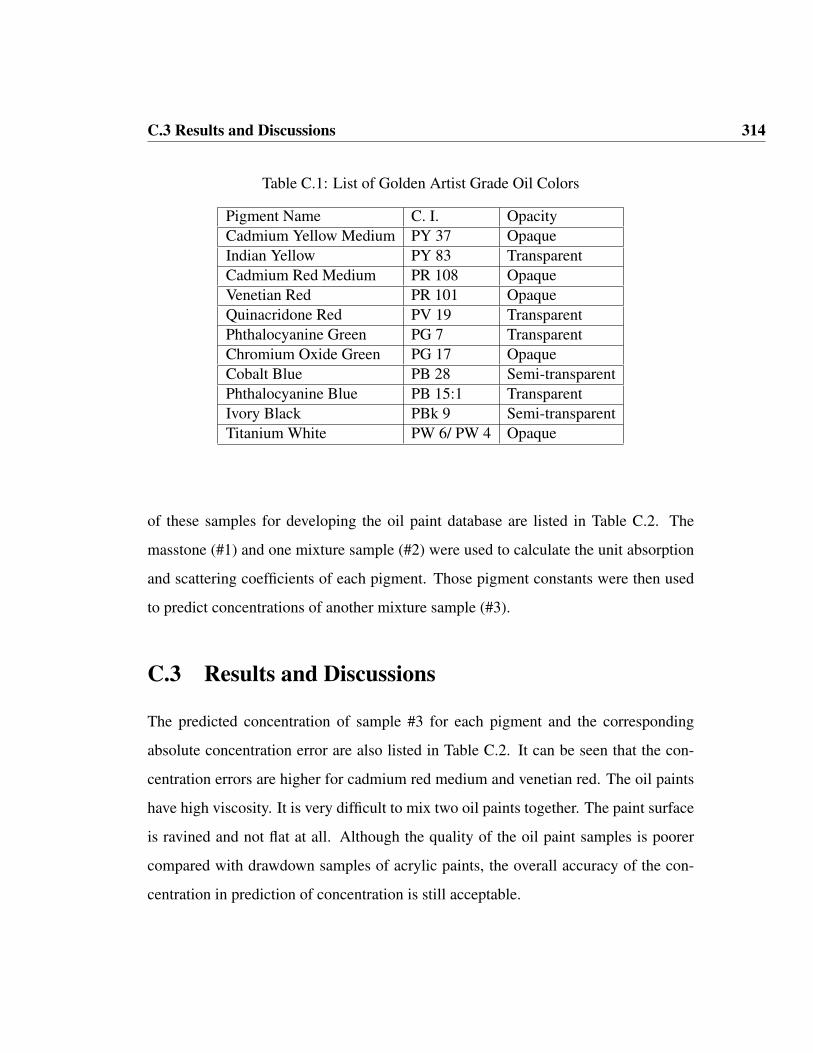
C.3 Results and Discussions 314
Table C.1: List of Golden Artist Grade Oil Colors
Pigment Name C. I. OpacityCadmium Yellow Medium PY 37 OpaqueIndian Yellow PY 83 TransparentCadmium Red Medium PR 108 OpaqueVenetian Red PR 101 OpaqueQuinacridone Red PV 19 TransparentPhthalocyanine Green PG 7 TransparentChromium Oxide Green PG 17 OpaqueCobalt Blue PB 28 Semi-transparentPhthalocyanine Blue PB 15:1 TransparentIvory Black PBk 9 Semi-transparentTitanium White PW 6/ PW 4 Opaque
of these samples for developing the oil paint database are listed in Table C.2. The
masstone (#1) and one mixture sample (#2) were used to calculate the unit absorption
and scattering coefficients of each pigment. Those pigment constants were then used
to predict concentrations of another mixture sample (#3).
C.3 Results and Discussions
The predicted concentration of sample #3 for each pigment and the corresponding
absolute concentration error are also listed in Table C.2. It can be seen that the con-
centration errors are higher for cadmium red medium and venetian red. The oil paints
have high viscosity. It is very difficult to mix two oil paints together. The paint surface
is ravined and not flat at all. Although the quality of the oil paint samples is poorer
compared with drawdown samples of acrylic paints, the overall accuracy of the con-
centration in prediction of concentration is still acceptable.

C.3 Results and Discussions 315
Table C.2: Recipes of paint samples used for the oil paint database
Concentrations (Mass, %)Pigment Name #1 #2 #3 #3 Pred. DifferenceCadmium Yellow Medium 100 51.0 20.0 22.5 2.5Indian Yellow 100 52.4 18.5 22.9 4.4Cadmium Red Medium 100 51.1 79.6 68.6 11.0Venetian Red 100 52.3 78.9 89.0 10.1Quinacridone Red 100 50.0 21.4 21.4 0.0Phthalocyanine Green 100 52.1 20.5 27.4 6.9Chromium Oxide Green 100 60.5 20.4 22.1 1.7Cobalt Blue 100 60.3 20.6 21.0 0.4Phthalocyanine Blue 100 59.7 20.3 27.1 6.8Ivory Black 100 59.2 19.6 24.7 5.1
In addition to prediction of concentration, the spectral and colorimetric accuracies
for these mixtures (#3) was quantified using three metrics in Table C.3. These met-
rics included RMS spectral error between measured and predicted reflectance factors,
color difference CIEDE2000 for CIE illuminant D65 and the 2-degree observer, and a
metameric index (M.I.) from D65 to CIE illuminant A. Both the spectral and colori-
metric performances were satisfactory.
Table C.3: Statistical results for spectral and colorimetric accuracies for the mixturesamples (#3)
Statistics RMS Error (%) Color Difference (∆E00) M.I. (∆E00, D65 → A)Average 1.1 1.0 0.1Std. Dev. 0.8 0.6 0.1Maximum 3.0 2.1 0.390% Percentile 2.4 1.9 0.3

C.4 Conclusions 316
C.4 Conclusions
The pigment constants of gamblin artist oil paints were characterized based on two
samples - one masstone and one mixture sample with whit paint. Then these pig-
ment constants were used to predicted the concentrations of other independent mixture
samples. Although the quality of the oil paint samples is poorer compared with the
drawdown samples of the acrylic paints, the accuracy of the predicted concentrations
is acceptable. The spectral and colorimetric accuracies of the predicted reflectance
factors are satisfactory.

Appendix D
PCA and ICA
D.1 Introduction
Reflectance spectra are generally smooth or band-limited, and can be represented by
a linear combination of several basis functions. Both principal component analysis
(PCA) and independent component analysis (ICA) will be used to find these basis
functions. These basis functions have be used in parameric decomposition for evalu-
ating metamerism (Li and Berns, 2007). The test data is the 1269 reflectance spectra
of the chips in the Munsell Book of Color-Matte Finish Collection. Three basis func-
tions are calculated for both PCA and ICA techniques. The reflectance spectra can be
reconstructed by a linear combinations of these basis functions with and without the
mean reflectance spectra. The reconstruction accuracies are compared between three
basis functions based upon PCA and ICA, and between with and without the mean
reflectance spectrum.

D.2 PCA 318
D.2 PCA
PCA is an effective technique used to reduce multidimensional data sets to lower di-
mensions for analysis. PCA involves the computation of the eigenvalue decomposition
or singular value decomposition of a data set. Eigenvectors and their corresponding
eigenvalues are calculated from the covariance matrix of the data set. The first eigen-
vector explains the most variability of the data set, and the second explains the second
most variability, and so on.
The reflectance spectra of a data set X is a a q-by-n matrix where q is the number
of samples and n is number of wavelengths. Each row of matrix X is a reflectance
spectrum Xi (i = 1, 2, . . . , q). The n-by-n covariance matrix C can be calculated
using Eq. (D.1), where X is a 1-by-n mean reflectance spectrum of the data set. Then
both the eigenvalues and eigenvectors are calculated based on the covariance matrix
C.
C =1
q − 1
q∑i=1
(Xi −X
)′ (Xi −X
)(D.1)
The first three eigenvectors or principal components (PCs) are used to reduce the
dimensionality of data set, and then to reconstruct the reflectance spectra from lower-
dimension data.
PCA Discarding the Mean The reflectance spectra can be represented with a linear
model Eq. (D.2), where E is a 3-by-n matrix, and each row is a 1-by-n eigenvector or
PC, ei (i = 1, 2, 3).
X = AE (D.2)

D.2 PCA 319
The q-by-3 matrix of loadings or scores, A, can be calculated in Eq. (D.3), where the
symbol † indicts the Moore-Penrose pseudo-inverse. The matrix A is a lower dimen-
sion representation of the original data set X. Since the eigenvectors are orthonormal
basis functions, i.e., eie′j = 1 when i = j, otherwise, eie
′j = 0, the multiplication
result of E and E′ is a 3-by-3 identity matrix.
A = XE†
= XE′ (EE′)−1
= XE′ (D.3)
Finally, the reflectance spectra can be reconstructed from the matrix A and three eigen-
vectors by substituting Eq. (D.3) in Eq. (D.2). The symbol means the estimated matrix
of the data set, in order to differentiate from the original data set X.
X = XE′E (D.4)
PCA Including the Mean The mean reflectance spectrum X is a 1-by-n vector, and
1 is a q-by-1 vector. The reflectance spectra can be expressed also as a linear combi-
nations of three eigenvectors or PCs plus the mean reflectance spectrum as shown in
Eq.(D.5).
X = AE + 1X (D.5)
The loading matrix A can be calculated from the centered data set, i.e., the mean
reflectance spectrum is subtracted from each and every reflectance in the data set, X−
1X.
A =(X− 1X
)E′ (D.6)

D.3 ICA 320
Then, the reflectance spectra can be reconstructed from three eigenvectors and the
mean reflectance spectrum again by substituting Eq. (D.6) in Eq. (D.5).
X =(X− 1X
)E′E + 1X (D.7)
D.3 ICA
The goal of ICA is to find basis functions that give rise to maximum statistical inde-
pendence of the data. Also take the spectral Munsell data as an example. In Eq. (D.8),
X is a q-by-n where q is the number of samples and n is number of wavelengths, A is
a q-by-m mixing matrix where m is number of independent basis functions, and S is
a m-by-n matrix of independent basis functions or independent components with each
row as a independent component.
X = AS (D.8)
The JADE (Joint Approximate Diagonalization of Eigenvalues) algorithm is used
to separate A and S from the data X. The output of the JADE algorithm is the separation
matrix B which is a m-by-q matrix. The matrix S can be calculated from B.
S = BX (D.9)
Then, the data can also be reconstructed from the separation matrix B and matrix
S where the symbol † represents the pseudo-inverse. Comparing Eq.(D.10) and Eq.

D.3 ICA 321
(D.8), it is found that the mixing matrix A is approximately equivalent to B†.
X = B†S (D.10)
D.3.1 Preprocessing Data
A first step in many ICA algorithms is to remove the mean from the data and whiten
(sphere) the data. This means that we remove any correlations in the data, i.e. the
signals are forced to be uncorrelated. The mean value of each reflectance is subtracted
from the reflectance spectrum, and the mean is a q-by-1 vector, represented by X. It
should be noted that this mean vector is not the mean reflectance spectrum as in PCA
and has no physical interpretation.
“Whitening” is done by a transformation matrix V such that when X = VX, the
correlation matrix E{XX′} = I (I is an identity matrix). This is easily accomplished
by setting V = C−1/2, where C = E{XX′} is the covariance matrix of the centered
data, since we have E{XX′} = E{VXX′V′} = C−1/2CC−1/2 = I.
However, “whitening” is generally performed via eigenvalue decomposition of co-
variance matrix C = E{XX′} = UDU′, where U is the orthogonal matrix of eigen-
vectors of the covariance matrix and D is the diagonal matrix of its eigenvalues. It is
worth mentioning that the covariance matrix is the same for the original data X and
the centered data X. Then, V = D−1/2U′. It will be extremely beneficial to reduce
the dimension. So the first k largest eigenvectors and the corresponding eigenvalues of
the covariance C are selected and the rest are discarded. The number of dimension is
reduced from q to k. Here are the abridged matrix D = diag (λ1, λ2, . . . , λk) (λi is a

D.3 ICA 322
scalar of eigenvalue) and the matrix U = [e1, e2, . . . , ek] (ei is a q-by-1 eigenvector).
The centered and whitened data X is a k-by-n matrix.
After the preprocessing of the data (i.e., centering and whitening), the separation
matrix B is obtained from the JADE algorithm. Then the independent basis functions
or S matrix can be calculated from Eq. (D.9).
D.3.2 Reconstruction Data
The reflectance spectra of the data set can also be reconstructed from the lower dimen-
sional data and three independent components in the same way as the discussion in
PCA. In order to compare with PCA, the mean reflectance spectrum is used here.
ICA Discarding the Mean The reflectance spectra is expressed as a linear model Eq.
(D.8), where S is a 3-by-n matrix, and each row is a 1-by-n independent components
si (i = 1, 2, 3). The q-by-3 mixing matrix, A, can be calculated in Eq. (D.11). The
matrix A is a lower dimension representation of X. Since the independent components
are not orthonormal as the eigenvectors, no further simplification can be done.
A = XS† (D.11)
Finally, the reflectance spectra can be reconstructed from the matrix A and three inde-
pendent components.
X = XS†S (D.12)
ICA Including the Mean The mean reflectance spectrum X is a 1-by-n vector, and 1
is a q-by-1 vector. The reflectance spectra can be represented as a linear combinations

D.4 Student’s t-Test 323
of three independent components plus the mean reflectance spectrum.
X = AS + 1X (D.13)
The mixing matrix A can be calculated from the centered data set.
A =(X− 1X
)S† (D.14)
Then, the reflectance spectra can be reconstructed from three independent components
and mean reflectance spectrum.
X =(X− 1X
)S†S + 1X (D.15)
D.4 Student’s t-Test
The reflectance spectra can be reduced to three dimensions using both PCA and ICA
techniques. After that, the reflectance spectra can be reconstructed from three eigen-
vectors with and without the mean reflectance spectrum, and from three independent
components with and without the mean reflectance spectrum. The spectral root-mean-
square (RMS) errors between the original and reconstructed data are calculated for all
four methods, and statistical t-test is used to do paired comparison among these four
methods.
Student’s t-test is one of the most commonly used techniques for testing a null
hypothesis H0 that two groups could have the same mean and alternative hypothesis
H1 that their means are different, where µ1 and µ2 are the means of these two groups.

D.4 Student’s t-Test 324
The underlining assumption of t-test is that these two samples should be normally
distributed. The spectral RMS errors between the original and reconstructed data sets
is approximately normally distributed.
H0 : µ1 = µ2 (D.16)
H1 : µ1 6= µ2 (D.17)
The statistical t value can be calculated from the means (µ1 and µ2), standard
derivations (s1 and s2), and numbers of the samples (n1 and n2) of these two groups.
The standard derivation of the two groups combined is obtained using Eq. (D.18),
and then the statistical t value can be calculated with Eq. (D.19). The degree of free-
dom (dof) is equal to number of samples in two groups combined minus two, i.e.,
dof = n1 + n2 − 2.
s =
√(n1 − 1)s2
1 + (n2 − 1)s22
n1 + n2 − 2(D.18)
t =|µ1 − µ2|
s√
1n1
+ 1n2
(D.19)
If the statistical t value is greater than the critical value at the significant level
α, the null hypothesis is rejected, otherwise, the alternative hypothesis is rejected.
The critical value can be obtained from the table of student’s t-distribution percentage
points for a given significant level and degree of freedom. Since student’s t distribution
is symmetric, the critical value at the significant level α for two tail is equal to the
critical value at 2α for one tail.

D.5 Results and Discussions 325
D.5 Results and Discussions
In this experimental, 1269 reflectance spectra of the chips in the Munsell Book of
Color-Matte Finish Collection are used as the data set. The wavelength range is from
380nm to 800nm with 1nm interval. For simplicity, the data is down-sampled, and the
new wavelength range is from 380nm to 800nm and 10nm intervals. So the number
of wavelengths n is 43, and the number of samples q is 1269. Three basis functions
for PCA and ICA calculated based upon the Munsell spectral data set are plotted in
Figures D.1 and D.2, respectively. Three basis functions of ICA were normalized, re-
ordered and changed signs. After that, three basis functions from ICA and PCA are
very similar.
Figure D.1: Three eigenvectors of the Munsell spectral data set from PCA

D.5 Results and Discussions 326
Figure D.2: Three independent components (ICs) of the Munsell spectral data set fromICA
Table D.1: Four spectral reconstruction methods
Method Basis Functions Mean Reflectance spectrumPCA Three PCs Disregarding
PCA+Mean Three PCs IncludingICA Three ICs Discarding
ICA+Mean Three ICs Including
The 43-dimensions of the Munsell data set is reduced to three-dimensions using
PCA with and without mean reflectance spectrum, and ICA with and without mean
spectrum, and then munsell data set is reconstructed using four different reconstruc-
tion methods, listed in Table D.1. The same three eigenvectors (PCs), in Figure D.1, are
used in both PCA and PCA+Mean methods, and the three independent components,
in Figure D.2, are used in both ICA and ICA+Mean methods. The reconstruction
accuracy is evaluated with both colorimetric accuracy metrics and spectral accuracy

D.5 Results and Discussions 327
Table D.3: Statistical results of reconstructed spectral data with three basis functionsof PCA plus the mean reflectance spectrum (PCA+Mean)
Statistics Mean Max 95 %Percentile Std. Dev.∆Eab 5.55 71.06 12.98 5.53∆E00 4.07 21.3 9.12 2.85RMS 2.32 14.67 4.98 1.51
wRMS 13.68 184.15 32.8 13.88MI (D65 → A) 0.84 7.85 2.48 0.81MI (A → D65) 1.2 6.74 2.93 0.89
metrics. Colorimetric accuracy metrics include the color difference ∆Eab and ∆E00,
and spectral accuracy metrics include the root-mean-square (RMS) error, the weighted
RMS error with inverse of measured reflectance, the metameric indices from D65 to A
and from A to D65.
Table D.2: Statistical results of reconstructed spectral data with three basis functionsof PCA
Statistics Mean Max 95% Percentile Std. Dev.∆Eab 5.83 74.77 17.00 6.42∆E00 3.65 21.79 7.72 2.37RMS 2.83 15.44 5.74 1.58
wRMS 19.33 193.97 37.36 13.88MI (D65 → A) 0.83 7.82 2.53 0.82MI (A → D65) 1.05 7.08 3.15 0.98
Tables D.2 and D.3 list statistical results of reconstruction accuracy using three
principal components with and without the mean reflectance spectrum. Tables D.4 and
D.5 list statistical results of reconstruction accuracy using three independent compo-

D.5 Results and Discussions 328
Table D.4: Statistical results of reconstructed spectral data with three basis functionsof ICA
Statistics Mean Max 95 %Percentile Std. Dev.∆Eab 5.44 72.54 14.5 5.82∆E00 3.82 21.32 8.92 2.67RMS 2.55 14.82 4.76 1.46
wRMS 15.3 185.35 32.55 13.47MI (D65 → A) 0.85 8.01 2.5 0.81MI (A → D65) 1.17 6.79 2.98 0.91
Table D.5: Statistical results of reconstructed spectral data with three basis functionsof ICA plus the mean reflectance spectrum (ICA+Mean)
Statistics Mean Max 95 %Percentile Std. Dev.∆Eab 5.38 72.54 14.61 5.87∆E00 3.76 21.35 8.77 2.68RMS 2.41 14.9 4.9 1.58
wRMS 13.93 186.94 33.81 14.16MI(D65→A) 0.84 7.99 2.48 0.82
MI (A → D65) 1.15 6.82 2.95 0.92

D.5 Results and Discussions 329
nents with and without the mean reflectance spectrum. It can be seen that the perfor-
mance including the mean reflectance spectrum for both ICA and PCA is better than
that discarding the mean. The performance of ICA is very difficult to compare with
that of PCA.
Student’s t-test is used to compare these four reconstruction methods based on the
spectral RMS error. The statistical t values for paired comparisons are listed in Table
D.6. Only the statistical t value between ICA+Mean and PCA+Mean is less than the
critical value 2.18 at the significant level 0.05, and the null hypothesis that two groups
have the same mean is rejected. Three principal components (PCs) and independent
components (ICs) are calculated based on the training data - the spectral Munsell data
set. Generally speaking, the mean reflectance spectrum of the training data is different
from the mean reflectance spectrum of other testing data sets. So the reconstruction
methods of PCA and ICA are better than those of PCA+Mean and ICA+Mean when
the mean reflectance spectra for other independent testing data are unavailable. The
t-value for PCA and ICA is 4.79, greater than the critical value, so their mean RMS
errors are significantly different from each other. The mean RMS error for ICA is a
little smaller than that for PCA. Thus, three independent components of ICA are better
choice to reduce the dimensionality of data set and to parameric decomposition.
Table D.6: Paired comparisons of the four different reconstruction methods
PCA PCA+Mean ICA ICA+MeanPCA 0 8.3604 4.7892 6.7456
PCA+Mean 8.3604 0 3.7927 1.4433ICA 4.7892 3.7927 0 2.2273
ICA+Mean 6.7456 1.4433 2.2273 0

D.6 Conclusions 330
D.6 Conclusions
PCA is an effective technique to reduce the dimensionality of the data set. Three basis
functions of PCA are calculated based upon the eigenvalue decomposition of the co-
variance matrix of the data set. The purpose of ICA is to find basis functions that give
rise to maximum statistical independence of the data. Three basis function of ICA are
calculated based upon JADE algorithm, and the data should be preprocessed (centering
and whitening) first. After that, the data can be reduced to lower dimension using four
different methods (PCA, PCA+Mean, ICA and ICA+Mean) and reconstructed again.
The statistical results of the reconstruction accuracy are discussed in detail. Although
the performances of both PCA+Mean and ICA+Mean are better than the correspond-
ing methods discarding the mean reflectance spectrum for the training data, these two
methods are not useful for the other independent test data sets. The performance of
ICA is a little better than that of PCA. So, three independent components of ICA are a
better choice to reduce the dimensionality of data set and for parameric decomposition.

Bibliography
Allen, E. (1966). Basic equations used in computer color matching. J. Opt. Soc. Am.,
56(9):1256–1259.
Allen, E. (1974). Basic equations used in computer color matching, II. tristimulus
match, two-constant theory. J. Opt. Soc. Am., 64(7):991–993.
Allen, E. (1980). Chapter 7 Colorant formulation and shading, Optical Radiation
Measurements, volume 2. Academic Press.
Attas, M., Cloutis, E., Collins, C., Goltz, D., Majzels, C., Mansfield, J., and Mantsch,
H. (2003). Near-infrared spectroscopic imaging in art conservation: investigation
of drawing constituents. Journal of Culture Heritage, 4:127–136.
Attas, M., Mansfield, J., Majzels, C., Cloutis, E., Collins, C., and Mantsch, H. (2002).
Near-infrared spectroscopic reflectance imaging: a new tool in art conservation.
Vibration Spectroscopy, 28:59–66.
Baronti, S., Casini, A., Lotti, F., and Porcinai, S. (1998). Multispectral imaging sys-
tem for the mapping of pigments in works of art by use of principal-component
analysis. Applied Optics, 37:1299–1309.

BIBLIOGRAPHY 332
Bayerer, F. and Burmester, A. (1994). Non-destructive imaging spectroscopy of draw-
ings and paintings. In proceedings of the 18th International Symposium on the
Conservation and Restoration of Cultural Property, pages 76–85, Tokyo, Japan.
Berns, R. (1997). A generic approach to color modeling. Color Research and Appli-
cation, 22(5):318–325.
Berns, R. (2000). Billmeyer and Saltzmans Principles of Color Technology. John
Wiley and Sons, third edition.
Berns, R. (2005a). Color accurate image archives using spectral imaging. In Pro-
ceedings of (Sackler NAS Colloquium) Scientific Examination of Art: Modern
Techniques in Conservation and Analysis, pages 105–119. National Academies
Press.
Berns, R. (2005b). Rejuvenating the appearance of cultural heritage using color and
imaging science techniques. In Proceedings of the 10th Congress of the Interna-
tional Colour Association AIC Colour 05, pages 369–374, Granada, Spain. IS&T.
Berns, R., Byrns, S., Casadio, F., Fiedler, I., Gallagher, C., Imai, F., Newman, A., and
Taplin, L. (2006). Rejuvenating the color palette of george seurat’s A Sunday on
La Grande Jatte - 1884: a simulation. Color Res. & Appl., 31:278–293.
Berns, R. and de la Rie, R. (2003). The effect of a varnish’s refractive index on the
appearance of oil paintings. Studies in Conservation, 48:251–262.
Berns, R. and Imai, F. (2001). Pigment identification of artist materials via multi-
spectral imaging. In Proceedings of the IS&T/SID Ninth Color Imaging Confer-
ence, pages 85–90, Springfield, VA. IS&T.

BIBLIOGRAPHY 333
Berns, R. and Imai, F. (2002). The use of multi-spectral imaging for pigment iden-
tification. In Proceedings of the13th Triennial Meeting, ICOM Committee for
Conservation, pages 217–222, Rio de Janeiro. ICOM.
Berns, R., Imai, F., Burns, P., and Tzeng, D. (1998). Multispectral-based color repro-
duction research at the munsell color science laboratory. In International Society
for Optical Engineering, volume 3409, pages 14–25, Bellingham, Washington.
Berns, R. and Katoh, N. (2002). Methods of Characterizing Displays, Color Engi-
neering: Achieving Device Independent Colour, edited by P. Green and L. W.
MacDonald, pages 127–164. John Wiley & Sons, England.
Berns, R., Krueger, J., and Swicklik, M. (2002). Multiple pigment selection for in-
painting using visible reflectance spectrophotometry. Studies in Conservation,
47:46–61.
Berns, R. and Mohammadi, M. (2007a). Evaluating single- and two-constant kubelka-
munk turbid media theory for instrumental-based inpainting. Studies in Conser-
vation, 52:299–314.
Berns, R. and Mohammadi, M. (2007b). Single-constant simplification of kubelka-
munk turbid-media theory for paint systems - a review. Color Research & Appli-
cation, 32:201–207.
Berns, R., Taplin, L., Nezamabadi, M., Mohammadi, M., and Zhao, Y. (2005a). Spec-
tral imaging using a commercial color filter array digital camera. In Proceedings
of the 14th Triennial ICOM-CC Meeting, pages 743–750, Hague, Netherlands.
ICOM.

BIBLIOGRAPHY 334
Berns, R., Taplin, L., Nezamabadi, M., Zhao, Y., and Okumura, Y. (2005b). High-
accuracy digital imaging of culture heritage without visual editing. In Proceedings
of IS&T Archiving Conference, pages 91–95, Springfield, VA. IS&T.
Berrie, B. (1992). Understanding art through technical analysis inferences from pig-
ment identification. In Mat. Res. Soc. Symp., volume 267, pages 195–204.
Best, S., Clark, R. J., Daniels, A., Porter, C., and Withnall, R. (1995). Identifica-
tion by raman microscopy and visible refelctance spectroscopy of pigments on an
icelandic manuscript. Studies in Art Conservations, 40:31–40.
Billmeyer, F., Saltzman, J. M., and Kumar, R. (1982). Identification of organic pig-
ments by solution spectrophotometry. Color Research and Application, 7:327–
337.
Billmeyer, F. J., Chassaigne, P., and JF, J. D. (1980). Determining pigment optical
properties for use in the mie and many-flux theories. Color Res. Appl., 5:108112.
Burmester, A., Bayerer, F., and Munchen (1994a). Remote imaging spectroscopy of
drawings. In Proceedings of the 4th International Conference: Non-destructive
Testing of Works of Arts, pages 183–192, Berlin.
Burmester, A., Wei, W., and Munchen (1994b). All good paintings crack: non-
destructive analysis of transport damage of paintings using digital image process-
ing. In Proceedings of the 4th International Conference: Non-destructive Testing
of Works of Arts, pages 114–124, Berlin.
Burns, P. and Berns, R. (1996). Analysis of multispectral image capture. In Proceed-
ings of the IS&T/SID Fourth Color Imaging Conference Color Science, Systems,
and Applications, pages 19–22, Springfield, VA. IS&T.

BIBLIOGRAPHY 335
Cairns, E., Holtzen, D., and Spooner, D. (1976). Determining absorption and scattering
constants for pigments. Color Research and Application, 1:174–180.
Casini, A., Lotti, F., Picollo, M., Stefani, L., and Buzzegoli, E. (1999). Image spec-
troscopy mapping technique for non-invasive analysis of painting. Studies in Con-
servation, 44:39–48.
Chong, P., Edwin, K., and Stanislaw, H. (2001). An introduction to optimization. John
Wiley & Sons, second edition.
Ciliberto, E. and Spoto, G. (2000). Modern analytical methods in art and archaeology.
John Wiley & Sons, first edition.
Clark, R., Gallagher, A., Gregg, A., Swayze, and Vergo, N. (1990). Material absorption
band depth mapping of imaging spectrometer data using a complete band shape
least-squares fit with library reference spectra. In Green, R. O., editor, AVIRIS
Workshop, pages 176–186.
Clark, R. and Roush, T. (1984). Reflectance spectroscopy: quantitative analysis
techniques for remote sensing applications. Journal of Geophysical Research,
89(B7):6329–6340.
Cogno, J. (1998). Recursive quadratic programming algorithm for color matching.
Color Research & Application, 13:124–126.
Cogno, J., Jungman, D., and Conno, J. (1998). Linear and quadratic optimization
algorithms for computer color matching. Color Research & Application, 13:40–
45.

BIBLIOGRAPHY 336
Cohen, J. (1988). Color and color mixture: Scalar and vector fundamentals. Color
Research & Application, 13:5–39.
Cohen, J., editor (2001). Visual Color and Color Mixture: The Fundamental Color
Space. University of Illinois Press, Urbana, IL.
Cohen, J. and Kappauf, W. (1982). Metameric color stimuli, fundamental metamers,
and wyszeckis metameric blacks. Am. J. Psycho., 95:537–564.
Cohen, J. and Kappauf, W. (1985). Color mixture and fundamental metamers: Theory,
algebra, geometry, application. Am. J. Psycho., 98:171–259.
Davidson, H. and Hemmendinger, H. (1966). Color prediction using the two-constant
turbid-media theory. J. Opt. Soc. Am., 56:1102–1109.
Davison, H. and Hemendinger, H. (1966). Color prediction using the two-constant
turbid-media theory. J. Opt. Soc. Am., 56(8):1102–1109.
Derby, R. (1952). Applied spectrophotometry i. color matching with the aid of the r
cam. American Dyestuff Reporter, 41:550–557.
Derhak, M. and Rosen, M. (2004). Spectral colorimetry using labpqr - an interim
connection space. In Proceedings of the 12th Color Imaging Conference, pages
246–250, Springfield, VA. IS&T.
Duda, R., Hart, P., and Stork, D. (2001). Pattern Classification. John Wiley & Sons,
second edition.
Duncan, D. (1949). The colour of pigment mixtures. J. Oil Colour Chem. Assoc.,
32:296.

BIBLIOGRAPHY 337
Fairman, H. (1987). Metameric correction using parametric decomposition. Color
Research & Application, 12:261–265.
Fairman, H. (1991). Recommended terminology for matrix r and metamerism. Color
Research & Application, 16:337–341.
Foody, G., Lucas, R., Curran, P., and Honzak, M. (1997). Nonlinear mixture modeling
without end-members using an artificial neural network. Int. J. Remote Sensing,
18:937–953.
Gross, H. and Schott, J. (1996). Application of spatial resolution enhancement and
spectral mixing analysis to hyperspectral images. In Proceedings of SPIE Optical
Science, Engineering and Instrument Annual Meeting, volume 2821-4, pages 30–
41, Denver, Colorado. IS&T.
Gross, H. and Schott, J. (1998). Application of spectral mixture analysis and image
fusion techniques for image sharpening. Remote Sens. Environ., 63:85–94.
G.Wyszecki (1953). Valenzmetrische undersuchung des zusammenhanges zwischen
normaler und anomaler trichromasie, (psychophysical investigation of relation-
ship between normal and abnormal trichromatic vision). Farbe, 2:39–52.
Hardeberg, J. (1999). Acquisition and reproduction of color images: colorimet-
ric and multispectral approaches. PhD thesis, Ecole Nationale Superieure des
Telecommunications, ENST, Paris, France.
Hardeberg, J., Schmitt, F., and Brettel, H. (2002). Multispectral color image capture
using a liquid crystal tunable filter. Opt. Eng., 41:2532–2548.
BIBLIOGRAPHY 338
Helling, S. and Seidel, E. (1998). Algorithms for spectral color stimulus reconstruction
with a seven-channel multispectral camera. In Proceedings of CGIV: the 2nd
European Conference on Color Graphics, Imaging and Vision, pages 254–258.
IS&T.
Herzog, P., Knip, D., Stiebig, H., and Konig, F. (1999). Colorimetric characterization
of novel multiple-channel sensors for imaging and metrology. J. of Electronic
Imaging, 8(4):342–353.
Hill, B. (1998). Multispectral color technology: a way towards high definition color
image scanning and encoding. In Proceedings of SPIE 3409: Electronic Imaging:
Processing, Printing and Publishing in Color, pages 2–13, Zurich, Switzerland.
Hoffenberg, P. (1972). Automated color-match of printed ink films. PhD thesis, Lehigh
University, Bethlehem,PA.
Imai, F. and Berns, R. (1998). High-resolution multi-spectral image archives: A hybrid
approach. In Proceedings of the 6th Color Imaging Conference: Color Science,
Systems and Applications, pages 224–227, Springfield, VA. IS&T.
Imai, F., Berns, R., and Tzeng, D. (2000a). A comparative analysis of spectral re-
flectance estimation in various spaces using a trichromatic camera system. J. of
Imag. Sci. Tech., 44:280–287.
Imai, F., Rosen, M., and Berns, R. (2000b). Comparison of spectrally narrow-band
capture versus wide-band with a priori sample analysis for spectral reflectance
estimation. In Proceedings of the 8 th Color Imaging Conference, pages 234–
241, Springfield, VA. IS&T.
BIBLIOGRAPHY 339
Imai, F., Rosen, M., and Berns, R. (2002a). Comparative study of metrics for spectral
match quality. In Proceedings of the 1st European Conference on Color in Graph-
ics, CGIV2002, Imaging and Vision, pages 492–496, Springfield, VA. IS&T.
Imai, F., Taplin, L., and Day, E. (2002b). Comparison of the accuracy of various
transformations from multi-band images to reflectance spectra. Technical report,
Munsell Color Science Lab.
Imai, F., Taplin, L., and Day, E. (2003). Comparative study of spectral reflectance es-
timation based on broad-band imaging systems. Technical report, Munsell Color
Science Lab.
Johnson, R. and Wichern, D. (2001). Applied multivariate statistics analysis. Prentice-
Hall, Inc., fifth edition.
Johnston, R. and Feller, R. (1963). The use of differential spectral curve analysis in
the study of museum objects. Dyestuffs, 44:1–10.
Joshi, J., Vaidya, D., and Shah, H. (2001). Application of multi-flux theory based on
mie scattering to the problem of modeling the optical characteristics of colored
pigmented paint films. Color Res. Appl., 26:234:245.
Judd, D. and Wyszecki, G. (1975). Color in Business, Science and Industry. John
Wiley & Sons, 3rd edition.
Keusen, T. (1996). Multispectral color system with an encoding format compatible
with conventional tristimulus model. J. of Imag. Sci. Tech., 40(6):510–515.
Konig, F. and Herzog, P. G. (1999). On the limitation of metameric imaging. In
Proceedings of the IS&Ts PICS conference, pages 163–166.

BIBLIOGRAPHY 340
Konig, F. and Praefcke, W. (1998). The practice of multispectral image acquisition.
In Proceedings of SPIE3409: Electronic Imaging: Processing, Printing and Pub-
lishing in Color, volume 3409, pages 34–41. SPIE.
Kubelka, P. (1948). New contributions to the optics of intesnsely light-scallering ma-
terials, part i. J. Opt. Soc. Am., 38(5):448–457, 1067.
Kubelka, P. (1954). New contributions to the optics of intensely light-scattering mate-
rials, part ii: Nonhomogeneous layers. J. Opt. Soc. Am., 44:330–335.
Kubelka, P. and Munk, F. (1931). Ein beitrag zur optik der farbanstriche. Zeritschrift
fr technische Physik, 12:593–601.
Laamanen, H., Jaaskelainen, T., Hauta-Kasari, M., Parkkinen, J., and Miyata, K.
(2004). Imaging spectrograph based spectral imaging system. In Proceedings
of CGIV: the 2nd European Conference on Color Graphics, Imaging and Vision,
pages 427–430.
Learner, T. (2004). Analysis of modern paints (research in conservation technical
report series). Technical report, Getty Conservation institution.
Leona, M. and Winter, J. (2001). Fiber optics reflectance spectroscopy: a unique tool
for investigation of japanese paintings. Studies in Conservation, 46:153–162.
Li, Z. and Berns, R. (2007). Comparison of methods of parameric correction for eval-
uating metamerism. Color Research & Application, 32(4):293–303.
Liang, H., Saunders, D., and Cupitt, J. (2005). A new multispectral imaging system
for examining paintings. J. Imag. Sci. Tech., 49:551–562.

BIBLIOGRAPHY 341
Martinez, K., Cupitt, J., Saunders, D., and Pillay, R. (2002). Ten years of art imaging
research. In Proceedings of The IEEE, volume 90, pages 28–41.
McCabe, C. and Glinsman, L. (1995). Understanding alfred stieglitz platinum and
palladium prints: examination by x-ray fluorescence spectrometry. Studies in the
History of Art, 51:71–85.
McDonald, R., editor (1987). Colour physics for industry, pages 186–210. Society of
Dyers & Colourists, 1st edition.
Mehta, K. and Shah, H. (1987). Simplified equations to calculate mie-theory parame-
ters for use in many-flux calculations for predicting the reflectance of paints films.
Color Res. Appl., 12:147–155.
Miyake, Y., Yokoyama, Y., Tsumura, N., Haneishi, H., Miyake, K., and Hayashi, J.
(1999). Development of multiband color imaging system fro recordings of art
paintings. In Proceedings of SPIE 3648, volume 3648, pages 218–225.
Mohammadi, M. and Berns, R. (2004). Verification of the kubelka-munk turbid media
theory for artist acrylic paint. Technical report, Munsell Color Science Labora-
tory.
Mohammadi, M., Nezamabadi, M., Berns, R., and Taplin, L. (2004a). Spectral imaging
target development based on hierarchical cluster analysis. In Proceedings of the
12th Color Imaging Conference, pages 59–64, Springfield, VA. IS&T.
Mohammadi, M., Nezamabadi, M., Berns, R., and Taplin, L. (2005). A prototype
calibration target for spectral imaging. In Proceedings of the 10th Congress of the
International Colour Association, pages 387–390, Granada, Spain. IS&T.

BIBLIOGRAPHY 342
Mohammadi, M., Nezamabadi, M., Taplin, L., and Berns, R. (2004b). Pigment se-
lection using kubelka-munk turbid media theory and non-negative least square
technique. Technical report, Munsell Color Science Laboratory.
Mudget, P. and Richard, L. (1971). Multiple scattering calculations for technology.
Appl. Opt., 10:1485–1502.
Neter, J., Wasserman, W., and Kutner, M. (1996). Applied linear regression models.
McGraw-HillIrwin, third edition.
Nobbs, J. (1985). Kubelka-munk theory and the prediction of reflectance. Rev. Prog.
Coloration, 15:66–75.
Nobbs, J. (1997). Colour physics for industry: Chapter 6 Colour-match prediction for
pigmented materials. Society of Dyers and Colourists, second edition.
Okumura, Y. (2005). Developing a spectral and colorimetric database of artist paint
materials. Master’s thesis, Rochester institution of Technology.
Praefcke, W. (1996). Transform coding of reflectance spectra using smooth basis vec-
tors. J. of Imag. Sci & Tech., 40(6):543–548.
Pratt, W. and Mancill, C. (1976). Spectral estimation techniques for the spectral cali-
bration of a color image scanner. Applied Optics, 15(1):73–75.
Renger, K. and Burmester, A. (1986). The munich rembrandt forgeries reconsidered:
a new technical approach to the investigation of drawings. Master Drawings,
23/24:526–537.
BIBLIOGRAPHY 343
Ribes, A. and Schmitt, F. (2003). A fully automatic method for reconstruction of spec-
tral reflectance curves by using mixture density networks. Pattern Recognition
Letters, 24(11):1691–1701.
Ribes, A., Schmitt, F., Pillay, R., and Lahanier, C. (2005). Calibration and spectral
reconstruction for crisatel: An art painting multispectral acquisition system. J.
Imag. Sci. Tech., 49:563–573.
Robinson, G., Gross, H., and Schott, J. (2000). Evaluation of two applications of
spectral mixing models to imaging fusion. Remote Sensing Environment, 71:272–
281.
Rodrıguez, J. and Fernandez, J. (2005). Application of the second derivative of
the kubelka-munk function to the semi-quantitative analysis of roman paintings.
Color Research and Application, 30:448–456.
Ross, W. (1967). Kubelka-munk formulas adapted for better computation. J. Paint
Tech., 39:511–515.
Ryde, J. (1931). The scattering of light by turbid media part i. In Proceedings of Royal
Society, volume A131, pages 451–464.
Saunderson, J. (1942). Calculation of the color of pigmented plastics. J. Opt. Soc. Am.,
32:727–736.
Schmitt, F., Brettel, H., and Hardeberg, J. (1999). Multispectral imaging development
at enst. In Proceedings of International Symposium on Multispectral Imaging and
Color Reproduction for Digital Archives, pages 50–57, Chiba, Japan.
Sharma, G. (2003). Digital Color Imaging Handbook, chapter 1, page xx. CRC press.

BIBLIOGRAPHY 344
Shurcliff, A. (1942). Curve shape index for identification by means of spectrophoto-
metric curves. J. Opt. Soc. Am., 32:160–163.
Sluban, B. (1993). Comparison of colorimetric and spectrophotometric algorithms for
computer match prediction. Color Research & Application, 18:74–79.
Staniforth, S. (1985). Retouching and colour matching: the restorer and metamerism.
Studies in Conservation, 30:101–111.
Sugiura, H., Kuno, T., Watanabe, N., Matoba, N., Hayachi, J., and Miyake, Y. (2000).
Development of a multispectral camera system. In Proceedings of SPIE 3965:
Sensors and Camera Systems for Scientific, Industrial and Digital Photographic
Applications, volume 3965, pages 331–339.
Taplin, L. and Berns, R. (2005). Practical spectral capture systems for museum imag-
ing. In Proceedings of the 10th Congress of the International Colour Association
AIC Colour 05, pages 1287–1290, Granada, Spain.
Tennent, N., Nobbs, J., Binns, M., and Lawton, S. (2005). The use of computer-
match colour prediction in the restoration of ceramics. In Proceedings of the 14th
Triennial ICOM-CC Meeting, pages 146–153, Hague, Netherlands.
Thoma, J., Cupitt, J., and Saunders, D. (2000). An investigation of the potential use
of visible-region multispectral imaging for pigment identification in paintings. In
Proceedings of Color Image Science 2000, pages 95–106, Color & Image Insti-
tute, Univ. of Derby.
Thornton, W. (1991). A critique of recommended terminology for matrix r and
metamerism by hugh s. fairman. Color Research & Application, 16:361–363.

BIBLIOGRAPHY 345
Tominaga, S. (1996). Multichannel vision system for estimation surface and illumina-
tion functions. J. of Opt. Soc. Am. A, 13(11):2163–2173.
Tominaga, S. (1999). Multichannel cameras and spectral image processing. In Pro-
ceedings of international Symposium on Multispectral Imaging and Color Repro-
duction for Digital Archives, pages 18–25, Chiba, Japan.
Tominaga, S., Tanaka, N., and Matsumoto, T. (2002). Recording and rendering for art
paintings based on multiband data. In Proceedings of SPIE 4663, pages 27–34.
Tzeng, D. (1999). Spectral-based color separation algorithm development for
multiple-ink color reproduction. PhD thesis, Rochester Institute of Technology,
Rochester, NY.
Volz, H. G. (2001). Industrial Color Testing: Fundamentals and Techniques, Trans-
lated by Ben Teague. Wiley-VCH, Germany, second, completely revised edition.
Walmsley, E., Metzger, C., Delaney, J., and Fletcher, C. (1994). Improved visualization
of underdrawing with solid-state detectors operating in the infrared. Studies in
Conservation, 39:217–231.
Walowit, E., McCarthy, C., and Berns, R. (1988). Spectrophotometric color match-
ing based on two-constant kubelka-munk theory. Color Research & Application,
13:358–362.
Whitemore, P. (2002). Contributions to conservation science: a collection of Robert
Fellers published works on artists paints, paper, and varnishes. Carnegie-Mellon
University Press.

BIBLIOGRAPHY 346
Zhao, Y., Berns, R., Okumura, Y., and Taplin, L. (2005a). Improvement of spec-
tral imaging by pigment mapping. In Proceedings of the IS&T/SIDs 13th Color
Imaging Conference: Color Science and Engineering, Systems, Technologies and
Applications, pages 40–45, Scottsdale, Arizona.
Zhao, Y., Berns, R., and Taplin, L. (2006). Image segmentation and pigment mapping
in spectral imaging. In Proceedings of the 6th International Congress of Imaging
Science, pages 294–297, Rochester, New York.
Zhao, Y. and Berns, R. S. (2006). Development of colorant database for two-constant
kubelka-munk theory. Technical report, Munsell Color Science Laboratory.
Zhao, Y. and Berns, R. S. (2007). Image-based spectral reflectance reconstruction
using the matrix R method. Color Research & Application, 32(5):343–351.
Zhao, Y., Taplin, L., Nezamabadi, M., and Berns, R. (2005b). Using matrix R method
in the multispectral image archives. In Proceedings of the 10th Congress of the
International Colour Association AIC Colour 05, pages 469–472, Granada, Spain.