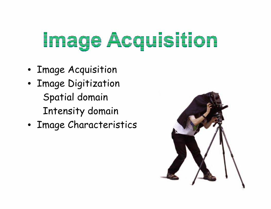
• Image Acquisition

• Image Digitization

Spatial domain

Intensity domain

• Image Characteristics

1

2

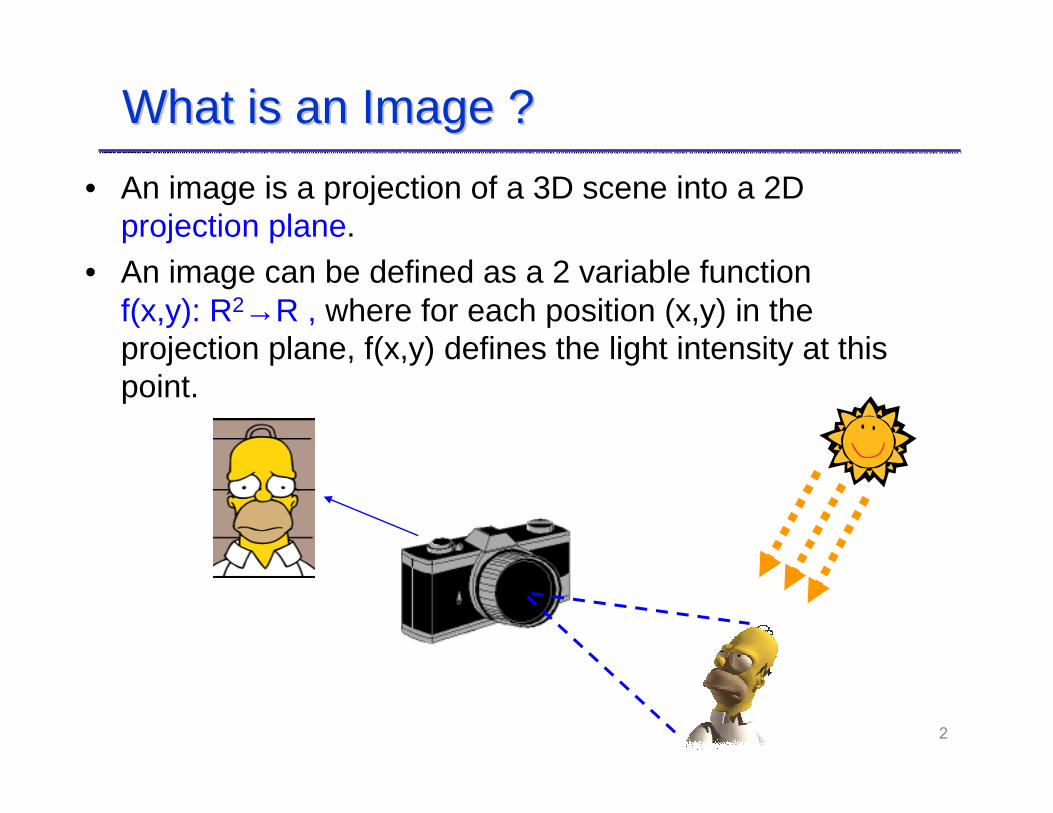
What is an Image ?What is an Image ?

• An image is a projection of a 3D scene into a 2D projection plane.

• An image can be defined as a 2 variable function f(x,y): R2→R , where for each position (x,y) in the projection plane, f(x,y) defines the light intensity at this point.

Image as a functionImage as a function

3

4

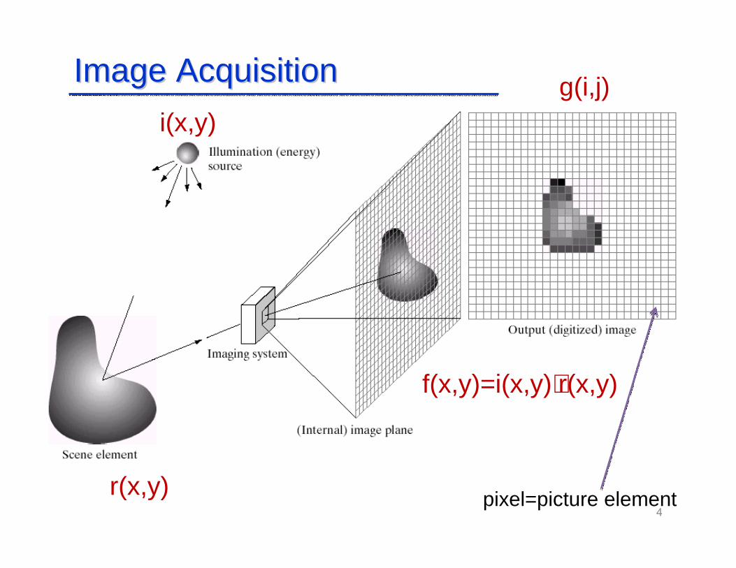
i(x,y)

r(x,y)

f(x,y)=i(x,y)⋅r(x,y)

g(i,j)Image AcquisitionImage Acquisition

pixel=picture element

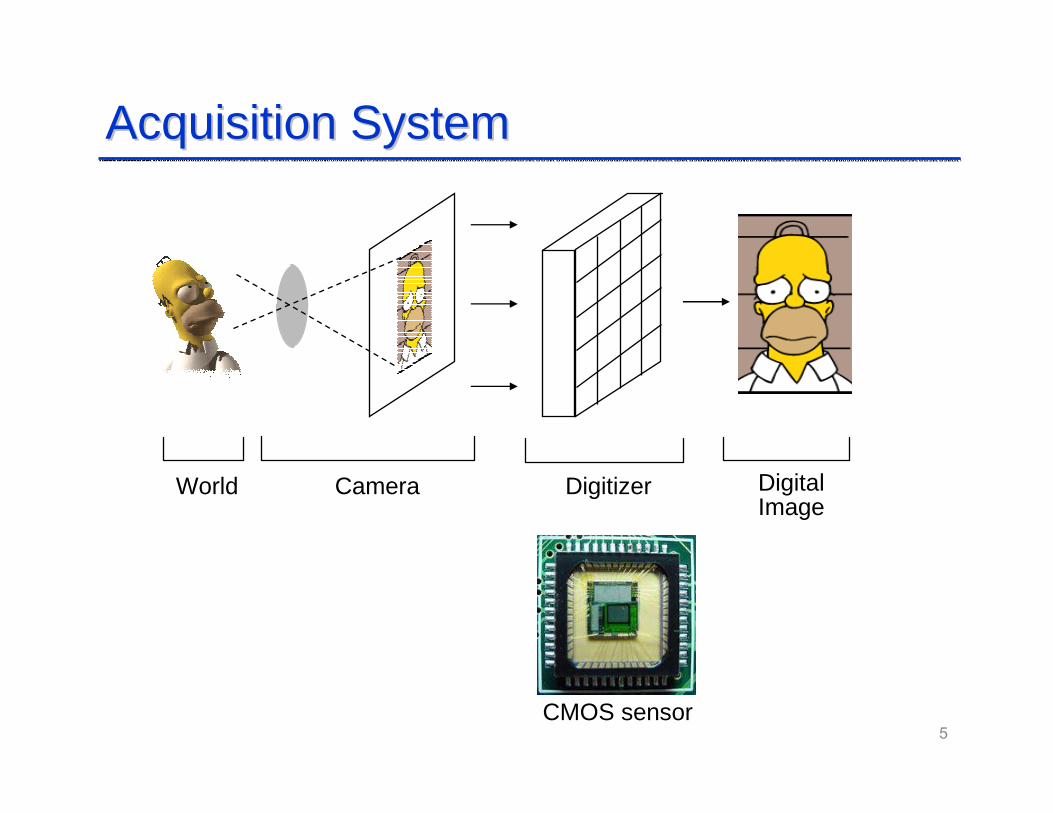
Acquisition SystemAcquisition System

5

World Camera Digitizer DigitalImage

CMOS sensor

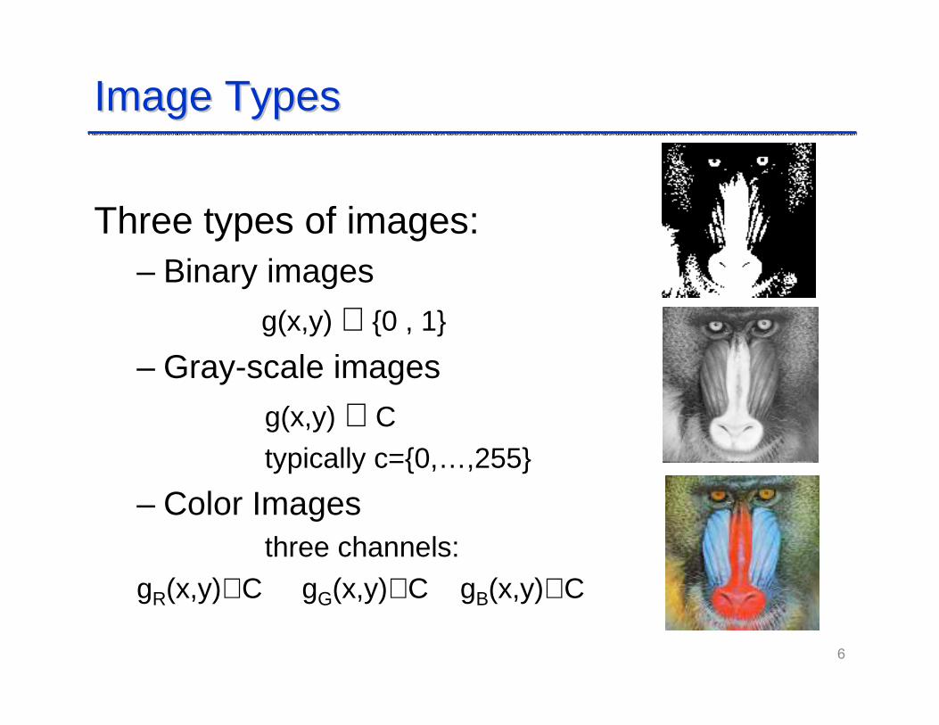
Image TypesImage Types

Three types of images:– Binary images

g(x,y) ∈ {0 , 1}

– Gray-scale images

g(x,y) ∈ C

typically c={0,…,255}

– Color Images three channels:

gR(x,y)∈C gG(x,y)∈C gB(x,y)∈C

6

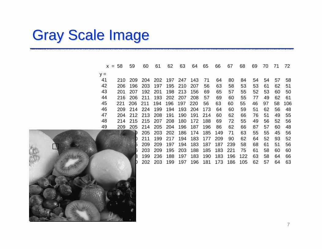
Gray Scale ImageGray Scale Image

7

210 209 204 202 197 247 143 71 64 80 84 54 54 57 58 206 196 203 197 195 210 207 56 63 58 53 53 61 62 51 201 207 192 201 198 213 156 69 65 57 55 52 53 60 50 216 206 211 193 202 207 208 57 69 60 55 77 49 62 61 221 206 211 194 196 197 220 56 63 60 55 46 97 58 106 209 214 224 199 194 193 204 173 64 60 59 51 62 56 48 204 212 213 208 191 190 191 214 60 62 66 76 51 49 55 214 215 215 207 208 180 172 188 69 72 55 49 56 52 56 209 205 214 205 204 196 187 196 86 62 66 87 57 60 48 208 209 205 203 202 186 174 185 149 71 63 55 55 45 56 207 210 211 199 217 194 183 177 209 90 62 64 52 93 52 208 205 209 209 197 194 183 187 187 239 58 68 61 51 56 204 206 203 209 195 203 188 185 183 221 75 61 58 60 60200 203 199 236 188 197 183 190 183 196 122 63 58 64 66 205 210 202 203 199 197 196 181 173 186 105 62 57 64 63

x = 58 59 60 61 62 63 64 65 66 67 68 69 70 71 72

y = 414243444546474849505152535455

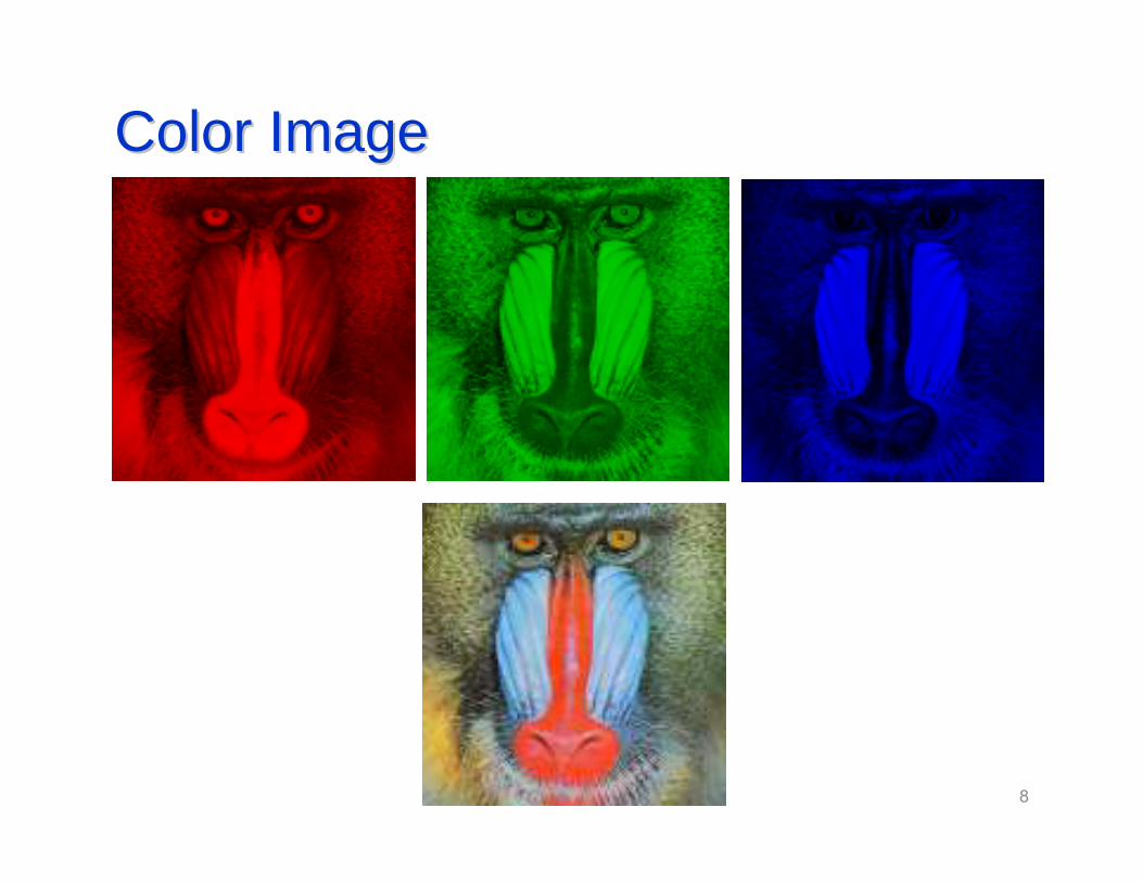
Color ImageColor Image

8

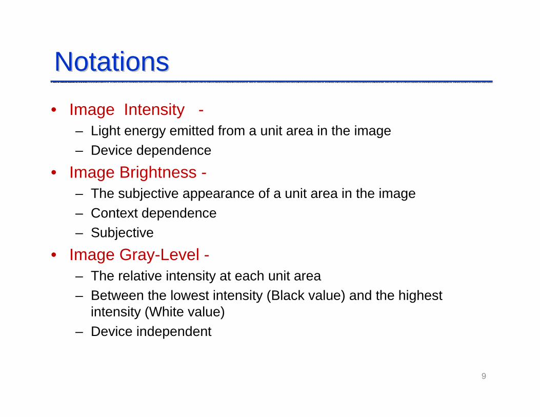
NotationsNotations

• Image Intensity -– Light energy emitted from a unit area in the image– Device dependence

• Image Brightness -– The subjective appearance of a unit area in the image– Context dependence– Subjective

• Image Gray-Level -– The relative intensity at each unit area– Between the lowest intensity (Black value) and the highest

intensity (White value)– Device independent

9

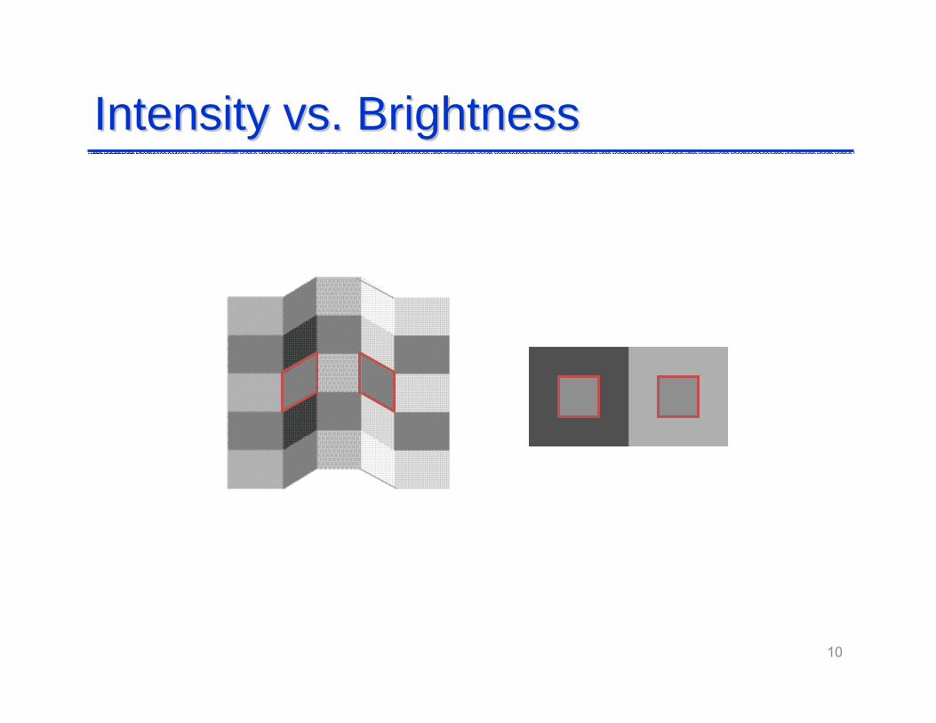
Intensity vs. BrightnessIntensity vs. Brightness

10

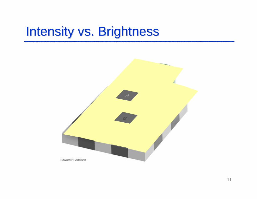
Intensity vs. BrightnessIntensity vs. Brightness

11

12

Inte

nsity

∆f1

∆f2f2

f1

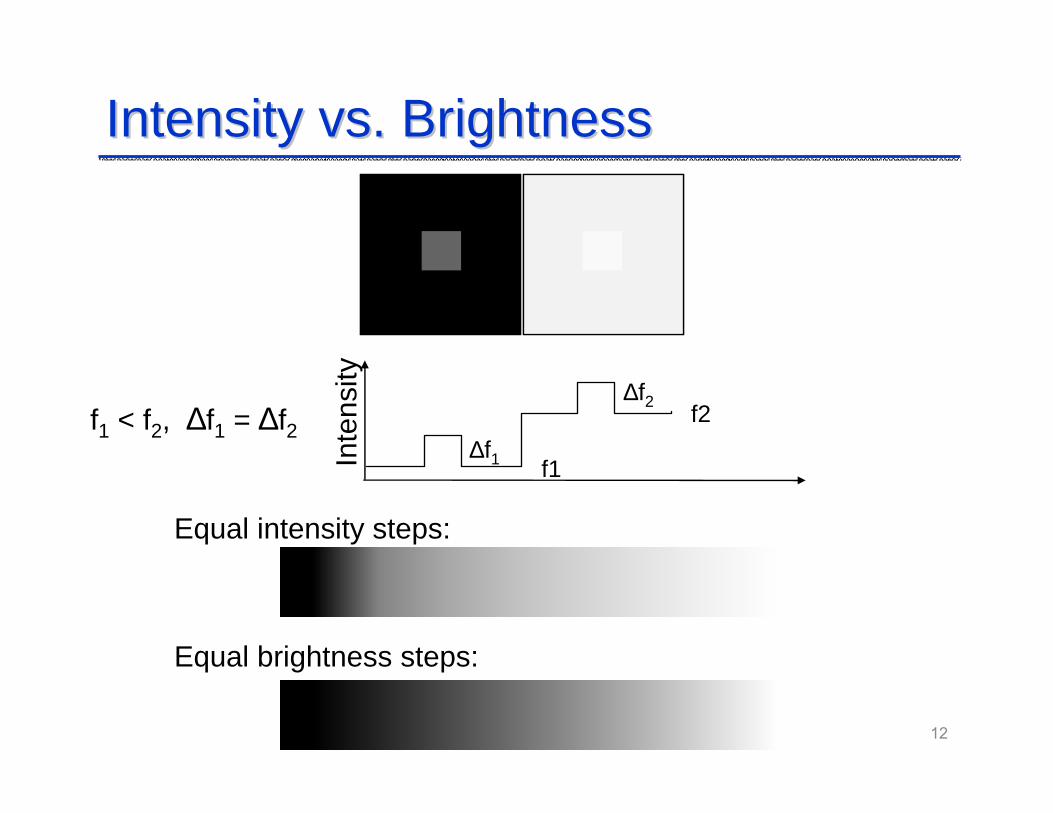
f1 < f2, ∆f1 = ∆f2

Equal intensity steps:

Equal brightness steps:

Intensity vs. BrightnessIntensity vs. Brightness

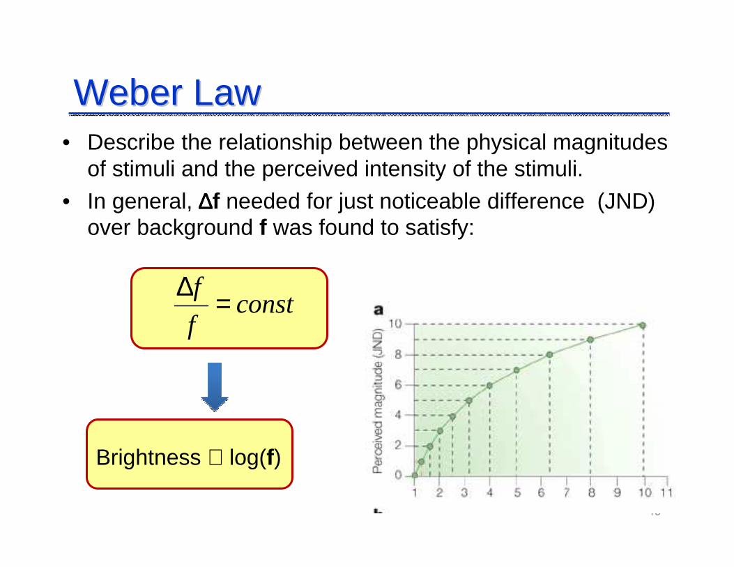
Weber LawWeber Law• Describe the relationship between the physical magnitudes

of stimuli and the perceived intensity of the stimuli.

• In general, ∆∆∆∆f needed for just noticeable difference (JND) over background f was found to satisfy:

13

constf

f =∆

Brightness ∝ log(f)

What about Color Space? What about Color Space?

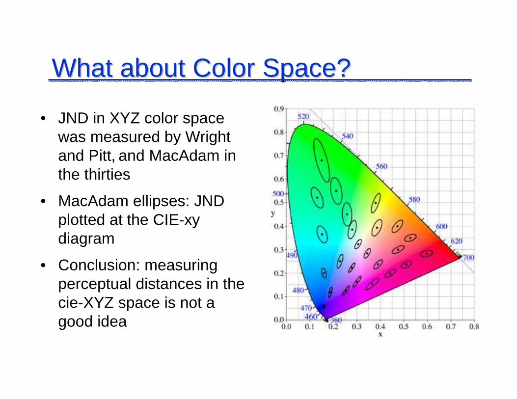
• JND in XYZ color space was measured by Wright and Pitt, and MacAdam in the thirties

• MacAdam ellipses: JND plotted at the CIE-xydiagram

• Conclusion: measuring perceptual distances in the cie-XYZ space is not a good idea

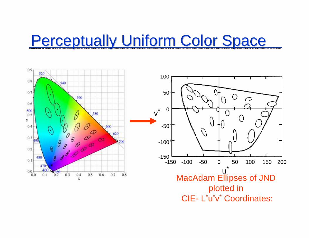
Perceptually Uniform Color SpacePerceptually Uniform Color Space

MacAdam Ellipses of JND plotted in

CIE- L*u*v* Coordinates:

u*-150 -100 -50 0 50 100 150 200

-150

100

50

0

-50

-100

v*

Acquisition SystemAcquisition System

16

World Camera Digitizer DigitalImage

CMOS sensor

100 100 100 100 100

100 0 0 0 100

100 0 0 0 100

100 0 0 0 100

100 100 100 100 100

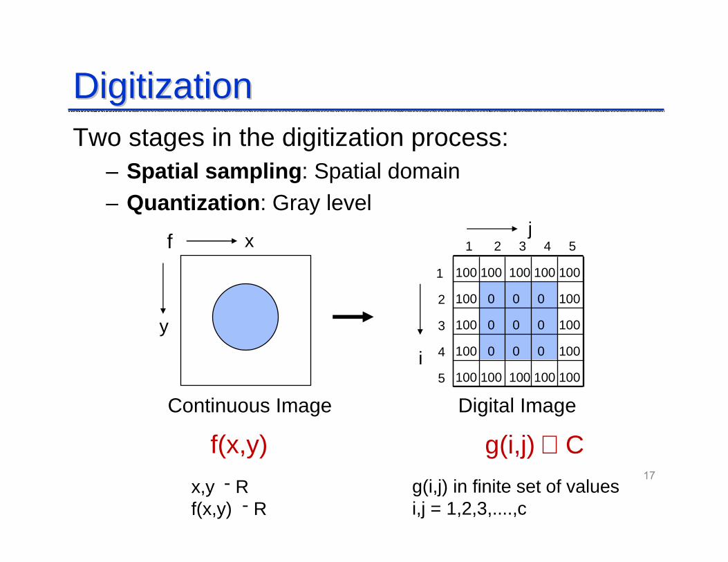
DigitizationDigitizationTwo stages in the digitization process:

– Spatial sampling: Spatial domain– Quantization: Gray level

17

f x

y

1 2 3 4 5

1

2

3

4

5

f(x,y)

Continuous Image Digital Image

g(i,j) ∈ C

j

i

x,y ־ Rf(x,y) ־ R

g(i,j) in finite set of valuesi,j = 1,2,3,....,c

Spatial SamplingSpatial Sampling

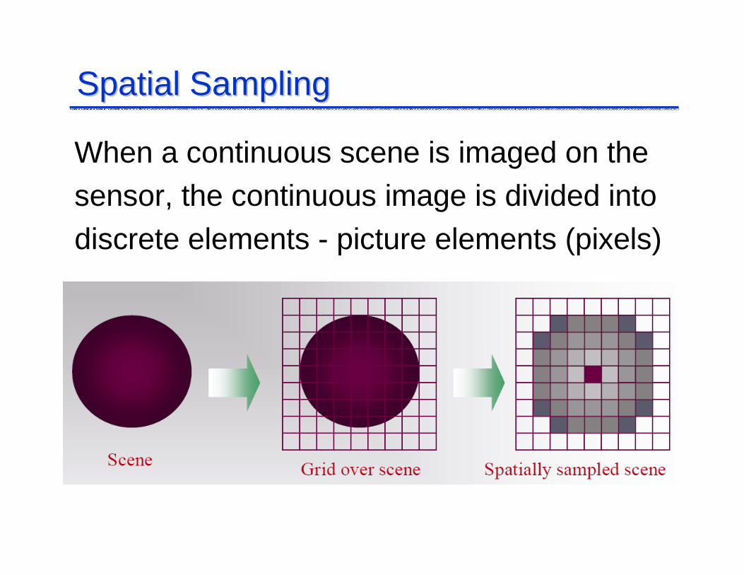
When a continuous scene is imaged on thesensor, the continuous image is divided intodiscrete elements - picture elements (pixels)

Spatial SamplingSpatial Sampling

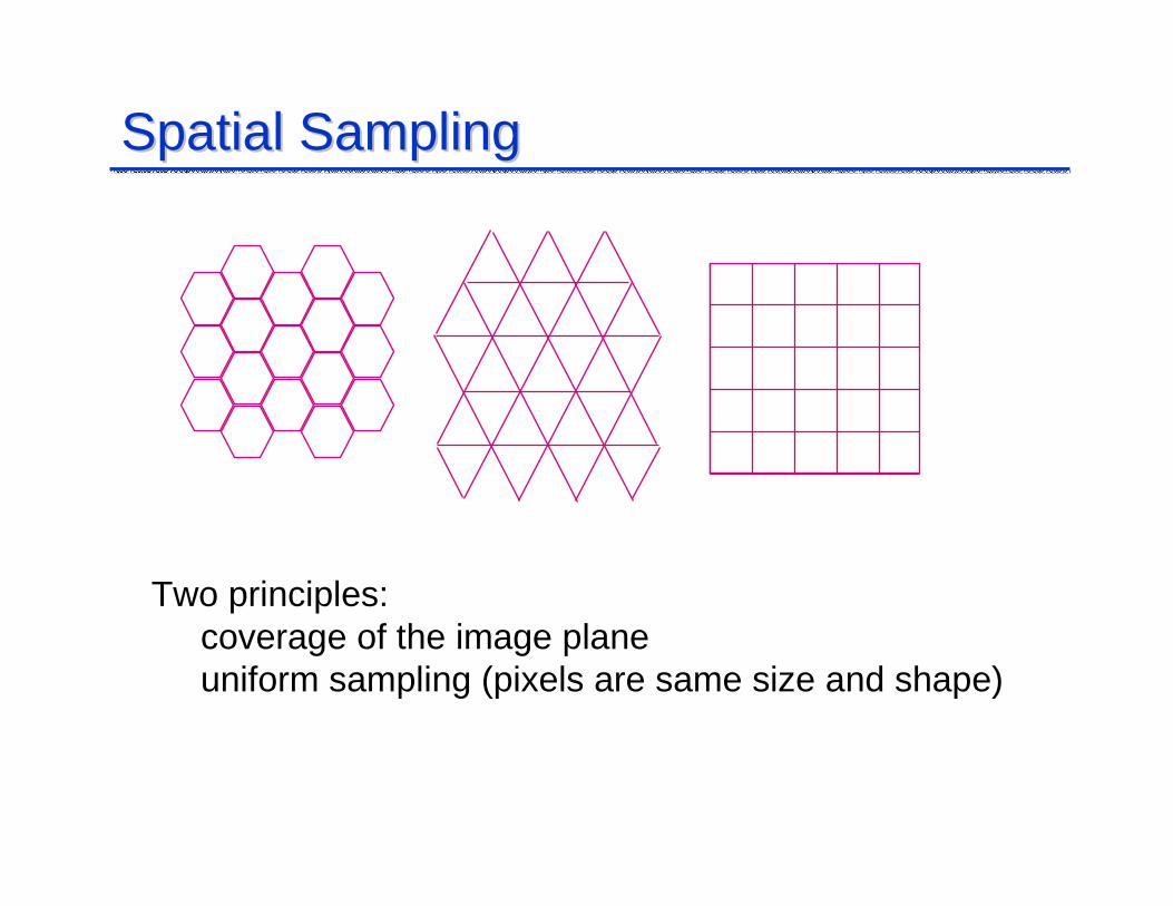
Two principles:coverage of the image planeuniform sampling (pixels are same size and shape)

Spatial Sampling Spatial Sampling

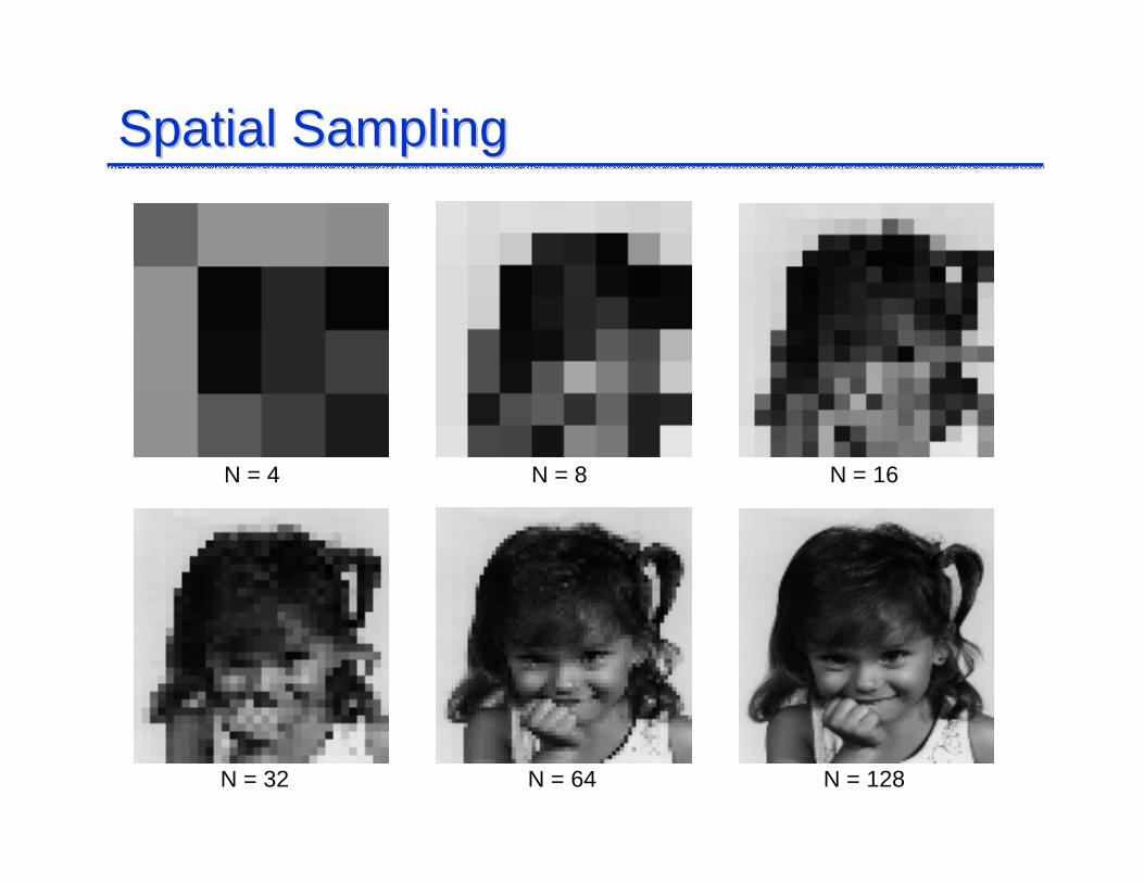
N = 128N = 64N = 32

N = 16N = 8N = 4

0x

Sampling Sampling -- Image ResolutionImage Resolution

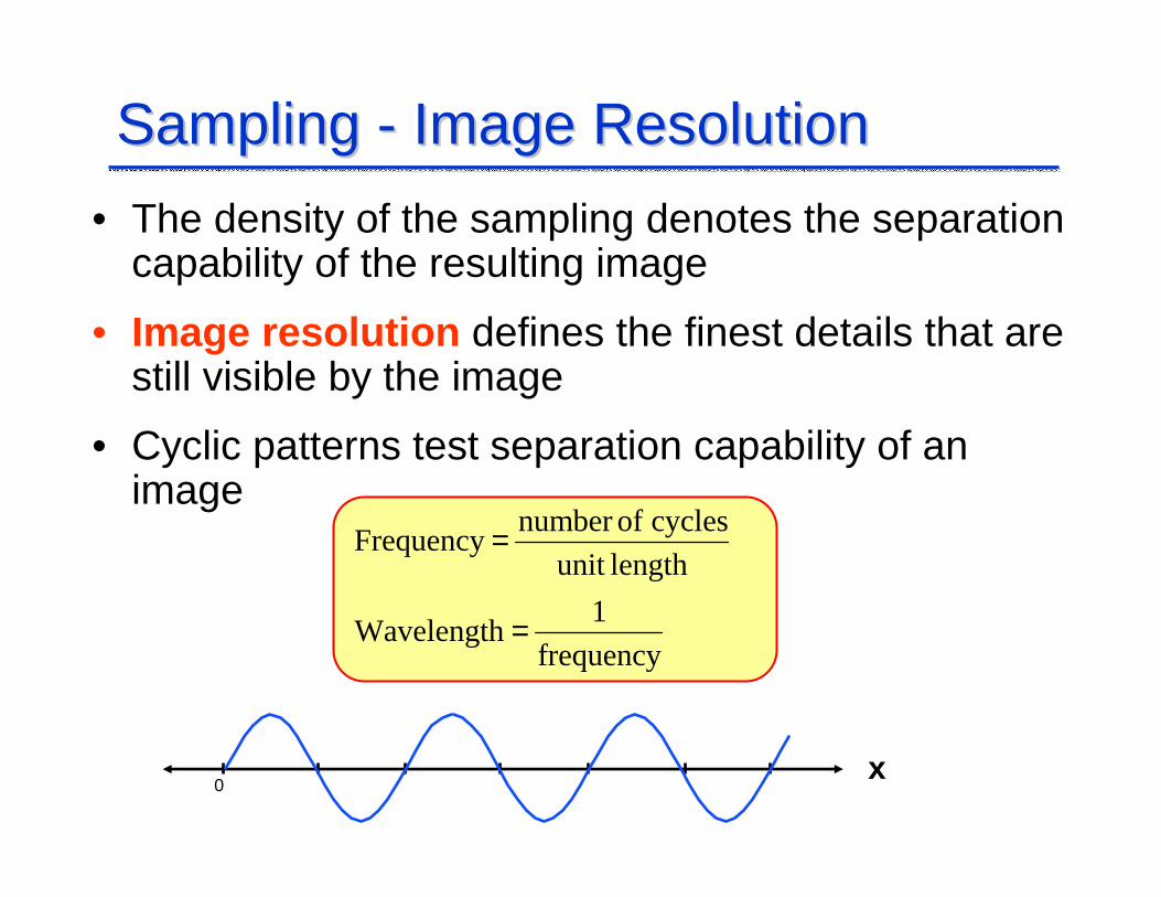
• The density of the sampling denotes the separation capability of the resulting image

• Image resolution defines the finest details that are still visible by the image

• Cyclic patterns test separation capability of an image

frequency

1Wavelength

lengthunit

cyclesofnumberFrequency

=

=

Sampling RateSampling Rate

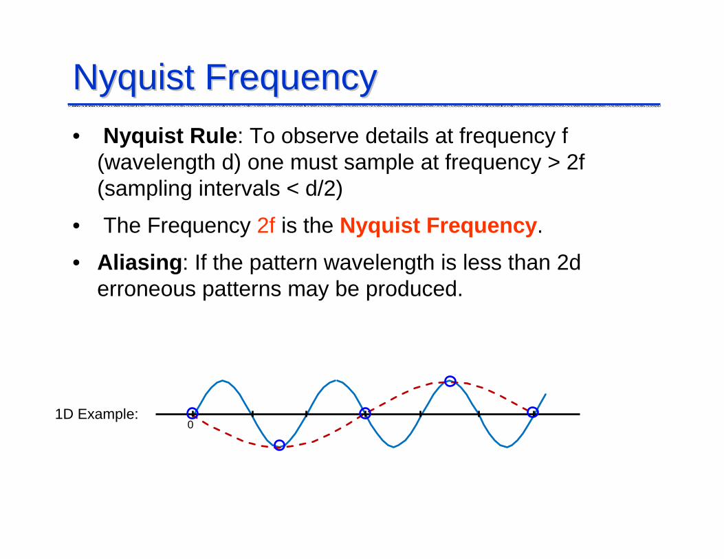
1D Example:0

NyquistNyquist FrequencyFrequency

• Nyquist Rule: To observe details at frequency f (wavelength d) one must sample at frequency > 2f (sampling intervals < d/2)

• The Frequency 2f is the Nyquist Frequency.

• Aliasing: If the pattern wavelength is less than 2d erroneous patterns may be produced.

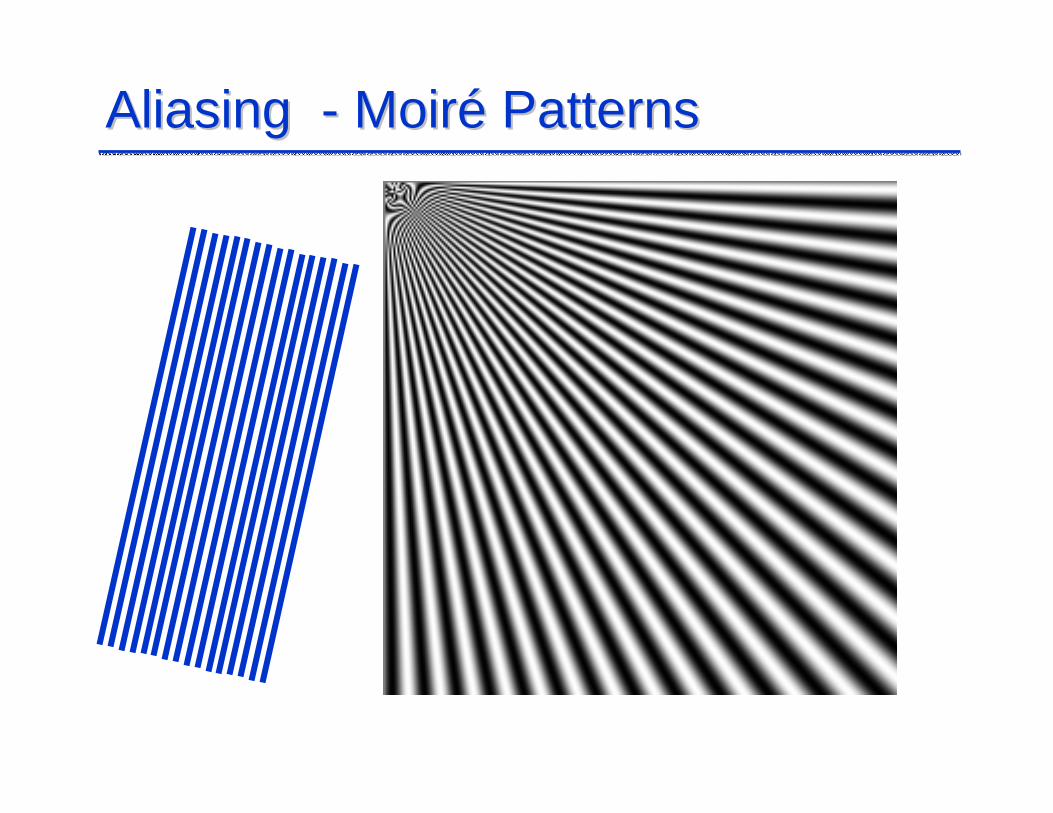
Aliasing Aliasing -- MoirMoiréé PatternsPatterns

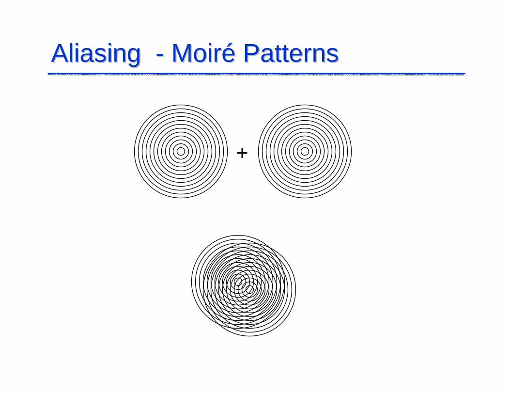
Aliasing Aliasing -- MoirMoiréé PatternsPatterns

+

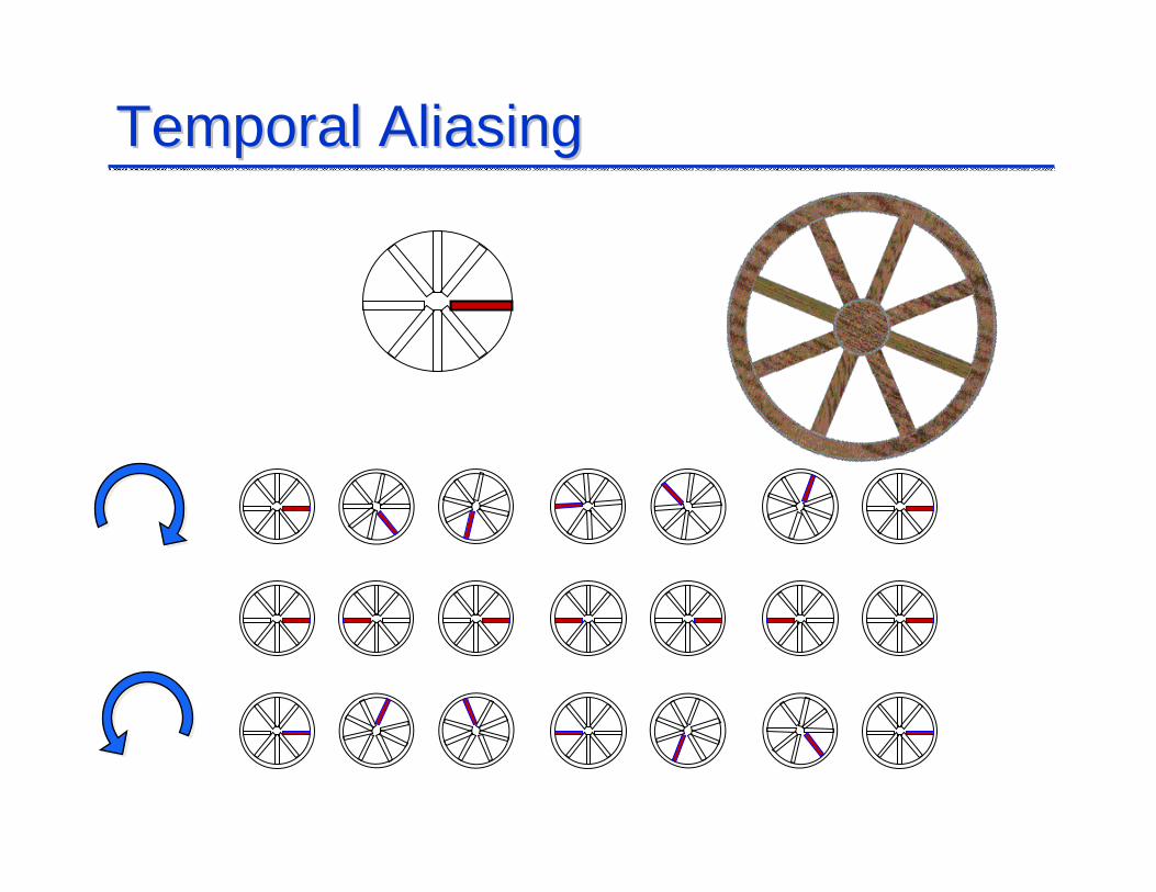
Temporal AliasingTemporal Aliasing

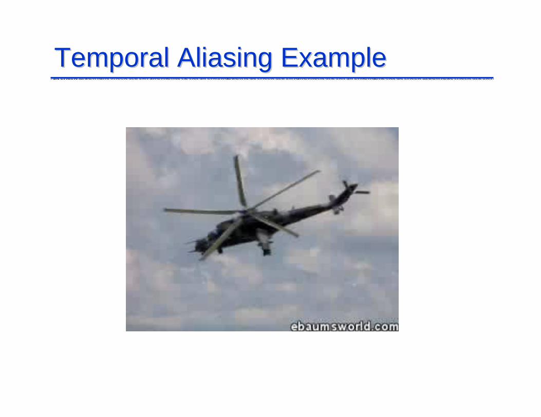
Temporal Aliasing ExampleTemporal Aliasing Example

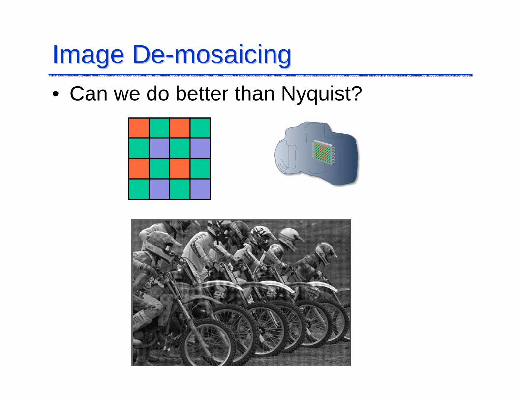
Image DeImage De--mosaicingmosaicing• Can we do better than Nyquist?

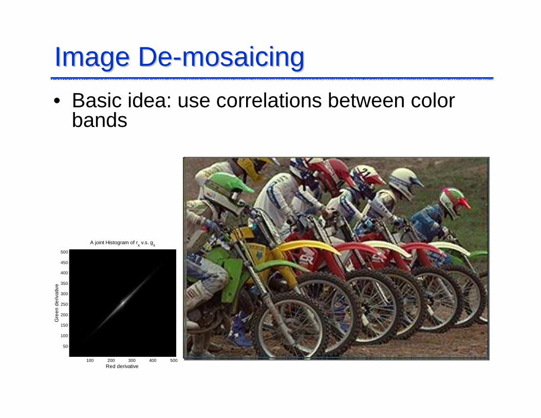
A joint Histogram of rx v.s. g

x

Red derivative

Gre

en d

eriv

ativ

e

100 200 300 400 500

50

100

150

200

250

300

350

400

450

500

Image DeImage De--mosaicingmosaicing

• Basic idea: use correlations between color bands

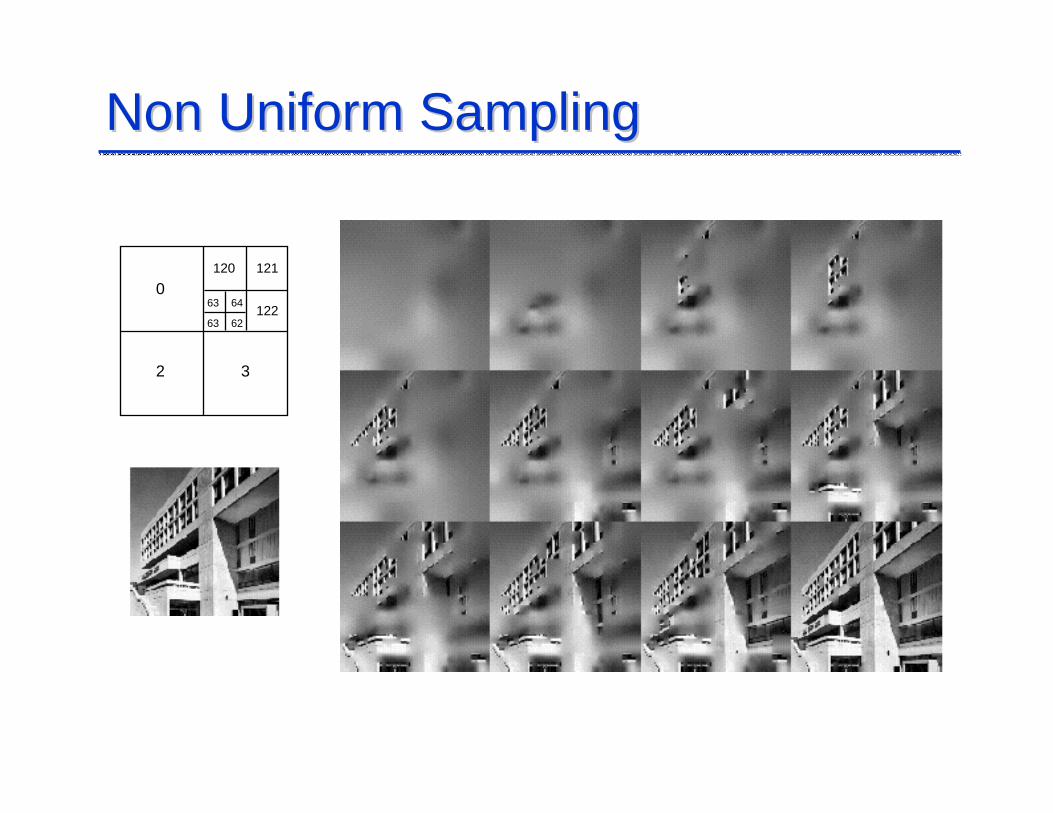
Non Uniform SamplingNon Uniform Sampling

063 64

63 62

2 3

120 121

122

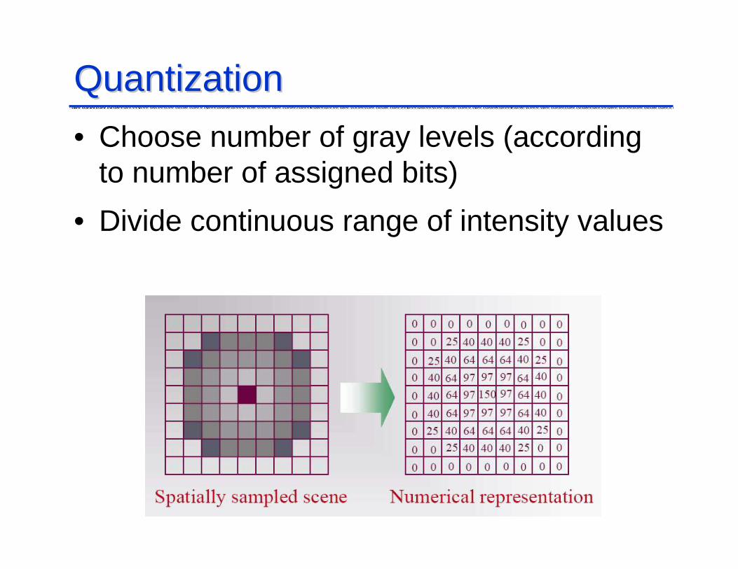
QuantizationQuantization

• Choose number of gray levels (according to number of assigned bits)

• Divide continuous range of intensity values

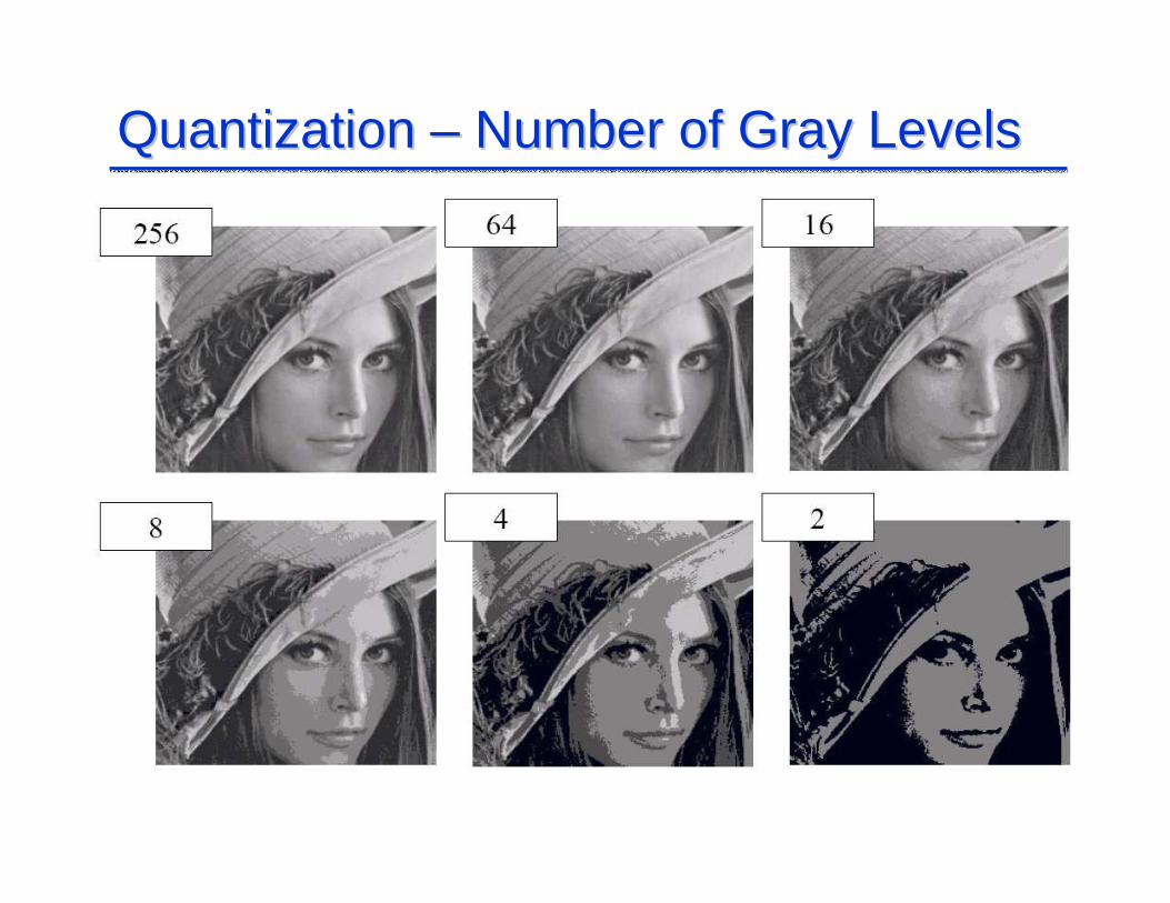
Quantization Quantization –– Number of Gray LevelsNumber of Gray Levels

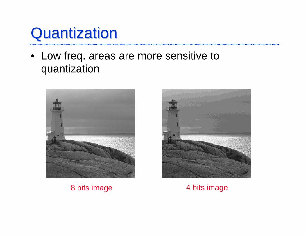
QuantizationQuantization

8 bits image 4 bits image

• Low freq. areas are more sensitive to quantization

0 10 20 30 40 50 60 70 80 90 1000

2

4

6

8

10

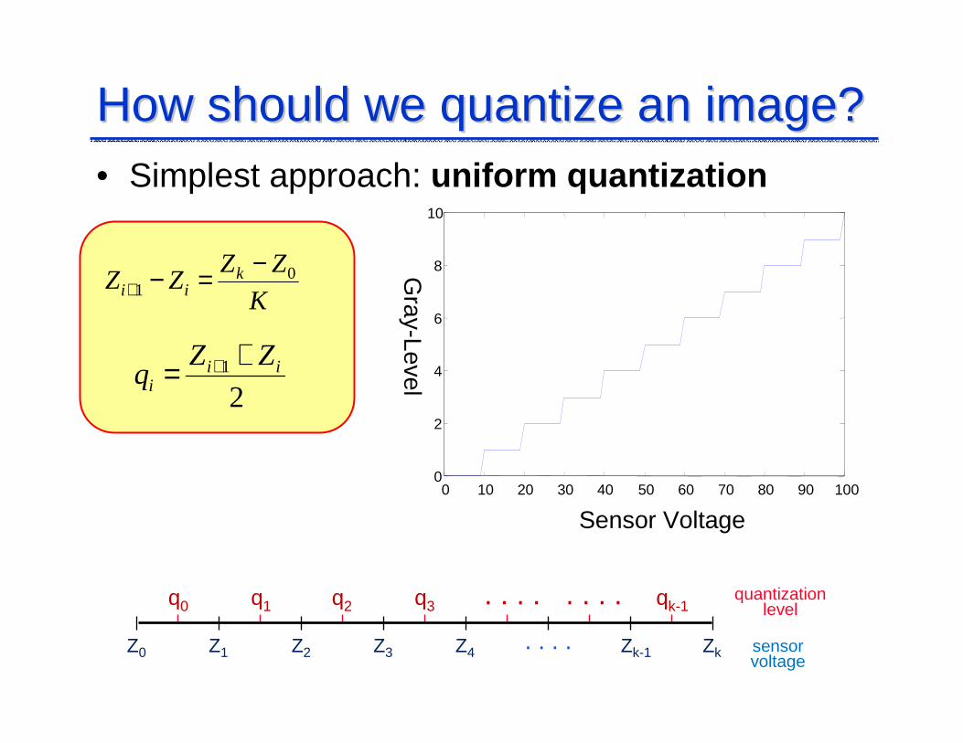
How should we quantize an image? How should we quantize an image? • Simplest approach: uniform quantization

Gray-Level

Sensor Voltage

21 ii

i

ZZq

+= +

K

ZZZZ k

ii0

1

−=−+

Z0 Z1 Z2 Z3 Z4 Zk-1 Zk. . . .

q0 q1 q2 q3 qk-1. . . . . . . .

sensor voltage

quantizationlevel

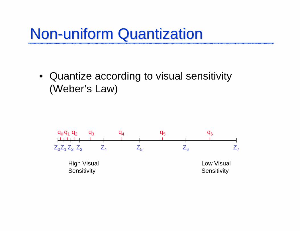
NonNon--uniform Quantizationuniform Quantization

• Quantize according to visual sensitivity (Weber’s Law)

Z7Z6Z5Z4Z3Z1Z0 Z2

q6q5q3q2q0 q4q1

Low Visual Sensitivity

High Visual Sensitivity

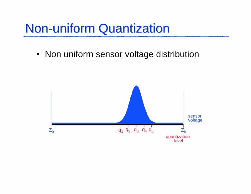
NonNon--uniform Quantizationuniform Quantization

• Non uniform sensor voltage distribution

sensor voltage

quantization level

Z0 Zkq2 q3 q4 q5q1

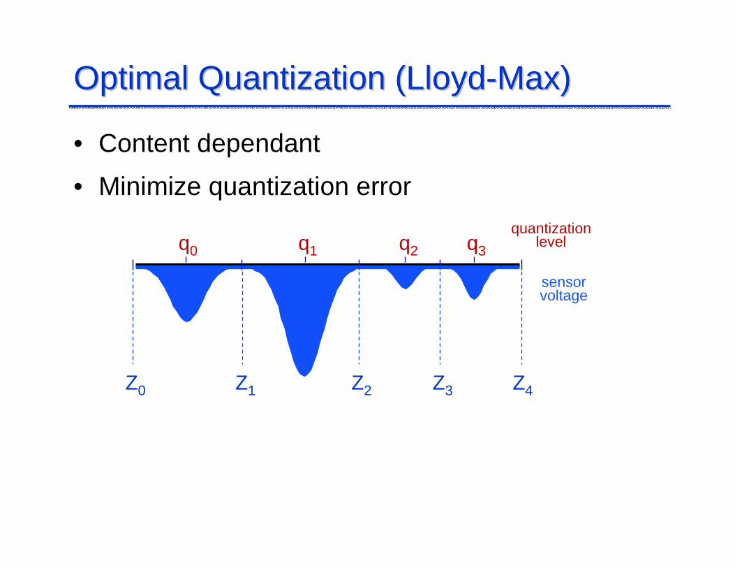
Optimal Quantization (LloydOptimal Quantization (Lloyd--Max)Max)

• Content dependant

• Minimize quantization error

q0 q1 q2 q3

sensor voltage

quantizationlevel

Z0 Z1 Z2 Z3 Z4

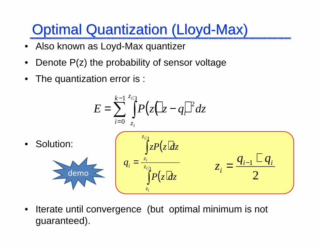
Optimal Quantization (LloydOptimal Quantization (Lloyd--Max)Max)• Also known as Loyd-Max quantizer

• Denote P(z) the probability of sensor voltage

• The quantization error is :

• Solution:

• Iterate until convergence (but optimal minimum is not guaranteed).

( )( ) dzqzzPEk

i

z

z

i

i

i

∑ ∫−

=

+

−=1

0

21

( )

( )∫

∫+

+

=1

1

i

i

i

i

z

z

z

zi

dzzP

dzzzP

q

21 ii

i

qqz

+= −demo

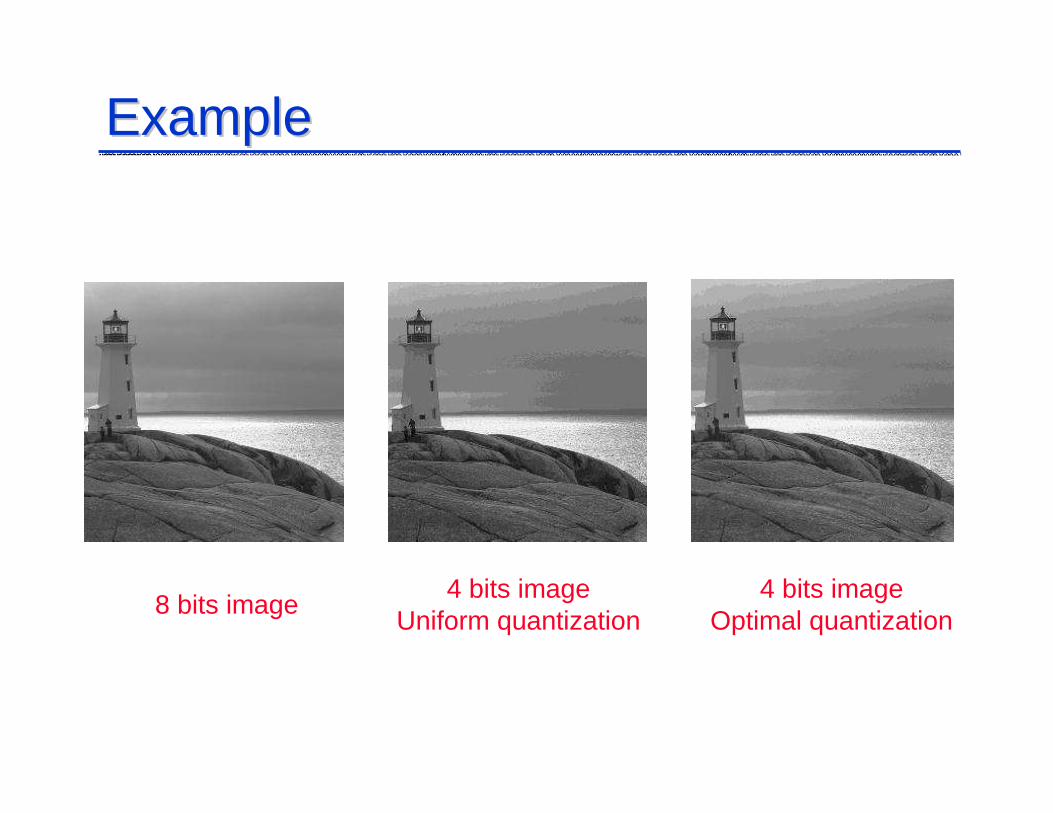
ExampleExample

8 bits image4 bits image

Uniform quantization4 bits image

Optimal quantization

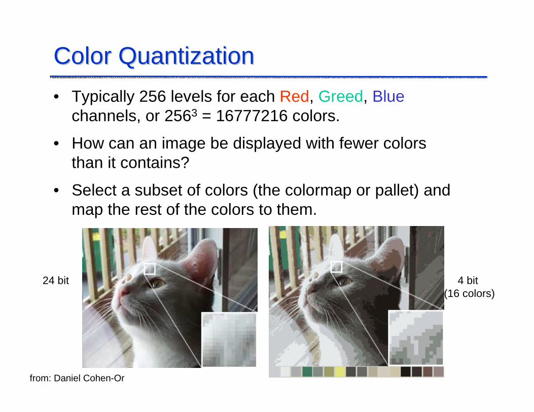
• Typically 256 levels for each Red, Greed, Bluechannels, or 2563 = 16777216 colors.

• How can an image be displayed with fewer colors than it contains?

• Select a subset of colors (the colormap or pallet) and map the rest of the colors to them.

from: Daniel Cohen-Or

Color QuantizationColor Quantization

24 bit 4 bit (16 colors)

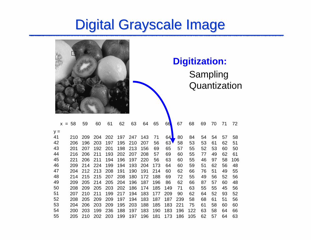
210 209 204 202 197 247 143 71 64 80 84 54 54 57 58 206 196 203 197 195 210 207 56 63 58 53 53 61 62 51 201 207 192 201 198 213 156 69 65 57 55 52 53 60 50 216 206 211 193 202 207 208 57 69 60 55 77 49 62 61 221 206 211 194 196 197 220 56 63 60 55 46 97 58 106 209 214 224 199 194 193 204 173 64 60 59 51 62 56 48 204 212 213 208 191 190 191 214 60 62 66 76 51 49 55 214 215 215 207 208 180 172 188 69 72 55 49 56 52 56 209 205 214 205 204 196 187 196 86 62 66 87 57 60 48 208 209 205 203 202 186 174 185 149 71 63 55 55 45 56 207 210 211 199 217 194 183 177 209 90 62 64 52 93 52 208 205 209 209 197 194 183 187 187 239 58 68 61 51 56 204 206 203 209 195 203 188 185 183 221 75 61 58 60 60 200 203 199 236 188 197 183 190 183 196 122 63 58 64 66 205 210 202 203 199 197 196 181 173 186 105 62 57 64 63

x = 58 59 60 61 62 63 64 65 66 67 68 69 70 71 72

y = 414243444546474849505152535455

Digital Grayscale ImageDigital Grayscale Image

Digitization:SamplingQuantization