II. Example: Simulation of a conjugate heat transfer in a cooling channel of the

furnace for ceramic bricks baking.

1. Problem description

The system ITO Fusch is a

technological line for producing of the

large pieces ceramic bricks. The baking

process in the tunnel furnace is

performed at the one row (large pieces

ceramic bricks) or several row (small

peaces bricks) articles on the wagon,

which pass through tunnel (figure 1). The

bricks are heated in the heating channel.

The backing temperature is kept for a

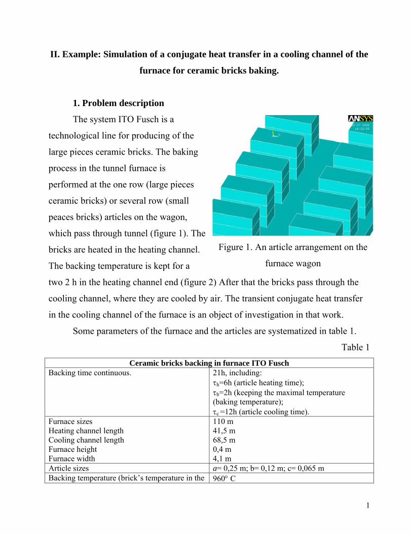
two 2 h in the heating channel end (figure 2) After that the bricks pass through the

cooling channel, where they are cooled by air. The transient conjugate heat transfer

in the cooling channel of the furnace is an object of investigation in that work.

Figure 1. An article arrangement on the

furnace wagon

Some parameters of the furnace and the articles are systematized in table 1.

Table 1 Ceramic bricks backing in furnace ITO Fusch

Backing time continuous. 21h, including: τh=6h (article heating time); τb=2h (keeping the maximal temperature (baking temperature); τc =12h (article cooling time).

Furnace sizes Heating channel length Cooling channel length Furnace height Furnace width

110 m 41,5 m 68,5 m 0,4 m 4,1 m

Article sizes a= 0,25 m; b= 0,12 m; c= 0,065 m Backing temperature (brick’s temperature in the 960° С

1

start of the cooling process) Temperatures of the cooling air of the start and the end of the cooling channel. Temperature-time relation

tinlet=20 °С toutlet=150 °С

τ.0028,0423 −=T Air flow at normal conditions (p=101325Pa and t=0°С)

smVo /12,7 3=&

Air flow velocity at normal conditions Velocity – time variation

Vo=3,5 m/s

τ.00003,048,4.273

0 −== TV

V

Flue gazes

Raw bricks

Air 150 C

Baked bricsk

Air Fuel

Heating channel Cooling channel

Figure 2. Technological scheme of the heating and cooling process

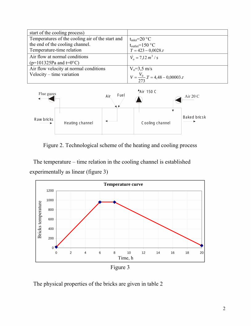
The temperature – time relation in the cooling channel is established

experimentally as linear (figure 3)

Temperature curve

0

200

400

600

800

1000

1200

0 2 4 6 8 10 12 14 16 18 20

Time, h

Bric

ks te

mpe

ratu

re

Figure 3

The physical properties of the bricks are given in table 2

2

Table 2

Conductivity W/(m.K) Specific heat capacity J/(kg.K) Density kg/m3Solid Bricks

0.00051.T0,609

KKK zzyyxx

+=

===

0,264.T765c += 1800ρ =

2. Problem aim: An investigation of the transient heat transfer in the articles in

the cooling channel.

3. Problem solution with ANSYS/FLOTRAN

Figure 4

3.1. Choice of the finite

element type

Preferences > FLOTRAN CFD

Choice of finite element

Fluid 142 for problem solution:

Main Menu /Preprocessor/ Element type/ Add, Edit, Delete/ Add/ FLOTRAN

CFD/ Fluid 142

3.2 Model geometry

3

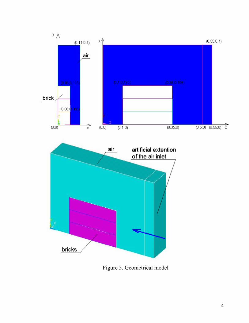
Figure 5. Geometrical model

4

It’s enough to be investigating a half of column of bricks and the air flow,

surrounded it at an assumption of existing of thermal, hydrodynamic and

geometrical symmetries. The wagon movement through the furnace cooling channel

can be modeled with applying a change of the air temperature and velocity on the

model inlet. The air volume must be extended artificially to enable specifying of the

temperature change mode on the air inlet. The geometrical model is made in the

path:

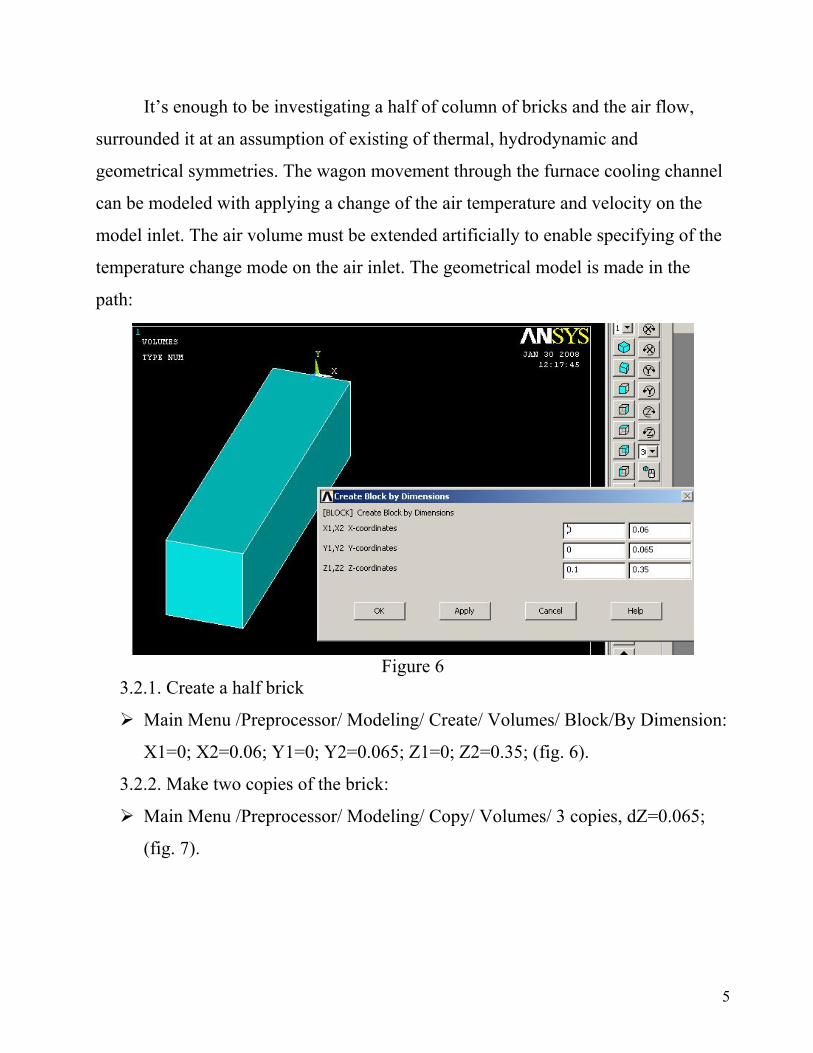
3.2.1. Create a half brick

Figure 6

Main Menu /Preprocessor/ Modeling/ Create/ Volumes/ Block/By Dimension:

X1=0; X2=0.06; Y1=0; Y2=0.065; Z1=0; Z2=0.35; (fig. 6).

3.2.2. Make two copies of the brick:

Main Menu /Preprocessor/ Modeling/ Copy/ Volumes/ 3 copies, dZ=0.065;

(fig. 7).

5

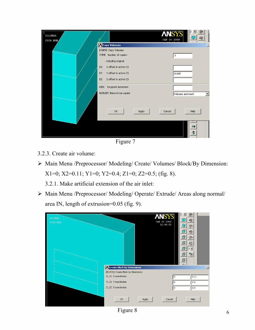
Figure 7

3.2.3. Create air volume:

Main Menu /Preprocessor/ Modeling/ Create/ Volumes/ Block/By Dimension:

X1=0; X2=0.11; Y1=0; Y2=0.4; Z1=0; Z2=0.5; (fig. 8).

3.2.1. Make artificial extension of the air inlet:

Main Menu /Preprocessor/ Modeling/ Operate/ Extrude/ Areas along normal/

area IN, length of extrusion=0.05 (fig. 9).

6

Figure 8

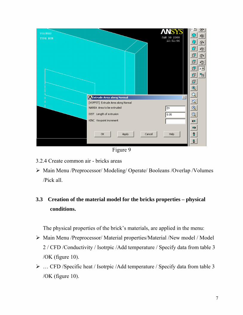
Figure 9

3.2.4 Create common air - bricks areas

Main Menu /Preprocessor/ Modeling/ Operate/ Booleans /Overlap /Volumes

/Pick all.

3.3 Creation of the material model for the bricks properties – physical

conditions.

The physical properties of the brick’s materials, are applied in the menu:

Main Menu /Preprocessor/ Material properties/Material /New model / Model

2 / CFD /Conductivity / Isotrpic /Add temperature / Specify data from table 3

/OK (figure 10).

… CFD /Specific heat / Isotrpic /Add temperature / Specify data from table 3

/OK (figure 10).

7

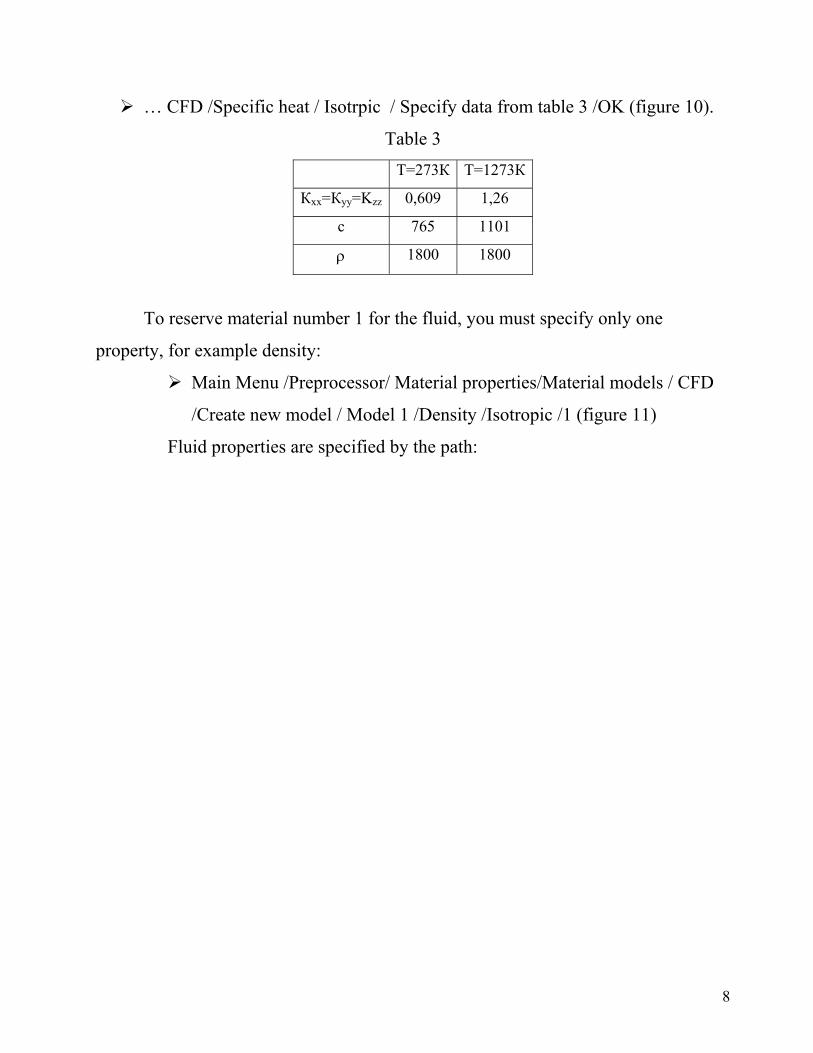
… CFD /Specific heat / Isotrpic / Specify data from table 3 /OK (figure 10).

Table 3 Т=273К Т=1273К

Кхх=Куу=Kzz 0,609 1,26

с 765 1101

ρ 1800 1800

To reserve material number 1 for the fluid, you must specify only one

property, for example density:

Main Menu /Preprocessor/ Material properties/Material models / CFD

/Create new model / Model 1 /Density /Isotropic /1 (figure 11)

Fluid properties are specified by the path:

8

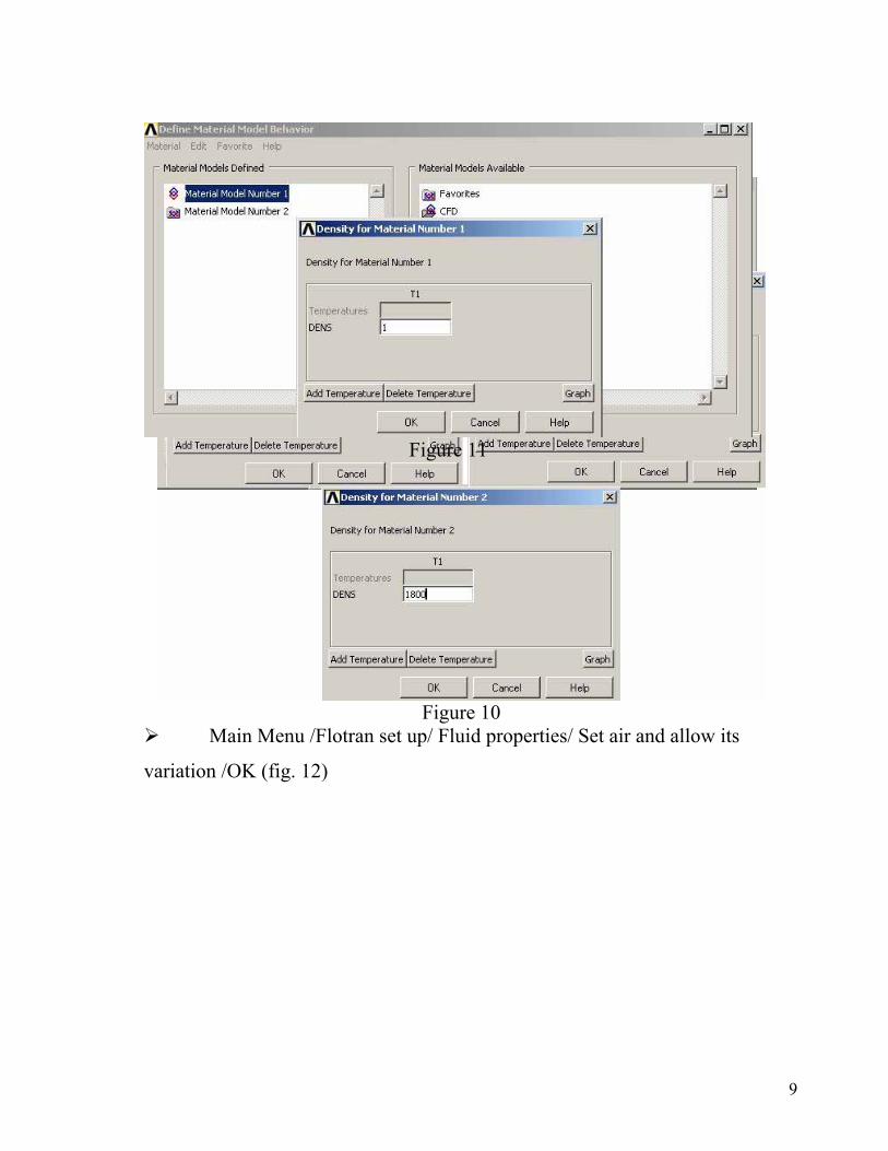
Main Menu /Flotran set up/ Fluid properties/ Set air and allow its

variation /OK (fig. 12)

Figure 10

Figure 11

9

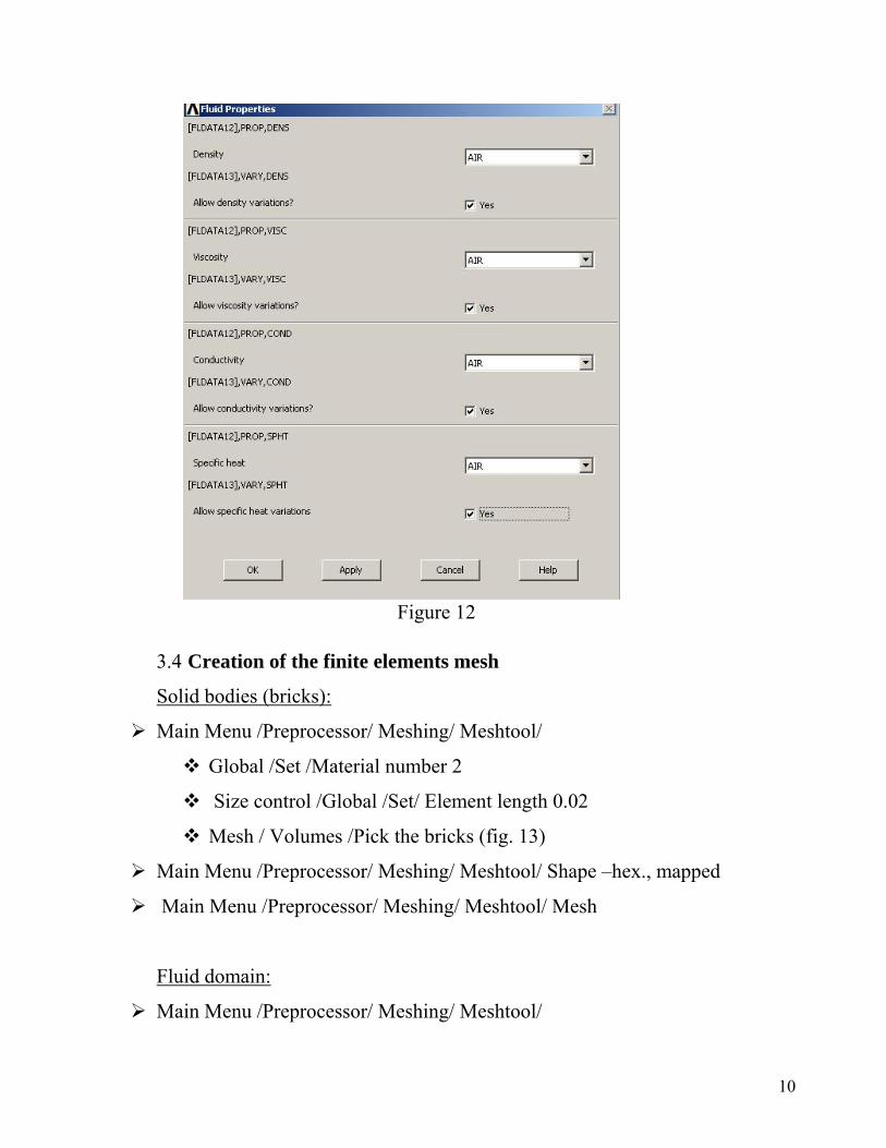
Figure 12

3.4 Creation of the finite elements mesh

Solid bodies (bricks):

Main Menu /Preprocessor/ Mеshing/ Meshtool/

Global /Set /Material number 2

Size control /Global /Set/ Element length 0.02

Mesh / Volumes /Pick the bricks (fig. 13)

Main Menu /Preprocessor/ Mеshing/ Meshtool/ Shape –hex., mapped

Main Menu /Preprocessor/ Mеshing/ Meshtool/ Mesh

Fluid domain:

Main Menu /Preprocessor/ Mеshing/ Meshtool/

10

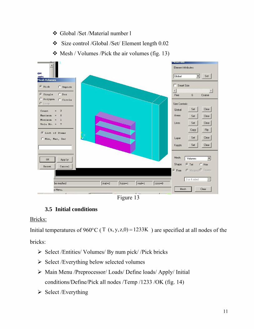
Global /Set /Material number l

Size control /Global /Set/ Element length 0.02

Mesh / Volumes /Pick the air volumes (fig. 13)

Figure 13

3.5 Initial conditions

Bricks:

Initial temperatures of 960°С ( K2331z,0)y,(x,T = ) are specified at all nodes of the

bricks:

Select /Entities/ Volumes/ By num pick/ /Pick bricks

Select /Everything below selected volumes

Main Menu /Preprocessor/ Loads/ Define loads/ Apply/ Initial

conditions/Define/Pick all nodes /Temp /1233 /OK (fig. 14)

Select /Everything

11

Figure 14

Fluid domain:

Initial temperatures of 150°С ( K423z,0)y,(x,T = ) are specified:

Main Menu /Flotran set up/ Flow environment/ Reference conditions

/nominal, stagnation and total temperatures 423/ Reference pressure 101325

/OK (fig. 15)

Figure 15

12

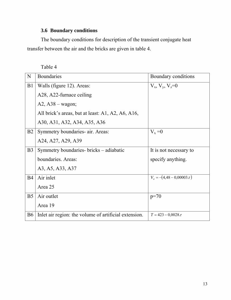
3.6 Boundary conditions

The boundary conditions for description of the transient conjugate heat

transfer between the air and the bricks are given in table 4.

Table 4

N Boundaries Boundary conditions

B1 Walls (figure 12). Areas:

A28, A22-furnace ceiling

A2, A38 – wagon;

All brick’s areas, but at least: A1, A2, A6, A16,

A30, A31, A32, A34, A35, A36

Vx, Vy, Vz=0

B2 Symmetry boundaries- air. Areas:

A24, A27, A29, A39

Vx =0

B3 Symmetry boundaries- bricks – adiabatic

boundaries. Areas:

A3, A5, A33, A37

It is not necessary to

specify anything.

B4 Air inlet

Area 25

( )τ.00003,048,4 −−=zV

B5 Air outlet

Area 19

p=70

B6 Inlet air region: the volume of artificial extension. τ.0028,0423 −=T

13

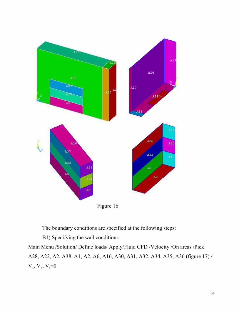
Figure 16

The boundary conditions are specified at the following steps:

B1) Specifying the wall conditions.

Main Menu /Solution/ Define loads/ Apply/Fluid CFD /Velocity /On areas /Pick

A28, A22, A2, A38, A1, A2, A6, A16, A30, A31, A32, A34, A35, A36 (figure 17) /

Vx, Vy, Vz=0

14

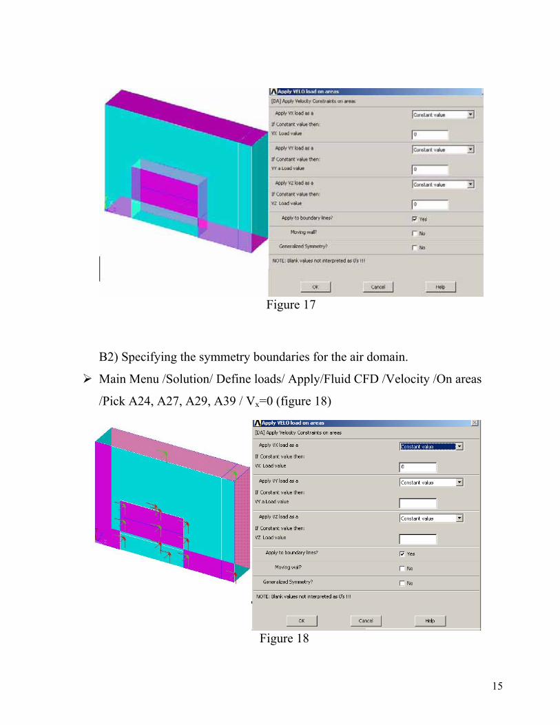
Figure 17

B2) Specifying the symmetry boundaries for the air domain.

Main Menu /Solution/ Define loads/ Apply/Fluid CFD /Velocity /On areas

/Pick A24, A27, A29, A39 / Vx=0 (figure 18)

Figure 18

15

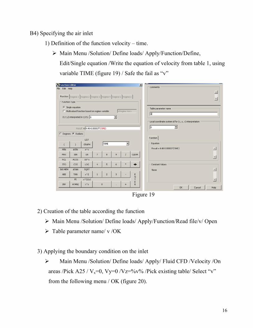
B4) Specifying the air inlet

1) Definition of the function velocity – time.

Main Menu /Solution/ Define loads/ Apply/Function/Define,

Edit/Single equation /Write the equation of velocity from table 1, using

variable TIME (figure 19) / Safe the fail as “v”

Figure 19

2) Creation of the table according the function

Main Menu /Solution/ Define loads/ Apply/Function/Read file/v/ Open

Table parameter name/ v /OK

3) Applying the boundary condition on the inlet

Main Menu /Solution/ Define loads/ Apply/ Fluid CFD /Velocity /On

areas /Pick A25 / Vx=0, Vy=0 /Vz=%v% /Pick existing table/ Select “v”

from the following menu / OK (figure 20).

16

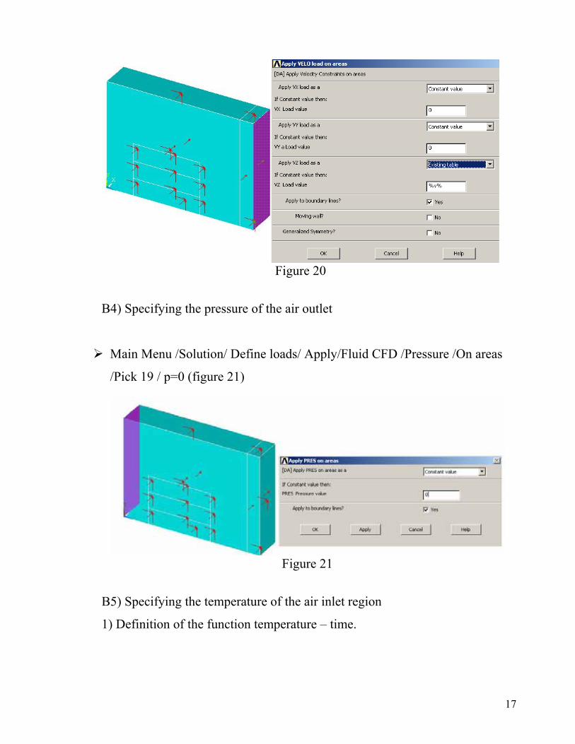
Figure 20

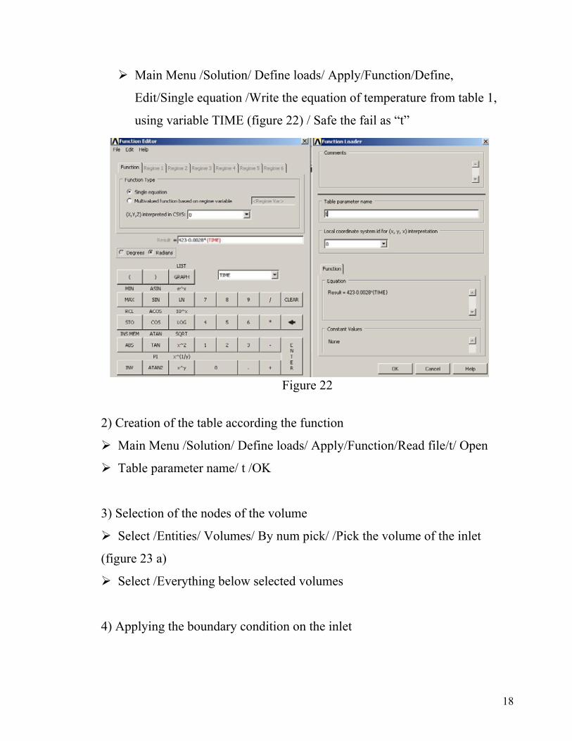
B4) Specifying the pressure of the air outlet

Main Menu /Solution/ Define loads/ Apply/Fluid CFD /Pressure /On areas

/Pick 19 / p=0 (figure 21)

B5) Specifying the temperature of the air inlet region

1) Definition of the function temperature – time.

Figure 21

17

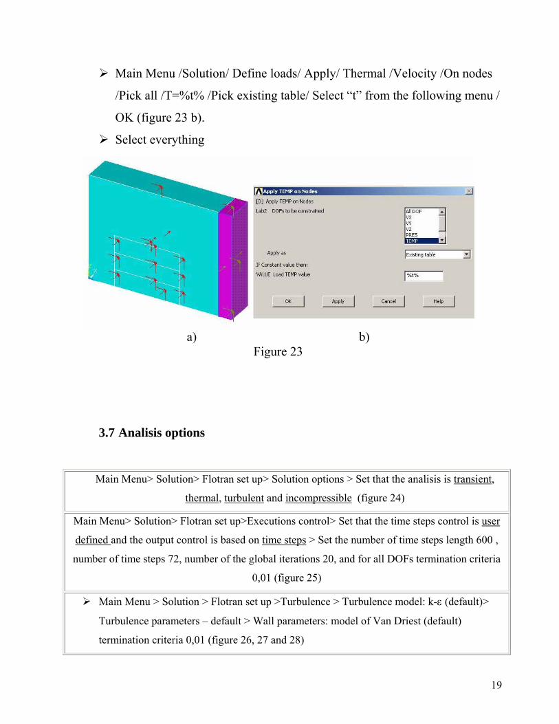
Main Menu /Solution/ Define loads/ Apply/Function/Define,

Edit/Single equation /Write the equation of temperature from table 1,

using variable TIME (figure 22) / Safe the fail as “t”

Figure 22

2) Creation of the table according the function

Main Menu /Solution/ Define loads/ Apply/Function/Read file/t/ Open

Table parameter name/ t /OK

3) Selection of the nodes of the volume

Select /Entities/ Volumes/ By num pick/ /Pick the volume of the inlet

(figure 23 a)

Select /Everything below selected volumes

4) Applying the boundary condition on the inlet

18

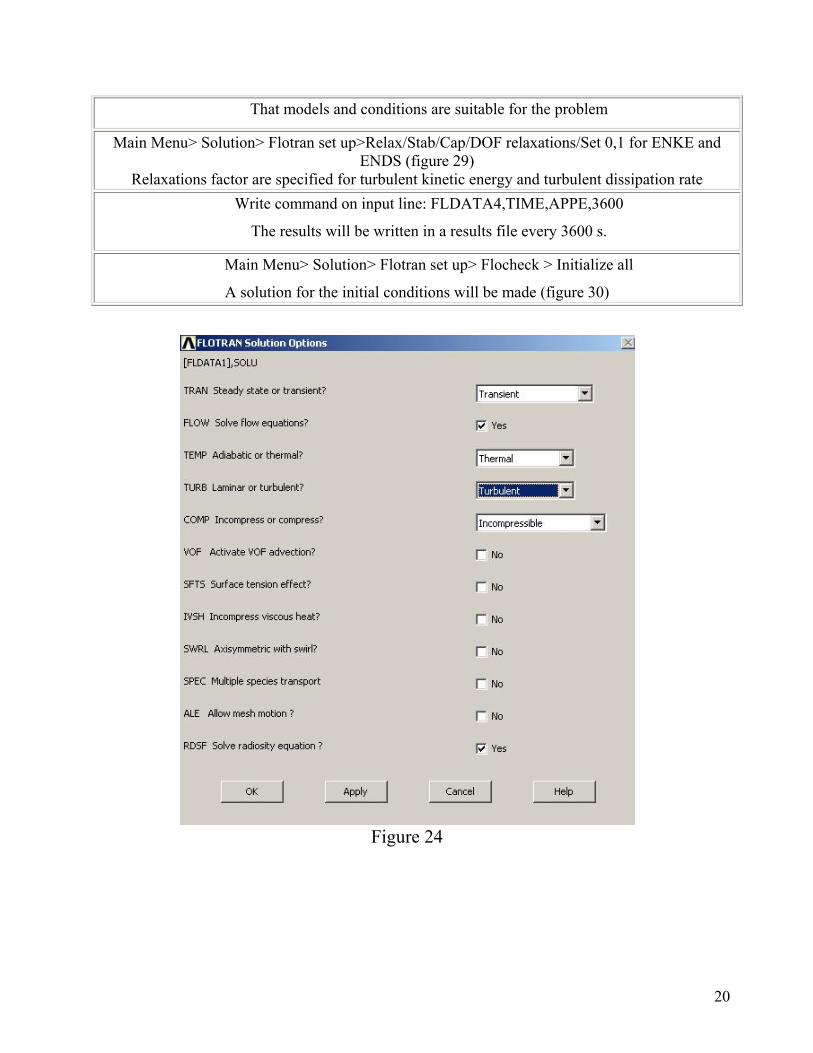
Main Menu /Solution/ Define loads/ Apply/ Thermal /Velocity /On nodes

/Pick all /T=%t% /Pick existing table/ Select “t” from the following menu /

OK (figure 23 b).

Select everything

a) b)

Figure 23

3.7 Analisis options

Main Menu> Solution> Flotran set up> Solution options > Set that the analisis is transient,

thermal, turbulent and incompressible (figure 24)

Main Menu> Solution> Flotran set up>Executions control> Set that the time steps control is user

defined and the output control is based on time steps > Set the number of time steps length 600 ,

number of time steps 72, number of the global iterations 20, and for all DOFs termination criteria

0,01 (figure 25)

Main Menu > Solution > Flotran set up >Turbulence > Turbulence model: k-ε (default)>

Turbulence parameters – default > Wall parameters: model of Van Driest (default)

termination criteria 0,01 (figure 26, 27 and 28)

19

That models and conditions are suitable for the problem

Main Menu> Solution> Flotran set up>Relax/Stab/Cap/DOF relaxations/Set 0,1 for ENKE and ENDS (figure 29)

Relaxations factor are specified for turbulent kinetic energy and turbulent dissipation rate Write command on input line: FLDATA4,TIME,APPE,3600

The results will be written in a results file every 3600 s.

Main Menu> Solution> Flotran set up> Flocheck > Initialize all

A solution for the initial conditions will be made (figure 30)

Figure 24

20

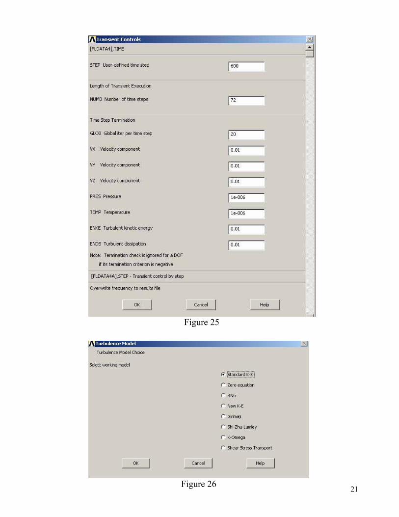
Figure 25

21

Figure 26

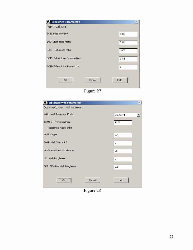
Figure 27

Figure 28

22

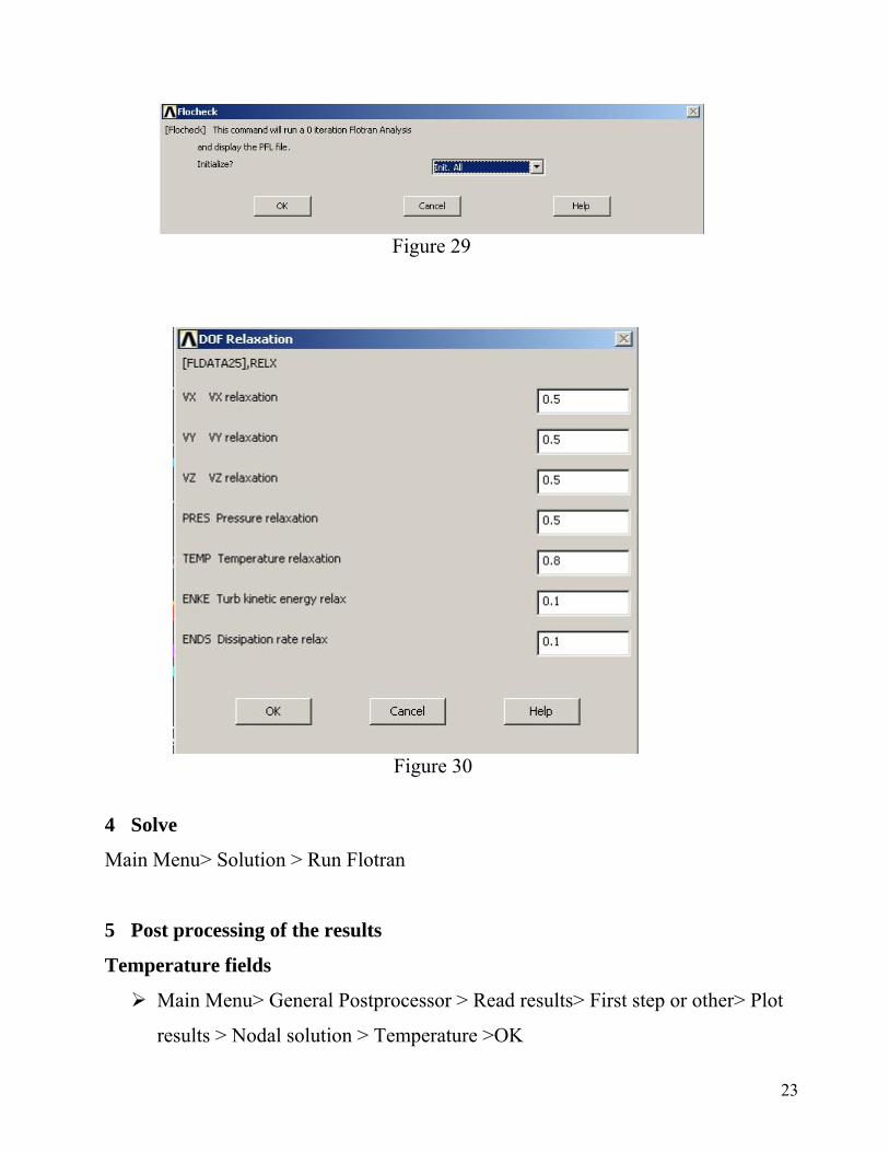
Figure 29

Figure 30

4 Solve

Main Menu> Solution > Run Flotran

5 Post processing of the results

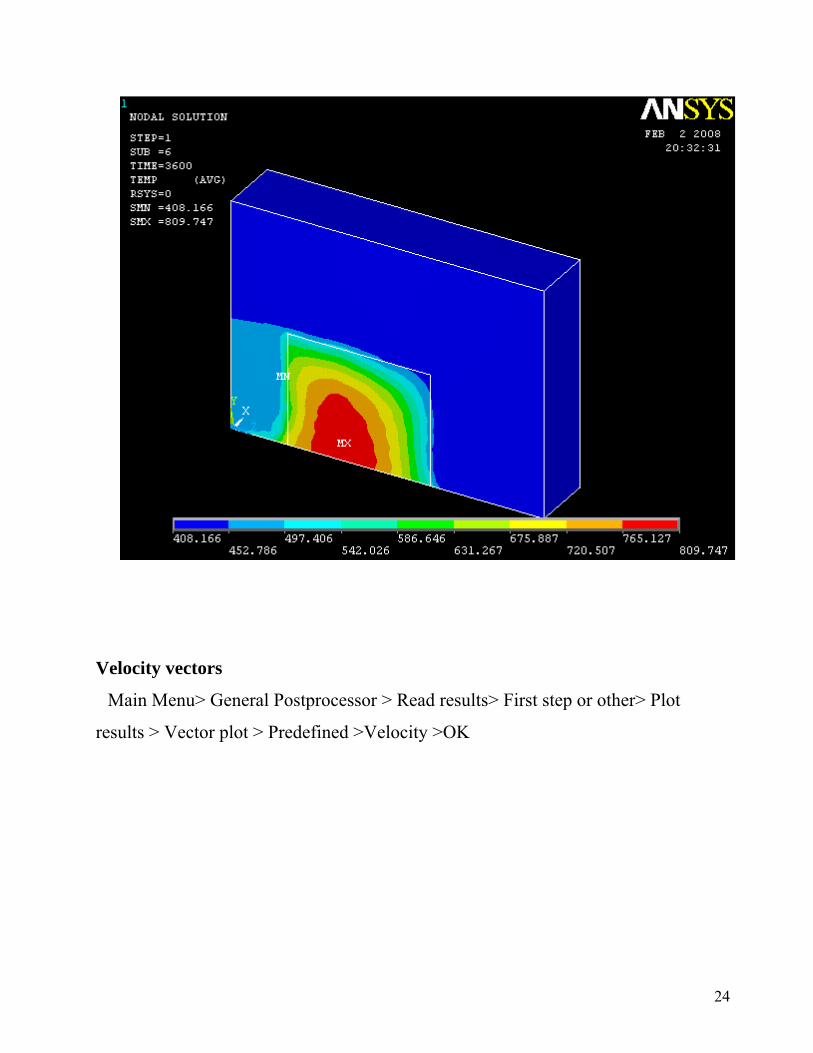
Temperature fields

Main Menu> General Postprocessor > Read results> First step or other> Plot

results > Nodal solution > Temperature >OK

23

Velocity vectors

Main Menu> General Postprocessor > Read results> First step or other> Plot

results > Vector plot > Predefined >Velocity >OK

24

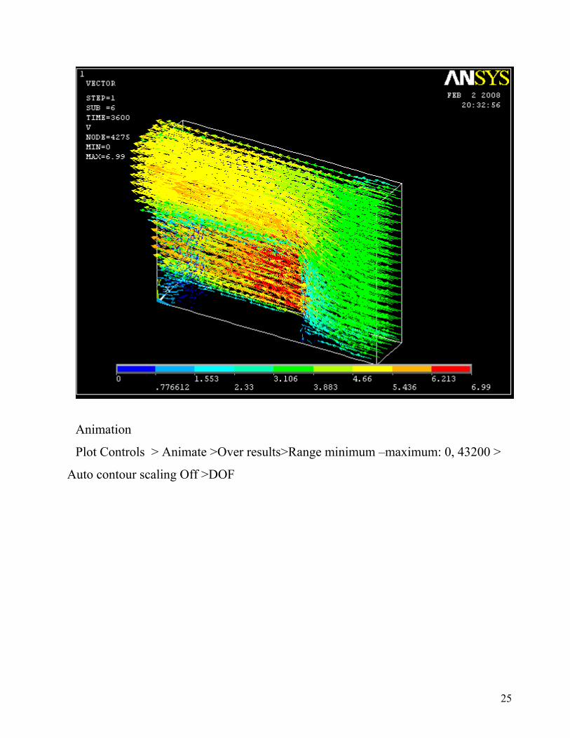
Animation

Plot Controls > Animate >Over results>Range minimum –maximum: 0, 43200 >

Auto contour scaling Off >DOF

25