2nd Colloque INCA23-24 Octobre 2008

Conjugate Heat Transfer with Large Eddy Simulation.Application to Gas Turbine Components.

F. Duchaine1, S. Mendez1, F. Nicoud2, A. Corpron3, V. Moureau3 and T. Poinsot1,4

Conjugate heat transfer is a key issue in combustion: the interaction of reacting flows andhot gases with colder walls is actually a main design constraint in gas turbines. For example,multiperforated plates commonly used in combustion chambers to cool walls must be able tosustain the high fluxes produced in the chamber. After combustion, the interaction of the hotburnt gases with the high pressure stator and the first turbine blades conditions the temperatureand pressure levels reached in the combustor, and thereforethe engine efficiency.Conjugate heat transfer is a difficult field and most existingtools are developped for chained(rather than coupled), steady (rather than transient) phenomena: the fluid flow is computedusing a RANS (Reynolds Averaged Navier-Stokes) solver. During this work, a fully parallelenvironnement for conjugate heat transfer has been developed and applied to two configurationsof interest for the design of combustion devices. The numerical tool is based on a reactive LES(Large Eddy Simulations) code and a solid conduction solverthat can exchange data via asupervisor.An unsteady wall/flame interaction is used to assess the the precision and the order of the cou-pled solutions depending on the coupling frequency. It is shown that the temperature and theflux across the wall are well reproduced when the codes are coupled with a time scale of theorder of the smallest time scale. An experimental film-cooled turbine vane is studied in order toreach a steady state. The solutions from the conjugate analyses and an adiabatic wall convec-tion are compared to experimental results. Concerning pressure profiles, both simulations showa good agreement with experimental results. Due to thermal conduction in the blade, conju-gate results has a lower mean intrado temperature than adiabatic simulation and reproduce theexperimental cooling efficiency quite well.

INTRODUCTION

Conjugate heat transfer is a key issue in combustion [1, 2]: the interaction of hot gases and reacting flowswith colder walls is a key phenomenon in all chambers and is actually a main design constraint in gasturbines. For example, multi-perforated plates are commonly used in gas turbines combustion chambers tocool walls and they must be able to sustain the high fluxes produced in the chamber. After combustion, theinteraction of the hot burnt gases with the high pressure stator and the first turbine blades conditions thetemperature and pressure levels reached in the combustor, and therefore the engine efficiency.Conjugate heat transfer is a difficult field and most existingtools are developed for chained (rather thancoupled), steady (rather than transient) phenomena: the fluid flow is brought to convergence using a RANS(Reynolds Averaged Navier-Stokes) solver for a given set ofskin temperatures [3, 4, 5]. The heat fluxespredicted by the RANS solver are then transferred to a heat transfer solver which produces a new set ofskin temperatures. A few iterations are generally sufficient to reach convergence. There are circumstanceshowever where this chaining method must be replaced by a fullcoupling approach. Flames interacting withwalls for example, may require a simultaneous resolution ofthe temperature within the solid and aroundit. More generally, the introduction of LES to replace RANS leads to full coupling since LES provides theunsteady evolution of all flow variables.Fully coupled conjugate heat transfer requires to take intoaccount multiple questions. Among them, twoissues were considered for the present work:

• The time scales of the flow and of the solid are generally very different. In a gas turbine, a bladesubmitted to the flow exiting from a combustion chamber has a thermal characteristic time scale ofthe order of a few seconds while the flow-through time along the blade is less than1 ms. As aconsequence, the frequency of the exchanges between the codes is critical for the precision, stabilityand restitution time of the computations.

1CERFACS, CFD team, 42 Av Coriolis, 31057 Toulouse, France2Un. Montpellier II3TURBOMECA, Bordes, France4IMF Toulouse, INP de Toulouse and CNRS, 31400 Toulouse , France

• Coupling the two phenomena must be performed on massively parallel machines where the codesmust be not only coupled but synchronized to exploit the power of the machines.

During this work, these two issues have been studied using two examples of conjugate heat transfer: aflame interacting with a wall in section II and a blade submitted to a flow of hot gases in section III. Bothproblems have considerable impact on the design of combustion devices. Section I deals with the codesused to this studies as well as the coupling strategies.

I SOLVERS AND COUPLING STRATEGIES

The AVBP code is used for the fluid [6, 7]. It solves the compressible reacting Navier-Stokes equationswith a third-order scheme for spatial differencing and a Runge Kutta time advancement [8, 9]. Boundaryconditions are handled with the NSCBC formulation [10, 9].For the resolution of the heat transfer equation within solids, a simplified version of AVBP, called AVTP,was developed. It uses the same data structure as AVBP. It is coupled to AVBP using a software calledPALM [11]. For all present examples, the skin meshes are the same for the fluid and the solid so that nointerpolation error is introduced at this level.The coupling strategy between AVBP and AVTP depends on the objectives of the simulation and is charac-terized by two issues:

• Synchronization in physical time: the physical time computed by the two codes between two infor-mation exchanges may be the same or not.5 We will impose that between two coupling events, theflow is advanced in time of a quantityαfτf whereτf is a flow characteristic time. Simultaneously,the solid is advanced of a timeαsτs whereτs is a characteristic time for heat propagation throughthe solid. Two limit cases are of interest: (1)αs = αf ensures that both solid and fluid converge tosteady state at the same rate (the two domains are then not synchronized in physical time) and (2)αfτf = αsτs ensures that the two solvers are synchronized in physical time.

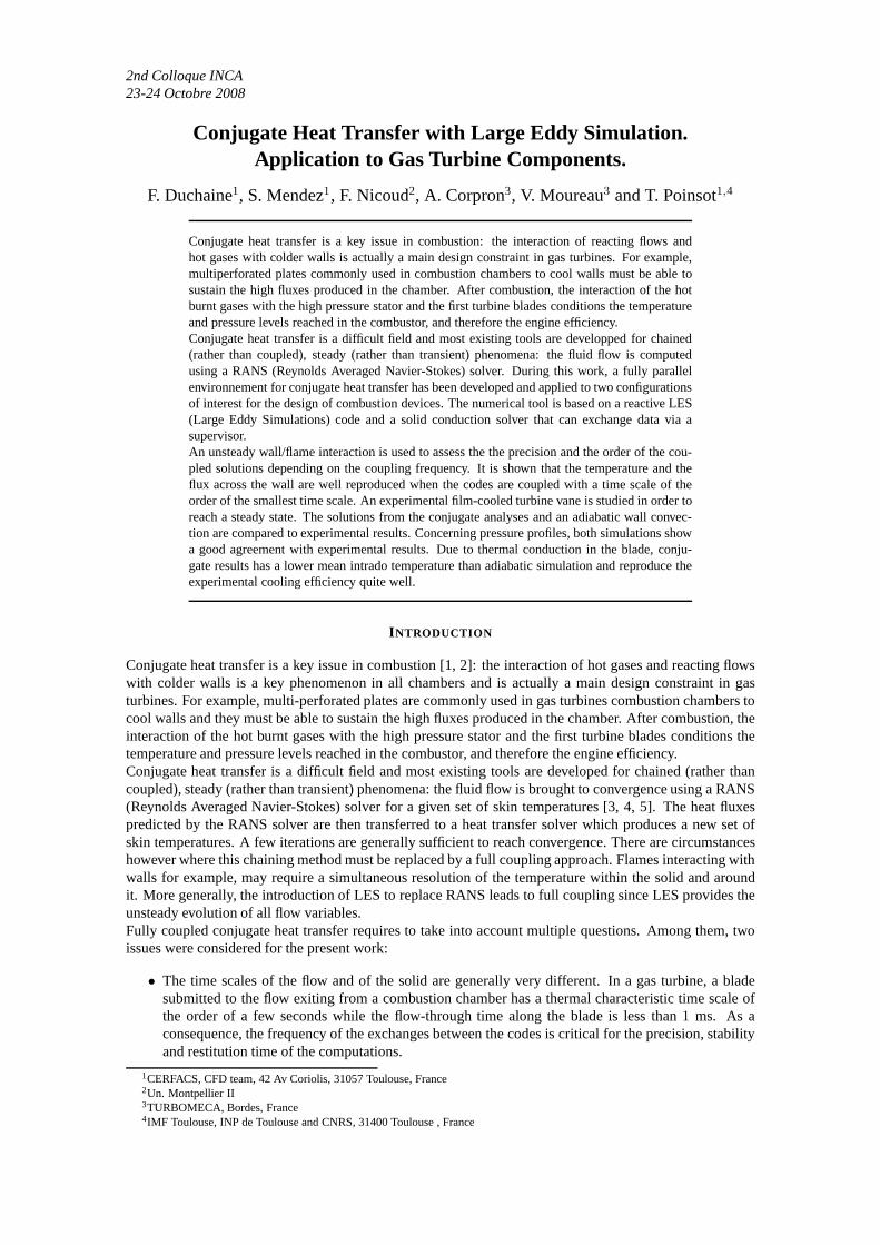
• Synchronization in CPU time: on a parallel machine, codes for the fluid and for the structure may berun together or sequentially. An interesting question controlled by the execution mode is the infor-mation exchange. Fig. 1 shows how heat fluxes and temperatureare exchanged in a mode called SCS(Sequential Coupling Strategy) where the fluid solver afterrun n (physical durationαfτf ) providesfluxes to the solid solver which then starts and gives temperaturesTn (physical durationαsτs). InSCS mode, the codes are loaded into the parallel machine sequentially and each solver use all avail-able processors (N ). Another solution is Parallel Coupling Strategy (PCS) where both solvers runtogether using information obtained from the other solver at the previous coupling iteration (Fig. 1).In this case, the two solvers must share theP = Ps + Pf processors. ThePs andPf processorsdedicated to the solid and the fluid respectively must be suchthat:

Pf

P=

1

1 + Ts/Tf

(1)

whereTs andTf are the execution times of the solid and fluid solvers respectively (on one processor).Ts andTf depend onαsτs andαfτf . Perfect scaling for both solvers is assumed here.

Note that both SCS and PCS questions are linked to the way information (heat fluxes and wall temperatures)are exchanged and to the implementation on parallel machines but are independent of the synchronizationin physical time: PCS or SCS can be used for steady or unsteadycomputations. This paper focuses on thePCS strategy.Finally,this work explores the simplest coupling method where the fluid solver provides heat fluxes to thesolid solver while the solid solver sends skin temperaturesback to the fluid code. More sophisticatedmethods may be used for precision and stability [12, 13] but the present one was found sufficient for thetwo test cases described below.

5For example, when a steady state solution is sought (i.e. to be used as initial condition for an unsteady computation), physicaltimes for both solvers can differ.

2nd Colloque INCA23-24 Octobre 2008

Sequential coupling strategy SCS Parallel coupling strategy PCS

Figure 1 : Main types of coupling strategies.

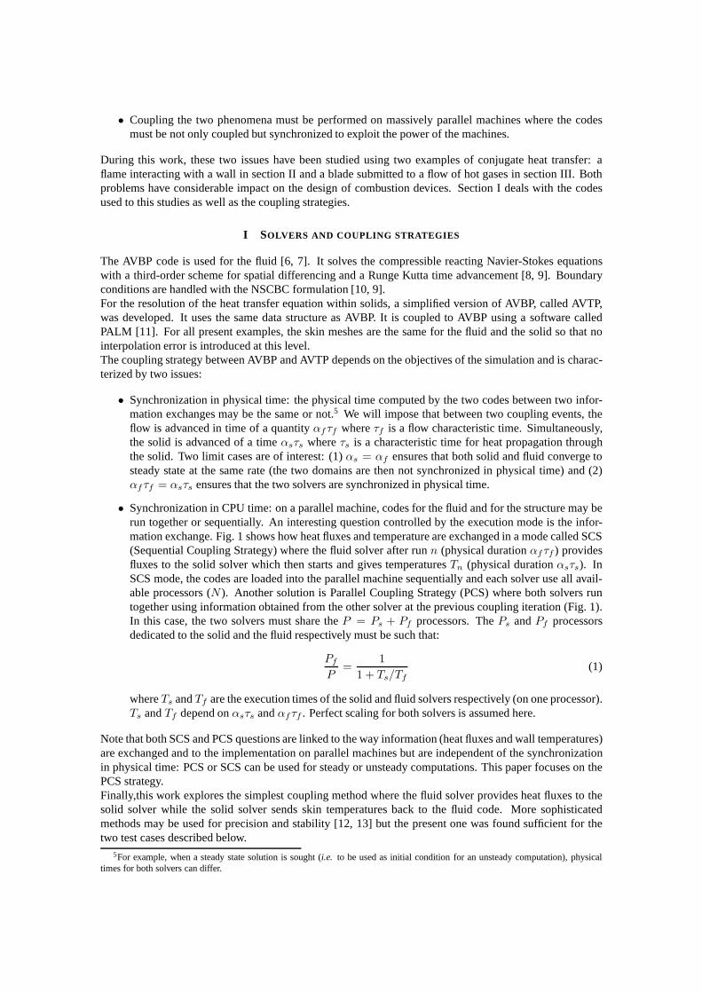
Figure 2 : Interaction between wall and premixed flame. Solid line: initial temperature profile.

II FLAME/WALL INTERACTION (FWI)

The interaction between flames and walls controls combustion, pollution and wall heat fluxes in a significantmanner [10, 14, 15]. It also determines the wall temperatureand its life time. In most combustion devices,burnt gases reach temperatures between1500 and2500 K while walls temperatures remain between400and850 K because of cooling. The temperature decrease from burnt gases levels to wall levels occurs in anear-wall layer which is less than1 mm thick, creating large temperature gradients.Studying the interaction between flames and walls is difficult from an experimental point of view because allinteresting phenomena occur in a thin zone near the wall: in most cases, the only measurable quantity is theunsteady heat flux through the wall. Moreover, flames approaching walls are dominated by transient effects:they usually do not ’touch’ walls and quench a few micrometers away from the cold wall because the lowwall temperature inhibits chemical reactions. At the same time, the large near-wall temperature gradientslead to very high wall heat fluxes. These fluxes are maintainedfor short durations and their characterizationis also a difficult task in experiments [16, 17].The present study focuses on the interaction between a laminar flame and a wall (Fig. 2). Except for afew studies using integral methods within the solid [18] or catalytic walls [19, 20], most studies dedicatedto FWI were performed assuming an inert wall at constant walltemperature. Here we will revisit theassumption of isothermicity of the wall during the interaction.

II.1 THE INFINITELY FAST FLAME (IFF) LIMIT

Flame front thicknesses (δoL) are less than1 mm and laminar flame speeds (so

L) are of the order of1 m/s.Walls are usually made of metal or ceramics and their characteristic time scaleτs = L2/Ds (whereL is thewall thickness andDs the wall diffusivity) is much longer than the flame characteristic time τ = δo

L/soL.

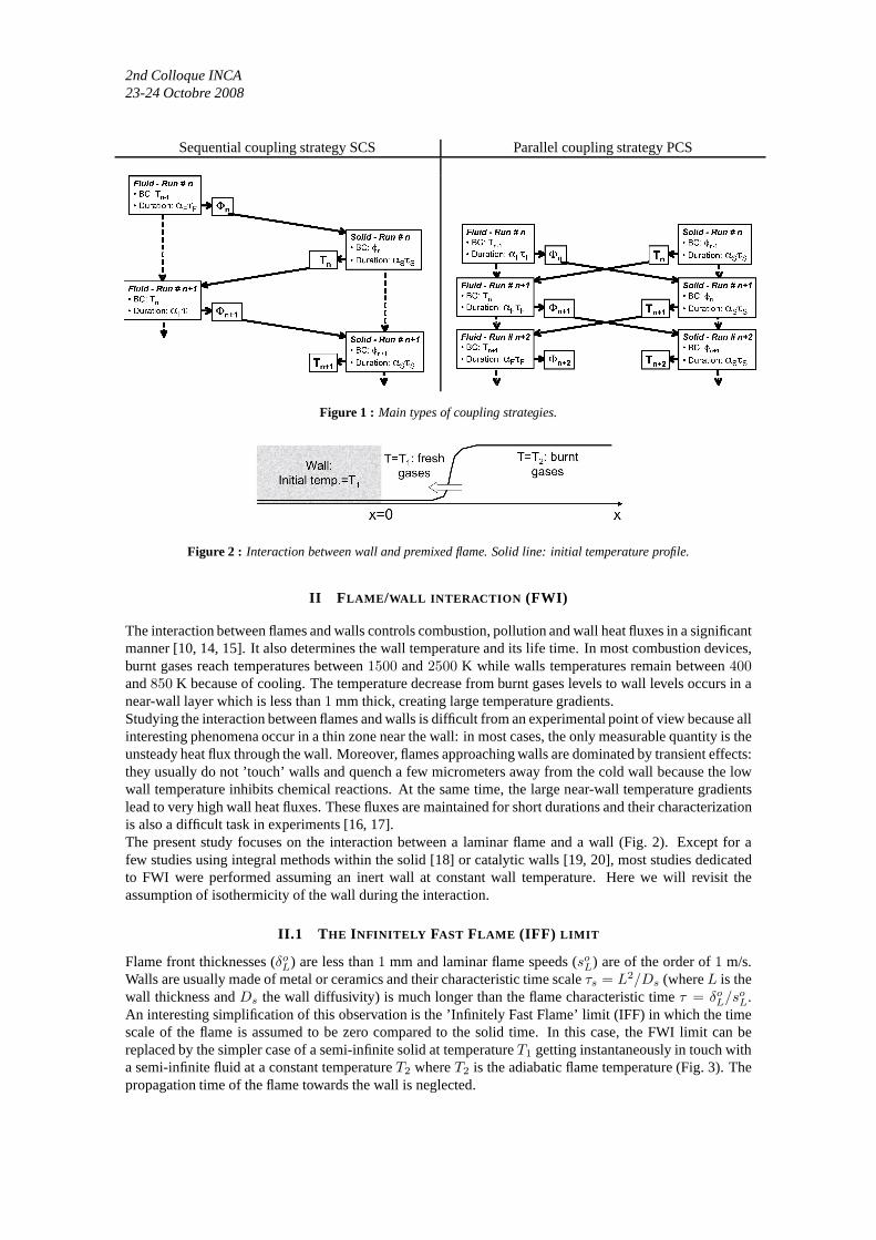
An interesting simplification of this observation is the ’Infinitely Fast Flame’ limit (IFF) in which the timescale of the flame is assumed to be zero compared to the solid time. In this case, the FWI limit can bereplaced by the simpler case of a semi-infinite solid at temperatureT1 getting instantaneously in touch witha semi-infinite fluid at a constant temperatureT2 whereT2 is the adiabatic flame temperature (Fig. 3). Thepropagation time of the flame towards the wall is neglected.

Figure 3 : The IFF (infinitely fast flame) limit. Solid line: initial temperature profile.

Initial Thermal Thermal Thermal Heat Density Mesh Fouriertemperature diffusivity effusivity conductivity capacity size time step

Solid 650 3.38 10−6 7058.17 12.97 460 8350 4 10−6 2.37 10−6

Fluid 660 2.53 10−5 5.52 0.028 1162.2 0.947 4 10−6 3.16 10−7

Table 1 : Fluid and solid characteristics for IFF test case (SI units). The Fourier time step corresponds to the stabilitylimit for explicit schemes∆tD = ∆x2/(2Dth).

The IFF problem is a classical heat transfer problem and has an analytical solution which can be written as:

T (x, t) = T1 + bT2 − T1

b + bs

erfc(−x

2√

Dst) for x < 0 (2)

T (x, t) = T2 − bs

T2 − T1

b + bs

erfc(x

2√

Dt) for x > 0 (3)

whereb =√

λρCp is the effusivity of the burnt gases,bs =√

λsρsCps the effusivity of the wall andD theburnt gases diffusivity .Ds andD are assumed to be constant in the solid and fluid parts. The temperatureof the wall atx = 0 is constant and the heat fluxΦ decreases like1/

√t:

T (x = 0, t) =bT2 + bsT1

b + bs

and Φ(x = 0, t) =T2 − T1

b + bs

bbs√

πt(4)

This IFF limit is useful to understand FWI limits. It was alsoused as a test case of the coupled codes tocheck the accuracy of coupling strategies (next section).

II.2 THE IFF LIMIT AS A TEST CASE FOR UNSTEADY FLUID / HEAT TRANSFER COUPLING

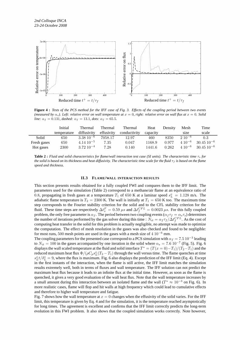
A central question for SCS or PCS methods is the coupling frequency between the two solvers especiallywhen they have very different characteristic times. Since the IFF has an analytical solution, it was first usedas a test case for PCS methods. The test case corresponds to a wall at650 K in contact att = 0 with a fluidat660 K. Compared to a wall/flame interaction, this small temperature difference is chosen in order to keepconstant values forD, λ andCp. Table 1 summarizes the properties of the solid and the fluid and indicatesmesh size∆x and maximum time steps∆tD for diffusion (the only important ones here since the flow doesnot move).The most interesting part of this problem is the initial phase when fluxes are large and coupling difficult.During this phase, the solid and the fluid can be considered asinfinite and there is no proper length or timescale to evaluateτf or τs in Fig. 1. The only useful scale is the grid mesh and the associated time scale forexplicit algorithm stability. Therefore we chose to takeτf = ∆tDf andτs = ∆tDs (Note that the fluid solveris limited by an acoustic time step smaller than∆tDf ). The strategy used for this test is the PCS method(Fig. 1) for unsteady cases which requiresαfτf = αsτs . The αf parameter defines the time intervalbetween two coupling events normalized by the fluid characteristic time. Values ofαf ranging from0.131to 65.5 were tested for this problem and Fig. 4 shows how the errors onmaximum wall temperature and thewall heat flux change whenαf changes. The IFF solution 4 is used as the reference solution. Using valuesof αf larger than unity leads to relative errors which can be significant and to strong oscillations on thetemperature and flux. As expected a full coupling of fluid and solid for this problem requires to use valuesof αf of order unity which means to couple the codes on a time scale which is of the order of the smallesttime scale (here the flow time scale).

2nd Colloque INCA23-24 Octobre 2008

0 100 200 300 400

-1e-05

-5e-06

0e+00

5e-06

Reduced timet+ = t/τf

Rel

ativ

eer

ror

on

tem

per

atu

re

0 100 200 300 400-1

-0.5

0

0.5

1

1.5

Reduced timet+ = t/τf

Rel

ativ

eer

ror

on

flux

Figure 4 : Tests of the PCS method for the IFF case of Fig. 3. Effects of the coupling period between two events(measured byαs). Left: relative error on wall temperature atx = 0, right: relative error on wall flux atx = 0. Solidline: αf = 0.131, dashed:αf = 13.1, dots:αf = 65.5.

Initial Thermal Thermal Thermal Heat Density Mesh Timetemperature diffusivity effusivity conductivity capacity size scale

Solid 650 3.38 10−6 7058.17 12.97 460 8350 2 10−6 0.3Fresh gases 650 4.14 10−5 7.35 0.047 1168.9 0.977 4 10−6 30.45 10−6

Hot gases 2300 3.72 10−4 7.28 0.140 1441.6 0.262 4 10−6 30.45 10−6

Table 2 : Fluid and solid characteristics for flame/wall interactiontest case (SI units). The characteristic timeτs forthe solid is based on its thickness and heat diffusivity. Thecharacteristic time scale for the fluidτf is based on the flamespeed and thickness.

II.3 FLAME/WALL INTERACTION RESULTS

This section presents results obtained for a fully coupled FWI and compares them to the IFF limit. Theparameters used for the simulation (Table 2) correspond to amethane/air flame at an equivalence ratio of0.8, propagating in fresh gases at a temperatureT1 of 650 K at a laminar speedso

L = 1.128 m/s. Theadiabatic flame temperature isT2 = 2300 K. The wall is initially atT1 = 650 K too. The maximum timestep corresponds to the Fourier stability criterion for thesolid and to the CFL stability criterion for thefluid. These time steps are respectively∆tFs = 0.59 µs and∆tCFL

f = 0.0023 µs. For this fully coupledproblem, the only free parameter isαf . The period between two coupling events (αfτf = αsτs) determinesthe number of iterations performed by the gas solver during this time :Nit = αfτf/∆tCFL

f . As the cost ofcomputing heat transfer in the solid for this problem is actually negligible, no attempt was made to optimizethe computation. The effect of mesh resolution in the gases was also checked and found to be negligible:for most runs,500 mesh points are used in the gases with a mesh size of4 10−6 mm.The coupling parameters for the presented case correspond to a PCS simulation withαf = 7.5 10−3 leadingto Nit = 100 in the gases accompanied by one iteration in the solid whereαs = 7.6 10−7 (Fig. 5). Fig. 6displays the wall scaled temperature at the fluid and solid interfaceT ∗ = (T (x = 0)−T1)/(T2−T1) and thereduced maximum heat fluxΦ/(ρCps

oL(T2 −T1) through the wall versus time. The flame quenches at time

soLt/δo

L = 9, where the flux is maximum. Fig. 6 also displays the prediction of the IFF limit (Eq. 4). Exceptin the first instants of the interaction, when the flame is still active, the IFF limit matches the simulationresults extremely well, both in terms of fluxes and wall temperature. The IFF solution can not predict themaximum heat flux because it leads to an infinite flux at the initial time. However, as soon as the flame isquenched, it gives a very good evaluation of the wall heat flux. Note that the wall temperature increases bya small amount during this interaction between an isolated flame and the wall (T ∗ ≈ 10−3 on Fig. 6). Inmore realistic cases, flame will flop and hit walls at high frequency which could lead to cumulative effectsand therefore to higher wall temperature and fatigue.Fig. 7 shows how the wall temperature atx = 0 changes when the effusivity of the solid varies. For the IFFlimit, this temperature is given by Eq. 4 and for the simulation, it is the temperature reached asymptoticallyfor long times. The agreement is excellent and confirms that the IFF limit correctly predicts the long-termevolution in this FWI problem. It also shows that the coupledsimulation works correctly. Note however,

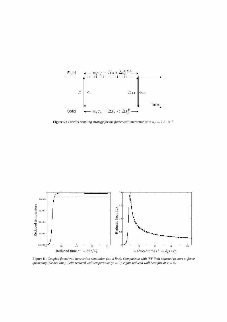
Figure 5 : Parallel coupling strategy for the flame/wall interaction with αf = 7.5 10−3.

0 20 40 60 800.0e+00

2.5e-04

5.0e-04

7.5e-04

1.0e-03

Reduced timet+ = δoLt/so

L

Red

uce

dte

mp

erat

ure

0 20 40 60 800

0.1

0.2

0.3

0.4

Reduced timet+ = δoLt/so

L

Red

uce

dh

eatfl

ux

Figure 6 : Coupled flame/wall interaction simulation (solid line). Comparison with IFF limit adjusted to start at flamequenching (dashed line). Left: reduced wall temperature (x = 0), right: reduced wall heat flux atx = 0.

2nd Colloque INCA23-24 Octobre 2008

100 1000 10000 1e+05 1e+060

0.005

0.01

0.015

0.02

0.025

0.03

Wall effusivityR

edu

ced

tem

per

atu

re

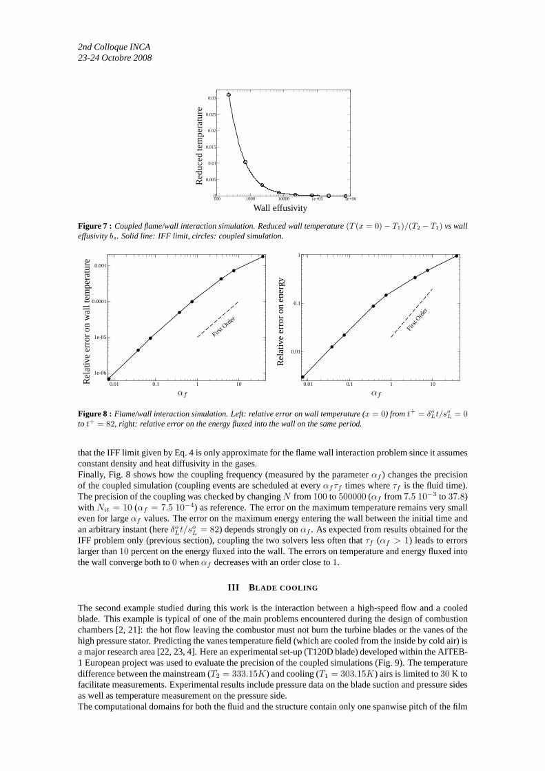
Figure 7 : Coupled flame/wall interaction simulation. Reduced wall temperature(T (x = 0) − T1)/(T2 − T1) vs walleffusivitybs. Solid line: IFF limit, circles: coupled simulation.

0.01 0.1 1 10

1e-06

1e-05

0.0001

0.001

First O

rder

αf

Rel

ativ

eer

ror

on

wal

ltem

per

atu

re

0.01 0.1 1 10

0.01

0.1

1

Firs

t Ord

er

αf

Rel

ativ

eer

ror

on

ener

gy

Figure 8 : Flame/wall interaction simulation. Left: relative error on wall temperature (x = 0) from t+ = δoLt/so

L = 0to t+ = 82, right: relative error on the energy fluxed into the wall on the same period.

that the IFF limit given by Eq. 4 is only approximate for the flame wall interaction problem since it assumesconstant density and heat diffusivity in the gases.Finally, Fig. 8 shows how the coupling frequency (measured by the parameterαf ) changes the precisionof the coupled simulation (coupling events are scheduled ateveryαf τf times whereτf is the fluid time).The precision of the coupling was checked by changingN from 100 to 500000 (αf from 7.5 10−3 to 37.8)with Nit = 10 (αf = 7.5 10−4) as reference. The error on the maximum temperature remainsvery smalleven for largeαf values. The error on the maximum energy entering the wall between the initial time andan arbitrary instant (hereδo

Lt/soL = 82) depends strongly onαf . As expected from results obtained for the

IFF problem only (previous section), coupling the two solvers less often thatτf (αf > 1) leads to errorslarger than10 percent on the energy fluxed into the wall. The errors on temperature and energy fluxed intothe wall converge both to0 whenαf decreases with an order close to1.

III BLADE COOLING

The second example studied during this work is the interaction between a high-speed flow and a cooledblade. This example is typical of one of the main problems encountered during the design of combustionchambers [2, 21]: the hot flow leaving the combustor must not burn the turbine blades or the vanes of thehigh pressure stator. Predicting the vanes temperature field (which are cooled from the inside by cold air) isa major research area [22, 23, 4]. Here an experimental set-up (T120D blade) developed within the AITEB-1 European project was used to evaluate the precision of the coupled simulations (Fig. 9). The temperaturedifference between the mainstream (T2 = 333.15K) and cooling (T1 = 303.15K) airs is limited to30 K tofacilitate measurements. Experimental results include pressure data on the blade suction and pressure sidesas well as temperature measurement on the pressure side.The computational domains for both the fluid and the structure contain only one spanwise pitch of the film

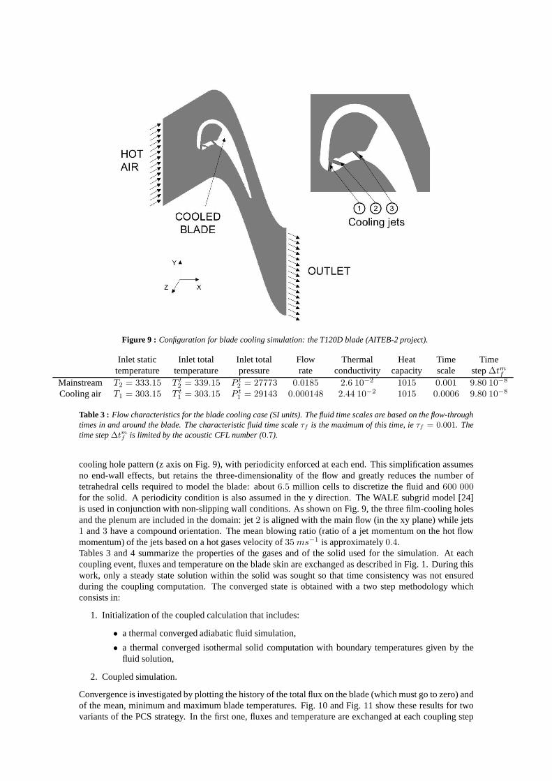
Figure 9 : Configuration for blade cooling simulation: the T120D blade(AITEB-2 project).

Inlet static Inlet total Inlet total Flow Thermal Heat Time Timetemperature temperature pressure rate conductivity capacity scale step∆tmf

Mainstream T2 = 333.15 T t2 = 339.15 P t

2 = 27773 0.0185 2.6 10−2 1015 0.001 9.80 10−8

Cooling air T1 = 303.15 T t1 = 303.15 P t

1 = 29143 0.000148 2.44 10−2 1015 0.0006 9.80 10−8

Table 3 : Flow characteristics for the blade cooling case (SI units).The fluid time scales are based on the flow-throughtimes in and around the blade. The characteristic fluid time scaleτf is the maximum of this time, ieτf = 0.001. Thetime step∆tm

f is limited by the acoustic CFL number (0.7).

cooling hole pattern (z axis on Fig. 9), with periodicity enforced at each end. This simplification assumesno end-wall effects, but retains the three-dimensionalityof the flow and greatly reduces the number oftetrahedral cells required to model the blade: about6.5 million cells to discretize the fluid and600 000for the solid. A periodicity condition is also assumed in they direction. The WALE subgrid model [24]is used in conjunction with non-slipping wall conditions. As shown on Fig. 9, the three film-cooling holesand the plenum are included in the domain: jet2 is aligned with the main flow (in the xy plane) while jets1 and3 have a compound orientation. The mean blowing ratio (ratio of a jet momentum on the hot flowmomentum) of the jets based on a hot gases velocity of35 ms−1 is approximately0.4.Tables 3 and 4 summarize the properties of the gases and of thesolid used for the simulation. At eachcoupling event, fluxes and temperature on the blade skin are exchanged as described in Fig. 1. During thiswork, only a steady state solution within the solid was sought so that time consistency was not ensuredduring the coupling computation. The converged state is obtained with a two step methodology whichconsists in:

1. Initialization of the coupled calculation that includes:

• a thermal converged adiabatic fluid simulation,

• a thermal converged isothermal solid computation with boundary temperatures given by thefluid solution,

2. Coupled simulation.

Convergence is investigated by plotting the history of the total flux on the blade (which must go to zero) andof the mean, minimum and maximum blade temperatures. Fig. 10and Fig. 11 show these results for twovariants of the PCS strategy. In the first one, fluxes and temperature are exchanged at each coupling step

2nd Colloque INCA23-24 Octobre 2008

Thermal Heat Density Thermal Time Timeconductivity capacity diffusivity scaleτs step

0.184 1450 1190 1.07 10−7 34.22 1.71 10−3

Table 4 : Solid characteristics for the blade cooling case (SI units). The time scaleτs is computed using the thermaldiffusivity and the blade minimum thickness.

0 1 2 3 4 5 6 7 8200

225

250

275

300

325

350

375

400

Reduced timet+ = t/τs

Tem

per

atu

re

0 1 2 3 4 5 6 7 8

0

1

2

3

Reduced timet+ = t/τs

Tota

lwal

lflu

x

Figure 10 : Time evolution of minimum and maximum temperatures in the blade (left) and total heat flux through theblade with (solid) and without (dashed) relaxation.

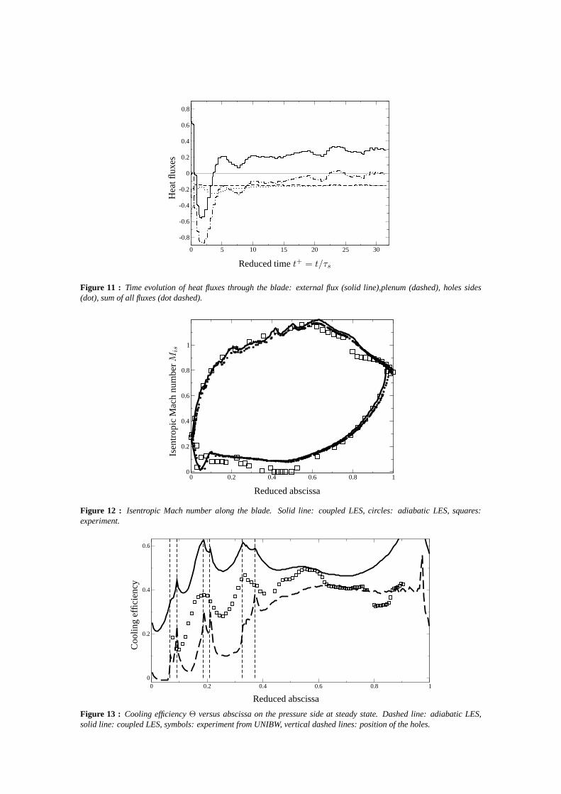
while for the second one, relaxation is used and temperatureand fluxes imposed at each coupling iterationn are written asfn = afn−1 + (1 − a)fn∗ wherefn∗ is the value obtained by the other solver at iterationn anda is a relaxation factor (typicallya = 0.6). Without relaxation, the system becomes unstable andconvergence almost impossible.At the converged state, the total flux reaches zero: the flux entering the blade is evacuated into the coolingair in the plenum and in the holes (Fig. 11). Note however thatthe analysis of fluxes on the blade skinshows that, even though the blade is heated by the flow on the pressure side, it is actually cooled on partof the suction side because the flow accelerates and cools down on this side. Due to the acceleration in thejets, heat transfer in the holes and plenum are of the same order. Compared to the external flux, plenum andhole fluxes converge almost linearly. Oscillations in the external flux evolution are linked with the complexflow structure developing around the blade.At the converged state, results can be compared to the experiment in terms of pressure profiles on the blade(on both sides) and of temperature profiles on the pressure side. Pressure fields are displayed in terms ofisentropic Mach numbersMis computed by

Mis =

√

√

√

√

2

γ − 1

[

(

P t2

P tw

)

γ−1

γ

− 1

]

(5)

whereP t2 andP t

w are the total pressure of the main stream and at the wall. Fig.12 displays an averagefield of isentropic Mach number obtained by LES and by the experiment. The comparison of the adiabaticsimulation and the coupled one shows that these profiles are only weakly sensitive to the thermal conditionimposed on the blade. Although the shock position on the suction side is not perfectly captured, the overallagreement between LES and experimental results is fair.Temperature results are displayed in terms of reduced temperatureΘ = (T t

2 − T )/(T t2 −T t

1) whereT t2 and

T t1 are the total temperatures of the main and cooling streams (Table 4) andT is the local wall temperature.

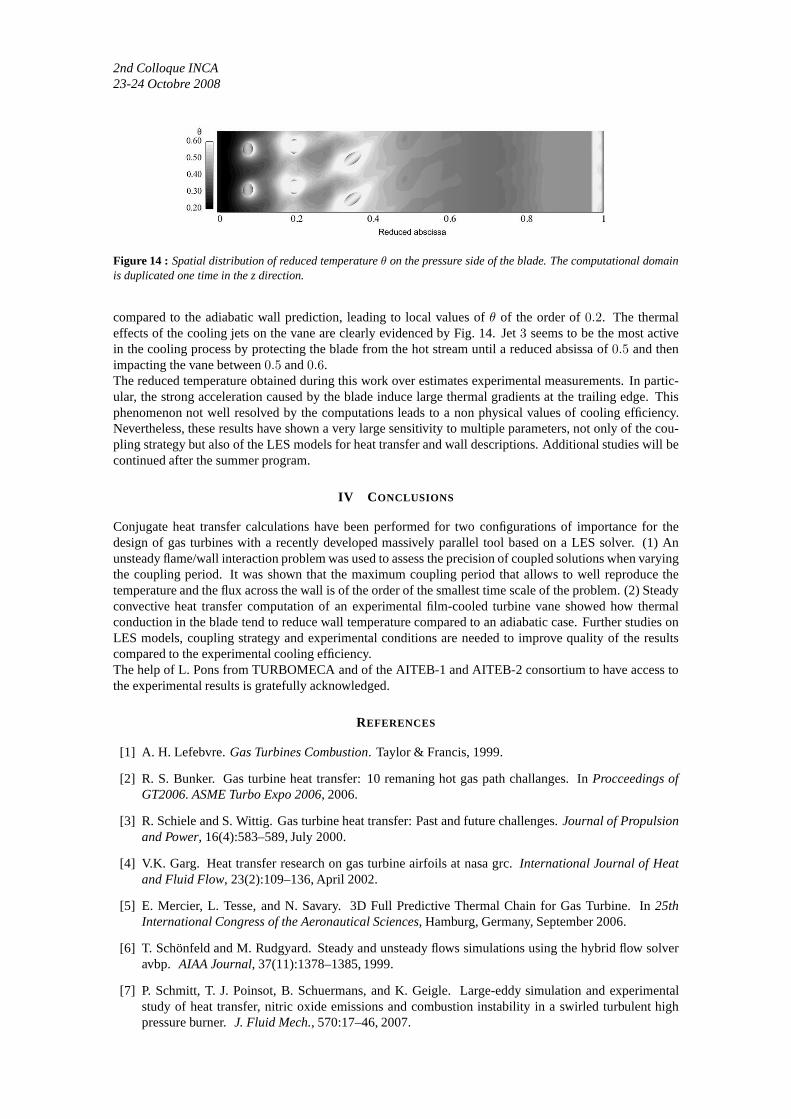
Θ measures the cooling efficiency of the blade. Fig. 13 shows measurements, adiabatic and coupled LESresults forΘ spanwise averaged along axis x. As expected, the cooling efficiency obtained with the adiabaticcomputation are lower than the experimental values: the adiabatic temperature field over-predicts the realone. The main contribution of conduction in the blade is to reduce the wall temperature on the pressureside.The reduced temperature distribution on the pressure side (Fig. 14) shows that the peak temperature occursat the stagnation point (reduced abscissa close to0). The temperature at the stagnation point is reduced

0 5 10 15 20 25 30

-0.8

-0.6

-0.4

-0.2

0

0.2

0.4

0.6

0.8

Reduced timet+ = t/τs

Hea

tflu

xes

Figure 11 : Time evolution of heat fluxes through the blade: external flux(solid line),plenum (dashed), holes sides(dot), sum of all fluxes (dot dashed).

0 0.2 0.4 0.6 0.8 10

0.2

0.4

0.6

0.8

1

Reduced abscissa

Isen

tro

pic

Mac

hn

um

berM

is

Figure 12 : Isentropic Mach number along the blade. Solid line: coupledLES, circles: adiabatic LES, squares:experiment.

0 0.2 0.4 0.6 0.8 10

0.2

0.4

0.6

Reduced abscissa

Co

olin

gef

ficie

ncy

Figure 13 : Cooling efficiencyΘ versus abscissa on the pressure side at steady state. Dashedline: adiabatic LES,solid line: coupled LES, symbols: experiment from UNIBW, vertical dashed lines: position of the holes.

2nd Colloque INCA23-24 Octobre 2008

Figure 14 : Spatial distribution of reduced temperatureθ on the pressure side of the blade. The computational domainis duplicated one time in the z direction.

compared to the adiabatic wall prediction, leading to localvalues ofθ of the order of0.2. The thermaleffects of the cooling jets on the vane are clearly evidencedby Fig. 14. Jet3 seems to be the most activein the cooling process by protecting the blade from the hot stream until a reduced absissa of0.5 and thenimpacting the vane between0.5 and0.6.The reduced temperature obtained during this work over estimates experimental measurements. In partic-ular, the strong acceleration caused by the blade induce large thermal gradients at the trailing edge. Thisphenomenon not well resolved by the computations leads to a non physical values of cooling efficiency.Nevertheless, these results have shown a very large sensitivity to multiple parameters, not only of the cou-pling strategy but also of the LES models for heat transfer and wall descriptions. Additional studies will becontinued after the summer program.

IV CONCLUSIONS

Conjugate heat transfer calculations have been performed for two configurations of importance for thedesign of gas turbines with a recently developed massively parallel tool based on a LES solver. (1) Anunsteady flame/wall interaction problem was used to assess the precision of coupled solutions when varyingthe coupling period. It was shown that the maximum coupling period that allows to well reproduce thetemperature and the flux across the wall is of the order of the smallest time scale of the problem. (2) Steadyconvective heat transfer computation of an experimental film-cooled turbine vane showed how thermalconduction in the blade tend to reduce wall temperature compared to an adiabatic case. Further studies onLES models, coupling strategy and experimental conditionsare needed to improve quality of the resultscompared to the experimental cooling efficiency.The help of L. Pons from TURBOMECA and of the AITEB-1 and AITEB-2 consortium to have access tothe experimental results is gratefully acknowledged.

REFERENCES

[1] A. H. Lefebvre.Gas Turbines Combustion. Taylor & Francis, 1999.

[2] R. S. Bunker. Gas turbine heat transfer: 10 remaning hot gas path challanges. InProcceedings ofGT2006. ASME Turbo Expo 2006, 2006.

[3] R. Schiele and S. Wittig. Gas turbine heat transfer: Pastand future challenges.Journal of Propulsionand Power, 16(4):583–589, July 2000.

[4] V.K. Garg. Heat transfer research on gas turbine airfoils at nasa grc.International Journal of Heatand Fluid Flow, 23(2):109–136, April 2002.

[5] E. Mercier, L. Tesse, and N. Savary. 3D Full Predictive Thermal Chain for Gas Turbine. In25thInternational Congress of the Aeronautical Sciences, Hamburg, Germany, September 2006.

[6] T. Schönfeld and M. Rudgyard. Steady and unsteady flows simulations using the hybrid flow solveravbp. AIAA Journal, 37(11):1378–1385, 1999.

[7] P. Schmitt, T. J. Poinsot, B. Schuermans, and K. Geigle. Large-eddy simulation and experimentalstudy of heat transfer, nitric oxide emissions and combustion instability in a swirled turbulent highpressure burner.J. Fluid Mech., 570:17–46, 2007.

[8] O. Colin and M. Rudgyard. Development of high-order taylor-galerkin schemes for unsteady calcula-tions. J. Comput. Phys., 162(2):338–371, 2000.

[9] V. Moureau, G. Lartigue, Y. Sommerer, C. Angelberger, O.Colin, and T. Poinsot. High-order meth-ods for DNS and LES of compressible multi-component reacting flows on fixed and moving grids.J. Comput. Phys., 202(2):710–736, 2005.

[10] T. Poinsot and D. Veynante.Theoretical and numerical combustion. R.T. Edwards, 2nd edition., 2005.

[11] S. Buis, A. Piacentini, and D. Déclat. PALM: A Computational Framework for assembling HighPerformance Computing Applications.CONCURRENCY AND COMPUTATION: PRACTICE ANDEXPERIENCE, 2005.

[12] M.B. Giles. Stability analysis of numerical interfaceconditions in fluid-structure thermal analysis.International Journal for Numerical Methods in Fluids, 25(4):421–436, 1997.

[13] S. Chemin.Étude des Interactions Thermiques Fluides-Structure par un Couplage de Codes de Cal-cul. PhD thesis, Université de Reims Champagne-Ardenne, 2006.

[14] A. Delataillade, F. Dabireau, B. Cuenot, and T. Poinsot. Flame/wall interaction and maximum heatwall fluxes in diffusion burners.Proc. Combust. Inst., 29:775–780, 2002.

[15] F. Dabireau, B. Cuenot, O. Vermorel, and T. Poinsot. Interaction of h2/o2 flames with inert walls.Combust. Flame, 135(1-2):123–133, 2003.

[16] J. H. Lu, O. Ezekoye, R. Greif, and F. Sawyer. Unsteady heat transfer during side wall quenchingof a laminar flame. In23rd Symp. (Int.) on Combustion, pages 441–446. The Combustion Institute,Pittsburgh, 1990.

[17] O. A. Ezekoye, R. Greif, and D. Lee. Increased surface temperature effects on wall heat transfer duringunsteady flame quenching. In24th Symp. (Int.) on Combustion, pages 1465–1472. The CombustionInstitute, Pittsburgh, 1992.

[18] G. Desoutter, B. Cuenot, C. Habchi, and T. Poinsot. Interaction of a premixed flame with a liquid fuelfilm on a wall. Proc. Combust. Inst., 30:259–267, 2005.

[19] P. Popp, M. Baum, M. Hilka, and T. Poinsot. A numerical study of laminar flame wall interactionwith detailed chemistry: wall temperature effects. In T. J.Poinsot, T. Baritaud, and M. Baum, edi-tors,Rapport du Centre de Recherche sur la Combustion Turbulente, pages 81–123. Technip, RueilMalmaison, 1996.

[20] P. Popp and M. Baum. An analysis of wall heat fluxes, reaction mechanisms and unburnt hydrocarbonsduring the head-on quenching of a laminar methane flame.Combust. Flame, 108(3):327 – 348, 1997.

[21] D. G. Bogard and K. A. Thole. Gas turbine film cooling.J. Prop. Power, 22(2):249–270, 2006.

[22] M.-L. Holmer, L.-E. Eriksson, and B. Sunden. Heat transfer on a film cooled inlet guide vane. InProceedings of the ASME Heat Transfer Division, volume 366-3, pages 43–50, 2000.

[23] G. Medic and P. A. Durbin. Toward improved film cooling prediction. J. Turbomach., 124:193–199,2002.

[24] F. Nicoud and T. Poinsot. Dns of a channel flow with variable properties. InInt. Symp. On Turbulenceand Shear Flow Phenomena., Santa Barbara, Sept 12-15., 1999.