ieulletin of the t Fisheries Research Rnrri of...

HYDRODYNAMICS AND ENERGETICS OF FISH PROPULSION

— . W. WEBB

1141 Can Fish

223 138 21 3 no. 190 JC

LETIN 190 a 1975

ENVttt .

' 3

JL aw

e

ieulletin of the , t Fisheries Research Rnrri of CanactT

DFO Lb a y MPO B bliotheque

Ill 11 11111 11 1111 11 11 12039430

Historical Resumé

6th Century B.C. First reference to propulsive function of the tail.

1680 G. A. Borelli compared movements of the caudal fin to an oar.

1873 J. B. Pettigrew observed shape of the propulsive wave.

1895 E. J. Marey used cinephotography to study locomotorykinematics of swimming fish.

1912 S. F. Houssay attempted to measure thrust and drag of fish.

1926 C. M. Breder summarized and classified types of propulsivemovements in fish.

1933 Sir James Gray showed how propulsive movements generatethrust, and defined kinematic conditions required.

1936 Sir James Gray used hydrodynamic theory of drag for rigidbodies of revolution to calculate drag of a swimmingdolphin, and compared this with the then best knownvalues for mammalian muscle power output. Insufficientpower output was available to overcome the theoreticallyexpected hydrodynamic drag - Gray's Paradox.

1938, 1939 A. V. Hill used direct calorimetry to determine powercharacteristics for contracting vertebrate muscle.

1952 Sir Geoffrey Taylor used hydrofoil theory to formulate aquantitative hydrodynamic model for fish propulsion.

1961 R. Bainbridge used hydrodynamic theory for drag of rigidbodies of revolution as a model for the swimmingdrag of fish and cetaceans; drag was compared with thelatest values for muscle power output. Gray's Paradoxnot supported for most fish or cetaceans. M. F. M.Osborne used the same hydrodynamic theory, and com-pared drag of migrating salmon with power expended,as determined by indirect calorimetry. Insufficient powerwas available to overcome hydrodynamic drag.

HYDRODYNAMICS

AND ENERGETICS

OF FISH PROPULSION

Bulletins are designed to interpret current knowledge in scientific fields pertinent to Canadian fisheries and aquatic environments. Recent numbers in this series are listed at the back of this Bulletin.

The Journal of the Fisheries Research Board of Canada is published in annual volumes of monthly issues and Miscellaneorts —SPecial Publications are issued periodically. -Tfies—e—Seffl- are-. for sale by information Canada, Ottawa, KlA 0S9. Remittances must be in advance, payable in Canadian funds to the order of the Receiver General of Canada.

Les bulletins sont conçus dans le but d'évaluer et d'interpréter les connaissances actuelles dans les domaines scientifiques qui se rapportent aux pêches et à l'environnement aquatique du Canada. On trouvera une liste des récents bulletins à la fin de la présente publication.

Le Journal of the Fisheries Research Board of Canada est publié en volumes annuels de douze numéros et les Publications diverses spéciales sont publiées périodiquement. Ces publications sont en vente à la librairie d'Information Canada, Ottawa, K 1 A 0S9. Les remises, payables d'avance en monnaie canadienne, doivent être faites à l'ordre du Receveur général du Canada.

Editor and 'Rédacteur et Director of Scientific Information

Directeur de l'information scientifique

Deputy Editor Sous-rédacteur

Assistant Editors Rédacteurs adjoints

Production Documentation

Bureau du directeur de la publication Service des pêches et des sciences de la mer

Ministère de l'Environnement 116, rue Lisgar, Ottawa, Canada

KlA OH3

J. C. STEVENSON, PH.D.

J. WATSON, PH.D.

R. H. WIGMORE, M.SC. JOHANNA M. REINHART, M.SC.

J. CAMP G. J. NEVILLE/MICKEY LEWIS

Office of the Editor Fisheries and Marine Service Department of the Environment 116 Lisgar Street, Ottawa, Canada KIA OH3

oc

m

~"QAlr.rr:;

BULLETIN 190

Hydrodynamics

and Energetics of Fish Propulsion

PAUL W. WEBB

Department of the Environment Fisheries and Marine Service Pacific Biological Station Nanaimo, B.C.

DEPARTMENT OF THE ENVIRONMENT FISHERIES AND MARINE SERVICE Ottawa 1975

Frontispiece: Edward Mitchell, Department of the Environment, Fisheries and Marine Service, Arctic Biological Station, Ste. Anne de Bellevue, Que.

N o. ( 9

(0) Crown Copyrights reserved Droits de la Couronne réservés

Available by mail from Information Canada, Ottawa, KIA 0S9 and at the following Information Canada bookshops:

En vente chez Information Canada à Ottawa, K1A 0S9 et dans les librairies d'Information Canada:

HALIFAX HALIFAX

1683 Barrington Street 1683, rue Barrington

MONTREAL MONTRÉAL

640 St. Catherine Street West 640 ouest, rue Ste - Catherine

OTTAWA OTTAWA 171 Slater Street 171, rue Slater

TORONTO TORONTO

221 Yonge Street 221, rue Yonge

WINNIPEG WINNIPEG

393 Portage Avenue 393, avenue Portage

VANCOUVER VANCOUVER

800 Granville Street 800, rue Granville

or through your bookseller ou chez votre libraire.

Canada: $5.00 Catalogue No. Fs 94-190 Other countries: $6.00

Price subject to change without notice

Information Canada Ottawa, 1975

Canada: $5.00 N. de catalogue Fs 94-190 Autres pays $6.00

Prix sujet à changement sans avis préalable

Information Canada Ottawa, 1975

Contents

1 ABSTRACT

2 RÉSUMÉ

3 PREFACE

5 INTRODUCTION

PART 1

999

15

18

2222

2424

26

3031

CHAPTER 1. HYDRODYNAMICS

IntroductionSome Physical Properties of Water

DensityViscosity

Methods of Describing FlowPressure and VelocityHydromechanics, Hydraulics, and the Boundary-Layer ConceptLaws of Similitude

Reynolds LawFroudes Law

The Boundary LayerBoundary-Layer ThicknessTransitionCauses of Transition and Separation

Flow and Origin of DragFlow around Circular ProfileStreamline Profile

Vortex Sheets in Perfect FluidsEquations of Drag for Plates and Solid Bodies

Frictional Drag CoefficientPressure Drag Coefficient

Boundary-Layer Flow Conditions and Total DragPeriodic and Unsteady Motion

Periodic MotionUnsteady Motion

HydrofoilsFlow Pattern and ForcesGeometryEquations for Lift and DragCenter of Lift

Note on PropellersFlow Through Pipes

Flow PatternsLaw of Continuity and Bernoulli's TheoremPressure Drop and Resistance to Flow

vii

Contents — Continued PART I — Continued

33 CHAPTER 2. KINEMATICS 33 Classification of Propulsive Movements 35 Body and Caudal Fin Movements

Anguilliform Mode Carangiform Modes Ostraciform Mode

47 Median and Paired Fin Propulsion 48 Concluding Comments

49 CHAPTER 3. SWIMMING SPEEDS

49 Introduction 49 Swimming Levels

Sustained Levels Prolonged Levels Burst Intermediate Levels

51 Swimming Speeds and Size Effects Anguilhform Mode Subcarangiforn2 and Carangiform Modes Carangiform Mode with SemiIrritate Tail Other Swimming Modes

54 Factors Affecting Swimming Speed

57 CHAPTER 4. DRAG 57 Introduction 57 Theoretical Drag 58 Dead Drag

Sources of Error in Dead-Drag Measurements Dead Drag of Fishes

66 Validity of Theoretical and Dead-Drag Measurements 68 Mechanisms to Reduce Drag

Maintenance of Laminar Boundary Layer Reducing Viscosity and Frictional Drag Delay and Prevention of Separation Prevention of Energy Loss as Vorticity Behavioral Mechanisms Discussion

77 CHAPTER 5. THRUST AND POWER • 77 Introduction 77 Direct Measurements of Power Output 78 Hydromechanical Models and Indirect Measurements

Qualitative Quasi-Static Models Quantitative Models

83 Steady Swimming Anguilliform Propulsion Carangiform Modes Carangiform Mode with Semilunate Tail Discussion

viii

Contents - Continued

PART I - Concluded

101 CHAPTER 5. THRUST AND POWER - Conc]uded

101 AccelerationIntroductionKinematicsPower Requirements

105 SUMMARY

PART 2

109

109109

110

113

114

117

121

121121122

125

131

134

135

136

137

CHAPTER 6. METABOLISM AND ENERGY DISTRIBUTION

IntroductionProduction of Biological Energy

Metabolic PathwaysMeasurement of Biological Energy

Bomb CalorimetryIndirect Calorimetry

Metabolic RatesAerobic MetabolismAnaerobic Metabolism-Energy Released

The Muscle SystemRed and White MuscleMuscle Power OutputPower Output and Muscle Shortening Speed

Energy Distribution in the Propulsive SystemAnaerobic Metabolic EnergyAerobic Metabolic Energy

CHAPTER 7. PROPULSION EFFICIENCY

IntroductionDefinitionsEfficiency Studies

Efficiency and Theoretical DragEfficiency and Dead DragEfficiency and Measured PowerEfficiency and Hydromechanical ModelsOptimum Speed

Analysis of Overall EfficienciesKinematicsOxygen ConsumptionEfficiencyThrust and Drag

Discussion

SUMMARY

CLOSING REMARKS

ACKNOWLEDGMENTS

REFERENCES

ix

Contents — Concluded PART II — Concluded

145 APPENDIX I. METHODS

145 Flow Visualization Outer Flow Boundary-Layer Flow

145 Drag Measurements Methods Speed Corrections for Water Tunnels

151 APPENDIX II. SYMBOLS 151 Arabic Symbols 152 Greek Symbols

15 3 SYSTEMATIC INDEX

156 SUBJECT INDEX

X

Abstract

WEBB, P. W. 1974. Hydrodynamics and energetics of fish propulsion. Bull. Fish. Res. Board Can. 190: 159 p.

The object of this monograph is to span the gap between biological and physical science ap-proaches to fish propulsion problems. An attempt is made to summarize and collate the two principal disciplinary approaches as a basis for dialogue and ongoing research.

Principles of hydrodynamics are discussed, oriented to biologists. Following a discussion of kinematics and swimming performance, the hydrodynamic principles are applied in discussing the fundamental problem of drag and thrust. The traditionally employed rigid-body analogy (theoretical drag calculation for equivalent rigid bodies or dead-drag measurements on fish with the body stretched straight) is not considered a valid assumption from which swimming thrust (= drag) power may be computed. Movements made by most fish during swimming are likely to severely distort flow. As a result, the flow around a swimming fish is not likely to be mechanically equivalent to that assumed by the rigid-body analogy.

Alternative methods of calculating thrust power from hydrodynamic models based on the move-ments of swimming fish are discussed. Reaction models developed by Lighthill are considered most appropriate for biological application at present, although no current model is complete. It is likely that a complete model would be too complex for biological application. Problematic measurement or mathematical formulation areas could be incorporated in coefficient form in a semiempirical model. Coefficients could be based on key kinematic parameter modes. Such a semiempirical model is con-sidered a viable alternative to a complete model, and would be particularly suitable for application to field situations in calculating propulsion energy expenditure. Development of both basic models and a semiempirical model is contingent upon further comparative research on propulsion kinematics.

A variety of mechanisms to reduce the drag of swimming fish has been proposed in the literature. Only a few are likely to operate. These include special body shapes in fish that swim with the bulk of the body held fairly straight, distributed dynamic damping in Desmodetna, distributed viscous damping possibly in cetaceans, induction and maintenance of turbulent boundary-layer flow to avoid premature separation, vortex sheets filling fin gaps, and vortex interaction among schooling fish. Mucus may be a universal drag-reducing mechanism among fish.

Principles of biological energy metabolism are discussed oriented to nonbiologists. Biological energetics and mechanics are integrated in a discussion of propulsion efficiency. The use of hydro-mechanical models is supported providing reasonably complete data are available. Efficiency studies emphasize biological areas requiring additional research. These include characteristics, energetics, and division of labor between various muscle systems, contributions of aerobic and anaerobic meta-bolism to total energy expenditure at all activity levels, and energy distribution to propulsion system components.

Discussion is largely restricted to caudal fin and body propulsion at relatively low activity levels. Few data are available for other propulsion modes. A preliminary model is constructed to describe mechanical energy expenditure during acceleration. This suggests that highest final swimming speeds are reached in the shortest time with lowest energy expenditure at highest acceleration rates.

1

Résumé

WEBB, P. W. 1974. Hydrodynamics and energetics of fish propulsion. Bull. Fish. Res. Board Can. 190: 159 p.

L'objectif de cette monographie est de combler le vide entre les disciplines biologique et physique dans l'étude des problèmes de propulsion chez les poissons. L'auteur tente de résumer et d'assembler les méthodes d'attaque des deux principales disciplines en vue de fournir une base au dialogue et à la recherche en cours.

Il discute, à l'intention des biologistes, des principes de l'hydrodynamique. Après une analyse de la cinématique et de la performance de la nage, le problème de la résistance et de la poussée est examiné à la lumière des principes hydrodynamiques. L'analogie traditionnelle du corps rigide (calcul de la résistance théorique pour des corps rigides équivalents, ou mesures de résistance statique sur un poisson dont le corps est étiré et droit) n'est pas considérée comme hypothèse valide pour le calcul de la force de poussée natatoire ( = résistance). Les mouvements exécutés par la majorité des poissons pendant la nage sont de nature à déformer fortement l'écoulement. Comme résultat, il est peu probable que l'écoulement autour d'un poisson qui nage équivaille mécaniquement à celui que laisse supposer l'analogie du corps rigide.

L'auteur examine des variantes pour le calcul de la force de poussée à partir des modèles fondés sur les mouvements de poissons qui nagent. Les modèles à réaction mis au point par Lighthill semblent, pour le moment, les plus appropriés à une application biologique. L'auteur admet qu'aucun des modèles courants n'est complet. De plus, il est probable qu'un modèle complet soit trop compliqué pour application biologique. Des mesures problématiques ou des formules mathématiques pourraient être incorporées, sous forme de coefficients, dans un modèle semi-empirique. Des coefficients pour-raient être établis à partir de paramètres cinématiques de modèles clefs. Un modèle semi-empirique de cette nature est considéré comme alternative viable d'un modèle complet, et qui pourrait être appliqué particulièrement bien à des situations sur le terrain pour le calcul de la dépense d'énergie de propulsion. Le développement, tant des modèles de base que des modèles semi-empiriques, dépend de recherches comparatives plus poussées sur la cinématique de propulsion.

On a suggéré dans la littérature une variété de mécanismes ayant pour fonction de réduire la résistance chez les poissons qui nagent. Quelques-uns seulement sont considérés comme fonctionnels. Parmi ceux-ci, on compte les formes corporelles spéciales de poissons qui nagent avec le plus gros de leur corps maintenu assez droit, l'amortissement dynamique réparti de Desmodema, l'amortissement visqueux réparti possiblement des cétacés, l'induction et le maintien d'un écoulement turbulent aux surfaces de discontinuité afin d'éviter une séparation prématurée, les lames tourbillonnaires remplissant les vides et l'interaction tourbillonnaire entre les poissons d'un banc. Il se peut que le mucus soit un mécanisme universel de réduction de la résistance chez les poissons.

L'auteur discute, à l'intention des non-biologistes, les principes du métabolisme énergétique biologique. Ils intègrent l'énergétique et la mécanique biologiques dans une discussion de l'efficacité de propulsion. Il est en faveur de l'usage de modèles hydromécaniques, pourvu qu'on ait des données raisonnablement complètes. Les études d'efficacité font ressortir les domaines biologiques qui re-quièrent des recherches supplémentaires. Ceux-ci comprennent les caractéristiques, l'énergétique et la division du travail parmi les divers groupes de muscles, les contributions du métabolisme aérobie et anaérobie à la dépense totale d'énergie à tous les niveaux d'activité, et la distribution de l'énergie aux divers composants du système de propulsion.

La discussion se limite en grande partie à la propulsion de la nageoire caudale et du corps à de bas niveaux d'activité. Il existe peu de données sur la propulsion des nageoires. L'auteur construit un modèle préliminaire décrivant la dépense d'énergie mécanique pendant l'accélération. Il en ressort que les plus grandes vitesses de nage finales seraient atteintes dans le plus bref délai avec la plus faible dépense d'énergie lors des taux maximums d'accélération.

2

Preface

Animals moving in air or water have long occupied a special place to both casual or sys-tematic students of locomotion. Compared to terrestrial locomotion, the mechanics of animals moving in the fluids water and air are problematic and have a fascinating if somewhat turbulent history. This is epitomized by such paradoxes as "the bumblebee that cannot fly" or "the dolphin that cannot swim!" The future of fish locomotion studies, to which this work restricts itself, promises to be equally fascinating and certainly more exciting as a rapid evolution of new ideas and techniques follows recently renewed interest in all facets of the subject.

We cannot move ahead without thoroughly evaluating past studies (particularly the com-plexities of paradoxical and conflicting biological literature on energetics) because the basic fish propulsion questions remain remarkably un-changed. These concern swimming mechanics — questions of how a fish swims and, especially for the biologist, how much energy is expended. These questions lead to a central problem, typical of any multidisciplinary subject as complex as fish locomotion, and this is the common commu-

nications gap between disciplines and the ex-tensive amount of time required to obtain an initial working familiarity with each other's language and concepts. Biological scientists have additional problems, potentiated by such a communications gap, for they seelc to evaluate the significance and practical utility of mechanical solutions with a view to applying these in "real world" situations.

When I joined Dr Roly Brett's physiology team at Nanaimo, B.C., it was inevitable that our mutual interests in locomotory bioenergetics should lead to discussions of fish propulsion problems and how we might contribute to the solution. As a result, Dr Brett encouraged me to try to put together a synthesis of various bio-energetic aspects of fish locomotion. Primary objectives were to span as far as possible the existing communications gap between "interested parties" and to review the bioenergetics problem, emphasizing the contribution and significant potential for biologists of research by physical scientists in this area. This I have attempted to do to the best of my ability.

3

Introduction

Fish locomotion has always excited man'sinterest - a fisherman wondering at the remark-able speeds fish can attain, or a scientist makingdetailed field or laboratory studies. This book isconcerned with the latter. Earlier scientific studieshave been summarized by Hora (1935) and Gray(1968), and include accounts of important tech-nical and conceptual research developments thathave contributed to the evolution of under-standing fish locomotion problems. Rigorousscientific study has been confined largely to thelast 50 years. Generally two main approacheshave been followed - one by biologists and asecond by applied mathematicians, theoreticalphysicists, and hydrodynamic engineers. Ex-changes of ideas between the two groups havebeen relatively few, but when the gap has beenbridged, great advances have been made, almostof quantal nature. Sir James Gray has been byfar the most important figure in these advances,through his own work and influence on hiscolleagues.

The best known and most significant ofGray's contributions is the so-called "Gray'sParadox," a result of the first attempt to evaluateswimming energetics. Gray (1936b) applied theo-retical hydrodynamics to a swimming dolphinin an attempt to predict the drag of the animalwhen swimming. The calculated power requiredto overcome drag was compared with the bestestimates for mammalian muscle power output.Results suggested that insufficient muscle powerwas available to overcome drag for the calculatedflow conditions.

The influence of this bridge between biologyand hydrodynamics on subsequent studies offish locomotion can hardly be overestimated."Gray's Paradox" stimulated much research intodrag-reducing mechanisms. Perhaps of greaterinfluence, especially for energetic studies, was theassumption that drag of a swimming fish orcetacean could be equated to that of an equivalentrigid body or model, and easily calculated asGray had shown. The ready adoption of thisassumption by many biologists and engineerspossibly stemmed from an earlier observationby Sir George Cayley (about 1809; see Gibbs-Smith 1962): that many fish and cetaceans had

streamline bodies comparable to man-madevehicles designed to have a low drag. As a resultof this assumed rigid-body analogy for calculat-ing drag of a swimming fish, there has been some-thing of a seesaw controversy of refutation orsupport of "Gray's Paradox." One addition bybiologists to the increasing complexity of thepicture was the measurement of drag of actualfish, but unfortunately such measurements onlyserved to add to the growing confusion. Neverthe-less, such discrepancies and controversy have notprevented the adoption of the rigid-body analogyin recent biological literature to calculate the"apparent" swimming drag for conditions asdiverse as swimming energetics of goldfish (Smitet al. 1971) and models of fish productivity(Weatherley 1972). The ready adoption of therigid-body analogy in subjects of undoubtedbiological importance has been without criticalexamination of the basic assumptions involved,or for that matter, their validity.

Whereas biologists principally pursued pathssuggested by "Gray's Paradox," physical scien-tists concentrated on the formulation of mathe-matical models, based on measurements of actualmovements made by swimming fish. Again animportant influence on the development of suchmodels was that of Gray, as is clear from ac-corded acknowledgments (Taylor 1952; Lighthill1972). Early models such as those of Taylor(1952) and Lighthill (1960) contained potentialfor numerical solution for the drag of a swim-ming fish, and a possible alternative to the rigid-body analogy. However, this latter potential wasneglected by biologists until recently.

There has been a recent "bloom" of newand modified models (see Table 7). At the sametime biologists have begun to question thevalidity of the traditionally employed rigid-bodyanalogy. This state of arrival (probably focussedby Lighthill's (1969) review) provided an excel-lent opportunity for biologists to experimentallyresearch new models with a view to providingmore realistic solutions to the question of energyrequirements of swimming fish.

Such research opportunities, however, de-pend on the availability of a "treadmill" for fish.Scientists working on the energetics of terrestrial

5

animals early developed treadmills and ergo-meters to measure both mechanical power ex-pended and metabolic power required at different activity levels. Before 1960, no adequate equi-valent was available for aquatic animals, and biological studies rested principally on indirect data. Water treadmills, or water tunnel respiro-meters, were developed by Blazka et al. (1960) and Marr (1959) (see Brett 1963, 1964), that permitted accurate measurement of metabolic energy expenditure for a range of precisely con-trolled swimming speeds. At the saute time, by "fixing" the fish relative to the observer, accurate measurement of the complex deformations of the body of swimming fish could be made. The latter data are of course vital in formulating and improving mathematical models. The develop-ment of treadmills for fish was followed by another "bloom" of biological studies, mainly on swimming performance and metabolic rates.

Full development of the technological "treadmill breakthrough" requires a new, more permanent collaboration between biological and physical scientists. The historical temporary bridges (for such was their nature) can no longer suffice. Lighthill (1972) eloquently put the case for the necessity of amalgamating the two ap-proaches on a more permanent basis — both in the laboratory for experiment and in the arm-chair for elaboration.

At present, amalgamation of the two ap-proaches is hindered by a discipline and ex-pertise gap. A major purpose of this work is to assist in bridging the gap. Failure to do so, and

concomitant failure to exchange ideas, can only be detrimental to the developing understanding of fish locomotion for both biological and physical scientists.

This work is divided into two principal sections. The first introduces elementary hydro-dynamic concepts for biologists. Following a review of swimming performance of fish and cetacea and their swimming kinematics, hydro-dynamic principles are applied in discussing the question of drag of swimming fish, the rigid-body analogy, drag-reducing mechanisms, and finally the application of models to calculate swimming power requirements. The second part reviews physiological and bioenergetic concepts relevant to propulsion studies for nonbiologists, leading to a discussion of propulsion efficiency.

Chapters on hydrodynamics for biologists and bioenergetics for nonbiologists are included to provide a working familiarity with pertinent aspects of the two approaches to propulsion studies. It is important to realize that such a treatment of both subjects is simplified, of necessity sometimes oversimplified, and is no substitute for consulting original texts.

Finally, some comment should be made con-cerning the emphasis on body and caudal fin propulsion. This is inevitable because most research has been done within the sphere of these relatively simple locomotor patterns. It is hoped that a synthesis of biological and physical science expertise can provide the sanie insight into other locomotor patterns.

6

PART I

35%.

30% ,,

20%,

10%.

0%,

10 15 TEMPERATURE

5 35 -L 30

-J-2 0

(C)

Chapter 1 — Hydrodynamics

Introduction

One major difficulty faced by biologists who begin studies on propulsive energetics of fish and cetaceans is an inadequate understanding of hydrodynamics. In general, the principles of metabolism for the components of the propulsive system are readily available. There is an increas-ing literature on the overall metabolic rate of small- and intermediate-size fish, particularly at sustained swimming speeds (Fry 1971). When an attempt is made to relate these physiological data to swimming performance to draw up an energetics balance sheet, some estimate of the hydrodynamic resistance to motion (drag) must be made. In many cases insufficient knowledge of hydrodynamics has resulted in the acceptance of standards and values for drag which have produced conflicting and often energetically impossible results.

It is the purpose of this chapter to outline principles of hydrodynamics that are relevant to fish propulsion problems. The outline is intended first, to provide a basis for the interpretation of fish propulsive mechanics (discussed in the following chapters), and second, to indicate those areas of hydrodynamics of particular importance to a further understanding of the complex phenomena. In addition to discussing the hydro-dynamic principles relevant to fish propulsion studies, many equations are included for the practical application of these principles. These show more clearly than any text the various parameters of practical importance.

This chapter is based mainly on a few stand-ard texts. It is convenient to list them here rather than repeat them continually; Prandtl and Tietjens (1934a, b), von Mises (1945), Schlichting (1968), and a useful introductory text by Shapiro (1961). Other references are given in the text.

Some Physical Properties of Water

The physical properties of water pertinent to hydrodynamics are mass (M), density (p), viscosity (p), and kinematic viscosity (v, or la /p). These properties are affected by salinity and, all

but mass, by temperature. Effects of pressure may be neglected because of the incompressible nature of water, even at pressures encountered deep in the sea.

Density Variations with temperature in the density

of water for various salinities are shown in Fig. 1, after Hobbs (1952). Density of pure water is only slightly affected by temperature. With increasing salinity the dependence of density on temperature increases, so that the density maximum of fresh water at 4 C is obscured.

Flo. 1. Relation between density (g/cm3) and tem-perature (C) for water of various salinities %. (Data from Hobbs 1952)

Viscosity The viscosity of a fluid is the index of its

resistance to deformation, which occurs whenever there is relative motion between different points in the fluid. The concept of viscosity and its

9

mathematical expression can most readily bedescribed with reference to the "Couette" flowpattern in Fig. 2. This is a special flow patternwhich occurs in a fluid confined between twoparallel flat plates (ab and cd), separated by adistance, h, and moving at a velocity, U, relativeto each other. Experiment shows there is no slipbetween the fluid and surfaces of the plates. Thus,if cd is stationary, and ab moves with the velocityU in the direction + x, the velocity of the fluidis similarly zero at cd and U at ab. Velocity ofthe fluid at different points can be indicated byvector arrows showing the direction and magni-tude of velocity at each point. When the vectorarrows are drawn for a line normal to the surfaceof the plates, pq, and the arrow heads are joined,a line showing the velocity profile in the fluid isobtained. In Couette flow the velocity profile islinear and there is a uniform velocity gradient,U/h, between the two plates. The velocity gradientis a measure of distortion of the fluid resultingfrom the relative motion between ab and cd.

Because the fluid resists distortion, a force,F, must be applied to ab in the direction + xto maintain the motion at velocity U. In hispioneer studies on viscosity, Sir Isaac Newtonfound that the magnitude of F, was dependenton the surface area of the plates and on distortionof the fluid. Thus for plates of unit surface area

F, a U/h (1)

The coefficient of proportionality is theviscosity, p, defined as the resistance of a fluid

I-P

b

^^^^^^^^^67,^^^^^^q

FiG. 2. The Couette flow pattern for a fluid withviscosity confined between two flat parallel platesmoving relative to each other at a velocity, U. Arrowsrepresent velocity vectors, showing magnitude anddirection of velocities ul, 112, etc., in the fluid at pointsyl, y2, etc., along the section of flow. The line joiningheads of the velocity vectors gives velocity profilebetween p and q. (Redrawn from l3ormdmy-layerTheory by H. Schlichting; © McGraw-Hill Book Co.1968; used by permission.)

per unit velocity gradient per unit of the surfacearea wetted by the fluid.

Thus FY = U per unit area (2)

andFvhs, U

when S,,, is the wetted surface area.

(3)

Values for u at various temperatures andsalinities are depicted in Fig. 3. u is only slightlyaffected by salinity but is highly dependent ontemperature.

The unit of viscosity in the cgs system is thepoise which has the dimensions

Mass X Lengtli t X

from Equation 3.

0 -019 r.

0 . 018

0017

0-0is

0 -015

0•0ia

0-013

0-012

00u

0.010

0•009

0•008

0007

Time-t

FiG. 3. Relation between viscosity (poise) and tem-perature (C) for water of various salinities YOo. (Datafrom Sverdrup et al. 1963)

Methods of Describing Flow

Fluids are considered to be made up ofnumerous individual "pieces" of fluid, calledfluid particles. Each fluid particle is an arbi-trarily defined piece of fluid that is large in relationto the fluid molecules, but small in comparisonwith the volume of fluid being considered. Fluidparticles can be marked in real fluids by means ofdyes, small bubbles, or other very small particles.

10

The motion of each fluid particle in a moving fluid can be described by a vector arrow as with the Couette flow pattern. The velocity profile then describes the velocity distribution for a given cross section of the flow, and the velocity distribution throughout the whole fluid is called the velocity field.

Vector arrows that describe the motion of fluid particles within the velocity field can be joined together to construct a map showing the directions of fluid velocity throughout that field. The contours of such a map are called stream-lines. When the streamlines in a flow pattern become compressed, the flow is similarly com-pressed and there is an increase in velocity along those streamlines. Similarly, when streamlines become more widely spaced, a decrease in velocity is indicated.

Under steady conditions the path of a fluid particle will coincide with a streamline. Such stable flow is termed laminar, so-called because the fluid can be thought of as made up of strips or laminae of fluid. In laminar flow the motion of a fluid particle can be described by a single velocity vector directed along the streamline (Fig 4A). When flow conditions are unstable, flow is called turbulent. In unsteady flow, forces act on fluid particles in directions other than those along streamlines. A fluid particle moves in the direc-tion of the resultant of forces acting on it at any instant, and its subsequent path may or may not coincide with a streamline (Fig. 4B). Streamlines in turbulent flow represent the mean direction

A

11■110■1...a

FIG. 4. Diagram illustrating the axes along which velocity of a fluid particle may be resolved in laminar and turbulent flow. Solid lines represent streamlines: A) laminar flow; velocity of the fluid particle may be resolved into a single velocity vector orientated along the streamline; B) turbulent flow; velocity of the fluid particle may be resolved into components along x, y, and z axes.

of the fluid, but not the motion of any identified fluid particle. When there is a change in condi-tions of flow from laminar to turbulent the inter-mediate region is called the transition zone.

Pressure and Velocity

An important principle in hydrodynamics is the relation between the pressure in a fluid and its velocity, known as Bernoulli's theorem. For constant flow along a streamline, this shows that

pU2 pgh P = constant (4) when

U = the velocity along a streamline, cm /s

g = acceleration due to gravity, cm /s2 h = depth of the streamline, cm P = reference pressure, dyn/cm2

ipU2 is the dynamic pressure of the motion of the fluid, and pgh is the static pressure of the mass of fluid above the streamline.

The constant, often called the Bernoulli constant, varies from streamline to streamline, depending on the value of h at a given value of U. For streamlines at the same depth, the total pressure of the fluid is inversely proportional to U2 .

Hydromechanics, Hydraulics, and the Boundary-Layer Concept

In the most common fluids, water and air, viscosity can often be neglected because viscous forces are small compared to inertial forces. In some cases motion of the fluid can be described in terms of inertial forces acting on fluid particles. The inertial force acting on a fluid particle at any instant is given by Bernoulli's theorem, and the particle's subsequent motion can be predicted from Newton's Laws of Motion. This forms the basis of hydromechanics, the science describing flow in inviscid (frictionless) or perfect fluids; hydromechanics predicts the potential flow in a fluid in the absence of viscosity.

Hydromechanical theory does not predict flow correctly in all cases because it neglects vis-cosity. For example, the theory leads to the con-clusion that a streamlined body, like that of a gliding fish moving at uniform velocity, has zero drag. This is obviously not the case and the dis-crepancy is called d'Alembert's Paradox. Dis-crepancies of this nature gave rise historically to a separate synthetic science, hydraulics, based on empirical observation.

1 1

The solution to such discrepancies was pro-posed by Prandtl in 1904. He suggested that the flow around bodies could be divided into two regions (Fig. 5). The first region is that immediately adjacent to a body surface where the velocity in the fluid varies from that of the surface (to which it sticks) to the velocity of the free stream. In this region there is a steep velocity gradient, and the fluid is subject to extensive distortion. Viscous forces are large and, in comparison, inertial forces negligible. This region of flow is called the boundary layer. Beyond the boundary layer is the second region of outer flow in which the velocity distribution is fairly uniform. Viscous forces are nonexistent or negligible, and the fluid motion is largely defined by inertial forces. This important division of the flow into two regions, with an emphasis on the behavior of the first, is called

the boundary-layer concept. Prandtl subsequently showed that boundary-

layer flow could be laminar, turbulent, or transi-tional, in the same way as the potential flow outside the boundary layer (Fig. 5). It is possible to predict the conditions under which each type of flow could be expected, based on the relative magnitude of viscous and inertial forces (Rey-nolds Number).

It was also found that conditions in the two regions of flow could markedly affect each other. Conditions in the outer flow can cause the boundary layer to detach or separate from the surface of a body and produce trailing vortices and an increased wake. This phenomenon of separation markedly affects the outer flow, and has an important effect on drag.

PRESSURE GRADIENTS

adverse favorable OUTER FLOW

LAMINAR

TRANSITIONAL

TURBULENT

BOUNDARY LAYER

FIG. 5. Diagram illustrating the two regions of flow proposed by Prandtl to explain various flow phenomena. Diagram illustrates principal flow conditions in each region. Further explanation is given in the text.

12

Laws of Similitude

Types of forces that affect the flow aroundbodies moving in fluids must be considered; howthey can be related to size, velocity, and charac-teristics of the fluids to predict flow conditions,particularly in the boundary layer. This is doneby application of Reynolds and Froudes Lawsof Similitude.

The Laws of Similitude interrelate the threemain forces acting on bodies that move in fluids.These forces are inertial, viscous, and gravita-tional. The first two are significant when a bodyis well-submerged (the usual condition for fish)or in an enclosed system like a water tunnel.Inertial and gravitational forces are of greatestimportance when a body moves at or close to thesurface of the fluid, and surface waves are formed.This applies to fish in shallow water and surface-swimming cetaceans. The Laws of Similitudepredict the type of flow conditions around abody, and are used in defining the necessary con-ditions for a mechanically similar flow to occuraround objects of differing sizes moving at dif-ferent speeds or in different fluids. This is thebasis of model building for testing performanceof new designs for ships and airplanes.

Reynolds LawReynolds Law considers the forces acting

on a submerged body, that is, inertial and viscousforces. These forces are expressed as a nondimen-sional number, the Reynolds Number, R, when

R _ Inertial force (5)Viscous force

To derive R, and illustrate its meaning, con-sider a body, length, L, moving through a fluidat a uniform velocity, U. The total inertial forceacting on the body is the sum of the rates ofchange in momentum of the fluid affected by thebody. If this force is F1, then

Fr a Mu/t (6)when

t = time over which changes in U to u occur.M = mass of fluid affected by the body,

which will be proportional to density of the fluid,and the cube of L. Then, M may be assumed

M = p L3 (7)

u is the velocity of the fluid resulting fromthe influence of the body. Usually, changes fromU to u may be assumed to be negligible in com-parison with U.

The time, t, over which velocity changesoccur is then given by

t = L/U (8)

Then from Equation 6, 7, and 8

F; a p L2U2 (9)

The magnitude of the viscous force dependson the viscosity of the fluid, the surface area ofthe body (proportional to Lz) and the velocitygradient in the vicinity of the body surface (U/L)from Equation 3. If the viscous force is F,, thenits magnitude is given by

Fv a µ LU (10)

Inserting values for F; and Fv from Equation9 and 10 into Equation 5

RL =p LU

As densities and viscosity of water have fixedvalues for a given temperature, they are oftenexpressed as kinematic viscosity, v= µ/p andthus,

RL=LU

V(12)

R can be calculated for any characteristiclinear dimension of a body, although L is mostcommonly used. A subscript (as used in EquationI1 and 12) will be used to denote the charac-teristic dimension on which R is based.

It will be realized from the calculation of Rthat it is an order of magnitude estimate, ratherthan an accurate measurement of the ratio ofinertial and viscous forces. Nevertheless, theestimate of R is good and is commonly used withgreat efficacy throughout practical hydrodynamics.

Under stable conditions, flow in the bound-ary layer on a flat plate or rigid streamlined bodywill be laminar for values of RL less than 5 X 105,and turbulent when RL is greater than 5 X 106(von Mises 1945). Between these values, flow willtend to be partly laminar, partly turbulent. Thetransitional flow itself is characterized by patchesof laminar and turbulent flow. The value of RLat which transition occurs is called the criticalReynolds Number, RL crit, and is variable inpractice. It may be lower than the value givenhere, as flow is often unsteady outside the bound-ary layer. In some cases, the outer flow can bemade stable, in which case RL cr;t will be higher.The latter conditions do not occur naturally.

13

u2 uiz

L g = Li g and

[u (16)

As well as predicting boundary-layer flow conditions, Reynolds Law predicts the required conditions for a mechanically similar flow to occur around geometrically similar bodies. Mechanical similarity of flow is achieved when the ratio of inertial to viscous forces is the same around each object for geometrically similar points in the velocity field. This condition is realized when R is the same for each object.

For example, Harris (1936) performed ex-periments on a model dogfish in a wind tunnel to determine the influence of fins on the stability of the fish. For this he required the flow around the fish in water and the model in the wind tunnel to be mechanically similar. The kinematic viscosity of air is about 13 times that of water. The dogfish was estimated to swim at about 3 mph. Velocity of the air in the wind tunnel was set at about 40 mph for the experiments. Similarly, fish of different sizes must swim at different speeds for the flow to be mechanically similar. A down-stream migrant salmon, approximately 10 cm long, swims at about 4 body lengths /s or 40cm /s, and RL is approximately 4 X 104. An upstream migrant, say 40 cm long, will have a mechanically similar flow pattern to that about the smaller fish at a speed of only 0.4 body lengths /s or 10 cm /s.

Within the animal kingdom, RL ranges from about 10-5 for a spermatozoan (Gray 1955) to 3 X 108 for a blue whale (Gawn 1948). From Reynolds Law, the dominant forces acting on the spermatozoan are viscous, and inertial forces can be ignored. In the case of the blue whale, the dominant forces are inertial. The viscous forces cannot be ignored, as they are significant in the boundary layer. The range of RL which includes aquatic vertebrates is much smaller than this, ranging from below about 10 3 for small fish larvae, to that for the blue whale. This range is illustrated in Fig. 6, which shows how RL varies with U, with isopleths for L. Most observations on fish have been made in the narrow RL range between 3 X 104 to 106, and will be considered in greater detail than other areas. Highest values for RL are found among mammals, particularly whales. This is mainly because they reach the greatest lengths, not because they reach greater swimming speeds. When lengths are similar between fish and mam-mals, as with some scombrids, dolphins, and porpoises, maximum swimming speeds are also similar, and so is RL.

Froudes Law Froudes Law considers the forces acting on

the surface of a body moving at or close to a fluid /fluid (fluid /gas) interface. When a body

moves close to such an interface, surface waves are created which are subject to gravitational forces. The energy required to form these waves greatly exceeds the energy associated with viscous forces. The most important forces acting on the body are inertial and gravitational. The ratio between these forces is expressed, like R, as a nondimensional number, the Froude Number, F, when

F — Inertial force

Gravitational force

The inertial force was derived in Equation 9. The gravitational force, Fg, is the product of the mass affected by the body (Equation 7) and the acceleration due to gravity, g,

p L3 g (14)

Therefore, by substituting for F and Fg from Equation 9 and 14 into Equation 13

FL = U2 /L g (15)

when the subscript again shows the characteristic dimension for which F is calculated.

It can be seen from Equation 15 that a small geometrically similar model must move at a higher velocity than its larger counterpart for flow to be mechanically similar and FL the same. This is opposite to the conditions for RL to be the same, and it is difficult to apply Reynolds and Froudes laws simultaneously to the same object. In test situations, mechanical similarity of flow for both laws can be obtained by using two fluids of different kinematic viscosity, providing they are in certain ratios to L or U. If the lengths of two geometrically similar models are L and Li, and their velocities U and Ui, respectively, in fluids with kinematic viscosities of y and v , then mechanical similarity of flow is obtained when

L U

L, U, — Reynolds Law

Froudes Law

Therefore, v /vi must be in the ratios

V L 10.66 - Or vi

Hertel (1966) measured the increase in drag with reference to the frictional drag a dolphin-shaped body would experience swimming near

(13)

14

3000

2000

1000

100

10

104 105 106 107 108

REYNOLDS NUMBER

I

FIG. 6. Relation between Reynolds Number, RL, and swimming speed, U, for fish of various lengths(diagonal isopleths). Length, L (cm), is shown above the relevant diagonal. Kinematic viscosity wasassumed to be 10-2. Heavy chain dotted line relates values of RL and L for U of 10 body lengths/s.Shaded portions cover areas of RL and U outside the range commonly observed among aquaticvertebrates. Other points have been calculated from swimming speeds given in the literature.^•-•-•- ♦ Leuciscus leuciscus, sprint speeds maintained for 1 s for fish of various lengths

(Bainbridge 1960); n --- n Salmo irideus, sprint speeds from 20 to I s for a 28 cm fish

(Bainbridge 1960); 0•-•-0 Oncorhynchus nerka, sustained speeds maintained for 60 min for fish

of various lengths (from Brett 1965a); q --- q Oncorhynchus nerka, sustained speeds main-tained for more than 300 min to about 6 min for fish approximately 13.5 cm in length (Brett 1967a);

* Clupea harengus, sprint (Blaxter and Dickson 1959); * Pholis gunnellus, sprint (Blaxter and

Dickson 1959); Q Anguilla vulgaris, sprint (Blaxter and Dickson 1959); 0 Thunnus albacares, sprint

(Walters and Fierstine 1964); 0 Acanthocybium solanderi, sprint (Walters and Fierstine 1964);

A Sphyraena barracuda, sprint (Gero 1952); n Dolphin species, various speeds from sustained tomaximum sprints (Gray 1936b; Johannesen and Harder 1960; Norris and Prescott 1961); A Globioce-

phala scammoni, schooling speed and 15 s sprint (Norris and Prescott 1961); q Balaenoptera

commenserf, speeds maintained for 120 and 10 min (Gawn 1948).

the surface of the water (Fig. 7). Hertel foundthat Reynolds Law became applicable to such abody when it was submerged to a depth equalto 3 times its maximum body depth.

The Boundary Layer

The boundary layer is the region of flowaround a body where the fluid velocity in-creases from that of the body to that of theundisturbed fluid of the outer flow (the freestream velocity). Velocity in the boundary layerreaches a velocity only slightly different fromthat of the free stream at a short distance from

the surface. The boundary layer is, therefore,assumed to be of finite dimensions.

Boundary-layer thicknessFor present purposes the thickness of the

boundary layer can be defined in two ways: thevelocity thickness, S, defined as the distance fromthe surface to which the boundary layer is at-tached to the position where the velocity of thefluid differs by 1oJo from the free stream velocity(Fig. 8); the displacement thickness, S*, representsthe distance from the surface by which the stream-lines of the outer flow are displaced by theboundary layer. S* is shown in Fig. 8 by the

15

11•11111111111111e mum 11111111111111e

0.5 0

É 0 --a .c 0. 5

1.0

a- I 5

°

2.0 0

2 3 4 5 MULTIPLE OF DRAG

FIG. 7. Effect of submerged depth on drag of a dolphin-shaped body. Increase in drag of the body shown by shaded area as a multiple of frictional drag experienced in the absence of free surface. Submerged depth shown as a multiple of depth of the body. (Redrawn from Structure, FOI'M and Movenzent by H. Hertel 0 1966; reprinted by permission of Van Nostrand Reinhold Co.)

FIG. 8. Velocity distribution in a boundary layer attached to a flat plate showing velocity vectors (horizontal arrows) and the flow profile. Velocity thickness, 3, and displacement thickness, 8*, are also shown. Further explanation is given in text. Note the y-axis is greatly exaggerated for clarity. (Redrawn from Applied Hydro- and Aeromechanics by L. Prandtl and O. G. Tietjens (1934b); 0 Dover Publications Inc.; used with permission.)

horizontal line. At this point, the sum of the differences between velocities in the boundary layer and those of the free stream above the line are equal to the sum of velocities in the boundary layer below the line. That is, the shaded areas are equal. The displacement thickness of the bound-ary layer is used to calculate the mean flow around a body, and is related to the velocity thickness by

3* c2 ô/3 (17)

The thickness of the boundary layer depends on the amount of fluid influenced by a surface. This will be dependent on the viscosity of the fluid and the time for which the viscous forces act. Thus, the boundary layer increases in thickness with distance from the leading edge (the front) of a body as progressively more fluid in the free stream is affected.

Velocity thickness of the boundary layer was calculated by Blasius in 1908. 3 was found to be related to RL, and if the distance from the leading edge is represented by x, then

81ani 5.0 RL (18)

and

—31``rb r_•,_ 0.37 Rik

when the subscripts lam and lull) represent laminar and turbulent boundary-layer flow con-ditions, respectively.

A turbulent boundary layer at a given value of RL, tends to be thicker than a laminar one, because of the unsteady flow in the former. A laminar boundary layer can only extend its in-fluence normal to a surface to which it is attached by frictional forces and the transfer of negligible amounts of momentum between laminae by mole-cular diffusion. However, in a turbulent boundary layer, fluid particles with velocity components normal to the surface transfer considerable amounts of momentum through the boundary layer. This tends to slow down fluid further into the free stream by exchange of low momentum fluid particles with those of the free stream which have a higher momentum. As a result, the in-fluence of a turbulent boundary layer is more extensive.

Transition The boundary layer on a flat plate, at zero

angle of incidence to a stable laminar flow, is initially laminar. At some point downstream from the leading edge the boundary-layer flow becomes turbulent. The change in flow (transition)

(19)

16

is the result of small random disturbances in the boundary layer which tend to disrupt the flow. Near the leading edge, where the boundary layer is relatively thin, viscous forces are large and tend to damp out disturbances. When the bound-ary layer is thin, only large disturbances cause transition.

As the boundary layer increases in thickness with distance from the leading edge, the mag-nitude of the velocity gradient in the boundary layer and viscous forces becomes smaller. In addition, inertial forces become important relative to the viscous forces. A point is eventually reached when the viscous damping forces are too small to damp out a disturbance, that is amplified instead by inertial forces. The point at which disturbances are undamped is the point of in-stability. Transition is not immediate. Amplitude of the disturbance is increased as it travels down-stream until the boundary layer flow becomes turbulent at the point of transition. In the trans-itional area between these two points there are irregular areas of laminar and turbulent flow, and some disturbances may still be damped out, even after partial amplification.

Transition occurs at a point when the ratio between inertial forces and viscous forces obtains a critical value for amplification rather than damp-ing. Therefore, the transition point can be related to R, occurring at R„ii , which takes values be-tween 5 X 10 5 and 5 X 106 for RL.

The ratio of the inertial to viscous forces de-pends on the thickness of the boundary layer, as shown in Equation 18 and 19 when the thickness was related to RL . Therefore, there will also be critical thickness, S crit , at which transition occurs, related to RL cru by Equation 18. Thus

8crit = 5.0 RL crtt

—i-

[

Transition in the boundary layer is en-couraged by any extra disturbances in the outer flow, roughness on the surface to which it is attached, or by pressure gradients in the opposite direction to the mean flow. These factors cause transition at values of RL lower than RL crit, and if they are of sufficient magnitude, points of instability and transition can coincide, often close to the leading edge.

Causes of transition and separation

TURBULENCE IN OUTER FLOW A common source of external disturbance

is turbulence in the free stream. This results in

local velocity fluctuations in the neighborhood of the boundary layer that are associated with local pressure changes or inertial forces. Turbu-lence in the free stream can be thought of as increasing local R, that sometimes exceeds Et c,* when transition is encouraged.

A measure of the disturbance caused by the free stream is given by the intensity of turbulence, I. I relates the mean square velocity fluctuations, u2, 17, and w2 of the fluid in the x, y, and z planes respectively, to the mean free stream velocity, U, along the + x axis. The root mean square velocity of the fluid is thus

1\1 (u2 v2 + w2)

and I is given by

(u 2 + v2 + w2) I — (21)

In many test situations, for example the fish water tunnel respirometers described by Brett (1964) and Bell and Terhune (1970), a turbulent flow is induced by grids and has a regular structure where the velocity fluctuations in the three axes are equal. Such a flow is called isotropic and 112 ---- = w2 . Then

1= (22)

When I obtains values between 0.02 and 0.03, points of instability and transition coincide. Above this critical range, disturbances will be immediately amplified, leading to full turbulence of the whole boundary layer covering a body. In such cases a laminar portion of the boundary layer is never considered to have existed.

It is probable that most fish swim in water where I exceeds the critical range. This will certainly be the case for freshwater fish swimming in turbulent streams or rivers (including weirs, dam outlets, and fish ladders) and for fish swimming in shoals, where fish swim in the wake of others. Exceptions are probably fish that swim in the open ocean singly or in loose, slow shoals.

SURFACE ROUGHNESS Surface roughness is only important in

encouraging transition if the roughness elements penetrate through the boundary layer to disturb the outer flow. Otherwise, disturbances are small, and are damped out by the viscous forces in the boundary layer and a laminar regime is main-tained. There is a certain critical height, km:, for

(20)

17

a roughness element that will lead to full, immediate transition.

The value of kcrlt depends on the type of roughness element. There are two types relevant to fish propulsion, a single roughness element like a tripping wire, and a distributed roughness, typical of the skin of elasmobranchs (Bone and Howarth 1966).

For each type of roughness, k„if can be related with U and v to a constant in an expression similar to that for R. For the single roughness element complete transition will be caused when

U kcrit > 900 (23)

v

For distributed roughness elements

U kcrit > 120

v

When roughness is present among fishes, it is designed to cause premature transition, and is usually required to be effective at low speeds. For example, Ovchinnikov (1966) described denticles on the rostrum of the sailfish, Histiophorus amer-icanus, which he considered designed to create turbulent boundary-layer flow. Height of the denticles was about 0.035 cm and v was about 0.01. The denticles would be fully effective in causing transition at a swimming speed of 34 cm /s, about 0.2 body lengths /s for the sailfish considered.

PRESSURE GRADIENTS Pressure in the outer flow is impressed onto

the boundary layer. When there is a pressure gradient increasing in the direction of mean flow, the pressure forces assist boundary-layer flow. Such a pressure gradient is called favorable, and discourages transition.

The converse gradient is unfavorable or ad-verse, as it has a retarding effect on the boundary-layer flow. Unfavorable gradients tend to encourage transition, and can also cause the boundary layer to separate from the surface to which it is attached. This is shown in Fig. 9, which illustrates the velocity profile in a boundary layer at four points in a pressure gradient in-creasing along the + x axis. Under the influence of retarding frictional forces in the boundary layer and the unfavorable pressure gradient, velocity of fluid particles becomes progressively lower. Par-ticles close to the surface slow down faster than those further from the surface and closer to the higher velocity of the free stream. At some point (S in Fig. 9) velocity of the fluid at the surface

FIG. 9. Diagram illustrating flow in a boundary layer near point of separation, S. Horizontal lines represent velocity vectors, and curved line bounding them, velocity profiles. Dotted line represents velocity thickness of the boundary layer, and solid curved lines, streamlines. The y-axis is exaggerated for clarity. Redrawn from Applied Hydro- and Aeromechanics by L. Prandtl and O. C. Tietjens (1934b); O Dover Publications Inc.; used with permission of Dover Publications Inc.)

becomes zero. Then the only forces acting on it are pressure forces, which are acting on the fluid to accelerate it in the opposite direction to that of the remainder of the boundary layer and the free stream. Thus, fluid downstream of S tends to move toward the leading edge of a body. This back flow (relative to the mean flow) causes the boundary layer to separate from the surface, the point of separation being at S. The separated boundary-layer flow penetrates into the outer-flow region, leaving a "stagnant" (low velocity) flow area between the original boundary layer and the surface. This fluid forms an extensive wake into which large quantities of energy are dissipated. This energy appears as a pressure drag (see below).

Separation can occur with a laminar or tur-bulent boundary layer. However, more uniform distribution of energy throughout a turbulent boundary layer and its higher energy content make it more stable. As a result, separation may be delayed with a turbulent boundary layer.

Flow and Origin of Drag

So far only the flow in the boundary-layer region has been described. The behavior of the outer-flow region, resulting from interactions between this region and the boundary layer, can only be understood in light of the behavior of the boundary layer, particularly in pressure gradients. In the flow pattern around any profile or solid body the velocity field becomes distorted in the region of the body. This distortion in the flow produces streamwise (i.e. in the direction of flow), favorable, and adverse pressure gradients. If there

(24)

18

is a difference in the two gradients and the flowremains distorted downstream of the body, thereis a pressure difference between leading andtrailing edges which is a drag force. The magni-tude of this pressure drag force depends on themagnitude of the adverse pressure gradient, forif it causes the boundary layer to separate, flowis markedly distorted downstream, and pressuredrag correspondingly higher.

The pressure drag component is only onesource of drag; the other is a viscous drag forcearising in the boundary layer. The latter willdepend on the wetted surface area of the bodyand boundary-layer flow conditions. The viscousresistance tends to have a maximum possiblemagnitude when flow conditions within theboundary layer are turbulent. In contrast thepressure drag component may be variable andseveral orders of magnitude higher.

To show the interaction between the tworegions of flow, flow conditions will be consideredfirst for a circular profile, when adverse pressuregradients are high, and then for a streamlinebody when they are low. In addition, pressureforces involved in the flow will be discussed byconsidering first in each case, the potential flowpattern that could be obtained in a perfect(inviscid) fluid.

Flow around circular profile

The potential flow pattern around a circularobject is depicted in Fig. 10A. Streamlines aredeflected around the body, resulting in distortionto the flow. Continuity of the flow is realized byan increase in velocity from the leading edge ofthe body, a, to the point of maximum thickness,b, and an equal decrease in velocity from b to thetrailing edge of c. Point a is often called the stag-nation point, as a fluid particle at this point wouldbe stationary relative to the body. The point ofmaximum thickness is called the shoulder.

Bernoulli's theorem predicts that changes influid velocity in the neighborhood of the bodywill be associated with changes in pressure.Pressure increases from a maximum at a to aminimum at b, followed by an equal decrease inpressure from b to c. There are equal pressuregradients between these points, but the gradientbetween a and b is favorable to flow and viceversa between b and c.

In a perfect fluid pressure gradients are equaland opposite and there is no net disturbance toflow. The drag is, therefore, zero as viscosity isassumed absent. It can readily be seen howstudies in hydrodynamics and hydraulics couldlead to problems like d'Alembert's paradox.

A

B

+x

+x

FiG. 10. Flow pattern about a circular profile. A)potential flow pattern for flow in an inviscid fluid;B) flow pattern in a fluid with viscosity. Dotted areasrepresent the boundary layer which will be turbulentbeyond b. The point of separation is S.

Figure lOB illustrates the flow pattern arounda circular profile for a real fluid with viscosity.In this case a boundary layer is formed whichexperiences the pressure gradients describedabove. On the upstream side of the circularprofile the gradient is favorable and assistsflow in the boundary layer. On the downstreamside, the gradient is unfavorable and steep andthe boundary layer separates. The separatedflow of boundary-layer fluid severely distortsthe flow so it is no longer symmetrical upstreamand downstream. An extensive wake is formed.

Velocity in the center of the wake is lowerthan in the free stream, whereas immediately out-side the wake, velocity is higher. Consequently,the net downstream pressure exceeds the net up-stream pressure, the pressure difference beingthe pressure drag force. As this drag force orig-inates because of the shape of the object, it isoften called form (pressure) drag.

If the viscous drag is represented by Df, andthe pressure drag by Dp, then the total drag, DT,is the sum

DT, = Df + Dp^ (25)

when the subscript, c, denotes a circular crosssection.

At Rd (based on cylinder diameter) greaterthan 300, the wake downstream of a circularbody is not disorganized as would be found, forexample, downstream of a flat plate normal tothe incident flow. Instead, the wake forms an

19

FIG. 11. A Karman vortex street forming the wake downstream from a circular profile. h, is the row interval and 4 the vortex interval. Figure shows part of the stable portion of Karman Street and beginning of its expansion downstream prior to extinction. (Modified after Prandtl and Tietjens 1934b; Hertel 1966)

organized Karman vortex street named after von Karman who first described the phenomenon (Fig. 1 1). The vortex street consists of a double row of vortices, each row rotating in the opposite direction relative to the other. The vortices are shed alternately from each side of the body so that the rows are staggered. Structure of the street can be described in terms of the distance between the two rows, the row interval, hs , and the distance between the vortices in any row, the vortex interval, 4. The value of ls tends to remain fairly constant as the vortex street moves down-stream, so the two parameters describing the vortex street structure are often expressed as the ratio Immediately behind a circular object this ratio is about 0.10-0.15. After the wake has moved a distance equal to about 15 times the diameter of the object, hs lls increases to a value of about 0.28 and remains at this value for a long time. A long distance downstream, hs //,, finally increases to about 0.4 as the street begins to break down and mingle with the remainder of the flow.

The frequency of vortex formation, fv , de-pends on the characteristic diameter of the object, d, and the incident velocity of the fluid, U

f„ = U cos id (26)

cos is the Strouhal Number or reduced fre-quency. This is often shown as a function of R, based on d as Rd, as shown in Fig. 12. In the

medium range of Rd, which is most commonly encountered among fish, o)s takes a fairly constant value of 0.2.

Vortex streets are commonly formed down-stream of swimming fish (Fig. 13), and arise from similar strong pressure gradients around the trailing edge of the caudal fin. However, there is a fundamental difference between such vortex streets and a Karman vortex street. Caudal fin trailing-edge vortices are actively generated and are associated with thrust (Rosen 1959; Hertel 1966; Lighthill 1969).

0.1 10 2 103 10 4 10 5 10 6 107

REYNOLDS NUMBER (Rd)

FIG. 12. Relation between Strouhal Number, co„ and Reynolds Number, IL, for a circular profile of diam-eter, d. (Redrawn from Structure, Form and Move-ment by H. Hertel 0 1966; reprinted by permission of Van Nostrand Reinhold Co.)

1

20

A

• ‘..04 • 4 :egele

e %A.!, 4 •

„wee _ .441 • •

• c-dr, em1/4"

FIG. 13. Photographs of the vortex pattern down-stream from a swimming fish (Brachydanio albolin-deatus). Vortices were detected at some distance from the fish by a thin layer of milk at the bottom of a shallow tank. Photographs were taken at 100 frames/s. Scale is in inches. (From Rosen 1959; used with permission of U.S. Ordnance Test Station, China Lake, Calif.)

Streamline profile The concept of streamlining was first for-

mulated by Sir George Cayley in 1809 as a result of his observations of the body of trout and later a dolphin (Gibbs-Smith 1962). Ideally, a stream-lined body is designed to have zero pressure drag in a real fluid. In practice this is not possible and a streamline body is defined as a body with least resistance.

The importance of the design of a body on flow and drag can be illustrated by the potential flow pattern in Fig. 14A. The flow pattern is in fact the same as that around a circular profile as there is no net distortion of flow, and drag would be zero. However, it differs from that flow in the magnitude of the pressure gradients. The pressure difference between the shoulder at b, and the trailing edge of the profile, c, occurs over the extended rear portion. The unfavorable pressure gradient over the rear is smaller than that on the downstream face of a circular object.

The importance of the smaller pressure gra-dient can be seen when the flow pattern is consid-ered for a real fluid with viscosity (Fig. 14B). Because of the smaller gradient, separation of the

It

Fia. 14. Flow pattern around a streamline profile. A) potential flow around a streamline profile; B) flow pattern for a real fluid with viscosity. Dotted area represents the boundary layer which will be turbulent at least from point of separation, S.

boundary layer is delayed and, in fact, occurs close to, or at, the trailing edge. The wake behind a streamlined body is consequently small, and so is the net disturbance to the flow. Therefore, pressure drag is also small.

As with the circular object discussed above, the total drag is given by

DTb = Prb + D,, (27)

when the subscript represents drag components for a streamline profile.

For a circular object of the same shoulder diameter as a streamline object the wetted surface area will be lower. Therefore, for the same boundary-layer flow conditions

131, <

However, reduction in the pressure drag component results in a larger difference in form drag

De, » As a result

< < DT,

Streamline bodies are usually characterized by the fineness ratio FR given by

Length of body, L FR = (28)

Maximum diameter of the body, d

The value of FR which gives the least resistance depends on requirements for the body. For airplane fuselages and bodies of fish it is the value that gives minimum drag for maximum

1 7 ;

21

body volume. This requirement is obtained forFR of 4.5. In practice FR can vary between about3 and 7 and result in only about a 10% o changein drag from the optimum value.

Values of Df, and Dp, will depend on condi-tions of flow and the precise design of the profile.In the latter case this may be variable, partic-ularly in respect of the position of the shoulder.Special designs can be used which influence notonly the magnitude of pressure drag, but alsothe type of boundary-layer flow over most ofthe surface. These special designs are discussedin Chapter 4 in relation to drag-reducing mech-anisms in fish and cetaceans.

Vortex Sheets in Perfecl: Fluids

When a wake is formed in a perfect fluid,as behind a flat plate normal to incident flowat velocity U, the velocity in the flow immediatelybehind the plate is zero. This is the wake velocityU,y. The flow outside the wake still has finitevelocity Uo, greater than U because of distortionof streamlines by the plate. Because viscosity isneglected, velocity behind the plate jumps dis-continuously from U,, to Uo at the interfacebetween the wake and outer flow. To explain flowin this region a special mathematical concept isused that considers flow conditions in an infinitelythin layer at the interface. This is called a vortexsheet. Discontinuous flow of this nature withits associated vortex sheet can be used to describemore realistically the flow around numerousarbitrary shapes.

The vortex sheet concept is important infish propulsion problems as it is used in modelsdescribing fish locomotion in perfect fluids.As developed in models proposed (e.g., Lighthill1960, 1969, 1970, 1971; Wu 1971a, b, c, d) de-scribing various fish motions, the concept helpsexplain much of the variety in body and finmorphology in terms of effects on hydro-mechanical efficiency (see Chapter 5).

Equations of Drag for Plates and SolidBodies

Total drag of an object is usually made upof pressure and frictional components as de-scribed above. The magnitude of drag com-ponents is expressed as drag coefficients whichrelate the drag to the wetted surface area, S,,,and dynamic pressure, 2 p U2. Total drag is

expressed as

DT = 2 p SIv U2 CT (29)

when CT is a drag coefficient.

In the case of flat plates at zero angle ofincidence to flow, the pressure drag componentis negligible. For streamline bodies when the dragcoefficient contains frictional and pressure dragcoefficient components, the latter are often cal-culated as a fraction of the frictional drag co-efficient. It is convenient to consider the frictionaldrag coefficient first in relation to the boundarylayer on a flat plate.

Frictional drag coefficientFrictional drag arises in the boundary layer.

For a flat plate at zero angle of incidence to theflow, Blasius (about 1908) found the frictionaldrag coefficient, Cf, was related to RL and toboundary-layer flow conditions. Thus, for alaminar boundary layer

Cf^^,,, = 1.33 Ri (30)

and for a turbulent boundary layer

Cj'n,Yt, = 0.072 RLS (31)

In the transitional range of RL

Cf t,. = 0.072 R 0-5 - 1700 R i (32)

These drag coefficients are illustrated as afunction of RL in Fig. 15. The drag coefficientmost likely to apply to fish and cetacea is con-sidered under the effect of boundary-layer con-ditions on total drag.

From Equation 30 and 31 it can be seen thatCfI will be less that CfmrG, even though theboundary layer in the latter case is thicker andthe velocity gradient would be expected to belower. In practice the velocity is only lower in aturbulent boundary layer at a short distance fromthe surface to which it is attached. Immediatelyadjacent to the surface is a thin sublayer acrosswhich the velocity gradient is high, and frictionalforces in this region are also high. Energy is alsorequired to maintain the turbulent motion of thefluid particles in the boundary layer.

The two equations show that if the area ofa flat plate moving at constant velocity is doubledby doubling its length (providing the velocity isunchanged) drag will be less than double. Thisis because the boundary layer continues to in-crease in thickness over the additional length ofthe plate. Thus, the mean velocity gradient in the

22

CO

EF

FIC

IEN

T

23 57! 23 571 2 3 571 2 3 571 23 571 23 571 2

ios

21-

lo-4 I I-

4

21-

1 1 111

2 4 681

105

1 1 1 1

2 4 681

le

REYNOLDS NUMBER

1 1 111

2 4 681

107

8

REYNOLDS NUMBER

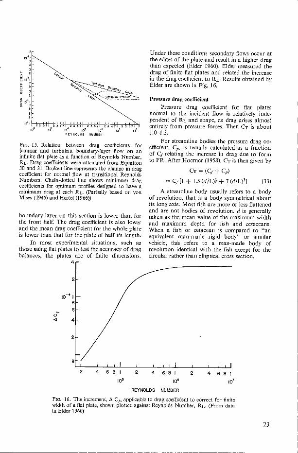
FIG. 15. Relation between drag coefficients for laminar and turbulent boundary-layer flow on an infinite flat plate as a function of Reynolds Number, RL. Drag coefficients were calculated from Equation 30 and 31. Broken line represents the change in drag coefficient for normal flow at transitional Reynolds Numbers. Chain-dotted line shows minimum drag coefficients for optimum profiles designed to have a minimum drag at each RL. (Partially based on von Mises (1945) and Hertel (1966))

boundary layer on this section is lower than for the front half. The drag coefficient is also lower and the mean drag coefficient for the whole plate is lower than that for the plate of half its length.

In most experimental situations, such as those using flat plates to test the accuracy of drag balances, the plates are of finite dimensions.

4 r

Under these conditions secondary flows occur at the edges of the plate and result in a higher drag than expected (Elder 1960). Elder measured the drag of finite flat plates and related the increase in the drag coefficient to RL. Results obtained by Elder are shown in Fig. 16.

Pressure drag coefficient Pressure drag coefficient for flat plates

normal to the incident flow is relatively inde-pendent of RL and shape, as drag arises almost entirely from pressure forces. Then CT is about 1.0-1.3.

For streamline bodies the pressure drag co-efficient, C,„ is usually calculated as a fraction of Cf relating the increase in drag due to form to FR. After Hoerner (1958), CT is then given by

CT = (Cf Cp)

Cf [1 + 1.5 (d/L) - + 7 (d/L) 3 ] (33)

A streamline body usually refers to a body of revolution, that is a body symmetrical about its long axis. Most fish are more or less flattened and are not bodies of revolution. d is generally taken as the mean value of the maximum width and maximum depth for fish and cetaceans. When a fish or cetacean is compared to "an equivalent man-made rigid body" or similar vehicle, this refers to a man-made body of revolution identical with the fish except for the circular rather than elliptical cross section.

FIG. 16. The increment, A Cf applicable to drag coefficient to correct for finite width of a flat plate, shown plotted against Reynolds Number, RL. (From data in Elder 1960)

23

Boundary-Layer Flow Conditionsand Total Drag

Flow conditions in the boundary layer maybe laminar, part laminar-part turbulent (transi-tional), and turbulent, and for each of theseconditions it may be attached or separated.

As the size and speed of a body increase(as RL increases), the boundary layer on a flatplate is first laminar, transitional at RL,r;t, andfinally turbulent, providing the outer flow isstable and the surface is smooth. The boundarylayer on a solid streamline body goes throughthe same phases and, if it is of small width anddepth, the boundary layer will tend to remainattached. However, when width and depth arerelatively large, the pressure gradient downstreanlof the shoulder encourages separation particu-larly as speed and pressure gradients increase.

Interaction of the boundary-layer flow condi-tions and drag components are illustrated inFig. 17 for a streamline body. The lowest dragconditions are obtained only when separationis avoided. Theoretically, only small fish wouldbe expected to avoid separation effects. If it is

Ilaminar partly turbulent laminer partly turbulent

laminar

attached

laminar

separated

FIG. 17. Diagrammatic representation of the relativeeffect of various boundary-layer flow conditions onthe total drag of a streamline body. Shaded areasrepresent frictional drag, DJ, and dotted areas pressuredrag, D. (Front Webb 1970)

assumed they do avoid separation, it is unlikelythey could still achieve the minimum dragconditions found with a laminar boundary layer.This is because the flow in streams, rivers,shoals, etc., is likely to be turbulent. Furthermore,protuberances such as eyes, external flaps on thenares, and fins all behave as large roughnesselements leading to turbulence (Allan 1961).

If the external disturbances are not toolarge, it would still be possible to achieve thetransitional flow conditions. It is probable thatmost fish operate within this range of boundary-layer flow conditions with a laminar boundarylayer to the shoulder, and a turbulent boundarylayer downstream. Exceptions would be manyelasmobranchs with rough skins and possiblylarger cetaceans, which are expected to have fullyturbulent boundary-layer flow.

It is doubtful if many fish actually achieveattached boundary-layer flow beyond the shoulder(see Chapter 4). As such, they experience a muchlarger drag component produced by pressureforces. Figure 17 shows that the advantages ofthe boundary-layer flow conditions are thenreversed as total drag with a turbulent boundarylayer is much lower than with laminar boundary-layer flow. This is because of greater stability ofthe turbulent boundary layer and its greaterresistance to separation which occurs later. Aturbulent boundary layer, at least downstreamof the shoulder, may be beneficial to the reduc-tion of total drag.

It is difficult to reduce the frictional com-ponent of total drag, although minimal drag canbe obtained by specially designed laminar shapesthat extend the favorable pressure gradient up tothe shoulder over as much of the body as possible.It is more advantageous to reduce the pressuredrag component as it is often greater than thefrictional component. A great deal of effort hasbeen expended, particularly by the aircraftindustry, to find mechanisms to reduce pressuredrag. Several successful mechanisms used onaircraft wings and fuselages have been recognizedin fish where they probably serve a similarfunction. These are discussed in detail inChapter 4.

Periodic and Unsteady Motion

Flow patterns described above are applicableonly to bodies moving at uniform velocities. Suchbehavior is not typical of the bodies of many fishwhen at least some portions of the body movewith periodic or unsteady motions. This behaviormarkedly affects flow patterns, although it has

24

generally been assumed that the motion of water around swimming fish will tend toward steady states.

Periodic motion Studies of periodic motions of bodies have

usually been confined to a simple harmonic motion of small amplitude executed by cylinders or plates. When a cylinder moves in this way, normal to its long axis, flow takes on the form depicted in Fig. 18. The periodic motion of the cylinder imparts a steady secondary flow to the whole fluid. This steady motion occurs at some distance from the cylinder and is the result of viscosity of the fluid, although the magnitude of the secondary flow is independent of viscosity. The stable Qecondary flow is only set up after some time and results in a flow toward the cylinder along an axis perpendicular to the motion and away from the cylinder along the axis of the periodic motion.

Unsteady motion The small amplitude periodic motion de-

scribed above is less like that of body movements of a swimming fish, which are of large amplitude. In addition, fish are propelled forward by their body movements so there would probably be

411■■•••■+ FIG. 18. Diagrammatic illustration of the flow around a circular profile moving with simple harmonic motion in the direction shown by double-headed arrow. Broken line shows limit of the boundary layer, and solid lines the streamlines after steady secondary flow has been established. (Redrawn from Boundary-layer Theory by H. Schlichting; © McGraw-Hill Book Co. 1968; used with permission.)

insufficient time to set up steady-state secondary flow. Flow around the body of a fish is probably more similar to that around a body undergoing unsteady motion with periodic stops and starts.

When a cylinder starts to move in a direction normal to its long axis, a boundary layer imme-diately begins to form, increasing in thickness with time and distance moved. Once the cylinder has ceased to accelerate and begins to move at a uniform velocity, the boundary layer rapidly reaches the thickness expected for the relevant Rd. At the same time as the cylinder accelerates, the boundary layer is progressively affected by pressure gradients on the downstream side of the cylinder. Eventually separation occurs, the separation point depending on time (and accelera-tion and final velocity) and distance moved. If the distance moved by the cylinder when separation occurs is Xs, then

X, r 0.351 Rd (34)

and if Is is the time to separation, and U the final velocity

ts 0.351 Rd /U (35)

Bodies and fins used in fish and cetacean propulsion are rarely circular, but elliptical. Values for X. and ts for elliptical bodies depend on dlw, when w is the width in the direction of motion and d is the depth normal to w (Fig. 19). Values for X, for various elliptical shapes are shown as a function of dlw in Fig. 19 which also shows some values for dlw found among fish and cetaceans.

In addition to the boundary-layer phenom-enon, a body starting from rest affects the fluid to some distance from its surface. The effect of the motion spreads through the fluid at the speed of sound (instantaneously for practical purposes) and a relatively large mass of fluid tends to be accelerated with the body. This fluid mass is called the virtual mass or added mass. For the propulsive portions of the bodies of most fish the virtual mass, mv, approximates to

m y p d2 /4 glcm (36)

(Lighthill 1969, 1970).

Similarly, when a body decelerates, the virtual mass will add to the total momentum of the system and must be decelerated with the body. This is particularly important in the case of gliding fish, when a mass of about 0.2 X body mass is generally added to that of the body to calculate the deceleration forces (Gero 1952; Bainbridge 1961).

25

KD - .20

.15

3

caudal 8 peduncles 1 I

.25 caudal fins

.10

.05

1111111 I 1111111

LpP

D

.2 .4 .6 ,8 1.0 2 4 6 8 10 60 100

DEPTH / WIDTH (d/w)

FIG. 19. Relation between distance moved before boundary-layer separation occurs and dimensions of elliptical and circular profiles accelerating from rest. Distance moved before separation (X ) is shown as the ratio of profile width (w), as X,/w. Dimensions of the profile are shown as the ratio of depth (d) to width (w), as dill, . Values for d/w for caudal fins and caudal peduncles of fish and cetaceans are shown, and for caudal peduncle of Bolaenoptera borealis (A) and Enthynnus etas (B). (From data in Hertel (1966) and Magnuson (1970) respectively)

Hydrofoils

Hydrofoil theory has a wide application to the study of fish propulsion, particularly to various aspects of dynamic stability during swimming. The parts of the body which execute propulsive movements have often been compared to hydrofoils to illustrate qualitatively (and sometimes quantitatively) forces acting on the body of a swimming fish. Median and paired fins of many fish behave more obviously as hydrofoils in controlling pitching, rolling, and, to some extent, yawing excursions during swim-ming, and are important in maneuverability. Similarly pectoral fins of scombrids and elasmo-branchs control vertical equillibrium, as do pectoral fins of flying fish.

In all these cases, a surface functions to produce forces perpendicular to the axis of motion and this property will serve as a definition of a hydrofoil. It is, however, usually a require-ment that the perpendicular ("lift") forces be produced with a minimum of drag. Most avail-able information is concerned with aerofoils, but such data can be applied to fish by means of laws of similitude. The term hydrofoil will be used throughout this section as being more appropriate for aquatic vertebrates.

Flow pattern and forces The flow pattern around a flat plate will be

considered as the most simple design for a hydrofoil. When a flat plate of finite width moves along its axis at zero angle of incidence to the flow, the flow pattern can be described by a series of parallel lines (Fig. 20A). The only forces experienced by such a plate will be frictional forces as described above. However, when the plate moves at an angle, the angle of attack, a, to the flow, streamlines are deflected above and below the plate (Fig. 20B). Fluid velocity below the plate is lower than above. Bernoulli's theorem predicts this will be associated with a pressure difference, so that the pressure below the plate exceeds that above. The net pressure difference represents a pressure force, P, acting at some angle to the motion of the plate.

This description of hydrofoil principles is highly simplified. A correct description of hydro-foil function requires consideration of a super-imposed circulation on the purely translational flow. The simplified description is all that is required here; readers interested in greater detail are referred to the monographs listed in the introduction to this chapter.

The net pressure force, P, can be resolved into two components; a lift force, L, acting normal to the axis of motion, and a drag force, D, acting along that axis and retarding the motion (Fig. 20C).

FIG. 20. Flow and forces on a flat plate acting as a hydrofoil: (A) flow around a flat plate at zero angle of attack to the incident flow; (B) flow pattern around a flat plate at a small angle of attack, a, with transla-tional and rotational flow patterns superimposed; (C) forces experienced by hydrofoil in B. Gross pressure force is represented by P, shown resolved into lift, L, and drag, D, components. Boundary layer is not shown. (Redrawn from Theory of Flight by R. von Mises (1945); P Dover Publications Inc.; used with permission)

Flow over the two surfaces of the hydrofoil tends to remain streamlined with boundary-layer separation occurring close to the trailing edge only when a is less than a certain critical value, a„it • Above this value separation of the bound-ary layer occurs close to the leading edge. This has the same effect as early separation on any

A

26

other body. Flow is greatly distorted and an ex-tensive wake is formed (Fig. 21). There is a greatincrease in the pressure difference along the axisof motion, with a concomitant decrease in thatnormal to the axis. Thus, D is greatly increased,and L is reduced. Such a hydrofoil is said to havestalled. At values of a. above stall values, theefficiency of a hydrofoil will be reduced, whichis undesirable, except when hydrofoils are usedas brakes as with paired fins of many fish. Then,the ideal value of U. is 90°.

FIG. 21. Flow pattern around a hydrofoil: (A) belowa_j,; and (B) above when hydrofoil is stalled.(Redrawn from Theory of Flight by R. von Mises(1945); © Dover Publications Inc.; used with per-mission)

GeometryThe geometry of aerofoils is extremely vari-

able and much of this variety is seen in fish. Thus,the plan, profile, and angles subtended to theincident flow and with the body can all vary ac-cording to the requirements of the particular fish.

Basic plans or planforms are shown in Fig.22. Each planform can be characterized by alength or chord, C, and a width or span, S,normal to that axis. The ratio, S/C, is the aspect

AS-

C

B

B

ratio, AR. For arbitrary shapes, as for swept-backand tapered profiles and most fish hydrofoils, ARis calculated from

AR = SIC or SI /Sf, or St, ICI (37)

when St, is the maximum projected area of thehydrofoil. For paired hydrofoils, St, is the totalmaximum projected area for both the hydrofoils,as they usually behave as a single unit.

Fins of fishes, singly or in pairs, are usuallytapered and often swept-back. The same is trueof caudal fins of fish with a well-defined tail.

The plane of paired hydrofoils may berotated relative to the normal plane of the fish. Theangle subtended between the latter horizontalplane and the hydrofoil is the dihedral angle(Fig. 22D). The pectoral fins of Eutlrynnusare so oriented with a positive dihedral angle(Magnuson 1970).

Various types of planform and dihedralangle are related to the stability of the body towhich the hydrofoils are attached. A taperedhydrofoil results in the highest lift forces producedclose to the center of mass, reducing the magni-tude of rolling forces acting on the body in theevent of any asymmetry in the flow. Such plan-forms have obvious structural advantages as theyrequire less heavy support per unit of lifting areathan rectangular hydrofoils of the same area.

Swept-back planforms move the center oflift backward relative to the center of gravity, andaffect pitching equilibrium. This is particularlyimportant in fish when the hydrofoils are often

Fic. 22. Basic types of planforms of hydrofoils: (A) rectangular planform show-ing span, S, and chord, C; (B) tapered planform; (C) sweptback planform; (D)frontal view of a paired hydrofoil showing the dihedral angle, 0. (Redrawn fromTheory of Flight by R. von Mises (1945); © Dover Publications Inc.; used withpermission)

27

mobile. In fish gliding to a halt, continuai variation in the angle of sweepback can often be seen.

The dihedral angle confers stability to yaw-ing, as some component of the pressure force acting on the hydrofoil is oriented laterally. With fixed hydrofoils these forces are balanced, but in fish it is likely that the dihedral angle is varied on either side of the body for fine control during maneuvers.

Variation in hydrofoil profiles in fish is ap-parently less than for man-made aerofoils (Fig. 23). This is because most fins are more like flat plates, operate at lower Reynolds Numbers, and often do not have to produce maximum lift. As a result, the commonest types of profile are similar to those shown in Fig. 23B, D. The first is a simple flat plate, and the second a cambered plate. A cambered hydrofoil has a profile in which the center line is curved relative to a line joining leading and trailing edges. Maximum displacement of this center line, the camber, is usually expressed as a percentage of the chord, the relative camber. Apparently most fins acting as hydrofoils are cambered as in Euthynnus (Magnuson 1970). There are few examples of solid hydrofoils among fish, like those shown in Fig. 23A, C, E. Sections of the pectoral fins of elasmobranchs tend to have some depth (Breder 1926) as do caudal peduncles employed by some scombroid fishes to generate lift (Magnuson 1970). As with relative camber, the maximum thickness, T, characterizing a solid profile, is ex-pressed in relation to the chord length. The ratio, T/C, is called the thickness ratio.

Choice of a particular profile usually depends on the flow conditions under which they operate, as expressed by a Reynolds Number, Rc, based on chord length. For fish, Rc is commonly between 102 to 105 and the highest lift forces and

A T T

D

Fin. 23. Basic profiles of hydrofoils: (A) streamlined, cambered profile showing thickness, T, and camber, c; (B) flat plate; (C) conventional, streamlined profile; (D) cambered plate; (E) streamlined, cambered profile. (Based on Alexander 1968; Hoerner 1958; and von Mises 1945)

the highest lift:drag ratio is obtained with flat plates and cambered plates. Above Rc of about 105 more conventional solid profiles give better results (Alexander 1968).

Equations for lift and drag For a given hydrofoil moving with a uniform

velocity, U, at an angle of attack, a, the lift, FL, and drag, FD, forces are calculated from

FL = p Sh U2 CL (38)

and

FD = p Sh U2 CD (39)

when CL and CD are lift and drag coefficients, respectively. They are often expressed as the lift:drag ratio, as CL/CD or FL /FD. Most hydro-foils are designed for both a maximum CL and lift:drag ratio at the normal operating velocity.

The magnitude of CL and CL /CD depends on the flow conditions, and Rc (see above) on the angle of attack, planform, and profile.

ANGLE OF ATTACK Figure 20C shows that the pressure force

and FL and FD components acting on a hydrofoil will be dependent on a. In practice, CL tends to be linearly related to sine a to a„it (Fig. 24A). Thus

CL = k sine a (40)

when k is a constant for a given hydrofoil. Above acrit, CL decreases markedly with

the disruption in flow over the hydrofoil at the stall.

CD increases exponentially with acrit (Fig. 24B) usually with a minimum value when a is zero. Above acrit, CD increases markedly as CL falls.

The relation between the lift:drag ratio (Fig. 24C) and a increases to a maximum value at a relatively small a because, although CL increases linearly, CD increases exponentially with a.

For values of a above that giving the maximum CL/CD, the lift:drag ratio decreases rapidly, particularly above a crit .

ASPECT RATIO CL is greatest for a hydrofoil of given area

when AR is highest, although in practice, AR values above about 8-10 give little further advantage and are associated with structural problems.

3

28

I I 1 I

0.40

0.35

0-30

0.25

c 0.20

0.15

0.10

0.05

I' 11 I 11 I -0.25 0 -5 0 5 10 15 20 25 30 35 -5 0 5 10 15 20 25

°L 2004. 1— . ° D

5 0 5 10 15 20 25 30

o

1.75

1.50

1.25

1.00

L 0.75

0 • 50

0.25

1.5 •-•••• 0.3

CL/CD

1.0

0.5 —...0.1 441111> Mal

A

▪ CL/CD

20

- 10

NACA 2409

FIG. 24. Relations between CL, CD, and lift: drag ratio with a for NACA 2409 profile. (Redrawn from Theory of Flight by R. von Mises (1945); © Dover Publications Inc.; used with permission)

In contrast, CD is inversely related to AR, as one of the important components of CD is an induced drag component, CI, dependent on AR. This drag component results from the pressure difference between the two surfaces of the hydrofoil which produces cross flows at the hydrofoil tips. The cross flow causes the forma-tion of longitudinal wing tip vortices, the energy dissipated in these being the induced drag. It follows that the greater the AR the smaller the chord length around which cross flow can occur in relation to the total lifting surface. Not only are CI and CD reduced, but a higher mean pressure over the surface is also maintained and CI, is higher. In this respect a tapered planform

can be advantageous in concentrating lift forces away from the wing tips.

PROFILE

The magnitude of CD in particular is affected by any profile differing from a flat plate. This is because a pressure drag component arises in the same way as on a solid body described above. The pressure drag coefficient, Cp, can be approxi-mately related to the thickness ratio (TIC) and to relative camber

Cp = C; + 0.0056 + 0.01(T/C) (41) -I- 0.1(T /C) 2

29

CP is the pressure component dependent onrelative camber: some typical values are inTable 1.

TABLE 1. Relation between relative camber and pres-sure drag coefficient, Cp, for cambered hydrofoil pro-files (from von Mises 1945 .

Pressure dragRelative camber % coefficient (Cn)

U,v, greater than the free-stream incidentvelocity, U.

For a screw propeller to generate thrust,there must be a positive angle of attack betweenthe hydrofoil sections of the blade and theincident flow. This is achieved when the localvelocity of any section exceeds U, the ratiobetween the two velocities being expressed as theadvance ratio, J. Thus, for a section at the tipof a blade

,T = U/co = U/2 n r f (42)

0 0.02 0.00054 0.0016 0.002

A solid profile will also increase the surfacearea of the hydrofoil in comparison with a flatplate of the same chord length and AR. However,the magnitudes of CI and CP are much greaterthan those due to frictional drag, which tend tobe neglected. As hydrofoil lift and drag equationsare usually based on empirical data, the frictionalcomponent is included in practice through itscalculation from such equations as 39.

Center of liftMost problems concerning hydrofoils among

fish are related to stability and maneuverability.As such, it is necessary to know the point at whichthe mean lift force acts to calculate momentsabout the center of mass. The point at whichlift acts, often called the hydrodynamic focus orcenter of lift, can only be found for a givenhydrofoil by experiment. Usually the focus liesbetween 0.25 C (quarter chord point) and0.33 C from the leading edge.

Note on Propellers

Man-made "screw-type" propellers are ob-viously not found in fish. However, the generalprinciples of efficient operation of propellersystems are applicable to the fish propellersystem, and will be briefly considered.

The principles of propeller operation can beunderstood in the light of hydrofoil theory.In a screw propeller each section of a propellerblade moves in a circular path, subtending anangle of attack to the incident flow, the angledepending on the angular velocity of the sectionand the forward speed of the propeller. Move-ments are associated with thrust, the wake formeddownstream of a propeller moving at a velocity,

when

w = angular velocityr = radius of the propeller discf = frequency (revolutions per second).

w varies along the length of a blade so theangle of attack must similarly vary. This accountsfor the "twist" in propeller blades.

For thrust to be generated, J must be lessthan 1. Otherwise, there would be no relativemotion between the water and the blade, anda would be 0.

The same conditions apply to the propulsiveportions of bodies of fish. Gray (1933a, b, c)showed there must be relative motion betweenthe water and moving portions of the body.This condition is realized when the forwardvelocity of the fish, U, is less than the backwardvelocity of the propulsive wave, V. Thus, theratio U/V, comparable in many ways to J,must be less than 1. This ratio was called theslip by Kent et al. (1961).

The mechanical efficiency of a screw pro-peller, i1p, is defined by the ratio between thepower supplied to the propeller shaft, E, andthe thrust power output, ET

rtP = ET/ E (43)

and can be related to J. Similarly, the slip isrelated to the propeller efficiency of the fishpropulsive system, although not as simply(Lighthill 1960, 1969, 1970; Webb 1971b).

As n„ may be related to J, it will also beinversely related to the propeller disc circum-ference from Equation 42 or, more simply,to the propeller disc diameter. Reasons for theadvantage of a large disc diameter are similarto those for high AR. With a large disc diameter,the circumference is small in proportion to thearea across which thrust is generated. Thus, thelarger the disc the relatively smaller the lengtharound which cross flow and energy losses canoccur.

30

•

Furthermore, the larger the disc area the smaller the mass of water that must be accelerated for a given thrust force and the smaller the losses in kinetic energy. This is because the thrust generated is proportional to the mass of the fluid, M, and the increase in velocity given to it. That is

Tp = M (U,, — U) (44)

The kinetic energy, when Tp = thrust KE, required to accelerate the water to the wake velocity is given by

KE = M (11, — U2) (45)

High propeller efficiency can be obtained by increasing the mass of water affected, while decreasing the velocity increase it receives (Alexander 1968).

These principles apply equally to the fish propulsive system. The propeller disc area is equivalent to the product of amplitude of the tail beat and height of the trailing edge of the tail. Bainbridge (1963), Hunter and Zweifel (1971), and Webb (1971a) have shown that the amplitude of the tail beat reaches maximum values as swimming speed increases, presumably because efficiency becomes of greater importance as the limit to the supply of metabolic energy is ap-proached. In addition, the amplitude of the tail beat of several scombrids, among them the fastest aquatic vertebrates, is up to 50% greater than in other fish (Fierstine and Walters 1968).

Equation 44 and 45 show that efficiency can be increased by decreasing the absolute values of 14, and U, as well as their relative values. This is apparently achieved by fish which situate the major portions of the propeller system in the slower wake associated with the drag of the body (Hertel 1966).

Flow Through Pipes

The flow of water through pipes and en-closed pipe systems is important to fish propulsion studies for two reasons. First, fish are often forced to swim inside some enclosed pipe system. Second, the flow through the buccal and opercular chambers and the gill sieve is similar to the flow through an enclosed system of pipes. The resist-ance to the flow through this system contributes to the total drag of a swimming fish.

Flow patterns As with flow around bodies, flow through

a pipe may be laminar, transitional, or turbulent,

depending on the ratio of viscous and inertial forces and other flow conditions discussed above. Different conditions can be compared by Reynolds Law, defining a Reynolds Number, R„ based on the radius of the pipe. The critical value Rr crit is about 103 .

The velocity profile of flow through a pipe depends on the type of flow (Fig. 25). With laminar flow, the profile tends to be curved be-cause of dominant frictional forces. With turbu-lent flow, the flow profile tends to be fairly rectilinear as viscous forces are overridden by the inertial forces associated with the additional motion of fluid particles.

In terms of water tunnel experiments with fish, a laminar flow pattern has an advantage over turbulent flow as it allows normal boundary-layer growth. When flow is turbulent, the intensity of turbulence tends to exceed critical values so that the boundary layer of any body in the flow must also be turbulent. Because of the curved nature of the laminar flow profile, calculation of the mean velocity of a fish within it would be almost impossible. Therefore, a rectilinear profile is desirable, as achieved with microturbulent flow. It was suggested that most fish will swim in a turbulent environment in any case, so the disad-vantages of a turbulent flow are undoubtedly of less importance than the advantages.

A

FIG. 25. Velocity profiles for flow of a fluid with viscosity through circular pipes: (A) laminar flow; (B) turbulent flow.

Law of Continuity and Bernoulli's theorem The Law of Continuity states that flow

through all sections of an enclosed pipe system is constant (technically for thne-independent flow only). If the cross-sectional area of a pipe is Sx and the velocity of flow, U,

Flow = US„ = Constant (46)

In an enclosed system when the cross-sectional area varies, the velocity of flow will also vary in inverse proportion to S. The im-portance of the law comes from its coupling with

31

p U2 R,

2 r

(48)

(49)

Bernouilli's theorem, which predicts that changes in U will be associated with changes in the net fluid pressure. As a result, the pressure in the fluid increases as Sx increases.

These two principles are important in cal-culating the pressure drop associated with gill water flow and can be used in conjunction with the equations given below to calculate gill resist-ance (Brown and Muir 1970).

Pressure drop and resistance to flow The resistance law for the flow of fluids

through pipes is called the Hagen—Poisseuille Law. For laminar flow, the pressure difference

Ap required for a given flow is given by

,Ap = 8 1.12. U/ r2 p U2 (47) — U mean velocity of flow r = radius of pipe

= length of pipe

The last term in Equation 47 represents the kinetic energy of flow. Equation 47 can be rewritten in ternis of RI,

For laminar flow

16. ! Ap =

R: 2

For turbulent flow

0.133 — 4..\/k-r

The flow through the secondary lamellae gill sieve is likely to be laminar, as the dimensions of gills and water flow all combine to make 12, much less than R, era (Hughes 1966; Hills and Hughes 1970). The equations given above are difficult to apply directly to the gill sieve as this tends to be made up of rectangular rather than round spaces. Hughes (1966) calculated an alter-native expression applicable to rectangular tubes

24 / Lp —

5 d3 w q

when d = depth of pores in the sieve w = width of pores q = flow.

p U2

(50)

32

Chapter 2 - Kinematics

Classification of Propulsive Movements

Before discussing various hydrodynamic andbiological aspects of fish locomotion, it isimperative that body and fin movements ofswimming fish be fully understood. Superficialexamination of swimming fish suggests thatthese movements vary markedly in differentgroups of fish. Long thin fish, like eels or blennies,pass a well-defined propulsive wave back overthe body, whereas shorter, thicker fish, like daceor mackerel, appear to swim by moving thecaudal fin alone. Other fish, like the electric fish,Gvmnotus, swim by passing waves along theirmedian fins, while the body remains fairlystraight; others may use paired fins while thebody remains fairly straight; others may usepaired fins as sculls, for example surf perch(Breder 1926; Gray 1968; Webb 1973b).

Breder classified the various movements into

different categories, or modes, after Lighthill(1969). Three main categories are distinguishedon the basis of body and/or fin movements:fish that use their bodies and caudal fins, fishthat use extended median or paired fins, andfish that use shorter median or paired fins. Afourth group of aquatic propulsion mechanismscan be considered for animals using jet propul-sion, the common escape system in cephalopods.Breder (1926) considered this could apply toexhalant respiratory flow in fish, but the volumesof water, and their low velocity (Brown and Muir1970) indicate this would generate negligiblethrust. Jet propulsion is not likely to apply to

fish.

Anguilliform mode: whole body thrown intoa wave with at least one half-wavelengthwithin the length of the body and usuallymore than a complete wavelength. Ampli-tude usually large over whole body length.Body typically long and thin. Named afterthe eel, Anguilla.

Subcarangiform mode: body and caudal finthrown into a wave, with more than onehalf-wavelength within the length of thebody. Amplitude rapidly increases andis large over posterior-half or third ofbody length. Body shape fusiform withdeep caudal peduncle.e.g., Salmo, Carassius, Leuciscus, Gadus.

Carangiform mode: body and caudal finusually thrown into wave, with up to onehalf-wavelength within length of body.Amplitude increasing over posterior thirdof body length, large at trailing edge. Bodyshape fusiform with narrow caudalpeduncle. Named after Caranx.

Carangiform mode with semilunate tail:body movements carangiform. Amplitudeincreasing over caudal peduncle, largecaudal fin. Body shape fusiform withnarrow caudal peduncle and large half-moon shaped caudal fin.e.g. Lamna, Euthynnus, Phocoena, Balaen-optera.

Ostraciform mode: body rigid and notthrown into a wave. Propulsion by meansof caudal fin oscillation. Body shapevariable, but not streamlined. Namedafter family Ostraciidae, e.g., Ostracion.

Fish that use their bodies and/or caudal fins forpropulsion

Most studies on fish propulsion have beenmade on fish that swim by means of body andcaudal fin movements. In this category, Breder(1926) originally distinguished three modes,anguilliform, carangiform, and ostraciform(Fig. 26). Classification of swimming move-ments of fish and cetaceans follows:

Fish that use extended median or pectoral fins forpropulsion

In all cases the fin(s) used are thrown intoa wave formation, similar to the body wave inthe anguilliform mode, but of more constant am-plitude along the fin length (Fig. 26).

Amiiform mode: use extended dorsal fin.Named after Amia.

33

-

AMIIFORM GYMNOTIFORM

Gymnotiform mode: use extended ventral fin. Named after Gymnotus.

Balistiform mode: use extended dorsal ventral fins. Named after Balistes.

Rajiform mode: use extended pectoral fins. Named after Raja.

Fish that use shorted tnedian or pectoral fins for propulsion

In all cases fins pass waves along their length.

Tetraodontiform mode: use short dorsal and ventral fins. Named after family Tetrao-dontidae, e.g., Lagocephalus.

Diodontiform mode: use short pectoral fins with short wavelength movement. Named after family Diodontidae, e.g., Cichlasoma.

Labriform mode: use pectoral fins with long wavelength movement so fins behave as paddles or sculls. Named after family Labridae, e.g., Scams.

Body modes are distinguished based on the number of half-wavelengths of the propulsive wave contained within the length of the body. Thus, in the anguilliform mode at least one half-wavelength is considered to be involved in propulsion, up to one half-wavelength in the carangiform mode, and less than one half-wavelength in the ostraciform mode (Fig. 26).

ANGLIILLIFORM CARANGIFORM OSTRACIFORM

BALISTIFORM

FIG. 26. Some principal types of swimming modes in fish. The portion of body or fins executing lateral movements is shown stippled. (Modified after Breder 1926; Gray 1968)

34

Gray (1968) suggested that the proportion of the body involved in the propulsive wave, and the number of half-wavelengths was dictated by the flexibility of the body.

Many pelagic fish, originally classed as carangiform by Breder (1926), contain more than one half-wavelength within the length of the body, and sometimes more than a complete wavelength (Bainbridge 1963; Fierstine and Walters 1968; Webb 1971a). These fish swim in the anguilliform mode, by definition, although their body shape is more similar to fish swimming in the carangi-form mode. Breder introduced the term sub-carangiform to describe this intermediate type, although he originally restricted the term to more rigid fish like heavily scaled holosteans, e.g., Amiatus. Fish swimming in the subcarangiform mode according to Breder were those which normally swam by means of an alternative propulsion system (i.e. paired fins) but when using their bodies for swimming, tended towards the carangiform mode. The subcarangiform mode used here will refer to all fish that swim in a manner intermediate between the anguilliform and carangiform modes, whether the movements are primary or secondary means of propulsion. The subcarangiform mode includes such families as Salmonidae and Gadidae.

Breder's (1926) original classification con-sidered average types in a continuous range (i.e. true "modes"), and should not be used too rigorously. The addition of further subdivisions, in the light of more complete data, in no way invalidates the original classification, but rather increases its value.

The two main categories of fish that use median and paired fins, are basically similar. The two groups differ in the length of appendages used, so that the only major difference between them is the freedom with which the axis of move-ments can be controlled in relation to the body. This freedom is negligible in amiiform, gymnoti-form, balistiform, and rajiform modes, but high in tetraodontiform, diodontiform, and labriform modes when fin bases are small (Harris 1937).

It is somewhat misleading to attempt to classify modes involving short-based pectoral fins, as fish exercise a high degree of control over these fins, and movements are consequently complex. In Breder's classification, labriform and diodontiform modes are those normally en-countered as the primary locomotory method, whereas other methods usually involving body movements are used in rapid darts, for example

to avoid predators. In addition, paired fin move-ments are common among fish primarily using body movements for swimming. Paired fins may be used for swimming at very low speeds, but otherwise are usually used in stability control (Breder 1926; Harris 1936, 1937, 1938, 1953).

Body and Caudal Fin Movements

Swimming movements involving the body and caudal fin are the most commonly encoun-tered pattern among fish and cetaceans. Fast swimming fish and cetaceans and those making long migrations swim mainly in this way. Seals and manatees have modified bodies and hind limbs that execute swimming movements of similar fashion. Fish that usually use other alternative methods typically resort to body and caudal fin movements for escape maneuvers and fast turns. Most effort has been expended in studying the kinematics of body and caudal fin propulsion, probably because of its ubiquity among aquatic vertebrates.

Anguilliform, carangiform, and ostraciform modes include an extensive range of morpho-logical forms, correlated within each mode. As such, important trends in morphology can be recognized, and it is useful to summarize them. They will be discussed in greater detail in relation to the body forces generating thrust and swim-ming efficiency, in Chapter 5 (Fig. 50). First, the correlation between length and thickness (flex-ibility) with mode has been mentioned. A second trend is the change in distribution of body span (depth) along the length of the fish. In the anguilli-form mode, the span is typically fairly constant along the whole length, and is replaced by a dis-continuous span associated with several median fins (as in gadoids), which in turn is progressively replaced by reduction in number and size of ante-rior median fins with emphasis on the caudal fin. The evolution of a discrete enlarged caudal fin is associated with narrow necking (Lighthill 1969). Narrow necking is the progressive decrease in body span towards the caudal penduncle, with a rapid increase in span over the caudal fin, culminating in the narrow streamline caudal peduncle and semilunate tail of scombroid fish and cetaceans.

The trend to decreasing body flexibility is continued into the ostraciform mode, as these fish are often enclosed within rigid protective cases. This, however, interrupts the trend (seen through the anguilliform and carangiform modes) to more streamlined body shapes and narrow necking.

35

The various body shapes of fish swimmingin different modes should be kept in mind duringthe description of the movements involved.

Anguilliform modeBody movements and principles of anguilli-

form locomotion are basic to almost all otherswimming modes. Therefore, anguilliform kine-matics will be considered first. This has somehistoric precedence, as observations originallymade by Gray (1933a, b, c), particularly on theeel, provided the foundation for most subsequentstudies of fish locomotion. The following dis-cussion is based largely on Gray's observations.

BODY IVIOVEMENTS

As a result of phased muscular contractionson alternate sides of the body, the whole body isthrown laterally into a propulsive wave (Fig.27A). The propulsive wave has a wavelength,XB, with the ratio to length, 7,,B/ L, much less than1. When the fish is swimming forward at uniformvelocity, U, the propulsive wave passes back overthe body at a velocity, V, greater than U. Whenthe fish is decelerating, V may be equal to, orless than, U.

As the propulsive wave passes back over thebody, each small portion of the body, called asegment by Gray (1933a, b, c), executes a periodictransverse motion with posterior segments lag-ging behind immediately anterior segments. Am-plitude of the lateral motion increases withdistance along the body, reaching a maximumamplitude AT toward the trailing edge.

A 7 8u u

b

5 4 3 2

a a a

FIG. 27. (A) body shape during a cycle of propulsivemovements in anguilliform mode, drawn from tracingsfrom photographs (of Anguilla rulgaris) taken at

0.09-s invervals. U = 4 cm/s, V = 6 cm/s. Mean axisof progression is along ab; (B) superimposed outlineof the leading surfaces in A to show the transversefigure eight of a trailing-edge segment. (Redrawn

after Gray (1933a) from Journal of Experimental

Biology Vol. 10)

The locus of each segment in space, relativeto a fixed point in space is a sine curve (Fig. 28)with a wavelength, 7vs less than X. 7,,,s tends to beconstant for all portions of the body, but itsamplitude, A, increases with distance from thenose.

A B C D

mF

5 cm

FIG. 28. Sine curves in space traced by segments alongthe body of Anguilla (A) path of the head; (B) midpointof the body; (C) tip of the tail. The wavelength of thepath, as, is less than the body wavelength, 7,,13, shownin D. Note increase in amplitude of the lateral move-ment of segments along the body. (Redrawn fromGray (1933a) from the Joinnal of ExperimentalBiology Vol. 10)

Following Gray's convention (1933a), thepath of each segment in space subtends anglesOs with the transverse axis of motion, cd, in Fig.27, 28 and following. 0, varies periodically withthe transverse motion of a segment. Mean valuesof Os decrease as the amplitude increases withdistance from the nose (Fig. 31).

The locus of a segment in space, relative toa point moving along the axis of progression, ab,

and at velocity U (that is relative to the fish) is atransverse figure eight. This is most clearly seenfor a segment at the trailing edge (Fig. 27B). Thetransverse figure eight is a result of the propulsivewave passing backward over an inextensible body.Because of the figure eight motion, rather thana simple linear transverse motion, segments donot execute pure simple harmonic motion.

The transverse motion of each segmentresults in fluctuating transverse velocities andaccelerations. The change in transverse velocity,W, and acceleration, a, for a hypothetical seg-ment moving symmetrically about ab and cd can

36

VE

LO

CIT

Y

AC

CE

LE

RA

TIO

POSITION TIME

be related to the position of the segment in space and time (Fig. 29). In space, W is zero at positions of maximum displacement, + A/ 2, accelerating to reach its highest value, \Yr.., as the segment crosses the axis of progression. W tends to be fairly constant at Wmax for about 0.5 A, half the distance covered by the transverse motion. In terms of time, Wmax represents about 0.2 of the time, t, for a cycle.

For acceleration, changes in a to amax to a occur over about 0.5 A. In terms of time, these changes represent about 0.8 t.

U and W are the components of the motion of a segment most easily measured, but the veloc-ity of a segment relative to the water is the resultant of these. The resultant velocity, WR, may be calculated from a triangle of velocities, when at some instant

wR -Vwz + u2

The value of O s is given by the same triangle as

Tan Os = U/W (52)

Theoretically, the value of U for a given segment varies during a cycle of transverse move-ment because the figure eight motion has velocity components along the axis of motion. How-ever, variations in U will be negligible in com-parison with U and W and may be neglected.

For uniform forward motion, changes in a along the axis of motion depend only on the figure eight motion. As with U, variations in a along this axis will be negligible in relation to transverse changes in a, and may be neglected.

The magnitudes of a and W are obviously dependent on A, and will increase with distance from the nose (leading edge).

Superimposed on the transverse motions of each segment is a rotational component, out of (51)

z o I- CI) o a_

+A i

0

—A .F TIME

FIG. 29. Relation between the transverse velocity and acceleration of a hypo-thetical segment in relation to position and time. Motion of the segment in space is between limits of + A/2, each cycle taking a time, t, as shown at top. Further explanation is given in the text.

37

phase with the transverse motion by 70-900 (Hertel 1966). Continuing to follow Gray's

(1933a) convention for angles, each segment sub-tends angles OB with the transverse axis of motion. This angle varies with position (Fig. 30), ap-proaching 90° at + A /2, and a minimum value as the segment crosses the axis of progression. The magnitude of OB depends on the amplitude of the motion as does Os, and is higher for more anterior segments in the same way (Fig. 31).

FIG. 30. Diagrammatic representation of the figure eight motion of a segment relative to the fish, with rotational motion superimposed. This is shown by the changing angle subtended by the segment relative to the axis of transverse motion, cd, during half the cycle. Successive positions are numbered. (Redrawn from Gray (1968) with permission of Weidenfeld and Nicolson Ltd.)

The relation between the angles subtended by the path of a segment and the rotational corn-ponent define the angle at which the incident water with velocity WR strikes a segment. For uniform forward motion, OB is greater than 0,, as 1B is greater than 4. The difference between the two angles is the angle of attack, a, which is then

134 B — (53)

The angle, a, is important as it indicates the amount of lateral motion of the body relative to the water. When a segment is compared with a hydrofoil (e.g., Taylor 1952) it can be seen that forward thrust can only be generated when a is positive, although this analogy only strictly applies to steady flow.

RELATIONS BETWEEN BODY MOVEMENTS

Because of the increase in amplitude of the lateral motion of segments with distance along the body, the value of a and WR will also vary with a segment's position along the body. The interrelations between a and WR with position can be illustrated for a hypothetical fish swim-ming in the anguilliform mode. The limits of + A/2 in relation to the axis of progression can

be shown by two curved lines (Fig. 3IA), and, to simplify the discussion, the amplitude at the nose will be assumed zero. Within the limits of the motion of the body, enclosed by the lines showing + A/ 2, the figure eight motion of four segments along the body can be shown. Instantaneous values of W, with U constant, can be used with triangles of velocity to calculate instantaneous values of WR and Os, as shown for the instant when each segment crosses the axis of progression in Fig. 31B. The rotational component of motion of the segments can be superimposed on such diagrams with the relevant instantaneous value of OB, to obtain a.

From vector diagrams for all positions and values of W throughout a cycle, changes in a and WR can be shown for each segment (Fig. 31C). a and WR are inversely related with the position of the segment, so that a is higher for anterior seg-ments, whereas WR is higher for posterior seg-ments. Gray (I 933a) interpreted the effectiveness of the propulsive wave in terms of the change in momentum given to the water after being de-flected by a segment through the angle a. The correlations between a and WR imply a balanced distribution of thrust-per-unit-mass of water affected along the body. Because of the increasing area of influence of the propulsive wave with increasing amplitude, more water will be affected by the propulsive wave travelling down the body associated with progressively increasing velocities, WR. The propulsive wave can be considered as increasing the total mass and momentum of water in the system, reaching a maximum at the trailing edge. By the use of hydromechanical models, Lighthill (1966, 1970) has shown that the thrust generated by a fish is mainly given by the amount of momentum shed into the wake at the trailing edge.

The hypothetical fish discussed represents the most simple case of symmetrical movements and uniform forward velocity. It can be seen from Fig. 31C that under these conditions a is highest when WR is highest, that is, when a segment crosses the axis of progression. Nursall (1958b) observed that a may be minimal when WR is highest. This is presumably the result of active control by the fish over the propulsive wave, probably to smooth out thrust fluctuations in response to instantaneous requirements. A similar interpretation has been made by Bainbridge (1963) to explain the complexities of the behavior of the caudal fin of fish swimming in the subcarangiform mode.

38

a

06

06

WR

FIG. 31. Relations between the angle of attack, a, subtended between a segmentand the incident resultant velocity of the water, WR, for segments at variouspositions along the body of a hypothetical fish swimming at velocity U. (A)position of segments along the body for figure eight transverse motion, betweenthe limits ± A/2, increasing with distance of segment from the nose. Angle Onsubtended between the segment and the axis cd, is illustrated as the segmentcrosses the axis of progression ab, moving from - A/2 to + A/2; (B) vectordiagrams relating the velocities W, U, and WR with 0B as the segments cross ab.0s is the angle subtended between WR and cd, and a is given by OB-0s; (C)relation between a and WR calculated from vector diagrams for the motion ofsegments during a half cycle.

KINEMATIC REQUIREMENTS FOR GENERATION

OF THRUST

Kinematic requirements for generation ofthrust have been mentioned briefly. Movementsof the body must result in lateral motion of asegment relative to the incident water flow, thatis, a must be positive. This requires that OB and?.B must exceed 0,s with ).,•, which occurs when Vexceeds U. For a given propulsive wave, as Uincreases toward V, a decreases as the wave-lengths of the body and path of a segment ap-proach each other. When U equals V, the path ofa segment coincides with the shape of the pro-pulsive wave along the body. Then there is norelative motion between the body and the water,other than tangential motion. In real situations,the tangential motions associated with frictionaldrag would result in deceleration of the fish untila new equilibrium was reached for a new relationbetween V and U, when thrust equalled drag.

It is also possible for V to be less than U.Then the propulsive wave will generate negative

B C

thrust, or drag, in the opposite direction to theforward motion of the fish. The propulsive wavecould, therefore, be used as an active brakingsystem. As far as it is known, no observations ofthis form of motion have been made, possiblybecause it would be more costly energeticallythan braking by use of paired fins. It should alsobe noted that many fish can swim backwards(Hertel 1966; Gosline 1971).

Carangiform modesCarangiform modes include fish with fusi-

form bodies, swimming in a range from what istechnically the anguilliform mode to the spe-cialized carangiform mode with a semilunate tail(see p. 42). According to Lighthill (1969, 1970)and Wu (1971b, c) the hydromechanical theorydescribing the anguilliform mode is applicableto similar movements, classed as subcarangiformand carangiform modes, up to some stage whenthrust is generated exclusively by the caudal fin.This is reached in fish that approach or include

39

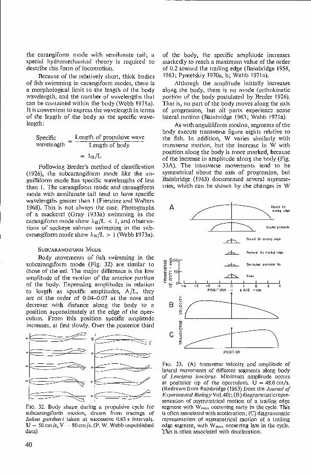
the carangiform mode with semilunate tail; a special hydromechanical theory is required to describe this form of locomotion.

Because of the relatively short, thick bodies of fish swimming in carangiform modes, there is a morphological limit to the length of the body wavelength, and the number of wavelengths that can be contained within the body (Webb 1971a). It is convenient to express the wavelength in terms of the length of the body as the specific wave-length:

Specific Length of propulsive wave wavelength — Length of body

= kB/L

Following Breder's method of classification (1926), the subcarangiform mode like the an-guilliform mode has specific wavelengths of less than 1. The carangiform mode and carangiform mode with semilunate tail tend to have specific wavelengths greater than 1 (Fierstine and Walters 1968). This is not always the case. Photographs of a mackerel (Gray 1933a) swimming in the carangiform mode show 113 /L < I, and observa-tions of sockeye sahnon swimming in the sub-carangiform mode show XB /L > 1 (Webb 1973a).

of the body, the specific amplitude increases markedly to reach a maximum value of the order of 0.2 toward the trailing edge (Bainbridge 1958, 1963; Pyatetskiy 1970a, b; Webb 1971a).

Although the amplitude initially increases along the body, there is no mode (orthokinetic portion of the body postulated by Breder 1926). That is, no part of the body moves along the axis of progression, but all parts experience some lateral motion (Bainbridge 1963; Webb 1971a).

As with anguilliform motion, segments of the body execute transverse figure eights relative to the fish. In addition, W varies similarly with transverse motion, but the increase in W with position along the body is more marked, because of the increase in amplitude along the body (Fig. 33A). The transverse movements tend to be symmetrical about the axis of progression, but Bainbridge (1963) documented several asymme-tries, which can be shown by the changes in W

A

Caudal peduncle

Caudal fin

Dorsal fin trailing edge

Pectoral fin trailing edge

Operculum posterior tip

SUBCARANGIFORM MODE Body movements of fish swimming in the

subcarangiform mode (Fig. 32) are similar to those of the eel. The major difference is the low amplitude of the motion of the anterior portion of the body. Expressing amplitudes in relation to length as specific amplitudes, A /L, they are of the order of 0.04-0.07 at the nose and decrease with distance along the body to a position approximately at the edge of the oper-culum. From this position specific amplitude increases, at first slowly. Over the posterior third

Fio. 32. Body shape during a propulsive cycle for subcarangiform motion, drawn from tracings of Salina gairdneri taken at successive 0.03 s intervals. U = 50 cm /s, V = 80 cm /s. (P. W. Webb unpublished data)

'Lî 100 — U)

IL

▪

I

›- 50 - z o ▪ o

▪ I>j -4 -3

None

-2 -I 0 I 2 POSITION - 4/2 -cri

Il 3 4

POSITION

Flo. 33. (A) transverse velocity and amplitude of lateral movements of different segments along body of Lenciscus lenciscus. Minimum amplitude occurs at posterior tip of the operculurn. U = 48.0 cm/s. (Redrawn from Bainbridge (1963) from the Journal of Experimental Biology Vol. 40); (B) diagrammatic repre-sentation of asymmetrical motion of a trailing edge segment with W1110> occurring early in the cycle. This is often associated with acceleration; (C) diagrammatic representation of asymmetrical motion of a trailing edge segment, with Willa x occurring late in the cycle. This is often associated with deceleration.

40

during a cycle. Bainbridge (1963) found that for dace, goldfish, and bream the distribution in W was sometimes shifted so that W max occurred early in a cycle (Fig. 33B). In one case the opposite was found, with Wrnax occurring late in a cycle (Fig. 33C). These asymmetries were often associated with accelerations and decelerations, respectively.

In fish swimming in the anguilliform mode, the propulsive wave tends to be transmitted along the whole length of the body by muscular forces. In carangiform modes, the caudal fin is interposed between the body and the trailing edge, and the propulsive wave must be transmitted over a relatively passive portion of the body (Gray 1933c). The caudal fin is extremely flexible in fish swimming in the subcarangiform mode. Under the influence of both hydrodynamic and body muscular forces, coupled with a small amount of intrinsic muscle, the caudal fin has a complex motion of its own. This is shown by anterioposterior bending, dorsoventral bending, and variations in the span of the trailing edge during a cycle (Bainbridge 1963) as indicated in Fig. 34.

The degree of freedom in anterioposterior bending is given by the fin rays. These form

FIG. 34. Diagrammatic representation of caudal fin bending when swimming in subcarangiform mode. For the time shown, the propulsive wave overtakes the tail and motion of anterior and posterior edges is shown by arrows. A rigid tail would take the shape shown by the chain dotted line. Trailing-edge span is shown as S, and dorsoventral bending is measured relative to this, as h.

a girder system of half-rays, each half-ray is free to move relative to the other, up to a limit. This limit defines the maximum anterioposte-rior bending (McCutcheon 1970). Up to this limit, anterioposterior bending depends almost entirely on hydrodynamic forces (Gray 1933a; Bainbridge 1963). According to McCutcheon (1970) the shape of the tail is defined by these forces and the behavior of the fin rays is such that the shape of the tail ensures a suitable distribution of thrust over its surface. Thus, the shape varies in relation to the instantaneous changes in load that occur during a cycle. McCutcheon (1970) described this behavior as selfcambering.

In contrast to bending along the anterio-posterior axis, bending in the dorsoventral plane appears to be only partly because of hydro-dynamic forces, although they are still of greatest importance. Curvature of the fin increases as the tail moves away from positions of maximum am-plitude, tending to reach a maximum at the end of a transverse cycle. The more flexible fin center then continues to move in the same direction although the return stroke commences with the stiffer portion of the fin moving in the opposite direction. At this point, the curvature of the fin is minimal, but the fin is wrinkled. The degree of dorsoventral bending is not in phase with the transverse motion of the tail (Bainbridge 1963), as shown in Fig. 35, but can largely be attributed to the expected behavior of water on the flexible center of the fin.

If dorsoventral bending was the result of hydrodynamic forces only, then a direct correla-tion would be expected between changes in span and curvature. This is because the curvature would represent the "bellying" of the fin center between the limits set by the stiffer outer fin rays. Bainbridge (1963) found that span and curvature were not well correlated and were subject to extensive variation (Fig. 35). Bainbridge thought the fish exercised some active control over behavior of the fin, by means of the intrinsic fin muscles observed in several fish (Greene and Greene 1914). Observations of independent movements by individual sections of caudal fins of several fish indicate the activity of an intrinsic caudal fin muscle system (Breder 1926; von Holste and Kuchemann 1942; Harris 1937; Bainbridge 1963; Webb 1971a).

The net effect of dorsoventral bending and changes in span is a rhythmic variation in the projected area of the caudal fin. Variation in the caudal fin area of the fish studied by Bainbridge (1963) was of the order of 10% of the mean area.

41

1_ 47C

0.8

PHASE

+A/2r

o L o I -A/2

1 1 1 1 1 1 1 0 71 271 371

PHASE- ad

02 0.4 0.6 TIME - s

FIG. 35. Relations between caudal fin trailing-edge motion, trailing-edge span, and dorsoventral bending in Leuciscus leuciscus. Movements of the trailing edge in space are shown for rc/2 divisions of a cycle by dots on the traces of span and bending. Note the poor correlation between various motions and movement of the tail. (Redrawn from Bainbridge (1963) from the Journal of Experimental Biology Vol. 40)

As with span and bending, the area changes were poorly correlated with other kinematic factors, but generally, area was lowest at positions of maximum displacement ( + A/ 2), increased rapidly as the tail accelerated away from these positions, and tended to reach maximum area at Wmax. This maximum area was usually main-tained for the remainder of the cycle.

In addition to these rhythmic changes in caudal fin behavior, P. W. Webb (unpublished data) found that depth increased with speed for rainbow trout swimming up to 2 body lengths/s. Depth apparently reaches and remains at maxi-mum values approaching this speed and above. Maximum depth would involve maximum masses of water in propulsive movements and increase thrust and efficiency at these speeds when available energy expenditures would begin to limit further higher performance.

In view of the active control by fish over much of the movement of the caudal fin, it is probable that variations in area during a cycle express control by the fish over thrust produced in response to instantaneous requirements. Other more rhythmic changes were interpreted by Bainbridge (1963 p. 48) in terms of: "a) to allow a

rapid initial acceleration of the tail by virtue of its smaller area; b) to maintain a high and uni-form thrust when the transverse speed of move-ment is falling by increasing the area of the tail at that time; c) to facilitate slowing of the tail by this increased area; d) to add a minimum of drag to the moving body by presenting a minimum area to the water when at the extreme lateral positions in the cycle of movement." Although the complex caudal fin movements can be ration-alized, it is difficult to measure instantaneous thrust. Consequently, effects of bending and span variations have not been quantitatively measured.

THE CARANGIFORM MODE

Apart from the photographs published for mackerel by Gray (1933a), no observations have been made on fish swimming in this mode. Body movements are intermediate between the sub-carangiform and carangiform mode with semi-lunate tail. Otherwise, it is probable that detailed kinematics, particularly in relation to fine tail movements, would be simpler than in the sub-carangiform mode and closer to the carangiform mode with lunate tail. This is because the caudal fins of fish swimming in the carangiform mode tend to be scooped out, so that the fin lias a swept-back planform (Nursall 1958a; Lighthill 1969). As a result, fin rays become more closely aligned with the span, making the fin stiffer and reducing dorsoventral bending. In addition, the length of the caudal fin becomes smaller, and anterioposterior bending is represented only in the rotational component of motion like that of a body segment in the anguilliform mode. Rotational motion of the tail differs from that of a segment, as it can be more closely controlled by body and caudal fin musculature (Fierstine and Walters 1968).

THE CARANGIFORM MODE WITH SEMILIJNATE TAIL

The carangiform mode with distinctive semilunate caudal fin lias evolved independently in four separate groups of aquatic vertebrates, apparently for two different reasons. Most aquatic animals that swim in this mode are those swimming at high speeds with high efficiency (Lighthill 1969). This includes Lamnid sharks from the elasmobranchs, percomorph fishes from the teleosts, and cetacean mammals. The char-acteristic body shape is also found in the extinct aquatic reptile Ichillyosaurus (Wallace and Srb 1961; Lighthill 1969), so that it, too, probably swam in the carangiform mode with semilunate tail.

E-- E3

3§.

42

The second use of this type of propulsion isapparently associated with slow swimming (Bone1971). Bone observed two swimming patterns in adeep-sea trichiurid fish, Aphanopus carbo: (1) fastswimming in the anguilliform mode using theerected long dorsal fin and body; (2) slow swim-ming in the carangiform mode using a highlyswept-back caudal fin, and the median fin furled.Aphanopus probably stalks its prey, detecting itby means of the lateralis system. Effective usageof the lateralis system requires a long stablebaseline and minimal local pressure fluctuations.This is achieved by holding the body straight as incarangiform swimming, with anguilliform pro-pulsion used within striking distance of the prey(Bone 1971). Q. Bone (personal communication)considered that such usage of two swimmingmodes may be a common occurrence, and applyto such fish as Lophotes (see Fig. 50). Gymnarchusalso approaches this carangiform mode, pre-sumably to keep the body straight for efficientelectrical reception.

Except for dolphins and porpoises, propul-sive movements are apparently the same in thevarious groups that swim in the carangi form modewith semilunate tail (Fig. 36). Significant lateralpropulsive movements are confined to the caudalpeduncle and caudal fin. The form of propulsivewave differs somewhat from that of other fishthat swim by means of body movements, in thatthe wave tends to be transmitted across a double-joint system (Parry 1949a, b; Nursall 1956;Slijper 1958; Kramer 1960; Fierstine and Walters1968; Pershin 1970). The first major axis of bend-ing is the anterior base of the caudal peduncle;motion around this axis results in lateral dis-placements of the tail. The second major axisis the base of the caudal fin. This permits therotational motion required to ensure a positiveangle of attack. The motion of the caudal fin issimilar to that of a segment of the body at thetrailing edge in subcarangiform motion. Becauseof the double joint system, the wavelength is

Fic. 36. Body shape during a propulsive cycle inEuthynnus affinis swimming in carangiform mode withsemilunate tail. Figure drawn from successive photo-graphs taken at 0.06s intervals. U = 8.2 L/s.(Modified after Fierstine and Walters 1968)

long and the specific wavelength tends to bebetween I and 2.

Compared to the specific amplitudes oflateral movements in the subcarangiform mode,those of the carangiform mode with semilunatetail are lower anteriorly, but can reach highermaximum values posteriorly. In Eut/rynnus affinisA /L is of the order of 0.03 at the leading edge and0.3 at the trailing edge (Fierstine and Walters1968). Typically, A/L is of the order of 0.21 atthe trailing edge (Hunter and Zweifel 1971).

Measurements of W and a for E. finis haveshown asymmetrical caudal fin movementssimilar to those occasionally found by Bainbridge(1963) in goldfish. Wmax tended to occur towardthe end of a cycle, after the tail had crossed theaxis of progression, resulting in a more uniformand longer acceleration phase for the caudal fin(Fierstine and Walters 1968). These authors alsofound that a tended to be maximum early in thecycle, with lower W, and lowest toward the endof a cycle, with W highest. The inverse relationbetween W and a, is analogous to that of seg-ments along the body in anguilliform motion,and was interpreted by Fierstine and Waltersas a mechanism for smoothing the developmentof thrust.

As with the carangiform mode, the caudalfin skeleton (fin rays) tends to be oriented alongthe span of the caudal fin, so that its own motionis relatively simple. There is still some dorso-ventral bending, but in the opposite sections ofthe fin to that observed in the subcarangiformmode. In Euthynnus, the center of the fin leadsand the tips follow, because the center of the finis more rigidly attached to the body than the tips.This contrasts with the subcarangiform modewhen dorsal and ventral fin rays are stiffer andconsequently more rigidly attached to the bodythan those at the center. The magnitude of bend-ing of the semilunate tail is much less than that ofthe caudal fin in the subcarangiform mode(Fierstine and Walters 1968).

The kinematics of cetacean locomotion aregenerally similar to those of fish swimming in thecarangiform mode with semilunate tail (Fig. 37)except movements are in the vertical plane (Gray1968). Dolphins and porpoises differ somewhatfrom the general picture, as the body is oftenthrown into a sharp curve (Slijper 1958, 1961;Lang and Daybell 1963; Pershin 1970). The tailstroke also tends to be asymmetrical in time andspace. For example, the stroke tends to bemostly below the axis of the body, rather thansymmetrical about that axis (Purves 1963). In

43

6 5 4 3 2

FIG. 37. Body shape during a propulsive cycle of Lagenorhynchus obliquidens, to show carangiform motion with semilunate tail in a porpoise. Drawn from photographs taken at 0.2 s intervals. U := 348 cm/s. (Modified after Lang and Daybell 1963)

addition, the upstroke may be shorter, with higher W, than the downstroke. Usually rotation of the tail maintains a favorable relation between W and a (Parry 1949a, b; Lang and Daybell 1963), although in sonie cases there is division into an active and a recovery phase in each cycle (Purves 1963).

RELATIONS BETWEEN SWIMMING SPEED AND KINEMATICS

For certain species of fish swimming in carangiform modes, quantitative relations have been established between U and the kinematics of the propulsive wave represented by f and A or AIL. This approach was pioneered by Bainbridge (1958) for dace, goldfish, and trout swimming in the subcarangiform mode. Bainbridge con-cluded that: (1) the distance covered per tail-beat was proportional to A for a given fish; (2) for a given A, U was linearly related to f for a given fish, but this relation did not pass through the origin; (3) for a given f and A, the specific swimming speed, U/L, was the same for fish of different lengths for the three species studied.

These relations have generally been con-firmed for fish swimming in the subcarangiform mode (Smit et al. 1971; Webb 1971a) and for several fish swimming in other carangiform modes (Magnuson and Prescott 1966; Yuen 1966; Pyatetskiy 1970a; Hunter and Zweifel 1971).

For fish swimming in the subcarangiform mode, the original equations relating U/ L and f found by Bainbridge (1958) appear to apply for swimming speeds greater than about 1 to 2 L/s. Relations between A and the distance moved are only important at speeds lower than these, as then both A and f vary with swimming speed, and U/L is linearly related to the product f A/ L

(Webb 1971a, 1973a). A increases as frequency and speed increase to reach a maximum of the order of 0.2 L (Hertel 1966; Hunter and Zweifel 1971). Thus, the linear relation between U/ L and f, with AIL fairly constant, includes A/ L in the slope (Table 2).

For other carangiform modes, it appears there is less variation in A and f at low speeds, so the whole speed range can be expressed as a function off only (Hunter and Zweifel 1971).

The various constants found for different species of fish for U/L = af + 1) or U/L pro-portional to afA/L are included in Table 2. Complete equations for U/L vs f AIL have not been given. Most measurements were made at high swimming speeds whereas f and A appear to be important only at low speeds. Few meas-urements have been made in the latter speed range. The slope, a, in the equations varies two-fold for the range of species studied, showing that some fish obtain higher specific speeds (in L /s) at a given tail-beat frequency than others. Table 2 shows there is no particular correlation between the value of a and swimming mode. Lowest values are found for Sardinops swimming in the carangiform mode, and Thunnus and Euthynnus swimming in the carangiform mode with semilunate tail. The highest value was found for Triakis, a shark that probably swims fairly close to the anguilliform mode (Hunter and Zweifel 1971). Most values tend to cluster around 0.74-0.83.

Values off and A do not completely charac-terize the propulsive wave in terms of thrust, so it is not valid to draw too rigorous conclusions based on the slopes for different species. For example, a general interpretation would suggest that those species with low a would tend to be less efficient than those with high a values. Low a, associated with high f at a given U/L, implies the water is accelerated to a greater extent in relation to the incident water velocity than with high a. The greater the acceleration given to the water, the greater the kinetic energy losses, implying that several fish swimming in the car-angiform mode with semilunate tail might be relatively inefficient. Although there is no sup-porting experimental evidence, this is contrary to general biological opinion based on swimming performance and the predictions of hydro-dynamic models.

The most probable reason for the apparent discrepancy relates to other kinematic factors. The various relations between U/ L and f are for given species, and the relation will apply to a

44

Length Mode (cm)

U/L a

Speed range U/L = af b • afAIL (Lis) a b A /L a Species Reference

0.75 -1.00 0.18 4.10 Bainbridge (1958)

2-15

1-3.5 0.82 -2.6 0.20e 3.20

0-3 0.74 -1.8 0.19 3.91

0-10 0.93 -0.49 0.21 4.43

CSL

13.6

30b

I5b

0-10

0-10

0-10

Hunter and Zweifel (1971)

2.38

3.90

3.95

TABLE 2. Relations between swimming speed (U/L) and propulsion kinematics as A/L and f for fish swimming in carangiform modes. Keys: SC, subcarangiform mode; C, carangiform mode; CSL, carangiform mode with semilunate tail.

Leuciscus leuciscus SC 5.2-24.0

Salmo(irideus) SC 4.0-29.3 gairdneri

Carassius SC 4.6-22.5 auratus

Carassius SC 15 auratus

Salmo gairdnerl SC 28.2

Triakis henlet SC 23.6

Mugi! cephalus SC 26.5-30.0

Pomatomus saltatrix C 42

Smit et al. (1971)

Webb (1971a)

Hunter and Zweifel (1971)

0.5-6 0.82 -0.72 0.20a 3.60 Pyatetskiy (1970a)

Sarda (=Pelamys) CSL 13.8-16.3 sarcla

Sarda chiliensis 45-59 0-6.5 0.64 +0.49 0.20e 3.20 Magnuson and Prescott (1966)

Sardinops sagas

Scomber japonicus

Trachurus symmetricus

Thunnus albacares

Euthynnus pelamis

CSL 51.9 0.5-14.4

CSL 57.2 0.5-14.4

0.50 +0.21 0.21

0.82 -0.72 0.21

0.83 -1.02 0.21

0.57 +2.45 0.20a 2.84 Yuen (1966)

0.50 +2.05 0.20a 2.50

aAssumed specific amplitude. bKinematic parameters measured for large size range, and high dependence of those parameters with length.

Values shown for center of length range rested.

given form of propulsive wave dictated by mor-phological considerations. The form of the propulsive wave varies between modes, and in the carangiform mode with semilunate tail in parti-cular, the double joint system will permit high control of such kinematic factors as a. This

degree of control is probably far greater than that possible for fish swimming in modes between sub-carangiform and carangiform, because of the rela-tively passive nature with which the shape of the fin varies with load (McCutcheon 1970). Accord-ing to prediction based on hydromechanical

45

models (Lighthill 1970), the magnitude ofa as well as other kinematic factors will affectpropulsive efficiency (and the magnitude ofthe thrust). It is likely that swimming efficiencyof fish that swim in the carangiform modewith semilunate tail with low values of a ismarkedly affected by greater active control overa than would be expected for more "typical"propulsive waves.

None of the equations relating U with f passthrough the origin, and detailed relations forfish of different lengths are not identical. In mostcases, the bias introduced by length-dependentfactors is small, with the exception of some fishswimming in the carangiform mode with semi-lunate tail (Hunter and Zweifel 1971). Moreaccurate, unbiased estimates of the relationbetween U and f have been elaborated by Hunterand Zweifel, and these take the form

U - Uo = a[L( f- fo)] (54)

when U. and fo are the speeds and frequencieswhen the general relation between U and f crossthe appropriate axis for a fish of a given size.Establishing a model of this type obviouslyrequires much more effort than for those given inTable 2, but Hunter and Zweifel ( 1971) consideredthat the unbiased models could be useful in thefield for identification of fish in sonar studies.

Ostraciform modeAs far as is known body and caudal fin

movements of fish swimming in the ostraciformmode have not been described in detail (Gray1968). Bodies of such fish are usually enclosed ina rigid nonstreamlined integument, and the tailarticulates with the body at a well-defined jointat the base of the fin. The tail tends to be fairlyrigid. Ostraciform locomotion does, however,lend itself to the construction of mechanical andhydrodynamic models, because of the relativesimplicity of the morphological system. In me-chanical models described by Breder (1926), Smithand Stone (1961), and Gray (1968), the tail wasrepresented by an oscillating rigid plate. Theauthors found that such models generated signif-icant propulsive forces, with positive componentsthroughout the cycle.

The tail probably has some flexibility, inwhich case the observations made by Gray(1933c) on a whiting with the caudal fin amputatedmay be applicable to the ostraciform mode inthe absence of observations on the mode itself.In the whiting, the tail movements were asym-metrical in space and time in relation to the fish

(Fig. 38). The motion comprised an initial highacceleration from positions of ± A/2, followedby a fairly uniform phase of constant velocity atW,,,aX occupying about three-quarters of thetransverse movenlent and a similar portion of thetime for one cycle. The cycle was terminated bya short deceleration phase. a tended to be positiveduring most of a cycle, but became negativeduring the deceleration phase. During the periodof fairly constant velocity at Wmax, the tail barelymoved forward in relation to the environment,whereas the head moved forward both in relationto the tail and the environment, shown by thebody straightening in relation to the tail. Thuswith the tail pushing against the water, the fishmoved forward because its body resistance wasmuch lower than the tail portion. These move-ments are similar to initial phases of acceleration(Weihs 1973a) but of smaller amplitude.

Fia. 38. Body shape during a propulsive cycle for

Gadus merlmrgus after amputation of tail. This isprobably similar to motion in the ostraciform mode.(Redrawn from Gray (1933c) from the Journal of

Experimental Biology Vol. 10)

46

It should be remembered that ostraciformpropulsion is not a primary locomotor method(Breder 1926). Fish swimming in this mode haveprotective mechanisms other than speed, andare often found in situations where free move-ment is restricted. The primary locomotor methodtends to be paired or median fin movementswhich permit slow, but highly maneuverablemovements. The tail serves as a rudder duringslow swimming and is otherwise used for highspeed acceleration.

Median and Paired Fin Propulsion

Median and paired fins of fish and cetaceansare most commonly used to control stability.Sharks, teleost fish swimming in the carangiformmode with semilunate tail, and cetaceans pri-marily use their fins in this way. Powered finlocomotion is, consequently, less ubiquitous thanbody and caudal fin modes, and generally foundin association with the anguilliform, subcarangi-form, carangiform, and ostraciform variations.Some skates and rays use pectoral fin propulsionexclusively. Otherwise, fin propulsion is employedfor low speed, usually high maneuverable loco-motion, supplemented or replaced by body andcaudal fin propulsion for high speed swimmingand fast turns (Breder 1926; Harris 1936, 1937,1938, 1953; Nursall 1962; Webb 1973b).

Few studies of fin propulsion have beenmade, the majority confined to teleosts (Breder1926; Harris 1937, 1953; Breder and Edgerton1942; Lissman 1961; Nursall 1962; Webb 1973b)with some superficial observations on rays(Breder 1926). Generally, a propulsive waveis propagated anterioposteriorly for forwardmotion. When pectoral fins are oriented dorso-ventrally, waves pass in this direction as it is theembryological anterioposterior axis (Harris 1937).

Major variations in fin kinematics can berelated to the length of the fin and number ofwavelengths within that length similar to theclassification of body and caudal fin modes.The long fins in amiiform, gymnotiform, balisti-form, and rajiform modes contain severalhalf-wavelengths within the fin length - similarto anguilliform propulsion. Diodontiform andtetraodontiform modes involve short fins generallywith less than one wavelength, similar to sub-carangiform or carangiform propulsion, whereasthe short, often relatively stiff, fins in the labri-form mode frequently behave in a similar fashionto ostraciform propulsion.

Specific wavelengths, calculated relative tothe length of the fin base, range from much lessthan I for the dorsal fin of Hippocampus, amii-form mode (Breder and Edgerton 1942); andventral fin of Gymnarchus, amiiform mode(Lissman 1961); through 1.3 for the pectoral finsof Balistes, diodontiform mode; to 5.3 for thepectoral fin of Epinephales, labriform mode(Harris 1937).

Other differences between the kinematics ofmajor fin and body modes are large. Specificamplitudes (relative to length of fin base) are ofthe same order as body modes for long fins,between 0.16 and 0.24 in Hippocampus (Brederand Edgerton 1942). However, there is no increasein specific amplitude along the length of the fin.In pectoral fin modes, the maximum amplitudeis found at the fin leading-edge tip (Harris1937). In Cymatogaster, labriform mode, specificamplitudes reach maximum values of approxi-mately 10 (Webb 1973b).

When fins have a long base and relativelylow specific amplitudes, maximum frequenciesof lateral movements appear to be higher thanfor body modes. Breder and Edgerton (1942)reported maximum frequencies of 70/s in Hippo-campus. When amplitudes are higher, as in themovements of short-based pectoral fins, fre-quencies are lower and of the same order ascaudal fin beat frequencies at similar speeds.Thus, the pectoral fin of Cymatogaster beats atfrequencies of 4/s at a 45-min critical swimmingspeed of 3.9 L/s (Webb 1973b).

Detailed movements of other fins are far morecomplex than those of the body or caudal fins.Propulsive waves can be passed in either directionwith facility. Individual segments are capable offairly extensive independent movement becausemuscular forces are transmitted to stiff fin rayssupporting a thin, highly flexible finweb. Althoughfin rays are restrained proximally when theyarticulate with the body, distal portions can moveanterioposteriorly to some extent as well aslaterally. Variations in wavelength, amplitude,and, to a lesser extent frequency, can occurwithin the length of the same fin at the same time(Breder and Edgerton 1942).

Short-based pectoral fins are capable of adifferent form of variation because the axis of thefin motion can be rotated on the fin base. Whenpectoral fin movements are made about a dorso-ventrally oriented fin base, rotation of the finmotion permits thrust to be generated posteriorly,laterally, or anteriorly. However, this motionrequires an action and recovery phase in eachstroke to maintain motion in a given direction.

47

Propulsive forces can be generated throughout a pectoral fin beat cycle by rotating ventral seg-ments relative to dorsal segments, so that the fin moves at an angle, or by passing propagated waves along the fin (Harris 1937, 1953).

More common in fish than rotation of the axis of motion of various fin segments is to couple this with rotation of the fin base. For example, the fin base of Cymatogaster subtends an angle of about 35° to the long axis of the body, so the fin surface always subtends some angle to the incident flow. During abduction positive thrust and vertical forces are generated, and during adduction a similar thrust force and nega-tive vertical force are generated (Webb 1973b).

When fish using pectoral fin propulsion are forced to swim in a current, regular swimming patterns are adopted in some preferred mode, and the magnitude of variation in movements is reduced. In Cymatogaster, swimming speeds between 0.5 and 2 L/ s are associated with shorter wavelength pectoral fin movements replaced by more "scull-like" (long wavelength) move-ments between 2 and 4 L/s. Each type of motion can be characterized in terms of frequency and amplitude of the fin beat, so the product is linearly related to swimming speed (Fig. 39). Pectoral fin movements are supplemented by caudal fin movements between 3 and 4 Lis in Cymatogaster. Caudal fin propulsion replaces pectoral fin propulsion at about 1 L/s in Lepomis (Brett and Sutherland 1965).

Concluding Comments

When propulsion movements are considered in terms of the motion of individual segments, there is a marked similarity among most modes. Variations among modes can largely be attributed to the number of segments involved in the pro-pulsive wave and the closeness of their coupling.

SPECIFIC SW 3 IMMING SPEE0 — L/s

FIG. 39. Relation between the product of pectoral fin beat frequency (/second) and amplitude (radian) with specific swimming speed in Cymatogaster aggre-gala. Arrow indicates speed at which the kinematics changed from labriform propulsion with long wave-length propulsive waves passed along the fins to a more scull-like beat. (Modified after Webb 1973b)

In body modes, segments are closely coupled within the inextensible framework of the body. They are capable of large amplitude lateral move-ments within the propagated wave. Fin segments of long fins are capable of relatively small amplitude movements because they are con-strained proximally by the body, but otherwise coupling is loose. The inability of long fins to achieve high amplitudes may be the reason such fin motions are associated with low swimming speeds. Higher swimming speeds are attained with fin motions of higher amplitude which only appears to be achieved by pectoral fin modes.

It seems probable that a general reduction in the number of segments involved in locomotory movements is associated with increases in pro-pulsive efficiency (see Chapter 5).

4

48

( , SUSTAINED (CRUISING) ACTIVITY

TRANSITION

PROLONGED (STEADY) ACTIVITY

Oncarhynchus nerka

TRANSITION

BURST (SPRINT)

ACTIVITY F

Solma gairdnerl

3 4 5 6 7 8

SWIMMING SPEED — L/s

10-2

0 1 2 9 10 II 12

103

102

0

I

-

10

Chapter 3 — Swimming Speeds

Introduction

Having considered the kinematics of pro-pulsion, levels and magnitudes of swimming per-formance achieved by fish that swim in various modes may be discussed. Of all facets of ver-tebrate aquatic locomotion, swimming speeds have been most exhaustively studied. In common with many other aspects of locomotion, these studies have been largely confined to a few groups, mainly animals swimming in carangiforna modes.

In view of the magnitude of data on swim-ming speed, it is not possible, nor desirable, to present a detailed discussion; an excellent review has been published by Blaxter (1969). Instead, various activity levels will be defined as used subsequently in the present work, and orders of magnitude of swimming speeds at these levels will be indicated.

Swimming Levels

Three main swimming activity levels have commonly been distinguished on the basis of the time for which a given speed can be maintained: (1) cruising or sustained, (2) prolonged or steady, (3) sprint or burst levels. Each principal level can be identified from a speed-duration curve (fatigue curve) that shows a wide range of speed and dura-tion. After appropriate transformation of data (often with log time plotted against speed) such a fatigue curve may be resolved into three straight lines corresponding to the principal activity levels (Fig. 40). Between each level is a short transition zone.

These levels are based on locomotion in a primary locomotor mode involving body and caudal fin propulsion. As such, the three levels commonly identified are considered insufficient to adequately describe the diversity of fish activi-ties. It is suggested that the three main categories should be designated principal locomotor levels, subdivided as appropriate to provide a more flexible descriptive framework for fish locomotor behavior. The terms to be used are as follows:

Sustained (Activity level maintained for longer than 200 min.)

Routine. Low levels of routine activity, e.g.,

FIG , 40. Fatigue curves for sockeye salmon, Omar-hynchus nerka, and rainbow trout, Salmo gairdneri, showing three principal activity levels. Broken lines indicate transition zones where variability is expected to be greatest. (Modified after Brett 1964, 1967b)

foraging, station holding, by individual fish or loose schools, exploratory movements, territorial behavior. Schooling. Low levels of routine activity of fish or cetaceans in organized schools. In-cludes similar activities to routine activity but also migrations. Cruising. Higher levels of steady swimming activity, including preferred speeds of nega-tively buoyant fish, etc.

Prolonged (Activity level maintained between 200 min and 15 s.) Subdivisions possibly based on physiological criteria (Pritchard et al. 1971).

Burst (High activity levels maintained for less than 15 s.)

Sprint. High steady swimming speeds. Acceleration. High unsteady swimming activity.

Sustained levels As a principal activity level, sustained swim-

ming speeds have been critically discussed by

49

several authors, particularly Brett (1964, 1965a, b,1967a). Brett (1967a) recommended standardprocedures for measuring activity at sustainedlevels in experimental situations, and these recom-mendations may serve as a definition. Sustainedswimming would include all speeds and /or loco-motor activities maintained for a minimum of200 min. This definition includes a wide range oflocomotor patterns assigned to three groups:routine, schooling, and cruising.

ROUTINE

Routine activity includes all low level activ-ities normally seen in free-swiminingfish, whetherin primary, secondary, or both, locomotor modes.Routine activity levels will be the mechanical andbehavioral equivalents to routine metabolic levelsas defined by physiologists (Brett 1972).

SCHOOLING

This activity level includes many character-istics of routine activity except that the activityinvolves organized groups of fish. Schoolingactivity frequently includes migration. For someschooling species there is probably a hydro-mechanical advantage to members of the schoolthat permits more energetically economicalswimming performance (Belyayev and Zuyev1969; Zuyev and Belyayev 1970; Weihs 1973b).

CRUISING

Cruising activity is identified by highersteady swimming speeds than are typical ofroutine activity, and, in most cases, by schooling.This description embodies the unstated definitionof sustained activity in the literature where suchlevels are based on experimental techniques whenfish are forced to adopt a specified relatively highactivity level sustained for fairly long periods.

In wider terms cruising will again overlapwith other activity levels, in this case with school-ing activity in migrations. Preferred swimmingspeeds of fish that are negatively buoyant andmust swim continuously to control vertical sta-bility are included. Preferred speeds are probablyminimum speeds for the most efficient generationof required lift forces (Magnuson and Prescott1966; Magnuson 1970).

Prolonged levels

Prolonged activity levels are defined in rela-tion to sustained activity, and burst activity asspeeds that can be maintained for between 15 sand 200 min. Prolonged activity is frequentlyassociated with periods of cruising with occa-sional bursts.

Most experimental observations on swim-ming fish have been made for prolonged activity.An important concept in such studies is the ac-curate measurement of the critical swimmingspeed, U,,;, (Brett 1964). The measurement ofUc,•;t stems from the convenient increasing veloc-ity test procedure whereby various mechanical orphysiological parameters may be measured for arange of speeds up to exhaustion of the fish. Insuch a test, swimming speed is increased bydiscrete intervals AU every t min. If a fish is ex-hausted in t; min following a speed incrementfrom U to U + AU, then

Ucrit - U + (55)

and Ucr;t is qualified as the t-min U,r;t.Some controversy exists over the requisite

value for t. Brett (1964, 1965a, 1967a) recom-mended 60 min when data for oxygen consump-tion are required. AU and t must consequentlybe large. Alternatively, Dahlberg et al. (1968)considered t may be as small as 10 min whenU,,-;t alone is required, with DU being cor-respondingly smaller.

The U,;t results probably tend fairly closeto sprint speeds for the 10-min time increment(Fig. 40), whereas the longer 60-min period isknown to be about 12% higher than maximumcruising speeds (Brett 1964).

Any speed increment is followed by someperiod of restlessness by the fish (Webb 1971a, b)and some time is required for the cardiovascularand ventilatory systems to adjust to the changeddemands of the tissues (Stevens and Randall1967a). The latter adjustments take place overapproximately 5 min, similar to the maximumperiod of restlessness observed by Webb. Inview of the time required to adjust to a higherspeed, any t value of less than about 20 minmay be too short. Otherwise the adjustmentperiod occupies a substantial period of time spentat any speed.

In an increasing velocity test AU is constant.The power required to swim at any speed isproportional to Uz•s. It would be expected thatthe magnitude of required physiological adjust-ment for successive speed increments wouldbecome progressively larger as such a testproceeded, with a possible reduction in theperformance of a fish. Preliminary experimentswith sockeye salmon in an increasing velocity testwith equal (Ut2•s - Uz•s) increments gave similarU,;t values to identical tests with equal AUincrements (P. W. Webb unpublished data)but the question should be pursued further.

50

Burst

SPRINTS

Sprint activity includes high steady swimming speeds maintained for less than approximately 15 s. This generalization apparently applies to a wide variety of fish (Blaxter 1969).

The definition includes speeds maintained for less than 1 s, but it is likely these should not be considered as steady speeds but as unsteady peak speeds attained following an acceleration burst.

ACCELERATION Acceleration activity may be defined as a

high level of unsteady activity, probably main-tained for less than 1 s. Such phenomena have largely been neglected in research, although acceleration is an integral part of a predator—prey relation and obviously the high sprint speeds attributed to fish can only be reached after an initial acceleration.

From the few measurements made for fish of a wide size range, typical acceleration values appear to be of the order of 40-50 m /s2, in-dependent of size (Gero 1952; Gray 1953a; Hertel 1966; Fierstine and Walters 1968; Weihs 1973a).

Included in this level of activity should also be high speed maneuvers, which have mechanical similarities with acceleration (Weihs 1972, 1973a).

There may be some overlap between accel-eration at both burst and sustained activity levels. Normal routine activity will include some bursts interposed by glides. Such activity was considered the common form of routine activity among fish, called by Houssay (1912) "nage filée." Weihs (1973d, 1974) has shown that fish swimming at routine levels in such a burst / glide fashion can achieve significant energy savings. The magnitude of accelerations in routine activity may be such that there is no real overlap with burst acceleration activity.

Intermediate levels Between each principal activity level is a

transitional zone, characterized by extensive variance in swimming behavior as fish elect primarily one or another adjacent principal level. Prolonged activity may be interpreted as an intermediate level. Hunter (1971) and Pritchard et al. (1971), for example, have shown that inter-mediate swimming may be subdivided for Trachurus, the subdivisions related to the type of fuel oxidized and the site of usage.

Swimming Speeds and Size Effects

A useful concept in fish and cetacean locomotion studies is expressing swimming speeds in relation to length. Speeds may be expressed as specific swimming speeds in body lengths/ s (L/ s) after Bainbridge (1958). This normalization method is useful in comparing performance of fish of different sizes under various conditions, although it has recently been shown that size effects can be more accurately defined than in terms of Us alone (Dahlberg et al. 1968; Hunter and Zweifel 1971). Specific swimming speeds remain the simplest and most useful method of comparison and will be used in the absence of detailed data on performance-size effects for most fish and cetaceans.

Most measurements of swimming speed have been made for fish swimming in various body and caudal fin modes, as with most other aspects of locomotion (Blaxter 1969). Even from these measurements it is clear that few interspecific generalizations can be made (Beamish 1966); the frequently accepted "10 L/ s rule of thumb" for maximum sprint performance should cer-tainly be treated with caution. In any propulsion study, it is imperative that performance levels should be determined for the pertinent experi-mental conditions. For present purposes it is sufficient to summarize briefly the magnitudes of various swimming performance levels reported for fish of different sizes, considered in terms of swimming mode whenever possible.

Anguilliform mode

Few measurements of swimming speed have been reported for fish swimming in this mode. Blaxter (1969) quoted sprint values of 3 L /s for a 10 cm Piles and 1.9 L /s for a 60 cm Anguilla (Fig. 41). A size effect on sprint performance is suggested, but clearly the data are insufficient to attempt further conclusions. Pleuronectids also swim in the anguilliform mode, at least at higher performance levels (Breder 1926; Stickney and White 1973), although the body is markedly com-pressed in comparison with more typical fish swimming in this mode. These fish achieve slightly greater sprint speeds, apparently independent of size up to about 35 cm (Fig. 41).

Subcarangiform and carangiform modes

Pooled data taken from the review by Blaxter (1969) for sprint speeds are plotted against length in Fig. 41. ln all groups of fish when speeds have been measured for a large enough size range,

51

13

Clupeoids

( Cyprinids and Perclds

tCorossius

12

I I

I0 Le)

_1 , 9

w 8

Salmonids

Gadlds

6 2

CI) 5

C-)

w 0 4 [ o_

Pleuronectids \ u... . _

7

y Clupeoid Percids

Anguilla

(i) 3 e

e Pholls

30 40 50 60 70 80 90 100

LENGTH — cm FIG . 41. Relation between maximum specific speeds and length for several groups of fish. Solid lines show maximum sprint levels, broken line highest cruising levels reported for fish. (Data taken from Brett (1964), Brett and Glass (1973), and Blaxter (1969) who may be referred to for further references)

•I0 20

there is a marked dependence of specific speed on size, specific speed decreasing with increasing size. This is particularly well shown for gadids, e.g., Cactus morhua (Blaxter and Dickson 1959). For several groups, specific speeds appear almost independent of length to approximately 30 cm, but this is only a superficial result of pooling data.

Measurements on a given species show size dependence (Blaxter 1969; Beamish 1966).

The relation between specific sprint speeds and length for smaller clupeiods is of particular interest. The initial rapid increase in specific speed in young fish occurs with the elaboration of the caudal fin. Increased depth of the caudal

52

fin produces more efficient propulsion, to whichthe rapid increase in specific speed might berelated. The increase in specific speed to a peakfollowing caudal fin elaboration is followed bya marked size-dependent decrease in specificsprint speed comparable to that observed forgadids (Fig. 41).

The best generalization Blaxter (1969) couldreach concerning sprint speeds of fish of differentgroups, was that small salmonids, cyprinids, andpercids could achieve maximum sprint speedsof the order 9-12 L/s, not dissimilar to the 10 L/sspeed considered typical of fish by Bainbridge(1958), on the basis of earlier literature andhis observations on a relatively small size rangeof three species. Blaxter (1969) considered thatmost other fish, including clupeoids and gadids,could normally reach maximum sprint speedsof 4-9 L/s.

In comparison with sprint speeds, cruisingand prolonged speeds show much greater vari-ance, not only between species but also to agreater extent as a result of biotic factors (Brett1962). Figure 41 shows for completion the orderof magnitude of maximum cruising speedsmeasured for salmonids, clupeoids, and percidsunder optimum conditions (Brett 1965a; Blaxter1969; Brett and Glass 1973). Other groups canapparently reach cruising speeds of the order ofhalf to three-quarters of these values (Blaxter1969).

Carangiform mode with semilunate tailThis mode of locomotion is employed by

fish and cetaceans reaching the highest swimmingspeeds, not only in terms of absolute speeds, butin terms of specific swimming speeds. Fishswimming in this mode have commanded sub-stantial research interest probably because of themagnitude of speeds recorded. Because manyreach large sizes, the animals are not usuallysuitable for rigorous experimental observation,with the exception of experiments conducted byHunter and Zweifel (1971). Most swimmingspeeds have consequently been measured on largefish and cetaceans swimming in large aquaria(Magnuson and Prescott 1966; Yuen 1966), bytiming from boats over some distance (Parry1949a; Johanessen and Harder 1960; Yuen 1966),or by allowing a fish to run out a line (Gero 1952;Walters and Fierstine 1964). In many cases,speeds may be uncertain, particularly if the animal

cannot be seen at all times, and the method ofrunning out a line has obvious disadvantages asdiscussed by Gero (1952). Additional reliable

data on performance levels and their maxima arerequired for larger fish and cetaceans.

The various groups of fish and cetaceans willbe considered separately.

SCOMBRIDS

Swimming speeds at various activity levelsare shown in Fig. 42. Maximum specific sprintspeeds to 21 L/s have been reported for Tiunnus

albacares (Walters and Fierstine 1964). Thesespeeds were only maintained for a fraction of asecond and were peak unsteady speeds reachedafter a period of acceleration. Nevertheless, max-imum sprint speeds of 10 L/s and above appearto be the rule for scombrids, including those oflarge size. Little dependence of speed on size hasbeen found, except for Euthynnus pelamis (Fig.42). Schooling speeds have been reported forscombrids between 0.5 and 10 L/s and cruisingspeeds were reported of the same order (Blaxter1969; Hunter and Zweifel 1971).

ELASMOBRANCHS

Few data have been reported for elasmo-branchs swimming in carangiform modes. Gero(1952) measured what were probably sprintspeeds for Carcharhinus leucas 153 cm long, and

22

20

18

EulAynnus

4-

6

4

2

° 50

'EUlhynnus

1 bTh-us

60 70 eo 90

LENGTH - cm

A-mo rei m3 J

100 110

Fic. 42. Relation between specific swimming speedsand length for scombrids. Solid circles and spacewithin quadrilaterals are maximum sprint speeds, opencircles are schooling speeds. (Data shown for Euthyn-nus pelamis, Acanthocybiam solanderi, Yuen 1966;Sarda chiliensis, Magnuson and Prescott 1966; andThunnus albacares, Walters and Fierstine 1964,Yuen 1966)

53

o

r‘ureoPs .ePseudorco *Mc

alege

1/4 6Yobiocepholo

Eschrichtius

Baloenopterat:

5

1

w 4 LJ a.

2 3

2 ;,49/717nousco & s wick

11111111111111 0

["-Phocoena 6

..

Delphinus

41 Phocoenoldes

I'1/4•Lagenorhynchus

1Globlocepholo

Orcinus

Negaprion brevirostius 184 cm long, of between 3.4 to 3.9 L/s. These speeds are low in comparison with other animals swimming in the same mode and many swimming in other modes. Clearly more data are required.

CETACEANS Swimming speeds of cetaceans are sum-

marized in Fig. 43. A few of the largest cetaceans attain slightly higher sprint speeds than scom-broid fish, dolphins, or porpoises (Gawn 1948), but in general there is little increase in swimming speed for a size range from approximately 100 to 3600 cm. There is a marked dependence of specific swimming speeds on size, and maximum recorded specific swimming speeds are extremely low for large cetaceans. Maximum specific sprint speeds for Ba/aenoptera appear to be of the order 0.5-6.3 Lis (Gray 1936b; Gawn 1948; Norris and Prescott 1961).

2 3 4 5 6 7 8 9 36 37 LENGTH - cm x10-2

FIG. 43. Relation between specific swimming speeds and length for cetaceans. Solid circles are maximum sprint speeds; solid squares and shaded quadrilaterals, cruising speeds; open circles and stippled quadri-laterals, schooling speeds. (Data shown for Phocoena conununis, Gray 1936b; Delphinus delphus and D. bairdi, Gray 1936b, Norris and Prescott 1961; Phocoenoides dalli, Tursiops gilil, Eschrichtius glaucus, and Pseudorca crassidens, Norris and Prescott 1961; Globiocephala melana, G. scanunoni, and Lagenorhyn-chus obliquidens, Johanessen and Harder 1960, Norris and Prescott 1961; Balaenoptera borealis, Gawn 1948; and Orcinus orca, Norris and Prescott 1961)

Specific cruising swimming speeds also show marked size dependence from 4.4 to 2.1 Lis for a length of 215-760 cm. For Balaenoptera 3672 cm long, sustained speeds fall as low as 0.3 Lis. Schooling speeds range from 2.2 to 0.4 Lis, again showing size dependence (Fig. 43).

Summary — For animals swimming in the carang-iform mode with semilunate tail maximum sustained speeds approach maximum burst speeds fairly closely. In general, scombrids cruise be-tween 5 and 10 Lis, with sprint speeds of the order 1 0-1 6 L/s. For cetaceans, these values are 2-5 Lis and 3-7 Lis respectively. In comparison, an intermediate-size salmon would cruise at approximately 3 Lis with sprints up to approxi-mately 9.5 Lis, a much greater difference, particularly as propulsive power required in-creases with U 2 .8 . Animals swimming in the carangiform mode, with the semilunate tail modification are apparently designed for high speed sustained activity levels.

Other swimming modes Measurements at various activity levels have

not been made for fish swimming in other modes, with the exception of prolonged swimming for Cymatogaster aggregata (Webb 1973b). A 45-min Umt of 3.9 L/s was found for fish 14.3 cm long swimming in the labriform mode. This value compares favorably with many optimum pro-longed swimming speeds of other fish swimming in body and caudal fin modes.

Factors Affecting Swimming Speeds

Swimming speeds are affected by numerous factors depending to a large extent on the activity level. This applies particularly to sus-tained and prolonged activity levels, which have been most extensively studied. Sustained and prolonged activities are dependent on the main-tained functioning of supply systems for oxygen and removal of waste metabolic products. Any factor interrupting or affecting supply systems, as well as those affecting the propulsive system itself, affects swimming performance. Burst activity is dependent on immediate energy reserves and appears to be less affected by extraneous factors (Blaxter 1969).

Factors that affect sustained swimming performance will be summarized for completion. More detailed reviews may be found in Brett (1962) and Blaxter (1969) or any standard comparative physiology text.

54

GOVERNING - T LIM.TING - 0, A6Ir

4e

■Zi, 5 ,0 -

INITIAL

1 I I 10 16 20

TEMPERATURE - C

1.0 , 25

TEMPERATURE

This is probably of greatest importance. Although it apparently has little effect on sprint performance (Blaxter 1969) temperature markedly affects sustained swimming. An exception is Clupea harengus (Blaxter 1969). The response to temperature depends on the temperature to which fish are acclimated and the test temperature. When these are the same, a peaked curve is typical (Fig. 44). A more domed shape appears when acclimation temperatures are constant, and fish are then tested at different temperatures. In terms of overall energetics, at critical swim-ming speeds, the metabolic cost to travel unit distance appears to be independent of tem-perature (Brett 1964).

FIG. 44. Relation between swimming speed of sockeye salmon acclimated to 15 C only and tested at various temperatures, and acclimated to each test temperature. (From Brett 1964) Mean lengths were 16.8 and 17.8 cm for the two groups respectively. Effect of environmental factors, temperature (T) and oxygen (02) on activity are indicated in the manner of Fry (1947). (From Brett I967a)

OXYGEN AND CARBON DIOXIDE

Reduction of oxygen between 90 and 60% air saturation reduces performance in salmonids. For fish acclimated to lower levels, oxygen

levels of 60% saturation are required before per-formance is affected (Dahlberg et al. 1968). High oxygen levels above air saturation can increase performance (Brett 1964). At high temperatures, the oxygen content of water is reduced, and this reduces performance, over-riding temperature effects that would be expected to increase performance (Brett 1964). High levels of carbon dioxide apparently have little effect on performance (Dahlberg et al. 1968).

SALINITY Salinities that differ from normal levels

reduce performance, although the reduction is small compared to temperature effects (Blaxter 1969; Griffiths and Alderdice 1972).

PREEXERCISE Training has mixed effects on performance.

In general, training results in higher swim-ming speeds (Brett et al. 1958; Vincent 1960; Bainbridge 1962; Blaxter 1969).

PREHISTORY Hatchery-reared fish usually have lower

swimming speeds than wild fish (Davies et al. 1963). This may be the result of less training in hatchery fish (Hammond and Hickman 1966). In addition, the conditions under which eggs are hatched, in salmonids at least, affect later swimming performance (Barns 1967). There are also performance differences between stocks (Brett 1964).

HANDLING Handling is a stress resulting in elevated

metabolic rates, probably related to oxygen debt. Recovery from handling may take up to 8 h (Black 1957) or more (Smit 1965). Insufficient recovery times are expected to result in reduced prolonged and burst speeds through reduction of immediate reserves and elevation of catabolite levels.

MATURITY Fish approaching sexual maturity tend to be

less excitable and have reduced performance (Blaxter 1969).

Chapter 4 - Drag

Introduction

Drag is the resistance to motion of a bodymoving in a fluid. The question of the drag ofswimming fish is of fundamental importance topropulsion studies, particularly in consideringthe energy flow through the "black box" that isthe composite propulsion system. Only whenoxygen consumption can be related to swimmingspeed is there any comprehensive information onenergy input to this system, but the overall anddetailed fate of that energy is largely unknown.Initial characterization of the propulsion systemrequires information on efficiency, which in turnis contingent on calculation of power expend-iture against drag.

There are two approaches to calculatingpower expenditure; by calculating drag force, orthrust force that must be equal to the drag of thefish.

Measurement of thrust is more difficult thandrag (Webb 1971a) and the use of this approachlargely depends on the formulation of suitablehydrodynamic models consistent with the kine-matics. Until recently, no suitable models wereavailable, and these could not be tested againstmeasurements. The only criteria available forthe acceptance of a model was that its predictionsshould not violate the laws of thermodynamics,and be consistent with the expected behavior ofthe system interpolated from measurements onother animals.

Because of difficulties in calculating thrust,biologists and mathematicians have tended tocalculate swimming power requirements fromdrag. Two methods have been used. Both assumeflow around a swimming fish is mechanicallyequal to flow around an equivalent rigid body(rigid-body analogy). Then drag may be calculatedfrom standard hydrodynamic equations, i.e. theo-retical drag. Alternatively drag may be measuredfor a (usually dead) fish with the body stretchedstraight, i.e. dead drag. The use of the rigid-bodyanalogy in calculating drag for swimming fishappears to be based on observations first madeby Sir George Cayley (1809, see Gibbs-Smith1962) that fish and cetaceans with high swimmingperformance all have streamlined bodies.

The application of drag calculations toenergetic studies has produced confusion, asconclusions are conflicting. The most importantstudy was made by Gray (1936b), who calculatedthere was insufficient muscular power to meetthat required to overcome the theoretical dragfor a dolphin. This has since been called Gray'sparadox, and has stimulated much research torepeat or explain the discrepancy. Similar dis-crepancies have been found on the basis oftheoretical drag for salmon by Osborne (1961),goldfish by Smit et al. (1971), and on the basisof dead-drag measurements by Brett (1963). (SeeChapter 7.)

In contrast, Bainbridge (1961) calculatedthat almost all fish and cetaceans could developsufficient muscular power to meet their theo-retical drag power requirements. Similar resultswere attained by Smit (1965) for goldfish and byBrown and Muir (1970) for skipjack tuna. Webb(1970) and A. J. Mearns et al. (personal com-munication) reached similar conclusions fromdead-drag measurement of salmon and trout.

Much of the confusion can be attributed toinsufficient information on other components ofthe propulsive system or swimming performancelevels. Some discrepancies can be resolved in thelight of more complete later data. Nevertheless,it is important to reconsider the question of dragmeasurements and their application to fish powerproblems.

Theoretical Drag

Theoretical drag is the hydrodynamic resist-ance of an equivalent rigid body, with the samedimensions as the fish to which it is compared,moving at the same velocity in the same fluid. Inextrapolating theoretical drag calculations toswimming fish, it is implied that swimming dragis equal to that of the body when stretchedstraight and making no lateral movements. Assuch, the flow pattern is assumed to be streamline,with boundary-layer flow conditions dictated byRL, surface conditions, and the intensity of tur-bulence. The effects of any secondary flow patternproduced by propulsive movements are neglected.For practical purposes, most calculations of

57

theoretical drag assume the fish is not compressed, and may be compared with a body of revolution, the diameter of which is the mean of the depth and width of the fish. Otherwise, the shape of the body is assumed to be similar to that of the fish in ternis of its effects on flow (Chapter 1).

Drag arises from skin frictional forces and longitudinal pressure forces acting on the body, fins, and gills. Drag from gills has been neglected except for calculations made by Brown and Muir (1970) for the skipjack tuna (Katsmvonis pelamis) and these will be considered. The fish was 44 cm long, and calculations were made for the pre-ferred swimming speed of 66 cm/s, taken from Magnuson (1970). Other values required for calculation of drag are given in Table 3. RL was 3 X 105 , below RL cm, so the boundary layer was assumed to be laminar.

For the body, the pressure drag coefficient, Cp , was taken as 0.25 the frictional drag coeffi-cient (Cf For the fins, Cp of 0.5 Cf was taken. This higher value was used because tuna are denser than seawater and lift is generated by the pectoral fins (Magnuson 1970). The value of C,, used was the mean for lifting and nonlifting fins. The total drag for body and fins was calculated as 10,930 dyn.

Gill resistance was calculated using the principles of flow through pipes and engineering experience of energy losses in expansion and contraction sections. Bernoulli's theorem and the laws of the conservation of mass and momentum were used to calculate pressure changes in the expansion section of the system (the buccal cavity), and the contraction section (the opercular cavity). Pressure losses in the two sections were estimated to be 15% of the pressure change in the buccal cavity, and 5% of the pressure change in the opercular cavity. Pressure change across the gills was calculated from Poisseuille's law for the flow through pipes of the measured dimensions of the gill sieve.

Total pressure loss across the gill system was calculated as 1100 dyn/ cm2, which represented a total drag of 1090 dyn.

From these data, the drag of body and me-dian fins was 77% of the total drag, and that of the pectoral fins 14% (Table 3). This suggests that use of the paired fins as hydrofoils is an expensive method of buoyancy control; the relatively high drag of the pectoral fins was associated with only 3% of the total body and fin area. The gills represented 9% of the total drag (although their area was 30 times that of the

body and fins) because the water velocity over the secondary lamellar surface was low, as required for efficient gas exchange (Muir and Kendall 1968; Randall 1970a, b).

Other studies using theoretical drag calcula-tions have been made for dolphins (Gray 1936b), salmon (Osborne 1961), goldfish (Smit 1965; Smit et al. 1971), and for fish and cetaceans in general (Bainbridge 1961). The omission of gill drag for neutrally buoyant fish is likely to have a greater effect on total drag than suggested by Brown and Muir's (1970) calculations because lower energy losses would (theoretically) be associated with the fins, reducing total drag. Based on calculations for skipjack tuna, gill resistance would represent about 12% of the total theoretical drag for neutrally buoyant fish.

Equations normally employed to calculate drag assume that steady-state conditions have been reached. It is improbable that this applies for higher sprint speeds, which can be reached in a short time and are of short duration (Webb 1971a, b; Weihs 1972, 1973a). The resistance of a fish accelerating to these speeds is more likely to be related to its mass and the rate of accelera-tion, and can be crudely estimated from standard Newtonian mechanics. However, a mass of water is accelerated with the fish, the virtual or added mass, which must be added to the mass of the fish. The added mass is often taken to be 20% of the fish mass (Gero 1952; Webb 1971b).

Dead Drag

Dead drag includes all measurements made on fish with the body stretched straight. Most measurements have been made on freshly killed or pickled fish, but also on anesthetized fish, live fish during a glide, and models. The use of dead-drag measurements in energetics implies that the flow around a swimming fish will be the sanie as that around the body when stretched straight, hence, the validity of using models. The assumptions concerning the flow pattern are the same as with theoretical drag, and because of this dead drag should be the same as an equivalent rigid vehicle as calculated by standard equations. The only advantages in dead-drag measurements are superficial; as-sumptions on the effects of surface conditions and effects of body shape on drag are not required. In theory, dead-drag measurements may be used to compare fish with man-made vehicles, and may indicate the presence of passive drag-reducing mechanisms.

58

TABLE 3. Data and calculation of theoretical drag for a skipjack tuna, Katsuwonis pelamis (from Brown and Muir 1970).

Frictional Pressure Wetted Percent Reynolds drag drag surface Frictional Pressure total

Length Number coefficient coefficient area drag drag drag

(cm) (RI) (Cf z.m) (Cr) (S., cm2) (Di,, dyn) dYn) (D + Dr) (%)

Body 44.0 2.9 X 105 0.0025 0.25Cfz“„, 890 5000 1250 6250 52 Caudal fin 2.2 1.5 X 104 0.011 62 1520 760 2280 19 Dorsal and

ventral fins 1.3 8.6X 103 0.015 15 500 250 750 6 Pectoral fin 1.5 9.9 X 103 0.014 O. 50Cfi“. 35 1100 550 1650 14

.. Pressure Pressure Pressure Total drag

Free loss in loss loss in Total of body, Percent stream buccal across opercular pressure fins, and total

pressure cavity gills cavity loss Drag gills drag

(dyn/cm2) (dyn/cm2) (dyn/cm2) (dyn/cm2) (dyn/cm2) (dyn) (dyn) (%)

Gills 2232 240 800 60 1100 1090 9 12,020 100

Site

Unfortunately, it has not been possible to obtain sensible dead-drag values for most fish. Most values are much greater than the theoretical drag values expected based on the assumptions involved in dead-drag measurement. The lowest dead-drag measurements are similar to the values expected for equivalent rigid bodies. The follow-ing discussion of dead-drag measurements is organized to elucidate reasons for high dead-drag measurements.

Sources of error in dead-drag measurements The primary reason for measuring high

dead-drag values is that fish do not behave like rigid bodies. Instead, the fins, and, to a lesser extent the body, behave more like flags and "flutter" in a stream. Hertel (1966) has shown that this type of behavior is associated with high additional drag forces. The various factors which affect the magnitude of the drag relating to fluttering are most clearly shown by several experiments performed on salmonids by Brett (1963), Webb (1970), and A. J. Mearns et al. (personal communication). All experiments were performed in water tunnels, where the intensity of turbulence would exceed critical values. There-fore, boundary-layer conditions would be turbu-lent, independent of RL.

The experiments were as follows: (1) 18.0 cm (47.9 g) sockeye salmon, Oncorhynchus nerka (Brett 1963). Fish were supported at the nose on a short flexible connection to a drag balance. The body was partially stiffened by a wire, and the mouth was sewn closed. Air was injected into the abdomen to make the fish neutrally buoyant. The position of the fish in the tunnel was determined by hydrostatic and hydrodynamic forces, and the fish had a fairly high degree of freedom to move relative to the flow. Fins were free to flutter. This will be referred to as Method I, for small fish with low rigidity—high flutter. (2) 30.0 cm (278 g) rain-bow trout, Sahli° gandneri (Webb 1970). The body was stiffened with wire and the mouth sewn closed. Fish were rigidly held on the tunnel centerline by a drag balance, with the arm em-bedded in the abdomen. Fins were free to flutter. This will be referred to as Method II, for medium-size fish of medium rigidity—medium body and caudal fin flutter. (3) 29.3 cm (254 g) rainbow trout (Webb 1970). Fish were stiffened as for Method II, and stretched between streamlined bars to further reduce freedom for body and caudal fin flutter. Fish were rigidly held on the tunnel centerline by a drag balance. This will be Method IIIA, for medium fish of high rigidity-low body and caudal fin flutter. Drag was also

measured under the same conditions, after am-putation of the paired fins, which will be referred to as Method IIIB, low body and caudal fin flutter, and zero fin flutter (Appendix 1). (Methods I to III used freshly killed fish.) (4) 57.3 cm (2217 g) coho salmon, Oncorhynchus kisurch, and 48.5 cm (1347 g) rainbow trout, Sahno gairdneri (A. J. Mearns et al. personal communication). Lightly anesthetized fish were attached to a strain gauge by an 8-in flexible connector. Hydrostatic and hydrodynamic forces controlled the position of the fish in the tunnel. This will be Method IV, for large fish with low rigidity.

Various results for drag can be compared by calculating drag coefficients and expressing these as a function of RL (Table 4, Fig. 45); various factors affecting the magnitude of the measured drag can be shown.

In terms of body rigidity, the results from Methods I, II, and MA may be compared. Method I gave the highest drag coefficients. There was a large decrease in drag coefficient with Method II, and a small reduction in Method IIIA. Thus, the magnitude of the drag decreased as the body was made progressively more rigid (Fig. 45).

The effect of fin fluttering on drag can be shown by comparing Methods MA and IIIB. Drag measured without the paired fins was lower than that for the intact fish, a difference greater than the expected decrease through loss of the small area of the fins.

These results clearly show the effects of body and fin fluttering. As the lowest values remained well above the expected theoretical drag, it is apparent that this source of error was not com-pletely eliminated.

The effect of size on the magnitude of measured drag can be shown by comparing results obtained by Methods I, II, and IV, although the rigidity of the body was not strictly comparable in the three cases. Drag coefficient at a given RL decreased with increasing body size, the effect being greater between Methods I and II than II and IV because fish in Method II were made more rigid than others. This phenomenon can be interpreted the same as results for body rigidity. Larger fish would have thicker bodies and tend to be more rigid than smaller fish and flutter less in a stream. Consequently, their measured drag is lower than for smaller fish.

Clearly, measured drag is related to the freedom of the fish to flutter and to the size of the fish and the method employed in drag deter-mination. These conclusions may be used to

60

TABLE 4. Drag coefficients and Reynolds numbers calculated from dead-drag measurements on salmonids inwater tunnels. Kinematic viscosity of water was taken as 10-2 poise.

Wetted Dragsurface Reynolds coeffi-

Weight Length area Velocity Number Drag cientSpecies (g) (cm) (emz) (cm/s) (1) (g wt) (1) Reference

Method I: small fish of low rigidity

Oncorhynchus 47.9 18.6 138a 15.24 2.5 X 104 3.8 0.23 Brett (1963)nerka 30.48 5.0 12.5 0.19

45.72 7.4 22.3 0.1560.96 9.9 35.6 0.1476.20 1.2 X 105 51.1 0.1291.44 1.5 68.7 0.12106.6 1.7 89.6 0.11121.8 2.0 108.0 0.10

Method II: medium fish of medium rigidity

Salmo 278 30.0 354 10.3 3.1 X 104 0.82 0.10 Webb (1970)gairdneri 13.7 4.1 1.27 0.037

17.2 5.1 1.87 0.03420.5 6.2 2.53 0.03324.2 7.3 3.34 0.03127.5 8.3 4.25 0.03131.0 9.3 5.13 0.02937.8 1.13 X 105 7.06 0.02744.7 1.33 9.80 0.02751.5 1.56 13.45 0.02657.9 1.75 17.10 0.027

Method IIIA: medium fish of high rigidity

Salmo 254 29.3 342 17.3 5.0 X 104 1.1 0.021gairdneri 24.2 7.1 2.2 0.021

31.1 9.2 3.9 0.02238.0 1.12 X 105 5.0 0.01944.7 1.32 7.2 0.02051.8 1.56 9.0 0.01958.7 1.73 11.7 0.019

Method IIIB: as method IIIA but with paired fins amputated

Salmo 254 29.3 342 17.3 5.0 X 104 0.89 0.017gairdneri 24.2 7.1 1.51 0.014

31.1 9.2 2.52 0.01438.0 1.12 X 105 3.79 0.01544.7 1.32 5.35 0.01551.8 1.53 7.13 0.01558.7 1.73 9.21 0.015

Method IV: large fish of low rigidity

Salmo 1347 48.5 - 20 9.7 X 104 - 0.031 A. J. Mearnsgairdneri 30 1.46 X 105 - 0.021 et al. (personal

60 2.90 - 0.017 communication)90 4.36 - 0.014

Oncorhynchus 2217 57.3 - 20 1.15 X 105 - 0.026kisutch 30 1.72 - 0.025

60 3.44 - 0.02090 5.16 - 0.018

°Wetted surface area assumed equal to 0.4 L2.

61

0.020

0•001

0.008

0.006

2

1 1 111 I 1

•••4

•■■■

0.300 1 I 1 I I 1 I 1 I

0200. D

RA

G C

OE

FF

ICIE

NT

60

0.010

0.080

0.060

0.040

A • 0 A. • •

• • os o

2 3 4 56 810 20 30 40

REYNOLDS NUMBER (I05 )

FIG. 45. Relation between dead-drag coefficients for salmonids, and Reynolds Number. Open triangles are for small sockeye salmon with low rigidity — Method I (Brett 1963); solid triangles, medium-sized rainbow trout with medium rigidity — Method II; solid circles, intact medium-sized trout with high rigidity — Method IIIA; solid squares as for Method IIIA but with paired fins amputated — Method IIIB (Webb 1970); open circles, large rainbow trout of low rigidity, and open squares large coho salmon of low rigidity (A. J. Mearns et al. personal communication). Broken line shows theoretical drag coefficients for equivalent rigid bodies with turbulent boundary-layer flow. Gill drag is not included.

discuss other dead-drag values reported in the literature and to compare them with theoretical drag.

Dead drag of fishes Dead-drag values may be conveniently

separated based on method. Data for several drag measurements are given in Table 5, ar-ranged in the order of magnitude of the drag coefficient calculated from that data for each method of measurement. Results will be dis-cussed in terms of drag coefficients, related to RL (Fig. 46).

Further dead drag values in the Russian literature (Pershin 1970; Pyatetskiy 1970b; Kliashtorin 1973) have recently corne to the author's attention. These data follow the same trends shown, and no modification of conclusions is required.

WATER TUNNEL MEASUREMENTS Salmonids have been used in all measure-

ments of dead drag in water tunnels (Brett 1963;

Webb 1970; A. J. Mearns et al. personal com-munication). The only additional measurement is that of Harris (1936) for a model Mustelus canis in a wind tunnel. The drag measured was high in comparison with most other values. The use of the model would be expected to have given values closer to theoretical drag coefficients. The reason for this discrepancy is not known.

TOWING MEASUREMENTS Dead drag of fish and models has been

measured by towing (Houssay 1912; Magnan 1930; Kempf and Neu 1932; Denil 1936; Kent et al. 1961; Sundnes 1963; Q. Bone personal communication). Insufficient data have been given by Houssay (1912) to calculate drag coefficients and RL. Drag coefficients calculated from the data of Kempf and Neu, Kent et al., and Bone were made in still water below RL err and should be comparable to theoretical drag coefficients for laminar boundary-layer flow. Drag coefficients calculated from Magnan and Sundries were made above RL „ll and should be

62

TABLE 5. Dead-drag coefficients and Reynolds numbers calculated from data in the literature for several fish.Kinematic viscosity of water was taken as 10-2 poise. (from Webb 1970)

Wettedsurface Reynolds Drag

Species Weight Length area Velocity Number Drag coefficient Reference

(g) (cm) (em2) (cm/s) (1) (g wt) (1)

Wind Tunnel Measurements

Mustelus canls - 87.9 3091b 44.7 3.9 X 105 69.5 0.022 Harris (1936)(smooth dogfish) (water

equivalent)

Towing Measurements

Unspecified - - - - 4 X 104

Esox (pike) - 40

Squalus (dogfish) - 90

6810

640b 150 6 X 105

3240b 180 1.6 X 106

Models of pelagic - 10 40b 100fish 150

200300400500600

75 2250b 100150200300400500600

0.30 Kent et al. (1961)0.290.220.13

225 0.031 Magnan (1930)

750 0.014 Magnan (1930)

1.0 X 105 3 0.015 Denil (1936-1938)1.5 6 0.0132.0 10 0.0123.0 20 0.0114.0 50 0.0155.0 70 0.0146.0 100 0.0147.5 X 105 156 0.0141.12 X 106 351 0.0141.5 630 0.0142.25 1410 0.0143.0 2500 0.0143.75 3900 0.0144.5 5630 0.014

Esox (pike) - 73 2132b 50 3.6 X 105 47 0.0173 Kempf and Neu(1932)

100 7.3 112 0.0103150 1.09 X 106 200 0.0082200 1.46 320 0.0074250 1.82 483 0.0071300 2.19 710 0.0073350 2.55 1000 0.0075400 2.95 1350 0.0078450 3.28 1770 0.0080

Salmo gairdüeri - 105 4410b 100(trout) 200

300400

Scomber - 35 455 10scombrus(mackerel) 20

304050

1.05 X 106 169 0.0075 Sundnes(1963)2.10 508 0.00563.15 1077 0.00534.20 1892 0.0053

3.5 X 104 0.25 0.106 Q. Bone (personalcommunication)

7.0 0.40 0.00431.05 X 105 0.90 0.00431.40 1.9 0.00511.75 3.0 0.0052

63

TABLE 5. Dead-drag coefficients and Reynolds numbers calculated from data in the literature for several fish. Kinematic viscosity of water was taken as 10-2 poise. (from Webb 1970)-Concluded

Species Weight Length

Wetted surface Reynolds

area Velocity Number Drag

Drag coefficient Reference

(g) (cm) (cm2) (cm/s) (1) (g wt) (1)

Scomber(mackerel) 100.3

Free Fall Measurements

23 a 212b 6.65 1.5 X 104 26.5 5.59

11.00 2.5 40.5 3.10

12.5 2.9 48.0 2.84

13.5 3.1 65.0 3.30

Richardson (1936)

Clupea harengus 96.4 21 a 180b (herring)

Amia calva 1250 50a 1000b (bowfin)

5.0 1.1 X 104 13.6 5.94 Richardson (1936)

10.0 2 . 1 23,0 2.51

12.0 2.5 31.2 2.36

172 8.7 X 10 5 210 0.0047 Gero (1952)

Ambramis (bream) -

Satin° 84

Lagenorhynchus 90,800 obliquidens

Glide Measurements

28.5 325b 5 1.42X 104 0.11 0.027 Magnan (1930)

21 1 184b 134 2.84 X 105 24 0.015 Gray (1957a)

216 35,200 420 9.1 X 106 - 0.0034 Lang and Daybell (1963)

aCalculated assuming weight =0.01 (length) 3 . bCalculated assuming wetted surface area=0.4 (length) 2 .

comparable to theoretical values for turbulent boundary-layer flow. The same applies to values obtained by Denil (1936) as these were made in a flume of turbulent water.

Kent et al. (1961) reported the highest drag coefficients obtained by towing methods. Other data, such as species, length, and velocity were not given. Drag of the fish was measured by means of a drag balance mounted on a trolly. The fish was attached to the balance by a sting embedded in the caudal peduncle. The position of the sting probably permitted the anterior portion of the body to yaw. This would increase the drag, and explain the high values obtained.

Magnan (1930) measured the drag of a 40-cm pike and a 90-cm dogfish being towed by a line attached to the nose. The fish were freshly killed, body and fins were fairly free to flutter, and drag coefficients were high.

Kempf and Neu (1932) measured drag of freshly killed and pickled pike 73 cm long, using

the same methods as Magnan (1930). Drag values for pickled fish are in Table 5. They were about four times lower than the drag obtained for fresh fish. Pickling the fish clearly indicates the effects of body rigidity on the magnitude of measured drag. Results obtained by Kempf and Neu show another aspect of the effects of fluttering on drag; the drag coefficient tended to increase at higher speeds and RL. At higher speeds, the amount of fluttering of the body and fins tended to increase (Webb 1970), and this was reflected in proportionally higher drag. Effects of this nature are more obvious for relatively stiff fish, as the drag increment with increased fluttering is large in comparison with the increase in body drag. Drag of the pickled pike was still greater than theoretically expected values, showing that fluttering was not completely eliminated, even at low speeds.

Sundnes (1963) measured the drag of several fish, and values for a 105-cm trout are given in

64

10 4 105 106

REYNOLDS NUMBER

FIG. 46. Relation between calculated dead-drag coefficients from measurements for various fish and cetaceans, and Reynolds Number. Symbols are identified by generic names; references and further details are given in Table 5. Theoretical frictional drag coefficients are shown for laminar boundary-layer flow (broken line) and turbulent boundary-layer flow (solid line).

167

Table 5. The method used was similar to that of Kent et al. (1961) except that the supporting arm of a drag balance was embedded in quick-setting cement that filled the abdomen, and made the body more rigid. Drag coefficients calculated from Sundnes' data are close to the expected values, and show it is possible to approach equivalent rigid-body conditions with large fish.

Drag values for a 35-cm mackerel obtained by Q. Bone (personal communication) were close to the expected values, in this case laminar boundary-layer flow. The mackerel is a particu-larly suitable fish to use in drag measurements as the body is fairly rigid. However, the caudal fin is attached to the body by a flexible caudal peduncle, and is expected to flutter to a progres-

sively greater extent as velocity increases. This is reflected by the increasing drag coefficient at higher speeds and RL similar to those calculated for pike by Kempf and Neu (1932).

The dead drag of most fish tends to be high because of body and fin fluttering. The advantage of models, as used by Denil (1936), is that flut-tering could be eliminated. Unfortunately, Denil's measurements were made in a flume of highly turbulent water. As a result, the values obtained were high, and did not reach the lower values obtained for pike (Kempf and Neu 1932) or salmon (Sundnes 1963) at the same RL. The latter values, in approaching theoretical values, suggest in any case that the apparent advantage of models is nonexistent.

65

FREE-FALL MEASUREMENTS

Magnan and St. Laque (1929), Magnan (1930), Richardson (1936), and Gero (1952) have used free-fall measurements to measure the drag of fish and models. Magnan and St. Laque and Magnan gave insufficient data to calculate drag coefficients or RL. Drag coefficients calculated from the data in Richardson should be compara-ble to theoretical values for laminar boundary-layer flow, as RL was less than RL „ it . Gero's measurements were made above RL „it and should be comparable to theoretical drag coeffi-cients for turbulent boundary-layer flow.

Richardson (1936) measured the drag of 23 cm mackerel and 21 cm herring, and equiva-lent rigid models of the fish. Drag of the fish and models was similar. Only data for the fish are given in Table 5. Drag coefficients were approxi-mately 2.5 orders of magnitude higher than those expected. As the same values were obtained for the models, and Bone's values for mackerel were similar to theoretical values, it is probable there was some error in Richardson's measurements. The most likely error is that the fish did not reach the terminal velocity as Richardson believed, in which case the drag would have been high for the speeds reported.

The single value obtained by Gero (1952) for Anita calva 50 cm in length was the same as the theoretical value. Amia is a fairly rigid fish, but has an extensive median fin that would be ex-pected to flutter markedly, with a large drag increment. Gero gave few details of his methods, but his calculations required some estimation of the terminal velocity. The value taken may have been based on experience with rigid bodies, in which case a drag close to the expected value would be obtained.

GLIDE MEASUREMENTS

Glide measurements of drag have been made by Magnan (1930), Gray (1957a), and Lang and Daybell (1963). Those made by Magnan and Gray were made for RL less than RL (Tit and should be comparable to theoretical values for laminar boundary-layer flow, whereas those made by Lang and Daybell should be comparable to theoretical values for turbulent boundary-layer flow being measured above RL cri!.

Dead-drag values measured for live, gliding fish might be thought more representative of expected values, as fluttering effects should be eliminated through active control of the body and fins by the fish. However, the results for bream 28.5 cm (Magnan 1930) and for trout

21 cm (Gray 1957a) are fairly high compared to values obtained by other methods. This is because fish tend to increase their drag when gliding by using their pectoral fins as brakes (Harris 1937, 1938).

Lang and Daybell (1963) reported drag values for a porpoise, measured during a glide. Although the scatter of their data was high, the mean drag coefficient was just below the value expected for an equivalent rigid body with turbulent boundary-layer flow. The drag co-efficient implies that the boundary layer on the porpoise was partly laminar but mainly turbulent, as expected for a solid body under the flow condi-tions of experiments with RL of 9.1 X 106 .

Validity of Theoretical and Dead-Drag Measurements

The primary object of theoretical and dead-drag measurements is to estimate thrust power requirements of swimming fish, and to compare fish with man-made vehicles. This is possible for dead drag in only a few cases, because practical problems of eliminating flutter prevent the deter-mination of sensible drag values. This implies that only theoretical drag calculations could be used for most fish and cetaceans.

The validity of applying theoretical drag calculations to swimming fish depends on the confidence in assumptions made in employing such calculations. The key assumption is that the flow around a swimming fish is mechanically similar to that around an equivalent streamline body— that streamline flow occurs. The primary source of drag is assumed to be frictional, as the boundary layer would be attached over most of the body. Separation occurs close to the trailing edge, with small pressure drag.

In view of the known kinematics of swim-ming, it appears unlikely that streamline flow could be maintained around the bodies of most fish, at least those sveimming in anguilliform and carangiform modes. These fish swim by means of large amplitude lateral movements made across the axis of motion of the free stream. Cross flows are expected across dorsal and ventral surfaces of laterally moving segments, and the trailing edge of fins. Usually, the body is not streamlined in the direction of lateral motions, and boundary-layer separation is likely, with large energy losses to the wake. The flow pattern in the wake differs markedly from the streamline flow pattern (Chap-ter 1), containing substantial vorticity (Rosen 1959; Gray 1968). This distortion would certainly

66

be associated with a higher pressure drag thanassumed. Cross flows that lead to separationhave been observed using threads or dyes onseveral fish (Houssay 1912; Rosen 1959). P. W.Webb (unpublished data) observed crossflows atall positions posterior to the dorsal fin in trout.

In addition to higher pressure drags thanassumed for a rigid equivalent body, frictionaldrag will also be higher. Increased frictional dragfor laterally moving segments is expected becausethe boundary layer will be thinner than predictedby RL. This occurs because the resultant velocityof a segment is greater than the forward velocityof the fish (Bone, in Lighthill 1971; Webb 1973a).

These drag increments are a result of propul-sive movements. Frictional drag is probably alsoincreased in many cases when the boundary layeris turbulent at lower RL. Allan (1961) has shownthat the boundary layer of small fish, probablyswimming in the subcarangiform mode, becomesturbulent anterior to the shoulder because ofroughness of eyes and external nares; on anequivalent rigid body, laminar flow is expected atleast up to the shoulder. Allan (1961) and Walters(1962) also observed turbulence resulting fromthe gill effluent.

In view of the relations between boundary-layer flow and drag (Fig. 17) it might be thoughtthat turbulent boundary-layer flow would offsetthe effects of cross flows that tend to causeseparation. From the few observations made onflow discussed above, it appears that pressuregradients produced by lateral movements aretoo high for flow to be completely stabilized bya turbulent boundary layer. Allan (1961) foundthat boundary-layer separation occurred closeto the dorsal fin, as expected on the basis ofcross flows.

Unless theoretical drag calculations take intoaccount the effect of propulsive movements onflow and drag, they are not likely to give accept-able values for swimming drag. This conclusionapplies to anguilliform and subcarangiform modesand probably many fish swimming in the carangi-form mode. Fish that use long, median and pairedfins in the gymnotiform, amiifonn, balistiform,and rajiform modes and hold their bodies rigidwhen swimming are included, because the finsmake movements similar to bodies of fish in theanguilliform mode, and will be associated withlarge additional drag forces. Fish swimming inthe carangiform mode with semilunate tail, intetraodontiform, diodontiform, and labriformmodes all hold their bodies fairly rigid and use aseparate "fin propeller" for propulsion. In such

cases, theoretical drag may be a good measure ofswimming drag at least for the body.

Fish and cetaceans swimming in the carangi-form mode with semilunate tail still execute largeamplitude lateral movements of the body. Theseare restricted to the caudal peduncular region,which has a small depth and is often streamlinedin the direction of motion (Slijper 1961; Walters1962; Fierstine and Walters 1968; Magnuson1970). Often there are finlets to control flow andprevent separation (Walters 1962; Wu 1971c).Streamline flow is probably maintained until closeto the trailing edge, and it may be quite legitimateto include these animals among those that ap-proach rigid-body conditions during swimming.

Dead-drag measurements for mackerel, ascombrid swimming in the carangiform mode (Q.Bone personal communication), and for porpoise,a cetacean swimming in the subcarangiform modewith semilunate tail (Lang and Daybell 1963),were similar to theoretical values. If theoreticaldrag calculations are representative of swimmingdrag for these animals, then accurately measureddead drag may also be representative when care-fully determined.

It is concluded that theoretical and dead-dragcalculations and measurements are unsuitablestandards to estimate drag of swimming fish, withthe possible exception of fish that swim holdingtheir bodies fairly straight and have independentshort paired or caudal fin propellers.

Streamlining of the body may appear of littleadvantage in the majority of fish that use bodyor long fin propulsion systems. Certainly otherexplanations may be advanced for the character-istic body shape of all fish with good swimmingperformance. For example, efficient swimmingrequires that a propulsive wave be passed backover the body, with the amplitude increasing asrapidly as possible towards the trailing edge(Lighthill 1969, 1970; Wu 1971c). This is ob-viously facilitated by thinning the body poster-iorly, and concentrating the bulk of the muscleanteriorly. Round-bodied fish like the eel canbe considered to require more wavelengths withinthe body before a suitable trailing-edge amplitudeis reached because there is no change in flexibilityalong the body. Similarly the position of theshoulder usually coincides with the gill cavity(Houssay 1912), and may be related to respiratoryrequirements and gill size.

Because the propulsive wave serves to propelwater backward, a streamline shape remains ad-vantageous. Otherwise, discontinuities before thetrailing edge would result in high drag as when

67

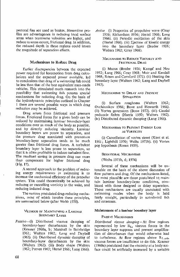
pectoral fins are used as brakes. Streamline pro-files are advantageous in reducing local surface areas when transverse velocities are higher, and reduce to some extent, frictional drag. In addition, the reduced depth in these regions could lessen the magnitude of separation effects.

Mechanisms to Reduce Drag

Earlier discrepancies between the expected power required for locomotion from drag calcu-lations and the expected power available, led to conclusions that drag of a swimming fish could be less than that of the best equivalent man-made vehicles. This stimulated much research into the possibility that swimming fish possess special mechanisms for reducing drag. On the basis of the hydrodynamic principles outlined in Chapter 1 there are several possible ways in which drag reduction may be achieved.

Drag arises from frictional and pressure forces. Frictional forces for a given body can be reduced by maintaining laminar boundary-layer conditions over as much of the body as possible, and by directly reducing viscosity. Laminar boundary layers are prone to separation, and the pressure drag associated with premature boundary-layer separation tends to be much greater than frictional drag forces. A turbulent boundary layer is less prone to separation, so that it is often profitable to induce turbulent flow. The resultant saving in pressure drag can more than compensate for higher frictional drag (Fig. 17).

A second approach to the problem of reduc-ing energy requirements in swimming is to increase the mechanical efficiency of the propeller system. This could theoretically be achieved by reducing or cancelling vorticity in the wake, and reducing induced drag.

The various postulated drag-reducing mecha-nisms, most of which involve these principles, are summarized below (after Webb 1970).

METHODS OF MAINTAINING A LAMINAR • BOUNDARY LAYER

Passive— (i) Distributed viscous damping of boundary-layer disturbances by the skin (Kramer 1960a, b; Marshall in Bainbridge 1961; Walters 1962; Lang and Daybell 1963). (ii) Distributed dynamic damping of boundary-layer disturbances by the skin (Walters 1962). (iii) Body shape (Walters 1962; Purves 1963; Hertel 1966; Lang 1966).

Active — (i) Properties of propulsive wave (Gray 1936; Richardson 1936; Hertel 1966; Lang 1966). (ii) Periodic oscillation of the skin (Hertel 1966). (iii) Ejection of kinetic energy into the boundary layer (Breder 1926; Walters 1962; Gray 1968).

MECHANISMS TO REDUCE VISCOSITY AND FRICTIONAL DRAG

(i) Mucus (Breder 1926; Kempf and Neu 1932; Lang 1966; Gray 1968; Muir and Kendall 1968; Rosen and Cornford 1971). (ii) Heating the boundary layer (Walters 1962; Lang and Daybell 1963).

MECHANISMS TO DELAY AND PREVENT SEPARATION

(i) Surface roughness (Walters 1962; Ovchinnikov 1966; Bone and Howarth 1966). (ii) Vortex generators (Bone 1972). (iii) Caudal peduncle finlets (Harris 1950; Walters 1962). (iv) Distributed dynamic damping (Lang 1966).

MECHANISMS TO PREVENT ENERGY Loss AS VORTICITY

(i) Cancellation of vortex street (Kent et al. 1961; Lighthill 1970; Weihs 1973b). (ii) Vortex peg hypothesis (Rosen 1959).

BEHAVIORAL MECHANISMS

(Weihs 1973b, d; 1974)

Several of these mechanisms will be un-tenable on the basis of the above discussion of flow patterns and drag. Of the mechanisms listed, the most plausible are those postulated to main-tain laminar boundary-layer conditions, corn-bined with those designed to delay separation. These mechanisms are usually associated with swimming modes when the body is held fairly straight, particularly in scombroid fish and cetaceans.

Maintenance of a laminar boundary layer

PASSIVE MECHANISMS

Distributed viscous damping— At flow regimes represented by low R L, viscous forces in the boundary layer suppress and prevent amplifica-tion of disturbances that would otherwise lead to turbulence. At flow regimes above Ri. crib viscous forces are insufficient to do this. Kramer (1960a) postulated that the viscosity at a body sur-face could be artificially increased by a suitable

68

surface covering. He showed experimentally thatsuch a covering could be constructed from arubber diaphragm supported by studs, with thespaces between filled with a viscous fluid. Testsof such a covering on a model showed it behavedlike a rigid surface at low RL. At high RL, therubber diaphragm tended to reduce the magnitudeof a boundary-layer disturbance, and unstablepressure waves caused by a disturbance weretransmitted to the viscous layer where they weresuppressed.

The skin of dolphins is similar in structureto the covering designed to dampen boundary-layer disturbances and Kramer (1960a, b) sug-gested the skin would function in the same way.Kramer (1960a) only tested the covering up toRL of 1.7 X 107, but suggested that disturbancescould be damped at any RL by changing theviscosity of the fluid beneath the rubber dia-phragm. On this basis, Lang and Daybell (1963)suggested that distributed viscous damping couldbe typical of all cetaceans; larger whales swim atspeeds with RL of the order 109.

The only evidence for flow conditions in theboundary layer of dolphins is indirect. Lang andDaybell (1963) measured the drag of a dolphinwith and without a tripping wire fitted aroundthe head. The tripping wire was designed to causecomplete turbulent flow in the boundary layer.The drag was the same with or without thetripping wire, indicating that the boundary layeron the dolphin was normally turbulent. Kramer(1960a) found that his covering was unable toreduce frictional drag for a fully developed,turbulent boundary layer so the skin of thedolphin is not likely to be involved in distributedviscous damping in the proposed manner.

The skin of two scombrid families, Thunni-dae (Marshall, in Bainbridge 1961) and Istioph-oridae (Walters 1962), has a structure similar todolphin skin, and the authors suggested that theskin could function the same as the special cover-ing developed by Kramer. These fish, as well ascetaceans, are able to control body temperatures(Barrett and Hester 1964; Carey and Teal 1969b),and likely the particular skin structure is designedto prevent excessive heat loss (Parry 1949b).

Distributed Dynamic Damping - The trachyp-terid fish, Desmodema, is an elongate fish at least120 em in length, that swims by means of itselongate dorsal fin, and holds the body straightand rigid (Walters 1963). At speeds as low as0.4 Lis, RL is 3.6 X 105, in the critical region fora flat plate. Therefore, transition from laminarto turbulent boundary-layer flow is expected.

The integument of the fish has a subdermalcanal system communicating with the body sur-face by pores. Walters (1963) suggested that highpressure points at a boundary-layer disturbancewould cause the thickening boundary layer tosink through the pores into the canal system. Thiswould prevent amplification of the disturbance.As fluid passed into the canal system, fluid wouldsimultaneously reenter the boundary layer at lowpressure points. In this way, any disturbancewould be damped by spreading its effects overa large area.

Pore canal systems have been reported in ascombrid family, Istiophoridae (Walters 1962).These fish typically swim up to speeds with RLof the order 7 X 107. It is doubtful that a dynamicdamping system could cope with turbulence ofthe order expected at this RL, so this pore systemprobably serves some other function. Ovchinni-kov (1966) suggested that Istiophorids will havea completely turbulent boundary layer.

Body shape - Efficiency of a streamlined bodyin reducing drag depends on two factors, theposition of the shoulder and fineness ratio. Inmost cases, the position of the shoulder is im-portant in defining the portion of the bodycovered by a laminar boundary layer, becausethe shoulder determines the portions of the bodyexperiencing favorable and unfavorable pressuregradients.

In most fish, the shoulder is just behind theopercula (Houssay 1912), which means that asmall proportion of the body experiences afavorable pressure gradient. Under most condi-tions, transition probably occurs at the shoulder,and most of the body would be covered by aturbulent boundary layer.

Bodies of scombroid fish have the shouldersituated far back along the body, at a point 0.6to 0.7 of the length from the nose (Walters 1962;Hertel 1966; Ovchinnikov 1966). This body shapeextends the influence of the favorable pressuregradient, encouraging laminar boundary-layerflow over most of the body. In scombrid fishes,the families Scombridae, Thunnidae, and Kat-suwonidae have body shapes similar to man-madebodies that can maintain a high proportion oflaminar boundary-layer flow to RL of 2 X 106.This is below the RL found at maximum sprintswimming speeds, but these fish often haveadditional drag-reducing mechanisms. The familyCybidae has a different body shape, similar toman-made "laminar" profiles, which can maintaina high proportion of laminar flow up to RL ofthe order of 5 X 107 (Walters 1962).

69

Purves (1963) suggested that dolphins could modify their effective body shape by swimming with the long axis of the body at an angle to the axis of progression. This would reduce RL below RL cru, but the body would not then be stream-lined in the direction of motion. Although a laminar boundary layer might be found on the leading surface, separation would be inevitable on the trailing surface. Evidence for the swim-ming behavior of the closely related porpoise does not support Purves' hypothesis (Lang and Daybell 1963).

Fineness ratio is related more to pressure than frictional drag, although it will affect the magnitude of the pressure gradients and boundary-layer flow (Chapter 1). For streamlined bodies, optimum fineness ratios are recognized depending on whether minimum surface area or volume is required. For fish, the requirement is probably for maximum volume with minimum surface area for which the optimum fineness ratio is 4.5 (von Mises 1945). Variations in fineness ratio between 3 and 7 are associated with pressure drag changes of the order of 10%. Fish and cetaceans swimming in the carangifonn mode with semilunate tail tend to have fineness ratios between 3.5 and 5.0 (Hertel 1966), and fish swimming in the subcarangiform mode obtain values ranging approximately 5.5-7.0 (Hertel 1966; Webb 1971a).

ACTIVE MECHANISMS Properties of propulsive wave — Gray (1936b) suggested that the propulsive wave could assist in stabilizing a laminar boundary layer in dol-phins, and Lang (1966) extended this hypothesis to include all cetaceans. Propulsive movements propel water backward, discharging it into the wake at a velocity slightly higher than that in the free stream. From Bernoulli's theorem, it follows that pressure in the wake will be slightly lower than in the free stream, and would tend to reduce the effects of the unfavorable pressure gradient between the shoulder and trailing edge. This effect must be small, for good propulsive efficiency requires that the velocity increment given to water be as small as possible; otherwise thrust would be associated with high kinetic energy losses.

Richardson (1936) and Hertel (1966) sug-gested that the harmonic nature of propulsive movements could contribute to laminar boundary-layer stability. Schlichting (1968) described secondary steady flow patterns around oscillating cylinders (Fig. 18), but these require that the amplitude of the motion be small in comparison

with the width of the body. In addition, water at some distance from the surface is mainly affected by such motion. As the amplitude of the lateral movements of the body in fish is large, it is unlikely that the harmonic movements promote laminar flow conditions. In practice, they are likely to cause turbulence and separation.

Periodic oscillation of skin — This method of boundary-layer flow control has been suggested by Hertel (1966) and Lang (1966). The hypothesis is that disturbances could be detected and actively damped out by the skin. Hertel noted that no animal had been found with the requisite sensory and muscular system to implement this method. The response time at which such a mechanism would have to operate suggests it is not feasible.

Ejection of kinetic energy into boundary layer — Breder (1926), Walters (1962), and Gray (1968) suggested that the effluent from the gills could act as a source of kinetic energy and be ejected into the boundary layer to reduce or prevent transition.

Observations made by Allan (1961) showed that, for small fish at least, the gill effluent was a source of turbulence, rather than a turbulence-reducing mechanism. The same observations were reported by Walters (1962) for small fish. Walters considered that kinetic energy in the gill effluent could still be used as a drag-reducing mechanism in fish that used ram ventilation during swim-ming, when the opercula would function like slots on airfoils. In ram ventilation, injection of the gill effluent into the low momentum, reduced-flow areas of the boundary layer could prevent or delay both transition and separation.

Reducing viscosity and frictional drag

Mucus

It was originally thought that mucus could reduce drag by virtue of its slippery nature (Breder 1926; Kempf and Neu 1932). Hydro-dynamic theory predicts this is not possible, as there is no slip between fluid interfaces, just as there is none between a solid–liquid interface (Richardson 1936; Gero 1952).

It is well known that the addition of small quantities of long chain, high molecular weight polymers to the boundary layer can reduce drag under turbulent boundary-layer conditions (Lumley 1969). For example, Gadd (1966a, b) found that 10 ppm of such a polymer (polyethy-lene oxide) could reduce frictional drag by 40%.

70

Lang (1966), Muir and Kendall (1968), andLighthill (1969, 1971) suggested a similar hydro-dynamic function for mucus, which is a long-chainpolymer.

Rosen and Cornford (1971) tested dilutesolutions of mucus from several species of fishin a rheometer. RL exceeded critical values.Variable results were obtained; some mucussolutions reduced resistance, but others had noeffect. Nor were mucus solutions giving the great-est decreases in resistance necessarily from fishwith the highest swimming speeds. In fact, theopposite was also found. From Rosen andCornford's results it seems probable that mucusdoes have a drag-reducing function, similar toman-made, long-chain polymers. The variance inresults may be related to the amounts of mucusobtained, which were not quantified.

Kowalski (1968) and Dove and Canham(1969) reported results of trials using polyox toreduce the drag of ships. Greatest drag reductionwas found when the polymer was introducedinto the boundary layer at small angles of inci-dence, in a pu]satile fashion and at a point nearthe shoulder. These conditions are often fulfilledby the opercular slits of fish. Gills are typicallyrich in mucus cells (Hughes and Grimstone 1965;Muir and Kendall 1968; Hughes and Wright1970). In addition, production over the wholebody surface could introduce mucus into theboundary layer, but its effectiveness would possi-bly be reduced by the rate of diffusion of the largemolecules.

A third means by which mucus could reducedrag has been suggested by Breder (1926). Hesuggested that mucus could fill in irregularitieson the surface, and reduce surface roughness orimprove streamlining.

HEATING THE BOUNDARY LAYER

Cetaceans, some lamnid sharks, and scom-brids maintain body temperatures fairly constantabove the ambient water temperature (Barrettand Hester 1964; Carey and Teal 1969a, b; Careyand Lawson 1973). Walters (1962) and Lang(1966) suggested that these animals could heatthe boundary-layer water, reducing its viscosity.In practice, such a mechanism is unlikely; ceta-ceans are covered by an insulation layer (Parry1949a), and scombrids often have similar oilylayers in the skin (Marshall in Bainbridge 1961).

It would also be impractical to warm up theboundary layer. Carey and Teal (1969b) reported amaximum temperature difference of 15 C betweenthe body temperature of skipjack tuna at 30 C

and the ambient water at 15 C. Under these con-ditions, the maximum decrease in friction dragwould be 14%, providing the boundary layer washeated to the body temperature instantaneously.Walters (1962) considered this would not bepossible, as the water would only be in contactwith a fish for a short period of time. For a 2kg tuna, Walters calculated that contact wouldlast 0.1 s. It can be shown that the amount of heatrequired to obtain a 14% reduction in drag for a2 kg tuna would be about 25 kcal Is, approximatelyhalf the thermal capacity of the body.

It can safely be concluded that heating theboundary layer as a method of reducing drag isnot used.

Delay and prevention of separation

SURFACE ROUGHNESS

Some fish have roughened body surfaces,apparently to induce transition, delay separation,and reduce pressure drag. Walters (1962) de-scribed a corselet of scales and thickened skinnear the shoulder of the scombrid familiesCybidae, Thunnidae, and Katsuwonidae, whichmight act the same as a tripping wire. It is morelikely that this represents faring of the body toaccommodate the pectoral fins.

The scombrid families Xiphiidae (swordfish)and Istiophoridae (sailfish) have poorly stream-lined bodies in comparison with other scombrids.Neglecting the rostrum, the shoulder is close tothe front of the body and a large proportion ofthe body will experience an adverse pressuregradient (Ovchinnikov 1966). The presence of therostrum results in an extended concave surfacepresented to the incident flow, so that a laminarboundary layer would be difficult to maintainover the remainder of the body (Walters 1962).

Ovchinnikov (1966) calculated that therostrum of the swordfish, Xiphias gladius, islong enough for transition to occur at low swim-ming speeds. As a result the body would be sweptby a more stable turbulent boundary layer. Thesailfish, Histiophorus arnericanus, has a shorterrostrum, so transition would only be expected athigher swimming speeds. However, the rostrumhas fairly large protuberances, which would pene-trate the boundary layer and induce transition atlow speeds. Both fish are undoubtedly swept byturbulent boundary layers, tending to offset theapparently poorly streamlined body by reducingthe tendency for separation.

Bone and Howarth (1966) suggested that theboundary layer on dogfish would tend to separate

71

during swimming. They considered that the den-ticles would induce turbulence in the boundary layer, and offset the tendency for separation.

VORTEX GENERATORS

Ruvettus pretiosus, the castor oil-fish, has a special integument which probably functions to generate vortices that not only induce, but main-tain, a turbulent boundary layer (Bone 1972). The integument contains an extensive system of sub-dermal canals communicating with the surface by caudally-directed pores. The integrity of the subdermal canal system is maintained by spe-cialized ctenoid scales, which have projections well beyond the body surface. Bone guessed that the fish would swim at speeds to about 5 L/s, when RL would be of the order of 1.7 X 107 . At this RL turbulent boundary-layer flow is expected and it is doubtful if the canal system would operate like the distributed viscous damping system of Desmodema (Walters 1963).

Bone suggested that vortices generated at the tips of the scales would ensure a turbulent boundary layer, and, because the vortices would be directed backward and toward the surface, they would continually replenish the boundary layer with energy derived from the outer flow assisting the maintenance of an attached boundary layer.

Bone also noted that oscillation of the body of a dead fish, similar to that expected during swimming, caused fluid to be ejected through the pores of the canal system. This might serve as an additional source of kinetic energy for the boundary layer, or to improve turbidity.

CAUDAL PEDUNCLE FINLETS

Finlets are present on the caudal peduncle of all scombrids (Walters 1962) and a fossil shark, Diademodus hydei (Harris 1950). The finlets are too small to serve a direct propulsive function. Harris and Walters compared the finlets with multiple wing-tip slots often used on high-lift aerofoils. The finlets probably redirect the flow of water over the caudal peduncle, deflecting it along the body rather than permitting normal flow which could lead to separation (Wu 1971b, c).

DISTRIBUTED DYNAMIC DAMPING

Lang (1966) suggested that the special skin structure of dolphins may not be associated with maintainance of laminar boundary-layer flow. Instead, the skin may be designed to stabilize turbulent boundary-layer flow and prevent separa-tion of this turbulent boundary layer.

There is no evidence for or against such a mechanism. A swimming dolphin is expected to have a turbulent boundary layer, separating at some point beyond the shoulder, but before the trailing edge. This is especially so for dolphins (compared to other vertebrates swimming in the ca.rangiform mode with sernilunate tail) because of their high amplitude movements (Slijper 1958, 1961; Lang and Daybell 1963). Observations made by Steven (1950) showed that separation does not occur. Steven observed that the only disturbance caused by dolphins swimming in phosphorescent seas was two diverging lines. These were probably caused by tip vortices around the tail flukes. A separated boundary layer would have been indi-cated by a broad path of disturbances, as Steven observed for seals.

Prevention of energy loss as vorticity

CANCELLATION OF VORTEX STREET

Kent et al. (1961) suggested that a Karman vortex street would be produced behind the head of a swimming fish. They considered that a second series of vortices would be produced at positions of maximum amplitude of the tail, and the two series could cancel out to prevent energy losses to the wake.

This would only be feasible if the frequency of vortices in each series was the same. The frequency of vortices in a Karman street, f„, can be calculated from Equation 26, taking the Strouhal Number as 0.2. The frequency of tail vortices will be equal to twice the tail-beat frequency, which can be calculated from equations in Table 2. Consider a 30 cm trout, in which the width of the head would be about 0.1 L. The ratio between the two frequencies will be closest at highest swimming speeds, about 300 cm/s (10 L/s). 2 f would be 29.3 with f. 20.0, so under optimum conditions, the maximum drag saving could be of the order of two-thirds.

However, it is unlikely that a vortex street of the type considered by Kent et al. (1961) would be generated behind the head of a fish even when swimming, and the pattern of the vortex street generated by the tail may not be of the nature required. Experiments by Hertel (1966) indicated that a caudal fin will generate stable vortex streets only at some speeds, and often the street will be a single row. Although this has not been confirmed for fish throughout their normal swimming range, it seems unlikely that drag of individual fish would be reduced in the manner proposed by Kent et al. (1961).

72

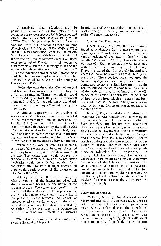
Alternatively, drag reductions may be possible by interactions of the wakes of fish swimming in schools (Breder 1926; Belyayev and Zuyev 1969; Zuyev and Belyayev 1970; Weihs 1973b). Typically, schooling fish are of similar size and swim in horizontal diamond patterns (Keenleyside 1955; Nursall 1973). Weihs (1973b) stated, "In this formation, when the lateral dis-tance between adjacent fish is twice the width of the vortex trail, wakes between successive lateral rows are cancelled. The third row will encounter a uniform flow and the total energy saving to the school is half the relative gain to the second row." This drag reduction through school interaction is predicted by idealized hydromechanical model-ling, so the actual energy loss would probably be lower (Weihs 1973b).

Weihs also considered the effect of vertical and horizontal interaction among schooling fish on thrust generation. Thrust theoretically could be increased by at least 10% in the horizontal plane and to 30% for an optimum vertical distri-bution, but without any attendant changes in kinematics.

A different approach to the problem of vortex cancellation for individual fish is included in the hydromechanical models developed by Lighthill (1970) and Wu (1971b, c). A vortex sheeti produced downstream by the trailing edge of an anterior median fin or inclined body edge could be resorbed on the leading edge of the next posterior median or caudal fin. The importance of this depends on the distance between the fins.

When the distance between fins is small, as in most fish swimming in the anguilliform and subcarangiform modes, a vortex sheet would fill the gap. The vortex sheet would behave me-chanically the same as a fin, and the propulsive mechanics would be equivalent to that for a continuous fin. However, a slight decrease in drag would result because of the reduction in fin area by the gaps.

When gaps between the fins are large, the relative motions of the interacting edges will also be increased because of the nature of the propulsive wave. The vortex sheet could still be resorbed at the leading edge of the posterior fin with no addition to energy loss in the wake. If the phase difference between the motion of interacting edges was large enough, the thrust work done would not be entirely cancelled by resorbtion of the vortex sheet on a downstream posterior fin. This would result in an increase

IThe difference between vortex streets and vortex sheets is discussed in Chapter 1.

in total rate of working without an increase in wasted energy, technically an increase in pro-peller efficiency (Chapter 5).

VORTEX PEG HYPOTHESIS

Rosen (1959) observed the flow pattern found some distance from a fish swimming at sprint speeds. Cross flows around the dorsal and ventral surfaces of the body produced vortices on alternate sides of the body. The vortices were not part of a Karman street, but were associated with thrust rather than drag (Lighthill 1969). Rosen postulated that fish actively induced and energized the vortices so they behaved like quasi-static pegs. These vortices were then used the same as rigid pegs (Gray 1957b); they were also considered to act as rollers between which the fish was pushed, the scales rising from the surface of the body to act as vanes improving the effi-ciency of the action. The fish left behind a line of free vortices from which all energy had been absorbed; that is, the total energy in a vortex was the same as that in an equivalent mass of the free stream.

Rosen (1959) concluded that the drag on a swimming fish was virtually zero. However, his experiments detected the flow at some distance from the fish, and because high propulsive efficiency requires that velocity increments given to the water be low, the true original movements of the water were undoubtedly obscured (Aleyev and Ovcharov 1969, 1971). In addition, Rosen's conclusion does not take into account the degra-dation of energy that must occur with each transformation, nor does it fit the observed physi-ology of swimming fish. Furthermore, it is most unlikely that scales behave like vanes, in which case there would be relative flow between the surface of the fish and the vortices. The velocity of flow adjacent to the fish in the vortex would tend to be higher than that of the free stream, so this motion would be expected to result in a higher drag than otherwise anticipated. In view of these objections, the vortex peg hy-pothesis is unlikely.

Behavioral mechanisms

Weihs (1973b, d; 1974) described several behavioral mechanisms that can reduce drag or net thrust required to swim at a given mean speed. Energy savings through the cancellation of vortex sheets in some schooling fish is de-scribed above. Weihs (1974) has also shown that routine activity interspersing glides with short bursts of activity (burst/ glide behavior) can

73

decrease the energy required to traverse a givendistance in a given time by over 50% comparedto swimming at constant speed. Alternatively,under optimum burst/ glide conditions rangemay be increased by a maximum of three times.Negatively buoyant fish could achieve similarenergy economies by gradually gliding to alower depth and then rapidly swimming upwardsto the original depth (Weihs 1973d).

Discussion

Only a few of the proposed drag-reducingmechanisms appear plausible, mainly those withanalogies in aircraft industrial practices (vonMises 1945; Schlichting 1968). Each mechanismhas been considered on its own merits, and nonehave been rejected because there is no man-madeequivalent (e.g., distributed viscous damping forturbulent boundary-layer control). The list ofdrag-reducing mechanisms reflects current indus-trial thinking; in all probability there are othernovel mechanisms yet to be recognized.

Most of the plausible drag-reducing mecha-nisms have limited general application to aquaticvertebrates, often being associated with sometaxonomic group and its swimming mode.Distributed viscous damping for turbulentboundary-layer control would have a cetaceanmonopoly with the possible exception of oil-filled canal systems in marlin (Marshall inBainbridge 1961). Distributed dynamic dampinghas only been reported in Desmodenra but ispossibly typical of trachipterid fish (Walters 1963).Vortex generators in Rrrnettus may have widerapplication (Bone 1972).

Plausible drag-reducing mechanisms forboundary-layer control are commonly found infish swimming with the body fairly straight.These mechanisms tend to be associated withcertain swimming modes. Fish possessing thesedrag-reducing mechanisms are also those towhich theoretical and dead-drag calculationsare most likely to give reasonable measures ofswimming drag. Drag-reducing mechanisms thatfollow industrial practices are most easily recog-nized in these fish.

By contrast, surface roughness (includingvortex generators), vortex cancellation in schools,and vortex sheets filling fin gaps are largelyrelated to other swimming modes when the bodyand/or median fins execute large amplitudemovements for much of their length. Problemsrelating to premature separation are then ofparamount importance. Vortex sheets filling fin

gaps apply to anguilliform-type propulsion

(including subcarangiform motion). The onlyexceptions appear to be sailfish and swordfish,when turbulence in the boundary layer is inducedin response to special body shapes, rather thanswimming mode.

Mucus is potentially the most universaldrag-reducing mechanism, with the exceptionof cetaceans. However, mucus reduces frictionaldrag in a turbulent boundary layer, and mayapply more to anguilliform-type propulsion thanother modes. This is because the more advancedcarangiform modes and other modes when thebody is held more or less straight, are probablyassociated with a larger proportion of laminarflow over the body.

The probable effectiveness of most drag-reducing mechanisms can readily be appreciated.The advantages of different flow regimes can beshown by calculation (Fig. 17). The potential ofmucus (60% reduction in frictional drag) isshown by empirical observations (Rosen andCornford 1971). Distributed viscous dampingfor turbulent boundary-layer control is an un-known factor, but its advantages would beimmense if separation were avoided. Thesemechanisms make large reductions in some dragcomponent, which is also a substantial reductionin total drag.

A possible exception is the distributeddynamic damping system of Desmodenta (Walters1963). Because this fish swims in the amiiformmode, high drag costs are expected from theanguilliform-type motion of the dorsal fin. Inthis case, the frictional drag of the fairly straightbody would probably represent a small portionof the total drag. Thus, the reduction in dragthrough the maintenance of laminar boundary-layer flow over the body would be small in rela-tion to total drag, with consequent small energeticsaving.

The various drag-reducing mechanisms arenot likely to apply at all swimming speeds. Thespecial body shapes of scombroid fish and ceta-ceans only maintain a high proportion of laminarflow at regimes with RL between 2 and 5 X 107,whereas maximum speeds occur with RL of theorder 7 X 107. Similarly, Desmodenta's distributeddynamic damping system would be ineffectivewith intensity of turbulence at high speeds. Incontrast, surface roughness could be effective atall speeds, but at higher speeds early transitionwould be expected in any case. Mucus could bemore effective at higher speeds in large fish whentransition occurred at progressively more anteriorpositions, but in most fish transition is likelythrough other causes at lower speeds, in which

74

case mucus would apply equally here. Vortex sheets filling fin gaps are part of the thrust mechanism, and would operate at all speeds. In general, it appears that drag-reducing mechanisms apply mainly to cruising speeds and lower sprint speeds. Most fish activity will be in this area, simply because the metabolic machinery cannot cope with continual high speeds. Thus, drag savings apply to those activity levels when energetic expenditure will be highest in the long term.

A further reason for the operation of drag- reducing mechanisms at lower speeds would be

applicable if high-speed sprints were associated more with the work required to overcome the inertia of the body and added mass rather than drag caused by boundary-layer effects. In this case, it is possible that a series of further drag-reducing mechanisms could be identified in rela-tion to reducing the total mass that must be accelerated. Perhaps the more cylindrical bodies of fish like pike, which attack prey by sudden darts, is associated with lower added mass than the more elliptical bodies of fish like carp, brows-ing on the bottom. This is in the realm of specula-tion with no evidence for support.

75

Chapter 5 - Thrust and Power

Introduction

The preceding discussion on the use of dragmeasurements to calculate swimming powerreveals several disadvantages, both in theory andpractical measurement techniques. Consequently,it is advantageous to measure thrust, because,being equal to total drag, it will include any grossflow effects, interactions, and drag-reducingmechanisms (without identifying them) that dragcalculations or measurements do not include.

A few attempts have been made to measurethrust power directly (Houssay 1912; Gero 1952;Lang and Daybell 1963; Gray 1968). Most wereconcerned with peak power levels for sprints orfish jumping from the water and often only aportion of the total power was measured. It isdifficult to relate such measurements to anyparticular swimming speed, and it is not possibleto construct any relation between thrust powerand speed.

The most satisfactory means of direct cal-culation of thrust and power output would befrom a complete description of the flow arounda swimming fish at different speeds. This wouldrequire an exorbitant amount of work. At thepresent time, flow has only been described quali-tatively for the boundary layer (Allen 1961) andouter flow some distance from the fish (Houssay1912; Gray 1936b; Rosen 1959; Aleyev andOvcharov 1969, 1971) at a few swimming speeds.

Indirect approaches to calculate thrust andpower are, therefore, likely to be of greater valuein fish propulsion energetics studies at the presenttime. Of indirect approaches, the developmentof suitable hydrodynamic models is of greatestimportance. Other approaches using mechanicalmodels (Breder 1926; Gray 1936b; Kramer 1960;Kelly 1961; Smith and Stone 1961; Hertel 1966;Pyatetskiy 1970b; Siekmann 1963) or relationsbetween added drag loads and kinematics (Webb1971a) are by comparison of limited applicationand mainly important in testing, or giving addi-tional input to models of wider application.

Hydrodynamic models have always beenimportant in the study of fish locomotion. Theywere initially used qualitatively to show that the

observed movements executed by swimming fishwould generate large thrust forces, and to evalu-ate the kinematic requisites for the generation ofthrust (Gray 1933a, b, c, 1953b, 1968; Harris1937; Breder and Edgerton 1942; and others) orto elucidate the distribution of thrust (Bainbridge1963).

Further expansion of these qualitativemodels into a quantitative fornl has generallyproved difficult, not only because of the detailedmeasurements required in their application(Taylor 1952; Gray 1953b) but because they arebased on too great an oversimplification of thepropulsive system, particularly in neglectinginteraction between segments.

Many of these problems also apply to modelsoriginally developed in quantitative form (Webb1971a). Recent models have been proposed thatcan either be reduced to simple terms related toeasily measurable key kinematic parameters, orpredict some form of thrust coefficient similarlybased on measurable kinematic parameters (Light-hill 1960, 1969, 1970, 1971; Wu 1961, 1971a, b, c;Weihs 1972, 1973a). These models hold thegreatest potential for application to a wide rangeof fish energetics problems.

Direct Measurements of Power Output

The most comprehensive series of power out-put measurements were made by Houssay (1912),for fish of various sizes from 18 species. Each fishwas attached to a balance so that as it swam itwas forced to lift weights of various sizes. Thepower developed by the fish was calculated fromthe product of the mass lifted and the distance itwas raised. Only part of the work done by thefish was measured. Work to overcome: (1) dragof the fish, (2) drag of the balance, (3) inertia ofthe balance, and weights a distance from the ful-crum, (4) friction in the balance was unaccountedfor. In addition, fish were forced to swim in atight arc, which undoubtedly reduced their per-formance (Bainbridge 1963).

Gero (1952) calculated the power requiredduring acceleration of a perch from a standingstart, and for a porpoise jumping from water. It

77

• • ■o'

is not known if these animals were then developing maximum power. The power developed by a por-poise during acceleration was also measured by Lang and Daybell (1963).

Gero (1952) also measured the thrust and power output of several fish attached to a fishing line. The strain was measured on the line as the fish swam away from a boat. Gero pointed out that only power in excess of the drag power for the fish and line was measured. He also noted that measurements were subject to error if the fish swam at an angle to the line and boat, and that the line must have interfered with the fish.

Despite their recognized inaccuracies, the above measurements of thrust and power are the only ones available. They are given in Table 6. The measured power output is compared to estimated values based on information for verte-brate muscle systems and expected caudal pro-peller efficiency. Thus, a muscle power output of 8 X 10 5 erg/ s per g was taken for cold water fish, and 40 X 10 5 erg /s per g for mammals (Bainbridge 1961). The latter figure applies to cetaceans, and possibly Gero's (1952) sharks, grouper, and barracuda if they can control their body temperatures. It was assumed that half the body mass was propulsive muscle, half of which works at any instant, and that caudal propeller efficiency was 0.75.

Estimated power outputs are up to an order of magnitude greater than measured values, with a greater difference for smaller than larger animals (Fig. 47). The difference may largely be attributed to unmeasured power output in the experiments. For example, in Houssay's experiments, some portion of the unmeasured work depended on the design of the balance, and consequently this por-tion would have represented a relatively greater proportion of thepotential maximum power output of smaller fish than larger fish. In general, there is agreement between measure and calculated propulsive power output values.

Hydromechanical Models and Indirect Measurements

The basis for descriptions of kinematics in fish propulsion is the identification of arbitrary segments, regarded by Gray (1968) as "the funda-mental unit of aquatic undulatory propulsion." This concept applies also to models relating the kinematics to thrust production, the application of various models differing to a large extent in the emphasis given to different segments. Models that assume segments may be compared to

hydrofoils tend to consider all segments (Taylor 1952). Others who consider reaction forces asso-ciated with virtual mass effects also consider all segments, but can relate bulk energy changes to a single segment at the trailing edge, with conse-quent emphasis there (Lighthill 1969, 1970, 1971, 1972; Wu 1971a, b, c).

Apart from this basic similarity, hydro-mechanical models can be divided into two main groups, depending on certain assumptions made in their formulation. These are summarized in Table 7 for various quantitative models. The two assumptions consider either resistance forces or reaction forces to be dominant. In the former, instantaneous forces acting on a segment are regarded as resistive forces depending only on the segment's resultant velocity at some angle of attack to the incident flow. This approach is sometimes called quasi-static, as it also assumes that the forces acting on a segment at any instant are the same as those acting under equivalent steady-state conditions of velocity and angle of attack. The net effect of the motion of any segment during a cycle is the sum of the steady-state forces for all instances in that cycle (Gray 1953b).

The reactive force approach considers the inertial forces acting on a segment. These forces

WCILM7 - g

FIG. 47. Maximum measured power output of fish and cetaceans as a function of weight. Solid circles show values calculated for 17 species of fish from data in Houssay (1912), solid squares for three species of fish from data in Gero (1952), open squares and open circles for cetaceans from data in Gero (1952) and Lang and Daybell (1963) respectively. Solid lines represent estimates of muscle power output expected for fish and mammals. Further explanation is given in text and Table 6,

78

Scyliorhinus canicula

Esox lades

760 6.38 X 10 6 590 5.29 X 106

590 2.58 X 106 540 2.47 X 106

1,525 5.62 X 10 7 620 3.03 X 107 440 2.42 X 107 59 2.02 X 106

Negaprion 36,774 2.83 X 109 brevirostius

Promicrops 7,718 8.60 X 108 itaiara

SPhyraena 11,350 3.92 X 109 barracuda 9,080 6.04 X 109

TABLE 6, Values for highest power outputs of fish and cetaceans, from direct measurements. For reasons discussed in text these are probably not maximum power outputs of the various species.

Weight Power output Weight Power output Species (g) (erg/s) Reference Species (g) (erg /s) Reference

Merlangus Alburnus 40 6.04 X 10 5 Houssay pollachius 530 2.63 X 107 Houssay lucides 32 2.50 X 105 (1912) (? whiting) 405 2.02 X 107 (1912) 15 1.24 X 105

150 1.20 X 107

135 8.53 X 106 Barbus 548 1.33 X 107

75 3.18 X 106 fluviatilis 240 6.61 X 106

Labrits 322 1.87 X 107 Scardinius 205 5.03 X 106 bergylta 180 8.20 X 10 6 erythroph- 180 2.40 X 106

100 4.27 X 10 6 thalmus

Pagellus 312 1.12 X 107 Cyprinus 1,628 4.34 X 107 centrodentus carpio 498 9.94 X 106

320 5.37 X 106 235 2.10 X 106

Cottes 68 1.04 X 106 171 7.92 X 105 bulbalis 28 4.44 X 105

Time 732 1.61 X 107 Platessa 710 1.29 X 107 vulgaris 376 6.80 X 106

vulgaris 80 2.41 X 106 23 2.00 X 105 50 7.32 X 105

Gobio 35 2.56 X 105 Crenilabrus 40 2.25 X 105 fieviatilis 21 1.00 X 105

melops Leuciscus 159 1.71 X 106

Raja punctata 1,863 4.02 X 107 rutilas 90 1.02 X 106 and R. 1,570 4.13 X 107 44 2.86 X 105 elevate 1,132 4.49 X 10 7

730 1.30 X 107 Perca 109 3.44 X 107 Gero

490 1.15 X 10 7 j7avescens (1952) 272 2.70 X 10 7

195 2.49 X 106 Charcharhines 26,332 1.93 X 10 9

50 2.67 X 105 leucas 9,534 9.30 X 108

Tursiops 431,300 1.13 X 10 11 Salmo iridees 633 1.30 X 10 7 truncates

590 1.86 X 107

585 1.71 X 107 Lagenorhyn- 90,800 1.27 X 10 19 Lang and

317 1.40 X 107 chus Daybell

125 4.27 X 106 obliquidens (1963)

79

TABLE 7. Models of propulsion for fish and cetaceans. Key to swimming modes: A = anguilliform;C = carangiform; CST = carangiform with semilunate tail; O= ostraciform; R = rajiform.

Amplitude Flow restrictionsSwimming of lateralmode movements Dimensions Separation Notes

HydromechairicalResistive (quasi-static)

lifting wing theoryO,CST small 2 yes

CST large 2 yesCST large 2 yes

Alifting cylinder theory

large 3

A large 2

Reactive (inviscid)slender body theory

A small 2

A,C small 2

C large 2

C large 2

A

A,R small 2C small 2

lifting wing theorysmall 2

yes amplitude constantalong body length.

no 11

no amplitude increasesalong body length.

no amplitude increasesalong body length;separation discussed.

no amplitude increases(discussed) along body length.

no acceleration.(discussed)

no amplitude increases

nono

A small 2

A,C small 2

R small 2

CST large 2C, CST small 2

AVariousO

A,R

A

small 2

large

large

large

large

no

along body length.

11

no as above; bodythickness effectconsidered.

no amplitude increases

nonono

along body length;high RL,

amplitude increasesalong body length;body thickness effectsconsidered.

Mechanical

- amplitude constant.

- amplitude constant.

- amplitude increasesalong length.

Reference

von Holste andKuchemann (1942)Parry (1949a)Gero (1952)

Taylor (1952)

Gray (1953b)

Gadd (1952, 1963)

Lighthill (1960,1969, 1970)

Lighthill (1971)

Weihs (1972, 1973a)

Smith and Stone(1961)

Siekman (1962, 1963)Bonthron and Fejer

(1963)Pao and Siekman

(1964)Uldrick andSiekman (1964)

Wu (1961, 1971a,b)Kelly (1961)

Lighthill (1969, 1970)Wu (1971b,c)Wu and Newman

(1972)Newman and Wu

(1973)Newman (1973)

Gray (1936b)Kramer (1960)Breder (1926)Hertel (1966)Kelly (1961)Siekman (1963)Smith and Stone

(1961)

80

are proportional to the rate of change of resultant velocity, and the virtual mass associated with a segment's motion (see particularly Lighthill 1970).

Each main group can be subdivided de-pending on the type of hydromechanical theory, whether for slender bodies or lifting wings.

In his survey of aquatic animal propulsion, Lighthill (1969, 1970) showed that the two hydromechanical approaches have different areas of application. For small animals with RL < 1, resistive theory is applicable, and this probably applies to RL = 103 when there is no particular lateral flattening of the animals, as in many invertebrates. For vertebrate propulsion, lateral flattening is normal. This substantial increase in depth is associated with large virtual mass effects during swimming, so that resistance forces tend to be small in comparison with reaction forces (Lighthill 1970). This also applies in any case when RL > 103 .

There will, of course, be intermediate forms expected to use a combination of resistive and reactive forces. Lighthill (1970) considered this to be the case for eellike fish, where lateral compression has not progressed to the same extent as fish swimming in other body modes.

A further difference between resistive and reaction approaches is the "fluid" to which the models apply. The use of quasi-static resistive theory permits analysis of locomotion in a real fluid. In fact, segments may be compared to hydrofoils so that the various forces acting at any instant may be computed from empirical observa-tions of mechanically similar systems. Motion in a real fluid includes boundary-layer growth and separation effects but neglects interaction between segments. In contrast, reaction forces have been analyzed for inviscid fluids that do not initially take into account forces of viscous origin. Lighthill (1960, 1970) set out a preliminary consideration of the effects of such forces, which are likely to be most relevant in anguilliform propulsion.

A common difficulty with most models is expressing kinematics in suitable mathematical terms. The usual assumption is that segments move with simple harmonic motion, and as seen in Chapter 2, this is not strictly so. Differences between simple harmonic motion and observed motion are small (Gray 1933a). In addition, the practical difficulties encountered in measuring any kinematic parameter mitigate against too rigorous an application of this objection.

Kinematic variation occurs at all levels with different species, individuals, and time (Nursall

1958b) and has effects on thrust that are difficult to determine. The most sensible method of overcoming this problem is to use a quasi-static approach to consider detailed movements of segments. When used in most resistive models this tends to ignore segmental interactions (Gray 1933a, 1953b), but can be used successfully with reaction models considering a trailing-edge segment (Lighthill 1971). Another practical difficulty is encountered, for involvment in a comprehensive analysis of this nature requires an immense amount of work (Taylor 1952; Gray 1953b). Taylor considered that the inherent variation in propulsive movements would prob-ably prevent the measurement of "sufficiently realistic values" for kinematic parameters.

The problem faced by the biologist who wants to use hydromechanical models to calculate thrust and power in swimming fish is "which one to use." This will depend on several factors, such as swimming mode, his primary area of interest (mechanics or energetics, etc.). In general, a re-action model is likely to be most important, and then one that considers energy changes in terms of key kinematic parameters, measurable with some accuracy and repeatability. In this respect, key parameters may be identified as the wavelength of the propulsive wave, XB, tail-beat frequency, f, and amplitude, A (Webb 1971a, 1973a). Key kinematic parameters dictate fixed relations between body movements and resultant velocity, angle of attack, etc., during propulsive cycles. They will also reflect the mean propulsive effort of a fish, with results similar to a more detailed analysis of the quasi-static type (Lighthill 1970, 1971; Wu 1971a, b, c).

Qualitative quasi-static models

With the exception of body swimming modes, most swimming movements have only been considered in qualitative form at the present time. This approach to the motion and forces for various segments was used in all earlier work on fish locomotion, beginning with Borrelli (1680), Pettigrew (1873), Marey (1874, 1895), Breder (1926), and particularly Gray (1933-1968). Bainbridge (1963) extended quasi-static ap-proaches for hydrofoils to estimate the importance of various segments along the body in generating thrust for Ambramis, Carassius, and Leuciscus (subcarangiform mode). Bainbridge assumed thrust proportional to the square of the local transverse velocity (W 2) and local area. Angle of attack was assumed positive at all times, and variations along the length of the body were

81

neglected. Bainbridge's estimates suggested that the caudal fin would generate 45, 65, and 84% of total thrust in Ambramis, Carassius, and Leuciscus, respectively. This follows a trend toward concentration of significant lateral move-ments to the posterior of the fish, so that Ambramis kinematics tended more to anguilli-form propulsion, and Leuciscus more to carangi-form propulsion.

Paired and median tin propulsion and ostra-ciform propulsion have only been discussed qualitatively, with the exception of the rajiform mode (Wu 1961, 1971a; Kelly 1961; Siekmann 1962, 1963). Movements of the caudal fin in ostraciform propulsion, and pectoral fins in labriform propulsion have been envisaged gener-ating thrust the same as a fan (Harris 1937; Gray 1968). Positive thrust appears to be generated throughout a cycle from a combination of resis-tive and reactive forces (Gray 1968).

For other fin modes, when the base of the fin is relatively large and specific wavelengths small, longitudinal forces in the direction of the fin base are generated the same as anguilliform propulsion. Because the fins are attached at their bases to the body, forces are also generated normally to the fin base (Harris 1937; Breder and Edgerton 1942). Similar forces are generated to those of the fins used in ostraciform and labri-form modes. In the case of pectoral fin move-ments, such forces will be associated with yawing couples, cancelling out for symmetrical move-ments of both fins. Asymmetrical movements between pairs of fins contribute significantly to maneuverability.

Forces generated normally to the long axis of median fins contribute to thrust when the fins are set backward at an angle to the body axis as in Monocanthus (Harris 1937). The kinematics of these fins will be associated with pitching couples, again cancelling out for symmetrical movements when the fins occur in pairs, as in balistiform propulsion. The situation in gymnotiform and amiiform propulsion is uncertain, as the median fins are not found in functional pairs. Forces generated normal to the fin's long axis would be expected to cause the animals to rise or fall in the water as they move forward. The effect of such forces could be counteracted by appropriate buoyance mechanisms, or a large number of wave-lengths along the fin.

The long pectoral fins of skates probably function the same as long median fins in similar modes. Yawing forces generated by these fins would be cancelled out during normal forward propulsion because the structures are paired.

Quantitative models

Quantitative models are presently restricted to anguilliform and carangiform propulsion. Wu's (1961, 1971a) model is an exception, appli-cable to rajiforrn propulsion, but there are no data. The kinematic data available for input to body swimming mode models are also limited to steady2 swimming at speeds maintained for at least a second. Higher speeds undoubtedly in-volve predominantly acceleration phenomena and this may be treated by a modification of a basic model (Weihs 1972, 1973a).

In the following discussion of quantitative models, steady swimming for each of the main body swimming modes will be considered. Sub-sequently the available information on accelera-tion and steady-state models will be combined in an attempt to predict acceleration energy expenditure.

A resistance and a reaction model is con-sidered for each mode, with numerical solutions calculated for each. However, only one example of each is considered, selected from those sum-marized in Table 7. Selection was based on a model's value in biological situations. For most body swimming modes, the resistance model proposed by Taylor (1952) is discussed. This model has the advantage over others because it considers three-dimensional flow, and is conse-quently most realistic. It is also in a form that can be easily applied to real fish-type motions. Of reactive models, that proposed by Lighthill (1969, 1970, 1971) is considered most appropriate.. In detailed form, it is descriptive of real fish motions, and can be simplified to a form relating to key kinematic parameters without substantial loss in accuracy. It discusses forces of viscous origin, and furnishes hydromechanical explanations for much of the morphological variability observed among fish. The conclusions given by Lighthill's models have almost simultaneously been obtained by Wu (1971b, c). However, these latter models require the use of thrust-related coefficients making them of less immediate biological use.

A special lifting-wing model is required to describe carangiform propulsion with semilunate tail. All relevant models proposed to date require the use of thrust-related coefficients. The models proposed by Parry (1949a) and Lighthill (1969, 1970) are discussed. Additional relevant calcula-tions were set out by Wu (1971b, d).

2Time independent.

82

Steady Swimming

Anguilliform propulsion

RESISTIVE (QUASI-STATIC) MODEL

Taylor (1952) considered resistance forcesacting on a long narrow smooth cylindrical body,each segment of which executed simple harmonicmotion of constant large amplitude. Flow wasassumed to be laminar. The motion of a segmentwas considered quasi-statically. Its instantaneousmotion was compared with steady flow aroundinclined cylinders under equivalent conditions foreach segment. Empirical data for lift (thrust) anddrag forces on such cylinders, at different flowvelocities and angles of attack, were combinedwith the equations of motion of a segment inorder to calculate "thrust coefficients" per unitlength of the hypothetical fish.

Then, the power output per unit length, E, was

Es = 2.7 p U3 G(,r,a) Rd (56)

when

d = diameter of cylindrical body,R,t = Reynolds Number based on rl,

G(,,,,,) = thrust coefficient.

G(,,,,,) was based on metameters n and a forpropulsion kinematics, when

n = U/V (57)

a = A/ 2 a,n (58)

These then dictate the magnitude of a seg-ment's resultant velocity, WR, and angle ofattack, a, and assume correlation between the two.Values for G(,,,Q) are shown as isopleths in rela-tion n and a in Fig. 48, after Taylor ( 1952 figure 8).

The total power output of the propulsivewave, E, is given by

E = E,r l (59)

when

1= body length generating thrust.

The model differs from real fish propulsionin several ways: (1) the body is not usually cylin-drical, (2) amplitude increases along the body,(3) interactions between segments are neglected.

Body shape - Taylor's model correctly applies toround-bodied animals, such as snakes, etc., ratherthan fish which are usually laterally flattened tosome extent. Fish cross sections are furtherlaterally flattened by the presence of median fins.In this case, it is expected that the model would

give low values for thrust power, because separa-tion would inevitably occur at the dorsal andventral edges of the body with higher pressureforces, whereas on a cylinder separation couldoccur later (von Mises 1945). In turbulent flow,this difference would be amplified, as flow wouldbe relatively more stable for the cylinder.

Amplitude - Amplitude of the propulsive waveof fish typically increases with position, x, alongthe body, so that mean values for WR(x) and a(x)will vary with A(x). Figures by Gray (1933a)showed that A tends to be fairly high, close tomaximum values over much of the length, andit was shown in Chapter 2 that WR(x) tends to beinversely correlated with a(x). These two factorsmay offset to some extent the assumption thatamplitude is constant in Taylor's model.

The model also assumes WR and a directlycorrelated. This appears to be the case for seg-ments bounded by segments on both sides, whichincludes the whole body except for segments atleading and trailing edges. Of these, the trailingedge is most important, having a high amplitudeand generating thrust, whereas the leading-edgesegment has low amplitude, and, according toAlexander (1967), this motion is probably asso-ciated with drag as negative thrust. A segment atthe trailing edge usually follows the motion ofimmediately anterior segments so that WR anda are correlated, but exceptions have been re-ported (Nursall 1958b).

Interaction between segments-Gray (1933a,1953b) pointed out with reference to his ownqualitative approach to thrust production, thatinteraction between segments is neglected, where-by the motion of an anterior segment will modifythe incident flow to a posterior segment. This alsoapplies to Taylor's model. The flow downstreamof moving segments is likely to be turbulent, basedmainly on limited observation of the subcarangi-form mode. Turbulence is also expected in com-paring a fish segment with a cylinder, for theboundary layer would certainly separate, with tur-bulence in the downstream flow. With separationoccurring on the trailing surfaces of segmentsrepresenting the first (anterior) half wavelength,subsequent flow would be turbulent. Any surfaceroughness would further encourage turbulence inthe boundary layer and this could result in greaterflow stability on circular sections rather than fish-type sections. Taylor (1952) developed alternativetreatments to consider roughness and resultingturbulence, but the magnitude of this is far greaterthan would be expected in fish. The latter modi-fication of the model applies to polychaete worms.

83

'o

0.8

0.6

0.4

0.2

0

Neglect of interaction effects is expected to give higher thrust power values, more than offsetting the opposite effect of body shape assumptions.

Example - To show the magnitude of thrust power predicted from calculations for Taylor's mode!, data from photographs published by Gray (1933a) for Anguilla, Pholis (= Centronotus), and Ammodytes swimming in the anguilliform mode may be used. Amplitude increased to reach maximum values over about half the body, and were close to the trailing edge amplitude, AT. To take in effects of A(x) on W(x) to which thrust will be related, a weighted mean amplitude can be calculated, Aw. Calculations of Wî for

different positions and amplitudes along the body show Aw to be approximately 0.9 AT. This value of A was used to determine A, with 2B calculated from Gray's data. Values of V and U for the calculation of n were also taken directly from Gray (Table 8). Appropriate values for Gn,a were taken from Fig. 48.

For the three fish, typical values of d were taken from various published sources (e.g. Nikolskii 1961). Using these data, Es was calculated (Table 8). The length, I, was assumed to be equal to L for the fish, from which E was 196, 2926, and 4034 erg/ s for Anguilla, Pholis, and Anunodytes, respectively.

TABLE 8. Examples of calculations of swimming power output of three fish swimming in the anguilliform mode. Calculations for resistance forces from the model proposed by Taylor (1952). Data for kinematics are from Gray (1933a).

Swimming power

Mean A., Species L U V n---U /V X13 Ar

(CM) (CM) (CM /s) (I) (CM) (CM)

per unit total weighted A/223 G10 . 0 1 d Rd length power

(I) (I) (cm) (I) (erg/s) (erg /s) (cm)

Anguilla vulgaris

Pholis gunnelhis Ammodyles

lanceolatus

7.0 4.0

12.2 11.7

17.8 8.0

6.2 0.65 4.0 2.1

17.5 0.67 8.8 3.7

16.0 0.50 8.0 3.1

1.9 0.24 3.4 0.91 364 28 196

2.7 0.15 1.5 1.59 1860 239 2926

2.8 0.18 3.5 1.78 1424 227 4034

I 2 3 4 5 6 7 8 9 1 1.2 1.4 1.6 2.0 2.5 3.0

10-2

10-1

4 5 6 81 24 100

a= A/2 )■

FIG. 48. Isopleths for constant G(n,a) (thrust coefficients for Equation 56) for various values of ii and a. (Redrawn from G. Taylor; 1952 Proceedings of the Royal Society of London Biological Sciences A 214, p. 158; used with permission of the Royal Society of London) •, Sahno gairdneri; 0, Godas

merlangus; IN, Pholis gunellus; El, Ammodyies lanceolatus; A, Anguilla vulgaris (sec Table 8, 12)

84

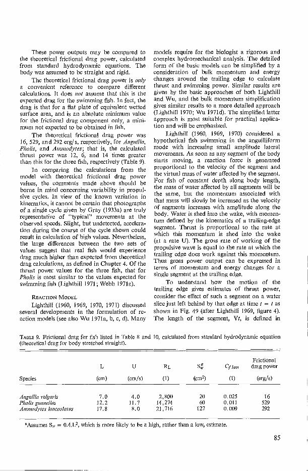
RL

(1) (cm 2) (cm) Species (cm/s)

20 60

127

0.025 0.011 0.009

16 529 292

4.0 11.7 8.0

7.0 12.2 17.8

2,800 14,274 21,716

These power outputs may be compared to the theoretical frictional drag power, calculated from standard hydrodynamic equations. The body was assumed to be straight and rigid.

The theoretical frictional drag power is only a convenient reference to compare different calculations. It does not assume that this is the expected drag for the swimming fish. In fact, the drag is that for a fiat plate of equivalent wetted surface area, and is an absolute minimum value for the frictional drag component only, a mini-mum not expected to be obtained in fish.

The theoretical frictional drag power was 16, 529, and 292 erg/ s, respectively, for Anguilla, Pholis, and Ammodytes; that is, the calculated thrust power was 12, 6, and 14 times greater than this for the three fish, respectively (Table 9).

In comparing the calculations from the model with theoretical frictional drag power values, the comments made above should be borne in mind concerning variability in propul-sive cycles. In view of the known variation in kinematics, it cannot be certain that photographs of a single cycle given by Gray (1933a) are truly representative of "typical" movements at the observed speeds. Slight, but undetected, accelera-tion during the course of the cycle shown could result in calculation of high values. Nevertheless, the large differences between the two sets of values suggest that real fish would experience drag much higher than expected from theoretical drag calculations, as defined in Chapter 4. Of the thrust power values for the three fish, that for Pholis is most similar to the values expected for swimming fish (Lighthill 1971; Webb 1971a).

REACTION MODEL Lighthill (1960, 1969, 1970, 1971) discussed

several developments in the formulation of re-action models (see also Wu 1971a, b, c, d). Many

models require for the biologist a rigorous and complex hydromechanical analysis. The detailed form of the basic models can be simplified by a consideration of bulk momentum and energy changes around the trailing edge to calculate thrust and swimming power. Similar results are given by the basic approaches of both Lighthill and Wu, and the bulk momentum simplification gives similar results to a more detailed approach (Lighthill 1970; Wu 1971d). The simplified latter approach is most suitable for practical applica-tion and will be emphasized.

Lighthill (1960, 1969, 1970) considered a hypothetical fish swimming in the anguilliform mode with increasing small amplitude lateral movements. As soon as any segment of the body starts moving, a reaction force is generated proportional to the velocity of the segment and the virtual mass of water affected by the segment. For fish of constant depth along body length, the mass of water affected by all segments will be the same, but the momentum associated with that mass will slowly be increased as the velocity of segments increases with amplitude along the body. Water is shed into the wake, with momen-tum defined by the kinematics of a trailing-edge segment. Thrust is proportional to the rate at which this momentum is shed into the wake (at a rate U). The gross rate of working of the propulsive wave is equal to the rate at which the trailing edge does work against this momentum. Thus gross power output can be expressed in terms of momentum and energy changes for a single segment at the trailing edge.

To understand how the motion of the trailing edge gives estimates of thrust power, consider the effect of such a segment on a water slice just left behind by that edge at time t = t as shown in Fig. 49 (after Lighthill 1969, figure 4). The length of the segment, Vt, is defined in

TABLE 9. Frictional drag for fish listed in Table 8 and (theoretical drag for body stretched straight).

10, calculated from standard hydrodynamic equation

Frictional Cf lam drag power

(1) (erg/s)

Anguilla vulgaris Pholis gunnellus Ammodytes lanceolatus

°Assumes S1 = 0.4.L2, which is more likely to be a high, rather than a low, estimate.

85

Vt

Wt

Fic. 49. A highly simplified diagrammatic representa-tion of movements of a trailing-edge segment attwo instances in a cycle of transverse motion. Forexplanation, see text. (Based on Lighthill 1969)

relation to the speed V at which the propulsivewave is propagated, overtaking the water sliceat that speed. In time t, this segment moves frompositions aat to bbt, with the trailing edgemoving laterally a distance Wt, and forward adistance Ut. The water is pushed laterally asmaller distance ivt, and the momentum gain ismTiv, when mT is the virtual mass, and it, thevelocity at which it is pushed by the motion ofthe segment.

Lighthill showed that w is given by the kine-matic parameters U, V, and W from similartriangles in Fig. 49. Thus

w t _ (V-U)tWt Vt

or

tv = W[(V - U) /V] (60)

Momentum, mTw is shed into the wake at U,and the trailing edge does work against this at W.Thus, the total rate of working, ET, is given by

ET = 111T1V U W (61)

ET contains two components, the energyrequired to overcome the total drag (thrustpower) and wasted energy shed into the wake.The latter is kinetic energy, EK, associated withacceleration of water to tiv. This kinetic energy

associated with iv is thus

EK = If MT 11,2 U (62)

and the thrust power, E, is given by subtraction

E = ET - EK = mT(tiv W U-I iv2 ij) (63)

The virtual mass associated with the lateralmotion of a segment is

77tT =k pic d2

(64)4

when

d = depth of segment, or trailing-edge depth.

k is a constant close to 1 for a variety of fishsections, including various combinations of dorsaland /or ventral median fins. For practical purposesEquation 64 can then be written;

mT = prc d2 /4 (65)

An important effect of forces produced byany lateral motion is the resulting yawing couple.These yawing forces, termed recoil forces(Lighthill 1960) are associated with recoil move-ments of anterior portions of the body, whichcould be associated with large energy losses(Lighthill 1960, 1969, 1970). All segments execut-ing lateral movements are, of course, doing workassociated with recoil forces. The mean timeaverage of these forces in anguilliform propulsionis zero for symmetrical movements, except at thetrailing edge (Lighthill 1970). In anguilliformpropulsion when there tends to be a completepropulsive wavelength, the integral of recoilforces along the body length tends toward zero.Recoil forces cannot completely cancel out whenthe amplitude increases along the body, as theywill similarly increase. This is reflected by themovement of the nose in anguilliform fish, whichhas an amplitude slightly higher than the mini-mum amplitude observed a short distance alongthe body (Fig. 27).

The model discussed above differs from realfish as follows: (1) amplitudes are assumed to besmall, (2) forces of viscous origin are neglected,except in terms of thrust having to overcome adrag component of viscous origin, (3) efficiencyof the caudal propeller is always greater than 0.5.Amp/itude - The amplitude of real fish move-ments is large, rather than small. Lighthill (1971)considered the effects of large amplitude motionfor the subcarangiform mode, and found it hadlittle effect on total power values in comparisonwith those expected for the small amplitude model,

86

The rate of energy loss to the wake was increased by a factor 1 /cos 0, when O was the angle sub-tended by the trailing edge normal to the axis of forward progression of the fish. (Gray (1933a, b,c) and others usually measured angles subtended by the body of the path of a segment relative to the axis of transverse motion. In Chapter 2, the angle subtended by the body and this transverse axis was given as On, related to O as O 90-0B degrees.)

For normal propulsion in the subcarangiform mode, with O about 600, the mean value of cos 0 for a cycle of trailing-edge movement is about 0.85, making 1 /cos 0 about 1.18 (Lighthill 1971). For anguilliform propulsion, Gray (1933a) noted values of O to 70°, in which case 1/ cos 0 would take mean values of about 1.20. In terms of the overall energetics of the propeller system, the factor 1/cos O will only be important at low propulsive (propeller) efficiencies. With efficien-cies of the order 0.75-0.90, the error involved in using the small amplitude model would be about 5%.

Thrust forces of viscous origin (resistive forces) — Resistive thrust forces, as vorticity shed by a segment, increase with time, and the momentum of the water increases gradually above m-rw (Lighthill 1970). Vortex forces add to both the momentum of the water and the wasted kinetic energy. For this added momentum to be useful in generating thrust, it must be cor-related with the trailing-edge motion, as is mrw with W for reaction forces. Lighthill (1970) showed this was not the case, but rather the momentum resulting from viscous forces would be so correlated that negligible addition to thrust would accrue. The kinetic energy involved would still add to energy loss, with concom-mitant reduction in propeller efficiency. There-fore, neglect of these forces is likely to include a relatively small error in the model's estimation of thrust power, but a larger uncertain error in terms of propeller efficiency.

Propeller efficiency — The small amplitude model assumes that caudal propeller mechanical effici-ency will always be greater than 0.5. This follows from Equation 61, 62, 63, for if mechanical propeller efficiency, ri p, is

ET - EK (66) nT ET

then

rip = 1 - 0.5[(V - U) /V], (67)

neglecting forces of viscous origin.

Then, as V U, rip -> 1, whereas when V »U, rb, -› 0.5. Generally, the model applies for values of U /V between 0.7 and 0.9, when rip

will be high. According to Webb (1971b) this is only likely to occur at speeds approaching max-imum cruising speeds and sprint speeds, at least in the subcarangiform mode. In that mode, low cruising speeds are associated with U/ V as low as 0.23. A consideration of probable muscle behavior suggested that np would then be of the order 0.2-0.25. rip increases with swimmingspeed and increasing U/ V, so that optimum conditions for Lighthill's model are approached at higher speeds. Most measurements in the anguilliform, as well as the subcarangiform mode, have been made for U /V below 0.7 (see values for n in Table 8 and Webb 1971b), in which case the re-action model will tend to overestimate efficiency and thrust power.

In summary, the reaction model is expected to give fair estimates of thrust power, if not total power output, for anguilliform propulsion. The small amplitude model has important advantages in the ease with which key kinematic parameters can be measured without resort to thrust co-efficients.

Example —Data from Gray (1933a) for fish swimming in the anguilliform mode, can again be used with the reaction model (Table 10). The trailing-edge lateral velocity can be calculated assuming its motion is simple harmonic, the root mean square value being appropriate for mean power output.

The thrust power output of Anguilla, Pholis, and Ammodytes for reaction forces was 42, 1714, and 1423 erg /s, respectively, or 2.6, 3.2, and 4.9 times the theoretical frictional drag power in each case. These values are likely to be slightly high, but show that swimming drag will be higher than theoretical drag.

Of the two approaches, resistive or reactive, that proposed by Lighthill is preferred. As set out by Lighthill (1969, 1970) it gives a closer representation of swimming kinematics, and con-siders those forces likely to be of greatest im-portance. It also makes no critical assumptions concerning body sectional shape (see Wu 1971b, c), and in fact includes variations in morphology as a factor affecting hydromechanical efficiency (see next section).

MODIFICATIONS IN THE ANGUILLIFORM MODE An important part of Lighthill's (1969,

1970) and Wu's (1971c) analyses of fish propulsion is the hydromechanical interpretation

87

2.6 0.91 0.65

5.4 1.59 1.98

6.9 1.78 2.49

51 9 42

2052 338 1714

1897 474 1423

TABLE 10. Examples of swimming power output of three fish swimming in anguilliform mode, calculated for reaction forces from the model proposed by Lighthill (1969, 1970). Data for kinematics are from Gray (1933a).

Species LU V f AT

(CM) (CM'S) (CM/S) (S) (CM)

Total Kinetic power energy gener- lost to Thrust

W(rms) w d 111T ated wake power

(cm/s) (cm/s) (cm) (g/cm) (erg/s) (erg/s) (erg/s)

Anguilla vulgaris 7.0 4.0 6.2 1.6 2.1 7.5

Pholis gunnellus 12.2 11.7 17.5 2.0 3.7 16.4

Ammodytes lanceolatus 17.8 8.0 16.0 2.0 3.1 13.8

of some aspects of morphological variation among fish. These are summarized in Fig. 50 and Table 11 based on Lighthill (1969, 1970). Modi-fications of fish morphology relations to anguilli-form motion will be discussed, with some modifications applicable more to the subcarangi-form mode when this tends towards the anguilli-form mode.

Lighthill (1969, 1970) noted several morpho-logical types in the anguilliform mode, associated with tapering posterior body portions, and the subdivision of median fins into discrete fins. Tapering of the posterior of the body reduces mechanical efficiency. Work is done proportional to a segments virtual mass (with d2) and its lateral velocity. When depth decreases, the virtual mass is progressively decreased, and, as with the eel, is associated with only small increases in W. Most work is done by more anterior segments, whereas posterior segments contribute little to thrust but may make substantial contributions to frictional drag and wasted energy in the wake. Two grades of body taper are shown in Fig. 50, Lophotes when this is relatively small, and Gas-trostomus when it is large. Some tapering occurs in any case in Clatnydoselachus, Anguilla, and Lampetra (Fig. 50). However, this is of smaller magnitude compared to the length of the body, and is not likely to alter thrust estimates made with the reaction model.

In contrast, discrete median fins can improve hydromechanical efficiency in comparison with continuous median fins. Two types of morphology are involved, when gaps between the fins are small and when they are large. The former ap-pears more characteristic of such fish as gadids in the subcarangiform mode.

The trailing edge of any fin does work the same as the trailing edge of the caudal fin, and a wake is formed downstream. The wake carries that momentum and energy dictated by the trailing-edge motion in the form of a vortex sheet. When the vortex sheet is shed at the trailing edge of an anterior median fin, it may be resorbed at the leading edge of the next posterior fin, providing its depth is at least as great as that of the anterior fin trailing edge. The wake shed by the posterior fin's trailing edge is dictated by that edge's motion, so that no part of the upstream wake anterior to the posterior fin remains. Thus, the kinetic energy of the upstream motion makes negligible contributions to the total energy wast-age (Lighthill 1970; Wu 1971c). A similar inter-action would be expected for vortex sheets shed by tapering body shapes anterior to a large caudal fin.

When the gaps between median fins are small, as in Gadus, the motion of the leading edge of a posterior fin is similar to that of the wake shed by the trailing edge of an immediately anterior fin, as the phase difference in their motions is small. As such, the leading edge of the posterior fin does no net positive work against the incident wake momentum and the wake momentum is cancelled out over a cycle the same as seg-ments of a continuous fin. The flow is mechani-cally similar to that of a continuous fin, and thrust and efficiency as calculated for the caudal fin trailing edge will be the same. A slight reduction in drag occurs because the gaps in the fins reduce the total surface area.

A different situation applies when gaps are large. The vortex sheet may be resorbed the same as small gaps without a large addition to

88

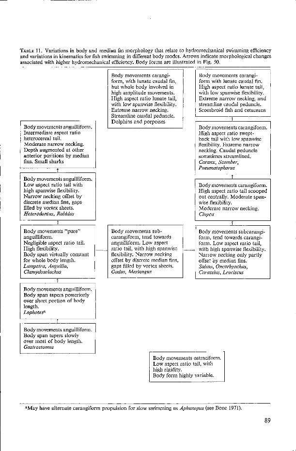
TABLE 11. Variations in body and median fin morphology that relate to hydromechanical swimming efficiencyand variations in kinematics for fish swimming in different body modes. Arrows indicate morphological changesassociated with higher hydromechanical efficiency. Body forms are illustrated in Fig. 50.

Body movements anguilliform.Intermediate aspect ratioheterocercal tail.Moderate narrow necking.Depth augmented at otheranterior posttions by medianfins. Small sharks

i

Body movements anguilliform.Low aspect ratio tail withhigh spanwise flexibility.Narrow necking offset bydiscrete median fins, gapsfilled by vortex sheets.Heterodontus, Rabidus

T

Body movements "pure"anguilliform.Negligible aspect ratio tail.High flexibility.Body span virtually constantfor whole body length.Lampetra, Anguilla,Clamydoselachus

T

Body movements anguilliform.Body span tapers posteriorlyover short portion of bodylength.Lophotesg

T

Body movements anguilliform.Body span tapers slowlyover most of body length.Gastrostomus

Body movements carangi-form, with lunate caudal fin,but whole body involved inhigh amplitude movements.High aspect ratio lunate tail,with low spanwise flexibility.Extreme narrow necking.Streamline caudal peduncle.Dolphins and porpoises

Body movements sub-carangiform, tend towardsanguilliform. Low aspectratio tail, with high spanwiseflexibility. Narrow neckingoffset by discrete median fins,gaps filled by vortex sheets.Gadus, Merlangus

Body movements carangi-form with lunate caudal fin.High aspect ratio lunate tail,with low spanwise flexibility.Extreme narrow necking, andstreamline caudal peduncle.Scombroid fish and cetaceans

T

Body movements carangiform.High aspect ratio swept-back tail with low spanwiseflexibility. Extreme narrownecking. Caudal pedunclesometimes streamlined.Caranx, Scomber,Pneumatophorus

T

Body movements carangiform.High aspect ratio tail scoopedout centrally. Moderate span-wise flexibility.Moderate narrow necking.Clupea

T

Body movements subcarangi-form, tend towards carangi-form. Low aspect ratio tail,with high spanwise flexibility.Narrow necking only partlyoffset by median fins.Salmo, Oncorhynchus,Carassius, Leuciscus

Body movements ostraciform.Low aspect ratio tail, withhigh rigidity.Body form highly variable.

aMay have alternate carangiform propulsion for slow swimming as Aphanopus (see Bone 1971).

89

Squolus °omelets

'Rabidus furiosus

A He le..oen s

frran' eis/cui

Clamydoselochus angu

Lampe/ro

ii Anguilla

rostrato

&wholes

Gaslrostorn

G

L.

0

0 D

Gadus mocrocepholus Oncorhynchus nerka

SUBCARANG IFORM MODE

Kalsuwonas pekes

Bakenop7era borealis

Thunnus saliens

Lcinna di„opis

Pneumatophorus japonicus

Clupea pallasil

CARANGIFORM

MODE

FIG. 50. Diagram illustrating morphological variations that affect mechanical swimming efficiency of fish and cetaceans swimming in various body modes. The important morphological characteristics are given in Table 11.

energy losses. There will now be a large phase difference between the motions of an anterior fin's trailing-edge motion and that of the next posterior fin's leading edge. Lighthill (1970) showed that if the phase difference was greater than 0.5n, the momentum in the upstream wake would not be completely resorbed at the posterior fin's leading edge. Then, there would be a net increase in thrust, without a similar increase in energy losses.

The phase difference between the motion of an anterior fin's trailing edge at a position xi on the body, and the next posterior fin's leading-edge motion at position x2 is given by

Phase difference = 2 It (x2 xi) rv 11 (68) X13 L u

90

when

2 7t (A.2 xl)

gives the phase difference between lateral move-

V ments at xi and x2, and — — 1 modifies this as the

vortex street moves downstream at U with the propulsive wave travelling at V.

This situation probably applies to most sharks, such as Heterodontus and Squall's, and fish like Rabidus when the caudal fin is fully expanded (Fig. 50). For example, Gray (1933a) showed figures of Acanthias vulgaris swimming with U = 17.8 cm/ s, V = 25.6 cm/ s. Length was 46.0 cm, ›.B 30.0 cm. The trailing edge of the

first dorsal fin was about 19.4 cm from the nose, the second dorsal fin was small, so the vortex sheet shed by the first anterior fin would be absorbed at the caudal fin leading edge, at about 37.1 cm. The phase difference between these two is thus, 2n (37.1 — 19.4) (0.44)/30.0 or 0.52n.

In many small sharks there is also a trend to reduction of the body depth posteriorly, with an increase to a high trailing-edge depth at the caudal fin. This is similar to the trend observed in carangiform modes (Fig. 50), except that many elasmobranch body movements are anguilliform. The median fins probably contribute mostly to thrust, rather than to stability as is the case for anterior median fins in the carangiform mode (Lighthill 1970).

Carangiform modes

The hydromechanical theory discussed for anguilliform modes applies to most carangiform modes. An exception is the mode with semilunate tail, and other conditions in the carangiform mode when the caudal fin is highly swept-back, approaching the semilunate condition, (e.g., Pneu-matophorus, Fig. 50). Carangiform modes differ from anguilliform modes in the concentration of significant propulsive movements to the posterior portion of the body (Breder 1926). This applies equally when less than a half wavelength of the propulsive wave is present, as in the carangiform mode proper, and when more than that is present in the subcarangiform variant.

The amplitude of lateral movements increases rapidly over a relatively small portion of the body, compared with a slow rate of increase in the anguilliform mode. According to Lighthill (1970) this is an important hydronnechanical improve-ment, related to the magnitude of resistance thrust forces of viscous origin. In carangiform modes, the time over which these can develop is greatly reduced, and acceleration of water occurs over a short period. The lessening in resistance forces reduces the amount of energy lost to the wake in comparison with the anguilliform mode.

In the anguilliform mode, a trend was noted to greater lateral compression and emphasis on the caudal fin, as in small sharks. This is a domi-nant trend in carangiform modes, when increased thrust comes through increased virtual mass effects at the trailing edge of the body, with increase in that edge's depth.

Although the bulk of thrust will be generated by a caudal fin trailing-edge segment, segments anterior to this trailing edge will also contribute (Wu 1971a, b, c, d). Wu considered in some

detail the effects on thrust of body span (depth) variations between the shoulder and the caudal peduncle particularly as modified by different median fin shapes. Such anterior body section and fin trailing edges will generate a vortex sheet as described above. In the case of anterior fins with sharp trailing edges and a gradually tapering body, thrust enhancement from the motion of segments anterior to the trailing edge is apparently small (Lighthill 1970; Wu 1971c, d). The data discussed below concerns this type of morphology.

When long median fins occur (ribbon-type fins as in the dolphin fish Corphaena hippurus) thrust may be greatly enhanced by the momentum shed by anterior segments (Wu 1971a, b, c, d). Such effects are difficult to include in any analysis, in part because of the complexity of the mathe-matical format and adequacy and feasibility of collecting the necessary data. Problems of in-corporating effects of morphological variation are discussed in Chapter 7.

With the concentration of thrust forces towards the caudal fin, large recoil forces are also generated, no longer balanced by similar lateral forces as with a complete wavelength in the anguilliform mode. Efficient propulsion requires that these forces be minimized, and this is achieved by the characteristic body shape in the carangiform mode. This shape appears from a trend to narrow necking, with body depth progressively reduced in the caudal peduncular region where amplitude increases to its trailing-edge maximum (Lighthill 1969, 1970). It is a trend to the separation of two mass centers; virtual mass effects at the caudal fin as caudal propeller, and the body anterior to the caudal peduncle. Recoil forces generated by the caudal propeller do work against the mass and virtual mass of the body. Where recoil forces act, the body virtual mass is often augmented by a dorsal median fin. Median fins contribute to yawing stability, rather than the generation of thrust. Recoil forces do work against a comparatively greater inertia, effectively minimizing recoil movements. This is clearly shown by the small amplitude movements of the nose of Euthynnus (Fig. 36).

In fish swimming in the subcarangiform mode, narrow necking is poorly developed corn-pared to other carangiform modes. it is often offset by median fins as in Gachts, or anal fins as in salmonids (Fig. 50). In these cases, recoil movements will be less effectively minimized by body shape per se, but it is in these fish that Vestiges of anguilliform motion are retained. The presence of a complete propulsive wave,

91

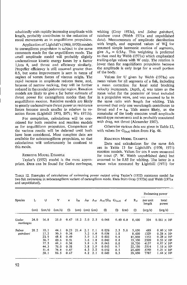
admittedly with rapidly increasing amplitude withlength, probably contributes to the reduction ofrecoil movements as in anguilliform propulsion.

Application of Lighthill's (1969, 1970) modelsto carangiform propulsion is subject to the samecomments made for the anguilliform mode. Thesmall amplitude model will probably slightlyunderestimate kinetic energy losses by a factorI/cos 0, and thrust and efficiency similarly.Propeller efficiency is still assumed greater than0.5, but some improvement is seen in terms ofneglect of vortex forces of viscous origin. Therapid increase in amplitude reduces these, and,because of narrow necking, they will be furtherreduced in the caudal peduncular region. Reactionmodels are likely to give a far better estimate ofthrust power for carangiform modes than foranguilliform motion. Resistive models are likelyto greatly underestimate thrust power as resistanceforces become much smaller in relation to re-action forces (Lighthill 1970, 1971; Wu 1971b).

For completion, calculations will be con-sidered for both resistive and reaction modelsas for anguilliform propulsion. Comparison ofthe various results will be deferred until bothhave been considered. Most complete data areavailable for subcarangiform propulsion, so thatcalculations will unfortunately be confined tothis mode.

RESISTIVE MODEL EXAMPLE

Taylor's (1952) model is the most appro-priate. Data can be found for Gadus inerlangus,

whiting (Gray 1933a), and Salnio gairdneri,rainbow trout (Webb 1971a and unpublisheddata). Measurements of amplitude distributionwith length, and expected values of WÂ forassumed simple harmonic motion of segments,give A,v = 0.5AT. This weighting is preferredto that used by Webb (1971a) which emphasizedtrailing-edge values with W only. The relation islower than for anguilliform propulsion becausethe amplitude is only large for a small portionof the body.

Values for U given by Webb (1971a) aremean values for all segments of a fish, includinga mean correction for local solid blockingvelocity increments. Depth, d, was taken as themean value for the posterior of trout includedin a propulsive wave, and was assumed to be inthe same ratio with length for whiting. Thisassumed that only one wavelength contributes tothrust and != 7,,E. This seems likely, as theremainder of the body executes small amplituderecoil-type movements and is probably associatedwith drag, not thrust (Alexander 1967).

Otherwise various data are given in Table 12,with values for G(,,,,,) taken from Fig. 48.

REACTION MODEL EXAMPLE

Data and calculations for the same fishare in Table 13 for Lighthill's (1970, 1971)reaction models. Values for cos 0 were measuredfor trout (P. W. Webb unpublished data) butassumed to be 0.85 for whiting. The latter is amean value measured by Lighthill (1971) for

TABLE 12. Examples of calculations of swimming power output using Taylor's (1952) resistance model fortwo fish swimming in subcarangiform variant of carangiform mode. Data from Gray (1933a) and Webb (1971aand unpublished).

Swimming power

Species L U V n %n AT Aw Aw/2Xo G(,n,a) d R,( per unit totallength power

(cm) (cm/s) (cm/s) (1) (cm) (cm) (cm) (I) (1) (cm) (1) (erg/s) (erg/s)

Gadus 24.0 16.8 25.0 0.67 18.2 5.0 2.5 0.068 0.60 4.0 8,400 334 0.061 X 105

merlangxs

Sabno 28.2 10.1 44.1 0.23 21.4 2.1 1.1gairdneri 17.2 50.5 0.34 3.2 1.6

23.9 48.8 0.49 3.9 1.530.7 60.6 0.51 3.6 1.837.5 69.3 0.54 3.8 1.944.3 76.0 0.58 3.8 1.951.6 76.8 0.67 4.3 2.258.1 86.5 0.67 4.2 2.1

0.026 2.5 5.0 5,050 489 0.10 X 1050.038 1.8 8,600 1329 0.28 X 1050.035 0.8 11,950 1353 0.28 X 1050.042 0.8 15,350 2520 0.53 X 1050.045 0.8 18,750 4157 0.87 X 1050.045 0.7 22,150 5514 1.16 X 1050.052 0.5 25,600 5760 1.21 X 1050.049 0.5 29,050 7787 1.64 X 105

92

TABLE 13. Examples of calculations of swimming power output using Lighthill's (1969, 1970, 1971) reaction models for three fish swimming in subcarangiform variant of carangiform mode. Data from Gray (1933a), Webb (1971a) and Lighthill (1971). Figures in brackets are approximations.

Total Kinetic energy power generated lost to wake Thrust power

UT V f AT W(rms w d MT COSO (ET) (EH) (E)

(cm) (cm/s) (cm/s) (s) (cm) (cm/s) (cm/s) (cm) (g/cm) (1) (erg/s) (erg/s) (erg/s)

Gadusmerlangus 24.0 16.8 26.4 2.0 5.0 22.2 11.3 (4.8) 18.1 0.85 0.76 x 105 0.23 x 10 5 0.53 x 105

Salmogairdneri 28.2 10.1 44.9 2.1 2.1 9.8 7.8 4.2 13.9 0.88 0.097 x 10 5 0.044 x 10 5 0.063 x 105

15.2 51.4 2.4 3.2 17.1 12.0 4.4 15.2 0.88 0.47 x 105 0.19 x 105 0.28 x 105

21.3 49.2 2.3 3.9 19.9 11.3 4.8 18.1 0.89 0.87 x 105 0.28 x 105 0.59 x 105

27.4 59.9 2.8 3.6 22.4 12.1 5.5 23.8 0.93 1.77 x 105 0.51 x 105 1.26 x 105

33.5 68.5 3.2 3.8 27.0 13.8 5.6 24.6 0.93 3.07 x 105 0.84 x 10 5 2.23 x 10 5

39.6 77.0 3.6 3.8 30.4 14.9 6.0 28.3 0.94 5.08 x 105 1.32 x 105 3.76 x 105

45.7 77.0 3.6 4.3 34.4 14.1 6.1 29.2 0.94 6.47 x 10 5 1.41 x 105 5.06 x 10 5

51.8 85.6 4.0 4.2 37.3 14.5 6.1 29.2 0.93 8.18 x 105 1.71 x 105 6.47 x 105

LeucM= leuciscus 30 48 62 (2.5) (6.7) 37 9 8.7 59 0.85 9.60 x 105 0.96 x 10 5 8.64 x 105

Specks

Frictional drag power

(1) (erg/s)

Cf . turb RL s,,

(cm)2 (1)

311.3 10.1 17.2 23.9 30.7 37.5 44.3 51.6 58.1

Salina gafrdneri 28.2 0.0095 0.0083 0.0078 0.0074 0.0071 0.0069 0.0067 0.0065

2.45 X 104 4.85 X 104

6.74 X 104 8.66X 104

1.06X 105 1.25 X 105 1.46X 105

1.64X 10 5

0.015 X 105 0.066 X 105

0.17 X 105 0.33 X 105 0.58 X 105 0.93 X 105 1.43 X 105 1.98 X 105

Leuciscus from Bainbridge (1963). Trailing-edge depth, d, was measured for trout (P. W. Webb unpublished data) but assumed to be 0.2 L for whiting.

For trout, two values of U are appropriate, one for drag and one for thrust. The value applicable to drag, Ud, is the corrected velocity for interference with the flow in the water tunnel where the fish swam. Interference resulted mainly in local drag increments when the body had substantial local sectional area. Ud was the same as U used with Taylor's (1952) model. The caudal fin trailing-edge segment was of negligible cross-sectional area, so the incident velocity for thrust calculations, UT, will be equal to the free stream velocity, lower than Ud•

In addition to calculations relating to bulk momentum and energy, the model proposed by Lighthill (1971) can be used quasi-statically when the net thrust force is the mean value of instanta-neous forces through a cycle. These give the same results as the bulk momentum approach (Lighthill 1970). The required calculations for the latter analysis have been made by Lighthill (1971) for data on Leuciscus from Bainbridge (1963). Mean values of the calculations are in Table 13. Webb made similar calculations at several low cruising speeds for a single trout (see below).

COMPARISON OF RESULTS FROM MODELS

Results of calculations of thrust power may be compared with theoretical frictional drag as

a reference the same as for the anguilliform mode. A turbulent boundary layer is assumed, as measurements on trout were made in water with an intensity of turbulence greater than 0.03. Outer flow conditions are uncertain for Gadus, but a turbulent boundary layer would be expected with the locomotory movements, roughness at eyes and nares, etc. Leuciscus, swimming in a fish wheel (Bainbridge and Brown 1958), was probably swimming in its own wake to some extent. Results of calculations for theoretical frictional drag power are given in Table 14, and various results for this and thrust power from models compared in Table 15.

Of the results, those for Salmo are of greatest interest, based on means of many observations at different swimming speeds. For these fish the measurements of thrust power calculated from the effects of extra drag loads on the kinematics are also available (Webb 1971a) (Table 15). Compared to theoretical frictional drag power, values from both models are relatively higher for lower swimming speeds, although measured values tend to be a constant multiple of approxi-mately 2.8. Thrust power from the resistive force model decreased from 6.7 to 0.8 times the theoretical frictional drag power from low to higher speeds. Values less than 1 must be con-sidered impossible. High thrust power is asso-ciated with relatively high values of f and V with low U, when Gr(„,„) is low. The thrust power for Gadus is of the same order as Salina at similar RL.

Thrust power values calculated from reaction forces for Salina decreased with speed from

TABLE 14. Frictional drag for fish listed in Table 12 and 13 calculated from standard hydrodynamic equations.

Species (cm) (cm/s)

Gadus inerlangus 24.0 16.8 4.03 X 104 230.4a 0.0086 0.047X 105

Leuciscus leuciscus 30.0 48.0 1.31 X 105 360.0' 0.0067 1.33 X 105

nAssumed S„, ,- -- 0.412.

94

TABLE 15. Summary of swimming power output and requirements from Table 12, 13, 14. Power outputs cal-culated from models by Taylor (1952) and Lighthill (1969, 1970, 1971) and Webb (1971a) are shown as multiplesof the theoretical frictional drag.

Thrust powerTheoretical Thrust power Resistance fromfrictional from Taylor's frictional Lighthill's

Swimming (resistance) thrust (reaction)speed drag power model power model

(cm/s) (erg/s) (erg/s) (erg/s)

Gadus merlangus

16.8 0.047 X 105 0.061 X 105 1.33 0.53 X 105 11.5

(erg/s)

Salmo gairdneri

10.1 0.015 X 105 0.10 X 105 6.7 0.063 X 105 4.2 0.04 2.717.2 0.066 X 105 0.28 X 105 4.2 0.28 X 105 4.2 0.30 4.523.9 0.17 X 105 0.28 X 105 1.6 0.59 X 105 3.5 0.58 3.430.7 0.33 X 105 0.53 X 105 1.6 1.26 X 105 3.8 1.14 3.537.5 0.58 X 105 0.87 X 105 1.5 2.23 X 105 3.8 2.02 3.544.3 0.93 X 105 1.16 X 105 1.2 3.76 X 105 4.0 3.06 3.351.6 1.43 X 105 1.21 X 105 0.8 5.06 X 105 3.5 4.51 3.258.1 1.98 X 105 1.64 X 105 0.8 6.47 X 105 3.3 6.33 3.2

Leuciscus leuciscus

48.0 1.33 X 105 - - 1.01 X 106 7.6 -

4.2 to 3.3 times the theoretical frictional dragpower. This modest decrease can be attributed tochanges in U/V which approach conditions moreappropriate for the model as U increases. Athigher speeds, thrust power from reactive forcesis about 20% higher than that measured byWebb (1971a). This too may be attributed torelatively low U/V, when 7In is likely to beoverestimated. The maximum value for U/Vwas 0.67 for Salmo, but higher values are expectedat higher speeds (Webb 1971b). These higherspeeds will be those more typical of higher cruisingspeeds of most fish, and of sprint speeds.

Differences between the thrust power fromreaction forces and theoretical frictional dragfor Gadus and Leuciscus were 11.5 and 7.6,respectively, much higher than for trout. Thiscould partly be the effects of nonrepresentativesampling in the sequences used in the analysisas for data in the anguilliform mode. A series ofcalculations for a single trout swimming overthe same speed range as those above was madefor the detailed quasi-static approach describedby Lighthill (1971) (P. W. Webb unpublisheddata). This was subject to the same reservations,and gave a mean thrust power 1.3 times the theo-

retical frictional drag power. This indicates apossible range in results based on observationsof single cycles of propulsive activity.

It appears that Lighthill's (1969, 1970, 1971)models will give a reasonable estimate of swim-ming thrust power requirements. This conclusionmust be qualified by two conditions. First, theobvious condition that calculations must bebased on a large number of observations. Thispractically limits general usage to the smallamplitude model, with cos 0 taken into accountas its mean value. Second, the model is mostacceptable at higher cruising speeds and sprintspeeds, speeds greater than 2 L/s.

Carangiform mode with semilunate tail

The carangiform mode with semilunate tailis characteristic of fast swimming fish and ceta-ceans, and probably fish requiring a stablebase line for the lateralis or electrical detectionsystems at low speeds. As details of the locomotionof the latter group are not known, discussion willbe restricted to the former.

The fastest swimming fish and cetaceanshave developed to the greatest extent the various

Reaction Measuredfrictional Thrust frictional

thrust power thrustpower measured power

95

Model thrust

L U f power

(cm) (cin/s) (s) (erg/s)

Theoretical frictional

drag power (erg/s)

Model thrust

power as multiple of frictional

drag power (1)

Species ( 1 )

Cf turb

( 1 )

ça

(cm2)

Delphinus bairdi

Phocoenoides dalli

Lagenorhynchus obliquidens

trends seen in carangiform propulsion. They have a well-defined 'caudal propeller,' the shape of which gives this variant of the carangiform mode its name. The 'propeller' is linked to the body by a narrow caudal peduncle. The caudal peduncle is often streamlined to further reduce flow disturbances anterior to the caudal fin (Slijper 1961; Fierstine and Walters 1968; Magnuson 1970). The body itself tends to be more circular than elliptical (see sections in Carey and Teal 1969a, b). This will be associated with concentration of body mass forward to reduce recoil movements, but with a relative reduction in wetted surface area in comparison with elliptical sections. Body mass is further augmented by virtual mass effects associated with the added depth of median fins.

The restriction of significant propulsion to a caudal propeller of short chord (length) in rela-tion to body length means that the slender body theory discussed for long fish will not apply (Lighthill 1970; Wu 1971b). Instead, a different model must be formulated, based on lifting-wing theory for oscillating aero/hydrofoils. Approaches to thrust power may be resistive and quasi-static (von Holste and Kuchemann 1942; Parry 1949a; Gero 1952) or reactive (Lighthill 1969, 1970). The hydromechanical theory de-manded by propulsion with semilunate tail is far more complex than that for elongate fish. Models are generally in preliminary form, and rigorous development is required. This is hampered by the paucity of data for animals swimming in this mode.

The application of models of carangiform propulsion with semilunate tail is otherwise sim-plified at the present time, for most predict thrust or thrust coefficients based on key kine-matic factors. This short circuits the complex hydromechanics for biological application, and these Will be considered. Details of the mechanics can be found in the references in Table 7.

RESISTANCE (QUASI-STATIC) MODEL

The most suitable model is that developed by Parry (1949a) based on the theory of quasi-static flow around oscillating simple aerofoils, from von Holste and Kuchemann (1942). Parry formulated a genera equation for dolphins and porpoises, whereby t -irust power, E, was

E = 0.0175 L2 u 3 [ (0.3 8uL

0.047] (69)

This considered thrust power proportional to f for a dolphin of given size and speed, assum-ing fixed relations between a, A, and f Insufficient data is available to confirm these assumptions.

Data for L, U, and f can be found in Norris and Prescott (1961) for Pacific common dolphin, Delphinus bairdi, and Dall porpoise, Phocoenoides

and in Lang and Daybell (1963), for Pacific striped porpoise, Lagenorhynchus obhquidens. These data are given in Table 16 with thrust power calculated from Equation 69. Comparing this with theoretical frictional drag power (Table 16) thrust power was 6.3, 9.4, and 16.0 times higher

Table 16. Calculations of swimming power output of three cetaceans from the quasi-static model proposed by Parry (1949a), and a comparison with theoretical frictional drag power. Data from Norris and Prescott (1961) and Lang and Daybell (1963).

170 430 1.8 8.96X 109 7.31 X 106 0.0031 11,560 1.42X 109 6.3

200 430 2.1 1.80 X 10 10 8.60 X 106 0.0030 16,000 1.91 X 10 9 9.4

204 554 3.9 6.18 X 1010 1.13 X 107 0.0028 16,646 3.96 X 109 16.0

aAsSUMeS S i,' =

96

for Delphinus, Phocoenoides, and Lagenorhynchus,respectively. These thrust power values wouldnot be unreasonable for dolphins swimming nearthe surface, when drag power could be increasedup to 5 times (Hertel 1966 and Fig. 7). Data usedwere recorded at or near the surface. Two con-flicting pieces of information must also be con-sidered. In Chapter 2 it was noted that porpoiselocomotion is often associated with high ampli-tude movements involving much of the body.This would be expected to cause prematureseparation and increase drag. On the other hand,the observation made by Stevens (1950) on therelatively undisturbed flow in the wake of aswimming dolphin suggests this does not occur.Obviously more information is required on dol-phin and porpoise propulsion.

REACTION MODEL

Thrust values from Lighthill's (1970) prelim-inary two dimensional model will be discussedfor flow in a perfect fluid (see calculations in Wu1971b). Lighthill's model predicts values for athrust coefficient, CT, related to thrust, ET, by

ET =I P St, WZ CT (70)

when

Sh = projected area of caudal fin hydro-foil.

Total power developed, ET is then

ET=I pSt,WZCTU (71)

whereas thrust power E, is given in relation toiln as

E = ET rlp, (72)CT is related to two metameters of the kine-

matics, frequency parameter and proportionalfeathering, and to the axis about which the planeof the fin rotates (yawing axis).

The frequency parameter is given by

frequency parameter = w c /U (73)

when

co = 2Tc f, the angular velocity for as-sumed simple harmonic motion,

c = chord length

and proportional feathering = amax (74)Wmax

whena max = maximum angle of attack, in

radiansWmax = maximum trailing-edge lateral

velocity

This assumes that amax and Wmax will becorrelated.

The yawing axis appears to be toward thecenter of the caudal fin on the basis of osteologyof scombrid fish (Fierstine and Walters 1968).This will be assumed for fish and cetaceans.Details of the effects of the position of yawingaxis on CT and rlr are given by Lighthill (1970)and Wu (1971b).

Lighthill (1970) produced diagrams relatingCT to frequency parameter, for isopleths of equalproportional feathering. An example is in Fig. 51for the yawing axis at the half-chord position.

Few data are available for use with the model.Most complete data for kinematics have beenpublished by Fierstine and Walters (1968) forEuthynnus affinis, but length was not given, andby Lang and Daybell (1963) for Lagenorhynchusobliquidens. CT will be nondimensional, and if

Thrust power p S^l W2 U CT= drag power =} p Sv, U3 CD

dimensional similarity will be maintained, for Shand S,, are proportional to L2, whereas W (withf and A) and U are related to length (Hunter and

Ftc. 51. Relation between thrust coefficient, CT, andfrequency parameter for isopleths of equal propor-tional feathering, 0, for caudal fin in carangiformswimming with semilunate tail. The yawing axis isassumed to be at half chord position. (From Lighthill1969) (Reproduced with permission from Hydro-mechanics of Aquatic Animal Propulsion in AnnualReview of Fluid Mechanics, Vol. 1, p.433; ©AnnualReview Inc. 1968. All rights reserved)

97

TABLE 17. Calculations of swimming power output for two species swimming in carangiform mode with semilunate tail from Lighthill's (1970) preliminary two-dimensional model for motion in a perfect fluid. Data for kinematics are from Lang and Daybell (1963) and Fierstine and Walters (1968).

Species

Thrust power as multiple

Propor- Total of theoretical tional Frequency swimming Thrust frictional

L U f A Wma„ ctmax feathering parameter C. i. W(rms) Sh P power power drag power

(cm) (cm/s) (s) (cm) (cm/s) (rad) (1) (1) (1) (cm/s) (cm2) (1) (erg/s) (erg/s)

Euthynnus 50 155 7.7 10 242 0.52 0.33 0.62 1.1 171 26.8 0.77 0.67 X 108 0.51 X 108 5.7 affinis 190 9.1 286 0.87 0.58 0.60 0.7 202 0.85 0.73 x le 0.62 X 108 3.9

200 10.1 317 0.52 0.33 0.64 1.1 225 0.77 1.49 X 108 1.15 X 108 6.4 235 12.5 393 0.87 0.52 0.67 0.8 278 0.86 1.95 X 108 1.68 X 108 5.9 410 14.5 456 1.05 0.94 0.44 0.3 322 0.92 1.71 X 108 1.57 X 108 1.2

Lagenorhynchus 204 554 3.9 60 735 0.28 0.21 0.40 1.5 520 466 0.77 5.24 X 1010 4.03 x wio 10.2 obliquidens

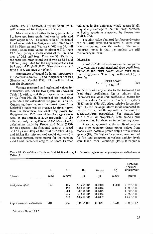
Theoretical frictional

drag power

(erg/s)

RL turb

Species (cm) (cm/s) (1) (1)

50 155 7.75 X 10 5 0.0048 190 9.50 X10 5 0.0046 200 1.00X 106 0.0045 235 1.18 X 106 0.0044 410 2.05 X 106 0.0039

204 554 1.13 X 107 0.0028 16,646

0.89 X 107 1.58 X 107 1.80X 107 2.86X 107 13.4X 107

3.96 X 109

Euthynnus affinis

(cm2)

1 ,000

Lagenorhynchus obliquidens

Zweifel 1971). Therefore, a typical value for L will be assumed for Euthynnus of 50 cm.

Measurements of other factors, particularly Sry, have not been made, but can be estimated from aspect ratio. The aspect ratio of the caudal fin of scombrids like Euthynnus was found to be 6.8 by Fierstine and Walters (1968) (see Nursall 1958a). Span takes values of about 0.27 L (here 13.5 cm), giving a mean chord of 2.0 cm and area of 26.8 cm2 from Equation 37. Similarly, the span and mean chord are shown as 52.1 and 9.0 cm (Lang 1966) for the Lagenorhynehus used by Lang and Daybell (1963). This gives an aspect ratio of 5.8, and area of 466 cm2 .

Amplitudes of caudal fin lateral movements for scombrids are 0.2 L, and independent of size (Hunter and Zweifel 1971). This will be taken here for Euthynnus.

Various measured and estimated values for kinematics, etc., for the two species are shown in Table 17, with lip and thrust power values based on CT from Fig. 51. Theoretical frictional drag power data and calculations are given in Table 18. Comparing these two sets, the thrust power from Lighthill's model was on average 4.6 times higher than the theoretical frictional drag power for Euthynnus and 10.2 times higher for Lagenorhyn-chus. In the former, a large proportion of the difference may be explained on the basis of drag calculations made by Brown and Muir (1970) for this species. The frictional drag at a speed of 1.5 L/ s was 41% of the total theoretical drag, and taking this into account would decrease the difference between thrust power for the reaction model and theoretical drag to 1.8 times. Further

reduction in this difference would accrue if gill drag as a percentage of the total drag increased at higher speeds as suggested by Brown and Muir (1970).

The high value obtained for Lagenorhynehus can be partly explained in terms of extra drag when swimming near the surface. The most important point is that the models are still preliminary in form.

Discussion Results of all calculations can be compared

by calculating a nondimensional drag coefficient, related to the thrust power, which must equal total drag power. This drag coefficient, CD, is given by

thrust power CD - (75)

p S H, U3

and is dimensionally similar to the frictional and dead drag coefficients. CD is higher than theoretical frictional-drag coefficients, except for two low values for resistive forces in Taylor's (1952) model (Fig. 52). Also, resistive forces give high CD for the anguilliform mode compared to reactive forces, but the opposite is the case for subcarangi form propulsion. For carangiform with lunate tail propulsion, both models give similar results, but these are in preliminary form.

A second approach to the results of calcula-tions is to compare thrust power values from models with possible power output from muscle systems (Fig. 53). Values for muscle power output for fish and cetaceans at various activity levels were taken from Bainbridge (1963) (Chapter 6

TABLE 18. Calculations for theoretical frictional drag for Euthynnus affinis and Lagenorhynchus obliquidens in Table 17.

aAssumes S w = 0.4.L2.

99

_1

0U

104 106 10 6 io7 108

REYNOLDS NUMBER - RL

FIG. 52. Relation between drag coefficient, CD, and Reynolds Number, RL. Drag coefficient wascalculated for thrust power values given by hydromechanical models. Open symbols are resistivemodels, closed symbols reaction models, and half closed symbols measured values. Symbols areidentified by generic names. References and further data are given in text, and Table 8, 10, 12, 13, 15,16, and 17. Theoretical frictional drag coefficients are shown as functions of Reynolds Number forlaminar (solid line) and turbulent (broken line) boundary-layer flow.

and Table 19). Making general assumptions thatmass = 0.01 L3 and 0.001 L3 for fusiform andeellike fish, respectively (Bainbridge 1961; Gray1936a), that cruising muscle represents 0.025 bodymass and sprint muscle 0.5 body mass, and qp is0.75, the thrust power output of the muscles can,be estimated. Only half the available muscleworks at any instant.

Most estimates are probably conservative.For example, dogfish myotomes contain 18%0red (cruising) muscle (Bone 1966), rainbow trout17% o (Webb 1970,1971 a), and haddock up to 8%(Fraser et at. 1961). Many fish contain morethan 50% total muscle (Bainbridge 1962). rlp willprobably be greater than 0.75. No direct dataare available for fish muscle power outputs, butfrom Fig. 47 those selected are of the right order.

Thrust power calculated from the variousmodels was within the capacity of estimatedmuscle power output (Fig. 53). It is not certainin most cases if recorded speeds were sprint orcruising speeds. For most carangiform swimmers,including those with semilunate tail, thrust

power was of the order of estimated cruisingmuscle power output. For the anguilliformmode, speeds would probably require sprint andcruise muscle, as would De/phinns and Lngen-orlrynclus, swimming in the carangiform modewith lunate tail. In general, the only difficultyexpected in finding sufficient muscle power tomeet thrust requirements would be for Lagen-orhynchus, should it try to swim much faster thanthe observed 2.5 L/ s. This calculation was basedon a single tail-beat cycle of a porpoise acceler-ating slightly.

The acceptance of any model from compari-sons like those in Fig. 53 involves a tautology,because both thrust power and muscle power areestimates and each has been used to estimate theother. Nevertheless, it indicates that the modelsare "reasonable" and encourages wider use. Muchof the discussion of results from the modelsemphasized inadequacies in the biological datarather than in the models themselves.

It is necessary to summarize recommenda-tions for use of various models. Following

100

1011 r

1010 mammals (sprint))

109

G

10 8 —

• 1• 0 7 —

cr 106 — w

o 0- 10 5 -1 F-

- 1

i 49e0e0 •

_! !

0

10 10-t

cold water fish (sprint) —"

10

< warmwater fish and mammals (cruising)

Zee", -/recks. water fish

o •-• (cruising)

10 4

10 3

10 2

warmwater fish (sprint) I e•

4,49,114:,

102

WEIGHT —g

103 10

4 10

5

FIG. 53. A comparison between thrust power given by various models of fish locomotion, and estimated propulsive muscle power output. Further explanation is given in text. Open symbols are resistive models; closed symbols reaction models, and half-closed symbols measured values.

Lighthill (1970), no truly applicable model for anguilliform propulsion is available. A model combining resistive and reactive approaches is required, which would be difficult to formulate. Otherwise, of the models available, the most suitable is probably that of Lighthill (1960, 1969, 1970) as it makes fewer assumptions than other models and is easiest to apply to real fish data. For carangiform propulsion, excluding the lunate tail variant, the reactive model proposed by Lighthill (1969, 1970) appears most suitable, modified for large amplitude motions after Lighthill (1971). Carangiform propulsion with lunate tail, in preliminary form at present, obviously requires further refinement. Otherwise, Lighthill's (1970) is most suitable for general application (see also Newman 1973; Newman and Wu 1973 ; Wu 1973a, b, c; Wu and Newman 1972).

Acceleration

Introduction

Acceleration, and closely related high-speed maneuver, have been virtually neglected by experimental biologists and hydrodynamicists. Research effort has concentrated on cruising swimming, with the exception of Bainbridge's studies on sprint speeds (1958, 1960, 1962) and occasional reports of acceleration rates (Gero 1952; Gray 1953a; Fierstine and Walters 1968; Hertel 1966; Weihs 1973a). The latter suggested a fairly constant acceleration of the order of 40-50 mis2 for fish ranging from trout to tuna.

Most fish include acceleration phenomena as an integral part of their normal locomotor activity. This is re flected by the muscular system when twitch (fast) muscle typically takes up the larger portion of the axial body-muscle mass

101

(Bone 1966; Love 1970). Acceleration and fast maneuver are essential components of predator approach and /or avoidance behavior, including fishing nets. Clearly this is an area requiring much research.

Kinematics

Weihs (1973a) analyzed qualitatively and quantitatively the mechanics of rapid starting (high speed acceleration) in trout and pike, as an extension of his analysis of high speed maneu-ver (Weihs 1972). Three stages are identified in acceleration.

Preparatory phase —The fish changes its con-figuration from stretched straight to L-shaped by moving the tail laterally so it becomes approxi-mately perpendicular to the body. This takes approximately 0.075 s. Yawing forces are obviously set up by movement of the tail so that the anterior portion of the fish is also rotated about the center of mass.

Propulsive stroke — The caudal fin moves laterally at high speed, subtending a small angle of attack to its direction of motion, and reaching a final position similar to, but the mirror-image of, the original position. The trailing edge moves perpendicularly to the original axis of the fish. The fish initially accelerates at some angle to the original axis because of the rotation of the anterior of the body in the preparatory stage. This takes approximately 0.125 s.

Weihs observed that trout used pectoral fins to return the direction of acceleration to the original axis of the fish. Control of this form will probably be general among fish, as rapid starting is presumably used to reach some objective in minimum time. The propulsive stroke may be repeated several times.

Final phase —Fish behavior is variable in this phase. Fish may continue in a glide with the body stretched straight as in the "nage filée" considered by Houssay (1912) to be the characteristic form of fish swimming. Alternatively, the final stage may be continued swimming in some other pro-pulsion pattern. Unless control movements have been made, the axis of motion in the final phase will continue to subtend some angle to the original axis of the fish.

Weihs also set out a hydromechanical model consistent with the observed kinematics. Numerical solutions gave accelerations in reasonable agreement with observed rates.

Power requirements

An attempt is made to estimate the costs of acceleration for fish of various sizes accelerating at various rates to various final speeds. A sim-plified model will be used, based on thrust /drag predictions for hydromechanical models extrap-olated to accelerating fish on the basis of certain assumptions.

The principal assumptions are that accelera-tion, a, is constant, and that frictional drag at any instant can be calculated from standard hydrodynamic equations

D = p Sw U2 CD (76)

The value CD can be modified to take into account the drag expected for a swimming fish, as predicted by the models discussed above. The ratio between calculated thrust (predicted by application of Lighthill's models to fish) and the frictional drag for an equivalent flat plate was 4.94 for fish swimming in subcarangiform modes. Most data is available for this mode, and accel-eration will be considered for a hypothetical fish, like the trout, swimming in this mode.

Equation 76 can then be rewritten for a swimming fish

D = p S, U2 (4.94 CD) (77)

The boundary layer is most likely to be turbulent so that

D = p S,, U2 [0. 3U) -°.21

(78) v

and grouping constants for a given fish

D = K1 U 1 . 8 (79)

The work done against drag, WD, for uniform acceleration from a speed U0 = 0 to U = U is given by

x

WD -'=" Ki f U 1 ' 8 dx

0

(80)

102

when x is the distance covered in acceleration,given by standard Newtonian mechanics from

Then

U1= Uô -{- 2 a x (81)

WD = Ki J LUô }(2 a x)0.91 dx (82)

o J

Equation 82 gives the work done againsthydrodynamic drag. This is only part of the dragas work is also done in accelerating the fish mass

109

108rn^

wzo

[ FINAL VELOCITY - cm/s

plus added mass. This is the kinetic energy WK,given by

WK = 1.2 M I (U2 - Uô) (83)

when added mass is taken as 0.2 body mass, M.

Then the total work done, W, in acceleratingthe fish is given by

W- Kl ^[U+(2ax)09] dx+

0.6 M (U2 - Uô) (84)

100

250

106

i

^ 7500 4000 2500

10-2

1 i i i iiiil

10 ,

TIME

i i i i i i i I I I I i i i i i

- s

I 10

Fic. 54. Work done in accelerating from rest at various constant rates to various final speeds shownas a function of time to reach final speed. Isopleths are shown for acceleration rates and final speeds.Line AB indicates the limit of expected muscle energy expenditure, the shaded area above this linedelimiting speeds and acceleration combinations outside the capabilities of the hypothetical fish.

103

Ife

be

to'

F› la'

bo°

102 , I

5 6 78 910 20 30 40 50 60 70

LENGTH - cm

The work done in accelerating at various a to various U is shown in Fig. 54 for a hypothetical fish with L = 30 cm, S w = 360 cm2, m = 270 g, and v = 10 -2 poise.

Calculations indicate that the faster a fish accelerates the lower the total energy expended to reach a given speed. This is because the distance covered in reaching a given speed is relatively greater at lower rates or acceleration. Furthermore, the greater the acceleration the shorter the time required to reach a given speed. These two points are of obvious selective advantage.

The isopleths for an acceleration rate of 40 m /s2 and final speed of 300 cm /s are shown by a broken line. These are typical values for a trout of the dimensions used here (Bainbridge 1958; Weihs 1973b), and intersect in the area of the figure when energy expenditure for this acceleration rate approaches minimal values, and the speed is reached in a short time. The time is about 0.1 s, and reasonably similar to that found by Weihs (1973b) for the acceleration propulsion stroke of a trout 33 cm long.

Included in Fig. 54 is an estimate of muscle power expenditure for the fish, calculated simi-larly to values shown in Fig. 53. It assumes an exponential decrease in work done per unit time for the muscle. Fish could reach much higher speeds at the end of acceleration than are gener-ally accepted. Obviously, they could only be maintained for short periods of time. The per-formance of fish for periods of less than a second have not been studied. According to Fig. 54, high speeds would be difficult to attain at low acceleration rates.

The effect of size on work done in accelera-ting at 40111 /s 2 to various specific swimming speeds is shown in Fig. 55. Dimensions are assumed isometric, so that S w = 0.4 L2 and m = 0.01 L3 . The broken line shows the limit of expected muscle energy available. As with other perfor-mance levels, smaller fish are capable of higher specific swimming speeds, although absolute speeds reached would increase with increasing size. Maximum speeds suggested by the calcula-

tions greatly exceed the generally accepted values (10 L /s "rule of thumb"). The cost of reaching a given specific swimming speed also increases with size.

The above model is of course greatly sim-plified. Absolute values for work or time, etc., as shown in Fig. 54, 55 cannot be used without validation. The shape of figures is probably of greatest importance for this will be relatively unchanged by gross errors in any of the assump-tions. The general trend for low costs at high acceleration rates, reaching high speeds in short times, would still be found and the scanty data for fish suggest this is realistic. Ideally, the above figures should be used as the framework in which research may be oriented.

Fin. 55. Work done in accelerating at 40 m /s2 to various final specific swimming speeds shown as a function of length. Broken line indicates limit of expected muscle power output, the shaded area delimiting specific speeds outside the capabilities of hypothetical fish.

104

Summary The main points from Part 1 pertinent to

energetics studies are in Chapter 4 and 5, follow-ing the discussion of hydrodynamics principles and reviews of kinematics and performance. It is concluded (in Chapter 4) that theoretical drag calculations and dead-drag measurements are not valid for the calculation of power require-ments of swimming fish and cetaceans, with a few exceptions. The validity of the rigid-body analogy is denied because movements of swim-ming fish will greatly modify flow with conse-quent substantial drag increments relative to an equivalent rigid body.

Alternative methods of calculating thrust (equal to drag) and power required are explored in Chapter 5. These require the application of hydromechanical models which predict thrust developed by propulsive movements. It is con-cluded that the inviscid models formulated by Lighthill (1960, 1969, 1970, 1971), hereafter referred to as Lighthill's model, are most suitable for application to biological situations at the present time. Predictions of power required in swimming from Lighthill's model agree with the expected muscle power available. These values exceed those for equivalent rigid bodies by 3 to 5 times.

105

_1

PART 2

Chapter 6 - Metabolism and Energy Distribution

Introduction

The propulsive power system of fish can beconsidered as a "black box" with various energyinputs and outputs. Propulsive power output isthe rate of expenditure of only one energy output.In practice, the propulsive system is comprised ofseveral components (Fig. 56). Some may be shown

AEROBICMETABOLICENERGY

Eaaob

PROPULSIVEMUSCLE

HEAT

INPUT TOCAUDAL

PROPELLER

THRUSTET

®

HEAT

FIG. 56. Diagrammatic representation of energy dis-tribution to various components involved in thepropulsion energy system, or "black box," at sustainedswimming speeds. Size of the rectangles representsapproximate distribution proportions of an initial100 units of energy input to the system.

as serial components within which various energytransformations are accomplished in generatingthrust. Other components may be visualized asarranged in parallel (e.g., support systems) andare required for, or are consequences of, contin-uous operation of propulsive muscles. The "blackbox" analogy puts the various components inperspective, and at the same time shows distri-bution and energy flow through the system.

Characterization of the propulsive systemrequires quantification of the various energyinputs and outputs, with the object of relatingthese in terms of conversion efficiencies. Suchefficiencies must be known before locomotoryenergetics may be usefully applied outside lab-oratory situations. This chapter considers themetabolic input to the propulsive system and thedistribution of metabolic energy within that sys-tem, preparatory to a discussion of energeticefficiency in the subsequent chapter.

The question of metabolism is an immensesubject in its own right. Certain aspects have beenextensively studied (e.g., oxygen consumptionrates), others have only recently become amena-ble to research (e.g., energy required in circulat-ing blood), whereas such areas as the precisenature of energy distribution remains largelyspeculative.

This chapter is orientated primarily to non-biologists. Metabolism and energy distributionare not considered in full detail, as discussed inthe introduction to this work.

Production of Biological Energy

Metabolic pathways

Energy is released by a series of chemicalreactions, often referred to as intermediary orcellular metabolism, from one or more basicbody fuels (fat, carbohydrate, and protein). Detailsof these chemical reactions and energy changesare given in standard texts on biochemistry (e.g.,Conn and Stumpf 1963), and have been reviewedby Hochachka (1969) for fish. Only the majorenergetic pathways will be considered.

Two principal energetic pathways may beidentified: (1) aerobic metabolism and (2) anaerobicmetabolism. The former requires oxygen forcomplete oxidation of the fuel, whereas the lattercan progress in the absence of oxygen, involvingincomplete oxidation. Anaerobic metabolism isoften referred to as glycolysis, as the carbohy-drates glucose or glycogen are the most commonsources of energy.

Both pathways generate adenosine triphos-phate (ATP) directly or by coupled reactions. ATPis the immediate cellular source of energy formost biological functions. Hydrolysis of ATPreleases approximately 12 kcal/mol (5 X 1012erg/mol). Fraser et al. (1966) found that codmuscle contained approximately 20 µmol ATP/g,equivalent to 108 erg /g if completely hydrolyzed.

Aerobic and anaerobic pathways generatedifferent amounts of ATP from the same unitpotential energy source. For example, I molof glycogen could generate 38 mol ATP/molglycogen in aerobic metabolism, with carbon

109

dioxide and water as the end products. Glycolysis would generate 3 mol ATP /mol glycogen, with lactic acid as the main end product.

Aerobic metabolism is dependent on the continuous function of cardiovascular and ventilatory support systems for the uptake of oxygen and removal of waste products. The various reactants have high diffusion coefficients in the tissues, and are generated in small amounts in proportion to the energy released. They do not accumulate in the tissues. Aerobic metabolism is the most important metabolic pathway; in normal activity it is generally limited to long-term energy requirements.

Anaerobic metabolism does not depend immediately on physiological support systems, although ultimately aerobic metabolism is re-sponsible for metabolizing lactic acid, either reconstituting it to glycogen or further metab-olizing it to carbon dioxide or water. Anaerobic metabolism can generate large amounts of energy rapidly, to supply demands of short-term bursts of activity. Lactic acid has a relatively low diffusion coefficient in tissues compared to the products of aerobic metabolism, and tends to be accu-mulated. Tissues in the fish propulsion system that function mainly anaerobically (white muscle) require large amounts of energy. As the products of glycolysis tend to be toxic in high enough concentrations, these factors in combination may set a limit to the duration for which glycolysis can operate.

Measurement of Biological Energy

Basic considerations in the measurement of biological energy released by metabolism have been extensively discussed, particularly for domestic animals (Brody 1945; Kleiber 1961); application of these principles to fish have been summarized by Brett (1962, 1973; Krueger et al. 1968; Phillips 1969).

Metabolic energy expenditure of fish is measured by one of two methods : bomb calo-rimetry or indirect calorimetry.

Bomb calorimetry

Metabolic rate of terrestial animals cati be measured from rates of heat production and loss. The most similar method for fish is to measure net caloric (heat) content changes over a given period of time from control samples (at zero time) and exercised experimental samples, each

completely combusted in a calorimeter. This method has not been used in locomotion studies.

Indirect calorimetry Indirect calorimetry is based on calorific

determinations of the heats of combustion of various fuels. Energy released by metabolism is calculated indirectly from the rates at which fuels are used or the rate of oxygen consumed in their combustion. Alternatively energy expendi-ture may be calculated from the rate of produc-tion of such components as carbon dioxide, ammonia, and lactic acid. Indirect calorimetry has been widely applied to locomotion studies and will be considered in some detail.

ENERGY EXPENDITURE FROM BODY FUEL USE

Energy expenditure at any level of activity can be computed from the rate of depletion of body fuels. The three body fuels take heat of combustion values of the order of 9.45 kcal /mol (4.0 X 1011 erg /mol) for a typical fat, 5.65 kcal / mol (2.4 X 10 11 erg /mol) for a typical protein, and 4.1 kcal /mol (1.7 X 10 11 erg /mol) for a typical carbohydrate. Actual values vary to a small extent depending on the particular chemical compounds of fuel used. For fats and carbo-hydrates, the heats of combustion are equal to the total energy liberated by aerobic metabolism, that is, the physiological equivalents are equal to the total physical heats of combustion as the fuels are biologically oxidized to carbon dioxide and water. Proteins contain nitrogen which is transformed and excreted mainly as ammonia (60-70%) and other nitrogenous compounds such as urea and trimethylamine oxide. Proteins are in-completely oxidized in vivo, and the physiological equivalent is lower than the heat of combustion, taking values of the order of 4.8 kcal /g (2.0 X 10 11 erg /g) or 85% of the potential energy (Brody 1945; Kleiber 1961; Brett 1973).

Energy expenditure of sockeye salmon has been computed from fuel depletion at known sustained and prolonged activity levels by Kreuger et al. (1968) and Brett (1973). Total fuel usage of several species of salmon during upstream migra-tion has also been measured (Idler and Clemens 1959; Osborne 1961), but details of performance levels are unknown. Maximum glycogen usage after strenuous activity lias been measured, mainly for salmonids (e.g., Black et al. 1966; Stevens and Black 1966; Wendt 1965, 1967) although not in relation to any defined activity level. Glycogen depletion lias been measured at sustained and prolonged speeds for Gadus morhua

110

by Beamish (1968), and for Carassius carassius by Johnston and Goldspink (1973a, b, c). Variance in glycogen values for control and experimental groups was too high for these data to be used in calculating energy expenditure (Johnston and Goldspink 1973a).

In theory, accurate calculation of energy expenditure from depletion of body fuels requires additional information on particular metabolic pathways. This applies especially to glycogen which is used as the principal fuel for glycolysis (MacLeod et al. 1963; Black et al. 1960; Black et al. 1961; Stevens and Black 1966), as well as being a fuel for aerobic metabolism (Beamish 1968). In practice the relation between metabolic pathways and activity levels is probably suffi-ciently accurate at sustained and burst activity levels that energy contributions from one of the paths may be neglected. For example, at burst activity levels metabolism is mainly anaerobic and contributions from other sources may be neglected as insignificant (Miller et al. 1959; Black et al. 1960; Black et al. 1962; Connor et al. 1964; Beamish 1968).

At intermediate and prolonged activity levels the contribution of various metabolic pathways to the total energy budget is more complex. Gadus morhua and Carassius carassius apparently use glycogen for both aerobic and anaerobic metabolism (Beamish 1968; Johnston and Goldspink 1973a, b, c). Salmonids apparently use glycogen almost exclusively for anaerobic metabolism, and fat and protein for aerobic metabolism (Idler and Clemens 1959; Miller et al. 1959; Black et al. 1960, 1962). The situation for mackerel, Trachurus symmetricus, is also complex (Pritchard et al. 1971). Clearly complete energy budgeting using indirect calorimetry for prolonged speeds would require more complete information on various aspects of metabolic pathways em-ployed and their relative contributions to energy expenditure. It seems probable that such an analysis would lack accuracy, and be sufficiently time-consuming to be of uncertain value. As experimental studies would require sacrificing the fish in any case, it is considered that energy expenditure at these levels could be more profit-ably explored by bomb calorimetry.

OXYGEN CONSUMPTION AND CARBON DIOXIDE PRODUCTION

Oxygen consumption is the most commonly used indirect method of estimating energy expenditure mainly for sustained and prolonged

activity levels (Fry 1971). Calorific equivalents for energy expended when a measured amount of oxygen is respired (oxycalorific equivalents) depend on the fuel being oxidized; equivalents take values of the order of 3.5 cal /mg 02(1.47 X 108 erg /mg 02) for a typical fat, 3.22 cal /mg 02 (1.35 X 108 erg /mg 02) for a typical carbohydrate, and 3.2 cal /mg 02 (1.35 X 108 erg/mg 02) for a typical protein.

These oxycalorific equivalents were initially applied to fish on the basis of comparative physiological equivalents for mammals. Kreuger et al. (1968), in discussing their application to fish, found that the energy expenditure computed from oxygen consumption data was much lower than that computed from fuel consumption based on fat metabolism. This work cast doubt on the application of mammalian derived oxy-calorific equivalents to fish. Brett (1973), in a more detailed study of the question, has shown acceptable agreement betvveen the energy ex-penditure computed from oxygen consumption and that for fuel depletion, allowing for a small amount of error from slight anaerobic metabo-lism. Brett was able to show that the conclusion of large differences made by Kreuger et al. (1968) was based on several false premises.

Measurement of oxygen consumption alone is insufficient to precisely characterize metabolic rate in terms of energy expenditure. Different fuels require differing amounts of oxygen for complete combustion and produce different amounts of carbon dioxide per unit mass metabo-lized. As a result the ratio of carbon dioxide produced to oxygen consumed, or the respiratory quotient, RQ, varies with the three fuels and aids in identifying the fuel used. The RQ takes values of 1.0 for carbohydrate, 0.8 for fats, and 0.7 for proteins. In practice, RQ varies fairly extensively with the chemical species of fuel used, particularly fats when the amount of oxygen consumed depends on the degree of saturation of the molecule. In addition, as all fuels may be used synchronously, RQ values less than 1.0 or greater than 0.7 cannot fully identify the proportions of fuel used. An improvement in the accuracy of using RQ may be achieved if the rate of excretion of nitrogenous materials is also measured. Then the amount of protein metabolized can be estimated separately (Winberg 1956; Brett 1962, 1973; Kutty 1972).

These complicating factors suggest that extremely comprehensive data are required to calculate energy expenditure by means of indirect calorimetry from the proportions of respiratory

111

gases used and excreted. Consequently, in practicea mean oxycalorific equivalent is frequentlytaken; Brett (1973) used 3.36 cal /mg 02 (1.41erg/mg 02) for sockeye salmon, with an assumedRQ of 0.8. The error in using such a mean valuefor the oxycalorific equivalent of oxygen wouldbe approximately 4% if all protein were used.Measurements of RQ for Snlmo gairdneri andTilapia tnossanmbica (Kutty 1968, 1972) at averagesustained swimming speeds, and Carassiusauratus at low sustained speeds (Kutty 1968)gave values between 0.8 and 0.9. Proximateanalysis of the body constituents of migratingsalmon show that mainly fat was used by thefish (Idler and Clemens 1959). These observa-tions indicate that the error in assuming a meanoxycalorific equivalent would be substantiallylower than the 4% maximum. Winberg (1956)considered the use of indirect oxygen calorimetryalone gave an accuracy of ± 1.5% for a normalbody fuel usage.

Use of oxygen consumption measurementsis also subject to a further possible source oferror if some part of the energy budget is madeup by anaerobic metabolism. Anaerobic metabol-ic activity can be detected when the RQ exceeds1.0, i.e., when more carbon dioxide is producedthan oxygen consumed.

Anaerobic energy contributions are usuallymost important at high activity levels (prolongedand burst swimming) and stress conditions(Brett 1962, 1973; Fry 1971; Kutty 1968). Thereare certain exceptions, notably the goldfish(Hochachka and Somero 1971; Smit et al. 1971).This fish can sustain RQ values of between 2and 3 for long periods of time, and operateanaerobically under sustained activity conditions(Kutty 1968). Lactic acid measurements in themuscle used for sustained activity in the tunalikefish Ti•achra•us symmetricus have also shownelevated levels in comparison with those inother fish (Pritchard et al. 1971). This may be aconsequence of the circulatory heat-exchangerin these fish which is designed to conserve heatin the muscles (Barrett and Hester 1964; Careyand Teal 1969a; Carey and Lawson 1973). Thecommonly used increasing velocity test for study-ing power-performance relations for fish usuallyalso neglects anaerobic energy contributions tothe total budget. These are expected at eachspeed increment and at prolonged speeds. Inpractice it is likely that the energy from thissource is small enough to neglect (Webb 1971b).

Oxygen consumption data have been usedto estimate the amount of anaerobic metabolism

that has occurred. Lactic acid metabolismultimately depends on oxygen, so that a periodof strenuous activity is followed by elevatedoxygen consumption levels. As a result an animalaccrues an oxygen debt during that strenuousactivity, which is subsequently paid back.

The use of oxygen debt repayment to measurethe amount of anaerobic metabolism that hasoccurred is not particularly satisfactory. Elevatedoxygen consumption persists for approximately5 h after exhaustion of sockeye salmon (Brett1964) and elevated lactic acid levels persist forapproximately 8 h (Black et al. 1960, 1962),implying poor agreement between the oxygenconsumption and magnitude of the real debt.In addition, some lactic acid may be excreted,although this amount is undoubtedly small(A. J. Mearns personal communication). Ofgreater importance may be lactic acid producedduring recovery, for example as a result of hyper-ventilation required to obtain the additionaloxygen to repay the initial oxygen debt. Factorssuch as these represent sources of substantialerror in estimating anaerobic energy contributionsfrom oxygen debt measurements.

LACTIC ACID PRODUCTION

The amount of lactic acid produced duringburst activity levels represents a possible factorfor an indirect estimate of the energy releasedby glycolysis. Extensive studies of lactic acidproduction have been made mainly by Blackand his collaborators for salmonids and byBeamish (1968) for cod. These studies have beenconcerned with the time course of lactate metabo-lism rather than the relations between specificamounts of lactic acid produced during periodsof activity at known levels, and these data are oflittle use for energetics analysis.

Lactic acid production alone is insufficientto calculate energy released by glycolysis, becauselactic acid is in equilibrium with a second acid,pyruvic acid, at a junction in the metabolicpathways of glycolysis and aerobic metabolism.Pyruvic acid feeds into the aerobic metabolicpathway, and both increased aerobic and anaero-bic metabolism are expected to elevate lacticand pyruvic acid levels. Aerobic metabolismis expected to elevate pyruvic acid levels by anamount similar to lactic acid, whereas anaerobicmetabolism would elevate lactic acid levels farin excess of pyruvic acid levels. Therefore, itwould be necessary to estimate anaerobic energyexpenditure from the amount of lactic acid

112

produced in excess of pyruvic acid (Huckabee1958). Measurements in sufficient detail, and atspecified activity levels, have not been made forfish.

Measurement of energy released by anaerobicmetabolism from lactic acid production usuallyentails sacrificing the fish. Cannulation of thevascular system and serial measurement ofblood lactic acid may be a suitable substitute,but lactic acid appears in the blood over longperiods of time following strenuous activity, soestimates of total production would be difficult.Also, metabolism of lactic acid in situ, excretion,production by hyperventilation, etc., may besufficient to further confound such measurements.

SUMMARY

Indirect calorimetry using oxygen consump-

tion data remains the most valuable method ofmeasuring energy expenditure for most fish atsustained and lower prolonged activity levels.Insufficient data are available to make usefulgeneralizations concerning other methods, ap-plying largely to higher activity levels. Becauseof the usual necessity to sacrifice the fish, andcomplexities of analysis, bomb calorimetry isprobably a more acceptable method of measuringenergy expenditure than indirect methods athigher activity levels.

Metabolic Rates

Aerobic metabolism

OXYGEN CONSUMPTION AND SWIMMING

SPEED

Aerobic metabolic rates are measured interms of oxygen consumption, sometimes sup-plemented by RQ data. Brett (1964) indicatedthat the relation between oxygen consumption,QoZ, and swimming speed typically took theform

Qo2 = a ebU (85)

when a and b are constants. Qoz is commonlymeasured in mg 02/kg per h.

This general relation has been confirmedfor all species studied swimming in body andcaudal fin modes (e.g. Brett and Sutherland1965; Muir et at. 1965; Smit 1965; Hart 1968;Rao 1968; and others; see Fry 1971), and forCymatogaster aggregata swimming in the labri-form mode (P. W. Webb unpublished data).

METABOLIC LEVELS

Various levels of metabolic rates are com-monly defined from the relation between oxygenconsumption and swimming speed. The twoprincipal levels are identified as standard andactive rates, at zero and maximum sustainedswimming speeds respectively. Standard metabolicrate is defined as the rate when the fish is atcomplete rest; it is calculated by extrapolatingthe Qo2-U relation (semilog transformation) to"zero swimming speed." Active metabolic rateis defined as the metabolic rate for maximumsustained activity, although more commonly itis calculated as the metabolic rate at Ucri1. Assuch, the active rate represents maximum oxygenconsumption at some specified prolonged activitylevel (see Chapter 3). The anaerobic contributionto metabolic rate under these circumstances isneglected, but since Qo2 and U,,.;i values aremeasured from swimming periods of the orderof 60 min at each test speed, that is probably nota serious omission (Webb 1971b).

The determined difference between activeand standard rates is the scope for activity (Fry1947). It represents the amount of oxygen (andindirectly the power) available for propulsion, inexcess of that expended in maintaining thesystem.

Metabolic levels between active and standardmetabolism are variously referred to as routineor intermediate rates. The former will be em-ployed. Routine metabolic rates apply to "nor-mal activity without stress" (Brett 1972).

METABOLIC RATES

Magnitudes of metabolic rates are extremelyvariable, depending on environmental factorsand interspecific differences. Effects of environ-mental factors on metabolic rates have recentlybeen reviewed by Fry (1971). In general, factorsthat reduce swimming performance (Chapter 3)also affect metabolic rates by elevating standardmetabolism, and /or reducing active metabolism,or by elevating anaerobic metabolism (Dicksonand Kramer 1971). In each case, scope for activityand swimming performance are invariably re-duced. It is imperative that experimental workshould take these various metabolic responsesinto account so that spurious data are avoided(Brett 1962, 1970).

Interspecific differences in metabolic ratesalso represent a substantial source of variation.Generalizations are difficult to formulate, as toofew species have been studied in sufficient detail.Variations in standard and active rates of four

113

15 20 25

ACCLIMATION TEMPERATURE- C

FIG. 57. Rates of oxygen consumption as a function of temperature for four active fish. Active and standard metabolic rates are upper and lower lines for each species respectively. Lethal temperature for each species is the vertical broken lines. (From Brett 1972) (Reproduced with permission of North Holland Publishing Co., Amsterdam, Holland)

common species are shown in Fig. 57 as a func-tion of temperature, probably the most important factor affecting metabolic rates in the presence of adequate oxygen. At a given temperature, active and standard rates may vary between species by a factor of up to 5 times.

All fish in Fig. 57 are active fish. Sluggish fish have not been widely studied, but appear capable of substantially lower metabolic rates (Brett 1972).

It is clear that in using oxygen consumption data to calculate energy expenditure, consump-tion rates should be measured directly for the particular experimental conditions. Furthermore, in energetics studies, oxygen consumption data and hydrodynamic data from different sources should be used with caution (Chapter 7).

Anaerobic metabolism — energy released Anaerobic metabolic rates have not been

measured for fish at specific activity levels. Most studies have measured the total glycolytic activity of fish arbitrarily exercised to exhaustion. Mainly salmonids have been used. By pooling the sal-monid data (Miller et al. 1959; Black et al. 1960; Black et al. 1962; Miller and Miller 1962; Wendt

1965, 1967) it was found that when fish were exercised to exhaustion approximately 0.19 g glycogen /100 g muscle was used, equivalent to 1.59 X 1011 erg/100 g muscle.

The Muscle System

Red and white muscle Functional characteristics rather than struc-

tural characteristics of muscle components of the propulsive system are of greater importance in considering energetics. Axial (myotomal) muscle structures have been discussed by Nursall (1956) and Alexander (1967, 1968, 1969).

The muscle system of fish is mainly com-prised of two functional groups. These are designated red and white muscle because of their characteristic coloration in many fish. The two types are usually found in discrete blocks, as shown for Scyliorhinus in Fig. 58. Red muscle is usually superficial, and forms a relatively small portion of the myotome (Boddeke et al. 1959). Some fish have an intermediate muscle system, either as a thin sheet separating red and white muscle blocks as in Scyliorhinus (Bone 1966) or as scattered fibers anions the white muscle as in

114

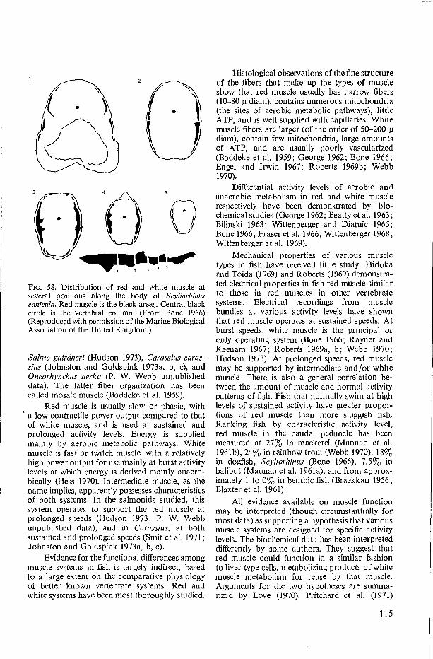
2

C -) u 5

FIG. 58. Distribution of red and white muscle at several positions along the body of Scyliorhinus canicula. Red muscle is the black areas. Central black circle is the vertebral column. (From Bone 1966) (Reproduced with permission of the Marine Biological Association of the United Kingdom.)

Salmo gairdneri (Hudson 1973), Carassius caras-sins (Johnston and Goldspink 1973a, b, c), and Oncorhynchus nerka (P. W. Webb unpublished data). The latter fiber organization has been called mosaic muscle (Boddeke et al. 1959).

Red muscle is usually slow or phasic, with ° a low contractile power output compared to that

of white muscle, and is used at sustained and prolonged activity levels. Energy is supplied mainly by aerobic metabolic pathways. White muscle is fast or twitch muscle with a relatively high power output for use mainly at burst activity levels at which energy is derived mainly anaero-bically (Hess 1970). Intermediate muscle, as the name implies, apparently possesses characteristics of both systems. In the salmonids studied, this system operates to support the red muscle at prolonged speeds (Hudson 1973; P. W. Webb unpublished data), and in Carassitts, at both sustained and prolonged speeds (Smit et al. 1971; Johnston and Goldspink 1973a, b, c).

Evidence for the functional differences among muscle systems in fish is largely indirect, based to a large extent on the comparative physiology of better known vertebrate systems. Red and white systems have been most thoroughly studied.

Histological observations of the fine structure of the fibers that make up the types of muscle show that red muscle usually has narrow fibers (10-80 g diam), contains numerous mitochondria (the sites of aerobic metabolic pathways), little ATP, and is well supplied with capillaries. White muscle fibers are larger (of the order of 50-200 g diam), contain few mitochondria, large amounts of ATP, and are usually poorly vascularized (Boddeke et al. 1959; George 1962; Bone 1966; Engel and Irwin 1967; Roberts 1969b; Webb 1970).

Differential activity levels of aerobic and anaerobic metabolism in red and white muscle respectively have been demonstrated by bio-chemical studies (George 1962; Beatty et al. 1963; Bilinski 1963; Wittenberger and Diatuic 1965; Bone 1966; Fraser et al. 1966; Wittenberger 1968; Wittenberger et al. 1969).

Mechanical properties of various muscle types in fish have received little study. Hidoka and Toida (1969) and Roberts (1969) demonstra-ted electrical properties in fish red muscle similar to those in red muscles in other vertebrate systems. Electrical recordings from muscle bundles at various activity levels have shown that red muscle operates at sustained speeds. At burst speeds, white muscle is the principal or only operating system (Bone 1966; Rayner and Keenam 1967; Roberts 1969a, b; Webb 1970; Hudson 1973). At prolonged speeds, red muscle may be supported by intermediate and /or white muscle. There is also a general correlation be-tween the amount of muscle and normal activity patterns of fish. Fish that normally swim at high levels of sustained activity have greater propor-tions of red muscle than more sluggish fish. Ranking fish by characteristic activity level, red muscle in the caudal peduncle has been measured at 27% in mackerel (Mannan et al. 1961b), 24% in rainbow trout (Webb 1970), 18% in dogfish, *Scyllorhinus (Bone 1966), 7.5% in halibut (Mannan et al. 1961a), and from approx-imately 1 to 0% in benthic fish (Braekkan 1956; Blaxter et al. 1961).

All evidence available on muscle function may be interpreted (though circumstantially for most data) as supporting a hypothesis that various muscle systems are designed for specific activity levels. The biochemical data has been interpreted differently by some authors. They suggest that red muscle could function in a similar fashion to liver-type cells, metabolizing products of white muscle metabolism for reuse by that muscle. Arguments for the two hypotheses are summa-rized by Love (1970). Pritchard et al. (1971)

115

Cold-water fish Warmwater fish Thermo-conserving

fish Mammals

8 x 105 30 x 105 40 x 105

8 x 105 40 x 105

2 x 105 8 x 105 8 x 105

suggested that the red muscle of Trachurus could function in an analagous fashion to the liver at high swimming speeds in addition to its normal muscular activities at lower speeds. In general, it appears that the "liver" hypothesis is supported by few data, whereas that for mechanically different functional systems is comparatively well supported by all data, and is least open to speculation.

Although most fish show well-demarcated red and white muscle blocks, this is not always the case. For example, the myotomal muscle of Anguilla appears to be superficially white, but must function as red muscle to complete the long migrations made by these fish (Boddeke et al. 1959). Structural and functional variations also occur. Red fin muscle in Hippocampus is functionally a twitch muscle (Bergman 1964), comparable to the red, fast, flight muscle in hummingbirds (Aulie and Enger 1969; Grinyer and George 1969). Details of intermediate muscle function remain vague. The extent of such diverse functions contributes to the diffi-culties of interpreting swimming energetics data (Smit et al. 1971).

Muscle power output

At present, no measurements of fish muscle power output have been made. For practical purposes it is assumed that fish muscle is typical of most vertebrate muscle, and that muscle power outputs are comparable on the basis of comparative physiology. Assumed fish muscle power values are usually taken from Bainbridge (1961). Power outputs currently used for fish and cetacean muscle are summarized in Table 19.

TABLE 19. Values for maximum muscle power output assumed for various fish and cetacean muscles (based on Bainbridge 1961).

Muscle power output (erg/s/g)

Red muscle (slow,

nontwitch)

Many problems introduced by "Grays' Paradox" and the use of rigid body analogies to estimate swimming drag are probably related to the use of muscle power values not appropriate for the activity level in question. For example, Gray (1936b) computed muscle power output values for a swimming dolphin on the basis of the unit rate estimated for an Olympic rowing crew working for a 20-min period, that is, probably prolonged activity. The dolphin was undoubtedly swimming at a burst activity level (probably sprint level) when a different muscle system would operate, capable of developing substantially higher power outputs. The rowing crew was certainly using mainly "slow" muscle whereas the dolphin was probably using "fast" muscle.

Power output and muscle shortening speed

Power output of a muscle is not constant but depends on the load and speed of contrac-tion or shortening speed, U„,. Studies by Hill (1950) (see Alexander 1968; Gray 1968) have shown that maximum power is developed when a muscle contracts against a maximum load at a shortening speed of approximately 33% of the maximum shortening speed U„, max, (attained with zero load, Fig. 59). Power outputs remain

100

E 80 a g

so

ià 40

ô 20

2g

10

É-1-i 5 White muscle (fast,

twitch) 100 20 40 60 BO

SHORTENING SPEED — %max

59. Relations between muscle power input, out-put, and efficiency as functions of muscle shortening speed, expressed in relation to maximum power, efficiency, and shortening speeds. (Redrawn from Hill (1950) from Science Progress, Vol. 38; used with permission of Blackwell Scientific Publications.)

116

10 20 30 40 50 60 SWIMMING SPEED-cm/s

90 80 70

close to this maximum over a speed range from approximately 20 to 40% Um max, decreasing rapidly outside that range. Generally, muscle contracts at a specific speed against a particular load, developing a fixed power.

Maximum efficiency is obtained at approx-imately 20% Um max, and the relation between efficiency and shortening speed is such that efficiency remains fairly close to this maximum over a range of approximately 15-25% Um ... Efficiency decreases rapidly outside this range of shortening speeds. Maximum power and efficiency show reasonable correspondence.

Alexander (1969) suggested that different muscles are designed to operate either at maxi-mum efficiency or maximum power output under normal operational conditions. Red muscle would be expected to operate normally at opti-mum efficiency, as its most likely function is continual working at minimal energetic costs. White muscle is required for burst activity, frequently elicited in response to some threat or attack stimulus. The requirement for this muscle would be to develop maximum power output.

Energy Distribution in the Propulsive System

Anaerobic metabolic energy

Studies on anaerobic metabolism in fish indicate that any energy release will be dis-tributed solely to the propulsive muscles. Stren-uous activity results in a rapid decrease in muscle glycogen and a concomitant rise in lactic acid levels, followed later by an increase in blood lactic and pyruvic acid levels. It is logical that all available energy should be so distributed to the muscles at high activity levels, with other organ systems being involved after that activity, during recovery.

Aerobic metabolic energy The amount of energy available for locomo-

tion is commonly calculated from the difference between oxygen consumption at a given speed and the standard rate, equal to the metabolic scope at the critical swimming speed when the active rate is reached. Not all energy so calculated is available to the propulsive muscles for locomo-tion, as is implicit in many analyses of propulsion energetics (Brett 1963; Smit 1965; Webb 1971a, b; Smit et al. 1971). This limitation is usually recognized in such studies, for Brett (1963) emphasized that standard rate is the minimum deductable from the total oxygen at any speed.

In practice, part of the energy available is required by other systems as illustrated by the flow diagram in Fig. 56. Branchial muscle requires energy for ventilation and the heart for circulation (Brett 1971). Some energy will also be required in the adjustment of the ion-osmoregulatory system which is perturbed as a result of increased oxygen demand. This occurs because increased oxygen consumption via the gills cannot be achieved without increased exchange of ions and water (Steen 1971; Wood and Randall 1973a, b, c). Essentially the energy expenditure by such systems may be considered an increase in maintenance energy costs, propor-tional to the increase in metabolic rate.

The three principal systems recognized as requiring some portion of the aerobic energy developed to provide for locomotion will be considered separately.

ION-OSMOREGULATION

Energetic costs of ion and water regulation are not well known. Rao (1968) measured differ-ences in oxygen consumption of rainbow trout at various salinities and at different swimming speeds. He assumed that ion-osmoregulatory costs were minimal at a salinity of 7.5 %fl . Using this as a reference point the additional ion-osmoregulation oxygen costs resulting from swim-ming activity may be calculated (Fig. 60). Accord-

FIG. 60. Relation between ion-osmoregulatory costs, expressed as a percentage of metabolic scope, and swimming speed for a 100 g rainbow trout at 15 C

in fresh water. Reference salinity was 7.5%0 . (Data from Rao 1968)

117

ing to these data, ion-osmoregulatory costs in-crease exponentially with speed to reach approx-imately 16.7% of the metabolic scope close toU,r,l. A similar maximum value at a swimmingspeed of 60 cn-i /s for 80 g Tilapia nilotica may becalculated from data in Farmer and Beamish(1969.)

BRANCHIAL PUMP AND VENTILATION

Energetic costs of ventilation have beenreviewed by Randall (1970b) and Jones (1971).Energy expenditure by the branchial pumps hasmost commonly been estimated from meanpressure-flow relations across the gills. Energeticcosts, as oxygen consumption, have been cal-culated either by assuming some efficiency valuefor the system, or by measuring oxygen consump-tion after flow and pressures have been increased,by reducing the oxygen content of the water orincreasing the water carbon dioxide content. Acritique of these methods has been given byAlexander (1967) and Cameron and Cech (1970)who generally concluded that the methods wereunsatisfactory. The latter authors attempted toestimate oxygen consumption by the branchialpump from the amount of muscle involved. Esti-mates of the oxygen cost of the ventilationsystem vary between approximately 2 and 43%of total oxygen consumption measured (allestimates for restrained fish).

The work of ventilation in swimming fish iseven less certain than that for restrained fish,particularly as some part of that work is un-doubtedly performed by the locomotory mus-culature, fluid pressure at the mouth assisting theflow of water across the gills (ram ventilation).Three ventilation patterns may be identifiedamong fish based on the operation of the branchialpump during swimming and the dependence onthe branchial muscles. A classification of ven-tilatory systems of free-swimming (pelagic) fishfollows (Webb 1970):

Obligatory rarn verrtilation - Fish swim contin-uously with mouth open. Branchial apparatusnot used in ventilation. Scombrids. (Hall 1930;Walters 1962; Muir and Kendall 1968; Brownand Muir 1970).

Facultative ram ventilation - Fish swim withmouth open and only use branchial apparatusat rest and low swimming speeds. Triakis senri-fasciata (Hughes 1960a), Remora remora (Muirand Buckley 1967), Oncorlrynclrus nerka (Smithet al. 1967).

Other pelagic fish- Branchial apparatus operatesat all swimming speeds and at rest. Chrpeaharengus, Gadus inerlangus, Onus mustela,Crenilabrus inelops (Hughes 1960a, b); Sahnogairdneri (Stevens and Randall 1967; Webb1971a); Sahno trutta (Sutterlin 1969); Cyinato-gaster aggregata (P. W. Webb unpublished data).

Many scombrids rely exclusively on ramventilation and must swim continuously to obtainoxygen. Ram ventilation is obligatory and thework of ventilation is consequently performed bythe propulsive muscles of the body. The sameapplies to "facultative" ram ventilation whenram ventilation is used mainly or exclusivelywhen swimming, and normal branchial ventila-tion employed at rest.

The situation is uncertain for fish thatcontinue to operate the branchial pump duringlocomotion. It is likely that, although the bran-chial muscles operate continuously, positivepressure at the mouth and negative (venturi)pressure at the opercular slit will greatly assistwater flow through the ventilatory system.Observations on Sahno gairdneri and Cymato-gaster aggregata (Webb 1971a, unpublisheddata) suggested that this is often the case. Am-plitude and frequency of ventilatory movementsshowed no significant increases with increasedswimming speed in Salnro, although oxygen con-sumption increased approximately 8-10 times.In Cymatogaster, ventilation and locomotorymovements (labriform mode) are correlated sothe mouth opens as the fish surges forward duringpectoral fin adduction.

It seems likely that gill ventilation is largelya function of the propulsive muscles duringswimming, at least in pelagic fish. The additionalresistance to water flow becomes an integral partof drag, and ventilatory work is performed by thelocomotory muscles rather than a second (bran-chial) muscle system. If this were generally appli-cable to fish, then almost negligible amounts ofenergy would be distributed to the branchialmuscle system in excess of that included in theenergy of standard metabolism.

Brown and Muir ( 1970) calculated thatobligatory ram ventilation in Katsrrwonis pelamiswould represent 9% of theoretical drag, which isprobably close to gill drag for fish swimmingin the carangiform mode with semilunate tail(Chapter 4). It was suggested, on the basis ofthese calculations, that in neutrally buoyant fishventilation could represent approximately 12%of theoretical drag (approximately 4% of total

118

10 20 30 40 50 60 70 80 90 100

% U crlt

drag). Fish that continue to use the branchial pump during swimming fall into this group. Jones (1971) in a theoretical study computed that ventilation of a salmonid-type fish would require a maximum of 9% of the active rate at the associated level of activity.

In summary, the distribution of energy and the exact requirements of the branchial pump remain somewhat uncertain. A maximum require-ment of the order of 10% of the active rate appears reasonable, distributed to the branchial muscles when they continue to do the bulk of the ventila-tory work. Otherwise, the energy distributed to these muscles may differ little from that at rest. Additional research on this problem is clearly required.

CARDIAC PUMP

The oxygen consumption costs of the heart may be calculated the same as those of the branchial muscles — from pressure-flow relations for blood circulation (Davis 1968; Randall 1970a; Jones 1971), but few data are available. A most useful study by Jones (1971) combines various data available in the formulation of a theoretical model of cardiac oxygen costs at various total oxygen demand levels for a 1000 g salmonid-type fish. Jones estimated that the maximum cardiac oxygen requirements amounted to 11% of the active rate at that level of activity.

PROPULSIVE MUSCULATURE

The balance of gross aerobic metabolic energy is directed to the propulsive musculature. This proportion can be obtained by subtracting energy distributed to other systems from the total energy made available. Jones' (1971 figure 2) analysis of branchial and cardiac muscle requirements may be replotted to show the percentage of metabolic scope for activity distributed to these systems at different swimming speeds (Fig. 61). In converting Jones' figure to swimming speeds, a direct relation was assumed between the logarithm of oxygen consumption and swimming speed shown as % U„it in Fig. 61. Jones' model was based on fish similar to Salmo gairdneri, a fish that continues to operate the branchial pump during swimming. In the absence of conclusive data to the contrary, it was assumed that the branchial pump performed a major portion of the ventilatory work during swimming. Ion-osmoregulatory work was assumed equal to that shown in Fig. 60 for a 100 g rainbow trout. These costs are undoubtedly overestimated for

FIG. 61. A tentative representation of distribution of oxygen made available for propulsion to various parts of the propulsive and support systems. Oxygen made available is shown as a percentage of the metabolic scope for activity as a function of swimming speed, shown as % Ucrit. Total oxygen made available (solid line), and that required by branchial and cardiac systems (broken line), are based on Jones (1971). The difference between these, oxygen made available to the tissues in the absence of ion-osmoregulatory work, is shown by the chain-dashed line. Ion-osmoregulatory costs were taken from Fig. 60 (on a tentative basis) and were subtracted from the total to estimate net oxygen available for the locomotory muscles (dotted line).

the 1000 g fish on which Jones' analysis was based, as Rao (1968) found substantial depen-dence of ion-osmoregulatory work on weight, but unfortunately the data are insufficient to extrapolate to the higher weight with confidence.

Figure 61 summarizes the distribution of aerobic energy, in terms of metabolic scope, to four systems as swimming speed increases. When the branchial and cardiac energy requirements are subtracted from the total aerobic energy available most energy is directed to the propulsive muscles to a swimming speed of approximately 80% C4,1 / . The proportion of energy so directed is substantilly reduced above this swimming speed. Proportional increase in ion-osmoregulatory energetic costs with swimming speed reduces the proportion of energy directed to propulsive mus-cles at all speeds. The sum of ion-osmoregulatory, branchial, and cardiac costs may reduce the proportion of aerobic energy for the propulsive muscles by a maximum of 37% of the metabolic scope. At high activity levels, aerobic metabolic energy is augmented by anaerobic metabolism.

119

Chapter 7 — Propulsion Efficiency

Introduction

To understand propulsion problems, evalua-tion of propulsive system efficiency is funda-mental. In bringing together the hydrodynamics and metabolic energetics discussed in preceding chapters, efficiency studies serve to evaluate various inputs and outputs of the propulsion system. Like an equation these must balance and efficiencies must be biologically sensible as deduced on the basis of the comparative physiol-ogy of similar systems. As such, efficiency studies are an important, although indirect, method of evaluating models used to calculate thrust power. Efficiency studies serve to identify or emphasize key areas requiring further research. Efficiency is probably of greatest importance if models are to be used to calculate propulsive metabolic power requirements in field situations.

Many studies have been made on the effi-ciency of various components of the system, but few consider the behavior of the overall propul-sion system. For example, hydromechanical models are concerned only with caudal propeller efficiency (Lighthill 1970; Wu 1971a, b, c). The extensive review of energetics of Bainbridge (1961) discussed only muscle power to thrust power conversions at all activity levels considered.

At present the overall efficiency of fish propulsion systems is most important. Charac-teristics of system components are often a matter of speculation, at least of uncertainty. Study of the overall efficiency is the first step in charac-terizing the behavior of these components, or indicating the degree of likelihood that current assumptions are valid.

Only overall efficiency will be considered, as deficient areas requiring research are imme-diately obvious. These have been frequently mentioned in preceding chapters and include anaerobic metabolic situations, most nonbody / caudal fin modes and, of course, the behavior of system components. The discussion will be limited to studies of aerobic efficiency, and treated on the basis of the method used to determine drag or thrust power: the theoretical drag, dead drag, measured power, or hydro-

mechanical models. Optimum swimming speeds will be discussed as a special case of efficiency.

Results from efficiency studies concerning the ability of fish to develop metabolic power commensurate with thrust power requirements have caused some controversy. "Gray's Paradox" is an excellent example. Much of this controversy depends on the method used to determine the power required to overcome drag, and also on availability and quality of data. In some cases confounding factors such as the activity of the dual muscle system also make interpretation difficult.

Definitions

Efficiencies may be defined in relation to a flow diagram as shown in Fig. 56. Considering first the propulsive power system alone, the rate of aerobic energy made available (metabolic power) may be written Eaerob. The rate of energy expenditure by the propulsive wave in develop-ing thrust to overcome drag (thrust power) may similarly be written as ET. Then the overall aerobic efficiency, Tlaerob, is given by

llaerob = ET lEaerob

The locomotory muscles develop power at Em . The efficiency of conversion of metabolic to muscle power, Ti,,,, is therefore

EmlEaerob

The muscle power output is also the power input to the "caudal propeller," equal to the total rate of working, E, of the propulsive wave. The mechanical efficiency of the caudal propeller, tip, will be given by

rip = ET/En, = ET/E (88)

If the various efficiencies are written as decimals rather than percentages, it follows from the above equations that

Tberob = Tim X Tlp

(86)

(87)

(89)

121

These equations neglect the metabolic power dissipated by support systems. If the metabolic power required by support systems is ewp, then this portion may be included in equa-tions 86 to 89 by making the energy directed to the propulsive system alone equal to Eaerob — Es„p. Then modified efficiencies taking into account energy distribution to all nonpropulsive components may be calculated, written as

erobi 11 n, and ii,.

Efficiency Studies

Efficiency and theoretical drag Calculations of efficiency from metabolic

power and power required to overcome theoretical drag made by Osborne (1961), Smit (1965), and Smit et al. (1971) for fish swimming in carangi-form modes, and for Cymatogaster aggregata (P. W. Webb unpublished data), swimming in the labriform mode are discussed.

SALMON MIGRATION Osborne (1961) compared the power required

to overcome the theoretical drag of several species of salmon with the power available from their consumption of fuel, during upstream migration along the Columbia River system. The latter was computed from published data on body constituents measured at the beginning and end of migration. Theoretical drag power was calculated for a mean migration speed and con-ditions of turbulent boundary-layer flow. Osborne assumed efficiencies of 30% for muscle, rim , and and 80% for propeller efficiencies, ri p, to compare supply and demand, rather than calculate effi-ciencies themselves. Calculations of metabolic power from fuels and power required to overcome drag, ET, were expected to show reasonable agreement. Such agreement was found for only two of six salmon runs for three species, the remainder showed ET in excess of metabolic power available. The discrepancy reported was relatively small, but as ET would undoubtedly exceed the theoretical drag power, the discrepancy would in fact be greater.

Osborne pointed out that actual swimming speeds of fish during migration are not known, nor is the behavior. Swimming behavior is undoubtedly significant during migration whereby fish can take advantage of low water velocity areas and eddies. Weihs (1974) has shown that burst /glide behavior could decrease energy required by 50%. Fish were assumed to rest for two-thirds of the time for the completion

of migration. A shorter resting period would reduce the required migration speed of the fish, and could materially affect calculated power requirements. A more comprehensive study of fuel usage for Fraser River migrants using improved analytical methods has shown that salmon are capable of consuming more fuel than estimated in the early literature (Idler and Clemens 1959). Such factors would probably give values for power requirements and metabolic power available of the same order of magnitude.

GOLDFISH AT SUSTAINED AND PROLONGED SPEEDS

SMit (1965) and Smit et al. (1971) considered the efficiency of propulsion at sustained and prolonged activity levels of goldfish. Initially, Smit (1965) analyzed oxygen consumption data and power required to overcome theoretical drag the same as Osborne. Overall efficiency, %rob, was assumed to be 28%. He found that the metabolic power available exceeded that required by up to 3.5 times, implying either a higher drag or very low swimming efficiency.

Smit et al. (1971) explored efficiency rela-tions using a variety of experimental designs at several temperatures. Their interpretation led to a relation between riperpb and swimming speed such that rlaerob was proportional to U 1 . 6 . The latter conclusion was based on several assump-tions that probably did not strictly apply to their experiments. Power required to overcome drag was assumed to increase with U2 .6, the mean of that expected for laminar or turbulent boundary-flow conditions. The experiments were performed in a Blazka respirometer where the intensity of turbulence undoubtedly exceeded critical values resulting in a fully turbulent boundary-layer flow. It is expected that power required would increase with U2. 8 .

The conclusion that naerob was related to U1 .6 led to the deduction that metabolic rate increased with U". Smit et al. discussed at some length the relation between metabolic rate and U, and concluded that metabolic rate was related to eUb for their fish, as is typical for all other species studied in sufficient detail so far (Chapter 6). It appears that efficiency relations are not related to U in any simple fashion (see also Kliashtorin 1973).

In addition to these general relations for efficiency and swimming speed, efficiencies calculated reached values up to 100% at higher sustained speeds (to 8.5 L/s). Smit et al. (1971) considered a ri a„„b of 20% to be the maximum

122

consistent with purely aerobic metabolism, and values above this would imply a substantial anaerobic contribution to the total energy budget. No oxygen debt was accrued (Kutty 1968). It was concluded from the data that both red and white muscles were used for sustained swimming, which leads to the conclusion that white muscle in goldfish is almost inexhaustible. This part of Smit et al.'s (1971) work leads to several questions concerning the comparative physiology of fish muscle, and the behavior of goldfish muscle in particular, and suggests some desirable lines of research.

Cymatogaster AT 45-MIN Ucrit

Discussion of swimming efficiency and the-oretical drag will be restricted to the critical swimming speed for simplicity. Theoretical drag was calculated from equations 29, 31, and 33 for a 45-min U„i i of 56.5 cm/s for fish with a mean length of 14.3 cm and measured wetted sur-face area of 90.91 cm2. Power required was 7.52 X 104 erg/s.

Metabolic power was calculated from the difference between the standard and active rate, equal to 76 mg 02/kg h and 663 mg 02/kg h respectively. The mean weight of the fish was 35.55 g. The oxycalorific equivalent was assumed to be 1.4 X 10 8 erg /s. Metabolic power expended was 8.13 X 10 5 erg /s.

From these values for theoretical drag power and metabolic power, n aierob iS 9.2%. This value is low compared to caudal fin propulsion at Uutt. It is likely that the muscles would be working at optimum efficiency at U„i i (Alexander 1969) when muscle efficiency would be approxi-mately 20%. Then the low overall efficiency must result from a low pectoral fin propeller efficiency or, alternatively, the drag of the fish is under-estimated.

Observing movements by Cymatogaster during swimming, Webb (1973b) showed that drag would be augmented as a result of recoil movements, fluttering of inactive fins and gill drag (P. W. Webb unpublished data). Such factors could increase total drag to 1.53 times the theoretical drag. This would then give a value of naerob of 14%, with a propeller efficiency of 70%. The latter value for maximum propeller efficiency is only a little lower than values measured for caudal fin propulsion, although it is substantially lower than optimum (maximum) values deter-mined from models (Lighthill 1970; Wu 1971d).

Drag of swimming fish is likely to exceed theoretical drag with the possible exception of fish that swim holding the body fairly straight

and use independent short paired or caudal fin propulsion (Chapter 4). This does not apparently apply to Cymatogaster swimming under these conditions, using an independent pectoral fin propulsion system.

Efficiency and dead drag

Brett (1963), Webb (1970), and A. J. Mearns et al. (personal communication) compared power requirements to overcome dead drag with meta-bolic power for several species of salmonids. Data from the latter authors, analyzed by the same method as used by Osborne, show reasonable agreement between power required and that available at normal efficiencies.

Brett (1963) measured the drag of yearling sockeye salmon and found that power required exceeded aerobic metabolic power available by a factor up to 2.2 times. Various differences between these data and that of Mearns et al. and Webb can be attributed to difficulties in measuring dead drag as described in Chapter 4 (Webb 1974).

Brett (1963) also computed trends in effi-ciency changes with swimming speed by means of a power ratio;

Power ratio =

Power required to overcome dead drag Aerobic metabolic power available

Power ratio is shown as a function of swim-ming speed in Fig. 62. Brett found that power

25

2.0

2 ?- 1.5

° o a •

0.5

0 0 1 2 3

SPECIFIC SWIMMING SPEED — L/s

Fio. 62. Relation between power ratio and specific swimming speed for yearling sockeye salmon tested at 15 C. (Simplified a,fter Brett 1963, 1965b)

4

123

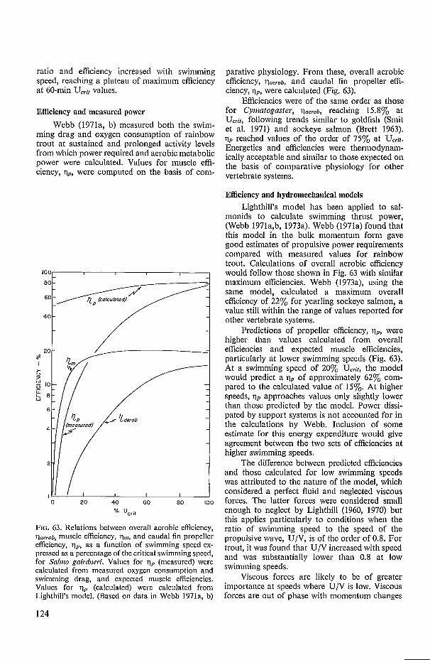
ratio and efficiency increased with swimmingspeed, reaching a plateau of maximum efficiencyat 60-min UC1.;r values.

Efficiency and measured power

Webb (1971a, b) measured both the swim-ming drag and oxygen consumption of rainbowtrout at sustained and prolonged activity levelsfrom which power required and aerobic metabolicpower were calculated. Values for muscle effi-ciency, rlp, were computed on the basis of com-

Fic. 63. Relations between overall aerobic efficiency,

11aerob, muscle efficiency, ri,,,, and caudal fin propellerefficiency, i1p, as a function of swimming speed ex-pressed as a percentage of the critical swimming speed,for Sahno gairdneri. Values for ttr, (measured) werecalculated from measured oxygen consumption andswimming drag, and expected muscle efficiencies.Values for np (calculated) were calculated fromLighthill's model. (Based on data in Webb 1971a, b)

parative physiology. From these, overall aerobicefficiency, llnerob, and caudal fin propeller effi-ciency, np, were calculated (Fig. 63).

Efficiencies were of the same order as thosefor Cymatogaster, ljaerob, reaching 15.8% atU,r;r, following trends similar to goldfish (Smitet al. 1971) and sockeye salmon (Brett 1963).rlp reached values of the order of 75% at Ucrit.Energetics and efficiencies were thermodynam-ically acceptable and similar to those expected onthe basis of comparative physiology for othervertebrate systems.

Efficiency and hydromechanical models

Lighthill's model has been applied to sal-monids to calculate swimming thrust power,(Webb 1971a,b, 1973a). Webb (1971a) found thatthis model in the bulk momentum form gavegood estimates of propulsive power requirementscompared with measured values for rainbowtrout. Calculations of overall aerobic efficiencywould follow those shown in Fig. 63 with similarmaximum efficiencies. Webb (1973a), using thesame model, calculated a maximum overallefficiency of 22% for yearling sockeye salmon, avalue still within the range of values reported forother vertebrate systems.

Predictions of propeller efficiency, np, werehigher than values calculated from overallefficiencies and expected muscle efficiencies,particularly at lower swimming speeds (Fig. 63).At a swimming speed of 20% Uerir, the modelwould predict a nP of approximately 62% com-pared to the calculated value of 15%. At higherspeeds, it, approaches values only slightly lowerthan those predicted by the model. Power dissi-pated by support systems is not accounted for inthe calculations by Webb. Inclusion of someestimate for this energy expenditure would giveagreement between the two sets of efficiencies athigher swimming speeds.

The difference between predicted efficienciesand those calculated for low swimming speedswas attributed to the nature of the model, whichconsidered a perfect fluid and neglected viscousforces. The latter forces were considered smallenough to neglect by Lighthill (1960, 1970) butthis applies particularly to conditions when theratio of swimming speed to the speed of thepropulsive wave, U/V, is of the order of 0.8. Fortrout, it was found that U/V increased with speedand was substantially lower than 0.8 at lowswimming speeds.

Viscous forces are likely to be of greaterimportance at speeds where U/V is low. Viscousforces are out of phase with momentum changes

124

PE

R

KIL

OM

ET

ER

— er

g/k

m

20 30 40 50 60 SWIMMING SPEED — cm/s

_L 10

_L 70 80

and with body movements which do most propulsive work against the inertial forces. As a result, viscous forces add to energy lost in the wake without making significant contributions to thrust (Lighthill 1970). When U/V is small, the time for nonthrust viscous force interactions would be increased, whereas viscous forces developing in magnitude with time (Lighthill 1970) would remain out of phase with body movements and still not contribute to thrust. Webb (1971b) has shown indirectly that rlaerob is related to U/V in the expected fashion.

In general, at low speeds with low U/V, appears to be overestimated by the currently most applicable hydromechanical model. As swimming speed increases so does U/V to reach maximum values of the order of 0.8 as Ucrit is approached, and probably remaining of that order at higher speeds (Webb 1971b). Then Lighthill's model predicts rlp with good accuracy. Lighthill (1969, 1970) indicated the necessity of formulating a model that would sufficiently describe both viscous and inertial forces.

Optimum speed Another approach to the question of effi-

ciency is optimum speed, defined as the speed at which total energy expenditure per unit distance travelled is minimal.

Brett (1965b) has shown that the relation between cost per unit distance and swimming speed has a U-shape (Fig. 64). The initial shape

FIG. 64. Relation between energetic costs (erg /km) and swimming speed of yearling sockeye salmon at three temperatures. Optimum swimming speeds occur at the lowest point of the curve. Predicted optimum speeds (Weihs 1973c) are solid circles. (Based on data in Brett 1964, after Brett 1965b)

of the curve arises because of the inclusion of standard metabolism in total costs; otherwise curves would take a form similar to those shown in Fig. 62, 63. When swimming speed is low, standard metabolic energy costs are high relative to locomotion costs, and the time required to cover unit distance is high. Total costs per unit distance are also high. The situation is further compounded at low speeds as both muscle and propeller efficiencies are low at low speeds. In practice, costs per unit distance are probably overestimated for low swimming speeds as fish are apt to shift to some alternative (more efficient) propulsive mode (e.g., paired fin modes typical of station holding). Such a shift has been observed (Brett and Sutherland 1965; Webb 1971a; Hudson 1973) but has not been rigorously studied, probably because energetics studies become confounded by excitement and restless behavior at low speeds.

Figure 64 shows that the optimum speed shifts and increases with temperature. Energy costs per kilometer also increase with tempera-ture, influenced by the increase in standard or maintenance metabolism, so that it becomes more costly to travel unit distance.

Above the optimum speed, energetic costs per kilometer increase as locomotory costs in-crease with U28 and progressively exceed standard metabolic rate.

Weihs (1973c) derived an expression for optimum speed which predicts that optimum speed would occur when oxygen consumption equals twice the standard rate. These predicted values are included in Fig. 64; they occur some-what lower than the determined optimum speeds. The difference between predicted and determined optimum speeds probably derives from the assumption made by Weihs that naerob increases proportionally with U. icierob is more likely to increase with U raised to some power. Taking this into account would increase the optimum speed predicted by the model, probably approach-ing the observed values as noted by Weihs.

Analysis of Overall Efficiencies

At present Lighthill's model is most suitable for application to bioenergetic studies of fish propulsion. The input parameters may be measured with relative ease for swimming fish. Model predictions of thrust power are within the expected scope of the muscle system. More important than this rather tautological support are the efficiency calculations which show that

125

when sufficient data are available for the calcula-tion of both metabolic and mechanical power expenditures, predictions of thrust power are similar to expected values; in the case of rainbow trout, thrust power calculations show reasonable agreement with measured values. In general, hydromechanical predictions of thrust power are thermodynamically and biologically logical.

The prediction of total power and Tip by the model apparently differs from expected values. This part of the model is of less importance to its full application, as overall efficiencies and indirect calculation of total energy expenditure would likely be of greatest importance in applied situa-tions. The question of tip does require better evaluation.

Hydrodynamic models differ from alter-native methods of calculating thrust-drag power (theoretical and dead drag) as calculations are based on the movements actually made by swimming fish rather than assumptions con-cerning the effects of such movements on drag, which can be shown to be poorly founded in most cases (Chapter 4). Because of the dubious applicability of rigid-body drag calculations, those of hydromechanical models take on a special importance as the only possible alternate method for calculating thrust power with sufficient breadth to be of general predictive value to aquatic vertebrate propulsion problems.

Taking these factors together — the pre-dictive potential of models and their agreement to date with the known physiology and bio-energetics of propulsion system — a more ex-tensive analysis of efficiency based on Lighthill's model is desired.

Such a treatment must be tentative in nature. Agreement between biologically expected and hydromechanically predicted values of thrust power have only been obtained when sufficient data have been available. In contrast, when data from different sources have been equated, dis-crepancies commonly result as with other methods of estimating thrust-drag power.

The major constraint of data availability limits the analysis to salmonids and effects of size. Only one level of activity will be considered, a 60-min Ucrit for sockeye salmon (close to maximum cruising speeds; Brett 1967a). Data are available mainly for metabolic rates of sockeye salmon at 60-min U„i t and, to a lesser extent, the appropriate kinematics (Brett 1964, 1965a, 1967a, and personal communication; Brett and Glass 1973; Webb 1973a, unpublished data). Data are available for kinematics of

rainbow trout in Bainbridge (1958, 1960, 1962, 1963) and Webb (1971a,b).

The model is likely to be most applicable at the activity level selected, when U/V is expected to be high and close to the optimum values.

Lighthill's bulk momentum model, modified for large amplitude motions, will be used. To recapitulate

ET (ter U w W) - mT W2 u /cos 0) (90)

for which the basic input data required are f, A, dT, P, 13, and cos O for any value of Um/

because

W rr f AI -4

w = (f ? - U)/f XB

nIT = 7t ID 3d-

13 will be equal to 1 for the caudal fin trailing edge (Lighthill 1970). Cos O will be assumed equal to 0.85 as measured by Lighthill (1971) for dace, as there are no other measurements.

Kinematics

Data for tail-beat frequency, f, are given by Brett and Glass (1973) and Webb (1973a and unpublished data) for three lengths approximately 5-50 cm. Following the analysis of relations between f, L, and U of Hunter and Zweifel (1971), it was found that

(ff.) 0.339 -I- 0.540 U/L (94)

(R = 0.963)

when fo is the tail-beat frequency at which the regression between f and U/L crosses the U/L axis. fo was found to be related to L by

log fo = 0.799 - 0.474. log L (95)

(R = 0.999)

Values for U„i t are obtained from Brett and Glass (1973) for acclimation and test tem-peratures of 15 C according to the equation

log U„it = 1.129 + 0.634 log L (96)

when Um( is given in cm/s. Numerical values for f and tin* from these equations are in Table 20.

Various values of tail-beat amplitude, A, have been measured for salmonids, mainly for

(91)

(92)

(93)

126

TABLE 20. Basic data for kinematic parameters used to calculate mechanical energy expenditure for sockeyesalmon at the 60-min Ucrit.

Length Ulrit f A

(cm) (cm/s) (s) (cm)

5 37.4 7.31 1.0610 58.0 5.58 2.0115 75.1 4.78 3.0020 90.1 4.39 4.0225 104 3.95 4.9130 116 3.70 5.6440 140 3.32 6.7850 161 3.07 7.6760 181 2.87 8.40

rainbow trout (Table 21). They suggest that A issize dependant, with A/L decreasing withincreasing L (Hunter and Zweifel 1971). As thereare insufficient data for sockeye salmon alone,salmonid values were pooled with the exceptionof an extremely low value of A/L obtained byBainbridge (1958) for a trout 29.3 cm long. Thisvalue for A/L differs markedly from the re-mainder of the data, and it is not certain if it isin fact representative for trout. A curve was fittedby eye to the relation between A and L. Values ofA were then obtained by inspection. No satis-factory linear transformation was found between

TABLE 21. Values for A measured for salmonids.

Species Length A A/L Source(cm) (cm)

Salmo 13.5 2.66 0.197 Bai bridgegairdneri 23.2 4.57 0.197 (1963)

29.3 5.13 0.175 Webb(1971a)

Oncorhyn- 20.4 4.08 0.20 Webbchas nerka (1973a)

51.0 8.00 0.158 J. R. Brett(unpub-lisheddata)

Salmo 29.3 4.016 0.137a Bainbridgegairdneri (1963)

aSee text.

7vD 1D /L dT

(cm) (cm)

7.31 1.46 1.014.85 1.49 2.022.44 1.49 3.030.00 1.50 4.037.50 1.50 5.044.94 1.50 6.060.11 1.50 8.074.92 1.50 10.090.00 1.50 12.0

A and L. Values for A used in calculating ETare included in Table 20.

Estimation of propulsive wavelength, 2,,13,is more difficult. Initially the general relationfor ?,B/L noted by Webb (1971b) and Wu(1971d) was used, but this gave values of ETthat decreased with increasing size, which wouldobviously be unacceptable as inconsistent withboth mechanical and physiological considera-tions. In addition, Webb (1973a) found XB tobe 1.0 for sockeye salmon 20.4 cm long. Itappears that the mean 71B/L obtained by poolingdata from several species swimming in similarmodes (Webb 1971b) is not generally applicable,as differences between species are of sufficientimportance to negate that relation. Samplecalculations using a constant 7,,B/L suggest thisratio will be size dependent, at least for sockeyesalmon.

An alternative method was sought for esti-mating 7vH. On the basis of observations forrainbow trout and several other species swimmingin the same mode, Webb (1971b) noted thatU/f2,B (= U/V) increased with swimming speedto reach values of the order of 0.7 when close tothe 60-min U,r;r. This relation was assumed toapply to sockeye salmon, and ^B calculatedaccordingly (Table 20). Some size dependance ofXB/L is indicated, and all values are greater thanthe value found for one length by Webb (1973a).

No data are available for trailing-edgedepth, dT. dT reaches maximum values at speedsapproaching U,r;r (P. W. Webb unpublisheddata). This is probably general among fish op-timizing swimming efficiency the same as screwpropellers tend to be more efficient with large

127

TABLE 22. Calculated values for mechanical power outputs E, EK, and Sr for sockeye salmon of various sizesat the 60-min U,rij.

Length E

cm (erg/s)

5 2.61 X 10310 3.39 X 10415 1.62 X 10520 5.22 X 10525 1.14 X 10630 2.12 X 10640 5.28 X 10650 1.04 X 10760 1.76 X 107

disc diameters (Chapter 1). Anatomically, dTcould reach 0.2 L for salmon. Values of this orderhave been measured for swimming salmon andtrout, but only for restricted size range(Bainbridge 1963; P. W. Webb un; _ blished data).Therefore, dT will be assumed equal to 0.2 L.

Values for total power, E, power lost in thewake, EK, and thrust power, ET, calculated fromthese data are given in Table 22.

Oxygen consumption

At prolonged swimming speeds, whichinclude the 60-inin U,,;r, most energy is assumedmade available by aerobic pathways and anyanaerobic contribution will be neglected(Chapter 6).

Energy made available for propulsion maybe calculated from the difference betweenactive and standard rates of oxygen consumption,using oxycalorific equivalents. From Brett andGlass (1973) metabolic rates at 15 C are given by

Standard rate = 0.150 M 0•846 (97)(mg 02 /h)

Active rate = 0.951 M 0•963 (98)(Mg 02/11)

These equations require conversion factorsfor weight and length. Weight-length data for 32fish from 5.5 to 18.8 cm, and from 41.8 to 61.4cm in length were given by Brett and Glass (1973).These were supplemented with weight-length datafor 20 fish from 19 to 35 cm long to calculate amore complete weight-length relationship

log M=- 2.180 + 3.089 log L (99)(R = 0.987)

EK ET

(erg/s) (erg/s)

4.60 X 102 2.15 X 1035.98 X 103 2.79 X 1042.85 X 104 1.33 X 10,9.21 X 10, 4.30 X 1052.01 X 105 9.37 X 1053.73 X 10, 1.74 X 1069.31 X 10, 4.35 X 1061.83 X 106 8.55 X 1063.11 X 106 1.45 X 107

Values for weight calculated from Equation 99are included in Table 23, with active and standardmetabolic rates.

The mechanical equivalent of oxygen wastaken as 1.4 X 10$ erg/mgO2. Computed valuesfor metabolic power, E,,eroy are given in Table 24.

Efficiency

Overall efficiency, ilac,•oL, was calculated(Table 24) and is shown as a function of sizein Fig. 65. The relation is curved, with efficiencyincreasing almost logistically with length to reach

TABLE 23. Calculations for weight, standard, andactive metabolic rates for sockeye salmon at the 60-min Ücrit•

Standard Activemetabolic metabolic

Length Weight rate rate(cm) (g) (Gng OZ/h) (mg 02/h)

5 0.95 0.10 0.7510 8.11 0.88 7.1415 23.33 2.54 23.820 68.98 5.39 56.125 137.4 9.66 108.930 241.6 15.6 187.440 587.2 33.0 441.250 1170 59.1 856.760 2055 95.0 1473

128

cm

Length ET

(erg/s)

Eaerob

(erg/s)

%crab

(70)

5 10 15 20 25 30 40 50 60

8.1 10.9 15.3 20.8 24.0 24.8 26.0 26.2 25.8

2.15 X 10 3 2.79 X 104

1.33 X 105 4.30 X 105

9.73 X 105 1.74 X 106

4.35 X 106 8.55 X 106

1.45 X 107

26.7 X 10 3 25.6 X 104

8.69 X 10 5 20.7 X 105 40.5 X 105 7.02X 106

16.7 X 106 32.6 X 106

5.63 X 107

-ynchus nerho-..

•.-Sa/mo goirdneri

60

TABLE 24. Summary of calculations for ET, Eaerob, lberob, for sockeye salmon at the 60-min Ucrit.

EF

FIC

IEN

CY

- %

an asymptote at about 50 cm length. All effi-ciencies are within the range of values anticipated on a comparative physiological basis, but the shape of the curve itself is highly improbable; all efficiencies would be expected to fall within the range of 20-30%.

The shape of the curve, with low efficiencies obtained for small fish, may be explained in one of two ways — either the data or the model are insufficient for the description of the propulsive system. Data for Eaerob are based on extremely comprehensive measurements obtained over many years for large numbers of fish. There is no reason to assume a size dependent variable anaerobic contribution. In contrast, kinematic data are far from complete and solutions to the model can be no better than the input data,

A critical gap exists with respect to kine-matic data. Superficially it appears that the assumptions involved are adequate in obtaining numerical solutions for ET for larger fish (but see below) to which most available data are applicable, although assumptions require vali-dation and, in all probability, correction. Extrap-olation of the data for larger fish to smaller fish is clearly not valid — that is, the assumptions made do not apply throughout the size range considered. This implies that kinematic factors during swimming for sockeye salmon are size-dependent and require further research. Of particular interest is the possibility that kB/L (and dr) varies with size so there could be a change in swimming mode with increasing length. If small fish tended to swim toward the mechan-ically less efficient anguilliform fashion of the subcarangiform mode, and large fish in a more efficient carangiform fashion, then a change in

kinematics with size would be found. In addition, an efficiency-length curve of the form shown in Fig. 65 could be obtained but in a less extreme form.

30

25

20

cai o LCJ

15

101—

1 1 1 1 1 10 20 30 40 50

LENGTH --cm

Fin. 65. Tentative estimates of overall efficiency Ilaerob, as a function of length for sockeye salmon at 15 C. Further explanation is given in the text. Mea-sured values for Oneorhynehus nerka (Webb 1973a) and Salmo gairdneri (Webb 1971b). Shaded area indi-cates range of maximum expected efficiencies.

Another factor that could influence the shape of the curve obtained would be neglect of viscous force effects by the model. At a

129

Length

(cm) (cm2)

RL CT Caerob CD

0.0123 0.0098 0.0086 0.0078 0.0073 0.0069 0.0062 0.0058 0.0055

0.0355 0.0207 0.0136 0.0101 0.0080 0.0068 0.0049 0.0039 0.0032

0.0114 0.0090 0.0083 0.0084 0.0074 0.0067 0.0051 0.0041 0.0033

5 10 15 20 25 30 40 50 60

1.70X 104

5.27 X 104 1.02 X 105

1.64X 105 2.36 X 105 3.16 X 105 5.09 X 105 7.32 X 105

9.87 X 10 5

7.19 31.7 75.5

139.8 225.3 332.8 616.0 993.1

1467.0

length of 5 cm, RL at Ucrit is 1.9 X 104 compared with 1.1 X 10 6 at 60 cm. Although both values are high, the difference may be sufficient to slightly reduce efficiency estimates for small fish.

Thrust and drag

A consideration of thrust and drag reveals further physiological and /or mechanical prob-lems not apparent in the analysis of efficiency alone. The values for ET may be converted to thrust (= drag) coefficients as described in Chapter 5, and compared to theoretical drag coefficients for an equivalent rigid body with turbulent boundary-layer flow. The latter flow conditions are dictateci by the microturbulent nature of flow in the water tunnels used in the experiments. In addition, an expected value for ET may be estimated from data for Eaerob based on the assumption that overall efficiency is 25%. These values for ET can then be expressed as drag coefficients in the same way (Table 25).

The calculations suggest that drag coefficients decrease with size, as expected. Such a phenom-enon could be partially rationalized if swimming mode changes with increasing size.

Comparison between theoretical drag coeffi-cients and those calculated from ET suggest that swimming drag is reduced. Alternatively, if drag were several times theoretical drag as seems more likely, then insufficient aerobic power would be available for fish greater than 30 cm in length as calculation of drag coefficients from Eacrob also gives values less than theoretical drag coefficients. This implies that Gray's

Paradox may apply, but it cannot be assumed that the fish are achieving a much reduced drag; other explanations are possible.

In view of the flow conditions in the water tunnels, and the discussion of drag in Chapter 4, the only likely drag-reducing mechanism appli-cable is mucus, reducing frictional drag in a turbulent boundary layer. Substantial reductions in drag are feasible under time-independent steady flow, but it is not known to what extent drag may be reduced by agents such as mucus in unsteady flow. In general, it seems unlikely that the drag of the swimming fish would be reduced below theoretical drag.

If drag is not reduced, or is reduced by only a small amount, then it must be assumed that more energy is made available to the propulsive system than computed from oxygen consump-tion; that is, the anaerobic energy contribution cannot be neglected for this fish. The problem is analagous to that found by Smit et al. (1971) for goldfish, and they suggested that additional power was made available by the white muscles at higher speeds to supplement the red muscle. The difference between goldfish and salmon problems is one of degree - goldfish can sustain a large anaerobic energy expenditure whereas salmonids cannot (Kutty 1968). Calculation of the possible glycolytic contribution, based on observed maxima discussed in Chapter 6, indicates that adequate energy could be made available to the salmon propulsion system by this means. It may be significant to the solutions of this problem that both cyprinids and salmonids are unusual in having relatively large amounts of intermediate muscle which are electrically active

TABLE 25. A comparison between thrust and drag, expressed as drag coefficients. CT is calculated from data for ET as ET /--p SU3. Ca„,/, is calculated from data for Eaerob assuming ET = 0.25 Enerob CD = (1.2) 0.072 RL-1.

as,,, determined from empirical relationship S = 0.43.L2 . 14 (R = 0.9973; n = 29).

1 30

at the required speeds (Chapter 6). According toWebb's (1970) measurements, intermediate mus-cle could comprise approximately 13% of themyotome. If this muscle is truly intermediate, itwould be necessary to substantially revise effi-ciency criteria at prolonged speeds, such as the60-min U,r;r used here. Questions on energeticsof the intermediate components of the propulsivesystem and division of labor between variousmuscle systems require substantial research, in-cluding comparative studies.

Discussion

Studies of efficiency support the conclusionmade in Chapter 4 that rigid-body analogy isunsuitable for estimating the drag of swimmingfish. Previously, this conclusion was based onhydrodynamic reasons. Here it is based onbiological energetic reasons in that balancedenergy equations are not usually obtained whenthe power required to overcome drag is calculatedfrom theoretical equations or measured for deadfish. In contrast, it was concluded in Chapter 5that Lighthill's model was most suitable forcalculating thrust power, again mainly forhydrodynamic reasons. Comparison betweenmuscle power output and thrust power (Chapter5) and efficiency calculations provide generalbiological support.

Efficiency calculations also support thestatements of several authors of hydromechanicalmodels that present models are not complete. Forexample, caudal fin propeller efficiency appearsto be overestimated by Lighthill's model. Thisprobably stems from the treatment of perfectfluid forces, neglecting viscous thrust and dragforces. Lighthill (1969) clearly pointed to the needfor a composite model, especially for anguilliformpropulsion, to which may be added propulsion ofsmall fish. Lighthill also pointed out that formula-tion of such a model is mathematically problem-atic. Unfortunately it is still not certain thatsuch a "reaction-resistance" model would be ofadditional biological value. Undoubtedly agreater number of parameters and metameterswould be required which may not be amenable toaccurate or actual measurement. It is possible thatsuch a development would return to the situationdescribed by Taylor (1952) when the measure-ment of comprehensive input data would be sotedious and time-consuming, possibly with onlymarginal improvements in quality, as to makesuch a model essentially useless for application. Itmight be of heuristic hydromechanical value only.

Practical application of models does notnecessarily require accurate prediction of pro-

peller efficiency, providing thrust power andoverall efficiency are correctly predicted. Thisintroduces a philosophical difficulty, in that thrustpower is derived from total power and wakepower and np which contains formulation un-certainties. In these terms, it is obvious that notruly satisfactory conclusion can be made.Conceptually the principal problem of viscous'forces is recognized - that is, the mechanicalsystem may be described but the problem remainsof formulating these concepts in an adequatemathematical-hydromechanical framework. In-clusion of viscous forces will tend to lead toincreases in total power and wake power,reducing propeller efficiency but apparently notsubstantially affecting thrust power (Lighthill1969, 1970). The probable exceptions for theanguilliform mode and small fish have beenmentioned.

Although these points do not resolve thephilosophical questions of applying currentmodels, they at least question the biological needor value of more complex, perhaps too complex,models for application, assuming that currentlyapplied models in simpler form are not grosslyfallacious. Questions of this nature must beresolved by the continued development of modelsby hydrodynamicists in working partnership withbiologists. The point concerning input data wasbrought out in the discussion of overall efficienciesof sockeye salmon. In contrast to the conceptualclimate of understanding of the mechanics ofpropulsion by the caudal propeller system, cleardeficiencies are demonstrable in kinematic inputdata. Such data are few, and this is particularlyunfortunate as models cannot be better thaninput data, nor can they be improved and remainaccurate in terms of real fish movements, aspointed out by Breder (1926).

It is legitimate to ask what potential themodels have in applied biology. The principalanswer to this question revolves around estima-tion of locomotory energy requirements ofswimming fish, an expenditure that can representa large proportion of a fish's total energy budget(Brett 1960; Fry 1957, 1971; Kerr 1971a, b, c;Weatherley 1972). Brett (1972) stated: "As yetno one has devised a means for determiningmetabolic rates of fish in nature." Typically,attempts to measure metabolic energy expendi-ture involve the assumption of some relationbetween metabolic rate and weight for someassumed mean routine activity level, a methodwith obvious drawbacks. Brett (1970, 1972)favored the method of measuring time spent atvarious activity levels and applying laboratory

131

determinations of energy requirements to each level, summated for all daily activities to provide a total energy expenditure. This is the method successfully used with higher vertebrates. Brett (1970) discussed this point in greater detail and concluded that extensive research is required in the power-performance area, dividing this into two main areas concerning locomotory mech-anics. Brett called for research in: "1) levels of performance which characterize type activities or behaviour in nature, recorded in such a way that accompanying metabolic costs can be deter-mined by experimentation e.g., tail-beat frequen-cies, distance, and frequency of darts, etc. 2) the development of a means for determining the drag force on swimming fish and hence to evaluate the efficiency of propulsion."

By the use of models in energetics studies it seems likely that a large measure of these objec-tives should be possible. Modern sonar and tagging methods permit measurement of not only speeds and distances covered by fish during their normal activities, but are becoming capable of measuring and transmitting other parameters, for example tail-beat frequencies (Weatherley 1972; Young et al. 1972). Brett (1972) noted that additional parameters such as tail-beat frequency, observable in nature, are desirable, and are "amenable to ascertaining the associated energy demands."

Use of models in estimation of metabolic costs of locomotion is, then, a step further in the direction pointed out by Brett, a method capable of accurate evaluation of mechanical energy expenditure. Parameters such as propulsive wave length may be readily measured in laboratory and (perhaps directly) from field situations. Similarly, relations between trailing-edge depth and speed may be measured in laboratory studies. Tail-beat frequency and amplitude, the principal variants relating speed with thrust power, are observable in the field, as is swimming speed. Variations in cos 0 appear to be small enough that a mean value is acceptable with little loss in accuracy, although this too may be measured in the laboratory. Basic parameters for the measure-ment of thrust for body and caudal fin propulsion should, therefore, present little problem.

Once good measures of thrust power are possible, metabolic costs may be estimated in-directly. For example, it appears that mechanical efficiencies of the propeller system could be empirically related to U/V and/or other specific morphological variations. It also seems likely that muscle efficiencies will not vary signfiicantly from other vertebrate systems, nor between species of

fish, although interspecific differences in the use of various muscle systems may present some problems. Efficiencies of the muscle and propeller system are likely to be related to the same kinematic parameters that provide input data for calculation of thrust power and could facilitate indirect calculation of metabolic energy expenditure.

Such a procedure has a possible advantage with respect to estimating energy expenditure from correlation between swimming speed duration and metabolic rate. Interspecific differences could be accommodated within a semiempirical model, without recourse to detailed measurements of metabolic rates for all species of interest. This does not imply that all fish would have the same locomotory costs (for this is patently untrue), but rather that such variations may be related to specific differences in the efficiencies of the com-ponents making up the propulsive system. Changes in efficiency of these components at different swimming speeds (and between species) could be quantitatively related to kinematic parameters. Such a semiempirical model for fish energetics might be based on simple equations describing swimming kinematics, appropriately "weighted" by suitable coefficients to take into account the effects of morphological and kinematic—energetic variations on thrust and metabolic power. A particularly good example of a semiempirical model to evaluate hovering mechanisms in flying animals was developed by Weis-Fogh (1973).

As a semiempirical model for fish would logically take as its reference point the mechanics of the propulsion system and estimates of thrust power, the nature of the mechanical part should be explored.

The elegant simplicity of the basic bulk-momentum form of Lighthill's model cannot be denied; in fact this is a principal reason the model is suitable for practical application and the reason for emphasis on that model. But this model is neither complete nor definitive. As such, some may argue that the emphasis on one particular model is excessive and this may prove correct. Nevertheless, at present no other model combines the applicability and predictive scope. A positive approach dictates that Lighthill's model should be pursued, but other models, extensions of the same model, and experimental data should be employed to improve its application. In particular the discussion points to changes that would improve a model's prediction of thrust power, and at present this leads to the possibility of a semiempirical model.

132

A positive approach to improving any basic model leads to semiempirical forms at present, because factors neglected in inviscid models are not amenable to simple description in terms of reasonably measurable parameters on swimming fish. Neglect of viscosity is obvious, but D. Weihs (personal communication) developed a mathe-matical expression to explain the effects of viscosity on the inviscid model. Although the resultant expression is not readily amenable to reduction into measurable terms for swimming fish, Weihs was able to indicate the magnitude of the effect of viscosity on virtual mass in terms of modes. Swimming modes themselves are merely verbal descriptions of swimming patterns that may now be expressed in a relatively concise mathematical form, and perhaps ultimately in terms of fish geometry alone. Therefore, the requisite corrections might be numerically ap-proximated in coefficient form as functions of mathematically defined key modal kinematic parameters, and these coefficients in turn could be used to improve the basic model. Also related to mode are the effects on thrust of the rate of increase in amplitude of propulsive move-ments along the length of the body for which Lighthill (1970) developed a mathematical ex-pression. It seems likely that these effects would also be most readily incorporated by suitable coefficients. Similarly, the majority of fish propul-sion models are for slender bodies, neglecting or underestimating the interaction of that vorticity carrying thrust-related momentum with body thickness. This aspect, and the interaction of up-stream trailing vortex sheets with downstream leading edges executing propulsive movements, has been the subject of extensive mathematical research (Lighthill 1970; Wu and Newman 1972; Newman and Wu 1973; Newman 1973). Newman (1973) concluded that such effects would modify Lighthill's (1970) conclusions on forces acting on a swimming fish, but by not more than a maxi-mum of 10%; most fish shapes would involve a negligible correction. Newman pointed out that these effects cannot easily be estimated quantita-

tively for fish-type motions, a situation analogous to that for viscosity, but vortex interaction could be expressed in coefficient form related to fish geometry and kinematics and so applied to the basic model.

Use of the suggested coefficients is not novel to fish propulsion. Lighthill (1970) used such factors to take into account effects of fin and body geometry on virtual mass. Wu (1961, 1971a, b, c), Wu and Newman (1972), Newman and Wu (1973), and Newman (1973) used a coefficient approach to simplify equations for lift and drag of swimming fishes. All models for carangiform propulsion with semilunate tail involve coefficients. In both cases these coeffi-cients are related to fish body geometry and kinematics, computed from solutions to hydro-dynamic equations.

The use of a semiempirical model is an ex-tension of this trend to quantitatively describe factors which cannot be precisely measured. With increased understanding of the propulsive system, the number and variety of coefficients could probably be reduced to a relatively simple multi-factorial equation, or perhaps a simple factor table similar to that obtained by Weis-Fogh (1973) to describe wing geometry of hovering animals. With the probability that a concise and comprehensive hydrodynamic model may be an unreasonable objective, a semiempirical model becomes an attractive alternative, based when possible on good approximations from the more complex aspects of present and future hydro-mechanical models.

The objective of a general semiempirical model to describe fish propulsion is still a con-tinuation of lines of thought already contained in the biological literature discussed (see Brett 1970, 1972; Fry 1971); the development of these lines of thought is largely speculative, but it must be concluded that such a model, coupled with energetics studies, would provide a suitable and more accurate method to determine locomotory costs under natural conditions.

1 33

Summary

Part 2 discussed metabolic aspects of fishpropulsion, and brought them together withhydrodynamics to calculate propulsive efficien-cies. These calculations lead to conclusions similarto those from Part 1, principally that Lighthill'smodel provides a suitable system for calculatingthrust power requirements for a swimming fish.The provisor is made that adequate kinematicdata must be obtained. Efficiency calculationsalso indicate the magnitude of current restrictionsof inviscid models.

The object of formulating a model to predictmetabolic power expended at given swimmingspeeds from kinematic and morphological inputdata is discussed. It is suggested Lighthill's modelwould form a suitable framework and the depthof the model could be increased by means ofsemiempirical coefficients. These could take intoaccount (in coefficient form) factors that presentmeasurement or mathematical problems.

134

Closing Remarks

The most fundamental and difficult problem in fish propulsion studies is the calculation of mechanical thrust (drag) power output. The evolution of the conceptual basis for locomotion studies has largely revolved around this question, a common denominator throughout this work. The question of the drag of swimming fish has been examined from hydrodynamic and metabolic points of view, and it has been found that many approaches to the problem lead to dead ends. It is possible to summarize the main conclusions pertinent to ongoing energetics studies in a few sentences, as in the summaries of Parts 1 and 2. But what has been gained by this dissection of the subject?

The principal conclusion is that hydro-dynamic models provide the best solutions to calculations of thrust power, as the models take as their starting point movements made by swimming fish. Efficiency calculations based on Lighthill's model show that thrust power predic-tions are within a few percent of values that would be predicted from the comparative physiology of propulsion systems, providing complete data are given. This is a marked quantitative improvement over early methods of calculating thrust power from theoretical or dead drag, when discrepancies between hydrodynamic and metabolic estimates of power required differed by up to 5 times for the former, and to several orders of magnitude for dead drag.

The crux of the thrust-power question is not this quantitative improvement. The vital point is the different conceptual basis for calculating thrust power, starting from movements made by swimming fish, rather than on too arbitrary, unsubstantiated assumptions that flow is not seriously disturbed by these movements (rigid-body analogy). This qualitative difference is considered to make such studies as that leading to "Gray's Paradox" irrelevant because the basic premise on which calculations of hydrodynamic

power were made is questioned. The assumptions concerning flow in using the rigid-body analogy are qualitatively different from that on which workable hydrodymanic models are based, because the latter can show that neglect of vis-cosity is likely to have small effect on the flow and mechanics for most fish. Nevertheless, the ques-tion is recognized and is the subject of ongoing research.

In considering the current position of fish en-ergetics studies, problems, pitfalls, and omissions have been continually pointed out, in addition to questions of model application. The major omis-sions must again be emphasized, because under-standing of the gamut of propulsive systems in fish is far from complete. Biological and physical propulsion studies are largely restricted to cruising activity levels for body /caudal fin modes; nonbody /caudal fin modes and low and high (burst, acceleration) activity are identified as the main deficiency areas. It must be emphasized that problems associated with these and other areas are not truly soluble without permanent exchange between physical and biological scien-tists. Discussions in different chapters clearly show why this is necessary.

Finally it will not be amiss to briefly reiterate the objectives of this work. Primarily the intention was to summarize and bring together two ap-proaches to the question of aquatic vertebrate (mainly fish) propulsion energetics with intended mutual benefit. These objectives, with the necessary speculative nature of much of Chapter 7, mean that no attempt has been made to write a definitive treatise; such would be contrary to its intentions, contrary to the definition of research, and would automatically imply stagnation. Given the stated intentions, it is hoped this work will contribute to active, ongoing research by simpli-fying interdisciplinary exchange of ideas. As a result, the only acceptable measure of success will be the rapidity with which this work is outdated.

135

Acknowledgments

In writing this bulletin, I have received the benefit of the experience of my friends and colleagues who willingly gave much of their time to discuss fish locomotion problems with me. They include Dr Q. Bone, Dr J. R. Brett, Dr W. Gosline, Dr M. J. Jarman, Dr T. L. Shaw, Dr G. R. Smith, and Dr D. Weihs. I am particu-larly indebted to those who assisted me by discussing facets in which I have little or no practical experience. I also wish to express my special thanks to Dr Bone for his invaluable support during the course of my doctoral work, some of which is included here for the first time, to Dr Brett and Dr Weihs, who took on the arduous task of reading and criticizing the manu-script and to Natalie Sutterlin for editorial advice. After discussions with various people I frequently modified my ideas, although I doubt they will agree with all I have written. Notwithstanding this debt to my friends, errors remain my responsibility.

The bulk of this work was written during the tenure of a National Research Council of Canada Postdoctorate Fellowship at the Fisheries Re-search Board of Canada, Pacific Biological Station, Nanaimo, B.C., and completed at the

University of Michigan, Ann Arbor, Mich. I am indebted to these organizations for their support.

I would like to thank the following for permission to include reproductions or copies of figures from their publications; Annual Review Inc., Blackwell Scientific Publications Ltd., the Company of Biologists, Dover Publications Inc., the Marine Biological Association of the United Kingdom, McGraw-Hill Inc., North-Holland Publishing Company, The Royal Society of London, the United States Navy, D. Van Nostrand Reinhold Company Inc., and Weidenfeld and Nicolson Ltd. I also wish to thank those authors who allowed me to use their published illustrations, in particular Dr R. Bainbridge, Dr Q. Bone, Dr J. R. Brett, Prof Sir James Gray, and Prof Sir James Lighthill.

I cannot express sufficiently my thanks to my wife, Carol, for her assistance in preparing figures, proofreading, and compiling indices, without whom I could not have completed the bulletin.

Finally I should like to thank Mrs J. Greear for her patience and assistance in typing the manuscript.

136

References

ALEXANDER, R. M. 1967. Functional design in fishes.Hutchinson University Library, London, Eng.160 p.

1968. Animal mechanics. Biology Series.Sidgewick and Jackson, London, Eng. 346 p.

1969. The orientation of muscle fibres in themyotome of fishes. J. Mar. Biol. Assoc. U.K.49: 263-290.

ALEYEV, Y. C., AND O. P. OVCHAROV. 1969. Develop-ment of vortex forming processes and nature ofthe boundary-layer with movements of fish. Zoo].Zh. 48: 781-790.

1971. The role of vortex formation on loco-motion of fish, and the influence of the boundarybetween two media on the flow pattern. Zool.Zh. 50: 228-234.

ALLAN, W. H. 1961. Underwater flow visualizationtechniques. U.S. Nav. Ord. Test Sta. Tech. Publ.2759: 28 p.

AULIE, A., AND P. S. ENGER. 1969. The flight musclesin a bird with high wing-stroke frequency, thezebra finch. Physiol. Zool. 42: 303-310.

BAINI3RIDGE, R. 1958. The speed of swimming of fishas related to size and to the frequency and theamplitude of the tail beat. J. Exp. Biol. 35:109-133.

1960. Speed and stamina in three fish. J.Exp. Biol. 37: 129-153.

1961. Problems of fish locomotion. Symp.Zool. Soc. Lond. 5: 13-32.

1962. Training, speed and stamina in trout.J. Exp. Biol. 39: 537-555.

1963. Caudal fin and body movements in thepropulsion of some fish. J. Exp. Biol. 40: 23-56.

BAINBRIDGE, R., AND R. H. J. BROwN. 1958. Anapparatus for the study of the locomotion offish. J. Exp. Biol. 35: 134-137.

BAMS, R. A. 1967. Differences in performance ofnaturally and artificially propagated sockeyesalmon migrant fry as measured with swimmingand predation tests. J. Fish. Res. Board Can.24: 1117-1153.

BARRETT, I., AND F. J. HESTER. 1964. Body temper-ature of yellowfin and skipjack tuna in relationto sea surface temperature. Nature 203: 96-97.

BEAMISH, F. W. H. 1966. Swimming endurance ofsome northwest Atlantic fishes. J. Fish. Res.Board Can. 23: 341-347.

1968. Glycogen and lactic acid concentra-tions in Atlantic cod (Gadus morhua) in relationto exercise. J. Fish. Res. Board Can. 25:837-851.

BEATTY, C. H., R. D. PETERSON, AND R. M. BOCEK.1963. Metabolism of red and white muscle fibregroups. Am. J. Physiol. 204: 939-942.

BELAYEV, V. V., AND G. V. ZUYEV. 1969. Hydro-dynamic hypothesis of school formation infishes. J. Ichthyol. 9: 578-584.

BELL, W. H., AND L. D. B. TERHUNE. 1970. Watertunnel design for fisheries research. Fish. Res.Board Can. Tech. Rep. 195: 69 p.

BERGMAN, R. A. 1964. The structure of the dorsalfin musculatire of the marine teleost Hippo-campu.s hirrlsonius. Bull. John Hopkins Hosp.114: 344-353.

BILINSKI, E. 1963. Utilization of lipids by fish.(1) Fatty acid oxidation by tissue slices from darkand white muscle of rainbow trout, Salmogairclneri. Can. J. Biochem. Physiol. 41:107-112.

BLACK, E. C. 1957. Alterations in the blood level oflactic acid in certain salmonid fishes followingmuscular activity. 1) Kamloops trout, Salmogairdneri. J. Fish. Res. Board Can. 14: 117-134.

BLACK, E. C., A. R. CONNOR, K. C. LAM, AND W. G.CHIV. 1962. Changes in glycogen, pyruvate andlactate in rainbow trout (Salmo gairdneri) duringand following muscular activity. J. Fish. Res.Board Can. 19: 409-436.

BLACK, E. C., G. T. MANNING, AND K. HAYASHI.1966. Changes in levels of hemoglobin, oxygen,carbon dioxide and lactate in venous blood ofrainbow trout (Salmo gairdneri) during andfollowing severe muscular activity. J. Fish. Res.Board Can. 23: 783-795.

BLACK, E. C., A. C. ROBERTSON, A. R. HANSLIP,AND W. G. CHIU. 1960. Alterations in glycogen,glucose and lactate in rainbow and kamloopstrout (Salmo gairdneri) following muscula.activity. J. Fish. Res. Board Can. 17: 487-500r

BLACK, E. C., A. C. ROBERTSON, AND R. R. PARKER.1961. Some aspects of carbohydrate metabolismin fish, p. 89-124. In A. W. Martins [ed.] Com-parative physiology of carbohydrate metabliosmin heterothermic animals. Univ. of WashingtonPress, Seattle, Wash.

137

BLAXTER, J. H. S. 1969. Swimming speeds of fish. FAO Fish. Rep. 62, Vol. 2: 69-100.

BLAXTER, J. H. S., AND W. DICKSON. 1959. Observa-tions on the swimming speeds of fish. J. Cons. Int. Explor. Mer 24: 472-479.

BLAXTER, J. H. S., C. S. WARDLE, AND B. L. ROBERTS.

1971. Aspects of the circulatory physiology and muscle systems of deep-sea fish. J. Mar. Biol. Assoc. U.K. 51: 991-1006.

BLAZKA, P., M. VOLF, AND M. CEPELA. 1960. A new type of respirometer for the determination of metabolism of fish in an active state. Physiol. Bohemoslov. 9: 553-558.

BODDEKE, R., E. J. SL1JPER, AND A. VAN DER STELT.

1959. Histological characteristics of the body musculature of fishes in connection with their mode of life. Proc. K. Ned. Akad. Wet. Ser. C. Biol. Med. Sci. 62: 576-588.

BONE, Q. 1966. On the function of the two types of myotomal muscle fibre in elasmobranch fish. J. Mar. Biol. Assoc. U.K. 46: 321-349.

1971. On the scabbard fish, Aphanopus carbo. J. Mar. Biol. Assoc. U.K. 51: 219-225.

1972. Buoyancy and hydrodynamic func-tions of the integument in the castor-oil fish, Ruvettus pretiosus (Pisces: Gempylidae). Copeia 1972: 78-87.

BONE, Q., AND J. V. HOWARTH. 1966. Page 19 in Report to Council 1966-67. Marine Biol. Assoc. U.K.

BoNTHRoN, R. J., AND A. A. FEJER. 1963. A hydro-dynamic study of fish locomotion. Proc. 4th. Natl. Congr. Appl. Mech. WHOI Coll. Reprint 1300: 1249-1255.

BORRELLI, G. A. 1680. De motu animalium ex prin-cipio mechanico statico. Rome.

BRAEKKEN, O. R. 1956. Function of the red muscle of fish. Nature (Lond.) 178: 747-748.

BREDER, C. M. 1926. The locomotion of fishes. Zoologica (N.Y.) 4: 159-256.

BREDER, C. M., AND H. E. EDGERTON. 1943. An

analysis of the locomotion of the seahorse, Hippocampus, by means of high speed cinema-tography. Ann. N.Y. Acad. Sci. 43: 145-172.

BREIT, J. R. 1962. Some considerations in the study of respiratory metabolism in fish, particularly salmon. J. Fish. Res. Board Can 19: 1025-1038.

1963. The energy required for swimming by young sockeye salmon with a comparison of the drag force on a dead fish. Trans. R. Soc. Can. 1, Ser. IV: 441-457.

1964. The respiratory metabolism and swimming performance of young sockeye salmon. J. Fish. Res. Board Can. 21: 1183-1226.

1965a. The relation of size to the rate of oxygen consumption and sustained swimming speeds of sockeye salmon (Oncorhynchus nez-ka). J. Fish. Res. Board Can. 22: 1491-1501.

1965b. The swimming energetics of salmon. Sci. Am. 213: 80-85.

1967a. Swimming performance of sockeye salmon in relation to fatigue time and temper-ature. J. Fish. Res. Board Can. 24: 1731-1741.

1967b. Salmon. McGraw-Hill Encycl. Sci. Technol. Yearb. 1967: 348-349.

1970. Fish-the energy cost of living, p. 37- 52. In W. J. McNeil [ed.] Marine aquaculture. Oregon State Univ. Press, Corvallis, Ore.

1971. Energetic responses of salmon to temperature. A study of some thermal relations in the physiology and freshwater ecology of sockeye salmon (Oncorhynchus nerka). Am. Zool. 11:99-113.

1972. The metabolic demand for oxygen in fish, particularly salmonids, and a comparison with other vertebrates. Respir. Physiol. 14: 151-170.

1973. Energy expenditure of sockeye salmon (Oncorhynchus nerkn) during sustained per-formance. J. Fish. Res. Board Can. 30: 1799-1809.

BRETT, J. R., AND N. R. GLASS. 1973. Metabolic rates and critical swimming speeds of sockeye salmon (Oncorhynchus nerka) in relation to size and temperature. J. Fish. Res. Board Can. 30: 379-387.

BRETT, J. R., M. HOLLAND, AND D. F. ALDERDICE.

1958. The effect of temperature on the cruising speed of young sockeye and coil° salmon. J. Fish. Res. Board Can. 15: 587-605.

BRETT, J. R., AND D. B. SUTHERLAND. 1965. Res-piratory metabolism of pumpkinseed, Leponds gibbosus, in relation to swimming speed. J. Fish. Res. Board Can. 22: 405-409.

BRODY, S. 1945. Bioenergetics and growth. Reinhold Publishing Corporation, New York, N.Y. 1023 p.

BROWN, C. E., AND B. S. MUIR. 1970. Analysis of ram ventilation of fish gills with application to skipjack tuna. J. Fish. Res. Board Can. 27: 1637-1652.

CAMERON, J. N., AND J. J. Cech, 1970. Notes Ott the energy cost of gill ventilation. Comp. Biochem. Physiol. 34: 447-455.

CAREY, F. G., AND K. D. LAWSON. 1973. Temperature regulation in free-swimming bluefin tuna. Comp. Biochem. Physiol. 44A: 375-392.

CAREY, F. G., AND J. M. TEAL. 1969a. Mako and porbeagle: warm bodied sharks. Comp. Biochem. Physiol. 28: 199-204.

1969b. Regulation of body temperature by the bluefin tuna. Comp. Biochem. Physiol. 28: 205-213.

CONN, E. E., AND P. K. STUMPF. 1963. Outlines of biochemistry. International edition. John Wiley and Sons Inc., London. p. 396,

138

CONNOR, A. R., C. H. ELLING, E. C. BLACK, G. B.Collins, J. R. GAULEY, AND E. TREVOR-SMITH.1964. Changes in glycogen and lactate levelsin migrating salmonid fish ascending experi-mental "endless" fishways. J. Fish. Res. BoardCan. 21: 255-290.

DAHLBERG, M. L., D. L. SHUMWAY, AND P. DOUDO-ROFF. 1968. Influence of dissolved oxygen andcarbon dioxide on the swimming performance oflarge-mouthed bass and coho salmon. J. Fish.Res. Board Can. 25: 49-70.

DAVIES, G. E., J. FOSTER, C. E. WARREN, AND P.DoUDOROFF. 1963. The influence of oxygenconcentrations on the sustained swimmingperformance of juvenile Pacific salmon atvarious temperatures. Trans. Am. Fish. Soc.82: 111-124.

DAVIS, J. C. 1968. The influence of temperature andactivity on certain cardiovascular and respiratoryparameters in adult sockeye salmon. M.Sc. Thesis.Univ. British Columbia, Vancouver, B.C. 114 p.

DENIL, G. 1936-1938. La mécanique du poisson derivière; qualité nautique du poisson; ses métho-des locomotrices; ses capacités; ses limites;résistance du fluide; effet de la vitesse, de lapente; résistance du seuil. Bruxelles. 395 p.

DICKSON, I. W., AND R. H. KRAMER. 1971. Factorsinfluencing scope for activity and standard met-abolism of rainbow trout (Salmo gairditeld).J. Fish. Res. Board Can. 28: 587-596.

DOUDOROFF, P., AND D. L. SHUMWAY. 1970. Dis-solved oxygen requirements of freshwater fishes.FAO Fish. Tech. Pap. 86: 1-291.

DOVE, H. L., AND H. J. S. CANHAM. 1969. Trials ofH.M.S. Highburton: effect of the ejection ofpolyox into the boundary-layer. Admir. Exp.Works (Haslar, Gosport) Rep. 11 /69: 1-18.

DUBOIS, A. B., G. A. CAVAGNA, AND R. S. Fox. 1974.Pressure distribution on the body surface of aswimming fish. J. Exp. Biol. 60: 581-591.

ELDER, J. W. 1960. The flow past a plate of finitewidth. J. Fluid Mech. 9: 133-153.

ENGEL, W. K., AND R. L. IRwIN. 1967. A histo-

chemical-physiological correlation of frog skel-

etal muscle fibres. Am. J. Physiol. 213: 511-518.

FARMER, G. J., AND F. W. H. BEAMISH. 1969. Oxygenconsumption of Tilapia nilotica in relation toswimming speed and salinity. J. Fish. Res.Board Can. 26: 2807-2821.

FIERSTINE, H. L., AND V. WALTERS. 1968. Studies of

locomotion and anatomy of scombroid fishes.

Mem. S. Calif. Acad. Sci. 6: 1-31.

FRASER, D. I., W. J. DYER, H. M. WEINSTEIN, J. R.DINGLE, AND J. A. HINES. 1966. Glycolyticmetabolites and their distribution at death inwhite and red muscle of cod following variousdegrees of antemortem muscular activity. Can.J. Biochem. 44: 1015-1033.

FRASER, D. I., A. MANNAN, AND W. J. DYER. 1961.Proximate composition of Canadian Atlanticfish. III) Sectional differences in the flesh of aspecies of Chondrostei, one of Chimaerae andof some miscellaneous teleosts. J. Fish. Res.Board Can. 18: 893-905.

FRY, F. E. J. 1947. Effects of the environment onanimal activity. Pub]. Ont. Fish. Res. Lab. No.68. Univ. Toronto Stud. Biol. Ser. No. 55. 62 p.

1957. The aquatic respiration of fish, p.1-63. In M. E. Brown [ed.] Physiology of fishes.Vol. I. Academic Press, New York, N.Y.

1971. The effect of environmental factors onthe physiology of fish, p. 1-98. In W. S. Hoar andD. J. Randall [ed.] Fish physiology. Vol. 6.Academic Press, New York, N.Y.

GADD, G. E. 1952. Some hydrodynamic aspects ofswimming in snakes and eels. Philos. Mag. 487th. Ser. 663-670.

1963. Some hydrodynamic aspects of swim-ming. Nat]. Phys. Lab. U.K. Ship. Div. Rep. 45:1-22.

1966a. Reduction of turbulent friction inliquids by dissolved additives. Nature 212:874-877.

1966b. Differences in normal stress inaqueous solutions of turbulent drag reducingadditives. Nature 212: 1348-1350.

GAWN, R. W. L. 1948. Aspects of the locomotion ofwhales. Nature 161: 44-46.

GEORGE, J. C. 1962. A histophysiological study ofthe red and white muscles of the mackerel. Am.Midl. Nat. 68: 487-494.

GERO, D. R. 1952. The hydrodynamic aspects of fishpropulsion. Am. Mus. Novit. 1601: 1-32.

GIBBS-SMITH, C. H. 1962. Sir George Cayley'saeronautics 1796-1855. H. M. Stationery Off.Sci. Mus. London. p 41-42.

GosLINE, W. A. 1971. Functional molphology andclassification of teleostean fishes. Univ. of HawaiiPress, Honolulu, Hawaii. 208 p.

GRAY, J. 1933a. Studies in animal locomotion. I.The movement of fish with special reference tothe eel. J. Exp. Biol. 10: 88-104.

1933b. Studies in animal locomotion. II.The relationship between the waves of muscularcontraction and the propulsive mechanism of theeel. J. Exp. Biol. 10: 386-390.

1933c. Studies in animal locomotion. III.The propulsive mechanism of the whiting. J.Exp. Biol. 10: 391-400.

139

1936a. Studies in animal locomotion. V. Resistance reflexes in the eel. J. Exp. Biol. 13: 181-191.

1936b. Studies in animal locomotion. VI. The propulsive powers of the dolphin. J. Exp. Biol. 13: 192-199.

1953a. The locomotion of fishes, p. 1-16. In S. M. Marshal and P. Orr [ed.] Essays in marine biology. Elmhirst Memorial Lectures. Oliver and Boyd, Edinburgh.

1953b. Undulatory propulsion. J. Microsc. Sci. (Oxf.) 94: 551-578.

1955. The movements of sea-urchin sper-matozoa. J. Exp. Biol. 32: 775-801.

1957a. How fish swim. Sci. Am. 197: 48-54. 1957b. How animals move. Penguin Books,

London. 144 p. 1968. Animal locomotion. World Nat. Ser.

Weidenfeld and Nicolson, London, 479 p.

GREENE, C. W., AND C. H. GREENE. 1914. The skeletal musculature of the king salmon. U.S. Bur. Sport Fish. Wildl. 32: 25-59.

GRIFFITHS, J. S., AND D. F. ALDERDICE. 1972. Effects of acclimation and acute temperature experience on the swimming speed of juvenile coho salmon. J. Fish. Res. Board Can. 29: 251-264.

GRINYER, I., AND J. C. GEORGE. 1969. Sorne observa-tions on the ultra-structure of the hummingbird pectoral muscles. Can. J. Zool. 47: 771-774.

HALL, F. G. 1930. The ability of the common mackerel and certain other marine fish to remove dissolved oxygen from sea water. Am. J. Physiol. 93: 417-421.

HAMMOND, B. R., AND C. P. HICKMAN. 1966. The effect of physical conditioning on the metabolism of lactate, phosphate and glucose in rainbow trout, Sahno gnirdner(. J. Fish. Res. Board Can. 23: 65-83.

HARRIS, J. E. 1936. The role of fins in the equilibrium of swimming fish. 1) Wind-tunnel tests on a model of Mustelus cants (Mitchell). J. Exp. Biol. 13: 476-493.

1937. The mechanical significance of the position and movements of the paired fins in the teleostei. Tortugas Lab. Pap. 31: 173-189.

1938. The role of the fins in the equilibrium of the swimming fish. II). The role of the pelvic fins. J. Exp. Biol. 15: 32-47.

1950. Diademodus hydei, a new fossil shark from Cleveland shale. Proc. Zool. Soc. Lond, 120: 683-697.

1953. Fin patterns and mode of life in fishes, p. 17-28. In S. M. Marshal and P. Orr [ed.] Essays in marine biology. Elmhirst Memorial Lectures. Oliver and Boyd, Edinburgh.

HART, J. S. 1968. Respiration of the Winnipeg goldeye (Hiodon alosoides). J. Fish. Res. Board Can. 25: 2603-2608.

HERTEL, H. 1966. Structure, form and movement, Reinhold Publishing Corporation, New York. N.Y. 251 p.

HESS A. 1970. Vertebrate slow muscle fibres. Physiol. Rev. 50: 40-62.

HIDOKA, T., AND N. TOIDA. 1969. Biophysical and mechanical properties of red and white muscle fibres in fish. J. Physiol (Lond.) 201: 49-59.

HILL A. V. 1938. The heat of shortening and the dynamic constants of muscle. Proc. R. Soc. Lond. Ser. B Biol. Sci. 126: 136-195.

1939. The transformation of energy and mechanical work of muscles. Proc. Phys. Soc. 51: 1-18.

1950. The dimensions of animals and their muscular dynamics. Sci. Prog. 38: 209-230.

finis, B. A., AND G. M. HUGHES. 1970. A dimensional analysis of oxygen transfer in the fish gill. Respir. Physiol. 9: 126-140.

HOBBS, A. 1952. Tables for seawater density. U.S. Navy H.Q. Pub!. 615.62 p.

HOCHACHKA, P. W. 1969. Intermediary metabolism in fishes, p. 351-390. In W. S. Hoar and D. J. Randall [ed.] Fish Physiology. Vol. 1. Academic Press, New York, N.Y.

HOCHACHKA, P. W., AND G. N. SOMERO. 1971. Bio-chemical adaption to the environment, p. 100-156 . In W. S. Hoar and D. J. Randall [cd.] Fish Physiology, Vol. 6. Academic Press, New York, N.Y.

HOERNER, S. F. 1958. Fluid-dynamic drag. Chapter 13. Published by author. Midland Park, N.J.

VON HOLSTE, E., AND D. KUCHEMANN. 1942. Biological and aerodynamic problems of animal flight. J. R. Aero. Soc. 46: 44-54.

HORA, S. L. 1935. Ancient Hindu conceptions of correlation between form and locomotion of fishes. J. Asiatic Soc. Bengal Sci. 1: 1-7.

HOUSSAY, S. F. 1912. Forme, puissance et stabilité des poissons. Herman, Paris. 372 p.

HUCKABEE, W. E. 1958. Relationship of pyruvate and lactate during anaerobic metabolism. II. Exercise and the formation of oxygen debt. J. Clin. Invest , 37: 255-263.

HUDSON, R. C. L. 1973. On the function of the white muscles in teleosts at intermediate swim-ming speeds. J. Exp. Biol. 58: 509-522.

HUGHES, G. M. 1960a. Mechanism of gill ventilation in the dogfish and skate. J. Exp. Biol. 37: 11-27.

1960b. A comparative study of gill ventilation in marine teleosts. J. Exp. Biol. 37: 28-45.

1966. The dimensions of fish gills in relation to their function. J. Exp. Biol. 45: 177-197.

1970. A comparative approach to fish respiration. Experientia 26: 113-122.

140

HUGHES, G. M., AND A. V. GRIMSTONE. 1965. Thefine structure of the secondary lamellae of thegills of Gadus pollochius. Q. J. Microsc. Sci.106: 343-353.

HUGHES, G. M., AND D. E. WRIGHT. 1970. A com-parative study of the ultra-structure of thewater-blood pathway in the secondary lamellaeof teleost and elasmobranch fishes. Benthic forms.Z. Zellforsch Mikrosk. Anat. Abt. Histochem.104: 478-493.

HUNTER, J. R. 1971. Sustained speed of jack mackerel,Ti•aclurrus symmetricus. Fish. Bull. 69: 267-271.

HUNTER, J. R., AND J. R. ZWEIFEL. 1971. Swimmingspeed, tail beat frequency, tail beat amplitudeand size in jack mackerel, Ti•ackurus symmelricus,and other fishes. Fish. Bull. 69: 253-266.

IDLER, D. R., AND W. A. CLEMENS. 1959. The energyexpenditure of Fraser River sockeye salmonduring spawning migration to Chiko and StuartLakes. Int. Pac. Salmon Fish. Comm. Prog. Rep.80 p.

JOHANESSEN, C. L., AND J. A. HARDER. 1960. Sustainedswimming speeds of dolphins. Science 132:1550-1551.

JOHNSON, W., P. D. SODEN, AND E. R. TRUEMAN. 1972.A study in jet propulsion: An analysis of themotion of the squid, Loligo vulgarls. J. Exp.Biol. 56: 155-165.

JOHNSTON, I. A., AND G. GOLDSPINK. 1973a Quan-titative studies of muscle glycogen utilizationduring sustained swimming in crucian carp(Carassius carassius). J. Exp. Biol. 59: 607-615.

1973b. A study of glycogen and lactate in themyotomal muscles and liver of the coalfish(Gadus virens) during sustained swimming. J.Mar. Biol. Assoc. U.K. 53: 17-26.

1973c. A study of the swimming performanceof the crucian carp (Carassius carassius) inrelation to the effects of exercise and recoveryon biochemical changes in the myotomal musclesand liver. J. Fish. Biol. 5: 249-260.

JONES, D. J. 1971. Theoretical analysis of factorswhich may limit the maximum oxygen uptake offish: The oxygen cost of the cardiac and bran-chial pumps. J. Theor. Biol. 32: 341-349.

KEENLEYSIDE, M. H. S. 1955. Some aspects of theschooling behavior of fish. Behaviour 8: 183-248.

KELLY, H. R. 1961. Fish propulsion hydrodynamics.Dev. Mech. 1: 442-450.

KEMPF, G., AND W. NEU. 1932. Schleppversuche mitHechten sur Messung des Wasserwiderstandes.Z. Wiss. Biol. C. 17: 353-364.

KENT, J. C., A. DELACY, T. HIROTA, AND B. BATES.1961. Flow visualization and drag about aswimming fish. Fish. Res. Inst. Coll. Fish.,Univ. Wash. Tech. Rep. 23 p.

KERR, S. R. 1971a. Analysis of laboratory experimentson growth efficiency of fishes. J. Fish. Res. BoardCan. 28: 801-808.

1971b. Prediction of fish growth efficiencyin nature. J. Fish. Res. Board Can. 28: 809-814.

1971c. A simulation model of lake troutgrowth. J. Fish. Res. Board Can. 28: 815-819.

KLEIEER, M. 1961. The fire of life. J. Wiley and SonsInc., New York, N.Y. 454 p.

KLIASHTORIN, L. B. 1973. The swimming energetics andhydrodynamic characteristics of actively swim-ming fish. Express Information: 1-19. (InRussian)

KowALSKI, T. 1968. Turbulence suppression andviscous drag reduction by non-Newtonianfluids. R. Inst. Nav. Arch. Rep. 110. 207 p.

KRAMER, E. 1960. Zur form and funktion des locomo-tion apparatus der fische. Z. Wiss. Zool. 163:1-36.

KRAMER, M. O. 1960a. Boundary-layer stabilizationby distributed damping. J. Am. Soc. Nav. Engin.72: 25-33.

1960b. The dolphin's secret. New Sci. 7:118-120,

KREUGER, M. H., J. B. SADDLER, J. J. TINSLEY, ANDR. R. LOWRY. 1968. Bioenergetics, exercise andfatty acids of fish. Am. Zool. 8: 119-129.

KUTTY, M. N. 1968. Respiratory quotients in goldfishand rainbow trout. J. Fish. Res. Board Can. 25:1689-1728.

1972. Respiratory quotient and ammoniaexcretion in Tilapia rnossambica. Mar. Biol.(N.Y.) 16: 126-133.

LANG, T. G. 1966. Hydrodynamic analysis of cetaceanperformance. p. 410-432. In K. S. Norris [ed.]Whales, dolphins and porpoises. Univ. ofCalifornia Press, Berkley, Calif.

LANG, T. G., AND D. A. DAYBELL. 1963. Porpoiseperformance tests in a seawater tank. Nav. Ord.Test Stat. Tech. Rep. 3063: 1-50.

LIGHTHILL, M. J. 1960. Note on the swimming ofslender fish. J. Fluid Mech. 9: 305-317.

1969. Hydromechanics of aquatic animalpropulsion. Annu. Rev. Fluid Mech. 1: 413-446.

1970. Aquatic animal propulsion of highhydromechanical efficiency. J. Fluid Mech. 44:265-301.

1971. Large-amplitude elongated-bodytheory of fish locomotion. Proc. R. Soc. Lond.Ser. B Biol. Sci. 179: 125-138.

1972. Aquatic animal propulsion. 13th Int.Congr. Theor. Appl. Mech. Moscow.

LISSMAN, H. W. 1961. Zoology, locomotory adaptionsand the problem of electric fish, p. 301-307. InJ. A. Ramsay and V. B. Wigglesworth [ed.] Thecell and the organism. Cambridge Univ. Press,Cambridge.

141

LOVE, R. M. 1970. The chemical biology of fish. Academic Press, New York, N.Y. 547 p.

LUMLEY, J. L. 1969. Drag reduction by additives. Annu. Rev. Fluid Mech. 3: 367-384.

MAGNAN, A. 1930. Les caractéristiques géométriques et physiques des poissons. Ann. Sci. Nat. 10° sér. 13: 1971-1981.

MAGNAN, A., AND A. STLAQUE. 1929. Essai de théorie du poisson. Bull. Tech. Serv. Aérotech. Paris 50: 1-180.

MAGNUSON, J. J. 1970. Hydrostatic equilibrium of Enthynnus affinis, a pelagic teleost without a gas bladder. Copeia 1970: 56-85.

MAGNUSON, J. J., AND J. H. PRESCOTT. 1966. Court-ship, feeding and miscellaneous behaviour of Pacific bonito (Sarda chihensis). Anim. Behav. 14: 54-67.

MANNAN, A., D. I. FRASER, AND W. J. DYER. 1961a. Proximate composition of Canadian Atlantic fish. I) Variation in composition of different sections of the flesh- of Atlantic halibut (Hippo-glossus hippoglossus). J. Fish. Res. Board Can. 18: 483-493.

1961b. Proximate composition of Canadian Atlantic fish. II) Mackerel, tuna and swordfish. J. Fish. Res. Board Can. 18: 495-499.

MAREY, E. J. 1874. Animal mechanism. London. 283 p.

1895. Movement. London. 323 p.

MARR, J. 1959. A proposed tunnel design for a fish respirometer. Pac. Nav. Lab. Esquimalt, B.C. Tech. Memo. 59-3: 1-13.

MEARNS, A. J., P. B. SWIERKOWSKI, AND L. S. SMITH. 1970. New estimates of drag-force on salmonid fishes. Univ. Washington, Seattle, Wash. 20 p.

MILLER, R. B., AND F. MILLER. 1962. Diet, glycogen reserves and resistance to fatigue in hatchery-reared rainbow trout. Part II. J. Fish. Res. Board Can. 19: 365-375.

MILLER, R. B., A. C. SINCLAIR, AND P. W. HOCHACHKA. 1959. Diet, glycogen reserves and resistance to fatigue in hatchery rainbow trout. J. Fish. Res. Board Can. 16: 321-328.

VON MISES, R. 1945. Theory of flight. Dover Books, New York, N.Y. New cd. 1959.629 p.

MUIR, B. S., AND R. M. BUCKLEY. 1967. Gill ventilation in Remora remora. Copeia 1967: 581-586.

MUIR, B. S., AND J. I. KENDALL. 1968. Structural modifications in the gills of tunas and other oceanic pelagic fishes. Copeia 1968: 388-398.

MUIR, B. S., G. J. NELSON, AND K. W. BRIDGES. 1965. A method for measuring swimming speed in oxygen consumption studies on the aholehole, Kuh sanddvicensis. Trans. Am. Fish. Soc. 94: 378-382.

MACLEOD, R. A., R. E. E. JONAS, AND E. ROBERTS.

1963. Glycolytic enzymes in the tissues of a salmonid fish (Sahno gairdneri gairdneri). Can. J. Biochem. Physiol. 41: 1971-1981.

MCCUTCHEON, C. W. 1970. The trout tail fin: A selfcambering hydrofoil. J. Biomech. 3: 271-281.

NEWMAN, J. N. 1973. The force on a slender fish-like body. J. Fluid Mech. 58: 689-702.

NEWMAN, J. N., AND T. Y. Wu. 1973. A generalized slender-body theory for fish-like forms. J. Fluid Mech. 57: 673-693.

NIKOLSKII, G. V. 1954. Special ichthyology. (Transi. from Russian by Israel Program for Sel. Transl., Jerusalem, and National Science Foundation, Washington 1961)

NORRIS, K. S., AND J. H. PRESCOTT. 1961. Observations on Pacific cetaceans of California and Mexican waters. Univ. Calif. Publ. Zool. 63: 291-402.

NURSALL, J. R. 1956. The lateral musculature and swimming of fish. Proc. Zool. Soc. Lond. (B) 126: 127-143.

1958a. The caudal fin as a hydrofoil. Evolu-tion 12: 116-120.

1958b. A method of analysis of the swimming of fish. Copeia: 1958: 136-141.

1962. Swimming and the origin of paired fins. Am. Zool. 2: 127-141.

OSBORNE, M. F. M. 1961. Hydrodynamic performance of migratory sahnon. J. Exp. Biol. 38: 365-390.

OVCHINNIKOV, V. V. 1966. Turbulence in the boundary-layer as a method for reducing the resistance of certain fish on movement. Biophy-sics 11: 186-188.

PAO, S. K., AND J. SIEKMAN. 1964. Note on the Smith-Stone theory of fish propulsion. Proc. R. Soc. Lond. Ser. A Phys. Sci. 280: 398-408.

PARRY, D. A. 1949a. The swimming of whales and a discussion of Gray's Paradox. J. Exp. Biol. 26: 24-34.

1949b. The structure of whale blubber, and a discussion of its thermal properties. Q. J. Microsc. Sci. (Oxf.) 90: 13-25.

PAULICK, G. J., AND A. C. DELACY. 1957. Swimming abilities of upstream migrant silver salmon, sockeye salmon and steelhead at several water velocities. Univ. Wash. Coll. Fish. Tech. Rep. 44: 40 p.

PERSHIN, C. V. 1970. Kinematics of dolphin propul-sion, Bionika 1970: 31-36. (In Russian)

PETTIGREW, J. B. 1873. Animal locomotion. London. 264 p.

PHILLIPS, A. M. 1969. Nutrition, digestion and energy utilization, p. 391-432. In W. S. 1-bar and D. J. Randall [ed.] Fish physiology. Vol. 1. Academic Press, New York, N.Y.

142

POPE, A., AND J. J. HARPER. 1966. Low speed wind tunnel testing. John Wiley and Sons Inc., New York, N.Y. 474 p.

PRANDTL, L., AND O. G. TIETJENS. 1934a. Fund-amentals of hydro and aeromechanics. New cd. 1957. Dover Books, New York, N. Y. 270 p.

1934b. Applied hydro and aeromechanics. New cd. 1957. Dover Books, New York, N.Y. 311 p.

PRITCHARD, A. W., J. R. HUNTER, AND R. LASKER. 1971. The relation between exercise and bio-chemical changes in red and white muscle and liver in the jack mackerel, Trachurus sym-metricus. Fish. Bull. 69: 379-386.

PURVES, P. E. 1963. Locomotion in whales. Nature (Lond.) 197: 334-337.

PYATETSKIY, V. E. 1970a. Kinematic characteristics of some fast marine fish. Bionika 1970: 11-20. (In Russian)

1970b. Hydrodynamic characteristics of swimming of some fast marine fish. Bionika 1970: 20-27. (In Russian)

RANDALL, D. J. 1970a. The circulatory system, p. 133-172. In W. S. Hoar and D. J. Randall [cd.]

Fish physiology. Vol. 4. Academic Press, New York, N.Y.

197013. Gas exchange in fish, p. 253-292. InW W. S. Hoar and D. J. Randall [cd.] Fish physio-logy. Vol. 4. Academic Press, New York, N.Y.

RAO, R. M. M. 1968. Oxygen consumption of rainbow trout (Salmo gairdneri) in relation to activity and salinity. Can. J. Zool. 46: 781-786.

RAYNER, M. D., AND M. J. KEENAM. 1967. Role of red and white muscles in the swimming of skipjack tuna. Nature (Lond.) 214: 392-393.

RICHARDSON, E. G. 1936. The physical aspects of fish locomotion. J. Exp. Biol. 13: 63-74.

ROBERTS, B. L. 1969a. Spontaneous rhythms in the motoneurons of spinal dogfish (Scyliorhinus canicula). J. Mar. Biol. Assoc. U.K. 49: 33-49.

I969b. The co-ordination of the rhythmical fin movements of the dogfish. J. Mar. Biol. Assoc. U.K. 49: 357-425.

ROSEN, M. W. 1959. Water flow about a swimming fish. U.S. Nav. Ord. Test Stat. Tech. Publ. 2298: 1-96.

ROSEN, M. W., AND N. E. CORNFORD. 1971. Fluid friction of fish slimes. Nature (Lond.) 234: 49-51.

SCHLICHTING, H. 1968. Boundary-layer theory. 6th cd. McGraw-Hill, New York, N.Y. 747 p.

SHAPIRO, A. H. 1961. Shape and flow. Science Study Series, Heinmann Educational Books. 186 p.

SIEKMANN, J. 1962. Theoretical studies of sea animal locomotion. Part I. Ing. Arch. 31: 214-228.

1963. Theoretical studies of sea animal locomotion. Part 2. Ing. Arch. 32: 40-50.

SURER, E. J. 1958. Walvissen. D. B. Centens Vit-gevers-Maatschappij, Amsterdam. 524 p.

1961. Locomotion and locomotory organs in whales and dolphins (Cetacea). Symp. Zool. Soc. Lond. 5: 77-94.

SMIT, H. 1965. Some experiments on the oxygen consumption of goldfish (Carassius auratus L) in relation to swimming speed. Can. J. Zool. 43: 623-633.

SMIT, H., J. M. AMELINK-KOUTSTAAL, J. VDVERBERG, AND J. C. VON VAUPEL-KLEIN. 1971. Oxygen consumption and efficiency of swimming goldfish. Comp. Biochem. Physiol. 39A: 1-28.

SMITH, E. H., AND D. E. STONE. 1961. Perfect fluid forces in fish propulsion. Proc. R. Soc. Lond. Ser. A Phys. Sci. 261: 316-328.

SMITH, L. S., J. R. BRETT, AND J. C. DAVIS. 1967. Cardiovascular dynamics in swimming adult sockeye salmon. J. Fish. Res. Board Can. 24: 1775-1790.

STASBURG, D. W., AND H. S. H. YUEN. 1960. Progress in observing tuna underwater at sea. J. Cons. Int. Explor. Mer 26: 80-83.

STEEN, J. B. 1971. Comparative physiology of res-piratory mechanisms. Academic Press, London and New York. 182 p.

STEVENS, E. D., AND E. C. BLACK. 1966. The effect of intermittent exercise on carbohydrate metabo-lism in rainbow trout (Salmo gairdneri). J. Fish. Res. Board Can. 23: 471-485.

STEVENS, E. D., AND D. J. RANDALL. 1967. Changes in blood pressure, heart rate and breathing rate during moderate swimming activity in rainbow trout. J. Exp. Biol. 46: 307-315.

STEVENS, G. A. 1950. Swimming of dolphins. Sci. Prog. 38: 524-525.

STICKNEY, R. R., AND D. B. WHITE. 1973. Observa-tions on fin use in relation to feeding and resting behaviour in flat fishes (Pleuronectiformes). Copeia 1973: 154-157.

SUNDNES, G. 1963. Energy metabolism and migration of fish. ICNAF Environ. Symp. Spec. Publ. 6: 743-746.

SUTTERLIN, A. M. 1969. Effects of exercise on cardiac and ventilatory frequency in three species of freshwater teleosts. Physiol. Zool. 42: 36-52.

SVERDRUP, H. V., M. W. JOHNSON, AND R. H. FLEM-ING. 1963. The oceans. Prentice-Hall Inc. 1087 p.

TAYLOR, G. 1952. Analysis of the swimming of long narrow animals. Proc. R. Soc. Lond. Ser. A Biol. Sci. 214: 158-183.

ULDRICK, J. P., AND J. SIEKMAN. 1964. On the swim-ming of a flexible plate of arbitrary thickness. J. Fluid Mech. 20: 1-33.

VINCENT, R. E. 1960. Some influences of domestica-tion upon three stocks of brook trout (Salvelinus fontinalis Mitchell). Trans. Am. Fish. Soc. 89: 35-52.

143

WALLACE, B., AND A. M. SRB. 1961. Adaption.Foundations of Modern Biology Series, Prentice-Hall, New York, N.Y. 113 p.

WALTERS, V. 1962. Body form and swimming per-formance in scombroid fishes. Am. Zool. 2:143-149.

1963. The trachypterid integument and anhypothesis on its hydrodynamic function. Copeia1963: 260-270.

1966. The 'problematic' hydrodynamic per-formance of Gero's great barracuda, Sphyraerrabarracuda (Walbaum). Nature 212: 215-216.

WALTERS, V., AND H. L. FiERSTINE. 1964. Measure-ments of swimming speeds of yellowfin tuna andwahoo. Nature (Lond.) 202: 208-209.

WEATHERLEY, A. H. 1972. Growth and ecology offish populations. Academic Press, London andNew York. 293 p.

WEBB, P. W. 1970. Some aspects of the energetics ofswimming of fish with special reference to thecruising performance of rainbow trout. Ph.D.Thesis. Univ. Bristol. Bristol, England. 189 p.

1971a. The swimming energetics of trout. I)Thrust and power output at cruising speeds. J.Exp. Biol. 55: 489-520.

1971b. The swimming energetics of trout.II) Oxygen consumption and swimming efficiency.J. Exp. Biol. 55: 521-540.

1973a. Effects of partial caudal-fin amputa-tion on the kinematics and metabolic rate ofunderyearling sockeye salmon (Oncorhynchusnerka) at steady swimming speeds. J. Exp. Biol.59: 565-581.

1973b. Kinematics of pectoral fin propulsionin Cymatogaster aggregata. J. Exp. Biol. 59:697-710.

1974. Pisces (Zoology). Bionergetics.McGraw-Hill Encycl. Sci. Technol. Yearb. 1973.333-336.

WEIHS, D. 1972. A hydrodynamical analysis of fishturning manoeuvres. Proc. R. Soc. Lond. Ser. BBiol. Sci. 182: 59-72.

1973a. The mechanism of rapid starting ofslender fish. Biorheology 10: 343-350.

1973b. Hydromechanics of fish schooling.Nature 241: 290-291.

1973c. Optimal cruising speed for migratingfish. Nature 245: 48-50.

1973d. Mechanically efficient swimmingtechniques for fish with negative buoyancy. J.Mar. Res. 31: 194-209.

1974. Energetic advantages of burst swim-ming of fish. J. Theor. Biol. (In press)

WEIS-FocH, T. 1973. Quick estimates of flight fitnessin hovering animals, including novel mechanismsfor lift production. J. Exp. Biol. 59: 169-230.

WENDT, C. 1965. Liver and muscle glycogen and bloodlactate in hatchery reared Sabno salar followingexercise in winter and summer. Rep. Inst.Freshwater Res. Drottningholm 46: 167-184,

1967. Mortality in hatchery-reared Sabnosalar• after exercise. Rep. Inst. Freshwater Res.Drottningholm 47: 98-112.

WINBERG, G. G. 1956. Rate of inetabolism and foodrequirements of fishes. Belorussian State Univ.Minsk. (Transi. from Russian by Fish. Res.Board Can. Trans]. Ser. No. 194, 1960)

WITTENBERGER, C. 1968. Biologie du chinchard de lamer Noire (Traclaa•us mediterrmeerrs ponticus).Mar. Biol. 2: 1-4.

WITTENBERGER, C., A. CARO, G. SUAREZ, AND N.PORTILLA. 1969. Composition and bioelectricalactivity of the lateral muscles in Harengulahumeralrs. Mar. Biol. 3: 24-27.

WITTENBERGER, C., AND I. V. DIACUIC. 1965. Effortmetabolism in lateral muscles in carp. J. Fish.Res. Board Can. 22: 1397-1406.

WooD, C. M., AND D. J. RANDALL. 1973a. Theinfluence of swimming activity on sodium balancein the rainbow trout (Salnro galydneri). J. Comp.Physiol. 32: 207-233.

1973b. Sodium balance in the rainbow trout(Salnro gairdneri) during extended exercise. J.Comp. Physiol. 82: 235-256.

1973c. The influence of swimming activityon water balance in the rainbow trout (Salmogairdneri). J. Comp. Physiol. 32: 257-276.

Wu, T. Y. 1961. Swimming of a waving plate. J.Fluid Mech. 10: 321-344.

1971a. Hydromechanics of swinuning pro-pulsion. Part 1. Swimming of a two-dimensionalflexible plate at variable forward speeds in aninviscid fluid. J. Fluid Mech. 46: 337-355.

1971b. Hydromechanics of swimming pro-pulsion. Part 2. Some optimum shape problems.J. Fluid Mech. 46: 521-544.

1971c. Hydromechanics of swimming pro-pulsion. Part 3. Swimming and optimum move-ments of slender fish with side fins. J. FluidMech. 46: 545-568.

1971d. Hydromechanics of swimming fishesand cetaceans. Adv. Appl. Math. 11: 1-63.

Wu, T. Y., AND J. N. NEWMAN. 1972. Unsteady flowaround a slender fish-like body, p. 33-42. In Proc.Int. Symp. on Directional Stability and Controlof Bodies Moving in Water, London, 1972.Paper 7. Inst. Mech. Eng. Publ.

YOUNG, A. H., P. TYTLER, F. G. T. HOLLIDAY, ANDA. MACFARLANE. 1972. A small sonic tag foimeasurement of locomotor behaviour in fish. J.Fish. Biol. 4: 57-65.

YUEN, H. S. H. 1966. Swimming speeds of yellowfinand skipjack tuna. Trans. Am. Fish. Soc. 95:203-209.

ZUYEV, G. V., AND V. V. BELYAYEV. 1970. An experi-mental study of the swimming of fish in groupsas exemplified by the horse mackerel (TrachurusInedlterraneus polit (cils Aleev). J. Ichthyol. 10:545-549,

144

Appendix I — Methods

Flow Visualization

The most direct approach to the mechanics of fish locomotion would be to measure pressure distribution around a swimming fish, but the methods available rarely give quantitative results. Pressure distribution is difficult to measure directly, although the static pressure distribution can be found from tubes inserted through the body musculature, opening to the surface (P. W. Webb unpublished data). Dubois et al. (1974) described a method for obtaining the pressure distribution along the body of a swim-ming fish. Pressure distribution would be most easily calculated from the flow pattern, made visible by some means. In practice, this has proved difficult, and flow visualization methods reported in the literature have either unsuccess-fully shown the details of flow, or are subject to other mechanical reservations. As a result, these observations are at present only of qualitative value; as a tool for studying mechanics they should be further explored.

Outer flow

Threads (Houssay 1912), dyes (Rosen 1959; Walters 1962; McCutcheon 1970), and suspended solids (Gray 1936b, 1953a; Gero 1952; Rosen 1959; Kent et al. 1961) have been used. Threads are limited to visualization of gross flow patterns in the immediate vicinity of the fish, particularly the position of cross flows. Short threads (ap-proximately 0.02 L) are more effective than the long threads used by Houssay (1912). It is imperative that threads have negligible rigidity, and be attached below the skin at the upstream end. Any protuberance in this area of the flow must be avoided, as these would encourage separation (P. W. Webb unpublished data).

Dyes and suspended particles can show the flow pattern outside the boundary layer. However, dyes are rapidly dissipated which limits their use in conventional water tunnels available to biologists. In still water, dyes are apparently also of limited value (McCutcheon 1970) and the behavior of the fish is difficult to control.

Suspended particles, approaching neutral buoyancy, are potentially the most useful flow

visualization method. Large particles are avoided by fish (Kent et al. 1961) whereas denser particles such as milk only detect flow effects at some distance from the fish (Rosen 1959; Aleyev and Ovcharov 1969). Small particles of appropriate size, not interfering with the fish or the flow, require special detection methods; Gray (1953a) and Gero (1952) used the effects of tobacco mosaic virus and bentonite respectively on polarized light, but details of their techniques have not been published. A method that has not been used is electrolytic generation of extremely small bubbles. These could be detected by means of the reflection and refraction effects of the gas /water interfaces and could be generated in arbitrary shapes by various electrode configura-tions. These methods are ideally suited for use in water tunnels.

Boundary-layer flow The only successful method to visualize the

boundary layer has been the Schlieren technique used by Allan (1961) and Kent et al. (1961). This requires that the fish be cooled approximately 5.5 C below water temperature in the test flume. Transfer of heat from the boundary layer then results in changes in the refractive index of the water. The detection system is complex, and is described by the above authors. The disadvantage of the method is that boundary layer cooling could markedly affect the flow in comparison with normal conditions, and fish performance levels cannot be controlled.

Drag Measurements

Several factors confounding drag measure-ments were discussed in Chapter 4, and control of these is required in all drag measurement methods. Most methods assume that the long axis of the fish moves along, and does not subtend any angle to its direction of motion. This should always be confirmed, otherwise drag (error) incre-ments will arise from rolling, pitching, and yawing. Of greater magnitude are fluttering effects. When using anesthetized fish, it is probably impossible to eliminate such effects; they can be reduced by selecting a suitable species and /or large individuals.

145

D = drag Mw = weight of fish in water g = acceleration due to gravity a = acceleration of the fish in free fall

At the terminal velocity, a = 0, and drag is equal to the weight of the fish in water. Acceler-ation rates and terminal velocity can be varied by loading the fish internally with weights.

For dead fish, body fluttering has been commonly reduced by inserting stiffening wires (Richardson 1936; Brett 1963; Webb 1970) or a quick drying cement (Sundnes 1963) into the body. Webb (1970) improved these methods by including the caudal fin, with the fish stretched on a rack (Fig. 66). These stiffening methods are

FREE FALL

Use of this method is discussed in detail by Gero (1952). The equation of motion for a body in free fall, accelerating from rest through a fluid at rest, is

Dg = M wg — M w a (100)

when

A

FIG. 66. (A) rack for mounting and stretching fish to reduce body and fin fluttering and improve accuracy of drag measurement ; (B) details of stretching mecha-nism. (From Webb 1970)

never entirely successful because of fluttering of other fins. The surface area of these fins is small, as will be their contribution to frictional drag, and most of the additional drag (error) arises from pressure forces. Improved drag values, involving only a small error, can be obtained by amputating such fins (Webb 1970).

Another method to reduce fluttering of fish themselves is pickling (Kempf and Neu 1932). Passive drag-reducing mechanisms, such as mucus or the elasticity of the integument, will obviously be destroyed. Shrinkage 'of the body can change the surface roughness characteristics.

Models that completely eliminate fluttering have been widely used (Houssay 1912; Kempf and Neu 1932; Denil 1936; Harris 1936; Richardson 1936; Gero 1952). Their use is quite legitimate in view of the basic assumptions made in any dead-drag measurement (Chapter 4). Models exclude passive drag-reducing mechanisms the same as pickling.

Methods

Four methods have been employed in measuring drag: fish in free fall, during a glide, towing and water or wind tunnels.

GLIDING FISH

Details of methods are given by Lang and Daybell (1963) and Johnson et al. (1972). The equation of motion for a gliding fish is similar to that of free fall, except that the fish is de-celerating as a result of the drag force, not accelerating under gravity. Thus

Dg = Ma (101)

M is the mass of the fish, and must be increased for the added mass of water entrained by the body.

TOWING

This method, in common with tunnel measurements, requires some constraint on the fish to attach a drag balance or other recording device. Such constraint can be used to advantage to ensure that pitching, rolling, and yawing are eliminated. Any drag measurement requires some movement of the fish relative to its axis of progression. Effects of such motions on drag can be minimized by using strain gauges, and designing balances on the basis of a parallelo-gram. In this case, the long axis of the fish never subtends an angle to its axis of progression. These features are included in the towing trolly/balance used by Kent et al. (1961) or designed for conventional wind and water tunnels (Pope and Harper 1966).

It is obviously important that a towing tank be sufficiently long to ensure that a steady state is reached after the initial acceleration. Fish should be submerged to a depth equal to at least three times its own maximum depth to avoid additional drag from gravitational (wave) forces (see Fig. 7).

146

WATER TUNNELS

Water tunnel measurements have the ad-vantage over other methods because the fishcan be observed at all times, and is stationaryrelative to the flow. The most accurate methodwould be to use properly designed aeronautical(wind) and water tunnels, and balances (Popeand Harper 1966).

Several types of balance have been usedwith water tunnels designed for respirationstudies. Of these, the balance used by Webb(1970) is probably the most suitable (Fig. 67).

FIG. 67. Beam-type drag balance. (From Webb 1970)

The fish is held rigidly on the tunnel centerlineby a streamline mounting bar. This is attachedto a supporting beam mounted on needlepointbearings. An additional vertical bar rests againsta stop. The entire balance can be rotated aroundvertical and horizontal axes to ensure that thefish is on the centerline, in the minimum dragposition. To measure drag at any speed, weightsare placed on a scale pan until the vertical baris just lifted off the stop. As the fish subtendssome angle to the flow as soon as this equi-librium point is reached, there is a sudden dragincrement at that point. This assists the verticalbar to lift off the stop, improving sensitivity.

A different type of balance (Fig. 68) wasused by Brett (1963). The equilibrium point inthis case was found by returning the fish to thecenterline by means of a calibrated spring. Abalance working on the same principle gave thesame drag values as the balance illustrated inFig. 67 (Webb 1970).

The accuracy of balances for towing andtunnels must be tested, usually using bodies ofknown drag. Kent et al. (1961) used spheres andfuselage shapes. Webb (1970) used a flat plate,and found that the balances designed like thosein Fig. 68 and 69 could be accurate to within

5 cm

FIG. 68. Drag balance described by Brett (1963).

± 0.02 g wt. Use of a flat plate requires that edgecorrections be taken into account, as describedby Elder (1960) (see Fig. 16). In addition, theresidual drag of the submerged portions mustbe measured, and be kept as small as possible.The latter requires that submerged portions of abalance be streamlined. Accuracy can further

Abl

Ue+-

?e

L

_UI

PI

HORIZONTALUe>UI dP PI-P. BUOYANCYPe <PI dL L

6

Ci

_U Uo>U>UN.

-Us

---U us>U

WAKE

BLOCKING

SOLIDBLOCKING

_U PROPELLER

D ^P +U UP>U>Uo CORRECTION

FIG. 69. Summary of speed corrections. Further ex-planation is given in text.

-Uo bl

«-^

147

be improved by fixing objects to the balance as rigidly as possible. Flexible connections result in problems with buoyancy (Brett 1963), and fish are free to roll, yaw, and pitch.

Speed corrections for water tunnels

All water tunnel measurements of drag or any other physiological parameter, require corrections to take into account the effects of walls restricting flow. Flow restrictions result in various pressure changes that affect drag. Such drag changes mean that a fish may do more or less work than is expected from the measured free stream velocity (see reviews by Pope and Harper 1966; Bell and Terhune 1970).

The most satisfactory correction for free swimming fish is to compare some kinematic parameter for fish swimming in flumes and in tunnels (Brett and Glass 1973). This is not always possible, and the correction must be computed for the shape of the fish and tunnel characteristics (Pope and Harper 1966; Bell and Terhune 1970). The relevant corrections are then horizontal buoyancy, wake blocking, solid blocking, and propeller correction as shown in Fig. 69.

HORIZONTAL BUOYANCY

There is an increase in static pressure along the axis of any parallel-sided tunnel. This results from increase in boundary-layer thickness with increasing distance along the length of a test section. The increasing thickness of the boundary layer effectively reduces the cross-sectional area available for flow. As the volume of water passing through any cross section is constant (law of continuity, Chapter 1), the velocity increases along the test section length. Upstream velocity, Ui, is lower than the downstream velocity, tfe (Fig. 69A). Bernoulli's theorem predicts that the increase in velocity is associated with a pressure change, so that the upstream pressure, Pi, will be greater than the downstream pressure, Pe. The resultant pressure gradient along the chamber length tends to suck any object toward the test section exit. The force experienced by an object in the pressure gradient is called horizontal buoyancy and must be subtracted from the measured drag.

The horizontal buoyancy drag increment, ADD, is given by

3 dP ADB

4 dl

when 2t3 = nondimensional shape factor, ap-

proximately 3.5 for fish shapes (see tables in Pope and Harper 1966).

dP d-

1 =pressure gradient (Pi — Pe) /2,

—

d = mean depth and width of fish 2, = test section length

Measurements of ADB for the respirometer described by Brett (1963, 1964) gave a maximum of about 1% for drag values obtained for 30 cm trout, as measured by Webb (1970).

The phenomenon of horizontal buoyancy was discussed by Denil (1936) who suggested it could reduce the effectiveness of underwater enclosed fish passes. In practice, the size of such passes is large compared to the size of the fish, so this is unlikely.

WAKE BLOCKING

Any body in a test section will have a wake formed from its boundary layer. The velocity in the wake, Uw, is less than the free-stream velocity, U (Fig. 69B). Because a constant volume of water must pass through a given section, the velocity outside the wake, Uo , must be greater than U. As pressure changes resulting from velocity changes are inversely related to the square of the velocity (Bernoulli's theorem), there is a low pressure in the fluid downstream of the body. This is transmitted to the body, and results in a drag increment.

The correction for wake blocking is usually taken into account by a speed correction, AUwb (Fig. 69B). This is the increment that must be added to U to give the velocity at which the measured drag would be found tinder unrestricted conditions. Thus

AH ■ vb = — LDU 4 St

when S w = surface area of the body S t = tunnel sectional area CD = measured drag coefficient.

This error is likely to be small in most cases. Maximum values of AiSb calculated for large fish in a relatively small tunnel by Webb (1970) were 2.2% of U.

(102)

(103)

148

AUsb Sd- K3 r (body volume)

(105)

T 271Idt (106) where the wetted surface area, Sw = ESL (111) when

E(SLUI )

ESL (113)

SOLID BLOCKING

Solid blocking is probably the most im-portant speed correction. It arises from the increased velocity around any solid body in a tunnel, so that the velocity at the surface of the body, Us, exceeds U (Fig. 69C). For a body of uniform sectional area, Us is given by

Sf Us =

Se-Sb

when Sb = cross-sectional area of the body.

This correction has also been applied to fish swimming in tunnels taking Sb as the maximum sectional area (Paulick and DeLacy 1957; Smit 1965; Smit et al. 1971). For fusiform bodies the correction gives a high value for Us, because the mean correction depends on the shape of the body and distribution of blocking along its length.

The general blocking correction for fish-shape bodies can be expressed as a speed in-crement, AUsb, given by

when K3 = shape factor, related to the thick-

ness (see tables in Pope and Harper 1966).

T is a coefficient dependant on the tunnel test section shape, and dimensions of the body. For fish-shaped bodies and bodies of revolution in circular tunnels, this is given by

FIG. 70. For explanation, see text.

body, length, I, depth, d, and width, w, and assume the section is elliptical, with circumfer-ence, c, and area, Sb, given by c x 1. The local water velocity, UL, will be given by Equation 104. The local frictional drag, DL, is then given by

DL p SLUZCd (107)

Turbulent flow conditions are likely in tunnels designed for biological use, in which case the turbulent drag coefficient, CD nub would be required. As this is proportional to UL-1, and will not vary much with different sections along the body, Equation 108 can be simplified to

DL a SL (108)

Total drag of the fish is the sum of DL for all sections

Total drag = EDL cc E(SL U) (109)

However, total drag will also be given by

Total drag cc Sw AUsb)2 + (110)

(104)

(11 = tunnel section diameter.

The correction calculated from Equation 105, 106 is small enough to be neglected for fish with maximum cross-sectional areas up to about 10% of the tunnel sectional area (Brett 1964). For large fish in relatively small chambers, the equations tend to give high AUsb values. In this case, the correction can be calculated from the blocking distribution and its effects on local frictional drag.

To calculate the correction for larger fish, consider a fish swimming in a test section as shown in Fig. 70. Consider a small section of the

Therefore

Total drag cc ESL (U dUsb) 2 = E(SL (112)

from which

U Mist)

The parameters required for calculation of speed correction can readily be measured. example of results of such calculations for

the An

149

I•150

1•125

1•l00

1•075L . ____ __ I a I10 II 12 13 14 15

MAXIMUM CROSS-SECTIONAL AREA OF FISH - cm2

Fic. 71. Relation between the solid blocking speedcorrection and maximum body cross-sectional areafor rainbow trout swimming in an 11.5 cm diameterwater tunnel. (From Webb 1970)

30 cm rainbow trout is shown in Fig. 71, with thespeed correction (U + AUsv)/U, shown as afunction of the maximum cross-sectional areaof the fish. These calculations were based on atunnel section diameter of 11.5 cm. The speedcorrection can be assumed independent of thevalue of U.

PROPELLER CORRECTION

The caudal propulsion system behaves asa propeller. Water in the propeller wake has avelocity UI,, greater than that of the free stream(Fig. 69D). This results in a pressure impressedon the wake greater than the freestream pressure,as the velocity outside the propeller wake mustbe lower than U. This is the opposite to wake

blocking, and adds to thrust. The correction iscalculated as a speed correction AUpb:

DU,,b =

when

Ta

2'V(1 + 2 T

T = thrust coefficient,

a. = Sy /Sr

Thrust

I pSpU2

(114)

Sp = propeller cross-sectional area, equalto the product of amplitude and tail depth forfish.

Equation 114 requires some measurement ofthrust, which is not usually available. For thetrout used by Webb (1971a) for which nleasure-ments of thrust were made, the maximum correc-tion was about 0.7% of U (Webb 1970). Thesefish were relatively restricted, so normally thiserror is expected to be negligible.

USE OF TUNNEL CORRECTIONS

Corrections should be applied for dragmeasurements, horizontal buoyancy, wake block-ing, and solid blocking. In most cases, the sum ofthese errors is likely to be small enough to ignore,providing fish do not occupy more than about10% of the chamber area at their maximumthickness.

For swimming fish, horizontal buoyancy,solid blocking, and propeller corrections arerequired. Horizontal buoyancy adds to drag,whereas the propeller correction is opposite ineffect; these tend to cancel out, so solid blockingremains the only important correction.

150

Appendix II— Symbols

Arabic Symbols A amplitude cm AT trailing-edge amplitude (e.g., caudal fin) cm A„, weighted mean amplitude (with quasi-static hydrodynamic models) cm AR aspect ratio — a acceleration cm /s2 C chord length (hydrofoil) cm CD drag coefficient — C1 frictional drag coefficient (with subscripts lam, turb, Iran) —

C1 induced drag coefficient — CI., lift coefficient — Cp pressure drag coefficient — Cj, pressure drag coefficient dependant on relative camber — CT total drag coefficient — D drag dyn D1 induced drag dyn D1 frictional drag dyn Dp pressure (form) drag dyn DT total drag dyn d diameter or depth of a solid body cm dT trailing-edge depth cm E total power erg/ s Ege„b power released by aerobic metabolism erg/ s Eglyc power released by anaerobic metabolism erg/ s EK power associated with kinetic energy lost in wake erg/ s E,g power developed by muscles erg/ s Ep propeller power output erg/ s E„g power required by supporting systems (aerobic metabolism) —

ET thrust power erg/ s F force dyn Fg gravitational force dyn Fi inertial force dyn F viscous force dyn FL Froudes Number — FR fineness ratio —

f frequency /s 4 vortex frequency /s G ( „,„) thrust coefficient (used in quasi-static hydrodynamic models) —

g acceleration due to gravity cm/ s2 h depth of water cm lis Karman vortex street row interval cm 1 intensity of turbulence — J advance ratio of propeller —

kerit critical thickness for roughness elements cm L length cm /gm laminar flow —

Is Karman street vortex interval cm M mass gm MT trailing-edge virtual mass g /cm wv virtual mass

151

• pressure dyn /cm2 • Reynolds Number Rc Reynolds Number based on chord, C Rd Reynolds Number based on diameter, d RL Reynolds Number based on length, L — S span of hydrofoil cm Sb cross-sectional area of a solid body cm2 Sh maximum projected surface area of a hydrofoil cm2 sp propeller cross-sectional area cm2 St cross-sectional area of water or air tunnel cm2 SW wetted surface area cm2 • thickness of hydrofoil cm Tp propeller thrust dyn

time tran transitional flow turb turbulent flow

water velocity, swimming speed cm /s U„, muscle shortening speed cm /s U„, max maximum shortening speed of muscle cm /s U/L specific swimming speed (body lengths/ s) — ✓ backward velocity of propulsive wave cm /s

transverse velocity of a body segment or fin; total works done in acceleration cm /s

WD (acceleration) work done against hydrodynamic drag erg WK (acceleration) work appearing as kinetic energy erg Wmax maximum transverse velocity WR resultant velocity for incident flow to segment of body of fin cm /s • resultant velocity at which water is displaced laterally by fins in cm /s

hydromechanical models; erg width cm

• distance cm

Greek Symbols a angle of attack degree

dihedral angle degree 5 boundary-layer velocity thickness cm 8* boundary-layer displacement thickness cm 8lant laminar boundary-layer velocity thickness cm 8 urb turbulent boundary-layer velocity thickness cm ôtran transitional boundary-layer velocity thickness cm 8crit velocity thickness of boundary layer at critical Reynolds Number cm

efficiency cm naeroo overall aerobic efficiency (neglects sub)

muscle efficiency hp "propeller" efficiencies os angle subtended by path of a segment in space and transverse axis of

motion degree 0 13 angle subtended by a segment of body or fin with mean transverse

axis of motion degree 0 angle subtended by trailing edge and axis of motion of fish degree 2%,i3 wavelength of the propulsive wave cm

wavelength of the path of a segment or fin traced in space cm Ji viscosity poise • kinematic viscosity stoke

density g /cm3 co angular velocity rad /s

• Strouhal Number

152

Systematic Index

Acanthias vulgaris 90Acanthocybium solanderi 15, 53Alburnus lucidus 79Ambramis 64, 65, 81, 82Amta 33, 65, 66

calva 64, 66Amiatus 35Ammodytes 84, 85, 87, 100, 101

lanceolatus 84, 85, 88Anguilla 33, 36, 51, 52, 84, 85, 87, 88,

89, 100, 101, 116rostrata 90vulgaris 15, 84, 85, 88

Aphanopus 43, 89carbo 43

Balaenoptera 33, 54borealis 26, 54, 90commenseri 15

Balistes 33, 47Barbus fluviatilis 79Barracuda (see also Sphyraena barracuda) 78Blenny 33Blue whale 14Brachvdanio albolindeatus 21Bream (see also Ambramis) 41, 66

Caranx 33, 89Carassius 33, 52, 81, 82, 89, 115

auratus 45carassius 111, 115

Carp (see also Cyprinus carpio) 75Castor-oil fish (see Ruvettus pretiosus)Cephalorhynchus commersonii 90Centronotus (see also Pholis) 84Charcharhinus leucas 53, 79Chlamydoselachus 88, 89Cichlasoma 34Clamydoselachus anguineus 90Clupea 65, 89

harengus 15, 55, 64, 118pallasii 90

Clupeiod 52Cod (see also Gadus) 112

Coho salmon 62Corphaena hippurus 91

Cottus bulbalis 79

Crenilabrus melops 79, 118Cybidae 69, 71Cymatogaster 47, 48, 118, 123

aggregafa 48, 54, 113, 118,122

cyprinid 52, 130Cyprinus carpio 79

Dace (see also Leuciscus) 33, 41, 44, 126Delphinus 97, 100, 101

bairdi 54, 96delphus 54

Desmodema 69, 72, 74Diademodus hydei 72Diodontidae 34Dogfish (see also Mustelus, Scyliorhinus, and

Squalus) 14, 64, 71, 100, 115

Dolphin 5, 14, 43, 54, 57, 58, 69, 70,72, 89, 96, 97, 116

Dolphin fish (see Corphaena hippurus) 91

Eel (see also Anguilla) 33, 36-39, 67Elasmobranch 26, 42, 53Electric fish (see also Gymnarchus) 33Epinephales 47Eschrichtius glaucus 54Esox 63, 65

lucius 79Euthynnus 27, 28, 33, 43, 44, 91, 97-99,

100, 101affinis 26, 43, 97-99

Gadid 52, 53Gadidae 35Gadus 33, 88, 89, 91, 92-95

macrocephalus 90merlangus 49, 84, 92-95, 118morphua 52, 91, 110-111

Gastrostumus 88, 89, 90Globiocephala melana 54

scammoni 15, 54Gobio fluviatillis 79Goldfish (see also Carassius) 5, 41, 44, 57,

58, 112, 122, 130Grouper 78Gymnarchus 43, 47Gymnotus 33

153

Haddock 100 Flalibut 115 Herring (see also Clupea) 66 Heterodontus 89, 90

francise! 90 Hippocampus 47, 116 Histiophorus americanus 18, 71 Holostean 35

Ichthyosaurus 42 Istiophoridae 69, 71

Katsuwonidae 69, 71 Katsawonis pelanis 58, 59, 118

Labridae 34 Labrus bergylta 79 Lagenorhynchus 96-99, 100, 101

obliquidens 44, 54, 64, 79, 96-99

Lagocephalus 34 Lamna 33

dit ropis 90 Lamnid 42, 71 Lampreta 88, 89, 90 Lepomis 48 Leueiscus 33, 81-82, 89, 94-95, 100,

leuciscus 15, 40, 42, 45, 93-95 rutilas 79

Lophotes 43, 88, 89, 90

Mackerel (see also Scomber scombrus) 42, 65, 66, 115

Manatee 35 Marlin 74 Merlangus 89

pollachius 79 Monocanthus 82 Mugi! cephalus 45 Mustelus 65

canis 62, 63

Negaprion brevirostius 54, 79

Oncorhynchus 89 kistach 60, 61 nerlca 15, 49, 60, 61, 89, 90, 115,

118, 127, 129 Onus mustela 118 °rebuts orca 54 Ostraciidae 33 Ostracion 33

Page//us centrodentus 79 Perca flaveseens 79 Percid 52 Perch (see also Perca flavescens) 77 Phocoena 33

communis 54 Phocoenoides 100, 101

dalli 54, 96 Molls 51, 52, 84-85, 87, 100, 101

gunnellus 15, 84-85, 88 Pike (see also Esox) 64, 65, 75, 102 Platessa vulgaris 79 Pleuronectid 51 Pneumatophorus 88, 91

japon/cas 90 Polychaete 83 Pomatomus saltafrix 45 Porpoise 14, 43, 44, 54, 66, 70, 77, 89,

96, 97 Promicrops itaiara 79 Pseadorca crassidens 54

Rab/dus 89, 90 furiosus 90

Rainbow trout (see also Sahno gairdneri and S. iricleas) 60-62, 92, 100, 115, 117, 124, 126, 127, 150

Raja sp. 34 elavata 78 punctata 78

Remora remora 118 Ruvett us 74

pretiosus 72 Sailfish (see also Histiophorus americanus) 71 Sahli° gafrdneri (see also rainbow trout) 40,

49, 60-62, 63, 64, 84, 92-95, 100, 101, 112, 115, 118, 119, 129

irideus 15, 78 Salmon (see also Oneorhynehus) 58, 60-61,

110, 122 Sarcla chiliensis 45, 53

sarcla 45 Sardinops sp. 44

sagas 45 Scardinius erythrophthahnus 79 Scams 34 Scomber japon/cas 45

scombrus 63 Scombrid 26, 31, 53, 54, 71, 72, 97, 99,

118 Scombridae 69 Scyliorhinus 114, 115

canicula 79, 115 Seal 35 Shark (see also Mustelus, Sqtadus) 42, 47,

71, 78, 89, 90, 91

101

33, 40,

154

pelanis)

Oncorlzynchus nerka) 110, 112, 123-124,

Skate (see also Raja) 47, 82 Skipjack tuna (see also Katuwonis

57-58, 71 Sockeye salmon (see also

40, 50, 55, 62, 126-130

Sphyraena barracuda Squalus 63, 65, 90

acanthias 90 Surf perch 33 Swordfish 71, 74

Tetraodon melengris 90 Tetraodontidae 34 Thunnidae 69, 71 Thunnus 44

albacares 15, 45, 53 Tilapla mossambica 112

nilotica 118

Tinca vulgaris 79 Trachurus 51, 116

symmetricus 45, 111 Triakis 44

henlei 44, 45 semifasciata 118

Trout (see also Salmo) 21, 44, 57, 66, 72, 92-95, 101, 102, 104, 127, 128

Tuna 58, 71, 101 Tursiops gilli 54

truncatus 79

Whale 69 Whiting (see also Gadus merlangus) 92-94

Xiphias gladius 71 Xiphiidae 71

15, 79

155

Subject Index

Acceleration 25, 26, 82, 101-104Active metabolic rate 113-114, 117, 128Activity levels 49-51, 52, 53, 54, 111Added mass (see Virtual mass)Aerobic metabolism (see Metabolism)d'Alembert's Paradox 11, 19Amiiform (see Swimming modes)Anaerobic metabolism (see Metabolism)Angle of attack 26-27, 28, 38, 39, 81, 83Anguilliform mode (see Swimming modes)Aspect ratio (AR) 27-29, 89ATP (adenosine triphosphate) 109, 110, 115

dead 57, 58-68, 105, 123-124form (see Drag, pressure)frictional 14, 16, 19, 21-24gill 58, 59hydrofoil 26, 28-30induced 29pressure 18-19, 21-22, 23-24, 29-30theoretical (see also Rigid body analogy)

57-58, 59, 85, 94, 95, 96, 98, 99,105, 118, 122-123, 130

total 19, 21, 22, 24Drag measurement 145-150

Balistiform mode (see Swimming modes)Bernoulli'sTheorum 11, 19, 26, 58, 70, 148Body of revolution 23Blassius 16, 22Blocking

solid 149-150wake 147, 148

Boundary layer 11, 12, 15-18, 19, 21,22-23, 24, 67, 68-72, 83, 122, 145

Branchial system 117-119

Calorimetry 110-113Carangiform mode (see Swimming modes)Carangiform mode with semilunate tail (see

Swimming modes)Carbohydrate (see Metabolic fuels)Cardiac system 117, 119Cayley, Sir George 5, 21, 57Cellular metabolism (see Metabolism, inter-

mediary)Continuity, Law of 31-32, 148Couette flow 10Critical swimming speed 50, 117, 126-130Cross flow 66-67, 73

Dead drag (see Drag)Density of water 9Dihedral angle 27, 28Diodontiform mode (see swimming modes)Drag

balance 145-148coefficients 22, 23, 28-30, 58-59,

60-66, 83-89, 100-101

Efficiencypropeller 30, 86, 87, 121, 124, 125,

132overall 121-130muscle 116-117, 121-122, 124, 132

Fat (see Metabolic fuels)Fineness Ratio (FR) 21-22, 69-70Fluid particle 10, 11Fluttering 60-66, 123, 145-146Frequency parameter 97Froude Number 14Froude's Law 13, 14-15

Glucose (see Metabolic fuels)Glycogen (see Metabolic fuels)Glycolysis (see Metabolism, anaerobic)Gray's Paradox 5, 57, 116, 121, 134Gymnotiform mode (see Swimming modes)

Hagen-Poisseuille Law 32, 58Horizontal buoyancy 148, 150Hydraulics 11Hydrodynamic focus 30Hydrofoil 26-30, 81Hydromechanical models (see Models)Hydromechanics 11

Instability, Point of 17Intensity of turbulence 17, 60, 122Inviscid fluid 11, 19, 21lon-osmoregulation 117-118, 119

156

Muscle power output 78, 99, 100, 101,

103-104, 116-117 red (slow) 100, 114-116 shortening speed 116-117 white (twitch) 110, 114-116, 123

Narrow necking 35, 89, 91-92 Newton, Sir Isaac 10, 11

Optimum swimming speed 121, 125 Ostraciform mode (see Swimming modes) Outer flow 12, 17, 72 Oxycalorific equivalents 111-112 Oxygen consumption (see also Metabolic rate,

Metabolism) 111-112, 113-114, 117-119, 128

Oxygen debt 112

Karman vortex street 20, 72 Kinematic viscosity 13, 15

Labriform mode (see Swimming modes) Lactic acid 110, 112, 113, 117 Laminar flow 11, 12, 31 Lift, center of 27, 30 Lift /drag ratio 28, 29 Lighthill's model (see oïso Models, hydro-

mechanical) 105, 124-125, 125-130, 132-133, 134

Metabolic fuel 109, 110-111 Metabolic fuel physiological equivalents 110 Metabolic rates 113-114 Metabolic scope 113, 117, 119 Metabolism,

aerobic 109, 110, 111-115, 117-130 anaerobic 109, 110, 111-115, 117, 121,

123 intermediary 109

Models, reaction, hydromechanical 22, 78-101,

105, 121, 124-130 resistive 78-85, 92, 94-97 quasi-static 78-82, 83-85, 92, 94, 95,

96-97

Power output (propulsive) 57, 77-105 Prandtl 12 Pressure gradients 12, 18, 19, 21-22 Propeller correction 150 Propellers 30-31, 150 Proportional feathering 97 Protein (see Metabolic fuels) Pyruvic acid 112, 117

Quasi-static models (see Models)

Rajiform mode (see Swimming modes) Ram ventilation 118 Reaction models (see Models) Recoil 86, 91 Resistive models (see Models) Respiratory quotient (RQ) 111-112 Reynolds Law 12-14, 15 Reynolds Number 12, 13-14, 15, 20, 23,

28, 32, 59, 61, 63-64, 65, 100 critical 13, 17, 31

Rigid body analogy (see also Drag, theoretical; Drag, dead) 5, 57, 58, 60, 61, 105, 126, 135

Routine metabolic rate 50, 113

Perfect fluid (see Inviscid fluid) Physiological equivalents (see Metabolic fuels) Pickling 64, 146 Poisseuille, Law of (see Hagen-Poisseuille) Potential flow 11, 19, 21, 22

Self cambering 41 Separation 12, 18, 19, 21, 24-26, 68,

70, 71-72, 83 Shoulder 19, 21, 24, 69, 71-72 Specific swimming speed 51 Speed corrections 94, 148-150 Stagnation point 19 Stall 27 Standard metabolic rate 113-114, 117, 125,

128 Streamline body 21-22 Strouhal Number 20, 72 Subcarangiform mode (see Swimming modes) Surface roughness 12, 17-18, 71-72, 83-84 Swimming activity levels (see Activity levels) Swimming modes

Amiiform mode 33, 34, 35, 67, 82 Anquilliform mode 33-39, 51, 52, 67,

83-91 Balistiform mode 33, 47, 67 Carangiform mode 33, 34, 39-46,

51-53, 67, 89, 90 Carangiform mode with semilunate tail

58 33, 42-46, 53-54, 67, 89, 90, 95-99 Diodontiform mode 34, 47, 67

157

Unsteady motion 24-26 Yawing axis 97

Gymnotiform mode 33, 34, 47, 67, 82 Labriform mode 34, 47-48, 67 Ostraciform mode 33, 35, 46-47, 82, 89 Rajiform mode 34, 47, 67 Subcarangiform mode 35, 39-42, 44-46,

51, 67, 88-95 Tetraodontiform mode 34, 47-48, 67

Tetradontiform mode (see Swimming modes) Theoretical drag (see Drag) Transition 11, 12, 13, 16-18, 24, 71-72 Turbulent flow 11, 12, 17, 31

Velocity field 11 free stream 15 profile 10, 11, 16, 18

Virtual mass 25, 58, 103, 133 Viscosity of water 9-10, 68-69, 71 Vortex sheets 22, 88-91 Vortex street 19-20, 72-73

Wake 18, 19, 21, 27 Water tunnel 31, 60, 61, 62, 147-150 Wing tip vortices 29, 72

158

1960-63 New respirometers developed by P. Blazka et al. and J. R.Brett permitted accurate measurement of power availableto a swimming fish using methods of indirect calorimetry.

1963 J. R. Brett compared power available to a cruising salmon(calculated by indirect calorimetry) with drag measuredon a dead fish, and found insufficient power availableto meet the drag.

1960-71 Sir James Lighthill developed hydromechanical models offish propulsion, covering full range of caudal fin pro-pulsion types. These were the first models of practicalbiological use having deductive and inductive values.

Information Canada 171 Slater Street Ottawa, Canada K1A 0S9

Information Canada 171, rue Slater Ottawa, Canada K1A 0S9

Recent Bulletins/Récents Bulletins

185 Benthic errantiate polychaetes of British Columbia and Washington KARL BANSE AND KATHARINE D. HOBSON (III p., Canada: $4.50, Other countries I Autres pays: $5.40)

186 The capelin (Mallotus villosus): biology, distribution, exploitation, utilization, and composition

P. M. JANGAARD (70 p., Canada: $3.00, Other countries I Autres pays: $3.60)

187 The lobster fishery of the Maritime Provinces: economic effects of regulations A. GORDON DEWOLF (58 p., Canada: $3.00, Other countries lAutres pays: $3.60)

188 Aquaculture in Canada — the practice and the promise H. R. MACCRIMMON, J. E. STEWART, AND J. R. BRETT (84 p., Canada: $3.75, Other countries I Autres pays: $4.50)

189 Treatment of fish processing plant wastewater F. G. CLAGGETT AND J. WONG (18 p., Canada: $2.00, Other countries /Autres pays: $2.40)

To obtain the publications listed above, at the prices On peut se procurer les publications ci-dessus, au prix indicated, write to: indiqué, en s'adressant directement à:

Please make cheques and money orders payable to the Payables à l'avance. Faire les chèques et les mandats Receiver General of Canada. Advance payment is payables à l'ordre du Receveur général du Canada. required.

• Fisheries and Environment Pêches et Environnement Canada Canada

0016961E

BULLETIN LIE THE F 'SHERI ES RESEARCH BOARD Of CANADA

ieulletin of the t Fisheries Research Rnrri of...

Documents

Transcript of ieulletin of the t Fisheries Research Rnrri of...