Identifying Flat and Tubular Regions of a Shape by...
11
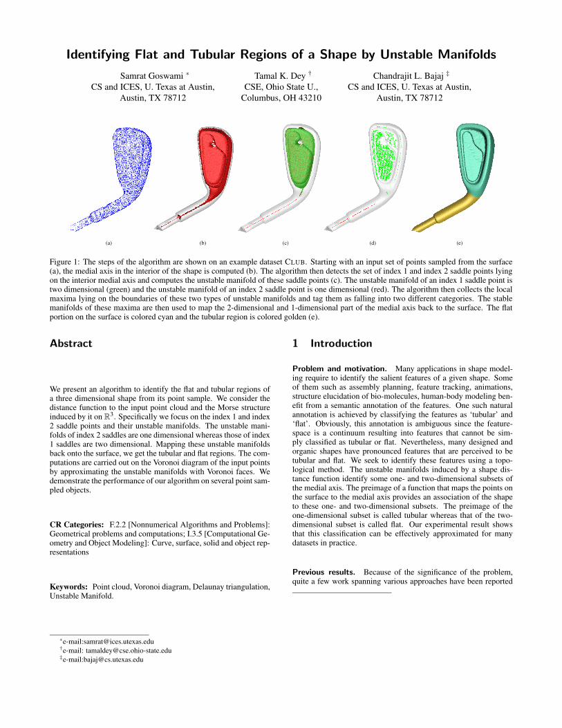
Identifying Flat and Tubular Regions of a Shape by Unstable Manifolds Samrat Goswami * CS and ICES, U. Texas at Austin, Austin, TX 78712 Tamal K. Dey † CSE, Ohio State U., Columbus, OH 43210 Chandrajit L. Bajaj ‡ CS and ICES, U. Texas at Austin, Austin, TX 78712 (a) (b) (c) (d) (e) Figure 1: The steps of the algorithm are shown on an example dataset CLUB. Starting with an input set of points sampled from the surface (a), the medial axis in the interior of the shape is computed (b). The algorithm then detects the set of index 1 and index 2 saddle points lying on the interior medial axis and computes the unstable manifold of these saddle points (c). The unstable manifold of an index 1 saddle point is two dimensional (green) and the unstable manifold of an index 2 saddle point is one dimensional (red). The algorithm then collects the local maxima lying on the boundaries of these two types of unstable manifolds and tag them as falling into two different categories. The stable manifolds of these maxima are then used to map the 2-dimensional and 1-dimensional part of the medial axis back to the surface. The flat portion on the surface is colored cyan and the tubular region is colored golden (e). Abstract We present an algorithm to identify the flat and tubular regions of a three dimensional shape from its point sample. We consider the distance function to the input point cloud and the Morse structure induced by it on R 3 . Specifically we focus on the index 1 and index 2 saddle points and their unstable manifolds. The unstable mani- folds of index 2 saddles are one dimensional whereas those of index 1 saddles are two dimensional. Mapping these unstable manifolds back onto the surface, we get the tubular and flat regions. The com- putations are carried out on the Voronoi diagram of the input points by approximating the unstable manifolds with Voronoi faces. We demonstrate the performance of our algorithm on several point sam- pled objects. CR Categories: F.2.2 [Nonnumerical Algorithms and Problems]: Geometrical problems and computations; I.3.5 [Computational Ge- ometry and Object Modeling]: Curve, surface, solid and object rep- resentations Keywords: Point cloud, Voronoi diagram, Delaunay triangulation, Unstable Manifold. * e-mail:[email protected] † e-mail: [email protected] ‡ e-mail:[email protected] 1 Introduction Problem and motivation. Many applications in shape model- ing require to identify the salient features of a given shape. Some of them such as assembly planning, feature tracking, animations, structure elucidation of bio-molecules, human-body modeling ben- efit from a semantic annotation of the features. One such natural annotation is achieved by classifying the features as ‘tubular’ and ‘flat’. Obviously, this annotation is ambiguous since the feature- space is a continuum resulting into features that cannot be sim- ply classified as tubular or flat. Nevertheless, many designed and organic shapes have pronounced features that are perceived to be tubular and flat. We seek to identify these features using a topo- logical method. The unstable manifolds induced by a shape dis- tance function identify some one- and two-dimensional subsets of the medial axis. The preimage of a function that maps the points on the surface to the medial axis provides an association of the shape to these one- and two-dimensional subsets. The preimage of the one-dimensional subset is called tubular whereas that of the two- dimensional subset is called flat. Our experimental result shows that this classification can be effectively approximated for many datasets in practice. Previous results. Because of the significance of the problem, quite a few work spanning various approaches have been reported
Transcript of Identifying Flat and Tubular Regions of a Shape by...
Identifying Flat and Tubular Regions of a Shape by Unstable Manifolds
Samrat Goswami ∗
CS and ICES, U. Texas at Austin,Austin, TX 78712
Tamal K. Dey †
CSE, Ohio State U.,Columbus, OH 43210
Chandrajit L. Bajaj ‡
CS and ICES, U. Texas at Austin,Austin, TX 78712
(a) (b) (c) (d) (e)
Figure 1: The steps of the algorithm are shown on an example dataset CLUB. Starting with an input set of points sampled from the surface(a), the medial axis in the interior of the shape is computed (b). The algorithm then detects the set of index 1 and index 2 saddle points lyingon the interior medial axis and computes the unstable manifold of these saddle points (c). The unstable manifold of an index 1 saddle point istwo dimensional (green) and the unstable manifold of an index 2 saddle point is one dimensional (red). The algorithm then collects the localmaxima lying on the boundaries of these two types of unstable manifolds and tag them as falling into two different categories. The stablemanifolds of these maxima are then used to map the 2-dimensional and 1-dimensional part of the medial axis back to the surface. The flatportion on the surface is colored cyan and the tubular region is colored golden (e).
Abstract
We present an algorithm to identify the flat and tubular regions ofa three dimensional shape from its point sample. We consider thedistance function to the input point cloud and the Morse structureinduced by it on R
3. Specifically we focus on the index 1 and index2 saddle points and their unstable manifolds. The unstable mani-folds of index 2 saddles are one dimensional whereas those of index1 saddles are two dimensional. Mapping these unstable manifoldsback onto the surface, we get the tubular and flat regions. The com-putations are carried out on the Voronoi diagram of the input pointsby approximating the unstable manifolds with Voronoi faces. Wedemonstrate the performance of our algorithm on several point sam-pled objects.
CR Categories: F.2.2 [Nonnumerical Algorithms and Problems]:Geometrical problems and computations; I.3.5 [Computational Ge-ometry and Object Modeling]: Curve, surface, solid and object rep-resentations
Keywords: Point cloud, Voronoi diagram, Delaunay triangulation,Unstable Manifold.
∗e-mail:[email protected]†e-mail: [email protected]‡e-mail:[email protected]
1 Introduction
Problem and motivation. Many applications in shape model-ing require to identify the salient features of a given shape. Someof them such as assembly planning, feature tracking, animations,structure elucidation of bio-molecules, human-body modeling ben-efit from a semantic annotation of the features. One such naturalannotation is achieved by classifying the features as ‘tubular’ and‘flat’. Obviously, this annotation is ambiguous since the feature-space is a continuum resulting into features that cannot be sim-ply classified as tubular or flat. Nevertheless, many designed andorganic shapes have pronounced features that are perceived to betubular and flat. We seek to identify these features using a topo-logical method. The unstable manifolds induced by a shape dis-tance function identify some one- and two-dimensional subsets ofthe medial axis. The preimage of a function that maps the points onthe surface to the medial axis provides an association of the shapeto these one- and two-dimensional subsets. The preimage of theone-dimensional subset is called tubular whereas that of the two-dimensional subset is called flat. Our experimental result showsthat this classification can be effectively approximated for manydatasets in practice.
Previous results. Because of the significance of the problem,quite a few work spanning various approaches have been reported

in the literature. To mention a few, we refer to the curvature basedmethods of [Varady et al. 1997] and [Mortara et al. 2004a; Mortaraet al. 2004b], the fuzzy clustering method of [Katz and Tal 2003],the method based on PCA of surface normals by [Pottmann et al.2004], the hybrid variational surface approximation by [Wu andKobbelt 2005] and the Reeb graph approach of [Shinagawa et al.1996] and [Verroust and Lazarus 2000]. Remarkably the distancefunction over R
3 which is defined by the distance to the bound-ary of the shape has not been fully used for feature annotation. Inthe context of surface reconstruction, topological structures inducedby distance functions have been analyzed by Edelsbrunner [Edels-brunner 2002], Chaine [Chaine 2003] and Giesen and John [Giesenand John 2003]. Chazal and Lieutier [Chazal and Lieutier 2004]and Siddiqi et al. [Siddiqi et al. 1998] have used it for medial axisapproximations. Dey, Giesen and Goswami used the topologicalstructures induced by the distance function to segment a shape [Deyet al. 2003]. However, this work stops short of using the topolog-ical structures for feature annotations. In this paper we completethis step.
Results. Given a compact surface Σ smoothly embedded in R3,
a distance function hΣ can be assigned over R3 that assigns to each
point its distance to Σ.
hΣ : R3 → R, x 7→ inf
p∈Σ‖x− p‖
In applications, Σ is often known via a finite set of sample points Pof Σ. Therefore it is quite natural to approximate the function hΣ bythe function
hP : R3 → R, x 7→ min
p∈P‖x− p‖
which assigns to each point in R3 the distance to the nearest sample
point in P.
In this paper, we start with a finite sample P of Σ and identify theindex 1 and index 2 saddle points of hP from the Voronoi diagramVorP and its dual Delaunay triangulation DelP of P. We then se-lect only the saddle points of both indices which lie on the interiormedial axis of Σ and compute their unstable manifolds. The un-stable manifold of index 1 saddle points (U1) are two dimensionalwhereas those of index 2 (U2) are one dimensional. Exact computa-tions of U1 is prone to numerical error. So, we present an algorithmto compute them approximately. We then map the points belongingto U1 and U2 back to Σ. The image of U1 under the mapping givesthe flat regions of Σ and that of U2 gives its tubular regions.
Thus, the main contributions of this paper are:
• Algorithms to compute the unstable manifolds of the index 2saddles points of hP exactly and those of the index 1 saddlepoints approximately,
• Identification of the tubular and flat features of Σ from its pointsample P via the unstable manifolds of the saddle points,
• Experimental results exhibiting the performance of our algo-rithm on several point sampled objects.
The paper is organized as follows. In Section 2 we state some def-initions and explain the terms such as Voronoi-Delaunay diagram,induced flow, stable/unstable manifolds etc. In Section 3 we de-scribe the relation between the Voronoi-Delaunay diagram of thepoint set P and the induced flow. In Section 4 we describe thestructure of the unstable manifolds of index 1 and index 2 saddlepoints and present an algorithm to compute them. In Section 5 wegive an algorithm to map the unstable manifolds back to the surfaceto identify its flat and tubular features. In Section 6 we demonstrate
the results of our algorithm on several models ranging from CADobjects to protein molecules. We conclude in Section 7.
2 Preliminaries
2.1 Voronoi-Delaunay Diagram of P
In this paper we always assume the distance metric to be Euclideanunless otherwise stated. For a finite set of points P in R
3, theVoronoi cell of p ∈ P is
Vp = {x ∈ R3 : ∀q ∈ P−{p}, ‖x− p‖ ≤ ‖x−q‖)}.
If the points are in general position, two Voronoi cells with non-empty intersection meet along a planar, convex Voronoi facet, threeVoronoi cells with non-empty intersection meet along a commonVoronoi edge and four Voronoi cells with non-empty intersectionmeet at a Voronoi vertex. A cell decomposition consisting of theVoronoi objects, that is, Voronoi cells, facets, edges and vertices isthe Voronoi diagram VorP of the point set P.
The dual of VorP is the Delaunay diagram DelP of P which is asimplicial complex when the points are in general position. Thetetrahedra are dual to the Voronoi vertices, the triangles are dual tothe Voronoi edges, the edges are dual to the Voronoi facets and thevertices (sample points from P) are dual to the Voronoi cells. Wealso refer to the Delaunay simplices as Delaunay objects.
2.2 Induced Flow
The distance function hP induces a flow at every point x ∈ R3. This
flow has been characterized earlier [Giesen and John 2003]. Seealso [Edelsbrunner 2002]. For completeness we briefly mention ithere.
Critical Points. The critical points of hP are those points wherehP has no non-zero gradient along any direction. These are thepoints in R
3 which lie within the convex hull of its closest pointsfrom P. It turns out that the critical points of hP are the intersectionpoints of the Voronoi objects with their dual Delaunay objects.
• Maxima are the Voronoi vertices contained in their dual tetra-hedra,
• Index 2 saddles lie at the intersection of Voronoi edges withtheir dual Delaunay triangles,
• Index 1 saddles lie at the intersection of Voronoi facets withtheir dual Delaunay edges, and
• Minima are the sample points themselves as they are alwayscontained in their Voronoi cells.
In this discrete setting, the index of a critical point is the dimen-sion of the lowest dimensional Delaunay simplex that contains thecritical point.
Flow. For every point x ∈ R3, let V (x) be the lowest dimensional
Voronoi object that contains x and D(x) be its dual. Now driver ofx, denoted as d(x), is defined as
d(x) = argminy∈D(x)‖x− y‖
The direction of steepest ascent can be uniquely determined by aunit vector in the direction of x−d(x). The critical points coincidewith their drivers. Now one can assign a vector v at every x with azero vector assigned at the critical points. The resulting vector fieldis not necessarily continuous. Nevertheless, it induces a flow in R
3.This flow tells how a point x moves in R
3 along the steepest ascentof hP and the corresponding path is known as the orbit of x. We canalso define an inverted orbit of x where x moves in the direction ofsteepest descent.
Stable and Unstable Manifolds. For a critical point c its sta-ble manifold is the set of points whose orbits end at c. The unstablemanifold of a critical point c is the set of points whose inverted or-bits end at c. The structure and computation of stable manifoldsof the critical points of hP were described in [Giesen and John2003]. They can be computed from the Delaunay triangulationsof the given point sets though they may not be subcomplexes ofthe Delaunay triangulations. For computational advantages theyare also approximated by Delaunay subcomplexes as in [Dey et al.2003].
We are interested in computing unstable manifolds and their ap-proximations. As the Delaunay and Voronoi diagrams, the struc-tures of stable and unstable manifolds have a duality. Interestingly,one can compute the unstable manifolds and their approximationsfrom the Voronoi diagrams. Here we state some of the facts aboutthe unstable manifolds of the critical points.
1. MAXIMA. The unstable manifold is the local maximum itself.
2. INDEX 2 SADDLES. The unstable manifold of an index 2 sad-dle point is a polyline starting at the saddle point and endingat a maximum.
3. INDEX 1 SADDLES. The unstable manifold of an index 1 sad-dle point is a two dimensional surface patch which is boundedby the unstable manifold of index 2 saddle points.
4. MINIMA. The unstable manifold of a local minimum is athree dimensional polytope bounded by the unstable manifoldof critical points with higher indices.
In Section 4 the computation of the unstable manifold of index 1and index 2 saddle points is described.
3 Flow on Voronoi Objects
Before we state the connection between the flow induced by hPand the Vor-Del diagram of P, we would like to state some factsabout the relative position of Voronoi and Delaunay objects. Theserelative positions can describe the nature of flows in the Voronoiobjects. These facts were clearly explained in [Edelsbrunner 2002]for a more general setting of power distance.
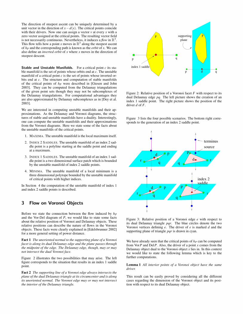
Fact 1 The unoriented normal to the supporting plane of a Voronoifacet is along its dual Delaunay edge and the plane passes throughthe midpoint of the edge. The Delaunay edge, though, may or maynot intersect the dual Voronoi face.
Figure 2 illustrates the two possibilities that may arise. The leftfigure corresponds to the situation that results in an index 1 saddlepoint.
Fact 2 The supporting line of a Voronoi edge always intersects theplane of the dual Delaunay triangle at its circumcenter and is alongits unoriented normal. The Voronoi edge may or may not intersectthe interior of the Delaunay triangle.
p qd
p q
index 1 saddle
Fsupportingplane
F
Figure 2: Relative position of a Voronoi facet F with respect to itsdual Delaunay edge pq. The left picture shows the creation of anindex 1 saddle point. The right picture shows the position of thedriver d of F .
Figure 3 lists the four possible scenarios. The bottom right corre-sponds to the generation of an index 2 saddle point.
p
qrd
p
qrd
p
qr
source
d
terminus
p
qr
index 2saddle
Figure 3: Relative position of a Voronoi edge e with respect toits dual Delaunay triangle pqr. The blue circles denote the twoVoronoi vertices defining e. The driver of e is marked d and thesupporting plane of triangle pqr is drawn in cyan.
We have already seen that the critical points of hP can be computedfrom VorP and DelP. Also, the driver of a point x comes from theDelaunay object dual to the Voronoi object x lies in. In this contextwe would like to state the following lemma which is key to thefurther computations.
Lemma 1 All interior points of a Voronoi object have the samedriver.
This result can be easily proved by considering all the differentcases regarding the dimension of the Voronoi object and its posi-tion with respect to its dual Delaunay object.
By Lemma 1 and Facts 1 and 2 we can list the possible position ofthe drivers of the points lying in the interior of a certain dimensionalVoronoi object.
Position of Drivers
Voronoi Cell
For a Voronoi cell Vp, the dual Delaunay object is a singleton setcontaining the sample point p and therefore all points x in the inte-rior of Vp has p as their driver.
Voronoi Facet
Consider a Voronoi facet in the intersection of Vp and Vq. The dualDelaunay edge is pq and the midpoint of pq is the driver of all xlying in the interior of the Voronoi facet (Figure 2(right) ).
Voronoi Edge
Next, consider a Voronoi edge in the intersection of Vp,Vq,Vr. AsFact 2 and Figure 3 indicate, the infinite line segment containingthe Voronoi edge may or may not intersect the convex hull of p,q,rleading to two different possibilities
Case 1.1 In case of intersection, the circumcenter of pqr is thedriver. Such Voronoi edges will be termed non-transversaledges as the flow is along the edge itself. The Voronoi edgehas two Voronoi vertices as its endpoints. If both of them arein the same half-space defined by pqr, the closer Voronoi ver-tex is called source and the further one is called terminus ofthe Voronoi edge because the flow is directed from the closerto the further vertex. Figure 3 (top right) illustrates this case.
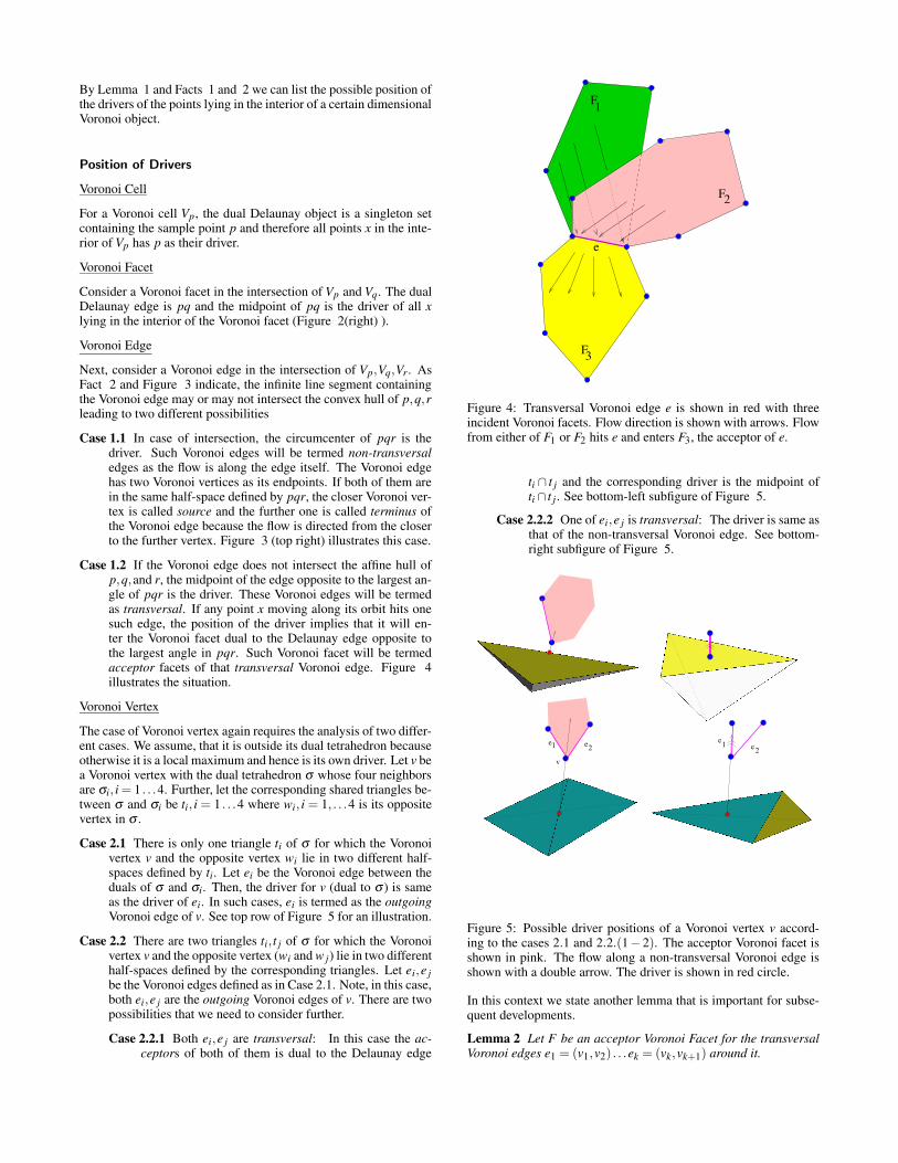
Case 1.2 If the Voronoi edge does not intersect the affine hull ofp,q,and r, the midpoint of the edge opposite to the largest an-gle of pqr is the driver. These Voronoi edges will be termedas transversal. If any point x moving along its orbit hits onesuch edge, the position of the driver implies that it will en-ter the Voronoi facet dual to the Delaunay edge opposite tothe largest angle in pqr. Such Voronoi facet will be termedacceptor facets of that transversal Voronoi edge. Figure 4illustrates the situation.
Voronoi Vertex
The case of Voronoi vertex again requires the analysis of two differ-ent cases. We assume, that it is outside its dual tetrahedron becauseotherwise it is a local maximum and hence is its own driver. Let v bea Voronoi vertex with the dual tetrahedron σ whose four neighborsare σi, i = 1 . . .4. Further, let the corresponding shared triangles be-tween σ and σi be ti, i = 1 . . .4 where wi, i = 1, . . .4 is its oppositevertex in σ .
Case 2.1 There is only one triangle ti of σ for which the Voronoivertex v and the opposite vertex wi lie in two different half-spaces defined by ti. Let ei be the Voronoi edge between theduals of σ and σi. Then, the driver for v (dual to σ ) is sameas the driver of ei. In such cases, ei is termed as the outgoingVoronoi edge of v. See top row of Figure 5 for an illustration.
Case 2.2 There are two triangles ti, t j of σ for which the Voronoivertex v and the opposite vertex (wi and w j) lie in two differenthalf-spaces defined by the corresponding triangles. Let ei,e jbe the Voronoi edges defined as in Case 2.1. Note, in this case,both ei,e j are the outgoing Voronoi edges of v. There are twopossibilities that we need to consider further.
Case 2.2.1 Both ei,e j are transversal: In this case the ac-ceptors of both of them is dual to the Delaunay edge
e
F
F
F
1
3
2
Figure 4: Transversal Voronoi edge e is shown in red with threeincident Voronoi facets. Flow direction is shown with arrows. Flowfrom either of F1 or F2 hits e and enters F3, the acceptor of e.
ti ∩ t j and the corresponding driver is the midpoint ofti ∩ t j . See bottom-left subfigure of Figure 5.
Case 2.2.2 One of ei,e j is transversal: The driver is same asthat of the non-transversal Voronoi edge. See bottom-right subfigure of Figure 5.
v
e e1 2 e1e2
Figure 5: Possible driver positions of a Voronoi vertex v accord-ing to the cases 2.1 and 2.2.(1− 2). The acceptor Voronoi facet isshown in pink. The flow along a non-transversal Voronoi edge isshown with a double arrow. The driver is shown in red circle.
In this context we state another lemma that is important for subse-quent developments.
Lemma 2 Let F be an acceptor Voronoi Facet for the transversalVoronoi edges e1 = (v1,v2) . . .ek = (vk,vk+1) around it.
1. The Voronoi edges e1 . . .ek form a continuous chain aroundF.
2. The Voronoi vertices v2 . . .vk fall in the category 2.2.1. TheVoronoi vertices v1 and vk+1 fall in the category 2.2.2.
3. F, e1 . . .ek, v2 . . .vk have same driver which is the midpoint ofthe Delaunay edge dual to F.
We omit the proofs of all of the above claims.
4 Computing Unstable Manifolds
4.1 Unstable Manifold of Index-2 Saddle Points
In this section we describe the structure and computation of theunstable manifolds of index 2 saddle points.
The unstable manifold of an index 2 saddle point is one dimen-sional. In our discrete setting it is a polyline with one endpoint at thesaddle point and the other endpoint at a local maximum. The poly-line consists of segments that are either subsets of non-transversalVoronoi edges or lie in the Voronoi facets. Due to the later case, thepolyline may not be a subcomplex of VorP.
Let us consider an index 2 saddle point, c, at the intersection ofa Delaunay triangle t with a Voronoi edge e. Let the two tetrahe-dra sharing f be σ1,σ2. The edge e has the endpoints at the dualVoronoi vertices of σ1 and σ2, denoted as v1,v2 respectively. Theunstable manifold U(c) of c, has two intervals - one from c to v1and the other from c to v2. We look at the structure of one of them,say the one from c to v1, and the other one is similar.
At any point on the subsegment cv1, the flow is toward v1 from c.Once the flow reaches v1, the subsequent flow depends on the driverof v1. Instead of just looking at v1, we consider a generic step,where the flow reaches at a Voronoi vertex v and we enumerate thepossible situations that might occur depending on the position ofdriver of v. If v is a local maximum, the flow stops there, as thedriver of v is v itself. Otherwise there are two cases to consider.
• v falls into Case 2.1: Let the dual tetrahedron be σ andthe driver of v is same as that of the Voronoi edge e whichis between the dual of σ and one of its neighbors, say σ ′. Ife is non-transversal, the flow will be along the Voronoi edgee till it hits the Voronoi vertex at the other endpoint (dual toσ ′). Otherwise, the flow enters the acceptor Voronoi facet Fof e. Due to Lemma 2, the driver of F is same as the driverof e. Therefore the next piece of the unstable manifold can beuniquely determined by the driver of e, say d and the Voronoivertex v. It is the segment between v and the point where theray
−→dv intersects a Voronoi edge of F .
• v falls under Case 2.2.x: This situation is similar to the onedescribed above. In case of both of the Voronoi edges beingtransversal (Case 2.2.1), the flow enters the acceptor Voronoifacet. In the other case (Case 2.2.2), the flow follows the non-transversal Voronoi edge.
Some segments of U(c) are not along the Voronoi edges. Whereverthe flow encounters a transversal Voronoi edge, it seizes to followthe Voronoi edge and enters a Voronoi facet which is acceptor forthat Voronoi edge. This calls for the analysis of the flow whenit crosses an acceptor Voronoi facet and hits a Voronoi edge. Wehave already characterized the position of the driver for a Voronoiedge and thereby classified those edges as either transversal or non-transversal. If the current edge intersected by the ray from the driver
to v is a non-transversal edge, the flow will follow that Voronoiedge and hit a Voronoi vertex. Otherwise, it will enter the acceptorVoronoi facet of the Voronoi edge again. There is a technical dif-ficulty we need to point out. Unless the acceptor for this Voronoiedge is different from the Voronoi facet the flow came from, wemay encounter a cycle. The following lemma saves us from thisawkward situation.
Lemma 3 Let F be a Voronoi facet and let d be its driver. Let ebe a Voronoi edge for which F is acceptor and x be any point on e.Also assume the ray from d to x intersects a Voronoi edge e′. If e′ istransversal, the acceptor of e′ is different from F.
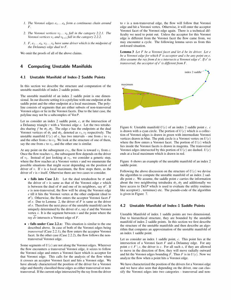
index 2 saddle
maximum
Figure 6: Unstable manifold U(c) of an index 2 saddle point c. cis drawn with a cyan circle. The portion of U(c) which is a collec-tion of Voronoi edges is drawn in green with intermediate Voronoivertices drawn in blue. The pink circle is a Voronoi vertex on U(c)where the flow enters a Voronoi facet. The portion of U(c) whichlies inside the Voronoi facets is drawn in magenta. The transversalVoronoi edges intersected by this portion of U(c) are dashed. U(c)ends at a local maximum which is drawn in red.
Figure 6 shows an example of the unstable manifold of an index 2saddle point.
Following the above discussion on the structure of U(c) we devisethe algorithm to compute the unstable manifold of an index 2 sad-dle point c. We assume, the saddle point c carries the informationabout the two neighboring tetrahedra σ1,σ2 and additionally wehave access to DelP which is used to evaluate the utility routineslike acceptor() , terminus() etc. The pseudo-code of the algorithmis given in Figure 7.
4.2 Unstable Manifold of Index-1 Saddle Points
Unstable Manifold of index 1 saddle points are two dimensional.Due to hierarchical structure, they are bounded by the unstablemanifold of index 2 saddle points. In this section we first describethe structure of the unstable manifolds and then describe an algo-rithm that computes an approximation of the unstable manifold ofan index 1 saddle point.
Let us consider an index 1 saddle point, c. This point lies at theintersection of a Voronoi facet F and a Delaunay edge. For anypoint x ∈ F \ c, the driver is c. For all such x, if they are allowedto move in the direction of flow, they will move radially outwardand hit the Voronoi edges bounding F . Thus F is in U(c). Now weanalyze the flow when a point hits a Voronoi edge.
We have characterized the position of the drivers for a Voronoi edgeand we have also seen that depending on the driver, one can clas-sify the Voronoi edges into two categories - transversal and non-
UM INDEX 2(c)1 U1 = cv1 and U2 = cv22 v = v13 end(U1) = v14 while (v is not a maximum) do5 if(v is not a Voronoi vertex)6 e = Voronoi edge containing v7 if(e is non-transversal)8 end(U1) = terminus(e)9 U1 = U1 ∪ segment(v,end(U1)
10 v = terminus(e)11 else12 F = acceptor(e)13 d = driver(F) = driver(e)14 x =
−→dv∩ e′ 6= /0, e′ is a Voronoi edge of F
15 end(U1) = x16 U1 = U1 ∪ segment(v,end(U1)17 v = x18 else19 if(v falls under Case 2.1)20 e = outgoing Voredge (v)21 repeat steps 7-17.22 else if(v falls under Case 2.2)23 F = acceptor(v)24 repeat steps 13-17.25 endwhile26 Similarly compute U2.27 return U1 ∪U2.
Figure 7: Pseudo-code for computation of unstable manifold of anindex 2 saddle point.
transversal. For a non-transversal Voronoi edge, the flow is alongthe Voronoi edge. Such Voronoi edges lie on the boundary of U(c).On the other hand, U(c) grows via the acceptor facets of transversalVoronoi edges. Depending on the position of the driver, which byLemma 2 is same for both the edge and the acceptor facet, a trun-cated cone defines the extension of U(c) into the acceptor Voronoifacet. Consider the cone defined by the two rays emanating from thedriver and passing through the endpoints of the transversal Voronoiedge. The intersection of the acceptor facet with the cone definesthe truncated cone. The truncated cone hits a continuous chain ofVoronoi edges in the acceptor facet. Some of them are completelycontained in the truncated cone and some of them are intersectedby the two rays and hence are partially contained in it. This chainof edges defines the new boundary of U(c) through some of whichU(c) can be extended further recursively. Figure 8 shows an exam-ple truncated cone in a Voronoi facet F by the driver d and the endVoronoi vertices of the transversal Voronoi edge (green).
To compute U(c) accurately, one therefore needs to compute theintersection of a ray and a line segment in three dimension. Suchcomputations are prone to numerical errors. Therefore, we rely onan approximation algorithm that computes a superset of U(c). Thealgorithm works as follows.
Starting from the Voronoi facet F containing c, we maintain a list ofVoronoi facets which are already in U(c) and a list of active Voronoiedges which are transversal edges and lie on the boundary of thecurrent approximation of U(c). Through these transversal edges wecollect their acceptor facets and grow U(c). Instead of computingthe new set of active edges by an expensive numerical calculation ofray-segment intersection, we collect all the transversal edges of thisnew acceptor Voronoi facets. This way we grow U(c) recursively
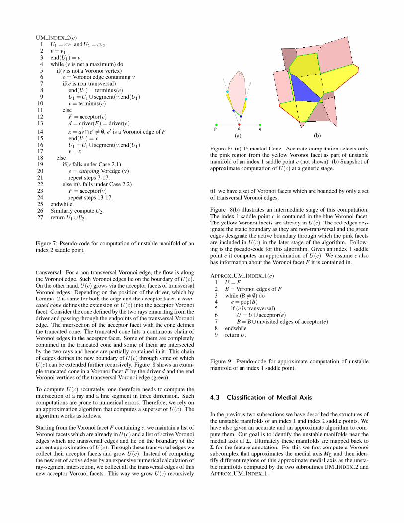
p qd
F
(a) (b)
Figure 8: (a) Truncated Cone. Accurate computation selects onlythe pink region from the yellow Voronoi facet as part of unstablemanifold of an index 1 saddle point c (not shown). (b) Snapshot ofapproximate computation of U(c) at a generic stage.
till we have a set of Voronoi facets which are bounded by only a setof transversal Voronoi edges.
Figure 8(b) illustrates an intermediate stage of this computation.The index 1 saddle point c is contained in the blue Voronoi facet.The yellow Voronoi facets are already in U(c). The red edges des-ignate the static boundary as they are non-transversal and the greenedges designate the active boundary through which the pink facetsare included in U(c) in the later stage of the algorithm. Follow-ing is the pseudo-code for this algorithm. Given an index 1 saddlepoint c it computes an approximation of U(c). We assume c alsohas information about the Voronoi facet F it is contained in.
APPROX UM INDEX 1(c)1 U = F2 B = Voronoi edges of F3 while (B 6= /0) do4 e = pop(B)5 if (e is transversal)6 U = U ∪ acceptor(e)7 B = B∪unvisited edges of acceptor(e)8 endwhile9 return U .
Figure 9: Pseudo-code for approximate computation of unstablemanifold of an index 1 saddle point.
4.3 Classification of Medial Axis
In the previous two subsections we have described the structures ofthe unstable manifolds of an index 1 and index 2 saddle points. Wehave also given an accurate and an approximate algorithm to com-pute them. Our goal is to identify the unstable manifolds near themedial axis of Σ. Ultimately these manifolds are mapped back toΣ for the feature annotation. For this we first compute a Voronoisubcomplex that approximates the medial axis MΣ and then iden-tify different regions of this approximate medial axis as the unsta-ble manifolds computed by the two subroutines UM INDEX 2 andAPPROX UM INDEX 1.
Before we describe our approach, we briefly mention a recent re-sult by Dey, Giesen, Ramos and Sadri [Dey et al. 2005] where theyproved that under sufficient sampling of Σ by P, the critical points ofhP lie either close to Σ or close to MΣ. This motivates our approach.Applying the same result, we filter out only the index 1 and index2 saddle points near MΣ instead of Σ. Further, we consider onlythe components of MΣ which lie in the interior of the solid boundedby Σ. For this purpose we use the TIGHTCOCONE algorithm byDey and Goswami [Dey and Goswami 2003]. The implementationof this algorithm is freely available in the public domain [Cocone] along with the software for medial axis approximations which iscomputed as a Voronoi subcomplex according to the algorithm byDey and Zhao [Dey and Zhao 2004]. For the purpose of reconstruc-tion, any other reconstruction algorithm also could be used [Bernar-dini et al. 1999; Bajaj et al. 1995]. Applying TIGHTCOCONE fol-lowed by medial axis approximation we get the approximate inte-rior medial axis of Σ. We perform the critical point detection onlywithin the Voronoi subcomplex that approximates this medial axis.Let us call this set of index 1 saddle points C1 and that of index 2saddle points C2. We then apply UM INDEX 2(c) for all c∈C2 andAPPROX UM INDEX 1(c) for all c ∈C1. U(c ∈C1) is two dimen-sional and U(c ∈C2) is one dimensional. Therefore, by restrictingthe unstable manifold computation only within MΣ we obtain twosubsets of MΣ. In the next section, we describe how this classifica-tion can be mapped back to Σ for automatic identification of its flatand tubular regions.
Figure 10: Removal of small patches in the tubular region via star-ring. Magenta circles indicate the centroids of these patches, greencircles are the boundary vertices which connect a patch with a lin-ear portion (red line) and cyan circle indicates where two differentpatches join at a common vertex. Blue lines are the replacementsof these small patches obtained by the starring process.
Because of sampling artifacts, sometimes the interior medial axis inthe tubular regions have a few index 1 saddle points. The unstablemanifold of these saddle points need to be detected and approxi-mated by lines. We partition the set C1 based on the connectivityof their unstable manifolds via a common edge and every partitioncreates a patch which is the union of the unstable manifolds of allthe index 1 saddle points falling into that partition. We further as-sign an importance value based on the area of the patch and sort thepatches according to their importance. One could also employ otherattributes like diameter, width etc. to evaluate the importance. Thesmall clusters are then detected either by a user-specified thresholdvalue or by simply selecting the k-smallest clusters where k is also auser-supplied parameter. These insignificant planar regions are thenapproximated by a set of straight lines emanating from the centroidof the patch to the boundary points which are connected to either apolyline (green circles in Figure 10) or another patch (cyan circlein Figure 10). We call this process starring.
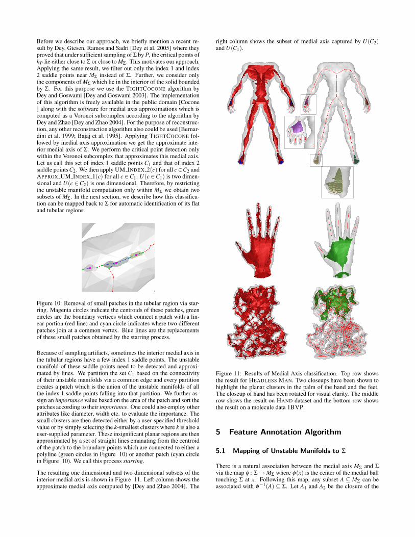
The resulting one dimensional and two dimensional subsets of theinterior medial axis is shown in Figure 11. Left column shows theapproximate medial axis computed by [Dey and Zhao 2004]. The
right column shows the subset of medial axis captured by U(C2)and U(C1).
Figure 11: Results of Medial Axis classification. Top row showsthe result for HEADLESS MAN. Two closeups have been shown tohighlight the planar clusters in the palm of the hand and the feet.The closeup of hand has been rotated for visual clarity. The middlerow shows the result on HAND dataset and the bottom row showsthe result on a molecule data 1BVP.
5 Feature Annotation Algorithm
5.1 Mapping of Unstable Manifolds to Σ
There is a natural association between the medial axis MΣ and Σvia the map φ : Σ → MΣ where φ(x) is the center of the medial balltouching Σ at x. Following this map, any subset A ⊆ MΣ can beassociated with φ−1(A) ⊆ Σ. Let A1 and A2 be the closure of the
unstable manifolds of index 2 and index 1 saddles in MΣ definedby the distance function hΣ. Recall that, generically, A1 is one-dimensional and A2 is two-dimensional. Ideally, we would like toidentify φ−1(A1) ⊆ Σ as tubular and φ−1(A2) ⊆ Σ as flat. As wehave an approximation of hΣ by hP, we compute these tubular andflat regions for the unstable manifolds in the approximate medialaxis which we denote also as MΣ for convenience.
We face a difficulty to compute an approximation of the preimageof φ from the approximate medial axis MΣ. We are interested incomputing an approximation of the preimage of M ′
Σ = A1 ∪A2 ⊆MΣ under the map φ .
Unfortunately, this requires an expensive computation to cover theentire M′
Σ which often spans a substantial portion of MΣ. A naiveapproach is to take only a sample of M′
Σ, namely the Voronoi ver-tices, and then associate them to P, a sample of Σ, via the Voronoi-Delaunay duality. This also proves useless because M ′
Σ does notcontain all the Voronoi vertices and therefore many points in P can-not be covered by this Voronoi-Delaunay duality.
It turns out that the distance function hP again proves to be usefulto establish a correspondence between Σ and M′
Σ. Recall that, thestable manifold of a critical point is a collection of points whoseorbits terminate at that critical point. Let X and Y be the set ofmaxima in A1 ⊆ M′
Σ and A2 ⊆ M′Σ respectively. Consider the stable
manifolds of the maxima in X and Y . The points in P that are inthe stable manifolds of X are associated with the tubular regionsand those in the stable manifolds of Y are associated with the flatregions. If a point belongs to the stable manifolds of maxima inX as well as in Y , we tag it arbitrarily. These points belong to theregions where a tubular part meets a flat part. Subsequently, everytriangle of the surface reconstructed by TIGHT COCONE is taggedas flat or tubular if at least two of its vertices are already marked asflat or tubular respectively.
Computation of stable manifold of maxima has been described in[Giesen and John 2003] and its approximation was given in [Deyet al. 2003]. We follow the approximate algorithm to compute thestable manifolds of the local maxima lying on M′
Σ.
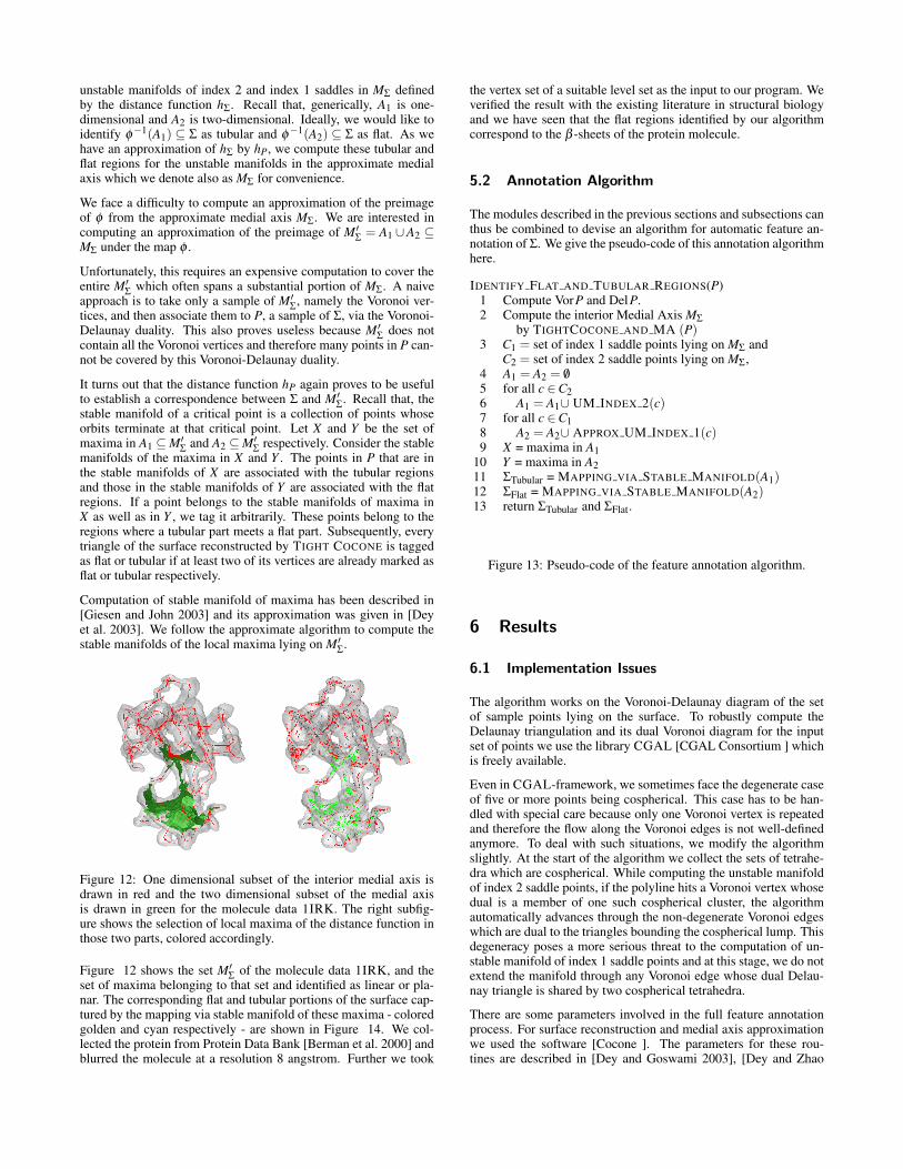
Figure 12: One dimensional subset of the interior medial axis isdrawn in red and the two dimensional subset of the medial axisis drawn in green for the molecule data 1IRK. The right subfig-ure shows the selection of local maxima of the distance function inthose two parts, colored accordingly.
Figure 12 shows the set M′Σ of the molecule data 1IRK, and the
set of maxima belonging to that set and identified as linear or pla-nar. The corresponding flat and tubular portions of the surface cap-tured by the mapping via stable manifold of these maxima - coloredgolden and cyan respectively - are shown in Figure 14. We col-lected the protein from Protein Data Bank [Berman et al. 2000] andblurred the molecule at a resolution 8 angstrom. Further we took
the vertex set of a suitable level set as the input to our program. Weverified the result with the existing literature in structural biologyand we have seen that the flat regions identified by our algorithmcorrespond to the β -sheets of the protein molecule.
5.2 Annotation Algorithm
The modules described in the previous sections and subsections canthus be combined to devise an algorithm for automatic feature an-notation of Σ. We give the pseudo-code of this annotation algorithmhere.
IDENTIFY FLAT AND TUBULAR REGIONS(P)1 Compute VorP and DelP.2 Compute the interior Medial Axis MΣ
by TIGHTCOCONE AND MA (P)3 C1 = set of index 1 saddle points lying on MΣ and
C2 = set of index 2 saddle points lying on MΣ,4 A1 = A2 = /05 for all c ∈C26 A1 = A1∪ UM INDEX 2(c)7 for all c ∈C18 A2 = A2∪ APPROX UM INDEX 1(c)9 X = maxima in A1
10 Y = maxima in A211 ΣTubular = MAPPING VIA STABLE MANIFOLD(A1)12 ΣFlat = MAPPING VIA STABLE MANIFOLD(A2)13 return ΣTubular and ΣFlat.
Figure 13: Pseudo-code of the feature annotation algorithm.
6 Results
6.1 Implementation Issues
The algorithm works on the Voronoi-Delaunay diagram of the setof sample points lying on the surface. To robustly compute theDelaunay triangulation and its dual Voronoi diagram for the inputset of points we use the library CGAL [CGAL Consortium ] whichis freely available.
Even in CGAL-framework, we sometimes face the degenerate caseof five or more points being cospherical. This case has to be han-dled with special care because only one Voronoi vertex is repeatedand therefore the flow along the Voronoi edges is not well-definedanymore. To deal with such situations, we modify the algorithmslightly. At the start of the algorithm we collect the sets of tetrahe-dra which are cospherical. While computing the unstable manifoldof index 2 saddle points, if the polyline hits a Voronoi vertex whosedual is a member of one such cospherical cluster, the algorithmautomatically advances through the non-degenerate Voronoi edgeswhich are dual to the triangles bounding the cospherical lump. Thisdegeneracy poses a more serious threat to the computation of un-stable manifold of index 1 saddle points and at this stage, we do notextend the manifold through any Voronoi edge whose dual Delau-nay triangle is shared by two cospherical tetrahedra.
There are some parameters involved in the full feature annotationprocess. For surface reconstruction and medial axis approximationwe used the software [Cocone ]. The parameters for these rou-tines are described in [Dey and Goswami 2003], [Dey and Zhao
2004]. For noisy inputs we replace TIGHT COCONE by ROBUSTCOCOCNE and the parameters for that step are again described in[Dey and Goswami 2004]. The rest of the algorithm requires onlyone parameter k which is the number of flat regions to be output.
6.2 Performance
(a)(b)
(c) (d)
(e) (f)
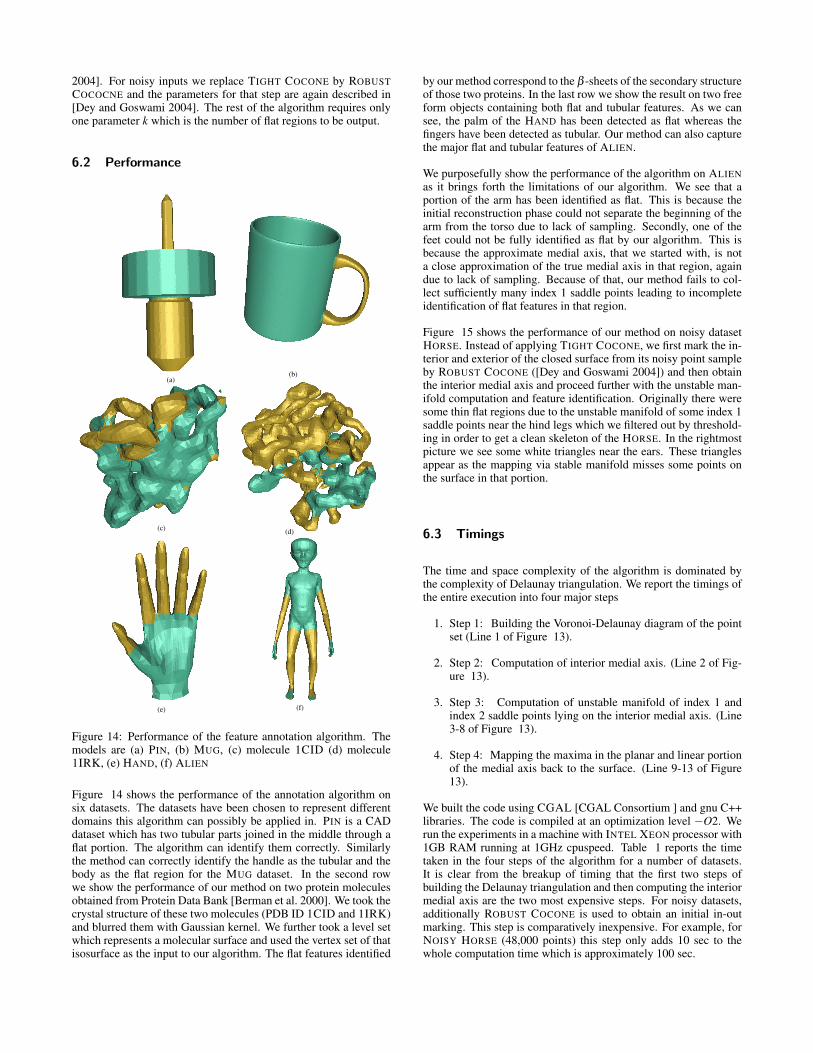
Figure 14: Performance of the feature annotation algorithm. Themodels are (a) PIN, (b) MUG, (c) molecule 1CID (d) molecule1IRK, (e) HAND, (f) ALIEN
Figure 14 shows the performance of the annotation algorithm onsix datasets. The datasets have been chosen to represent differentdomains this algorithm can possibly be applied in. PIN is a CADdataset which has two tubular parts joined in the middle through aflat portion. The algorithm can identify them correctly. Similarlythe method can correctly identify the handle as the tubular and thebody as the flat region for the MUG dataset. In the second rowwe show the performance of our method on two protein moleculesobtained from Protein Data Bank [Berman et al. 2000]. We took thecrystal structure of these two molecules (PDB ID 1CID and 1IRK)and blurred them with Gaussian kernel. We further took a level setwhich represents a molecular surface and used the vertex set of thatisosurface as the input to our algorithm. The flat features identified
by our method correspond to the β -sheets of the secondary structureof those two proteins. In the last row we show the result on two freeform objects containing both flat and tubular features. As we cansee, the palm of the HAND has been detected as flat whereas thefingers have been detected as tubular. Our method can also capturethe major flat and tubular features of ALIEN.
We purposefully show the performance of the algorithm on ALIENas it brings forth the limitations of our algorithm. We see that aportion of the arm has been identified as flat. This is because theinitial reconstruction phase could not separate the beginning of thearm from the torso due to lack of sampling. Secondly, one of thefeet could not be fully identified as flat by our algorithm. This isbecause the approximate medial axis, that we started with, is nota close approximation of the true medial axis in that region, againdue to lack of sampling. Because of that, our method fails to col-lect sufficiently many index 1 saddle points leading to incompleteidentification of flat features in that region.
Figure 15 shows the performance of our method on noisy datasetHORSE. Instead of applying TIGHT COCONE, we first mark the in-terior and exterior of the closed surface from its noisy point sampleby ROBUST COCONE ([Dey and Goswami 2004]) and then obtainthe interior medial axis and proceed further with the unstable man-ifold computation and feature identification. Originally there weresome thin flat regions due to the unstable manifold of some index 1saddle points near the hind legs which we filtered out by threshold-ing in order to get a clean skeleton of the HORSE. In the rightmostpicture we see some white triangles near the ears. These trianglesappear as the mapping via stable manifold misses some points onthe surface in that portion.
6.3 Timings
The time and space complexity of the algorithm is dominated bythe complexity of Delaunay triangulation. We report the timings ofthe entire execution into four major steps
1. Step 1: Building the Voronoi-Delaunay diagram of the pointset (Line 1 of Figure 13).
2. Step 2: Computation of interior medial axis. (Line 2 of Fig-ure 13).
3. Step 3: Computation of unstable manifold of index 1 andindex 2 saddle points lying on the interior medial axis. (Line3-8 of Figure 13).
4. Step 4: Mapping the maxima in the planar and linear portionof the medial axis back to the surface. (Line 9-13 of Figure13).
We built the code using CGAL [CGAL Consortium ] and gnu C++libraries. The code is compiled at an optimization level −O2. Werun the experiments in a machine with INTEL XEON processor with1GB RAM running at 1GHz cpuspeed. Table 1 reports the timetaken in the four steps of the algorithm for a number of datasets.It is clear from the breakup of timing that the first two steps ofbuilding the Delaunay triangulation and then computing the interiormedial axis are the two most expensive steps. For noisy datasets,additionally ROBUST COCONE is used to obtain an initial in-outmarking. This step is comparatively inexpensive. For example, forNOISY HORSE (48,000 points) this step only adds 10 sec to thewhole computation time which is approximately 100 sec.
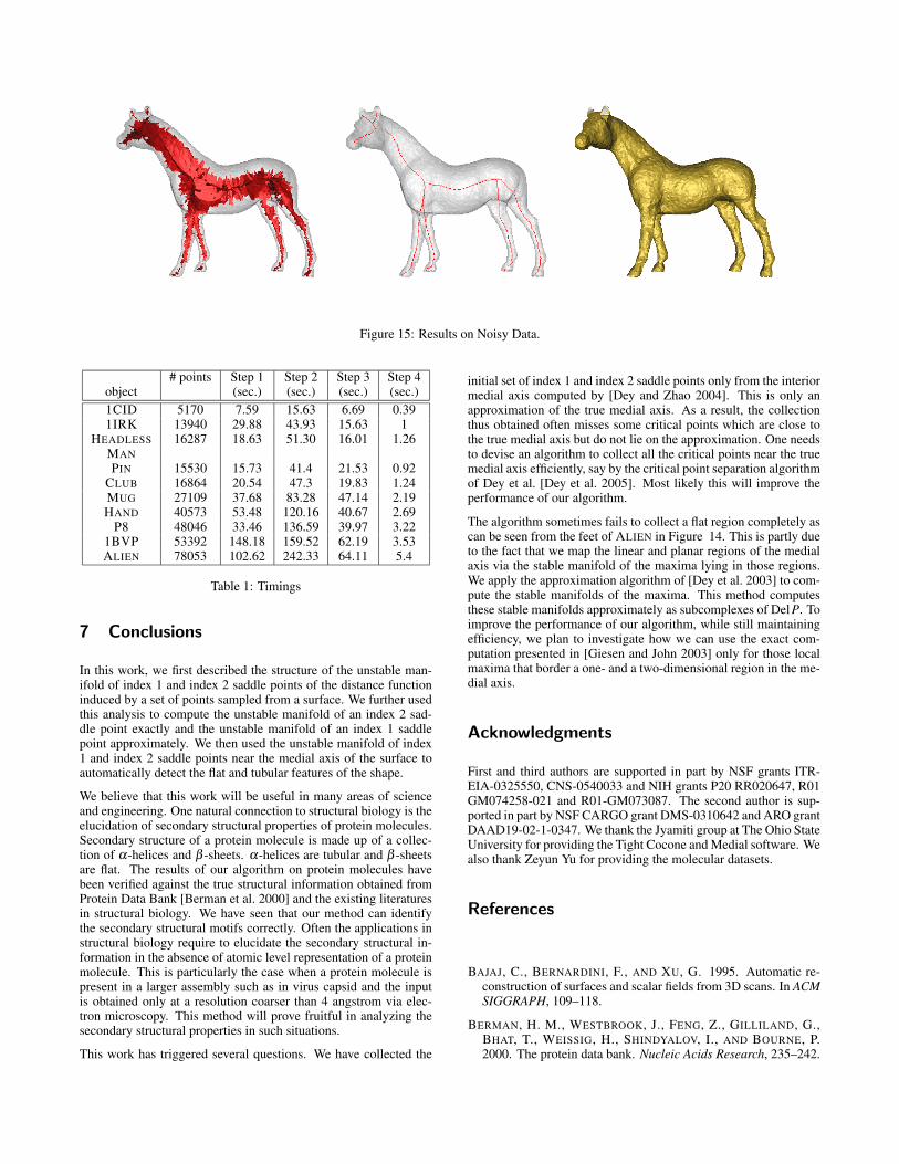
Figure 15: Results on Noisy Data.
# points Step 1 Step 2 Step 3 Step 4object (sec.) (sec.) (sec.) (sec.)1CID 5170 7.59 15.63 6.69 0.391IRK 13940 29.88 43.93 15.63 1
HEADLESS 16287 18.63 51.30 16.01 1.26MANPIN 15530 15.73 41.4 21.53 0.92
CLUB 16864 20.54 47.3 19.83 1.24MUG 27109 37.68 83.28 47.14 2.19HAND 40573 53.48 120.16 40.67 2.69
P8 48046 33.46 136.59 39.97 3.221BVP 53392 148.18 159.52 62.19 3.53ALIEN 78053 102.62 242.33 64.11 5.4
Table 1: Timings
7 Conclusions
In this work, we first described the structure of the unstable man-ifold of index 1 and index 2 saddle points of the distance functioninduced by a set of points sampled from a surface. We further usedthis analysis to compute the unstable manifold of an index 2 sad-dle point exactly and the unstable manifold of an index 1 saddlepoint approximately. We then used the unstable manifold of index1 and index 2 saddle points near the medial axis of the surface toautomatically detect the flat and tubular features of the shape.
We believe that this work will be useful in many areas of scienceand engineering. One natural connection to structural biology is theelucidation of secondary structural properties of protein molecules.Secondary structure of a protein molecule is made up of a collec-tion of α-helices and β -sheets. α-helices are tubular and β -sheetsare flat. The results of our algorithm on protein molecules havebeen verified against the true structural information obtained fromProtein Data Bank [Berman et al. 2000] and the existing literaturesin structural biology. We have seen that our method can identifythe secondary structural motifs correctly. Often the applications instructural biology require to elucidate the secondary structural in-formation in the absence of atomic level representation of a proteinmolecule. This is particularly the case when a protein molecule ispresent in a larger assembly such as in virus capsid and the inputis obtained only at a resolution coarser than 4 angstrom via elec-tron microscopy. This method will prove fruitful in analyzing thesecondary structural properties in such situations.
This work has triggered several questions. We have collected the
initial set of index 1 and index 2 saddle points only from the interiormedial axis computed by [Dey and Zhao 2004]. This is only anapproximation of the true medial axis. As a result, the collectionthus obtained often misses some critical points which are close tothe true medial axis but do not lie on the approximation. One needsto devise an algorithm to collect all the critical points near the truemedial axis efficiently, say by the critical point separation algorithmof Dey et al. [Dey et al. 2005]. Most likely this will improve theperformance of our algorithm.
The algorithm sometimes fails to collect a flat region completely ascan be seen from the feet of ALIEN in Figure 14. This is partly dueto the fact that we map the linear and planar regions of the medialaxis via the stable manifold of the maxima lying in those regions.We apply the approximation algorithm of [Dey et al. 2003] to com-pute the stable manifolds of the maxima. This method computesthese stable manifolds approximately as subcomplexes of DelP. Toimprove the performance of our algorithm, while still maintainingefficiency, we plan to investigate how we can use the exact com-putation presented in [Giesen and John 2003] only for those localmaxima that border a one- and a two-dimensional region in the me-dial axis.
Acknowledgments
First and third authors are supported in part by NSF grants ITR-EIA-0325550, CNS-0540033 and NIH grants P20 RR020647, R01GM074258-021 and R01-GM073087. The second author is sup-ported in part by NSF CARGO grant DMS-0310642 and ARO grantDAAD19-02-1-0347. We thank the Jyamiti group at The Ohio StateUniversity for providing the Tight Cocone and Medial software. Wealso thank Zeyun Yu for providing the molecular datasets.
References
BAJAJ, C., BERNARDINI, F., AND XU, G. 1995. Automatic re-construction of surfaces and scalar fields from 3D scans. In ACMSIGGRAPH, 109–118.
BERMAN, H. M., WESTBROOK, J., FENG, Z., GILLILAND, G.,BHAT, T., WEISSIG, H., SHINDYALOV, I., AND BOURNE, P.2000. The protein data bank. Nucleic Acids Research, 235–242.

BERNARDINI, F., BAJAJ, C., CHEN, J., AND SCHIKORE, D.1999. Automatic reconstruction of 3d cad models from digitalscans. Int. J. on Comp. Geom. and Appl. 9, 4-5, 327–369.
CGAL CONSORTIUM. CGAL: Computational Geometry Algo-rithms Library. http://www.cgal.org.
CHAINE, R. 2003. A geometric convection approach of 3-d recon-struction. In Proc. Eurographics Sympos. on Geometry Process-ing, 218–229.
CHAZAL, F., AND LIEUTIER, A. 2004. Stability and homotopyof a subset of the medial axis. In Proc. 9th ACM Sympos. SolidModeling and Applications, 243–248.
COCONE. Tight Cocone Software for surface reconstruc-tion and medial axis approximation. http://www.cse.ohio-state.edu/∼tamaldey/cocone.html.
DEY, T. K., AND GOSWAMI, S. 2003. Tight cocone: A water-tightsurface reconstructor. In Proc. 8th ACM Sympos. Solid Modelingand Applications, 127–134.
DEY, T. K., AND GOSWAMI, S. 2004. Provable surface recon-struction from noisy samples. In Proc. 20th ACM-SIAM Sympos.Comput. Geom., 330–339.
DEY, T. K., AND ZHAO, W. 2004. Approximating the Medial axisfrom the Voronoi diagram with convergence guarantee. Algo-rithmica 38, 179–200.
DEY, T. K., GIESEN, J., AND GOSWAMI, S. 2003. Shape segmen-tation and matching with flow discretization. In Proc. WorkshopAlgorithms Data Strucutres (WADS 03), F. Dehne, J.-R. Sack,and M. Smid, Eds., LNCS 2748, 25–36.
DEY, T. K., GIESEN, J., RAMOS, E., AND SADRI, B. 2005. Crit-ical points of the distance to an epsilon-sampling of a surfaceand flow-complex-based surface reconstruction. In Proc. 21stACM-SIAM Sympos. Comput. Geom., 218–227.
EDELSBRUNNER, H. 2002. Surface reconstruction by wrappingfinite point sets in space. In Ricky Pollack and Eli GoodmanFestschrift, B. Aronov, S. Basu, J. Pach, and M. Sharir, Eds.Springer-Verlag, 379–404.
GIESEN, J., AND JOHN, M. 2003. The flow complex: a data struc-ture for geometric modeling. In Proc. 14th ACM-SIAM Sympos.Discrete Algorithms, 285–294.
KATZ, S., AND TAL, A. 2003. Hierarchical mesh decompositionusing fuzzy clustering and cuts. In Trans. on Graphics, vol. 3,954–961.
MORTARA, M., PATANE, G., SPAGNUOLO, M., FALCIDIENO, B.,AND ROSSIGNAC, J. 2004. Blowing bubbles for the multi-scaleanalysis and decomposition of triangle meshes. Algorithmica 38,227–248.
MORTARA, M., PATANE, G., SPAGNUOLO, M., FALCIDIENO, B.,AND ROSSIGNAC, J. 2004. Plumber: a multi-scale decomposi-tion of 3d shapes into tubular primitives and bodies. In Proc. 9thACM Sympos. Solid Modeling and Applications, 139–158.
POTTMANN, H., HOFER, M., ODEHNAL, B., AND WALLNER, J.2004. Line geometry for 3d shape understanding and reconstruc-tion. Computer Vision - ECCV 3021, 1, 297–309.
SHINAGAWA, Y., KUNNI, T., BELAYEV, A., AND TSUKIOKA, T.1996. Shape modeling and shape analysis based on singularities.Internat. J. Shape Modeling 2, 85–102.
SIDDIQI, K., SHOKOUFANDEH, A., DICKINSON, J., ANDZUCKER, S. 1998. Shock graphs and shape matching. Com-puter Vision, 222–229.
VARADY, T., MARTIN, R., AND COX, J. 1997. Reverse engi-neering of geometric models - an introduction. Computer AidedDesign 29, 255–268.
VERROUST, A., AND LAZARUS, F. 2000. Extracting skeletalcurves from 3d scattered data. The Visual Computer 16, 15–25.
WU, J., AND KOBBELT, L. 2005. Structure recovery via hybridvariational surface approximation. Computer Graphics Forum24, 3, 277–284.