Identifying efficient operations through linking measurements and models in commercial buildings I: Model development and Calibration

Rongxin Yin1, 2, Sila Kiliccote1, Mary Ann Piette1, 1Lawrence Berkeley National Laboratory, Berkeley, CA 94720

2University of California at Berkeley, Berkeley, CA Abstract The use of simulation to evaluate control of low energy operations, commissioning problems, and strategies for demand response events offers new insight into building operations. This paper discusses how measured end-use energy data from a campus building were used to calibrate a simulation model developed in EnergyPlus. The building geometry and internal thermal zones were modeled to match the actual heating ventilation and air conditioning (HVAC) zoning for each individual variable air-volume (VAV) zone. We described the step-by-step procedure to calibrate the simulation model and identify key input parameters. Most key building and HVAC system components, including space loads (actual occupancy number, lighting and plug loads), HVAC air-side components (VAV terminals, supply & return fans) and water-side components (chillers, pumps, and cooling towers) were evaluated. Compared to the initial model, the results show that this process greatly improves the accuracy of the calibrated EnergyPlus model in terms of the whole building energy usage and each end-use. In addition, this approach is compared to other existing methods of model calibration to evaluate the advantage and disadvantage of each approach with this case study. Finally, this paper describes the application of the calibrated model for analyses of control systems and demand response (DR) strategies to achieve the peak demand reduction. A comparison of end-use data from modeled and actual DR events is presented. Keywords: Model calibration; Automated model calibration; Demand response; DR strategies; Demand reduction; Peak demand 1 Introduction The engineering, controls and buildings research community is developing a number of building energy optimization and advanced control concepts to reduce energy use and provide demand response capabilities in buildings. To ensure that the effect of these optimal control strategies can be evaluated with high accuracy and there is a need to develop a detailed simulation model with high level of accuracy for each building mechanical system component. The objective of this project was to evaluate if the building can deliver 30% demand reduction during an automated demand response (AutoDR) event through intelligent management of central and distributed control systems. The well calibrated simulation model will be implemented into the building energy management system (BEMS) to assist the building operators to predict the effect of various control strategies. For modelers, the most advantage of building simulation physical model could enable to perform various design strategies, analysis of various energy conversation measures (ECMs), and different building system operational modes and then choose the optimal operation scheme for achieving the proposed target, such as demand reduction, energy efficiency. So it is pretty “dynamic”. However, the biggest challenge is how to build valid and credible simulation models with less effort. If the model is not a “close” approximation to the actual building, any results or conclusions derived from the model could be erroneous and may results in costly decisions being made. Thus it needs to be “calibrated”. As more and more building information becomes available, a critical problem is enabling the simple and efficient exchange of this data between the building and the energy simulation model.

2 Model development Figure 1 shows the general procedure of the simulation model development and calibration. Generally, the goal of the model calibration is to achieve a good model by eliminating the uncertainties with the model inputs. There are limited assumptions and uncertainties with the building model itself including building geometry and envelope, while there are many uncertainties with other model inputs such as weather data, internal loads, and HVAC system components’ actual performance. Therefore, the level of the model accuracy depends on how much information can be available from the building. The author has introduced the general procedure of model development and calibration in another paper (R.Yin et.al, 2010).

Figure 1: General Procedure of Model Development and Calibration

2.1 Building description The case study building is an existing office building on campus which was built in 2008. It is 141,000 square feet, with classrooms, offices, laboratories and a 149-seat auditorium. The building is composed of an office portion and a nanofabrication lab. There are several issues that require special attention in this facility. First of all, a silicon wafer fabrication laboratory with a large clean room occupies several floors of the building. The chilled water loop of the building is shared with this laboratory. The building operator requested that no services be changed in this part of the building under any circumstances. Also, the building has two 600 ton chillers; one of them is a steam powered absorption chiller and the other is an electric centrifugal chiller. In terms of two chillers’ operation, the centrifugal chiller is operating during the winter for achieving higher plant efficiency and the absorption chilled is used during the summer for utilizing redundant resource of steam on campus. At any given time, only one of the chillers is operating and even then, the chiller is grossly over-sized for the loads in the building causing the chiller to short cycle excessively. As shown in below figures, there are two main substations, MSA and MSB, which have multiple panels that are already submetered. Some of the panels are shared between the nanofabrication lab and the offices as indicated in legends with difference colors. The office portion of SDH includes panels CH2,

CD41A, ATS-E01, and ATS-ES, ATS-MDC, CD4RA and CB4A. More details about key components at each panel are as follows:

• CH2: electric chiller (CH2) provides cooling to the whole building SDH; • CD41A: HWP-1 and HWP-2 provide hot water to all the air handling units and reheat systems;

AHU-3 and AHU-4 serve the electrical rooms at 1st floor; • ATS-E01: CHP-1 and CHP-2 (chilled water pump) and CWP-3 and CWP-4 (condenser water

pump) are the primary pumps associate with absorption/electric chillers and cooling towers (CT-1 and CT-2) to transport the chilled water to the office portion’s AHUs and the nano lab’s secondary chilled water system;

• ATS-ES: chiller multistack and associated chilled water pumps (CHP-4, CHP-5) and condenser water pumps (CWP-5, CWP-6) provide cooling to the campus IT equipment; CT-1 and CT-2 (cooling tower) associate with the absorption/electric chillers to provide cooling to SDH; roof-top units (RTU-1 and RUT-2) are used to condition and circulate air to the electrical rooms in the office portion of SDH;

• CB4A: submetered lighting and receptacle loads at each floor; The nanofabrication lab of SDH includes panels MS41A, MS41B, ATS-EL, and ATS-E01 (shared with office portion).

Figure 2: SDH Submetering Diagram - MSA

Figure 3: SDH Submetering Diagram - MSB

This study focus on the office-side building system operation since the system on nanofabrication lab cannot be touched due to the security issue. The control strategy of global temperature setpoints adjustment is proposed to test the response of the HVAC system to the zonal temperature setpoints. However, there has been a challenge to quantify the demand power reduction on demand response event days. For this reason, a regression approach to classification is brought into this study for the baseline development and be used to evaluate the effect of the proposed control strategy on the peak demand power. 2.2 Model development The initial EnergyPlus model created for SDH followed the standard practices for advanced energy model creation; the physical structure was modeled including appropriate mechanical system modules and standard ASHRAE assumptions for weather, ventilation, lighting, plug loads and other attributes of the facility. Detailed modules that correspond to the actual VAV zones were also modeled. Yet even with this substantial effort, energy usage results generated by the model differed significantly from the actual performance. Figure 4 shows the 3D model of this case study building.

Figure 4: 3D Image of the EnergyPlus Simulation Model

2.2.1 Weather data Weather is one of the most important factors in predicting the building energy performance. Specifically, real weather data is necessary for calibrating the simulation model with the measured data in buildings. Traditionally, energy model practitioners use weather data from the National weather station nearest to the site. In this study, an onsite weather station is used to capture the variability of micro-climate in the area where the building is located. A full set of weather data points was collected from the local onsite station, including the dry-bulb temperature, the dew temperature, the relative humidity, the solar radiation, the wind speed/direction and the precipitation. Those weather data points were customized into the EnergyPlus weather file to be used into simulation. 2.2.2 Zoning The general concept of zoning an energy model is simplifying the model while maintaining a reasonable level of accuracy. The level of model simplification depends on the purpose of model usage, such as architecture design, code compliance, green building rating system, ECM (Energy Conservation Measures) analysis and others. For the typical usage of the model, the general criteria are listed as follows:

• Zone functionality: For zones with different usage, each has its own space load densities (people, lighting and plug loads) and corresponding operational schedules.

• Orientation: For zones in different orientation, the load profile is unique between each other due to the change of the hourly solar gains even those zones have the similar usage.

• Thermostat control: Any rooms that are combined into a single thermal zone should have the same heating and cooling setpoints and the same Thermostat schedules.

• Perimeter/interior zone: Perimeter areas should be zoned separately from interior spaces, with the depth of perimeter zoning typically 12-15 feet from the exterior wall, in order to avoid the offset between the heating load from outdoor environment and the cooling load from the interior zones.

Specifically, for the modelling of existing buildings, the key point is to utilize all available information in buildings. In this study, A Building Management System (BMS) provides each building system component’s characteristics. Taking a variable air volume (VAV) box as the example, a full set of parameters including minimum/maximum airflow rates under cooling/heating mode, the damper position and the reheat coil valve position can be derived from the BMS. Therefore, the criteria of VAV terminal component-based zoning was followed as the 1st priority among those above criteria. The advantage of this approach is to capture the actual performance of VAV terminals and make the calibration more feasible as the first step.

Figure 5: Zoning of the 4th floor in Case Study Building

2.2.3 Internal loads Most of buildings don’t have the submetering system for monitoring each building system component’s energy usage. However, the actual performance of the space load could significantly differ from the proposed operation. During the process of initial model development, the best way to simulate the space load is following the relevant code or standard. ASHRAE standard 62.1 and 90.1 is used to determine the occupant density and the lighting & plug load densities in each type of zone, respectively. The following baseline data were used:

• Lights = 10.76 W/m2 (1.0 W/ft2) • Plug Loads = 10.76 W/m2 (1.0W /ft2) (Building Area Method) • Operating Schedules: ASHRAE 90.1-1989, Section 13

Figure 6 shows the standard inputs of the operation weekday & weekend schedules of the lighting and plug loads. Those inputs would be used if there is no submetering available in the building.

Figure 6: Lighting & Plug Load Hourly Schedules (Title 24)

2.2.4 Building system loads Equipment specifications and building HVAC schedules provide all required important characteristics for each system component, including air-side components (VAVs, AHUs, return & exhaust fans, etc.) and water-side components (chillers, cooling towers, chilled/condenser water pumps, rooftop AC units, etc.). For each component, all key parameters are identified as shown in Table 1.

Table 1: Key parameters of building HVAC system components

Air-side components Parameters Water-side components Parameters

Thermostat setpoints Each system control zone’s thermostat temperature setpoint

Steam absorption chiller

Nominal capacity, entering/leaving water temperature and flow rate at evaporator and condenser, steam load at generator, associated pump power, operating temperature setpoints

VAV terminals Minimum/maximum airflow rates under cooling/heating mode

Electric centrifugal chiller

Nominal capacity, COP, entering/leaving water temperature and flow rate at evaporator and condenser, operating temperature setpoints, operating curves

Supply/return fans in AHUs

Supply airflow rate, supply fan power, pressure, part load curve

Pumps Type, water flow rate, nominal power

Exhaust fans Fan power, airflow rate, operating efficiency Cooling towers Nominal capacity,

entering/leaving water

temperature and flow rate at design condition, tower fan power, part load curve, operating temperature setpoints

Coils in AHUs

Cooling capacity, entering/leaving chilled water temperature, water flow rate

Rooftop units Nominal capacity, characteristics of supply fan and cooling coil

3 Model calibration The general purpose of the model calibration is to achieve more accurate and better simulation results that can match to the measured data within a good agreement. Several standards and guidelines provide the acceptable calibration tolerance of the cumulative variation of root mean squared error (CVRMSE) and the mean bias error (MBE) for annual, monthly and hourly data calibration, which could guide the modelers to calibrate the simulation model until it satisfies all criteria.

Error! Reference source not found. presents the acceptable tolerance for monthly and hourly data calibration according to ASHRAE Guideline 14. The initial models were calibrated to achieve the acceptable monthly tolerances based on the required MBE and CV(RSME) then again calibrated based on hourly data to achieve a higher level of accuracy.

Table 2: Acceptable Calibration Tolerances

Calibration Type Index Acceptable Value ±5%

Monthly 15%

±10% Hourly

30% In this study the purpose of the model calibration was not only to evaluate the whole building energy performance, but to provide accurate simulation results of major building system components for better capturing the effect of various demand response strategies. Generally, the model will be calibrated to the level of the whole building utility measurements. However, in some cases, a model with good calibration of the whole building energy usage doesn’t mean that this model can provide accurate results for each breakdown end-uses. Therefore, we started to calibrate the model by the level of each component end-use, such as lighting, plug, supply fans, chillers and other sub-metering end-uses. As a result, the whole building energy usage can be easily calibrated afterwards.

The Simple Measuring and Actuation Profile (sMAP) is developed for allowing instruments and other producers of physical information to directly publish their data, which is a great tool for buildings, organizing and querying large repositories of physical data from Building Management System (BMS). Therefore, there is a good opportunity here to bridge the sMAP and the EnergyPlus simulation model by exchanging the monitoring data points and the model data inputs. Another advantage of this data exchange is speeding up the process of model calibration instead of manually validate the model data inputs. At the same time, the process of model calibration can be off-line and real-time online. Most previous research work in the field of model development and calibration focus on the whole building level to evaluate the effects of energy conservation measures (ECMs), building HVAC system control strategies and so on. For a commercial building, the whole building energy usage is composed of HVAC system, lighting, plug and miscellaneous load. The well calibrated model in the whole building level may give an unreasonable breakdown of the sub-utility level. Especially for the purpose of demand response study, demand power savings come from each load category in terms of fan, chiller, pump, cooling tower, and lighting & plug loads. Therefore, it is very necessary to validate all relevant system components’ performance to achieve a high level of model accuracy. Generally, the building geometry and envelope is modelled as it is, there is limited potential of model calibration with this component once those are verified by a field walk-in survey. As mentioned above, the key point during this process is to define the internal thermal zones within the building. There is a commonly known trade-off between the zoning simplification, the simulation speed and the model accuracy. Afterwards, component-based calibration will be went through to verify space loads, HVAC system and plant loads step by step. Another similar study descries this evidence-based model calibration methodology (P. Raftery et.al, 2011) and monitoring-based HVAC commissioning method (Wang et.al, 2013).

Figure 7: Schematic of Automated EnergyPlus Model Calibration

3.1 Internal loads Usually, the space loads account for nearly 1/3 of the whole building power usage in commercial office buildings (DOE reference of commercial building survey). Through the field walk-in survey, it is easy to estimate the number of people and behaviour in the building. However, most of buildings don’t have the sub-metering system to measure the actual power usage of the lighting and plug load. It turns out to be the wrong estimation of lighting and plug loads and the following simulations of the HVAC system and plant loads. With the increasing implementation of sub-metering system in buildings, it well resolves the above problem with the estimation. In this study, an approach was proposed by combining the sub-floor level lighting metering system and field plug load audit to feed the actual lighting & plug load densities and schedules into the model. As shown in Figure 8, the actual power usage of the lighting and plug loads can be accessed via sMAP and feed into the model either offline or real-time.

Figure 8: Sub-floor metered lighting and plug power usages (a week in 2010)

3.2 Air-side components 3.2.1 VAVs Taking the advantage of VAV-based zoning approach, the physical data points from sMAP were derived and fed into the model, including each control zone’s thermostat temperature setpoint, minimum/maximum airflow rates under heating/cooling mode. All those parameters are essential to capture the zone-by-zone thermal load and corresponding VAV performance. As shown in Figure 9, it can be clearly seen that the significant difference between the simulated airflow rate and the designed airflow rate. In fact, most of VAV terminals are oversized with higher minimum airflow rates which cause the discrepancy of the supply fan airflow rate under cold or cool weather conditions. Therefore, this discrepancy between the standard and the designed ventilation rate could lead to lower fan power predictions when most of VAVs are running at the minimum mode. On the other hand, nearly 30% of difference between the measured and the standard minimum ventilation rate provides such a potential of ventilation rate adjustment to achieve the demand reduction from building HVAC systems.

Figure 9: Comparison between the simulated airflow rate and designed airflow rates

3.2.2 AHUs Curve fitting and validation With regard to the fan power calibration, the part load curve can have a major impact on the simulated fan power usage. The actual operational curve can be different from its referenced curve from manufactures or laboratories. Therefore, the key is to derive the operational curve from the measured data. Usually there are more than two parallel fans in AHU and it is not easy to simulate this kind of fan configuration with some simulation tools. If those parallel fans are identical and running at the similar operational mode, a virtual big fan can be created to instead parallel fans by fitting an accurate part load curve. Given a set of the measured data points of supply airflow rate and fan power percentage, the actual fan operational curve of part load performance was developed. Due to the limited range of fan operation, two virtual points were put into the data set to stand for the operational condition when supply fan will be running at 100% load. However, there are still large missing ranges of fan operation condition which cannot be achieved from monitoring system. In order to ensure the accuracy of the new operational curve, another new set of data points were derived from monitoring system to validate the curve.

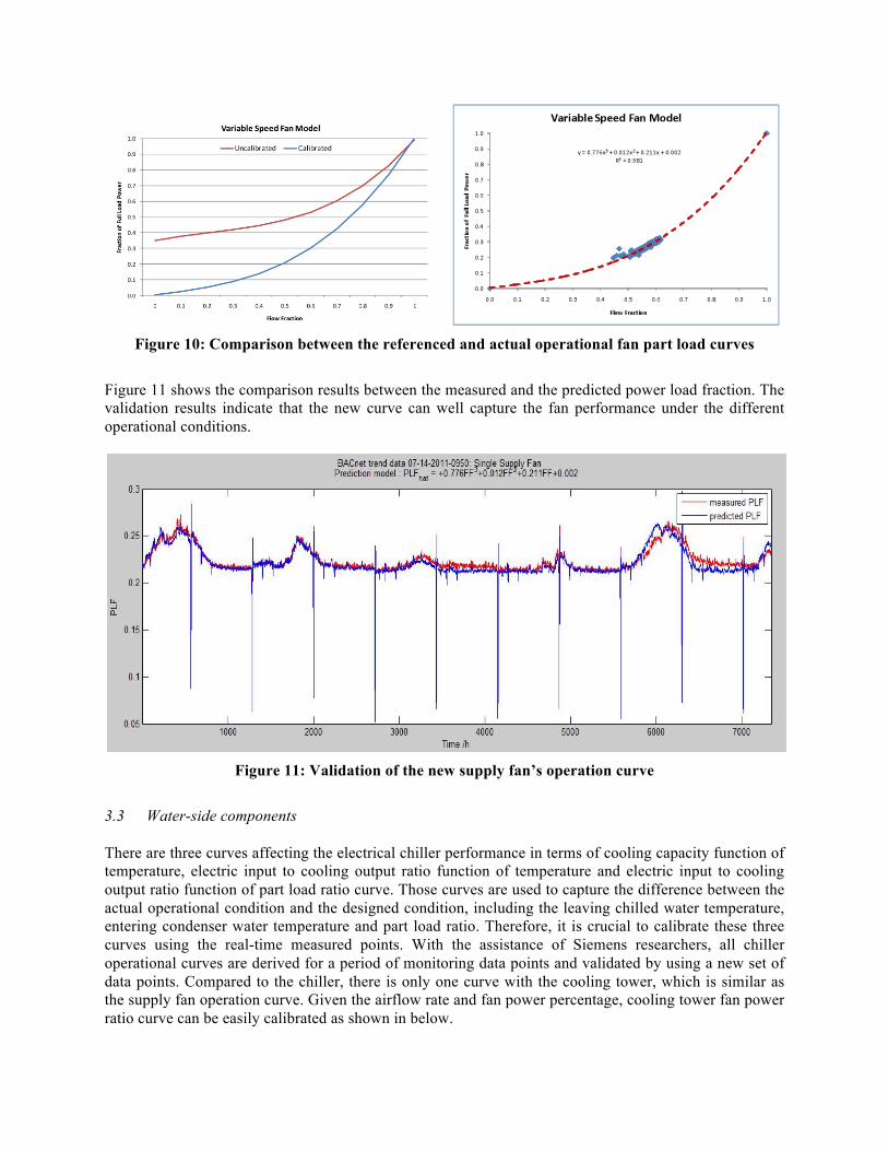
Figure 10: Comparison between the referenced and actual operational fan part load curves

Figure 11 shows the comparison results between the measured and the predicted power load fraction. The validation results indicate that the new curve can well capture the fan performance under the different operational conditions.

Figure 11: Validation of the new supply fan’s operation curve

3.3 Water-side components There are three curves affecting the electrical chiller performance in terms of cooling capacity function of temperature, electric input to cooling output ratio function of temperature and electric input to cooling output ratio function of part load ratio curve. Those curves are used to capture the difference between the actual operational condition and the designed condition, including the leaving chilled water temperature, entering condenser water temperature and part load ratio. Therefore, it is crucial to calibrate these three curves using the real-time measured points. With the assistance of Siemens researchers, all chiller operational curves are derived for a period of monitoring data points and validated by using a new set of data points. Compared to the chiller, there is only one curve with the cooling tower, which is similar as the supply fan operation curve. Given the airflow rate and fan power percentage, cooling tower fan power ratio curve can be easily calibrated as shown in below.

Figure 12: Electric Input to Cooling Output Ratio Function of Part Load Ratio Curve

Figure 13: Cooling Tower Fan Power Ratio as Function of Air Flow Ratio

4 Results 4.1 Whole building electrical power usage Due to the missing monitoring periods on sMAP, firstly 4 months of dataset in 2010 are used to compare the measured and simulated results at the whole building power usage level. The comparison between calibrated simulation and the measured results yields monthly mean bias error (MBE) within 10%. Taking a new dataset to evaluate the model prediction at the hourly level, it can be seen that the hourly simulation

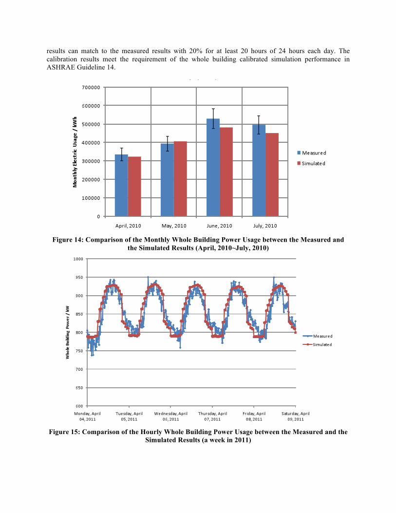
results can match to the measured results with 20% for at least 20 hours of 24 hours each day. The calibration results meet the requirement of the whole building calibrated simulation performance in ASHRAE Guideline 14.

Figure 14: Comparison of the Monthly Whole Building Power Usage between the Measured and

the Simulated Results (April, 2010~July, 2010)

Figure 15: Comparison of the Hourly Whole Building Power Usage between the Measured and the

Simulated Results (a week in 2011)

4.2 Calibration of Building System Components The use of the calibrated fan model curve, substantially improves the accuracy of the simulated fan power as compared to measured data. Figure 16 shows how the calibrated supply fan power matches with measured data.

Figure 16: Calibrated versus Uncalibrated Supply Fan Power Comparison with the Measured Data

Calibrated lighting and plug load model substantially matches measured lighting and plug load behavior in Figure 17. Additional submetering to disaggregate lighting and plugs could further increase model accuracy.

Figure 17: Measured, Calibrated and Uncalibrated Lighting and Plug Loads

The results were significant. In initial tests¸ the accuracy of an EnergyPlus model increased for the Variable Air Volume Fan system by over 15 times (1539%) and six times (594%) for the lighting and plug loads. Due to these and other measures, the overall whole building model error was improved by over four times (443%). In addition, the ability to forecast sheds during demand response event improved by a factor of 10 (1079%).

Table 3: Results of Monitoring Data based Model Calibration Methodology

Electric Load Uncalibrated model error (%MBE)

Calibrated model error (%MBE)

HVAC, VAV Fan (normal operation) 62.3 3.8

HVAC, VAV Fan (DR Event) 66.0 5.6

Lighting & Plugs 62.2 8.8

Whole Building 12.5 2.3

4.3 Model Prediction of Dynamic Response As discussed above, the calibrated model can match to the measured building performance at the whole building and sub-utility system component level with a good agreement. However, there is another challenge in predicting the effect of dynamic response control strategies on major system components including supply & return fans serving the whole office-side building. A demand response event was called at this facility on August 22nd, 2011. A set of DR strategies were tested between 2 pm and 7:30 pm. The selection of strategies (N. Motegi, 2007) depended on a) strategies

that were not yet simulated (supply air temperature increase); b) strategies that were already considered (global temperature adjustment); c) strategies that the simulation model could not replicate (disabling the reheat coil slowly). First, at 2 pm, supply air temperature was increased 2°F from 56°F to 58°F. An hour later, another 2°F supply air temperature increase was made. An hour later, all VAV boxes were controlled to provide ASHRAE default ventilation rates, which were 30% lower than the normal ventilation rates in the building. At 4:40pm, zone temperature setpoints were increased by 4°F from 70°F to 74°F. At 6:30pm, the reheat coil was disabled in the actual building. Finally at 7:30, all systems were reverted back to their normal operations slowly, over one hour period. The table below shows the actual strategies and simulated strategies tested on that date.

Table 4: Field Tested and Simulated Control Strategies on August 22nd, 2011

Time Control Points Field Test Control Strategies Time Simulated Control Strategies 2:07 Supply air temp Set to 58°F 2:00 Set to 58°F 3:02 Supply air temp Set to 60°F 3:00 Set to 60°F 3:56 Minimum air flow 70% of original value for all

VAVs 4:00 70% of original value for all

VAVs 4:40 Zone temp setpoints Increase by 4°F 4:40 Increase by 4°F 6:30 Reheat coil Disable 6:30 Disable 7:30 All Revert slowly 7:30 Revert immediately

The only strategy that was not implemented at the time this simulation model was developed was locking the reheat coil. Figure 18 shows the measured, calibrated and uncalibrated models at a DR test event. Calibrated model is presented with 10% error bars for visual comparison of the data. Information collected during the demand response event and comparison of simulated and measured data is especially valuable because the building systems are forced to operate outside of their normal operations thus, allowing the collection of extra data to evaluate the performance of the simulation model and facilitate its further calibration. In this case, we were able to collect more data on the flow rate of the VAV system and use these data to better calibrate the VAV system model.

Figure 18: Comparison of Supply Fan Power between the Measured and Simulated Results at a DR

Test Event

5 Conclusions and recommendations This paper demonstrates a case study of model development and monitoring data based model calibration for an existing office building. Given the purpose of the demand response control, the model was calibrated at a component level including building HVAC, lighting and plug loads.

• Identify the key factors with the model including local weather data, internal loads (occupant, lighting and plug loads), HVAC system components’ actual setpoints, control logics, operational curves.

• With the installation of sub-meters and sensors, more information has become available for the model calibration. The designed load densities and schedules were validated from the monitoring submetered lighting and plug loads at sub-floor level. The real operational curves were derived for supply & return fans, chiller and cooling towers.

• The comparison between the measured and simulated results at the whole building level yielded average MBE of 2.3%. At the system component level, the prediction of fan and lighting & plug load can achieve average MBEs of 3.3% and 8.8%, respectively.

• A field test of demand response control strategies was deployed to evaluate the dynamic response effect of the model prediction. It was found that the prediction of fan at a DR test mode yielded an average MBE of 5.6%.

• Based on the experience of model development and calibration, a scheme of automated model calibration was created to reduce the effort of manually adjustment of model inputs and improve the accuracy by bridging the sMAP and EnergyPlus model directly.

6 Acknowledgement This work described in this paper was coordinated by the University of California at Berkeley, Siemens Corporation Research and Demand Response Research Center and was funded by by the U.S. Department of Energy. The authors are grateful for the extensive support from the Auto-DR program managed by Demand Response Research Center at LBNL. Special thanks to David Culler, David Auslander, Therese Peffer for providing their insights and support, and Jianmin Zhu from Siemens Corporate Research. Thanks also to the building manager Domenico Caramagno from UC Berkeley for providing technical support. 7 References sMAP, Simple Measurement and Actuation Profile. http://new.openbms.org/ R. Yin, P. Xu, M. A. Piette, and S. Kiliccote, “Study on Auto-DR and pre-cooling of commercial buildings with thermal mass in California,” Energy and Buildings, vol. 42, no. 7, pp. 967–975, Jul. 2010. L. Wang, S. Greenberg, J. Fiegel, A. Rubalcava, S. Earni, X. Pang, R. Yin, S. Woodworth, and J. Hernandez-Maldonado, “Monitoring-based HVAC commissioning of an existing office building for energy efficiency,” Applied Energy, vol. 102, no. 0, pp. 1382–1390, Feb. 2013. P. Raftery, M. Keane, and J. O’Donnell, “Calibrating whole building energy models: An evidence-based methodology,” Energy and Buildings, vol. 43, no. 9, pp. 2356–2364, Sep. 2011. P. Raftery, M. Keane, and A. Costa, “Calibrating whole building energy models: Detailed case study using hourly measured data,” Energy and Buildings, vol. 43, no. 12, pp. 3666–3679, Dec. 2011 Title 24, 2005 Building Energy Efficiency Standards for Residential and Non Residential Buildings, California Energy Commission, 2005. N. Motegi, M.A. Piette, D. S. Watson, S. Kiliccote, P. Xu, Introduction to commercial building control strategies and technologies for demand response, LBNL-59975, 2007 ASHRAE, ANSI/ASHRAE 62.1-2010 Ventilation for Acceptable Indoor Air Quality. Atlanta, GA, American Society of Heating, Refrigeration and Air Conditioning Engineers, 2002 ASHRAE, ASHRAE guideline 14 for measurement of energy and demand savings. Atlanta, GA, American Society of Heating, Refrigeration and Air Conditioning Engineers, 2002