ilable at ScienceDirect

Atmospheric Environment 42 (2008) 8661–8673

Contents lists ava

Atmospheric Environment

journal homepage: www.elsevier .com/locate/atmosenv

Identification of factors affecting air pollution by dust aerosolPM10 in Brno City, Czech Republic

Zuzana Hrdlickova a,*, Jaroslav Michalek a, Miroslav Kolar b, Vıtezslav Vesely c

a Institute of Mathematics, Faculty of Mechanical Engineering, Brno University of Technology, Technicka 2896/2, 616 69 Brno, Czech Republicb Department of Geography, Faculty of Science, Masaryk University, Kotlarska 2, 611 37 Brno, Czech Republicc Department of Applied Mathematics and Computer Science, Faculty of Economics and Administration, Masaryk University, Lipova 41a, 602 00 Brno,Czech Republic

a r t i c l e i n f o

Article history:Received 22 February 2008Received in revised form 8 August 2008Accepted 8 August 2008

Keywords:Dust aerosol PM10

Generalized autoregressive linear modelGamma distributionGoodness-of-fit statisticAnscombe residual

* Corresponding author. Tel.: þ420 541 142 532; faE-mail addresses: hrdlickova.z@fme.vutbr.cz (Z. H

@fme.vutbr.cz (J. Michalek), kolar@sci.muni.cz (M.muni.cz (V. Vesely).

1352-2310/$ – see front matter � 2008 Elsevier Ltddoi:10.1016/j.atmosenv.2008.08.017

a b s t r a c t

The statistical analysis of the observation of dust aerosol PM10 from four monitoringstations of the agglomeration of the city of Brno during a time period from January 1, 1998until December 30, 2005 is presented. The main meteorological factors affecting airpollution at each station were identified by means of a generalized autoregressive linearmodel with gamma distribution of the response variable and log-link function. Along withmeteorological factors, the influence of the heating season and weekdays on the airpollution was considered. The suggested model can be used for a prediction of the dailymean value of dust aerosol PM10 at a given station using selected factors and their previousvalues.

� 2008 Elsevier Ltd. All rights reserved.

1. Introduction

Quality of the air is one of the basic indicators of theoverall quality of the environment. Air pollution hasbecome a local as well as a regional issue of big cities,industrial centers and surroundings of transport routes,especially roads and highways. Nevertheless the release ofprimarily harmless substances fundamentally affectsproperties of the atmosphere (such as greenhouse gases orFreon) with global repercussions. The focus of this article isan evaluation of air pollution with dust aerosol in the city ofBrno, the second largest city of the Czech Republic, basedon data on the occurrence of the pollutants and meteoro-logical data. The purpose is to describe and rationalizetransformations of the pollution of the air of the Brnoagglomeration in time and space to identify the causes ofthe current status and to predict significant exceeding of

x: þ420 541 142 710.rdlickova), michalekKolar), vesely@econ.

. All rights reserved.

the hygienic limits. When the hygienic limits are surpassed,this information enters the crisis management system andappropriate measures are taken. This is one of the reasonsof the implementation of the long-term research project ofthe Ministry of Education, Youth and Sports of the CzechRepublic no. MSM0021622418 entitled ‘‘Dynamic Geo-visualization in Crisis Management’’, in the context ofwhich the present article has been written. Preliminaryresults of the research were presented at Hrdlickova et al.(2006).

Dust aerosol comprises of all particles in the air that arenot gaseous, including: molecular clusters, ice crystals,various solid particles (metal particles, silicates, fluorides,oxides, nitrates, chlorides, sulphates, etc.), drops of liquids,pollen, small insects, etc. The decisive quantities of dustaerosol are represented by particles smaller than 1 mm,mostly originating from condensation and coagulation.Particles larger than 1 mm are usually primarily emitted.Most frequently, the dust fractions of particles of size below10 mm (PM10), 5 mm (PM5) and 2.5 mm (PM2.5) are analyzed.Dust aerosol for the purpose of this article mean PM10

fraction size.

Table 1Activity of heating plants in the Czech Republic

Month Jan Feb Mar Apr May Jun–Aug Sep Oct Nov Dec

HS 0.19 0.16 0.14 0.09 0.02 0 0.01 0.08 0.14 0.17

Z. Hrdlickova et al. / Atmospheric Environment 42 (2008) 8661–86738662

A large number of recent epidemiological studies haveobserved a negative impact of ambient particle concen-trations on human health including increases in respira-tory symptoms and diseases (Franchini and Mannucci,2007), hospital and emergency department admissions(Chen et al., 2007) and mortality (Qian et al., 2007). InEuropean Union, the Council Directive (1996/62/EC) onambient air quality assessment and management estab-lishes the basic principles of a common strategy to defineand set objectives for ambient air quality in order to avoid,prevent or reduce harmful effects on human health andthe environment, assess ambient air quality in theMember States, inform the public, notably by means ofalert thresholds, and improve air quality where it isunsatisfactory. According to the follow-up Council Direc-tive (1999/30/EC) the limit value for the daily PM10

average is 50 mg m�3 and should not to be exceeded morethan 35 times a calendar year and the limit value for theannual PM10 average is 40 mg m�3 since January 1, 2005.However, PM10 limit values are currently being exceededin more than 370 zones – see Press Release (MEMO/07/

Win

d

Directio

n

1/011/001/991/98

360270180900

Win

d

Velo

city

1/011/001/991/98

10

5

0

Relative

Hu

mid

ity

1/011/001/991/98

1007550250

Tem

peratu

re

1/011/001/991/98

3020100-10

Du

st

Aero

so

l

1/011/001/991/98

300

200

100

0

Fig. 1. Values of meteorological elements and concentrations of dust aerosol in theasterisk on the x axis.

571). At the studied stations in Brno (see Section 2), thedaily PM10 limit was exceeded on 8% (2004) to 85% (2002)of the yearly measurements. The annual average of theavailable PM10 values varied from 30 mg m�3 (2004) to72 mg m�3 (2002). The summer PM10 averages weremostly lower than those for the winter months with thelargest difference of 23 mg m�3. Correspondingly, theexceedances of the limit were observed in the wintermonths more frequently (an average of 59%).

Anthropogenic sources of dust aerosol include powergeneration, metallurgy (especially foundries), ore mining,manufacture of construction materials and civil industry.Another currently relevant secondary source of dustaerosol is transport mostly affecting urban areas andcities. Transport multiplies pollution from other sources –dispersion of transported materials, industrial transport,etc. This source of dust aerosol has a number of specificsthat worsen the impact of the pollution. The transportnot only produces new dust aerosol, but also stirspreviously settled dust, emits pollutants close to humansand biota and produces trace quantities of toxicsubstances, that bound to the dust particles. Spread ofemissions to the surroundings of their source andtherefore the emission conditions depend on four groupsof factors: parameters of the source (capacity, variabilityin time, height above ground, temperature, output speedof emissions), properties of the emissions, effect of earth

1/061/051/041/031/02

1/061/051/041/031/02

1/061/051/041/031/02

1/061/051/041/031/02

1/061/051/041/031/02

period 1998–2005 at Arboretum station. Extreme values are marked with an

Z. Hrdlickova et al. / Atmospheric Environment 42 (2008) 8661–8673 8663

surface and meteorological factors. The latter generallyexercise a decisive effect on the spread of pollutants.Meteorological factors can be divided into factors withdirect effect (velocity and direction of air flow, thermalstratification of atmosphere close to the earth surface,atmospheric precipitation) and factors with indirecteffect (temperature, sunshine, air humidity, cloudformation, air pressure). The indirect effect factors affectthe nature of the direct effect ones.

2. Data

The performed analysis is based on data from fourmonitoring stations of the agglomeration of the city ofBrno, namely Arboretum, Bohunice, Zidenice and Zvo-narka. The time period of monitoring was from January 1,1998 until December 30, 2005. Together with dust aero-sol Apt [mg m�3] the factors wind velocity Vt [m s�1],wind direction Dt [�], air temperature Tt [�C] and relativeair humidity Ht [%] were measured to evaluate the effectsof meteorological conditions on the emission situation ateach monitoring station. The data used in the analysis aredaily means of half-an-hour measurements of monitoredfactors and the subscript t stands for a day.

It is well known that the level of dust aerosol issignificantly higher in heating season and its values onthe weekdays differ from weekend values – see model in

Win

d

Directio

n

360270180900

Win

d

Velo

city

10

5

0

Relative

Hu

mid

ity

1007550250

3020100-10

Du

st

Aero

so

l

300

200

100

011/011/001/991/98

11/011/001/991/98

11/011/001/991/98

11/011/001/991/98

11/011/001/991/98

Tem

peratu

re

Fig. 2. Values of meteorological elements and concentrations of dust aerosol in theasterisk on the x axis.

Hormann et al. (2005). To involve the heating plantactivity, an additional variable heating season HSt wasintroduced. The values of variable HSt vary acrossmonths in compliance with the Czech GovernmentDecree no. 372/2001 Coll. as given in Table 1. Anotherexplanatory binary variable is weekend Ft with the valueof 1 on Saturdays and Sundays and 0 for the rest of theweek. Note, that a model with two separate binaryvariables for Saturdays and Sundays was considered inthe first step. However, the procedure for choosing thebest submodel described in Section 4 rarely showedsuch a model to be irreducible to a model with variableFt in contrast to the model described in Chaloulakouet al. (2003).

Flow charts of values of the measured variablesacross the period in question are in Figs. 1–4. As can beseen from the graphic representations of the time seriesfor the individual stations the development of the Apt

series in monitored period is strongly non-stationary andthere are considerable changes in the series courses.Data contain sequences of missing values of either Apt orthe measured covariates. The time series also includenon-proportionately low or high values of dust forma-tion evaluated by experts as incorrect measurements(Apt < 2 mg m�3, Apt > 400 mg m�3). The time of occur-rence of these values can be seen in Figs. 1–4. Thesevalues were excluded from the further analysis.

1/061/051/041/03/02

1/061/051/041/03/02

1/061/051/041/03/02

1/061/051/041/03/02

1/061/051/041/03/02

period 1998–2005 at Zidenice station. Extreme values are marked with an

Win

d

Directio

n

360270180900

Win

d

Velo

city

10

5

0

Relative

Hu

mid

ity

1007550250

Tem

peratu

re 30

20100-10

Du

st

Aero

so

l

300

200

100

01/061/051/041/031/021/011/001/991/98

1/061/051/041/031/021/011/001/991/98

1/061/051/041/031/021/011/001/991/98

1/061/051/041/031/021/011/001/991/98

1/061/051/041/031/021/011/001/991/98

Fig. 3. Values of meteorological elements and concentrations of dust aerosol in the period 1998–2005 at Bohunice station. Extreme values are marked with anasterisk on the x axis.

Z. Hrdlickova et al. / Atmospheric Environment 42 (2008) 8661–86738664

2.1. Description of localities of pollution measurement

Satellite maps used to describe the location of thestudied monitoring stations were downloaded from http://www.mapy.cz on April 3, 2006.

Arboretum is a station located in the botanical garden ofMendel University of Agriculture and Forestry (see Fig. 5).Close by there is a heavy-traffic intersection. The station issituated on the top of a hill. North of the station there aremilitary barracks, south of the station there is the campusof Mendel University of Agriculture and Forestry, east of thestation there is a residential housing and west of the stationthere is the botanical garden (arboretum). On the westernslope of the hill there is another heavy-traffic intersection,industrial plants (heating plant) and also unused landwithout greenery. The station is surrounded with areas ofreduced humidity.

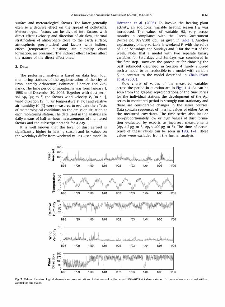
Zidenice station is situated by the boundary of thebarrack premises near the heavy-traffic Svatoplukovastreet, from which it is shielded with an about 3 m highwall (see Fig. 6). North of the station there are warehouses,small manufacturing plants and a railway line. East of thestation there is a military barracks and west of the stationthere is a residential housing. South of the station there isan intersection with Rokytova street and more residential

houses. The station is situated in the Svitava river valleyand is surrounded with areas of reduced humidity.

Bohunice is a station located near the Lany street on thesouthern edge of the Bohunice housing estate (see Fig. 7).The station is protected against effects of the traffic in theLany street with two rows of houses and grown up vege-tation. North of the station there is the Bohunice housingestate. South of the station there are gardens, the campus ofthe Secondary Gardening School and behind it there isa railway line and D1 highway (350 m from the station).Characteristic features of this area include relatively largestretches of unused fields. The station is located ona moderate south-oriented slope. The locality is sur-rounded with reduced humidity areas. There is increasedchance of dynamic turbulences around the station.

Zvonarka station is installed by the heavy-traffic Opus-tena street in an area heavily loaded with traffic andmanufacturing plants (see Fig. 8). North of the station thereis the Vankovka center, the repair plant of the bus terminal.West of the station there is a stretch of land so far unused.South and east of the station there is a parking lot and theZvonarka bus station. Farther away there is the train stationfor goods and more heavy-traffic roads. The station is sit-uated in the Svratka river valley and is surrounded withareas of reduced humidity.

Win

d

Directio

n

360270180900

Win

d

Velo

city

10

5

0

Relative

Hu

mid

ity

1007550250

Tem

peratu

re 30

20100-10

Du

st

Aero

so

l

300

200

100

01/061/051/041/031/021/011/001/991/98

1/061/051/041/031/021/011/001/991/98

1/061/051/041/031/021/011/001/991/98

1/061/051/041/031/021/011/001/991/98

1/061/051/041/031/021/011/001/991/98

Fig. 4. Values of meteorological elements and concentrations of dust aerosol in the period 1998–2005 at Zvonarka station. Extreme values are marked with anasterisk on the x axis.

Z. Hrdlickova et al. / Atmospheric Environment 42 (2008) 8661–8673 8665

As can be seen from the graphic representations of thetime series for the individual stations in Figs. 1–4 the prog-ress of the dust formation within the inspected period waschanging considerably. The main cause of the change in June2003, clearly seen at Arboretum and Zidenice stations, wasa reduction of emissions coming from the peak sources – the

Fig. 5. Position of Arboretum station. Two long white arrows indicate wind directionby the presented model. Solid and dashed line represent estimated wind direction

heating plants Brno-North and �Cerveny Mlyn – and a trafficrelieve of the locality by the Arboretum station caused by anopening of the Husovice tunnel. For that reason the timelines of the Arboretum and the Zidenice stations weredivided into two sections, from January 1,1998 until May 31,2003 and from June 1, 2003 until December 31, 2005. For the

s of maximum pollutant concentration oriented to the station and estimatedfor the first (76�) and the second (88�) time section, respectively.

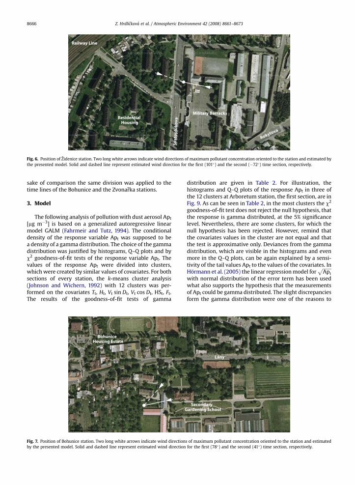
Fig. 6. Position of Zidenice station. Two long white arrows indicate wind directions of maximum pollutant concentration oriented to the station and estimated bythe presented model. Solid and dashed line represent estimated wind direction for the first (101�) and the second (�72�) time section, respectively.

Z. Hrdlickova et al. / Atmospheric Environment 42 (2008) 8661–86738666

sake of comparison the same division was applied to thetime lines of the Bohunice and the Zvonarka stations.

3. Model

The following analysis of pollution with dust aerosol Apt

[mg m�3] is based on a generalized autoregressive linearmodel GALM (Fahrmeir and Tutz, 1994). The conditionaldensity of the response variable Apt was supposed to bea density of a gamma distribution. The choice of the gammadistribution was justified by histograms, Q–Q plots and byc2 goodness-of-fit tests of the response variable Apt. Thevalues of the response Apt were divided into clusters,which were created by similar values of covariates. For bothsections of every station, the k-means cluster analysis(Johnson and Wichern, 1992) with 12 clusters was per-formed on the covariates Tt, Ht, Vt sin Dt, Vt cos Dt, HSt, Ft.The results of the goodness-of-fit tests of gamma

Fig. 7. Position of Bohunice station. Two long white arrows indicate wind directionby the presented model. Solid and dashed line represent estimated wind direction

distribution are given in Table 2. For illustration, thehistograms and Q–Q plots of the response Apt in three ofthe 12 clusters at Arboretum station, the first section, are inFig. 9. As can be seen in Table 2, in the most clusters the c2

goodness-of-fit test does not reject the null hypothesis, thatthe response is gamma distributed, at the 5% significancelevel. Nevertheless, there are some clusters, for which thenull hypothesis has been rejected. However, remind thatthe covariates values in the cluster are not equal and thatthe test is approximative only. Deviances from the gammadistribution, which are visible in the histograms and evenmore in the Q–Q plots, can be again explained by a sensi-tivity of the tail values Apt to the values of the covariates. InHormann et al. (2005) the linear regression model for

ffiffiffiffiffiffiffiffiApt

pwith normal distribution of the error term has been usedwhat also supports the hypothesis that the measurementsof Apt could be gamma distributed. The slight discrepanciesform the gamma distribution were one of the reasons to

s of maximum pollutant concentration oriented to the station and estimatedfor the first (78�) and the second (41�) time section, respectively.

Fig. 8. Position of Zvonarka station. Two long white arrows indicate wind directions of maximum pollutant concentration oriented to the station and estimatedby the presented model. Solid and dashed line represent estimated wind direction for the first (101�) and the second (92�) time section, respectively.

Z. Hrdlickova et al. / Atmospheric Environment 42 (2008) 8661–8673 8667

consider a non-canonical link in the GALM as described inthe next paragraph.

Gamma distribution is a member of the exponentialclass and thus the GALM can be considered. The canonicallink function for the gamma distribution is the reciprocalfunction. Another important link function for gammadistribution is the log-link function – see Fahrmeir and Tutz(1994, p. 23). The log-link can be used to improve the fit,when the distribution of the response variable showsdiscrepancies from the gamma distribution in the tails, aswas seen in Fig. 9. Note that in Li et al. (1999) the logarithm

Table 2Results for c2 goodness-of-fit tests of gamma distribution of Apt in clusters C1, .

Vt sin Dt, Vt cos Dt, HSt, Ft

Arboretum Zidenice

Section 1 Section 2 Section 1 Section 2

C1 4.585 1.925 4.069 2.668(75) (70) (96) (30)

C2 0.519 8.955 3.749 2.179(144) (115) (92) (37)

C3 6.639 16.532* 0.230 4.062(168) (97) (106) (65)

C4 3.488 19.157** 5.757 5.259(174) (66) (103) (79)

C5 7.655 6.609 9.581 6.372(145) (86) (130) (103)

C6 13.200* 3.209 1.091 9.616*(233) (101) (70) (53)

C7 10.653 6.778 0.013 6.365(125) (87) (28) (83)

C8 2.736 3.315 4.450 2.779(183) (44) (140) (111)

C9 2.176 1.663 2.260 3.941(162) (45) (42) (41)

C10 7.145 2.980 6.457 3.979(94) (42) (128) (74)

C11 8.924 2.724 5.801 4.685(126) (57) (132) (74)

C12 26.719*** 0.431 1.915 2.443(197) (92) (76) (53)

Each cell consists of observed test statistic and size of cluster (in parentheses). A

transformation of the hourly PM10 was chosen for makingthe frequency distribution of the response variable in thespatial-temporal model of PM10 in Vancouver approxi-mately normal. The log-transformed daily average PM10

concentration values were also considered as responses inthe regression models in Chaloulakou et al. (2003). Thecanonical link and the log-link have been used in thefurther analysis.

Before a model description, it is necessary to choosecovariates for a linear predictor. In the first place the winddirection Dt, measured as an oriented angle between the

, C12 identified by k-means cluster analysis performed on covariates Tt, Ht,

Bohunice Zvonarka

Section 1 Section 2 Section 1 Section 2

10.447 2.994 5.989 10.034*(155) (91) (177) (63)10.623 3.361 1.316 3.540(140) (59) (104) (53)6.230 5.049 3.447 2.420(136) (41) (95) (39)8.062 9.471 7.933 4.142(114) (84) (138) (59)5.549 4.837 2.202 2.745(79) (40) (139) (52)5.644 5.764 5.967 1.244(60) (87) (118) (96)10.208 19.367** 1.121 4.854(188) (115) (167) (79)4.408 3.465 1.830 0.110(138) (76) (99) (14)3.303 3.902 20.071** 1.229(113) (68) (148) (53)7.446 5.580 8.584 6.872(149) (55) (92) (117)2.810 30.006*** 3.421 9.570(64) (126) (168) (107)3.339 13.452*** 6.392 9.170(137) (56) (221) (96)

sterisks indicate p-value of the test (*p < 0.05, **p < 0.01, ***p < 0.001).

Cluster 3

Pollution with dust aerosol [µg.m−3

]

Nu

mb

er o

f o

bs

erv

atio

ns

20016012080400

70

60

50

40

30

20

10

0

Cluster 3

Theoretical Quantiles

Em

pirical Q

uan

tiles

1801501209060300

180

150

120

90

60

30

0

Cluster 10

Pollution with dust aerosol [µg.m−3

]

Nu

mb

er o

f o

bservatio

ns

16012080400

30

20

10

0

Cluster 10

Theoretical Quantiles

Em

pirical Q

uan

tiles

200150100500

200

150

100

50

0

Cluster 12

Nu

mb

er o

f o

bs

erv

atio

ns

1501251007550250

100

75

50

25

0

Pollution with dust aerosol [µg.m−3

]

Cluster 12

Theoretical Quantiles

Em

pirical Q

ua

ntile

s

16012080400

160

120

80

40

0

Fig. 9. Histograms with fitted probability density functions of gamma distribution and Q–Q plots for the response Apt in three of 12 clusters identified by k-meanscluster analysis performed on covariates Tt, Ht, Vt sin Dt, Vt cos Dt, HSt, Ft for Arboretum station, the first section. Clusters were chosen to illustrate different results –good fit in Cluster 3 (c2 ¼ 6.639, df ¼ 5), medium fit in Cluster 10 (c2 ¼ 7.145, df ¼ 6) and worse fit in Cluster 12 (c2 ¼ 26.719***, df ¼ 4).

Z. Hrdlickova et al. / Atmospheric Environment 42 (2008) 8661–86738668

vector pointing north of the station and the observed winddirection vector pointing to the station, has a circulardistribution and thus it is not suitable to be considered asa covariate for the linear predictor directly. For the sake ofinterpretation the wind velocity Vt should not be consid-ered separately from the wind direction Dt. Therefore theprojections Vt sin Dt and Vt cos Dt are included in themodel. Similarly to Somerville et al. (1996), reparametri-zation of the linear predictor with Vt sin Dt and Vt cos Dt

provides an estimate of the angle S [�] between the vectorpointing north of the station and the vector pointing fromthe direction of maximum pollutant concentration to thestation. Details on this reparametrization are given later inthis section.

If significant, one or more relevant angles S can also beidentified by the method of overcomplete frames (Chen et al.,1998; Vesely and Tonner, 2006). Such an approach to the datastudied in this paper was applied in Vesely et al. (2006).

Then the covariates chosen for our GALM model were Ht,Vt sin Dt, Vt cos Dt together with the categorical covariates

Table 3Comparison of GALM with canonical link (M1) and GALM with log-link (M2) by

Arboretum Zidenice

Section 1 Section 2 Section 1 Section

D in M1 199.008 61.558 75.205 69.088D in M2 192.365 61.828 72.036 65.865

cans2 in M1 197.213 61.165 74.784 67.957

cans2 in M2 190.626 61.444 71.645 64.918

HSt, Ft. Furthermore the autoregressive variables with lagone Apt � 1, Ht � 1 were included. For the model with log-link function the variable ln(Apt � 1) was involved instead ofApt � 1. Variable HSt clearly reflects the mean trend of the airtemperature Tt. Therefore to eliminate a co-linearity in themodel the air temperature gradient (Tt � Tt � 1) instead oftwo separate covariates Tt and Tt � 1 was chosen for themodel. Then the considered GALM with log-link function isexpressed by an equation

lnðmtÞ ¼ b0 þ b1 lnðApt�1Þ þ b2ðTt � Tt�1Þ þ b3Ht=100

þ b4Vt sin Dt þ b5Vt cos Dt þ b6Ht�1=100

þ b7HSt þ b8Ft; ð1Þ

where

� b0; . ; b8 are unknown parameters which have to beestimated,� mt ¼ EðAptjStÞ stands for the conditional expectationof the response variable, here St is the set of variables

deviance D and Pearson c2 statistics for Anscombe residuals cans2

Bohunice Zvonarka

2 Section 1 Section 2 Section 1 Section 2

114.908 77.812 148.128 46.653109.490 75.525 137.099 45.484

114.190 77.254 147.211 46.489108.802 74.848 136.267 45.323

Table 4Parameter estimates together with their standard deviation (in parentheses) for the model (1)

Arboretum Zidenice Bohunice Zvonarka

Section 1 Section 2 Section 1 Section 2 Section 1 Section 2 Section 1 Section 2

const. 2.079 (0.091) 1.772 (0.115) 2.086 (0.117) 2.715 (0.196) 1.799 (0.097) 1.535 (0.153) 2.181 (0.092) 2.359 (0.133)ln(Apt � 1) 0.603 (0.018) 0.579 (0.027) 0.579 (0.023) 0.457 (0.036) 0.592 (0.021) 0.718 (0.027) 0.545 (0.020) 0.477 (0.030)Tt � Tt � 1 0.014 (0.004) 0.008 (0.004) 0.020 (0.006) 0.007 (0.003) 0.024 (0.006) 0.010 (0.004) 0.010 (0.004)Ht/100 �0.585 (0.070) �0.436 (0.084) �0.459 (0.070) �0.905 (0.129) �0.443 (0.062) �0.465 (0.076)Vt sin Dt 0.090 (0.009) 0.077 (0.013) 0.049 (0.020) �0.089 (0.052) 0.058 (0.005) 0.038 (0.016) 0.051 (0.007) 0.056 (0.018)Vt cos Dt 0.023 (0.009) 0.002 (0.021) �0.010 (0.012) 0.029 (0.018) 0.012 (0.006) 0.045 (0.030) �0.010 (0.008) �0.001 (0.029)Ht � 1/100 �0.304 (0.069) �0.523 (0.125)HSt 0.938 (0.122) 1.045 (0.155) 0.617 (0.122) 2.021 (0.219) 1.107 (0.124) 0.945 (0.202) 1.306 (0.120) 1.373 (0.151)Ft �0.125 (0.018) �0.128 (0.021) �0.147 (0.017) �0.225 (0.028) �0.038 (0.017) �0.102 (0.028) �0.163 (0.016) �0.125 (0.019)

b45 0.093 0.077 0.050 0.093 0.060 0.059 0.052 0.056S 76� 88� 101� �72� 78� 41� 101� 92�

D 192.365 61.828 72.036 65.865 109.490 85.565 137.099 45.484cans

2 190.626 61.444 71.645 64.918 108.802 84.418 136.267 45.323

W 0.006 6.245 1.658 0.003 2.973 0.694 3.630 0.000f 1805 892 1127 787 1459 885 1651 813n 1813 899 1135 795 1467 893 1659 821c0.95

2 3.841 5.991 3.841 3.841 3.841 3.841 3.841 3.841

The table is completed by estimated angle S which identify the direction of maximum pollutant concentration and recalculated regression parameter b45 atVt cos(Dt � S). Then goodness-of-fit statistics D, cans

2 and Wald statistic (W) together with their degrees of freedom (f), length of modeled time series (n) andcorresponding c0.95

2 quantile for each measured series follow.

Z. Hrdlickova et al. / Atmospheric Environment 42 (2008) 8661–8673 8669

used on the right-hand side of the model Eq. (1). Thus St

consists of the variables Tt � Tt � 1, Ht, Vt sin Dt, Vt cos Dt,Apt � 1, Ht � 1, HSt, Ft.

Covariate Ht/100 and Ht � 1/100 is considered instead ofHt and Ht � 1, respectively, to obtain estimates of the cor-responding regression parameters of an order similar to theorder of other regression parameters.

The component of the linear predictor

b4Vt sin Dt þ b5Vt cos Dt (2)

can be reparametrized by the sum formula tob45Vt cos(Dt � S), where b45 and S are unknown parametersand their estimates can be obtained from b4 and b5. Aspointed out in Somerville et al. (1996) S identifies an angleof the direction of maximum pollutant concentration.

An

sco

mb

e

Resid

uals 2

0

-2

Du

st A

ero

so

l Apt

1/98 1/99 1/00

1/98 1/99 1/00

300

200

100

0

Fig. 10. Observed and predicted values of dust aerosol Apt and correspondin

Because the GALM with log-link function performedbetter than GALM with canonical link on the given data theequation for GALM with canonical link is left. Hereinafterthe analysis concentrates on the model with log-link.

4. Parameter identifications and model verification

The parameters b0; . ; b8 of model (1) were estimatedby the maximum likelihood method (Fahrmeir and Tutz,1994) adapted for GALM with gamma conditionallydistributed response. Numerical calculations were imple-mented in MATLAB software package and the procedureglmfit from the Statistics Toolbox has been used for fittingthe model.

The choice of the best submodel of the studied modelwas performed by stepwise backward selection using Wald

1/01 1/02 1/03

1/01 1/02 1/03

g plot of Anscombe residuals at Arboretum station, the first section.

An

sc

om

be

Resid

uals 2

0

-2

Du

st A

ero

so

l Apt

6/03 1/04 1/05

6/03 1/04 1/05

300

200

100

0

Fig. 11. Observed and predicted values of dust aerosol Apt and corresponding plot of Anscombe residuals at Arboretum station, the second section.

Z. Hrdlickova et al. / Atmospheric Environment 42 (2008) 8661–86738670

statistic – see Fahrmeir and Tutz (1994, pp. 122–123). Thisway the variables in the submodel of the model (1) with thebest prediction ability were identified. Then the final bestsubmodel was tested against the maximal model usingWald statistic to verify, whether the best selected submodelis acceptable. The 5% significance level has been usedthroughout the analysis.

The model verification was based on the analysis ofresiduals and goodness-of-fit tests. The values mt wereestimated by bmt using the best submodel corresponding tothe model (1) with estimated parameters. Then theobserved values of Apt together with the estimated trend bmt

were plotted. Later the Anscombe residuals – see McCullaghand Nelder (1989), (Section 2.4.2) – were calculated andplotted. Further the Pearson c2 statistics for Anscomberesiduals given by

c2ans ¼ 9

Xn

i¼1

�Y1=3

i � bm1=3i

�2

bm2=3i

(3)

and deviance D given by

1/00 1/01

1/00 1/01

An

sc

om

be

Resid

uals 2

0

-2

Du

st A

ero

so

l Apt

300

200

100

0

Fig. 12. Observed and predicted values of dust aerosol Apt and correspond

D ¼ 2Xn �

� ln�

Yi=bmi

�þ�

Yi � bmi

�.bmi

�(4)

i¼1

were calculated to compare different models. The values ofthese two goodness-of-fit statistics enabled us to choosethe best model and led us to prefer GALM with log-link (1)to GALM with canonical link.

5. Results

First the GALMs with canonical link and log-link werecompared. Observed values of the goodness-of-fit statisticscans

2 (3) and D (4) for both models are given in Table 3. ForGALM with log-link, smaller values of the goodness-of-fitstatistics cans

2 and D were achieved in all cases except forthe second section at Arboretum station. Note that thisconclusion corresponds with the results in Vesely et al.(2007), where a forecasting ability was the main criterion.Therefore the GALM with log-link was examined further.

Table 4 includes parameter estimates and their stan-dard deviations for the selected best submodels. Finally,to assess the model suitability, measured values were

1/02 1/03

1/02 1/03

ing plot of Anscombe residuals at Zidenice station, the first section.

6/03 1/04 1/05

6/03 1/04 1/05

An

sco

mb

e

Resid

uals 2

0

-2

Du

st A

ero

so

l Apt

300

200

100

0

Fig. 13. Observed and predicted values of dust aerosol Apt and corresponding plot of Anscombe residuals at Zidenice station, the second section. Extremeobserved values (Apt > 300 mg m�3) and extreme residuals (Apt � bmt > 2 m g:m�3) are marked with plus (‘‘þ’’) at the bottom of the graph and asterisk (‘‘*’’) at thetop of the graph, respectively.

1/98 1/99 1/00 1/01 1/02 1/03

1/98 1/99 1/00 1/01 1/02 1/03

An

sco

mb

e

Resid

uals 2

0

-2

Du

st A

ero

so

l Apt

300

200

100

0

Fig. 14. Observed and predicted values of dust aerosol Apt and corresponding plot of Anscombe residuals at Bohunice station, the first section.

6/03 1/04 1/05

6/03 1/04 1/05

An

sco

mb

e

Resid

uals 2

0

-2

Du

st A

ero

so

l Apt

300

200

100

0

Fig. 15. Observed and predicted values of dust aerosol Apt and corresponding plot of Anscombe residuals at Bohunice station, the second section. Extremeresiduals (Apt � bmt > 2 m g:m�3) are marked with asterisks (‘‘*’’) at the top of the graph.

Z. Hrdlickova et al. / Atmospheric Environment 42 (2008) 8661–8673 8671

1/99 1/00 1/01 1/02 1/03

1/99 1/00 1/01 1/02 1/03

An

sco

mb

e

Resid

uals 2

0

-2

Du

st A

ero

so

l Apt

300

200

100

0

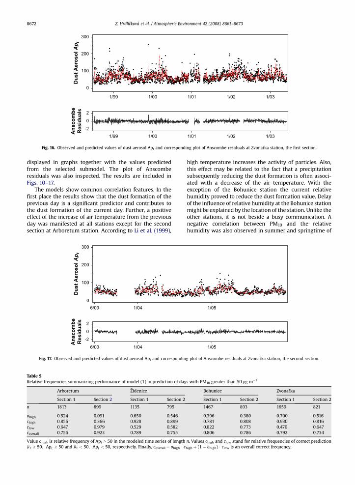
Fig. 16. Observed and predicted values of dust aerosol Apt and corresponding plot of Anscombe residuals at Zvonarka station, the first section.

Z. Hrdlickova et al. / Atmospheric Environment 42 (2008) 8661–86738672

displayed in graphs together with the values predictedfrom the selected submodel. The plot of Anscomberesiduals was also inspected. The results are included inFigs. 10–17.

The models show common correlation features. In thefirst place the results show that the dust formation of theprevious day is a significant predictor and contributes tothe dust formation of the current day. Further, a positiveeffect of the increase of air temperature from the previousday was manifested at all stations except for the secondsection at Arboretum station. According to Li et al. (1999),

6/03 1/04

6/03 1/04

An

sco

mb

e

Resid

uals 2

0

-2

Du

st A

ero

so

l Apt

300

200

100

0

Fig. 17. Observed and predicted values of dust aerosol Apt and correspondin

Table 5Relative frequencies summarizing performance of model (1) in prediction of day

Arboretum Zidenice

Section 1 Section 2 Section 1 Section 2

n 1813 899 1135 795

ohigh 0.524 0.091 0.650 0.546chigh 0.856 0.366 0.928 0.899clow 0.647 0.979 0.529 0.582coverall 0.756 0.923 0.789 0.755

Value ohigh is relative frequency of Apt � 50 in the modeled time series of lengthbmt � 50; Apt � 50 and bmt < 50; Apt < 50, respectively. Finally, coverall ¼ ohigh $ c

high temperature increases the activity of particles. Also,this effect may be related to the fact that a precipitationsubsequently reducing the dust formation is often associ-ated with a decrease of the air temperature. With theexception of the Bohunice station the current relativehumidity proved to reduce the dust formation value. Delayof the influence of relative humidity at the Bohunice stationmight be explained by the location of the station. Unlike theother stations, it is not beside a busy communication. Anegative correlation between PM10 and the relativehumidity was also observed in summer and springtime of

1/05

1/05

g plot of Anscombe residuals at Zvonarka station, the second section.

s with PM10 greater than 50 mg m�3

Bohunice Zvonarka

Section 1 Section 2 Section 1 Section 2

1467 893 1659 821

0.396 0.380 0.700 0.5160.781 0.808 0.930 0.8160.822 0.773 0.470 0.6470.806 0.786 0.792 0.734

n. Values chigh and clow stand for relative frequencies of correct prediction

high þ (1 � ohigh) $ clow is an overall correct frequency.

Z. Hrdlickova et al. / Atmospheric Environment 42 (2008) 8661–8673 8673

the period from 1999 until 2003 at some monitoring sitesin Egypt (Elminir, 2007). A positive effect of the heatingperiod manifested itself at all stations. Similarly to theresults of an analysis of PM10 in Vancouver conducted inLi et al. (1999), a negative effect of the weekend variablewas identically indicated at all stations.

As noted in Li et al. (1999) air movement may transportand redistribute PM10. In accordance with this fact, theinfluence of the wind vector was statistically significant atall stations.

The angles S of the direction of maximum pollutantconcentration estimated by the reparametrization of thelinear predictor (2) are given in Table 4. In Figs. 5–8 theidentified angles are displayed with solid and dashed linesfor the first and the second time section, respectively. Theidentified wind directions of maximum pollutant concen-tration correspond very well with both local and moreremote sources of emissions at all stations. At the Arbo-retum station, the main sources of emissions are an inter-section with heavy-traffic, relatively large surfaces of roofsand insufficiently maintained hard surfaces in the militaryobject area. From the point of view of immissions of PM10,the Zidenice station is clearly influenced by an importantcommunication connecting town center and the Zidenicedistrict. Dust particles from the direction identified in thefirst section come from an adjacent military area. Thedirection estimated for the second section correspondswith a more remote main marshalling station. At theBohunice station, the identified directions of flow bringdust particles from an agricultural land and a remote resi-dential area. Station Zvonarka is situated immediately nextto a busy communication and the estimated wind direc-tions correspond well with this fact. Thus as noted inLi et al. (1999), pollution generated by traffic seems to bethe main source of ambient PM10 concentrations, althoughlocal point sources may contribute for some stations.

Finally, we believe that the model can be used for anidentification of a high level of the dust formation atconsidered areas. According to the currently valid legisla-tion in the Czech Republic and the directives of the Euro-pean Union, the limiting value of PM10 is 50 mg m�3. Table 5summarizes an ability of the model (1) to predict days witha critical value of PM10 in terms of measures similar to thoseconsidered in Stadlober et al. (2008). It is necessary to keepin mind that only a mean value (estimated trend bmt), not anextreme value of PM10 is being predicted. From this point ofview the prediction ability of the model is fairly satisfac-tory. Note, that the predictions for a day t are based on thefactors measured on day t � 1 and t. Prediction of Apt basedon the measurements on day t � 1 and forecasts of thefactors for day t, as presented in Stadlober et al. (2008), arebehind the scope of this paper and will be considered in thefuture research.

Acknowledgement

The article was written in the context of implementa-tion of the long-term research projects no.

MSM0021622418 and no. 1M06047. The paper wascompleted during the first author’s postdoctoral appoint-ment at the University of British Columbia Okanagan sup-ported by the Pacific Institute for the MathematicalSciences.

References

Chaloulakou, A., Kassomenos, P., Spyrellis, N., Demokritou, P., Koutrakis, P.,2003. Measurements of PM10 and PM2.5 particle concentrations inAthens, Greece. Atmospheric Environment 37 (5), 649–660.

Chen, S.S., Donoho, D.L., Saunders, M.A., 1998. Atomic decomposition bybasis pursuit. SIAM Journal on Scientific Computing 20 (1), 33–61.

Chen, L., Mengersen, K.L., Tong, S., 2007. Spatiotemporal relationshipbetween particle air pollution and respiratory emergency hospitaladmissions in Brisbane, Australia. Science of the Total Environment373 (1), 57–67.

Council Directive 1996/62/EC of 27. September 1996 on ambient airquality assessment and management. Official Journal L296, 21/11/1996, 55–63.

Council Directive 1999/30/EC of 22. April 1999 relating to limit values forsulphur dioxide, nitrogen dioxide and oxides of nitrogen, particulatematter and lead in ambient air. Official Journal of the EuropeanCommunities L163, 41–60.

Elminir, H.K., 2007. Relative influence of air pollutants and weatherconditions on solar radiation – Part 1: relationship of air pollutantswith weather conditions. Meteorology and Atmospheric Physics 96(3-4), 245–256.

Fahrmeir, L., Tutz, G., 1994. Multivariate Statistical Modelling Based onGeneralized Linear Models. Springer-Verlag, New York.

Franchini, M., Mannucci, P.M., 2007. Short-term effects of air pollution oncardiovascular diseases: outcomes and mechanisms. Journal ofThrombosis and Haemostasis 5 (11), 2169–2174.

Hormann, S., Pfeiler, B., Stadlober, E., 2005. Analysis and Prediction ofParticulate Matter PM10 for the Winter Season in Graz. AustrianJournal of Statistics 34 (4), 307–326.

Hrdlickova, Z., Kolar, M., Michalek, J., Vesely, V., 2006. The StatisticalAnalysis of Air Pollution by Suspended Particulate Matter in Brno.Program and Abstracts, The Seventeenth International Conference onQualitative Methods for the Environmental Sciences, TIES 2006, KalmarSweden, 18.-22.6.2006.

Johnson, R.A., Wichern, D.W., 1992. Applied Multivariate StatisticalAnalysis, third ed. Prentice-Hall, New Jersey.

Li, K.H., Le, N.D., Sun, L., Zidek, J.V., 1999. Spatial-temporal modelsfor ambient hourly PM10 in Vancouver. Environmetrics 10 (3),321–338.

McCullagh, P., Nelder, J.A., 1989. Generalized Linear Models, second ed.Chapman and Hall, New York.

Press Release MEMO/07/571. Questions and Answers on the new directiveon ambient air quality and cleaner air for Europe. 12/12/2007. http://europa.eu/rapid/pressReleasesAction.do?reference¼MEMO/07/571.

Qian, Z., He, Q., Lin, H., Kong, L., Liao, D., Dan, J., Bentley, C.M., Wang, B., 2007.Association of daily cause-specific mortality with ambient particle airpollution in Wuhan, China. Environmental Research 105 (3), 380–389.

Somerville, M.C., Mukerjee, S., Fox, D.L., 1996. Estimating the winddirection of maximum air pollutant concentration. Environmetrics 7(2), 231–243.

Stadlober, E., Hormann, S., Pfeiler, B., 2008. Quality and performance ofa PM10 daily forecasting model. Atmospheric Environment 42 (6),1098–1109.

Vesely, V., Tonner, J., 2006. Sparse parameter estimation in overcompletetime series models. Austrian Journal of Statistics 35 (2, 3), 371–378.

Vesely, V., Tonner, J., Michalek, J., Kolar, M., 2006. Air Pollution AnalysisBased on Sparse Estimates from an Overcomplete Model. Programand Abstracts, The Seventeenth International Conference on Quali-tative Methods for the Environmental Sciences, TIES 2006, Kalmar,Sweden, 18.-22.6.2006.

Vesely, V., Tonner, J., Hrdlickova, Z., Michalek, J., Kolar, M., 2007. Analysisof PM10 air pollution in Brno based on generalized linear model withstrongly rank-deficient design matrix. In: Book of Abstracts TIES 2007,August 16–20, 2007, 18th Annual Meeting of the International Envi-ronmetrics Society. TIES, Brno, �Ceska republika, ISBN 978-80-210-4333-6, 2007 p. 118–118. 16.8.2007, Mikulov, Czech Republic.