IDAHO DEPARTMENT OF FISH AND GAME Cal Groen, Director ... · IDAHO DEPARTMENT OF FISH AND GAME Cal...

IDAHO DEPARTMENT OF FISH AND GAME

Cal Groen, Director

Project W-160-R-36

Wildlife Research

Progress Report

July 1, 2008 to June 30, 2009 Prepared by: Jack Connelly ............................................................ Principle Wildlife Research Biologist Pete Zager ................................................................. Principle Wildlife Research Biologist Frances Cassirer ............................................................ Senior Wildlife Research Biologist Mark Hurley .................................................................. Senior Wildlife Research Biologist David Musil .................................................................. Senior Wildlife Research Biologist George Pauley ............................................................... Senior Wildlife Research Biologist Craig White ................................................................... Senior Wildlife Research Biologist Paul Atwood............................................................................................... Graduate Student Jeremy A. Baumgardt ................................................................................ Graduate Student Gifford Gillette........................................................................................... Graduate Student Jeff Lonneker ............................................................................................. Graduate Student David Smith ................................................................................................ Office Specialist

Compiled and edited by: Bradley B. Compton, Assistant Chief, Bureau of Wildlife

September 2009 Boise, Idaho

Findings in this report are preliminary in nature and not for publication without permission of the Director of the Idaho Department of Fish and Game. The Idaho Department of Fish and Game adheres to all applicable state and federal laws and regulations related to discrimination on the basis of race, color, national origin, age, gender, or handicap. If you feel you have been discriminated against in any program, activity, or facility of the Idaho Department of Fish and Game, or if you desire further information, please write to: Idaho Department of Fish and Game, PO Box 25, Boise, ID 83707; or the Office of Human Resources, U.S. Fish and Wildlife Service, Department of the Interior, Washington, DC 20240. This publication will be made available in alternative formats upon request. Please contact the Idaho Department of Fish and Game for assistance.

1

FEDERAL AID IN WILDLIFE RESTORATION ANNUAL PROJECT PERFORMANCE REPORT

1. State: Idaho

Grant number: W-160-R Segment number: 36 Grant name: Wildlife Research Project titles: Statewide Ungulate Ecology Statewide Bird Ecology Graduate Projects Studies: Statewide Ungulate Ecology I Population Performance of Mule Deer and Elk Populations II Effects of Predation on Mule Deer and Elk Populations III Effects of Habitat and Nutrition on Mule Deer and Elk Populations IV Hells Canyon Bighorn Sheep Statewide Bird Ecology

I Greater-Sage Grouse (Centrocercus urophasianus) lek attendance rates in southern Idaho

II Population characteristics and habit use of exploited forest grouse populations

III Mountain Quail: movement, survival, reproduction, habitat use and abiotic effects in the Bennett Hills, ID

IV Territorial male pheasant density response to habitat changes

2. Report Period: July 1, 2008 to June 30, 2009

Report due date: September 15, 2009 3. LOCATION OF WORK: CLEARWATER, MCCALL, SOUTHWEST, MAGIC

VALLEY, SOUTHEAST, UPPER SNAKE, AND SALMON REGIONS 4. Costs: Preliminary estimated expenditures - Cost Category

Total Direct

Total Indirect

Total

Federal Share

In-Kind

State Share

Operating $281,905 $48,121 $330,026 $247,531 $0 $82,495Personnel $527,656 $90,071 $617,727 $473,788 $13,990 $143,938Capital $2,240 $0 $2,240 $1,680 $0 $560Total $811,802 $138,192 $949,994 $722,999 $13,990 $226,993

5. Objectives:

2

Conduct research on mule deer, elk, bighorn sheep, sage grouse, forest grouse, mountain

quail, and pheasants; and their habitats to gather biological information to provide valid, scientifically-based information for wildlife managers to make sound wildlife conservation and management decisions. 6. If the work in this grant was part of a larger undertaking with other components

and funding, present a brief overview of the larger activity and the role of this project.

Studies under Statewide Ungulate Ecology and Statewide Bird Ecology projects are part of a larger wildlife research program. Graduate student projects represent contributing subsets of the main project studies. Overall, the Wildlife Research Program is designed to collect information, analyze results, and disseminate information for wildlife managers and policy makers to assist with conservation and management actions.

7. Describe how the objectives were met.

Preliminary results for each study are provided in Appendix I (Ungulate Ecology) and Appendix II (Bird Ecology).

8. Discuss differences between work anticipated in grant proposal and grant

agreement, and that actually carried out with Federal Aid grant funds.

The work accomplished during the reporting period corresponds closely with that described in the grant proposal.

9. List any publications or in-house reports resulting from this work.

Aldridge, C. L., S. E. Nielson, H. L. Beyer, J. W. Connelly, M. S. Boyce, S. T. Knick, and M. A. Schroeder. 2008. Range-wide patterns of greater sage-grouse persistence. Diversity and Distributions: in press.

Atwood, M.P., P. Zager, J.J. Millspaugh, M.D. Matocq, R.T. Bowyer, and J.G. Kie. 2009. Fecal indices in mule deer wintering in close proximity to elk. Western States Deer and Elk Workshop, Spokane, WA. (presentation).

Balkenhol, N., J. Holbrook, P. Zager, C. White, J. Rachael, D. Onorato, R. DeSimone, and L. Waits. 2009. Hierarchical population genetic structure in cougars (Puma concolor) of Idaho and western Montana. Idaho Chapter of The Wildlife Society, Moscow. (presentation).

Besser, T.E., E.F. Cassirer, K.A. Potter, J. VanderSchalie, A. Fischer, D.P. Knowles, D.R. Herndon, F.R. Rurangirwa, G.C. Weiser, and S. Srikumaran. 2008. Association of Mycoplasma ovipneumoniae infection with population-limiting

3

respiratory disease in free-ranging Rocky Mountain bighorn sheep (Ovis canadensis canadensis). Journal of Clinical Microbiology 46:423-430.

Baumgardt, J. A, J. W. Connelly, E. O. Garton, D. D. Musil, & K. P. Reese. 2008. Assessing greater sage-grouse lek attendance: a preliminary report. Grouse News 36:12-16.

Beck, J. L., J. W. Connelly, K. P. Reese. 2008. Recovery of greater sage-grouse habitat features in xeric sagebrush communities following prescribed fire. Restoration Ecology: in press.

Besser, T. E., E.F. Cassirer, K.A. Potter, J. VanderSchalie, A. Fischer, D.P. Knowles, D.R. Herndon, F.R. Rurangirwa, G.C. Weiser, and S. Srikumaran. 2008. Association of Mycoplasma ovipneumoniae infection with population-limiting respiratory disease in free-ranging Rocky Mountain bighorn sheep (Ovis canadensis canadensis). J. Clinical Microbiology 46:423-430.

Cassirer, E. F. and A. R. E. Sinclair. 2007. Dynamics of pneumonia in a bighorn sheep metapopulation. Journal of Wildlife Management 71:1080-1088.

Cassirer, E. F., V.L. Coggins, and C. A. Strobl. 2007. Selenium supplementation of free-ranging bighorn sheep in Hells Canyon. Wildlife Disease Association, Estes Park, CO. (poster).

Cassirer, E. F., V.L. Coggins, and C. A. Strobl. 2008. Selenium supplementation of free-ranging bighorn sheep in Hells Canyon. Idaho Chapter of the Wildlife Society, Boise, ID. (presentation).

Cassirer, E. F., M. A. Davis, D. Call, and G. C. Weiser. 2007. Survey of characteristics and molecular relationships of Pasteurella and Mannheimia bacteria isolated from bighorn and domestic sheep in Hells Canyon. Wildlife Disease Association, Estes Park, CO. (presentation).

Dassanayake, R. P., Shanthalingam, S., Herndon, C. N., Lawrence, P. K., Cassirer, E. F., Potter, K. A., et al. 2009. Mannheimia haemolytica serotype A1 exhibits differential pathogenicity in two related species, Ovis canadensis and Ovis aries. Hells Canyon Initiative. 2007. Annual report. Idaho Department of Fish and Game, Boise, ID.

Dassanayake, R. P., Shanthalingam, S., Herndon, C. N., Lawrence, P. K., Cassirer, E. F., Potter, K. A., et al. 2009. Mannheimia haemolytica serotype A1 exhibits differential pathogenicity in two related species, Ovis canadensis and Ovis aries. Veterinary Microbiology 133: 366-371.

http://apps.isiknowledge.com/full_record.do?product=UA&search_mode=GeneralSearch&qid=1&SID=4B66BaKdljPE4Am18GF&page=1&doc=3&colname=WOS�


4

Garton, E.O., S.G. Hayes, D.J. Leptich, M.D. Samuel, and J. W. Unsworth. Aerial survey of elk (submitted, reviewed, and being revised).

Griffin, K., et al. 2009. Cause-specific mortality and the role of predators and climate in neonatal elk survival across five western states. Idaho Chapter of The Wildlife Society, Moscow. (presentation)

Griffin, K., et al. 2009. Cause-specific mortality and the role of predators and climate in neonatal elk survival across five western states. Western States Deer and Elk Workshop, Spokane, WA. (presentation).

Hells Canyon Initiative. 2007. Annual report. Idaho Department of Fish and Game, Boise, ID.

Hurley, M.A., J.W. Unsworth, P. Zager, E.O. Garton, D.M. Montgomery, J.R. Skalski, and C.L. Maycock. Mule deer population response to experimental reduction of coyotes and mountain lions (submitted, reviewed, revised, and resubmitted).

Hurley, M., G. Pauley, C. White, and P. Zager. 2009. Effect of wolf predation on elk demographics in the Lolo elk management zone, Idaho. Idaho Chapter of The Wildlife Society, Moscow. (presentation).

Hurley, M.A., M. Hebblewhite, C.G. White, M.D. Scott, H.M. Miyasaki, J.R. Skalski, R.L. Townsend, J.W. Unsworth, and P. Zager. 2009. Predicting winter survival of mule deer fawns from climatic and vegetative community covariates. Idaho Chapter of The Wildlife Society, Moscow. (presentation).

Hurley, M.A., C.G. White, H.M. Miyasaki, J.R. Skalski, R.L. Townsend, J.W. Unsworth, and P. Zager. 2007. Predicting winter mule deer fawn survival from landscape environmental variables. Western States and Provinces Deer and Elk Workshop, Estes Park, CO. (presentation).

Hurley, M, and P. Zager. 2007. Southeast mule deer ecology. Study 1-2. Federal Aid to Wildlife Restoration, Job Completion Report, Project W-160-R-33. Idaho Department of Fish and Game, Boise.

Kelley S. T., E.F. Cassirer, G.C. Weiser, and S. Safaee. 2007. Phylogenetic diversity of Pasteurellaceae and horizontal gene transfer of leukotoxin in wild and domestic sheep. Infection, Genetics, and Evolution. 7: 13-23.

Leptich, D.J., S.G. Hayes, E.O. Garton, B.K. Johnson, and P. Zager. Elk sightability model validation at the Starkey Experimental Forest and Range, Oregon (submitted, reviewed, and being revised).

Lonneker, J., P. Gessler, P. Zager, and C. White. 2009. Landscape scale phonological metrics and how they influence Idaho’s ungulates. Western States Deer and Elk Workshop, Spokane, WA. (poster).




5

Lowe, B. S., D. J. Delehanty, and J. W. Connelly. 2009. Greater sage-grouse Centrocercus urophasianus use of threetip sagebrush relative to big sagebrush in south-central Idaho. Wildlife Biology: in press.

Musil, D.D., and J. W. Connelly. 2009. Survival and reproduction of pen-reared vs translocated wild pheasants Phasianus colchicus. Wildlife Biology 15:80-88.

Pauley, G.R. 2007. Declining elk calf recruitment in Idaho and the search for density dependence. Western States and Provinces Deer and Elk Workshop, Estes Park, CO. (presentation).

Rudolph, K.M., D.L. Hunter, R.B. Rimler, E.F. Cassirer, W.J. Foreyt, W.J. DeLong, G.C. Weiser, and A.C.S. Ward. 2007. Microorganisms associated with a pneumonic epizootic in Rocky Mountain bighorn sheep (Ovis canadensis canadensis). Journal of Zoo and Wildlife Medicine 38:548-558.

Stenglein, J., C. Mack, D. Ausband, M. Mitchell, P. Zager, S. Nadeau, and L. Waits. 2009. Monitoring an Idaho gray wolf population: a noninvasive approach. Idaho Chapter of The Wildlife Society, Moscow. (presentation).

Stenglein, J.L., L.P. Waits, D.E. Ausband, P. Zager, and C.M. Mack. An efficient noninvasive genetic sampling approach for high-resolution monitoring of a reintroduced wolf population (submitted, revised, and re-submitted).

White, C.G., P. Zager, and M.W. Gratson. 2007. Elk calf survival in north-central Idaho: influence of predator harvest, biological factors, and landscape. 14th Annual Conference of The Wildlife Society, Tucson, AZ. (presentation).

White, C.G., P. Zager, and M.W. Gratson. 2009. Elk calf survival in northcentral Idaho: influence of predator harvest, biological factors, and landscape Western States Deer and Elk Workshop, Spokane, WA. (presentation).

White, C.G., P. Zager, and M.W. Gratson. 200x. Elk calf survival in northcentral Idaho: influence of predator harvest, biological factors, and landscape. Journal of Wildlife Management (accepted).

Zager, P., C. White, G. Pauley, M. Hurley. 2007. Elk and predation in Idaho: does one size fit all? Transactions of the North American Wildlife and Natural Resources Conference 72:320-338.

Zager, P., G. Pauley, M. Hurley, and C. White. 2007. Statewide ungulate ecology. Federal Aid to Wildlife Restoration, Job Progress Report, Project W-160-R-34, Studies 1-3. Idaho Department of Fish and Game, Boise.

Zager, P., C. White, and G. Pauley. 2007. Elk ecology. Study IV: Factors influencing elk calf recruitment. Federal Aid to Wildlife Restoration, Job Completion Report, Project W-160-R-31. Idaho Department of Fish and Game, Boise.

6

Zager, P. G. Pauley, C. White, and M. Hurley. 2009. Managing Idaho deer and elk populations in the wake of wolf recovery. Western States Deer and Elk Workshop, Spokane, WA. (presentation).

Name, title, phone number, and e-mail address of person compiling this report:

Bradley B. Compton Assistant Chief, Bureau of Wildlife 208.334.2920 [email protected]

Submitted by: Brad Compton, Asst. Chief Bureau of Wildlife Approved by: IDAHO DEPARTMENT OF FISH AND GAME Jeff Gould, Chief Bureau of Wildlife

mailto:[email protected]�

7

APPENDIX I Progress Reports for Studies in Statewide Ungulate Ecology

STUDY I: Population Performance of Mule Deer and Elk Populations

PETER ZAGER, Idaho Department of Fish and Game, 3316 16th Street, Lewiston, ID 83501 USA

GEORGE PAULEY, Idaho Department of Fish and Game, Route 2 Box 192, Kamiah, ID 83536 USA

MARK HURLEY, Idaho Department of Fish and Game, P.O. Box 1336, Salmon, ID 83467 USA

CRAIG WHITE, Idaho Department of Fish and Game, 3101 South Powerline Road, Nampa, ID 83686 USA

ABSTRACT We captured, evaluated, and monitored 20-30 adult female mule deer and elk in multiple study areas across Idaho during 2005-2006, 2006-2007, and 2007-2008. Cow elk survival ranged from 0.63 to 0.97 in 2005-2006, 0.72 to 0.98 in 2006-2007 and 0.67 to 0.96 in 2007-2008. Predation and hunter harvest were the most common proximate causes of mortality, and their relative importance varied across the state. Losses to malnutrition were negligible. Body condition scores ranged from 2.4 to 3.6 in late winter 2005 and 2.1 to 3.8 in 2006. Where sample size was >10 animals, estimated weights for combined 2005, 2006, and 2007 capture seasons ranged from 195 kg to 230 kg. Pregnancy rates were >82% in most study areas during late winter 2005 and ranged from 77% to 100% in 2006.

Survival of elk calves captured within days of birth and monitored for 6 months ranged from 0.41 (SE = 0.0964) to 0.72 (SE = 0.097) in GMUs 28 and 36B during 2005-2006 and 2006-2007. Survival of calves captured at approximately 6 months of age and monitored until 1 June ranged from 0.56 (SE = 0.0757) to 0.87 (SE = 0.0615) in GMUs 10, 28, and 36B. Predation was the primary proximate cause of mortality during the first year of life. Survival of adult female mule deer was ≥0.80 in all study areas during 2005-2006 and was ≥0.84 in all areas, except DAU 6, during 2006-2007. Survival in 4 sampled DAUs was <0.70 (range 0.66 to 0.88) during 2007-2008. Survival for fawns captured as neonates and monitored for about 6 months ranged from 0.58 (SE = 0.1012) to 0.67 (SE = 0.1925) in GMUs 28 and 36B. Survival ranged from 0.311 (SE = 0.0942) to 0.68 (SE = 0.0770) for older fawns in the same GMUs. Predation and malnutrition were the primary proximate causes of mortality. We collected teeth from harvested mule deer and elk in GMUs of interest to determine population age structure. Combining the 2005 and 2006 harvest seasons, average age for female elk ranged from 3.2 to 8.0 years old where n>10. Lower average age was typically associated with aggressive harvest management. Though sample size was limited, average age for male elk ranged from 2.8 to 5.2 years old. The average age for female mule deer ranged from 3.5 to 5.2 years old, whereas male mule deer age ranged from 2.2 to 4.0 years old.

8

KEY WORDS elk, cause-specific mortality, Cervus elaphus, Idaho, mule deer, Odocoileus hemionus, predation, pregnancy, survival. Mule deer and elk are Idaho’s most important big game animals. Currently, a range of 78,000 to 84,000 hunters participate in Idaho elk hunts and harvest over 16,000 elk, while over 110,000 mule deer hunters harvest 23,000 to 26,000 mule deer. In 2001, deer hunting in Idaho contributed over $181,000,000 in economic benefits to the state, including nearly 2,000 jobs and 1.3 million dollars in state tax revenues (IAFWA 2002). More than half of all deer hunting in Idaho is dedicated to mule deer. Elk hunting in Idaho contributes over 150 million dollars to the state’s economic condition (Cooper and Unsworth 2000). Mule deer populations in Idaho have followed a trend similar to populations across the western United States. Mule deer generally achieved high historical densities in the 1950s and 1960s followed by significant declines across the western states. These declines have been the subject of intense debates within professional circles (Workman and Low 1976) and among the hunting public. More recently, populations in Idaho and some surrounding states experienced growth through the 1980s and a subsequent decline in the 1990s (Compton 2004a). There is little consensus and, even less definitive evidence, on the causes driving these trends. Elk populations in Idaho grew steadily into the 1960s and subsequently declined until general, antlerless hunting was discontinued in 1975. Subsequently, populations grew steadily through the 1980s. Over much of the more arid habitats of southern Idaho, elk populations grew and expanded into previously unoccupied habitats. In the late 1980s, calf recruitment began declining in many areas of Idaho (Compton 2004b). In the more productive areas, recruitment rates declined from high levels to moderate levels, while in less productive areas, recruitment rates declined to extremely low levels, often below 15 calves:100 cows. Low recruitment led to declining populations, which precipitated intense interest in the problem. Since that time, elk research in Idaho has focused on the causes of elk calf recruitment. Habitat potential is generally recognized as the ultimate determinant of population density. Ungulate populations are limited to habitat potential and vital rates presumably respond in a density-dependent fashion (Caughley 1977). The classic model of ungulate population growth assumes a logistic form with the inflection point, and associated maximum growth rate, at approximately half of carrying capacity. However, some evidence suggests that yield is asymptotic nearer the upper level of population potential. Regardless, the fundamental assumption is that habitat, primarily forage, and its effect on animal condition regulates population growth, yield, and density. As populations approach habitat potential, yield approaches zero. In ungulate populations, the functional response may be reflected in lower survival of subadults, primarily neonates, and lower subadult fecundity (Cook et al. 2004). The literature is replete with accounts of ungulate mortality factors running the full gamut from additive to compensatory variously depending on predator and prey population densities, habitat conditions, alternate prey, and a variety of other factors including human exploitation. Connolly (1978) cited 45 references that tended to support the hypothesis of population regulation by predators and another 27 that suggested predation was compensatory. Predation was identified as a controlling factor (Keith 1974), limiting factor (Bergerud et al. 1983, Bergerud and Snider

9

1988, Larsen et al. 1989), and regulating factor (Messier and Crete 1985, Ballard et al. 1990) of North American ungulate populations. However, Thompson and Petersen (1988) challenged the conclusion of Bergerud et al. (1983) that wolf predation limited moose populations in 2 areas, and Boutin (1992) questioned the wide acceptance of predation as the major regulatory factor of moose. In general, much of the work failed to consider alternate explanations and failed to test hypotheses with experimental manipulation. In some instances, experiments were conducted providing more reliable evidence. Gasaway et al. (1983) revealed a significant increase in moose calf recruitment and population growth in areas with wolf removal while there was no change in control areas. In another area, moose recruitment did not change with wolf removal (Ballard et al. 1987), but did increase with bear removal (Ballard and Miller 1990). Experimental manipulation in the Yukon revealed that wolf predation limited caribou and moose recruitment, and adult moose survival, but did not affect adult caribou survival or Dall sheep recruitment and survival (Hayes et al. 2003). Zager and White (2003) found that elk calf survival increased with a reduction in black bear and mountain lion densities in Game Management Unit (GMU) 12, while survival declined when predator densities were increased in GMU 15. These findings might corroborate the previous work of Schlegel (1976) who demonstrated increased elk calf survival following the removal of black bears. This work suggests an additive component of calf elk losses to predation. Mortality is expected to be largely compensatory when population density is near habitat potential. Bartmann et al. (1992) demonstrated a strong compensatory element of mule deer fawn mortality in both a penned and free-ranging setting. When coyote densities were reduced, coyote-caused mortality decreased while starvation increased. Fawn survival was directly related to fawn weights, and varied inversely with density in penned pastures. Similarly, Clutton-Brock et al. (1987) demonstrated a density-dependent decrease in calf survival with increasing red deer (Cervus elaphus) cow density. Franzmann and Schwartz (1986) found a relationship between habitat quality and bear predation on moose calves. In Yellowstone National Park, winter elk calf mortality was inversely related to elk population density, and summer mortality was related to birth weight (Singer et al. 1997). Moreover, calves killed by predators tended to be late-born and lighter. Predation

Bears may be a significant predator of ungulate neonates. A combination of black bears and brown bears took 34-52% of radio-collared moose calves in Alaska and the Yukon (Ballard et al. 1981, 1990; Larsen et al.1989; Schwartz and Franzmann 1990). In each case, bear mortality was the largest proximate source of mortality and Larsen et al. (1989) concluded that bear predation was the most significant limiting factor of moose on their study area. Schlegel (1976) found that black bears took at least 67% of radio-collared elk calves that died at Coolwater Ridge in Idaho. The current research effort revealed a similar magnitude of black bear-caused mortality in GMUs 10 and 12, with lesser bear-caused mortality in GMU 15 (Zager and White 2003). Singer et al. (1997) found relatively low black bear predation on calves (3% of deaths), while grizzly bears caused 28% of calf deaths. Myers et al. (1996) found that black

10

bears accounted for 21% of elk calf deaths. Van Ballenberghe and Ballard (1994) argued that bear predation on moose calves is additive and density dependent. In southern Idaho, black bear predation was not detected on mule deer fawns (Hurley et al. submitted). However, their study areas were located in areas of low black bear occurrence. In mule deer habitats with higher black bear densities, bear-caused fawn mortality may be a factor. Mountain lions consume a wide variety of foods including lagomorphs, rodents, and small predators, but deer typically dominate their diet (Robinette et al. 1959, Hornocker 1970, Toweill and Meslow 1977, Ackerman et al. 1984, Hemker et al. 1984). Mountain lions are significant predators of elk (Hornocker 1970, Schlegel 1976, Myers et al. 1996, Singer et al. 1997, Smith and Anderson 1998, Zager and White 2003). Coyote predation of mule deer fawns and elk calves is well documented (Hamlin and Schweitzer 1979, Johnson and Hansen 1979, Gese and Grothe 1995, Singer et al. 1997, Hurley et al. submitted). The findings of Hurley et al. (submitted) revealed that, while coyotes prey heavily on mule deer fawns in southern Idaho, efforts to reduce coyote densities to improve fawn survival are largely ineffective. In 1995 and 1996, 35 gray wolves were reintroduced into Idaho under provisions of the Endangered Species Act. From the initial 35, wolf numbers subsequently increased to 71 in 1997 and by December 2004, at least 400 wolves were present in Idaho. Wolf populations continue to grow as new packs form and wolves spread into previously unoccupied areas. Wolf diets throughout the world tend to be highly variable, but wolves tend to subsist largely on ungulates, where they are available. In the multiple ungulate systems of the northern Rocky Mountains, wolves tend to select elk over other ungulate prey (Huggard 1993, Husseman et al. 2003). Huggard (1993) suggested elk were selected over deer because large elk groups could be found in predictable locations. Like other predators, wolves tend to select more vulnerable prey. Several investigations revealed that wolves select elk that are old, young, or somewhat debilitated (Carbyn 1983, Kunkel et al. 1999). Wolves also tend to select bull elk, possibly due to lower condition caused by rut activity (Boyd 1994). Data collected in Idaho to date also indicate selectivity for calf elk (Husseman et al. 2003, Compton 2004b). Selection for more vulnerable prey suggests a compensatory element to predation, but does not imply that predation is entirely compensatory. Wolf kill rates tend to be relatively constant over wide ranges of prey densities, although kill rates will decline at very low prey densities (Dale et al. 1994, Eberhardt 1997). Consequently, wolf/prey ratios tend to be better predictors of wolf kill rate than prey densities. This relationship suggests a stronger “top down” (additive) effect of wolf predation. This relationship also implies a mechanism for multiple equilibria. Ungulate yield curves are thought to assume an inverted “U” shape with yield increasing to some optimal ungulate density, then declining as density approaches K (Caughely 1977). If wolf kill rates are constant despite prey density, the wolf and ungulate populations will reach equilibrium at 2 positions, on the lower and upper halves of the yield curve. The management implication is that ungulate populations regulated at

11

low density (equilibrium at lower half of curve), might be released with temporary wolf control to reach the upper equilibrium. Habitat and Animal Condition

Habitat potential is generally recognized as the ultimate determinant of population density. Elk and deer populations are products of their year-round environment. In general, habitat may influence populations ostensibly through the provision of nutrition and thermal protection. However, the role of thermal cover is questionable (Cook et al. 1998), suggesting nutrition is the primary functional element of habitat. Nutrition is generally recognized as a density-dependent influence on populations. However, density-independent mechanisms (e.g. nutritional inadequacy occurs regardless of ungulate density) may also be important. While habitat selection patterns of mule deer and elk have been studied exhaustively, much less has been done to link habitat conditions, and habitat change, to population demographics. Recently, more research effort has been directed at linking forage nutrition and weather to specific effects on the level of animal condition, and also to link condition levels to vital rates of populations. Cook et al. (2001) found that poor condition of cow elk may lead to failure to ovulate and breed. Similarly, summer range quality was linked to ovulation rates in mule deer (Julander et al. 1961). Reduced nutritional condition is a function of year-round forage conditions, environmental stresses (e.g., weather), and lactation (Cook et al. 2004). In addition, poor nutrition can lead to delayed breeding in elk (Cook et al. 2001), and late-born young might be predisposed to higher rates of mortality. Age at first breeding, and consequently, pregnancy rates of younger females, is sensitive to nutrition. Summer-fall nutrition of calves and fawns may strongly influence their probability of becoming pregnant as yearlings (Verme 1967, Cook et al. 2004). Pregnancy rates of yearling deer and elk vary widely among studies, suggesting that yearling pregnancy rates might be a sensitive indication of habitat and nutrition. Birth weight and growth rate can strongly influence survival of neonates (Thorne et al. 1976, Cook et al. 2004). Juvenile birth weights are influenced by the mother’s condition and nutritional intake during pregnancy (Verme 1967, Thorne et al. 1976) and weather during the last trimester (Smith et al. 1996). Early growth is a function of milk yield while later growth is a function of the effect of habitat on calf summer-fall nutrition (Wallmo et al. 1977, Cook et al. 1996, 2004). Furthermore, growth rate may be suppressed by low birth weight (Cook et al. 2004). The effects of calf condition may interact significantly with predation. For example, Keech et al. (2000) found that birth weight of moose calves strongly influenced the subsequent likelihood of bear and wolf predation. Similarly, Singer et al. (1997) found a relationship between predation rates and birth weights of elk calves. The relationship between predation risk and condition strongly implies compensatory mortality. Cook (2002) suggested that free-ranging elk populations in many areas of western North America might be limited by forage nutrition. However, Cook’s (2002) analysis relied heavily

12

on work with artificial diets in penned settings casting some doubt on the extrapolation to wild elk. Nonetheless, the implications are significant. STUDY AREAS

Our intent was to select study areas that represented the range of conditions in Idaho. We identified gradients related to ecotype (soils, vegetation, geology, climate, etc.), land use/ownership, habitat issues, predator densities, ungulate population performance levels and density, alternate prey, and wolf densities. Evaluation of wolf impacts on ungulate population performance is a key element of this work. Consequently, study area selection favored areas with established wolf packs or high potential for colonization. Among the remaining criteria, ungulate population densities and performance levels; alternate prey; and wolf density received the greatest weights. Study areas are detailed in Appendix A. METHODS

Survival and cause-specific mortality rates were determined from samples (our goal was n=30) of radio-marked adult female mule deer and elk. Pollock et al. (1989) suggested a sample of at least 20 for Kaplan-Meier survival estimate at any time, and recommended 40-50 animals be tagged to obtain good precision. Adult elk and mule deer were captured by helicopter darting or net-gunning, drive nets, and corral traps during winter of each year (Appendix D). Each animal was fitted with a VHF radio collar equipped with mortality sensor. We also determined survival and cause-specific mortality for elk and mule deer from birth until they were recruited into the population at 1 year old in GMUs 28 and 36B. Neonates were captured within days of birth, evaluated, radio-collared, and monitored (see White et al. [2009] and Bishop et al. [1999] for detailed methods). Additional elk were captured in GMUs 10, 28, and 36B during December as 6-month-olds and monitored until they were recruited. Blood serum was submitted to determine pregnancy via Pregnancy Specific Protein-B (Wood et al. 1986, Noyes et al. 1997). Serum and blood samples were also submitted to the Holm Research Center, University of Idaho, to generate trace element and selenium profiles across study areas. Captured animals were categorized into age categories (fawn/calf, yearling, 2 years old, 3-15 years old, and >15 years old). We also submitted teeth (usually an I1) collected from mule deer and elk harvested from our study areas in 2005 and 2006 to Matson’s lab (Milltown, MT) to determine age of individual animals (Hamlin et al. 2000) and estimate the age structure of the extant population. Only study areas where the number of harvested animals was at least 20 were included in the statistical comparison. Chest girth was measured to index mule deer mass and to estimate elk body weight (Millspaugh and Brundige 1996, Cook et al. 2003). Animal condition was indexed with a body condition score (BCS) developed for elk (Cook et al. 2001a, 2001b). Study areas where sample size was <10 animals were not included in the statistical comparison.

13

We used a one-way ANOVA (p=0.05) to test for differences in estimated weight (elk only), age, chest girth, hind leg length, and body condition score. Multiple comparisons were conducted with the Bonferroni statistic (p=0.05). Deer and elk were monitored biweekly for survival status. If a mortality signal was detected, the carcass was investigated within 24 hours to determine cause of death as described by Hamlin et al. (1984). Survival rates were calculated following the methods described by Pollock et al. (1989). To provide a context for this effort, we summarized black bear (1994-2006) and cougar (1997-2006) harvest on our study areas and other areas of interest (Nadeau 2007a, 2007b; Appendix B). Wolf distribution and abundance data is provided in U.S. Fish and Wildlife Service annual reports that can be accessed at http://www.fws.gov/mountain-prairie/species/mammals/wolf/ . RESULTS AND DISCUSSION

Elk We measured survival and cause-specific mortality for adult female elk from 1 June to 31 May 2005-2008. Survival rates varied among study areas and years (Table 1). Survival rates <85% are generally associated with liberal cow elk harvest (Table 2, Fig. 1, Appendix C). Survival was generally >85% when harvest was minimal or absent. However, survival was consistently poor in the Lolo Zone (GMUs 10 and 12) even though harvest is restricted to that by Native Americans and is considered to be very low. The most important proximate cause of poor survival in this zone is predation, primarily by wolves (60% of mortality). The role of predation was variable among study areas and years. Predation by wolves had a greater impact on ungulates in northern Idaho, whereas predation by cougars was more important in central and southeast Idaho (Table 2, Fig. 1).

http://www.fws.gov/mountain-prairie/species/mammals/wolf/�

16

Figure 1. Cause-specific mortality (% of mortality) for adult female elk in Idaho, 2005-2008. Survival of calves captured in the Lolo Zone during December at approximately 6 months of age and monitored until 1 June was 0.73 (SE= 0.0800) in 2005-2006 and 2006-2007 (Table 3). Predation, mostly by wolves, was the primary proximate cause of mortality (Table 4). Survival of 6-month-old calves in GMU 28 was 0.69 (SE = 0.0724) in 2005-2006 and 0.56 (SE = 0.0757) in 2006-2007. Survival was somewhat higher in GMU 36B (S = 0.76, SE = 0.0511; S = 0.63, SE = 0.574) during those same years (Table 3). Neonate survival in GMUs 28 and 36B was considerably lower in 2006-2007 than 2005-2006. During 2005-2006, survival was approximately 15% higher in GMU 28 vs. 36B, whereas survival in those GMUs was equivalent during the following year (Table 3). Predation was the primary proximate cause of mortality among neonates and 6-month-olds, though the suite of predators and the relative importance of each species varied with study area and year (Table 4).

18

We captured and monitored neonates in the Lolo Zone during 1997-2004 (White et al. 2009), but did not continue that effort during this reporting period. The average age of female elk harvested during 2005 and 2006 varied significantly across our study areas (F8, 800 = 6.23, p=0.0000, ranging from 8.0 and 7.5 years old in the Salmon and Sawtooth zones to 3.2 years old in the Tex Creek Zone (Table 5). The low average age in the Tex Creek Zone was probably the result of aggressive management designed to reduce that population. The average age for harvested male elk ranged from 2.8 years (Boise River Zone) to 5.2 years old (Salmon Zone). Sample sizes were inadequate to conduct meaningful statistical comparisons (Table 5).

19

Trace element profile and blood selenium levels are presented in Table 6. Interpretation is difficult because we are unaware of standards or normal values for wildlife. Therefore, the data are provided as background information. Adult female elk pregnancy rates exceeded 85% in all study areas except GMU 36B during February-March 2005 capture (Table 7). Pregnancy rates were more variable during 2006, ranging from 77% (GMUs 69/72) to 90% (GMU 60A) (Table 7). Meaningful year-to-year comparisons were not possible because sample sizes were inadequate. Nevertheless, mean pregnancy rates generally fell within normal ranges for North American elk.

22

Body Condition Scores for adult female elk were significantly different across study areas in 2005 (F7, 181=7.39, p=0.000) and 2006 (F3, 67=7.74, p=0.0002). During 2005, this was primarily because elk in GMU 23 were in very poor condition (Table 8). We captured few elk in the Lolo Zone during 2005, so meaningful comparisons involving that zone are not possible. During 2006, elk in GMUs 10 and 60A were in significantly better condition than those in GMU 12.

We used 2 published techniques to estimate elk weights based on chest girth (Millspaugh and Brundige 1996, Cook et al. 2003). Predicted weights differ markedly with method, so we chose to base our estimates on Cook et al. (2003) and then focused on the relative differences among study areas and years. Estimated weights of adult female elk were not significantly different across study areas sampled in 2005 (F7, 177=1.62, p=0.1323) and 2007 (F1, 27=1.35, p=0.2557; Table 9). However, weights were different in 2006 (F5, 104=10.12, p=0.000), largely because the average weight in GMU 10 was unexpectedly high. The relatively high BCS in GMU 10 suggests that the estimated weight in 2006 is plausible. Furthermore, animals captured in GMU 10 during January 2009 were also in very good condition (Pauley, pers. commun., data on file). This may represent a density dependent response, inasmuch as the Lolo Zone elk population has declined by about 70% since 1989. Calf:cow ratios have also increased (> 20 calves:100 cows in 2006) after declining to fewer than 10 calves:100 cows during the late 1990s. However, estimated weights in GMU 12, also part of the Lolo Zone, remain low. We did not capture adult females in GMU 10 in 2005 or 2007, so the datastream is fragmented.

Table 9 Continued

24

25

Mule Deer We analyzed survival rate and fate of adult female mule deer from 1 June to 31 May 2005-2008 to coincide with the annual birth pulse and population modeling requirements. Adult female mule deer survival was ≥0.80 across all sampled DAUs in 2005-2006 (Table 10). Except DAU 6, survival was generally higher (≥0.84) in 2006-2007, and then declined in 2007-2008 (Table 10).

Survival of mule deer captured as neonates was equivalent across GMUs 28 and 36B during 2006-2007, whereas 6-month-old survival ranged from 0.31 (SE = 0.0942) in GMU 28 during 2005-2006 to 0.68 (SE = 0.0770) in 2006-2007 (Table 11). Malnutrition was an important mortality factor among 6-month-olds in GMU 36B during 2005-2006. Otherwise, predation remained the primary proximate cause of mortality for mule deer ≤1-year-old (Table 12).

27

There was no significant difference in average age of female mule deer harvested during 2005 and 2006 across our study areas (F5, 876=1.88, p=0.0955). Average ages ranged from 4.1 years (DAU 12) to 5.2 years old in DAU 4 (Table 13). Conversely, there was significant variation in ages of harvested male mule deer (F4, 315=13.24, p=0.0000). The average age in DAUs 2 and 5 was less than that in DAUs 4 and 13 (Table 13).

Pregnancy rates for adult mule deer were >90% (where n>10) in all sampled GMUs except GMU 21A. Chest girth and hind foot length were similar across study areas by year (Table 14). Body condition score was lower than average in GMU 51 during 2006 and, similar to elk, in GMU 23 in 2005 (Table 14).

28

We captured and sampled substantially more mule deer and in more DAUs during 2005 than during 2006 or 2007. Therefore, the 2005 data are more informative than the other 2 years. Body condition scores (F4, 202=2.71, p=0.0315) and hind foot lengths (F5, 211=2.60, p=0.0261)

29

were significantly different among DAUs in 2005. Chest girth (F5, 210=1.43, p=0.2162) was not significantly different across DAUs in during the same year. LITERATURE CITED

Ackerman, B. B., F. G. Lindzey, and T. P. Hemker. 1984. Cougar food habits in southern Utah. Journal of Wildlife Management 48:147-155.

Ballard, W. B., and S. D. Miller. 1990. Effects of reducing brown bear density on moose calf survival in south-central Alaska. Alces 26:9-13.

Ballard, W. B., T. H. Spraker, and K. P. Taylor. 1981. Causes of neonatal moose calf mortality in south central Alaska. Journal of Wildlife Management 45:335-342.

Ballard, W. B., J. S. Whitman, and C. L. Gardner. 1987. Ecology of an exploited wolf population in south-central Alaska. Wildlife Monographs 98.

Ballard, W. B., J. S. Whitman, and D. J. Reed. 1990. Population dynamics of moose in south-central Alaska. Wildlife Monographs 114.

Bartmann, R. M., G. C. White, and L. H. Carpenter. 1992. Compensatory mortality in a Colorado Mule Deer Population. Wildlife Monographs 121.

Bergerud, A. T., and J. B. Snider. 1988. Predation in the dynamics of moose populations: a reply. Journal of Wildlife Management 52:556-559.

Bergerud, A. T., W. Wyett, and J. B. Snider. 1983. The role of wolf predation in limiting a moose population. Journal of Wildlife Management 47:977-988.

Bishop, C.J., M.A. Hurley, and J.W. Unsworth. 1999. Mule deer ecology. Study I: monitor overwinter fawn survival in selected study areas throughout Idaho. Progress Report, Project W-160-R-26, Subproject 35. Idaho Department of Fish and Game, Boise.

Boutin, S. 1992. Predation and moose populations: A critique. Journal of Wildlife Management 56:116-127.

Carbyn, L. N. 1983. Wolf predation on elk in Riding Mountain National Park, Manitoba. Journal of Wildlife Management 47:963-976.

Caughley, G. 1977. Analysis of vertebrate populations. John Wiley and Sons, Inc., New York, New York, USA.

Clutton-Brock, T. H., S. D. Albon, and F. E. Guinness. 1987. Interactions between population density and maternal characteristics affecting fecundity and juvenile survival in red deer. Journal of Animal Ecology 56:857-871.

30

Compton, B. B. (compiler). 2004a. Statewide Surveys and Inventory: Mule Deer. Progress Report, Project W-170-R-28, Study 1, Job 2. Idaho Department of Fish and Game, Boise, USA.

Compton, B. B. (compiler). 2004b. Statewide Surveys and Inventory: Elk. Progress Report, Project W-170-R-28, Study 1, Job 1. Idaho Department of Fish and Game, Boise, USA.

Connolly, G. E. 1978. Predation and predator control. Pages 369-394 in J. L. Schmidt and D. L. Gilbert, eds. Big game of North America: ecology and management. Stackpole Books, Harrisburg, Pennsylvania, USA.

Cook J. G. 2002. Nutrition and food. Pages 259-349 in North American elk: ecology and management. D. E. Toweill and J. W. Thomas, editors, Smithsonian Institution Press, Washington, DC, USA.

Cook J. G., L. L. Irwin, L. D. Bryant, R. A. Riggs, and J. W. Thomas. 1998. Relations of forest cover and condition of elk: a test of the thermal cover hypothesis in summer and winter. Wildlife Monographs 141.

Cook J. G., B. K. Johnson, R. C. Cook, R. A. Riggs, T. Delcurto, L. D. Bryant, and L. L. Irwin. 2004. Effects of summer-fall nutrition and parturition date on reproduction and survival of elk. Wildlife Monographs 155.

Cook J. G., L. J. Quinlan, L. L. Irwin, L. D. Bryant, R. A. Riggs, and J. W. Thomas. 1996. Nutrition-growth relations of elk calves during late summer and fall. Journal of Wildlife Management 60:528-541.

Cook, R. C., J. G. Cook, and L. L. Irwin. 2003. Estimating elk body mass using chest-girth circumference. Wildlife Society Bulletin 31:536-543.

Cook, R. C., J. G. Cook, D. L. Murray, P. Zager, B. K. Johnson, and M. W. Gratson. 2001a. Development of predictive models of nutritional condition for Rocky Mountain elk. Journal of Wildlife Management 65:973-987.

Cook, R. C., J. G. Cook, D. L. Murray, P. Zager, B. K. Johnson, and M. W. Gratson. 2001b. Nutritional condition models for elk: which are the most sensitive, accurate, and precise? Journal of Wildlife Management 65:988-997.

Cooper, A. B., and J. W. Unsworth. 2000. Southwest region big game modeling. Progress Report W-160-R-27. Idaho Dept. Fish and Game, Boise, USA.

Dale, B. W., L. G. Adams, and R. T. Bowyer. 1994. Functional response of wolves preying on barren-ground caribou in a multiple-prey ecosystem. Journal of Animal Ecology 63:644-52.

31

Eberhardt, L. L. 1997. Is wolf predation ratio-dependent? Canadian Journal of Zoology 75:1940-44.

Franzmann, A. W., and C. C. Schwartz. 1986. Black bear predation on moose calves in highly productive versus marginal moose habitats on the Kenai Peninsula. Alces 22:139-153.

Gasaway, W. C., R. O. Stephenson, J. L. Davis, P. E. K. Shepherd, and O. E. Burns. 1983. Interrelationships of wolves, prey, and man in interior Alaska. Wildlife Monographs 84.

Gese, E. M., and S. Grothe 1995. Analysis of coyote predation on deer and elk during winter in Yellowstone national Park, Wyoming. American Midland Naturalist 133:36-43.

Hamlin, K.L., D.F. Pac, C.A. Sime, R.M. DeSimone, and G.L. Dusek. 2000. Evaluating the accuracy of ages obtained by two methods for Montana ungulates. Journal of Wildlife Management 64:441-449.

Hamlin, K. L., S. J. Riley, D. Pyrah, A. R. Dood, and R. J. Mackie. 1984. Relationships among mule deer fawn mortality, coyotes, and alternate prey species during summer. Journal of Wildlife Management 48:489-499.

Hamlin, K. L., and L. L. Schweitzer. 1979. Cooperation by coyote pairs attacking mule deer fawns. Journal of Mammalogy 60:849-850.

Hayes, R. D., R. Farnell, R. M. P. Ward, J. Carey, M. Dehn, G. W. Kuzyk, A. M. Baer, C. L. Gardner, and M. O’Donoghue. 2003. Experimental reduction of wolves in the Yukon: Ungulate responses and management implications. Wildlife Monographs 152.

Hemker, T. P., F. G. Lindzey, and B. B. Ackerman. 1984. Population characteristics and movement patterns of cougars in southern Utah. Journal of Wildlife Management 48:1275-1284.

Hornocker, M. G. 1970. An analysis of mountain lion predation upon mule deer and elk in the Idaho primitive area. Wildlife Monographs 21.

Huggard, D. J. 1993. Prey selectivity of wolves in Banff National Park. Canadian Journal of Zoology 71:130-139.

Hurley, M. A., J. W. Unsworth, P. Zager, E. O. Garton, D. M. Montgomery, J. R. Skalski, and C. L. Maycock. Mule deer population response to experimental reduction of coyotes and mountain lions. (submitted).

Husseman, J. S., D. L. Murray, G. Power, C. Mack, C. R. Wegner, and H. Quigley. 2003. Assessing differential prey selection patterns between two sympatric large carnivores. Oikos 101:591-601.

32

International Association of Fish and Wildlife Agencies. 2002. Economic importance of hunting in America. International Association of Fish and Wildlife Agencies, Animal Use Issues Commission Report.

Johnson, M. K., and R. M. Hansen. 1979. Coyote food habits on the Idaho National Engineering Laboratory. Journal of Wildlife Management 43:951-956.

Julander, O., W. L. Robinette, and D. A. Jones. 1961. Relation of summer range condition to mule deer herd productivity. Journal of Wildlife Management 25:54-60.

Keech, M. A., R. T. Bowyer, J. M. VerHoef, R. D. Boertje, B. W. Dale, and T. R. Stephenson. 2000. Life-history consequences of maternal condition in Alaskan moose. Journal of Wildlife Management 64:450-462.

Keith, L. B. 1974. Some features of population dynamics in mammals. International Congress of Game Biologists 11:17-58. Kunkel, K. E., T. K. Ruth, D. H. Pletscher, and M. G. Hornocker. 1999. Winter prey selection by wolves and cougars in and near Glacier National Park, Montana. Journal of Wildlife Management 63:901-910.

Larsen, D. G., D. A. Gauthier, and R. L. Markel. 1989. Causes and rate of moose mortality in the southwest Yukon. Journal of Wildlife Management 53:548-557.

Messier, F., and M. Crete. 1985. Moose-wolf dynamics and the natural regulation of moose populations. Oecologia 65:503-512.

Millspaugh, J. J., and G. C. Brundige. 1996. Estimating elk weight from chest girth. Wildlife Society Bulletin 24:58-61.

Myers, W. L., B. Lyndaker, P. E. Fowler, and W. Moore. 1996. Investigations of calf elk mortalities in southeastern Washington: Progress report. Washington Department of Wildlife, Olympia, USA.

Nadeau, S. (compiler). 2007a. Mountain lion. Progress Report, Study I, Job 8, Project W-170-R-31. Idaho Department of Fish and Game, Boise.

Nadeau, S. (compiler). 2007b. Black bear. Progress Report, Study I, Job 9, Project W-170-R-31. Idaho Department of Fish and Game, Boise. Noyes, J. H., R. G. Sasser, B. K. Johnson, L. D. Bryant, and B. Alexander. 1997. Accuracy of pregnancy detection by serum protein (PSPB) in elk. Wildlife Society Bulletin 25:695-698.Pollock, K. H., S. R. Winterstein, C. M. Bunck, and P. D. Curtis. 1989. Survival analysis in telemetry studies: the staggered entry design. Journal of Wildlife Management 53:7-15.

Robinette, W. L., J. S. Gashwiler, and O. W. Morris. 1959. Food habits of the cougar in Utah and Nevada. Journal of Wildlife Management 23:261-273.

33

Schlegel, M. 1976. Factors affecting calf elk survival in north central Idaho. A progress report. Proceedings of the Western Association of State Game and Fish Commissioners 56:342-355.

Singer, F. J., A. Harting, K. K. Symonds, and M. B. Coughenour. 1997. Density dependence, compensation, and environmental effects on elk calf mortality in Yellowstone National Park. Journal of Wildlife Management 61:12-25.

Smith, B. L., and S. H. Anderson. 1998. Juvenile survival and population regulation of the Jackson elk herd. Journal of Wildlife Management 62:1036-1045.

Smith, B. L., R. L. Robbins, and S. H. Anderson. 1996. Patterns of neonatal mortality of elk in northwest Wyoming. Canadian Journal of Zoology 74:1229-1237.

Thompson, I. D., and R. O. Peterson. 1988. Does wolf predation limit the moose population in Pukaskwa Park?: a comment. Journal of Wildlife Management 52:556-559.

Thorne, E. T., R. E. Dean, and W. G. Hepworth. 1976. Nutrition during gestation in relation to successful reproduction in elk. Journal of Wildlife Management 40:330-335.

Toweill, D. E., and E. C. Meslow. 1977. Food habits of cougars in Oregon. Journal of Wildlife Management 41:576-578.

Van Ballenberghe, V. A., and W. B. Ballard. 1994. Limitation and regulation of moose populations: The role of predation. Canadian Journal of Zoology 72:2071-2077.

Verme, L. J. 1967. Influence of experimental diets on white-tailed deer reproduction. Transactions of the North American Wildlife and Natural Resources Conference. 32:405-420.

Wallmo, O. C., L. H. Carpenter, W. L. Regelin, R. B. Gill, and D. L. Baker. 1977. Evaluation of deer habitat on a nutritional basis. Journal of Range Management 30:122-127.

White, C.G., P. Zager, and M.W. Gratson. 2009. Elk calf survival in northcentral Idaho: influence of predator harvest, biological factors, and landscape. (submitted).

Workman, G. W., and J. B. Low, editors. 1976. Mule deer decline in the West: a symposium. Utah State University and Utah Agricultural Experiment Station, Logan, USA.

Wood, A.K., R.E. Short, A.-E. Darling, G.L. Dusek, R.G. Sasser, and C.A Ruder. 1986. Serum assays for detecting pregnancy in mule and white-tailed deer. Journal of Wildlife Management 50:684-687.

Zager, P., and C. White. 2003. Elk ecology: Factors influencing elk calf recruitment. Progress Report, Project W-160-R-30, Study IV. Idaho Department of Fish and Game, Boise, USA.

34

Appendix A. Ungulate Ecology Project study area descriptions following the Comprehensive Wildlife Conservation Strategy (IDFG 2005) criteria and Compton (2007). Ecological Section Idaho Batholith 12 Habitats: subalpine forest, dry conifer, mesic deciduous shrubland

Climates: cool, wet, mid elevation, moderate growing season cold, wet, high elevation, short growing season Land use: timberland, wilderness Elk: Lolo Zone population declining since mid-1980s; below management objective. Mule deer: few Other ungulates: growing moose population Predator densities: wolf (h, m, l)1, cougar (h, m, l), bear (h, m, l), coyote (h, m, l). Comments: Lack of extensive wildfire has resulted in decadent habitats.

15 Habitats: subalpine forest, dry conifer, mesic deciduous shrubland

Climates: warm, moderately wet, low elevation, moderate growing season warm, moderately wet, mid elevation, moderate growing season cold, wet, high elevation, short growing season Land use: timberland Elk: Elk City Zone population meets management objectives. Mule deer: few Other ungulates: white-tailed deer Predator densities: wolf (h, m, l), cougar (h, m, l), bear (h, m, l), coyote (h, m, l). Comments:

23 Habitats: dry conifer forest, subalpine forest

Climates: cold, wet, high elevation, short growing season Land use: timberland, rangeland Elk: McCall Zone population meets or exceeds management objectives. Mule deer: Other ungulates: Predator densities: wolf (h, m, l), cougar (h, m, l), bear (h, m, l), coyote (h, m, l). Comments:

28 Habitats: dry conifer forest, subalpine forest

Climates: cool, wet, mid elevation, moderate growing season cold, wet, high elevation, short growing season cold, moderately wet, high elevation, short growing season Land use: timberland, rangeland Elk: Salmon Zone population and bull:cow ratios meet or exceed objectives. Mule deer: Other ungulates: Predator densities: wolf (h, m, l), cougar (h, m, l), bear (h, m, l), coyote (h, m, l).

35

Comments:

39 Habitats: dry conifer forest, mesic deciduous shrubland, subalpine forest Climates: warm, dry, mid elevation, long growing season warm, moderately wet, mid elevation, moderate growing season Land use: timberland, rangeland Elk: Boise River Zone population declined since 2000, but still meeting overall population goal; not meeting bull goals. Mule deer: Population in the trend area is essentially stable and buck objectives are met. Other ungulates: Predator densities: wolf (h, m, l), cougar (h, m, l), bear (h, m, l), coyote (h, m, l). Comments:

43/44/45/48 Habitats: dry conifer forest, mesic deciduous shrubland, subalpine forest Climates: warm, dry, mid elevation, long growing season warm, moderately wet, mid elevation, moderate growing season cold, wet, high elevation, short growing season Land use: timberland, rangeland Elk: Smoky Mountains Zone population is below management objective, whereas bull ratios are meeting objectives. Overall population is stable-to-increasing. Mule deer: Other ungulates: Predator densities: wolf (h, m, l), cougar (h, m, l), bear (h, m, l), coyote (h, m, l). Comments:

Bitterroot Mountains 10 Habitats: northern mesic conifer forest, subalpine forest, mesic deciduous shrubfields

Climates: cool, wet, mid elevation, short growing season Land use: timberland Elk: Lolo Zone population declining since late-1980s; below management objective. Mule deer: few Other ungulates: growing moose population Predator densities: wolf (h, m, l), cougar (h, m, l), bear (h, m, l), coyote (h, m, l). Comments: Lack of extensive wildfire has resulted in decadent habitats.

Challis Volcanics 36A Habitats: subalpine forest, dry conifer forest

Climates: cold, moderately wet, high elevation, short growing season cold, wet, high elevation, short growing season Land use: rangeland, timberland Elk: Pioneer Zone population meets or exceeds population goals. Management direction is to reduce the population. Mule deer: Other ungulates:

36

Predator densities: wolf (h, m, l), cougar (h, m, l), bear (h, m, l), coyote (h, m, l). Comments:

36B Habitats: subalpine forest, dry conifer forest Climates: cool, wet, mid elevation, short growing season cold, wet, high elevation, short growing season cold, moderately wet, high elevation, short growing season Land use: rangeland, timberland Elk: Salmon Zone; overall population meets objectives, but bull ratios do not. Mule deer: Other ungulates: Predator densities: wolf (h, m, l), cougar (h, m, l), bear (h, m, l), coyote (h, m, l). Comments:

50 Habitats: subalpine forest, dry conifer forest Climates: cool, wet, mid elevation, short growing season cold, wet, high elevation, short growing season Land use: rangeland, timberland Elk: Pioneer Zone population is approximately stable and meets management goals. Mule deer: Other ungulates: Predator densities: wolf (h, m, l), cougar (h, m, l), bear (h, m, l), coyote (h, m, l). Comments:

Snake River Basalts 60A Habitats: southern xeric shrubland and steppe, arable, non-native herbaceous

Climates: cold, wet, mid elevation, short growing season Land use: rangeland Elk: Island Park Zone population is productive but has declined and is below objective as a result of management actions. Mule deer: Other ungulates: significant and growing moose population Predator densities: wolf (h, m, l), cougar (h, m, l), bear (h, m, l), coyote (h, m, l). Comments:

Northwestern Basin and Range 69 Habitats: arable, upland deciduous forest

Climates: cold, wet, mid elevation, short growing season cool, wet, mid elevation, short growing season Land use: rangeland, dryland agriculture Elk: Though difficult to survey, the Tex Creek Zone population meets or exceeds objectives. Mule deer: Other ungulates: Predator densities: wolf (h, m, l), cougar (h, m, l), bear (h, m, l), coyote (h, m, l).

37

Comments: 72 Habitats: arable, upland deciduous forest

Climates: cold, wet, mid elevation, short growing season cool wet, mid elevation, short growing season Land use: rangeland, dryland agriculture Elk: Bannock Zone population exceeds objective and management direction is to reduce the population. Mule deer: Other ungulates: Predator densities: wolf (h, m, l), cougar (h, m, l), bear (h, m, l), coyote (h, m, l). Comments:

Blue Mountains 32/32A

Habitats: dry conifer forest, southern xeric shrubland and steppe, non-native herbaceous, arable Climates: hot, dry, low elevation, long growing season warm, dry, mid elevation, long growing season warm, moderately wet, mid elevation, moderate growing season Land use: rangeland Elk: Weiser River Zone population is approximately stable and exceeds the overall population goal; bull objectives are not met. Mule deer: Population in the trend area is essentially stable and buck objectives are met. Other ungulates: Predator densities: wolf (h, m, l), cougar (h, m, l), bear (h, m, l), coyote (h, m, l). Comments:

1 h = high density, m = medium density, l = low density. Literature cited

Idaho Department of Fish and Game, 2005. Comprehensive Wildlife Conservation Strategy. Idaho Conservation Data Center, Idaho Department of Fish and Game, Boise. http://fishandgame.idaho.gov/cms/tech/cdc/cwcs.cfm.

Compton, B.B. (compiler). 2007. Elk. Study I, Job 1, Progress Report, Project W-170-R-31. Federal Aid to Wildlife Restoration. Idaho Department of Fish and Game, Boise

http://fishandgame.idaho.gov/cms/tech/cdc/cwcs.cfm�

38

Appendix B. Background information for black bears and cougars.

Table B-2 Continued

40

41

Appendix C. Adult female elk and mule deer cause-specific mortality.

Table C-1 Continued

42

Table C-2 Continued

44

Table C-2 Continued

45

Table C-2 Continued

46

47

Appendix D. Animals captured and monitored as part of the Ungulate Ecology Project. Table D-1. Adult (≥1 year old) elk captured as part of the Ungulate Ecology Project, December – April, 2004-2009. (female/male/unknown).

GMU 2004-05 2005-06 2006-07 2007-08 2008-09 10 4/0/0 33/0/0 12/5/0 12 4/0/0 14/1/0 15 23 25/0/0 28 22/0/0 30A 32 11/0/0 6/0/0 33 33/0/0 9/0/0 7/6/0 1/4/0 35 3/0/0 23/14/0 5/12/0 36A 24/0/0 12/0/0 36B 30/0/0 3/0/0 8/0/0 39 23/0/0 6/0/0 43 2/0/0 17/0/0 50 30/0/0 7/0/0 60A 30/0/0 11/0/0 69 15/0/0 18/0/0 72 18/4/0

48

Table D-2. 6-month-old elk captured as part of the Ungulate Ecology Project, December – April, 2004-2008. (female/male/unknown).

GMU 2004-05 2005-06 2006-07 2007-08 2008-09 10 14/16/0 18/12/0 0/0/11 12 4/1/0 15 23 28 6/0/0 18/18/0 19/16/0 30A 9/0/0 32 33 3/0/0 1/1/0 35 11/11/0 8/10/0 36A 7/0/0 36B 1/0/0 12/12/0 15/9/0 39 8/0/0 43 50 60A 69 1/0/0 72

49

Table D-3. Neonate elk captured as part of the Ungulate Ecology Project, May - June, 2004-2008. (female/male/unknown).

GMU 2004-05 2005-06 2006-07 2007-08 2008-09 10 3/4/0 3/3/0 12 12/12/0 12/7/1 15 14/16/0 23 1/0/0 28 14/14/2 11/19/3 30A 32 33 35 36A 36B 3/4/1 16/10/2 39 1/0/0 43 50 60A 69 72

50

Table D-4. Adult ( ≥1-year-old) mule deer captured as part of the Ungulate Ecology Project, December - April, 2004-2008. (female/male/unknown).

GMU 2003-04 2004-05 2005-06 2006-07 2007-08 2008-09 21 21A 14/1/0 3/0/0 22 23 19/0/0 25 8/0/0 27 17/0/0 28 20/0/0 14/0/0 29 3/0/0 30 10/1/0 5/0/0 9/0/0 30A 32 21/0/0 24/0/0 17/0/0 7/0/0 32A 6/0/0 33 2/0/0 32/0/0 13/0/0 36A 31/1/0 4/0/0 36B 4/1/0 42/0/0 7/0/0 0/1/0 37 5/0/0 37A 1/0/0 39 18/0/0 32/0/0 21/0/0 17/0/0 20/0/0 45 30/0/0 10/0/0 21/0/0 50 30/0/0 7/0/0 2/0/0 51 18/1/0 54 4/2/0 9/1/0 10/3/0 55 5/0/0 5/0/0 56 4/0/0 57 7/1/0 58 12/0/0 3/0/0 59A 2/0/0 60A 17/0/0 18/0/0 9/0/0 11/0/0 62 21/0/0 67 8/1/0 5/1/0 8/0/0 69 23/0/0 20/0/0 24/0/0 71 4/0/0 72 12/0/0 26/0/0 5/0/0 73 2/0/0 2/0/0 73A 13/0/0 4/0/0 1/0/0 73Elk 1/0/0 73Mal 74 5/0/0 8/0/0 7/0/0 75 11/0/0 76 6/0/0 1/0/0 78 5/0/0

51

Table D-5. Six-month-old mule deer captured as part of the Ungulate Ecology Project, December - April, 2004-2008. (female/male/unknown).

GMU 2003-04 2004-05 2005-06 2006-07 2007-08 2008-09 21 4/0/0 21A 12/12/0 4/2/0 22 12/13/0 7/3/0 23 25 0/1/0 27 9/8/0 28 2/0/0 14/9/0 10/5/0 29 1/2/0 1/1/0 30 8/15/0 15/10/0 5/7/0 4/1/0 30A 1/2/0 32 12/13/0 12/9/0 13/16/0 12/8/0 5/10/0 32A 33 12/13/0 13/11/0 3/2/0 36A 2/3/0 36B 11/15/0 16/5/0 13/11/0 14/19/0 4/1/0 37 2/4/0 2/1/0 37A 3/1/0 2/4/0 39 16/9/0 15/10/0 13/12/0 14/11/0 15/9/0 45 15/6/0 50 5/3/2 1/0/0 51 0/1/0 54 6/20/0 13/13/0 11/14/0 5/6/0 6/6/0 55 3/4/0 3/6/0 56 3/2/0 57 1/3/0 58 7/13/0 2/4/0 2/1/0 59A 1/1/0 1/6/0 60A 12/14/0 7/4/0 62 9/5/0 67 12/14/0 11/14/0 16/9/0 14/11/0 9/6/0 69 10/15/0 10/21/0 13/15/0 71 3/3/0 4/2/0 72 14/11/0 15/11/0 15/9/0 7/8/0 10/3/0 73 15/13/0 2/1/0 5/3/0 73A 14/12/0 2/3/0 4/1/0 73Elk 4/2/0 73Mal 1/1/0 74 1/5/0 3/3/0 75 2/5/0 76 13/12/0 6/4/0 6/6/0 78 3/2/0 0/1/0

52

Table D-6. Neonate mule deer captured as part of the Ungulate Ecology Project, May - June, 2004-2008. (female/male/unknown).

GMU 2003-04 2004-05 2005-06 2006-07 2007-08 2008-09 21 21A 22 23 25 27 28 14/10/3 29 30 30A 32 32A 33 36A 36B 4/3/0 12/20/2 37 37A 39 45 50 51 54 55 56 57 58 59A 60A 62 67 69 71 72 73 73A 73Elk 73Mal 74 75 76 78

53

STUDY II: Effects of Predation on Mule Deer and Elk Populations





ABSTRACT We summarized predation effects on the Lolo Zone elk population as part of a “10j proposal” that could be submitted to the U.S. Fish and Wildlife Service if state management authority is suspended.

KEY WORDS: elk, Cervus elaphus, predation, wolf, Canis lupus, Idaho The 10j proposal has been completed, but not submitted.

54

STUDY III: Effects of Habitat and Nutrition on Mule Deer and Elk Populations





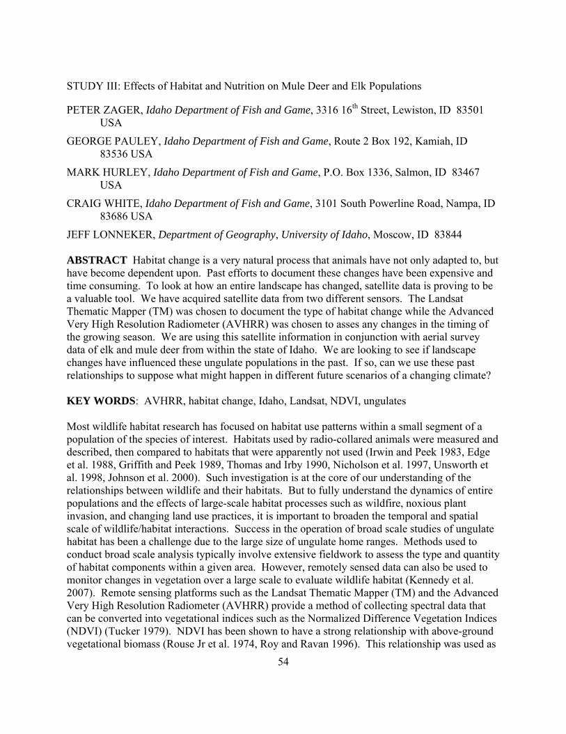
JEFF LONNEKER, Department of Geography, University of Idaho, Moscow, ID 83844 ABSTRACT Habitat change is a very natural process that animals have not only adapted to, but have become dependent upon. Past efforts to document these changes have been expensive and time consuming. To look at how an entire landscape has changed, satellite data is proving to be a valuable tool. We have acquired satellite data from two different sensors. The Landsat Thematic Mapper (TM) was chosen to document the type of habitat change while the Advanced Very High Resolution Radiometer (AVHRR) was chosen to asses any changes in the timing of the growing season. We are using this satellite information in conjunction with aerial survey data of elk and mule deer from within the state of Idaho. We are looking to see if landscape changes have influenced these ungulate populations in the past. If so, can we use these past relationships to suppose what might happen in different future scenarios of a changing climate? KEY WORDS: AVHRR, habitat change, Idaho, Landsat, NDVI, ungulates Most wildlife habitat research has focused on habitat use patterns within a small segment of a population of the species of interest. Habitats used by radio-collared animals were measured and described, then compared to habitats that were apparently not used (Irwin and Peek 1983, Edge et al. 1988, Griffith and Peek 1989, Thomas and Irby 1990, Nicholson et al. 1997, Unsworth et al. 1998, Johnson et al. 2000). Such investigation is at the core of our understanding of the relationships between wildlife and their habitats. But to fully understand the dynamics of entire populations and the effects of large-scale habitat processes such as wildfire, noxious plant invasion, and changing land use practices, it is important to broaden the temporal and spatial scale of wildlife/habitat interactions. Success in the operation of broad scale studies of ungulate habitat has been a challenge due to the large size of ungulate home ranges. Methods used to conduct broad scale analysis typically involve extensive fieldwork to assess the type and quantity of habitat components within a given area. However, remotely sensed data can also be used to monitor changes in vegetation over a large scale to evaluate wildlife habitat (Kennedy et al. 2007). Remote sensing platforms such as the Landsat Thematic Mapper (TM) and the Advanced Very High Resolution Radiometer (AVHRR) provide a method of collecting spectral data that can be converted into vegetational indices such as the Normalized Difference Vegetation Indices (NDVI) (Tucker 1979). NDVI has been shown to have a strong relationship with above-ground vegetational biomass (Rouse Jr et al. 1974, Roy and Ravan 1996). This relationship was used as

55

a proxy for vegetation in a study by Rasmussen et al. (2006) that demonstrated NDVI is a stronger predictor than seasonal rainfall of the timing of elephant calving. What this study demonstrates is the merging of remotely sensed data with ecological indicators to infer biological processes. This is a relationship that has not yet been fully explored within the ecological sciences (Hebblewhite et al. 2002). The fundamental role of remotely sensed data in the field of wildlife research has been focused on mapping species habitat and biodiversity (Laperriere et al. 1980, Huber and Casler 1990, Scott et al. 1993, Stoms and Estes 1993, Osborne et al. 2001). The Idaho Department of Fish and Game (Department) initiated this research to address the growing concern regarding ungulate habitats within the state. Fire suppression (Agee 1998), human encroachment (Unsworth et al. 1998), and noxious weed invasion (Pimentel et al. 2005) are just a few of the issues that Idaho’s wildlife face. These influences all affect the amount of forage available to ungulates. Equally as important to the amount of forage is when that forage is available to the animal (Bliss 1971). Rocky Mountain elk and mule deer are important not only in the hunting dollars that are disseminated throughout the state, but for the intrinsic value of knowing these populations are capable of continuing into the future. The impacts of habitat loss and encroachment have been shown for elk (Czech 1991, Morrison et al. 1995, Unsworth et al. 1998) but have not been as clearly defined for mule deer. Concurrently, the distribution and size of wildlife populations has also undeniably changed. Elk populations climbed to all-time highs in the 1990s but have declined in certain areas (Fig. 1). Unsworth et al (1999) noted that mule deer populations in the western United States had seen major declines in the late 1960s through the mid 1970s with a recovery about 15 years later. In the 1990s, the populations started to decline again which led to much discussion as to the possible causes and solutions (Unsworth et al. 1999). The management of wildlife populations is a complex task that forces managers to make decisions based on limited knowledge. A manager is able to influence certain aspects of population structure and size by controlling the number of hunters, season length, and hunt type, but they are not able currently to map and quantify habitat conditions (Unsworth et al. 1993). Models are helpful in informing management decisions, but one of the key factors of a model is how easily the variables are obtained. Remotely sensed data can be used to provide variables that are easily obtained, have a historical record, and can provide data in areas that might have limited field data. The information provided by this type of analysis should allow researchers and managers to monitor habitat variables on a more frequent and near real-time manner and thusly be able to make more informed management decisions.

56

Figure 1. The Idaho Department of Fish and Game has been using sightability surveys to estimate the number of elk within the state. This map depicts the estimated total elk population around 1990 when the surveys were started and the most recent surveys in roughly 2006.

57

STUDY AREAS Idaho has a wide variety of habitat types from high deserts in the southwest to dense closed canopy forests in the north. The selection of the study areas was largely driven by the availability of dependable population surveys. Elk population data has been collected systematically across the state of Idaho and provides a dataset that can be used with a relatively high degree of confidence. This made most of the Game Management Units (GMU) that contain elk available for this study. Mule deer surveys were slightly more sporadic which led to the selection of GMU 39 and the combining of GMUs 36 and 36B. Lolo Study Area The Lolo Study Area (Fig. 2) falls mainly in the Clearwater National Forest and consists of GMUs 10 and 12. It is bordered on the south by the Nez Perce National Forest, on the north by the St. Joe National Forest, on the east by the Montana border, and on the west by Dworshak Reservoir. Historically, the vegetation and habitats in this area were shaped by fire (Barrett 1982). In the early 1900s, several major wildfires swept through the area creating large shrub fields and earlier successional habitats. Such habitats were ideal for elk and the population increased to an estimated 16,119 elk in 1987. The standing vegetation is dominated by mixed mesic forest type species such as western hemlock (Tsuga heterophylla), Douglas fir (Pseudotsuga menziesii), western larch (Larix occidentalis), and western red cedar (Thuja plicata) on the north slopes, while the southern slopes are dominated by more warm mesic shrubs such as alder (alnus spp.), red-osier dogwood (Cornus sericea), mallow ninebark (Physocarpus malvaceus), chokecherry (Prunus virginiana), and woods rose (Rosa woodsii) (Landscape Dynamics Lab 1999). The area receives an average 101 cm of rain each year with nearly 60% of that falling as 267 cm of snow at Headquarters, ID (Western Regional Climate Center 2008). IDFG’s elk sightability model (Samuel et al. 1987) was developed in these GMUs giving this area the longest record of elk surveys in the state. These surveys have revealed that the elk populations in GMUs 10 and 12 have steadily declined since the early 1990s (Figures 3 and 4). Mule deer numbers for these units have been historically low and have not been surveyed. Boise River Study Area GMU 39 is the sole unit in the Boise River Study Area (Fig. 2). The eastern half of this study area falls within the Boise National Forest while the western half is dominated by the city of Boise and the surrounding agricultural and residential areas. This area has experienced massive losses of treed areas to both wildfire and insect infestation. Roughly 20% of the forest burned between 1986 and 1992. In addition, the tussock moth is credited with defoliating 225,000 acres while bark beetles killed over one half million trees during the same time period (Morelan et al. 1994). These losses have left the area dominated by warm mesic –site shrubs such as alder, oceanspray (Holodiscus discolor), western serviceberry (Amelanchier alnifolia), and devil’s club (Oplopanax horridus), while the burned areas have seen the return of early successional species. Areas in the southwestern portion consist of basin big sagebrush (Artemisia tridentata var. tridentata), four-wing saltbush (Atriplex canescens), and shadscale (Atriplex confertifolia) with

58

areas of Douglas fir (Landscape Dynamics Lab 1999). The area receives an average of 60 cm of rain each year and 207 cm of snow at Idaho City (Western Regional Climate Center 2008). While the elk populations appear to be stable or slightly increasing (Fig. 5), encroachment from development is diminishing winter range for these animals. This area represents some of the best mule deer survey data within the state of Idaho (Mike Scott, IDFG, personal communication). Radio location data has shown that most of the animals remain in this unit year round (Department, unpublished data). Challis Study Area GMUs 36 and 36B combine to make the Challis Study Area (Fig. 2). Most of this study area falls within the Challis National Forest with a portion occupied by the Sawtooth National Forest in the south. This area is vegetationally diverse with mountain big sagebrush (Artemesia tridentata var. vaseyana) and basin big sagebrush communities in the eastern portion of the study area and mixed subalpine forest, lodgepole pine (Pinus contorta), and whitebark pine (Pinus albicaulis) in the eastern and west/southwest portion (Landscape Dynamics Lab 1999). The area receives an average of 33.5 cm of rain each year and 182 cm of snow at Stanley, ID (Western Regional Climate Center 2008). Ungulates in this area typically winter in the eastern portion near agricultural areas in the lower elevations. During summer, the animals head west into the national forests. Two GMUs were combined so that any animals that were surveyed in GMU 36B during winter would have the appropriate summer habitat change measured in GMU 26. Elk populations have increased in this area (Figures 6 and 7), giving a nice contrast to the stable population in the Boise River Study Area and the declining populations in the Lolo Study Area. Mule deer population surveys have taken place in GMU 36B only, but the animals typically stay within GMU 36 during the summer months (Mark Hurley, IDFG, personal communication).

59

Figure 2. The 3 study areas were chosen to represent the differing habitat types within the state of Idaho. The Lolo study area is comprised of GMUs 10 and 12, The Boise River study area includes only GMU 39, and the Challis study area includes GMUs 36 and 36B.

60

Figure 3. Graphs depicting the relationship between different phenological metrics and calf:cow ratios in GMU 10 over time. The small numbers in the graph represent the last two digits of the year (i.e. “05” is the data point for “2005”).

100 105 110 115 120 125 130

510

1520

2530

Start of Season (Julian Day)

Cal

f/Cow

Rat

io

05

0403

0201

98

97

93

91

140 145 150

510

1520

2530

Start of Season NDVI Value

Cal

f/Cow

Rat

io

05

0403

02 01

98

97

93

91

200 210 220 230

510

1520

2530

Date of Maximum NDVI Values (Julian Day)

Cal

f/Cow

Rat

io

05

0403

0201

98

97

93

91

176 178 180 182 184

510

1520

2530

Maximum NDVI Value for Grow ing Season

Cal

f/Cow

Rat

io

05

0403

0201

98

97

93

91

220 230 240 250 260

510

1520

2530

Duration of Grow ing Season (Days)

Cal

f/Cow

Rat

io

05

0403

02 01

98

97

93

91

30 35 40

510

1520

2530

Amplitude of Grow ing Season

Cal

f/Cow

Rat

io

05

0403

0201

98

97

93

91

45 50 55 60 65 70

510

1520

2530

Time Integrated NDVI

Cal

f/Cow

Rat

io

05

0403

02 01

98

97

93

91

GMU 10 Calf:Cow Ratio vs. Phenological Metrics

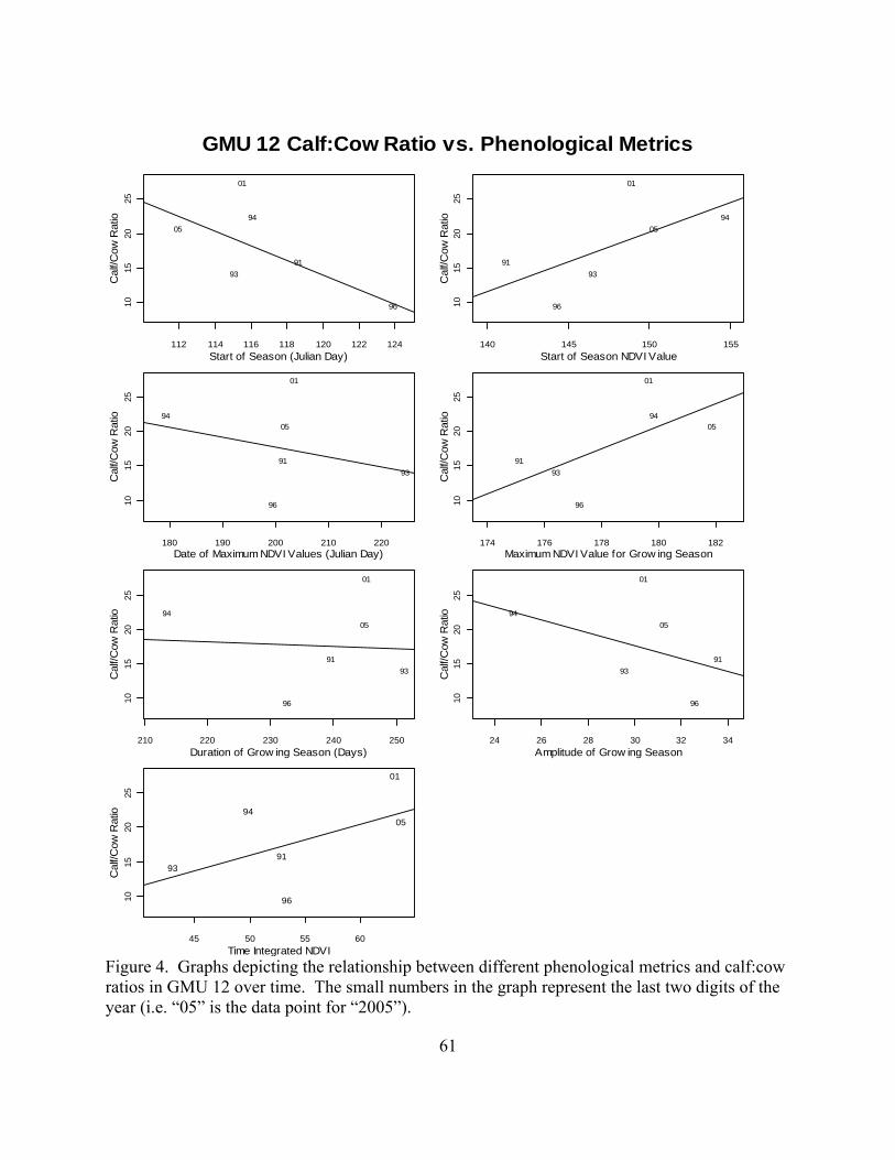
61


112 114 116 118 120 122 124

1015

2025


Cal

f/Cow

Rat

io

05

01

96

94

9391

140 145 150 155

1015

2025


Cal

f/Cow

Rat

io

05

01

96

94

9391

180 190 200 210 220

1015

2025


Cal

f/Cow

Rat

io

05

01

96

94

9391

174 176 178 180 182

1015

2025


Cal

f/Cow

Rat

io

05

01

96

94

9391

210 220 230 240 250

1015

2025


Cal

f/Cow

Rat

io

05

01

96

94

9391

24 26 28 30 32 34

1015

2025


Cal

f/Cow

Rat

io

05

01

96

94

9391

45 50 55 60

1015

2025


Cal

f/Cow

Rat

io

05

01

96

94

9391


62

Figure 5. Graphs depicting the relationship between different phenological metrics and calf:cow ratios in GMU 36 and 36B over time. The small numbers in the graph represent the last two digits of the year (i.e. “05” is the data point for “2005”).

115 120 125 130 135

1520

2530

35


Cal

f/Cow

Rat

io

04

99

96

92

129 130 131 132 133 134 135

1520

2530

35


Cal

f/Cow

Rat

io

04

99

96

92

210 215 220 225

1520

2530

35


Cal

f/Cow

Rat

io

04

99

96

92

154 156 158 160 162

1520

2530

35


Cal

f/Cow

Rat

io

04

99

96

92

220 225 230 235 240 245

1520

2530

35


Cal

f/Cow

Rat

io

04

99

96

92

20 22 24 26 28

1520

2530

35


Cal

f/Cow

Rat

io

04

99

96

92

32 34 36 38 40 42

1520

2530

35


Cal

f/Cow

Rat

io

04

99

96

92

GMU 36 and 36B Calf:Cow Ratio vs. Phenological Metrics

63


40 42 44 46 48 50 52

2530

3540

4550


Cal

f/Cow

Rat

io

04

01

99

97

95

93

91

89

126 128 130 132 134 136

2530

3540

4550


Cal

f/Cow

Rat

io

04

01

99

97

95

93

91

89

150 160 170 180 190

2530

3540

4550


Cal

f/Cow

Rat

io

04

01

99

9795

93

91

89

158 160 162 164

2530

3540

4550


Cal

f/Cow

Rat

io

04

01

99

9795

93

91

89

225 230 235 240 245 250

2530

3540

4550


Cal

f/Cow

Rat

io

04

01

99

97

95

93

91

89

22 24 26 28 30 32 34

2530

3540

4550


Cal

f/Cow

Rat

io

04

01

99

97

95

93

91

89

34 36 38 40 42 44 46

2530

3540

4550


Cal

f/Cow

Rat

io

04

01

99

97

95

93

91

89


64

METHODS The main data for this study is multispectral satellite imagery. This is imagery that goes beyond the red, green and blue that we are used to and incorporates wavelengths in the near-infrared, mid-infrared and thermal bands. This allows researchers to use the physical relationships between electromagnetic energy and vegetational structure to assess phenological processes on the surface of the planet. For instance, a healthy plant appears green because it is absorbing the red electromagnetic energy and reflecting the green. Water stored in plants cells reflects the near-infrared energy. This specific relationship is the basis for the NDVI (Tucker 1979). A high NDVI value represents healthy vegetation or a high absorption of red energy and reflection of near-infrared energy. A senesced plant will reflect the red, giving a red or brown appearance, and absorb the near-infrared energy. For this study we are focusing primarily on satellite data from two different sensors. First, the AVHRR family of sensors is a series of satellites that were first launched in October of 1978. Since then this program has been continued to provide a consistent database of multispectral data. The United States Geological Service’s (USGS) Earth Resource Observation and Science (EROS) division has worked with this data to create datasets that depict important phenological events over the course of a growing season (Table 1). These datasets are all available in raster format, with a 1 km x 1 km spatial resolution and differing temporal resolutions. With this data we are able to characterize the seasonal availability of forage. While some of our areas are in heavily coniferous forests, NDVI at large scales is still a strong predictor of forage green up (Hamel et al. 2009). With this in mind we are looking at how calf:cow ratios and doe:fawn ratios have responded to different aspects of the growing season. Pettorelli et al (2007) have used this approach to demonstrate that the rate at which forage greens up is negatively correlated with bighorn sheep lamb and mountain goat kid survival and growth rate. What this means is that if forage grows at a faster rate the adults have less exposure to high-quality forage. By using the NDVI data we will be able to see if an earlier start to a growing season is positively related to the survival success rate of calves and fawns. Initial analysis of these relationships highlights the fact that there are a limited number of data points, but it also depicts some potential relationships (Figures 3-6). We are in the process of analyzing the phenological relationships to maternal ratios and trying to understand their significance.

65

Table 1. Available data products from the USGS EROS center.

Description Acronym Brief Description Phenological Significance

Start of Season SOST Date on which the NDVI values significantly depart from the winter average.

When the first green forage becomes available.

Starting NDVI Value SOSN NDVI value on the starting day of the growing season.

The intensity with which the growing season starts.

End of Season EOST Date on which the NDVI values return to a winter average.

When vegetation senesces.

Ending NDVI Value EOSN NDVI value on the ending day of the growing season.

What was the health of the vegetation when it senesces.

Date of Maximum NDVI Value

MAXT Date on which the maximum NDVI value falls within the growing season.

Represents the length of time animals have until forage reaches maximum growth for the season.

Maximum NDVI Value

MAXN NDVI value on the date representing the maximum value for the growing season.

When the growing season peaks, how intense was it at that particular point in time.

Duration of Growing Season

DUR Length of time between the starting day and ending day of the growing season.

How long is green forage available to animals?

Amplitude of Growing Season

AMP Departure of maximum NDVI value from starting NDVI value

Gives a representation of how intense the overall growing season was


TIN Value representing accumulated biomass over entire growing season

Over the course of the growing season, this is how much overall vegetational production there was.

66

The second sensor we are using is the Landsat Thematic Mapper (TM). This family of sensors was first launched in 1972. The main difference between this sensor and the AVHRR sensor focuses mainly in the tradeoff between spatial resolution for temporal resolution. The Landsat TM has a spatial resolution of 30 m x 30 m and a return rate of every 16 days. In contrast the AVHRR sensor has a resolution of 1 km x 1 km and returns every day. We are using the Landsat TM data to generate a series of historic landcover layers and present land cover layers. These allow us to assess the type of land cover changes that have taken place in the different study areas. Each specific land cover type has a certain spectral signature almost like a fingerprint. We are able to identify this signature from known habitat types and use this to identify additional areas with the same signature. Final analysis involves elk population estimates derived from aerial sightability surveys conducted by the Department. The survey method corrects for animals that were present but not seen due to canopy closure, snow cover, and other biasing events (Samuel et al. 1987). Mule deer have not been sampled in as rigorously a method as elk. Thus, we are limited in the analysis we are able to do with the mule deer survey data. Many different factors act together to influence ungulate population dynamics such as predation (Keith 1974), interspecies competition (Carpenter 1997, Johnson et al. 2000), and habitat alteration or degradation. The latter, habitat alteration or degradation is what we focused on for this research. The seasonal availability of forage refers to when forage starts to grow, the intensity with which it grows, the duration of the growing season, and the total amount of forage produced throughout an entire season. This is important because it captures the biophenological relationship that exists between ungulates and forage. Habitat change is a natural process that animals have not only adapted to, but are dependent upon. These sensors provide are providing a unique glimpse into past phenological processes such as land cover type change and differences in growing seasons from season to season. RESULTS AND DISCUSSION Results and discussion are forthcoming in 2010 (Table 2).

67

Table 2. Graduate Student Timetable Spring 2008 Course work

Analyze status of Imagery Obtain GIS Layers

Summer 2008

Develop Proposal Develop practical methodology for spectrally and geographically correcting imagery Create Orthoreferenced Base Layers for future image correction

Fall 2008 Course work Create NDVI Dataset for Lolo Study Area Create Temporal Trajectory Dataset for Lolo Study Area Develop list of Landsat Scenes for additional study areas

Spring 2009 Course work Acquire and correct images for additional three study areas

Summer 2009

Create NDVI Datasets for remaining study areas Create Temporal Trajectory Datasets for remaining study areas. Field work: map areas of concern for temporal trajectory analysis.

Fall 2009 Course work Analyze NDVI Dataset Analyze Temporal Trajectory Dataset

Spring 2010 Finish writing thesis and journal article(s)

68

LITERATURE CITED

Agee, J. K. 1998. The landscape ecology of western forest fire regimes. Northwest Science 72:24-34.

Barrett, S. W. 1982. Fire's influence on ecosystems of the Clearwater National Forest: Cook Mountain fire history inventory. USDA Forest Service, Clearwater National Forest.

Bliss, L. C. 1971. Arctic and alpine plant life cycles. Annual Review of Ecology and Systematics 2:405-438.

Carpenter, L. H. 1997. Deer in the West. Proceedings of 1997 Deer/Elk Workshop.1 – 10.

Czech, B. 1991. Elk behavior in response to human disturbance at Mount St. Helens National Volcanic Monument.269-277.

Edge, W. D., C. L. Marcum, and S. L. Olson-Edge. 1988. Summer forage and feeding site selection by elk. Journal of Wildlife Management 52:573-577.

Griffith, B., and J. M. Peek. 1989. Mule deer use of seral stage and habitat type in bitterbrush communities. Journal of Wildlife Management 53:636-642.

Hamel, S., M. Garel, M. Festa-Bianchet, J. M. Gaillard, and S. D. Côté. 2009. Spring Normalized Difference Vegetation Index (NDVI) predicts annual variation in timing of peak faecal crude protein in mountain ungulates. Journal of Applied Ecology 46:582-589.

Hebblewhite, M., D. H. Pletscher, and P. C. Paquet. 2002. Elk population dynamics in areas with and without predation by recolonizing wolves in Banff National Park, Alberta. Canadian Journal of Zoology-Revue Canadienne De Zoologie 80:789-799.

Huber, T. P., and K. E. Casler. 1990. Initial analysis of Landsat TM data for elk habitat mapping. International Journal of Remote Sensing 11:907-912.

Irwin, L. L., and J. M. Peek. 1983. Elk habitat use relative to forest succession in Idaho. Journal of Wildlife Management 47:664-672.

Johnson, B. K., J. W. Kern, M. J. Wisdom, S. L. Findholt, and J. G. Kie. 2000. Resource selection and spatial separation of mule deer and elk during spring. Journal of Wildlife Management 64:685-697.

Keith, L. B. 1974. Some features of population dynamics in mammals. Proceedings of International Congress of Game Biologists. 2:17-58.

Kennedy, R. E., W. B. Cohen, and T. A. Schroeder. 2007. Trajectory-based change detection for automated characterization of forest disturbance dynamics. Remote Sensing of Environment 110:370-386.

69

Landscape Dynamics Lab. 1999. Land Cover of Idaho: Idaho Cooperative Fish and Wildlife Research Unit. in Moscow, Idaho, USA.

Laperriere, A. J., P. C. Lent, W. C. Gassaway, and F. A. Nodler. 1980. Use of Landsat data for moose-habitat analyses in Alaska. Journal of Wildlife Management 44:881-887.

Morelan, L. Z., S. P. Mealey, and F. O. Carroll. 1994. Forest health on the Boise National Forest. Journal of Forestry 92:22-24.

Morrison, J. R., W. J. Devergie, A. W. Alldredge, A. E. Byrne, and W. W. Andre. 1995. The effects of ski area expansion on elk. Wildlife Society Bulletin 23:481-489.

Nicholson, M. C., R. T. Bowyer, and J. G. Kie. 1997. Habitat selection and survival of mule deer: Tradeoffs associated with migration. Journal of Mammalogy 78:483-504.

Osborne, P. E., J. C. Alonso, and R. G. Bryant. 2001. Modeling landscape-scale habitat use using GIS and remote sensing: a case study with great bustards. Journal of Applied Ecology:458-471.

Pimentel, D., R. Zuniga, and D. Morrison. 2005. Update on the environmental and economic costs associated with alien-invasive species in the United States. Ecological Economics 52:273-288.

Rasmussen, H. B., G. Wittemyer, and I. Douglas-Hamilton. 2006. Predicting time-specific changes in demographic processes using remote-sensing data. Journal of Applied Ecology 43:366-376.

Rouse Jr, J. W., R. H. Haas, J. A. Schell, and D. W. Deering. 1974. Monitoring Vegetation Systems in the Great Plains with ERTS, NASA SP-351. Proceedings of Third ERTS-1 Symposium. 1:309-317.

Roy, P. S., and S. A. Ravan. 1996. Biomass estimation using satellite remote sensing data - An investigation on possible approaches for natural forest. Journal of Biosciences 21:535-561.

Samuel, M. D., E. O. Garton, M. W. Schlegel, and R. G. Carson. 1987. Visibility bias during aerial surveys of elk in northcentral Idaho. Journal of Wildlife Management 51:622-630.

Scott, J. M., F. Davis, B. Csuti, R. Noss, B. Butterfield, C. Groves, H. Anderson, S. Caicco, F. Derchia, T. C. Edwards, J. Ulliman, and R. G. Wright. 1993. GAP Analysis - A geographic approach to protection of biological diversity. Wildlife Monographs:1-41.

Stoms, D. M., and J. E. Estes. 1993. A remote-sensing research agenda for mapping and monitoring biodiversity. International Journal of Remote Sensing 14:1839-1860.

Thomas, T. R., and L. R. Irby. 1990. Habitat use and movement patterns by migrating mule deer in southeastern Idaho. Northwest Science 64:19-27.

70

Tucker, C. J. 1979. Red and photographic infrared linear combinations for monitoring vegetation. Remote Sensing of Environment 8:127-150.

Unsworth, J. W., L. Kuck, E. O. Garton, and B. R. Butterfield. 1998. Elk habitat selection on the Clearwater National Forest, Idaho. Journal of Wildlife Management 62:1255-1263.

Unsworth, J. W., L. Kuck, M. D. Scott, and E. O. Garton. 1993. Elk mortality in the Clearwater drainage of northcentral Idaho. Journal of Wildlife Management 57:495-502.

Unsworth, J. W., D. F. Pac, G. C. White, and R. M. Bartmann. 1999. Mule deer survival in Colorado, Idaho, and Montana. Journal of Wildlife Management 63:315-326.

Western Regional Climate Center. 2008. http://www.wrcc.dri.edu/index.html. in Reno, NV, USA.

71

STUDY IV: Hells Canyon Bighorn Sheep Restoration

FRANCES CASSIRER, Idaho Department of Fish and Game, 3316 16th Street, Lewiston, ID 83501 USA

ABSTRACT The Hells Canyon Initiative is a state, federal, and private partnership to restore Rocky Mountain bighorn sheep (Ovis canadensis canadensis) in the Hells Canyon area of Oregon, Idaho, and Washington. During this reporting period, 155 radio-collared bighorn sheep were monitored regularly in 12 populations. Average annual survival of radio-collared ewes was 0.88 and rams was 0.86. Lamb survival was highly variable among populations. Pneumonia-caused mortality of lambs was confirmed in 3 populations and suspected in 4 others. The overall metapopulation was estimated at 740 bighorn sheep, down from 870 bighorn sheep estimated in 2006. Multi-year collaborative projects were continued with the University of Idaho Caine Veterinary Teaching Center (CVTC) and the Department of Veterinary Microbiology and Pathology at Washington State University (WSU) to better understand the clinical causes of disease, in particular Mycoplasma ovipneumoniae, in bighorn sheep in Hells Canyon. KEY WORDS Disease, Mycoplasma ovipneumoniae Ovis canadensis canadensis Rocky Mountain bighorn sheep. The Hells Canyon Initiative was started in 1995 as a program to accelerate restoration of bighorn sheep in Hells Canyon and the surrounding areas of Idaho, Oregon, and Washington. The Initiative is to focus research applicable to bighorn sheep restoration and management throughout the western United States and Canada. The concept was formalized in 1997 with the completion of an interagency memorandum of agreement and restoration plan (Hells Canyon Bighorn Sheep Restoration Committee 1997). The restoration plan was updated in 2004 (Hells Canyon Bighorn Sheep Restoration Committee 2004). STUDY AREAS

The Hells Canyon Initiative project area encompasses 2,273,194 ha (5,617,062 ac) in the Snake River drainage in Oregon, Idaho, and Washington from the mouth of Clearwater River, Idaho, south to Brownlee Reservoir. It is bounded on the east by the hydrologic divide between the Salmon and Snake rivers near Riggins, Idaho on the Payette National Forest, Idaho, and extends just west of the Eagle Cap Wilderness, Wallowa-Whitman National Forest, Oregon. Major drainages include the Snake, Grande Ronde, Imnaha, and lower Salmon rivers. There are currently 15 bighorn sheep populations, or herds, established in the project area (Fig. 1). Over 1.3 million acres (24%) of the project area is potential bighorn sheep habitat, 68% of which is publicly owned, primarily managed by the U.S. Forest Service (USFS). Other public land managers are the states of Oregon, Idaho, and Washington and the Bureau of Land Management (BLM).

72

METHODS

Population monitoring Movements and survival of 155 radio-collared bighorn sheep (127 ewes, 43 rams) were monitored in 12 populations from 1 June 2008 to 30 May 2009. Productivity and survival of lambs born to radiocollared ewes were determined through weekly observations during lambing and lamb-rearing May – October. To estimate population size, Hells Canyon bighorn sheep were surveyed by the states of Oregon, Idaho, and Washington by helicopter (Robinson 44 and Hughes 500) and on the ground. Disease research Collaborative research continued in 2008-2009 with the Caine Veterinary Teaching Center (CVTC), and the WSU School of Veterinary Medicine to incorporate field data from Hells Canyon and elsewhere with laboratory analysis and experiments to better understand causes of pneumonia in bighorn sheep. The projects with CVTC are scheduled to continue for 1 more year and those with WSU for 2 or more years. In 2008 and 2009, projects focused on the effects and epidemiology of M. ovipneumoniae in bighorn sheep. All animal experiments were approved by the Washington State University Animal Care and Use Committee. Inoculation experiment Four M. ovipneumoniae negative captive wild-caught bighorn ewes were experimentally challenged to better understand the effect of infection with M. ovipneumoniae in bighorn sheep. Two ewes received 2 challenges 3 weeks apart in the form of antibiotic (ceftiofur)-treated M. ovipneumoniae positive lung homogenate from pneumonic lambs and two ewes received challenges on the same schedule of ceftiofur-treated nasal wash from M. ovipneumoniae-positive domestic sheep. Distribution of Mycoplasma ovipneumoniae and association with disease in bighorn sheep populations We compared culture and M. ovipneumoniae-specific polymerase chain reaction (PCR) results in healthy and diseased bighorn sheep populations from samples submitted to the Washington Animal Disease and Diagnostic Laboratory (WADDL). Contact experiment Four captive-reared bighorn sheep are being commingled with 4 domestic sheep to test the hypothesis that M. ovipneumoniae is necessary for disease transmission from domestic sheep to bighorn sheep. In the first phase of the experiment, all animals are free of M. ovipneumoniae. Previous commingling experiments between bighorn and domestic sheep have resulted in pneumonia-caused mortality of 95% of the bighorn sheep within 75 days. If the bighorn sheep

73

survive 100 days, 1 or 2 domestic sheep will be infected with M. ovipneumoniae and the experiment will be repeated with 2 of the bighorn sheep. The other 2 bighorn sheep will remain with the M. ovipneumoniae negative domestic sheep as a control. If respiratory disease or death is observed in the bighorn sheep with the M. ovipneumoniae positive domestic sheep and not in the bighorn sheep with the M. ovipneumoniae negative domestic sheep, this will be a strong case for the argument that M. ovipneumoniae is necessary for disease to occur. RESULTS AND DISCUSSION

Adult Survival

Twenty-one radio-collared adult bighorn sheep (15 ewes, 6 rams) died during this period. Cause of death could not be determined for 9 animals. Known causes of mortality were trauma (3), predation (4), pneumonia (2), hunter harvest (1), and other, noninfectious health conditions (2). Pneumonia-caused adult mortality was detected only in the Black Butte population and cougar predation was detected only in the Imnaha population. Averaged over the metapopulation, annual survival of radio-collared ewes was 0.88 and rams was 0.86. By population, annual survival of ewes in 7 populations with 6 to 15 radio-collared females ranged from a low in Imnaha of 50%, 67% at Sheep Mountain, 73% in Black Butte to 92 - 100% in the Lostine, Imnaha, Mountain View/Wenaha, Redbird, and Asotin herds (Tables 2 and 3). Lamb Survival

Lamb survival was highly variable among populations. Summer lamb survival in the 3 populations where lambs were diagnosed with pneumonia (see below) was 50% or less. Mycoplasma ovipneumoniae was detected by polymerase chain-reaction (PCR) in 7 of 9 pneumonic lambs tested (Table 4), and recruitment in these herds ranged from 5 to 22 lambs/100 ewes (Table 5). Pneumonia-caused lamb mortality was suspected in another 4 herds where summer survival was 50% or less and recruitment was 0 to 19 lambs/100 ewes (Table 4), although no dead lambs were recovered. Population Monitoring

Approximately 740 bighorn sheep are estimated to occur in 15 herds or populations within the project area (Table 6), down from the estimate of 870 in 2006-2007. Disease Research and Management

Distribution of M. ovipneumoniae in bighorn sheep populations and association with disease Besser et al. (2008) showed a strong association of M. ovipneumoniae with pneumonia in lambs in Hells Canyon, and similar association of serologic evidence of exposure to M. ovipneumoniae with disease at a population level. We observed an analogous association in samples submitted to WADDL for culture and PCR for M. ovipenumoniae. No M. ovipneumoniae was cultured from 182 bighorn sheep in populations with no evidence of disease or from bighorn sheep that died from causes other than pneumonia, although 3 samples (1.6%) were positive on PCR.

74

Twenty percent (20/100) of bighorn sheep in populations with disease-related mortality were positive on PCR for M. ovipneumoniae and 18 of 22 adult and neonate bighorn sheep (82%) that died from pneumonia were positive (Fig. 4). Challenge trial When sampled 3 weeks after the initial challenge, both groups were colonized with M. ovipneumoniae and exhibited clinical signs of respiratory disease including coughing and nasal discharge (Fig. 3). Clinical signs continued to be observed for a month and were accompanied by inappetance and lethargy. Thirty days following the second challenge, the sheep were exposed intranasally to 109 cfu of Mannheimia haemolytica causing severe pasteurellosis and death within several days to a week. Restoration Committee

The Hells Canyon Bighorn Sheep Initiative is conducted by the Hells Canyon Bighorn Sheep Restoration Committee. The committee is comprised of state, federal, tribal, and private organizations, of which each provide an administrative (A) and technical (T) committee member. Organizations and committee members in 2006 are: Idaho Department of Fish and Game

Dale E. Toweill, Wildlife Program Coordinator (A) Frances Cassirer, Tri-State Coordinator/Wildlife Research Biologist (T)

Oregon Department of Fish and Wildlife

Don Whitaker, Program Coordinator (A) Vic Coggins, District Wildlife Biologist (T)

Washington Department of Fish and Wildlife

Donny Martorello, Big Game Program Manager (A) Paul Wik, Wildlife Biologist (T)

USDA Forest Service

Bob Rock, Natural Resources Staff, Wallowa-Whitman National Forest (A) Tim Schommer, Forest Biologist, Wallowa-Whitman National Forest (T)

USDI Bureau of Land Management

Tom Rinkes, Wildlife Biologist, Idaho State Office(A) Craig Johnson, Wildlife Biologist, Salmon-Clearwater Resource Area (T)

Foundation for North American Wild Sheep

Gray Thornton, President/CEO (A) Lloyd Oldenburg and Rick Brigham, Members (T)

75

Nez Perce Tribe Loren Kronemann, Wildlife Biologist (A) Marcie Carter, Wildlife Biologist (T)

Literature Cited

Besser, T. E., E. F. Cassirer, K. A. Potter, J. VanderSchalie, A. Fischer, D. P. Knowles. D. R. Herndon, F. R. Rurangirwa, G. C. Weiser, and S. Srikumaran. 2008. Association of Mycoplasma ovipneumoniae infection with population-limiting respiratory disease in free-ranging rocky mountain bighorn sheep (Ovis canadensis canadensis). Journal of Clinical Microbiology 46: 423-430.

Hells Canyon Bighorn Sheep Restoration Committee. 1997. Restoration of Bighorn Sheep to Hells Canyon: The Hells Canyon Initiative. Technical Bulletin 97-14, Bureau of Land Management.

Hells Canyon Bighorn Sheep Restoration Committee. 2004. The Hells Canyon Initiative: Hells Canyon bighorn sheep restoration plan. Idaho Department of Fish and Game, Lewiston, USA.

76

Figure 1. Hells Canyon Initiative Project Area.

77

Figure 2. Causes of mortality of 21 adult radio-collared bighorn sheep in Hells Canyon, 1 June 2008 to 31 May 2009.

78

Figure 3. Example of clinical signs and health testing results recorded in 2008 M. ovipneumoniae challenge experiment.

Y45

0

2

4

6

8

10

12

14

5/15/2008 6/25/2008 7/5/2008 7/15/2008 7/25/2008 8/4/2008 8/14/2008 8/24/2008 9/3/2008

Date

LOG

2 Ti

ter

0

0.5

1

1.5

2

2.5

3

3.5

4

4.5

5

2 Filtr

ate ch

allen

ge

5 8 11 14 17 20 23 26 29 M

ycop

lasma c

halle

nge

32 35 38 41 44 47 50 M

ycop

lasma r

echall

enge

53 56 59 62 65 68 71 74 77 80 M

. haem

olytic

a chall

enge

Day

Scor

e

BRSV titer

PI3 titer

MOVI titer

CLINICAL SCORE

Bibersteinia trehalosi

Mannheimia haemolytica

Mycoplasma ovipneumoniae

79

Figure 4. Percent of wild sheep positive on PCR for M. ovipneumoniae in 265 samples from 5 bighorn sheep metapopulations, 2008 - 2009.

80

Table 1. Annual ewe survival in 10 Hells Canyon bighorn sheep populations, 1 June 1997 to 31 May 2009. Year Black

Butte Redbird Wenaha Asotin Lostine Imnaha Big

Canyon Muir Creek

Mountain View

Sheep Mountain

1997-1998 0.92 1 0.83 1998-1999 1 1 1 0.88 1 1 1999-2000 0.58 1 1 0.86 0.93 0.93 2000-2001 0.71 1 0.73 1 1 0.85 0.6 0.71 2001-2002 0.8 0.92 1 1 1 1 1 1 2002-2003 1 0.91 1 1 0.94 1 0.91 0.56 2003-2004 0.84 0.75 0.75 0.83 0.93 0.73 0.22 1 2004-2005 0.75 1 1 0.57 0.82 0.92 1 1 2005-2006 1 1 1 1 0.86 0.91 1 0.71 2006-2007 1 0.83 0.91 0.73 1 1 1 1 1 1

2007-2008 0.94 0.87 0.50 1 0.92 0.82 0.50 0.86

2008-2009 0.73 0.92 1 1 1 0.50 1 0.67

Average 0.86 0.93 0.89 0.90 0.94 0.86 0.85 0.88 0.83 0.84

81

Table 2. Annual ram survival in 10 Hells Canyon bighorn sheep populations, 1 June 1997 to 31 May 2009. Year Black

Butte Redbird Wenaha Asotin Lostine Imnaha Big

Canyon Muir Creek

Mountain View

Sheep Mountain

1998-1999 1 1 1999-2000 1 0.83 2000-2001 1 1 0.67 0.8 0.71 0.8 0.5 2001-2002 0.8 0.8 1 1 1 0.8 1 2002-2003 0.3 0.75 1 0.8 1 0.5 2003-2004 0.5 0.83 1 0.8 0.64 0.5 0.67 1 2004-2005 1 0.6 0.86 0.75 0.6 0.5 2005-2006 1 1 0.33 0.67 2006-2007 1 0.88 0.8 1 0.88 1 1 2007-2008 1 0.75 0.67 0.86 1 0.63 0.33 2008-2009 1 0.83 0.92 1 0.80 1 Average 0.83 0.83 0.88 0.78 0.82 0.81 0.79 0.87 0.78

82

Table 3. Observed productivity and summer lamb survival in 9 herds in Hells Canyon, 2008.

Herd No. radio-collared ewes observed with lambs (%) Percent summer survivala

Asotin Creek, Washington 8/11 (73) 88% Big Canyon, Idaho 2/2 (100) 50% (?) Black Butte, OR/WA 13/15 (87) 0 Imnaha, Oregon 11/15 (73) 27 Lostine, Oregon 10/12 (83) 20 Mtn View/Wenaha,WA OR 7/7 (100) 14 Muir Creek, Oregon 3/4 (75) 100 Redbird, Idaho 10/13 (77) 20 Sheep Mountain, Oregon 2/6 (33) 0

a Survival from birth to 1 October. Herds in bold are those where lambs were recovered with pneumonia. Table 4. Hells Canyon bighorn sheep population counts, 2008-2009.

Herd Survey date(s) Total

bighorns Ewes Lambs Rams Estimated

populationAsotin, WAa 4/5/09 83 48 18 27 90b

Bear Creek, OR 7/09 39 20 10 9 45Big Canyon, IDa 2/25/09 16 9 1 6 20Black Butte, WA/ORa 4/4/09 69 38 2 29 75Lostine, ORa 2/15/09 59 35 2 22 65Lower Hells Canyon, OR 3/14/09 36 15 5 16 40Lower Imnaha, ORa 3/17/09 114 74 14 26 135Mtn View/Wenaha, WA/ORa 3/18-19/09 89 51 11 27 120Muir Creek, ORa 2/25/09 25 11 8 6 30Myers Creek, ID 3/09 9 6 0 3 10Redbird, IDa 2/19/09 111 67 9 35 115Saddle Creek, OR 3/09 30 18 6 6 35Sheep Mountain, ORa 3/09 11 10 0 1 11Upper Hells Canyon, ID 3/09 4 2 0 2 20Upper Hells Canyon, OR 3/09 10 7 0 3 20

Total 705 741Average 49

a Populations monitored intensively under the Hells Canyon Initiative. b Eight ewes and 2 rams moved to Washington State University prior to count.

83

Table 5. Dead bighorn lambs recovered June 1, 2008 – May 31, 2009.

Hells Canyon ID # WADDL ID # Mortality Date Herd Sex Age (days, approx) Weight (kg)

Mycoplasma ovipneumoniae PCR

08WA01 2008-7838 6/20/2008 Black Butte F 30 7.7 Neg

08ID02 2008-7880 6/22/2008 Redbird M 35 10.2 Pos

08WA02 2008-7935 6/24/2008 Black Butte M 35 13.1 Pos

08WA03 2008-7999 6/25/2008 Black Butte F 35 11.6 Pos

08WA04 2008-8067 6/26/2008 Mountain View M 35 15.7 Pos 08WA05 2008-8189 6/29/2008 Black Butte M 42 .10.9 Pos

08ID03 2008-8283 7/1/2008 Redbird F 42 14 Pos

08WA06 2008-8749 7/14/2008 Black Butte M 56 13.2 No test

08WA07 2008-9242 7/23/2008 Mountain View F 56 7.5 Neg

09OR04 2009-5924 5/25/2009 Sheep Mountain M 21 7.4 Pos

84

APPENDIX 2 Progress Reports for Studies in Statewide Bird Ecology

STUDY I: Greater-Sage Grouse (Centrocercus urophasianus) lek attendance rates in southern Idaho

Greater Sage-Grouse lek attendance rates in southern Idaho

JEREMY A. BAUMGARDT, Fish and Wildlife Resources, University of Idaho, Moscow, ID 83844, USA

JOHN W. CONNELLY, Idaho Department of Fish and Game, Department of Biological Sciences, Idaho State University, Pocatello, ID 83209, USA

KERRY P. REESE, Fish and Wildlife Resources, University of Idaho, Moscow, ID 83844, USA

EDWARD O. GARTON, Fish and Wildlife Resources, University of Idaho, Moscow, ID 83844, USA

DAVID D. MUSIL, Idaho Department of Fish and Game, 319 S 417 E, Jerome, ID 83338, USA

MARC EVANS, Department of Statistics, Washington State University, Pullman, WA 99164, USA

ABSTRACT: Lek counts are used to assess population trends of Greater Sage-Grouse (Centrocercus urophasianus). Our objective is to estimate the probability of birds attending leks and the probability of detecting attending birds during a lek count in order to relate counts of birds at leks to population abundance. We also attempted to estimate survival of nests and survival of yearling and adult birds in our study population. We used mark-resighting techniques to model the probability of male greater sage-grouse attending leks and counts of grouse from blinds located within 20 m of leks to estimate detectability. Birds captured in the winters of 2006, 2007, and 2008 were fitted with 16.5 g necklace style radio transmitters. Triangulation from 2 locations off each lek was used to “re-sight” marked birds. We fit a Cormack-Jolly-Seber model to these data using Program MARK. We restricted our predictor variables to time (Julian date), year, age of birds (adult or yearling), and their interactions. The top model chosen by AIC model selection procedures included the variables of year, age, and a quadratic time trend. For our final analysis of the complete data set, we will include additional variables such as time of day and weather in our candidate set of models, which should result in more precise estimates of attendance probability. Preliminary analysis of our detectability study indicate that between 87% and 91% of the birds actually attending a lek are included in the counts preformed during a lek route. Nest success for our study area ranged from 13.3% to 27.6% during the period from 2007-2009. Further analysis of these data should produce estimates of yearling and adult survival for this population, in addition to identifying variables that affect the probability of individual birds being included in lek route counts, adult and yearling survival, and nests surviving to hatch.

KEY WORDS: Greater Sage-Grouse (Centrocercus urophasianus), lek attendance, lek route, nest survival, sightability, survival.

85

Recent trends based on population monitoring indicate that populations of Greater Sage-Grouse (Centrocercus urophasianus) are generally declining throughout their range (Connelly and Braun 1997, Connelly et al. 2004). Schroeder et al. (2004) estimated that the range of sage-grouse has shrunk to approximately 56% of the presettlement distribution. Braun (1998) stated that according to available data, the number of male sage-grouse counted on breeding grounds each spring decreased from the 1950s through the 1990s throughout their range. While these indices are somewhat crude due to the nature of historical data, they are cause for alarm and justify more intense investigation.

The mating strategy of sage-grouse offers a convenient opportunity to observe and count individuals that congregate on breeding grounds (Patterson 1952, Jenni and Hartzler 1978, Connelly et al. 2003). Each spring, males assemble and display on leks, and females visit the leks to select a male for breeding (Höglund and Alatalo 1995). Due to the conspicuousness of displaying males and the lack of cover that is typical of leks, these congregations are relatively easy to locate (Schroeder et al. 1999). Moreover, lek sites are usually traditional and persist for long periods of time (Dalke et al. 1963).

Lek routes currently provide the best index to breeding population levels throughout much of the species’ range (Connelly et al. 2000). The current method for conducting a lek route includes locating all or some portion of the leks of a breeding population visually from low-flying aircraft or audibly from the ground, identifying groups of leks for developing lek routes, then revisiting each lek within a route at least 4 times throughout the spring to count the number of males present (Connelly et al. 2003). Trends are estimated from these data by calculating the greatest number of males counted on a single visit across all leks within a route, for multiple years.

Because lek counts and lek routes may not be representative of the entire population of interest, alone they simply provide an index to breeding population levels and fall under what Anderson (2001) calls “convenience sampling”. Although these congregations of breeding sage-grouse offer easy counting of individuals, leks may not be random subsets of the population. Yearling males and adult males may not be attracted to the breeding grounds in proportion to their actual ratio, and females only spend a fraction of the time on leks that males do (Dalke et al. 1963, Jenni and Hartzler 1978, Emmons and Braun 1984, Walsh et al. 2004). Furthermore, not all birds attending a lek during a lek route census are necessarily going to be observed and included in the number reported. Size, behavior, and location within the lek may all affect the sightability of the attending birds by an observer. Any population estimates resulting from a lek route would likely be biased for a particular sex or age class, depending on the time of the counts. Moreover, using counts from a lek route to estimate numbers of male sage-grouse is of little use as no valid technique exists to assess precision of such estimates (Anderson 2001).

There are concerns with using a lek route even as an index. Using uncorrected counts as an index may be unreliable because counts are contingent upon the following assumptions: 1) the sample is proportional to the population; 2) the proportion remains constant among years when trends are estimated; 3) the proportion remains constant among sites where relative abundance is to be compared; and 4) the detection probability is the same for all observers (Anderson 2001, White 2005). Despite stringent guidelines for conducting lek routes (Connelly et al. 2003), these assumptions may not be realistic. Nichols (1992) stated that detection probabilities vary over

86

time and space due to factors that are beyond our control. Further, if these assumptions are not verified, there is a risk of reporting highly biased results (White 2005). The objectives of this project include determining: 1) how the probability of attending a lek differs among adult male, yearling male, and female sage-grouse; 2) how and what biological factors affect these probabilities; and 3) what variables affect the sightability of birds attending a lek; in order to 4) develop a method to obtain unbiased estimates of abundance for each segment of a population from lek count data. Secondary objectives of this study are to estimate survival of nests, juveniles, and adult birds, determine the sex ratio during the breeding season, and estimate the harvest rate of the study population.

STUDY AREA

Our research is being conducted on Brown’s Bench in Twin Falls County, in south central Idaho. This area extends into Elko County in north central Nevada. Brown’s Bench is bordered to the east by Salmon Falls Creek Reservoir and to the west by an area of rolling hills locally known as Monument Springs. This area receives approximately 24 cm of precipitation annually and ranges in elevation from 1524 m to 2300 m. The major cover types include low sagebrush (Artemisia arbuscula) /black sagebrush (A. nova) /grass, Wyoming sagebrush (A. tridentate ssp. wyomingensis)/grass, mountain sagebrush (A. tridentate ssp.vaseyana)/grass, mountain shrub, and crested wheatgrass seedings (Agropyron cristatum). Other, less dominant cover types include aspen woodland (Populus tremulodies), mountain mahogany woodland (Cercocarpus montanus), and wet meadow/riparian (Hironaka et al. 1983, Klott et al. 1993). Livestock grazing is the most common land use for the entire study area. The Bureau of Land Management (BLM) manages most of the land with privately owned ranches comprising the rest.

In 2007 we used 9 leks located on Brown’s Bench south of the Three Creek Road and north of the Idaho/Nevada border (Fig. 1). In 2008 and 2009, we included an additional 5 leks located north of Three Creek Road, east of Cedar Creek and west of Salmon Falls Creek. We also included an additional 2 leks within the Brown’s Bench area that were detected to be active in 2009. A preliminary study of sage-grouse in this area conducted in 2005-2006 indicated that the population was non-migratory. Nevertheless, data collected in 2007-2009 indicate that some of the birds comprising the winter population of our study area move large distances throughout the year (over 30 km) and are likely to be migratory (Connelly et al. 2000).

METHODS

Pilot Study

Trapping and marking. − In 2005-2006 male sage-grouse were captured using spotlighting (Wakkinen et al. 1992, Connelly et al. 2003) in the vicinity of the leks during early to mid-March. These males were resident in the area and had been displaying irregularly on sunny days since February. Twenty-three females (22 adults and 1 yearling) had been captured in earlier studies during previous years.

Attendance Probability and Sightability Estimation. − Lek counts by 3 observers with 1 observer counting displaying males and attending females according to the protocol by Connelly et al. (2003) commenced on 25 March and were repeated approximately weekly with the seventh

87

count occurring on 3 May 2005. Simultaneously, 2 observers located radio marked grouse using dual-element, null-peak Yagi antenna systems mounted on pickup trucks. This allowed each radio-marked grouse within radio range of the lek to be identified as to whether or not it was recorded by the first observer during the lek count.

Survival. − We will use the known-fate model in Program MARK with the following covariates to estimate survival: year, sex, age, and season. Assumptions for survival estimates from radio telemetry include: the marked sample is randomly selected from the population; marked animals are independent; marking does not influence survival; and when fate is unknown (censored) known survival time is assumed to be independent of the animal’s actual fate.

We will use Akaike’s Information Criterion (AIC) for model selection and all parameter estimates will be generated using model averaging based on AIC weights (Burnham and Anderson 1998, Murray 2006).

Field Study

Trapping and marking. − Sage-Grouse were captured using spotlighting (Wakkinen et al. 1992, Connelly et al. 2003) between late January and early March in 2007, 2008, and 2009. We attempted to capture and fit birds with radio transmitters relatively early in the winter to minimize their potential association with a particular lek as the mark-resight method we used to estimate detection probabilities relies on the assumption that samples (marked individuals) are randomly selected. We expected that random samples would help facilitate the search for new leks using radio telemetry, where selecting a sample of individuals that may have strong ties to a known lek would not likely lead to the discovery of new leks. All captured birds were classified by gender and age using wing characteristics (Dalke et al. 1963, Beck et al. 1975), and females were weighed.

In 2007, we began trapping on 18 January and continued through 15 March, at which time 32 male and 28 female sage grouse had been captured. In 2008, trapping occurred between 30 January and 15 March, during which 44 male and 17 female sage grouse were captured. In 2009, trapping began on 21 January and continued through 13 March, resulting in 47 males and 39 females captured. All captured birds were fitted with 16.5 g necklace style radio transmitters (Advanced Telemetry Systems, Isanti, Minnesota) and received a numbered aluminum leg band. In 2007, birds also received three 14 mm, colored flat-band, wrap-around style leg bands (A. C. Hughes, Middlesex, United Kingdom) in a unique combination.

Attendance Probability and Sightability Estimation. − Approximately 5 days just prior to beginning lek routes (approximately 15-20 March), we spent the early morning hours searching for previously unrecorded lek locations. We visited all suspected breeding habitat within the study area and listened for sounds of strutting males as per Connelly et al. (2003), and located radioed males. We attempted to maximize the number of leks in our routes in an effort to increase our resightings (sample size), which should improve the precision of parameter estimates (Pollock et al. 1990).

Lek routes were conducted from 20 March to 16 May in 2007, from 17 March to 21 May in 2008, and from 16 March to 27 May in 2009. Leks were counted from 0.5 hours before to 1

88

hour after sunrise when weather conditions were clear to partly cloudy and there was little to no wind (Connelly et al. 2003). In this manner, it was possible to visit 2 to 3 leks per day, allowing 15 minutes at each lek, and approximately 15 minutes to travel between leks. We included all leks in the vicinity currently included in the Idaho Department of Fish and Game (Department) standard lek route, as well as any additional ones we discovered. The number of leks in our routes ranged from 9 in 2007 to 17 in 2009. We grouped the leks in our route into twos or threes based on their proximity to each other and all leks within a group were visited on the same day. We defined a resighting occasion as the time it took for all leks within our study area to be visited exactly once and we completed a total of 8 resighting occasions in 2007, 9 in 2008, and 11 in 2009.

Lek routes were conducted by 2 researchers, each equipped with a telemetry receiver and spotting scope. Both individuals approached each lek at approximately a 90-degree arc from each other, being extremely cautious not to flush birds. Upon arriving at a predetermined position that allowed good visibility of the entire lek, the primary observer counted total number of male and female sage-grouse attending according to the protocol by Connelly et al. (2003). Both researchers then scanned through the list of frequencies of radioed birds using hand-held three-element, null-peak YAGI antenna systems, noting signals strong enough and in the general direction that would indicate positive lek attendance. We used predefined compass bearings to delineate the “edge” of the lek relative to each observation point for all leks. Items recorded included date, weather conditions, starting time, observer location, and observer’s name for each count, and number and frequency of radioed birds determined to be on the lek during a lek count. If direction and signal strength from both positions indicated the bird was likely on the lek, the bird was assumed to be attending. Researchers then moved to the next lek, repeating the previous steps.

After 2 years of pilot study, we did not feel confident with the assumption that all birds attending a lek were seen by the lek route observer, and more importantly, that radio-marked birds with signals detected on the lek were absolutely included in the count. As a result, we felt it necessary to add a detection probability or “sightability” component to our overall study.

For each day we conducted lek routes, additional personnel made observations at 1 or 2 leks from a stationary blind. We position blinds on 3 leks in 2007, on 4 in 2008, and on 6 in 2009. These leks represented the range of sizes of leks and cover types for this study area. We positioned blinds within 20 m of the edge of the leks within sagebrush to minimize potential effects the introduced structure may have on the birds’ behavior. We set up blinds no less than 1 week from the day of the first lek route to allow birds adequate time to adjust to the structure. On the day of the lek count, a single observer entered the blind 2 hours before sunrise to minimize the possibility of flushing birds. When visibility was sufficient to see birds on the lek, but no later than 0.5 hours before sunrise, each observer conducted a count of adult males, yearling males, and females visiting the lek. After each count, the observer then scanned the frequencies with a receiver and a small hand held two-element antenna for radioed birds on the lek. We recorded the following data: observer’s name, date, general weather conditions, time of each count, number of each segment of the population visually counted, number of displaying males, and number and frequency of radios heard. The observer repeated counts and frequency scans every 15 minutes. The observer continued collecting data from the blind until all of the birds left the lek.

89

Using mark-resight techniques, we used the Recaptures Only model in Program MARK to estimate the probability of attending a lek for sage-grouse from a relatively discrete breeding population. Program MARK allows the modeling of detection probabilities with group-specific, time-specific, and individual-specific covariates, which can greatly improve the precision of the estimates (White 2005). The data requirements for this model include the detection histories for each marked (radioed) bird, which is simply a record of detected or not detected for each bird during each lek route (resighting occasion). The covariates we plan to use in the model include: sex, age, date, time of day, size of lek, moon phase, weather, and year.

We used Akaike’s Information Criterion (AIC) for model selection and all parameter estimates were generated using model averaging based on AIC weights (Burnham and Anderson 1998). We used the generalized mark-resight population size estimation method described by Bowden and Kuffeld (1995) to estimate abundance and the corresponding variance for all segments of the population.

We will determine the sightability bias of sage-grouse that attend leks and use multivariate regression to evaluate effects of biologically relevant variables on the sightability of male and female sage-grouse from a lek route census. We will also develop models of visibility bias similar to those used for helicopter surveys of ungulates (Samuel et al. 1987, Bodie et al. 1995). We will use counts conducted from blinds located at the edge of leks to compare counts conducted during lek routes under the assumption that counts from the blind will include 100% of attending grouse. The variables we plan to use in the sightability model are: total number of males attending, number of yearling males attending, density and height of cover, number of females attending, time of day relative to sunrise, weather, distance to center of lek, and size (area) of lek.

Nest Survival. − For precocial species, nest survival is the probability that >1 egg hatches from a given nest, and daily nest survival rate is defined as the probability that a nest will survive a 24 hour period (Dinsmore et al. 2002). These metrics are key components of avian demographics and are used to drive and evaluate management strategies (Jehle et al. 2004, Stanley 2004).

Females with radio transmitters were located daily from the beginning of April to the end of June, or until nesting efforts ceased. We continued to monitor hens with failed nests in an effort to detect secondary nest attempts. Once hens were noted in the same location on 3 consecutive days, we attempted to get a visual confirmation of nesting without flushing the bird. Nests were then monitored daily from a single location approximately 30 m from the site to minimize disturbance (Schroeder 1997). If the female was not located on the nest, we approached the nest to determine fate. We attempted to determine fate, number of chicks hatched, or cause of failure from shell/egg remnants and other cues at the nest (Wallestad and Pyrah 1974, Martin and Guepel 1993).

We plan to use the nest survival model in Program MARK (White and Burnham 1999) to estimate daily survival and determine which biologically relevant factors affect variability of nest survival. The nest survival model in Program MARK expands on the daily nest survival model described by Bart and Robson (1982), allowing the use of individual, group-specific, and time-specific covariates (Dinsmore et al. 2002). This method does not require the restrictive

90

assumptions such as constant survival or that failure occurred at the midpoint of an interval, as do models such as Mayfield’s estimator (Jehle et al. 2004). The assumptions of this model are: (1) nests are correctly aged when first discovered; (2) nest fates are determined accurately; (3) nest monitoring does not affect survival; (4) nest fates are independent; and (5) daily nest survival rates are homogeneous.

The minimum data required for the nest survival model include: the day the nest was found; the last day the nest was checked alive; the last day the nest was checked; and the fate of the nest. We will also estimate the day incubation began from monitoring of daily hen activity so that we can include nest age as a covariate. Other covariates that will be included are: year, date of nest initiation, hen age, condition of hen at time of capture (hen weight), average temperature, and daily precipitation.

We will use Akaike’s Information Criterion (AIC) for model selection and all parameter estimates will be generated using model averaging based on AIC weights (Burnham and Anderson 1998).

Juvenile and Adult survival. − We attempted to locate all radioed birds with radio telemetry at a minimum of once per week throughout the year. UTM coordinates of each bird was recorded within 50-100 m using a hand-held GPS unit to minimize disturbance. The transmitters we used were equipped with a mortality sensor and all deceased birds were examined in the field in an attempt to determine source of mortality from the remains.

We will use the known-fate model in Program MARK with the following covariates to estimate survival: year, sex, age, and season. Assumptions for survival estimates from radio telemetry include: the marked sample is randomly selected from the population; marked animals are independent; marking does not influence survival; and when fate is unknown (censored) known survival time is assumed to be independent of the animal’s actual fate.

We will use Akaike’s Information Criterion (AIC) for model selection and all parameter estimates will be generated using model averaging based on AIC weights (Burnham and Anderson 1998, Murray 2006).

Sex Ratio. − Because hens only visit leks once or twice to choose a mate and copulate, it was not possible to detect enough radioed hens on leks to estimate their attendance probability or their population size. We will, however, be able to estimate hen population size from the estimated male population size if we can determine the sex ratio of the population.

We will estimate the sex ratio of the population of sage-grouse using 2 techniques. First, we will count males and females flushed during winter surveys. The major assumption for this technique is that field personnel can correctly recognize the sex of sage-grouse.

From areas known to be used by sage-grouse in winter, we will randomly select areas to survey from foot or vehicle. When birds flush, we will note the number of each sex and the area they flew to. Once we have sufficiently sampled an area, we will move to a new area, being careful not to re-sample the same birds during a single sampling occasion. We will repeat this procedure at least 4 times with at least a week separating each occasion.

91

Second, we will collect sage-grouse droppings from areas commonly used by sage-grouse for foraging or roosting. The droppings will then be analyzed in the lab to determine sex (Griffiths et al. 1998). The major assumptions of this method are that both male and female sage-grouse deposit droppings at the same rate, and that we can correctly identify the sex of sage-grouse from their droppings with DNA analysis. We will search areas known to be used by sage-grouse as winter forage and roost sites for freshly deposited droppings. We will search these areas by foot after a fresh snow to collect only the freshest droppings and to insure that they have been preserved (frozen) for analysis. Each dropping will be sealed in bag and labeled with the date and location it was found. Samples will then be placed in a cooler and transported to a freezer until analyzed in the lab.

Harvest. − Within the Brown’s Bench study area, there is currently a week-long hunting season each fall with a daily bag limit of 1 bird and a possession limit of 2 birds. There is strong evidence that hunting mortality is additive to winter mortality for sage-grouse (Ellison 1991, Johnson and Braun 1999, Connelly et al. 2000, Connelly et al. 2003), so understanding mortality due to harvest is crucial for proper management of the species. We used hunter returns of leg-banded birds to estimate harvest rate. Primary access to the study site is limited to a single gravel road, along which we established a hunter check station on both the opening and closing weekend of the hunting season each year. All birds reported were classified to gender and age. PRELIMINARY RESULTS

Pilot Study

Attendance Probability and Sightability Estimation. – In 2005, adult males attended leks most frequently (96%) and were counted on the leks most frequently (84% of time present within vicinity of lek; Table 1), yearling males less frequently (74% attendance and 69% detection when attending), and females rarely (15% attendance and 8% detection). Combined adult and yearling males attended during 88% of counts and were counted (observed on the lek) 79% of the time that they were present within the vicinity of a lek. Because our ultimate goal is to estimate the actual number of sage-grouse present in the entire vicinity sampled by the lek route, the most meaningful measure is the probability of detecting birds within the population. These rates are somewhat lower than attendance rates for males (68%, SE = 4.16%; Table 2) and extremely low for females (1.27%, SE = 0.90%). The same radio-marked males were seen repeatedly at leks over the course of the 7 weekly counts, but radio-marked females were only seen a single time at any lek. The maximum count for combined radio-marked and unmarked males on any of the 7 surveys was 156 birds (combined adults and yearlings). Based on the 68% (SE = 4.2%) probability of detecting radio-marked males, this outcome implies that there were a total of 233 (95% CI = 263-365) males attending the leks on Brown’s Bench during the breeding season in 2005.

Lek attendance data for 2006 have not been completely analyzed. However, it appears that peak male counts occurred much earlier in 2006 compared to 2005 (Fig. 2). In addition, the highest count of yearling males in 2006 was only 4 birds. Moreover, in 2006 yearlings had a higher probability of attending leks than adults.

92

Survival. − Survival data from 2005-2006 have not yet been analyzed.

Field Study

Attendance Probability and Sightability Estimation. − Of the 33 male sage-grouse trapped in 2007 or surviving from previous years, 5 left the study area and 5 died during or before the breeding season.

Of the 44 males captured in 2008, 29 were used for the attendance probability analysis. Of the birds censored, 3 slipped their collars, 9 died, 2 left the study area, and 1 either died or slipped its collar. Five birds surviving from 2007 with live transmitters were also included for a total sample size of 34 (30 adults and 4 yearlings).

Twenty-five of the 49 males captured in 2009 were used for the attendance analysis. Of those censored, 9 died, 8 left the study area, 1 had a faulty transmitter, and 6 either left or had faulty equipment. Thirteen birds from 2008 remained in the study, for a total sample size of 38 (36 adults and 2 yearlings).

In 2007 we conducted a total of 9 complete lek routes on the 9 leks in our study area. Additionally, we collected data from blinds on 3 of the leks for a total of 21 blind-mornings during our lek routes. We detected a total of 91 resightings of 16 adult males, 14 resightings of 3 yearling males, and a total of 8 resightings of 7 females on our study leks. The probability of detecting a marked bird on a lek in our study during the 9-week duration in 2007 was 0.63 (SD=0.23, n=17) for adult males, 0.52 (SD=0.46, n=3) for yearling males, and 0.09 (SD=0.08, n=14) for females.

In 2008 we conducted a total of 9 complete lek routes on 14 leks and collected attendance data from blinds on 4 of the leks for a total of 31 blind-mornings. We detected a total of 23 resightings of 4 yearling males and 206 resightings of 30 adult males. The probability of detecting a marked bird on our study area during the 9-week study in 2008 was 0.76 (SD=0.23, n=30) for adult males and 0.64 (SD=0.29, n=4) for yearling males.

We conducted a total of 11 complete lek routes on 17 leks and collected data from blinds on 6 distinct leks for a total of 43 blind mornings in 2009. We detected a total of 7 resightings and 271 resightings from 2 yearling and 36 adult males respectively. The probability of detecting a marked male during the 11-week study in 2009 was 0.68 (SD=0.18, n=36) for adults and 0.32 (SD=0.06, n=2) for yearlings. For the same 9-week duration used in 2007 and 2008, the detection probability in 2009 was 0.82 (SD=0.21) for adults and 0.39 (SD=0.08) for yearlings.

Peak male counts for 2008 followed a trend similar to that of 2006 and 2007 (Fig. 2) with male sage-grouse peak counts occurring relatively early in the season. Counts in 2005 followed a pattern considered normal for sage-grouse with numbers of males peaking in late April.

To date, we have modeled the 2006, 2007, and 2008 data for attendance probability. The bootstrap goodness-of-fit test in Program Mark showed our global model was a good fit to the data with only slight overdispersion (c-hat = 1.23). The top model chosen by AIC model selection procedures was an additive model with the variables of age, year, and a quadratic time

93

trend (Table 3). The next most parsimonious model resulted in Δ AIC value of 0.274 was similar to the previous model with an interaction term between year and the quadratic time trend.

A graphical representation of the predicted attendance probabilities from the models averaged based on AIC weights shows a general increase in attendance probability up to the fourth or fifth occasion (second to third week of April), followed by a decrease until the final occasion (Fig. 3). The yearling pattern of attendance appears to mimic that of the adults, but with approximately 10% lower probability of attending. An annual trend is also apparent from this Figure, with a gradual increase in attendance from 2006 through 2008. Figure 4 shows the 95% confidence limits for these estimates.

During our lek routes, we detected on average 90.88% (SD=22.99) of the total birds counted from the adjacent blind in 2007 and 87.69% (SD=24.38) in 2008.

Nest Success. − We monitored the daily movements of 17 females throughout the nesting season in 2007. We detected a total of 15 nests initiated by these hens, which included a second nest attempt from a single adult. Only 2 of the 15 nests (13.3%) successfully hatched. In 2008 we monitored 14 hens through the nesting season. We detected a total of 11 nests initiated, which again included a second nest attempt from a single adult hen. Only 3 of the 11 nests (27.3%) successfully hatched in 2008. In 2009, we detected 22 first nest attempts from 23 hens monitored. Seven of these hens also attempted a second nest, for a total of 29 nests initiated. Eight of these 29 nests produced a successful hatch, resulting in a nest success of 27.6%.

LITERATURE CITED

Anderson, D. R. 2001. The need to get the basics right in wildlife field studies. Wildlife Society Bulletin 29:1294-1297.

Bart, J. and D. S. Robson. 1982. Estimating survivorship when the subjects are visited periodically. Ecology 63:1078-1090.

Beck, T. D. I., R. B. Gill, and C. E. Braun. 1975. Sex and age determination of sage grouse from wing characteristics. Colorado Division of Game, Fish and Parks, Game Information Leaflet Number 49. Fort Collins, CO, USA

Bodie, W. L., E.O. Garton, E. R. Taylor, and M. Mccoy. 1995. A sightability model for Bighorn Sheep in Canyon Habitats. Journal of Wildlife Management 59:832-840.

Bowden, D.C., and R.C. Kufeld. 1995. Generalized mark-sight population-size estimation applied to Colorado moose. Journal of Wildlife Management 59:840-851.

Braun, C. E. 1998. Sage grouse declines in western North America: what are the problems? Proceedings of the Western Association of State Fish and Wildlife Agencies 78:139-156.

Burnham, K. P. and D. R. Anderson. 1998. Model selection and inference: a practical information-theoretic approach. New York, New York: Springer-Verlag.

94

Connelly, J. W. and C. E. Braun. 1997. Long-term changes in sage grouse (Centrocercus urophasianus) populations in western North America. Wildlife Biology 3:229-234.

Connelly, J. W., M. A. Schroeder, A. R. Sands, and C. E. Braun. 2000. Guidelines to manage sage grouse populations and their habitats. Wildlife Society Bulletin 28:967-985.

Connelly, J. W., K. P. Reese, E. O. Garton, and M. L. Commons-Kemner. 2003. Response of Greater Sage-Grouse (Centrocercus urophasianus) populations to different levels of exploitation in Idaho, USA. Wildlife Biology 9:335-340.

Connelly, J. W., S. T. Knick, M. A. Schroeder, and S. J. Stiver. 2004. Conservation Assessment of Greater Sage-Grouse and Sagebrush Habitats. Western Association of Fish and Wildlife Agencies. Unpublished Report. Cheyenne, Wyoming, USA.

Dalke, P. D., D. B. Pyrah, D. C. Stanton, J. E. Crawford, and E. F. Schlatterer. 1963. Ecology, productivity, and management of sage grouse in Idaho. Journal of Wildlife Management 27:810-841.

Dinsmore, S. J., G. C. White, and F. L. Knopf. 2002. Advanced techniques for modeling avian nest survival. Ecology 83:3476-3488.

Ellison, L. N. 1991. Shooting and compensatory mortality in Tetraonids. Ornis Scandinavica 22:229-240.

Emmons, S. R. and C. E. Braun. 1984. Lek attendance of male sage grouse. Journal of Wildlife Management 48:1023-1028.

Griffiths, R., M. C. Double, K. Orr, and R. J. G. Dawson. 1998. A DNA test to sex most birds. Molecular Ecology 7:1071-1075.

Hironaka, M., M. A. Fosberg, and A. H. Winward. 1983. Sagebrush-grass habitat types of southern Idaho. College of Forestry, Wildlife, and Range Sciences Bulletin Number 35. Moscow, ID, USA.

Hoglund, J., and R. V. Alatalo. 1995. Leks. Princeton, New Jersey: Princeton University Press.

Jehle, G., A. A. Y. Adams, J. A. Savidge, and S. K. Skagen. 2004. Nest survival estimation: a review of alternatives to the Mayfield estimator. Condor 106:472-484.

Jenni, D. A. and J. E. Hartzler. 1978. Attendance at a sage grouse lek: implications for spring censuses. Journal of Wildlife Management 42:46-52.

Johnson, K. H. and C. E. Braun. 1999. Viability and conservation of an exploited sage grouse population. Conservation Biology 13:77-84.

Klott, J. H., R. B. Smith, and C. Vullo. 1993. Sage grouse habitat use in the Brown’s Bench area of south-central Idaho. Idaho Bureau of Land Management Technical Bulletin 93-4. Boise, ID, USA.

95

Martin, T. E. and G. R. Geupel. 1993. Nest-monitoring plots - methods for locating nests and monitoring success. Journal of Field Ornithology 64:507-519.

Murray, D. L. 2006. On improving telemetry-based survival estimation. Journal of Wildlife Management 70:1530-1543.

Nichols, J. D. 1992. Capture-recapture models. Bioscience 42:94-102.

Pollock, K. H., J. D. Nichols, C. Brownie, and J. E. Hines. 1990. Statistical inference for capture-recapture experiments. Wildlife Monograph Number 107:1-97.

Patterson, R. L. 1952. The sage grouse in Wyoming. Sage Books, Denver, Colorado, USA.

Samuel, M. D., E. O. Garton, M. M. Schlegel, and R. G. Carson. 1987. Visibility bias during aerial surveys of elk in north central Idaho. Journal of Wildlife Management 51:662-630.

Schroeder, M. A. 1997. Unusually high reproductive effort by sage grouse in a fragmented habitat in north-central Washington. Condor 99:933-941.

Schroeder, M. A., J. R. Young, and C. E. Braun. 1999. Sage Grouse (Centrocercus urophasianus). In A. Poole and F. Gill [EDS.], The birds of North America, No. 425. The Birds of North America, Inc., Philadelphia, PA.

Schroeder, M. A., C. L. Aldridge, A. D. Apa, J. R. Bohne, C. E. Braun, S. D. Bunnell, J. W. Connelly, P. A. Deibert, S. C. Gardner, M. A. Hilliard, G. D. Kobriger, S. M. Mcadam, C. W. McCarthy, J. J. McCarthy, D. L. Mitchell, E. V. Rickerson, and S. J. Stiver. 2004. Distribution of Sage-Grouse in North America. Condor 106:363-376.

Stanley, T. R. 2004. Estimating stage-specific daily survival probabilities of nests when nest age is unknown. Auk 121:134-147.

Wakkinen, W. L., K. P. Reese, and J. W. Connelly. 1992. Sage grouse nest locations in relation to leks. Journal of Wildlife Management 56:381-383.

Wallestad, R. O. and D. B. Pyrah. 1974. Movement and nesting of sage grouse hens in central Montana. Journal of Wildlife Management 38:630-633.

Walsh, D. P., G. C. White, T. E. Remington, and D. C. Bowden. 2004. Evaluation of the lek-count index for Greater Sage-Grouse. Wildlife Society Bulletin 32:56-68.

White, G. C. and K. P. Burnham. 1999. Program MARK: survival estimation from populations of marked animals. Bird Study 46(Suppl):S120-139.

White, G. C. 2005. Correcting wildlife counts using detection probabilities. Wildlife Research 32:211-216.

96

Table 1. Radio-marked male and female greater sage-grouse captured and relocated in vicinity of leks on Brown’s Bench, Idaho, which were observed during 7 standard lek counts conducted from 25 March to 3 May 2005.

Demographic information Adult Males

Yearling Males Total Males Hens

Radio-tagged Individuals 12 8 20 23 Radio-weeks available during lek counts 79 47 126 157 Radio-weeks available on/near leks 76 35 111 24 No. seen during lek counts 62 24 86 2 Overall attendance rate 96.2% 74.5% 88.1% 15.3% Probability of detecting 83.8% 68.6% 78.9% 8.3% attending birds Probability of detecting 78.5% 51.1% 68.2% 1.27% birds in population (SE) (4.16%) (0.90%) Counts of all birds (w/ and w/o radios) at leks: Maximum 152 7 156 8 Mean 148.4 3.8 152.2 3.43 Projected number of birds in Population: From maximum count 233 628 From average count 196 1646

97

Table 2. Maximum number of male and female greater sage-grouse counted during 3 scans of birds present at 5 leks during 7 weekly surveys of Brown’s Bench Lek Route, Idaho, from 25 March to 3 May 2005.

Maximum Males Counted in 3 Scans

Leks 3/25 3/30 4/1 4/5 4/15 4/26 5/3 TWOSEC 1 32 52 52 47 56 34 WALTS 7 3 4 23 24 29 18 SADDLE 40 18 31 42 46 50 41 LUCUS 4 0 5 9 5 8 8

TROUGH 16 0 3 8 13 13 14 Total Males 68 53 95 134 135 156 115

Maximum Females Counted in 3 Scans

Leks 3/25 3/30 4/1 4/5 4/15 4/26 5/3 TWOSEC 0 0 0 1 0 0 0 WALTS 2 0 0 1 0 0 1 SADDLE 3 1 1 0 1 4 0 LUCUS 1 0 0 0 0 0 0

TROUGH 2 0 0 0 2 1 3 Total Females 8 1 1 2 3 5 4

Table 3. Top 7 models selected by AIC for predicting attendance probabilities of male sage-grouse on leks in 2006, 2007, and 2008.

Attendance Probability Model

AIC Delta AIC

AIC Weights

Number of Parameters

Age + Year + t2 574.872 0 0.322 6 Year * t2 + Age 575.146 0.274 0.281 10 Age * t2 + Year 577.071 2.199 0.107 8

Year + t2 577.424 2.552 0.090 5 Year * t2 577.748 2.876 0.077 9

Age * year + t2 578.921 4.049 0.043 8 Age + year + t 579.563 4.691 0.031 12

98

Figure 1. Brown’s Bench study area with leks. Asterisks indicate leks used in lek count.

99

0

5

10

15

20

25

30

35

3/22/2

007

3/29/2

007

4/5/20

07

4/12/2

007

4/19/2

007

4/26/2

007

5/3/20

07

5/10/2

007

Mla

es/le

k 200720062005

Figure 2. Lek attendance patterns on Browns Bench for 2005 through 2007.

100

Figure 3. Predicted attendance probabilities from the models averaged based on AIC weights for adult and yearling sage-grouse in 2006, 2007, and 2008.

Resighting Occasion

Atte

ndan

ce P

roba

bilit

y

0.2

0.4

0.6

0.8

1.0

2006 Adult2007 Adult2008 Adult2006 Yearling2007 Yearling2008 Yearling

18-March 1-April 15-April 29-April 13-May

101

Figure 4. Predicted attendance probabilities with 95% confidence bands from the models averaged based on AIC weights for adult and yearling sage-grouse in 2006, 2007, and 2008.

Resighting Occasion

Atte

ndan

ce P

roba

bilit

y

0.2

0.4

0.6

0.8

1.0

2006 Adult2007 Adult2008 Adult2006 Yearling2007 Yearling2008 Yearling

18-March 1-April 15-April 29-April 13-May

102


Impacts of elevated infrastructure on Greater Sage-grouse in Idaho: collision, mitigation, and spatial ecology

BRYAN S. STEVENS, Department of Fish and Wildlife Resources and Department of Statistics, University of Idaho, Moscow, ID 83844, USA.

ABSTRACT: Collision mortality is a widespread and relatively common phenomenon among European grouse. Research concerning the extent and impacts of collision mortality on North American grouse are limited. Attempts to quantify carcass retention rates associated with collision studies are available, and these usually involve monitoring collision victims or planted carcasses. However, most of these studies suggest their birds were placed “randomly”, but they either lack a strong experimental design or present extremely vague descriptions of their methods. Recent concerns involving impacts of elevated infrastructure on Greater Sage-Grouse (Centrocercus urophasianus) in Idaho have identified the lack of empirical data concerning collision frequency. The spatial extent of fences and other elevated structures has increased dramatically in sagebrush (Artemisia spp.) habitats during the last 50 years. Nevertheless, few studies have evaluated collision rates of sage-grouse over large geographic areas, and no studies have evaluated factors influencing collision rates across multiple spatial scales, further limiting our knowledge of what influences collision risk across the landscape. For these reasons, this research included the following objectives: 1) estimate collision rates of greater sage-grouse with barbed-wire fences on study areas in greater sage-grouse winter and breeding habitats, and 2) estimate carcass and collision sign detectability and longevity in sagebrush steppe habitats. During the 2009 fence surveys collision sites were located in both winter and breeding season sampling areas. In winter sampling areas 9 collision sites were located, including 1 known greater sage-grouse and 1 chukar (Alectoris chukar) collision site. However, this sampling was complicated by frequent snowfall that may have covered additional collision evidence. During lek route sampling a total of 62 avian collision sites were located, including 36 known sage-grouse, 24 unknown species and 2 western meadowlarks (Sturnella neglecta). Estimated collision rates were highly variable between seasons and study areas. In winter sampling areas collision rates for all species were 0.043 and 0.080 for individual sampling areas. Estimated fence collision rates for all species in lekking areas were highly variable, ranging from 0-2.94, and appeared to be less in subsequent sampling rounds. Global collision rate estimates treating lek routes as strata varied by sampling round from 0.062-0.493, however, not all sampling rounds contained the same number of strata. Average time to first scavenging of carcasses was similar between areas, and appeared slightly less for carcasses in big sage habitats. However, differences were observed between study sites in persistence of collision sign, although both sites showed the trend of slightly longer sign persistence in low sage habitats.

Key words: Centrocercus urophasianus, detection, Greater Sage-Grouse, fences, mortality, sagebrush

Collision mortality is a widespread and relatively common phenomenon among European grouse species (Bevanger 1990, Catt et al. 1994, Bevanger 1995b, Baines and Summers 1997, Moss et al. 2000). In Scotland, collision with deer fences is a major source of mortality for capercaillie

103

(Tetrao urogallus) (Catt et al. 1994, Baines and Summers 1997, Moss et al. 2000), and may be contributing to population declines of that species (Moss 2001). The red grouse (Lagopus lagopus scoticus) and black grouse (Tetrao tetrix) appear to be more common collision victims in Scotland than capercaillie, however, the population consequences for these species are not believed to be as severe (Baines and Summers 1997, Baines and Andrew 2003). Similarly, Norwegian studies have found collisions are a common source of mortality for capercaillie, black grouse, and ptarmigan (Lagopus spp.) in that country (Bevanger 1990, Bevanger 1995a, Bevanger 1995b, Bevanger and Brøseth 2000, Bevanger and Brøseth 2004), and collision mortality may even approach harvest mortality in some areas (Bevanger 1995b). Furthermore, grouse may be morphologically predisposed to collision mortality due to their high wing loading and heavy body weight (Janss 2000).

Research concerning the relative extent and impacts of collision mortality on North American grouse are limited. Wolfe et al. (2007) studied mortality patterns of lesser prairie-chickens (Tympanuchus pallidicinctus) in Oklahoma and New Mexico, and found 39.8% of all mortality in Oklahoma was caused by collisions with fences. Similarly, Patten et al. (2005) concluded fragmentation caused by fences, power lines, and roads in Oklahoma have resulted in higher mortality rates for female lesser prairie-chickens in Oklahoma than New Mexico. This increased female mortality has resulted in more variable nesting strategies, leading to increased vulnerability to stochastic population fluctuations (Patten et al. 2005). Additionally, Beck et al. (2006) found 33% of the juvenile mortality of Greater Sage-Grouse (Centrocercus urophasianus) on an Idaho study area was caused by collisions with power lines.

Existing research into factors influencing grouse collision mortality suggests collision may be influenced by biological, landscape, and habitat features (Bevanger 1994), however, results often vary by species or region (Baines and Summers 1997). For example, Bevanger (1995a) suggested male capercaillie and black grouse have a higher probability of collision than females due to their increased size. However, Wolfe et al. (2007) found female lesser prairie chickens were more susceptible to collision mortality due to their increased movement patterns during the breeding season. In Norway collision mortality appears to peak for ptarmigan in winter (Bevanger 1995a, Bevanger 1995b, Bevanger and Brøseth 2004) and black grouse in autumn (Bevanger 1995b), however, varied results exist for capercaillie, with studies documenting peaks in both winter (Bevanger 1995a) and spring (Bevanger 1995b). In contrast, research conducted in Scotland has shown collision mortality to peak in autumn for capercaillie (Catt et al. 1994, Baines and Summers 1997), and in spring for red and black grouse (Baines and Summers 1997), respectively. In addition to the possible influences of season and sex, research has suggested collision mortality in grouse may be influenced by the structure, type, and height of surrounding vegetation (Bevanger 1990, Catt et al. 1994, Baines and Summers 1997, Bevanger and Brøseth 2004), topography (Bevanger 1990), and local bird densities (Baines and Andrew 2003, Bevanger and Brøseth 2004). Furthermore, some authors have found evidence for collision “hot spots” where mortality is concentrated (Bevanger and Brøseth 2000, Baines and Andrew 2003), while others have not found evidence for clumped collision distributions (Baines and Summers 1997).

In a review of the interactions of birds with utility infrastructure, Bevanger (1994) suggested that factors influencing collision can be classified as biological, topographical, meteorological, or technical. Biological factors influencing collision risk include the previously mentioned high

104

wing loading and heavy body weight (Bevanger 1998, Janss 2000), as well as factors such as vision (Bevanger 1994), crepuscular or nocturnal activity patterns (Avery et al. 1978), and local or migratory movement patterns (Avery et al. 1978, Meyer 1978, Malcom 1982). Several studies have suggested that collision rate is influenced by the number of birds using a particular area (Baines and Andrew 2003, Bevanger and Brøseth 2004), while other studies have found no relationships between the number of collision mortalities and local bird densities (Rusz et al. 1986, Cooper and Day 1998). Structural features of vegetation that have influenced collision risk include the vegetation type (Bevanger 1990, Baines and Summers 1997), the distance between the structure and surrounding vegetation (Bevanger 1990, Catt et al. 1994), and the relationship between the structure height and vegetation height (Bevanger 1990, Catt et al. 1994, Bevanger and Brøseth 2004). Topographical features influencing collision rates include mountain valleys and coastlines (Cooper and Day 1998), as well as sloping terrain and ridges (Bevanger 1990), and other features that influence local or migratory movement corridors (Bevanger 1994).

In addition to the influence of biological and topographical features on collision, risk may also be influenced by meteorological conditions and infrastructure design (Bevanger 1994). Meteorological conditions influencing collision risk include fog, precipitation, strong winds, and other weather conditions influencing bird flight intensity and behavior (Bevanger 1994). Although there is ample evidence for changes in flight behavior due to weather conditions (Meyer 1978, James and Haak 1978, Brown and Drewien 1995, Savereno et al. 1996), evidence for increased collision risk due to weather conditions is mostly anecdotal, as many studies have inconclusive empirical results concerning collision rates and weather variables (Meyer 1978, James and Haak 1978, Beaulaurier 1981, Savereno et al. 1996). In contrast, Brown and Drewien (1995) found increased collision rates during periods of strong gusty winds; however, they found no relationship between collision rates and precipitation. Technical designs related to infrastructure construction may also influence collision risk (Bevanger 1994). However, Janss (2000) suggested there is not strong empirical evidence that infrastructure design influences risk, a conclusion shared by other authors (Bevanger and Brøseth 2000, Bevanger and Brøseth 2004). One exception to the lack of empirical evidence concerning the impact of infrastructure design on collision risk is the presence of overhead ground wires on power lines, which often increase collision mortality rates (Myer 1978, James and Haak 1978, Beaulaurier 1981).

There are 2 common approaches to estimating collision rates of birds with elevated infrastructure. The first approach involves placing observers in ground blinds to physically watch power line or fence sections for collisions during daylight hours (Meyer 1978, James and Haak 1979, Beaulaurier 1981, Brown and Drewien 1995). While this method may be appropriate for known problem areas containing large numbers of birds, this method is inefficient and ineffective for estimating collision rates over larger geographic areas (Bevanger 1999). A second method commonly used involves searchers walking along power line corridors or fence sections to locate collision victims (Meyer 1978, James and Haak 1979, Bevanger et al. 1994, Baines and Summers 1997, Baines and Andrew 2003, Bevanger and Brøseth 2004). While this method is more effective for determining collision rates over large areas, there are several potential biasing factors in collision estimates associated with searching for carcasses in this manner.

105

Two major biasing factors associated with estimating collision rates through ground searches include detectability and scavenging bias (Bevanger 1999). Detectability bias is common in many studies, and can be influenced by factors such as meteorological conditions, snow cover, size of the bird under study, local vegetation, and the ability of the field workers (Bevanger 1999). Scavenging bias refers to a collision victim being removed by scavenging animals prior to detection by observers (Bevanger 1999, Smallwood 2007).

Numerous attempts to quantify carcass retention rates associated with collision studies are available, and these usually involve monitoring collision victims (James and Haak 1979) or planted carcasses (Lee 1978, Meyer 1978, James and Haak 1979, Beaulaurier 1981). Most of the previous studies regarding carcass retention suggest their birds were placed “randomly”, however, they either lack a strong experimental design or present extremely vague descriptions of their methods (Pain 1991, Baines and Summers 1997, Bevanger and Brøseth 2004). For example, Pain (1991) placed both male and female mallards in differing habitats to assess the influence of cover and sex on scavenging rates, but failed to adequately describe the experimental design used. Similarly, Baines and Summers (1997) mentioned in their results that 18 of 20 red grouse (Lagopus lagopus scoticus) placed near fences were gone after 1 month, however they did not provide an adequate description of the experimental design used in their methods. The accuracy and applicability of scavenging rates calculated in many studies are also hindered by extremely small sample sizes (Meyer 1978, James and Haak 1979, Beaulaurier 1981, Savereno et al. 1996).

In addition to small sample sizes and vague descriptions of methodology, Smallwood (2007) suggested that much of the previous research has fundamentally asked the wrong questions, testing for differences only between areas (Meyer 1978, Beaulaurier 1981, Bevanger and Brøseth 2000) without addressing other factors that could influence scavenging rates. For example, Bevanger and Brøseth (2004) tested for differences in scavenger removal rates between fence sections, without considering the influence of any other factors. Additionally, Bevanger et al. (1994) developed a model to incorporate scavenging rates into collision estimates by calculating the probability that a bird killed during the interval between searches was still present, however, the probability depended only on the length of time between patrols without considering any other factors that could have influenced scavenging rates, such as habitat type or season of year.

Although the majority of studies incorporating carcass retention estimates only considered scavenging rates as a function of time, several studies evaluated the influence of other factors. Linz et al. (1991) evaluated the influence of carcass density and water depth on scavenging rates of red-winged blackbirds (Agelaius phoeniceus) in cattail marshes. In this study scavenging rates were increased in plots with high carcass densities, and lower in deeper water than shallow water (Linz et al. 1991). Additionally, Bumann and Stauffer (2002) examined the influence of carcass condition, stand type, overhead cover, temperature, and habitat variables on scavenging rates of ruffed grouse (Bonasa umbellus) in Appalachia. While scavenging was not influenced by any habitat variables, the probability of scavenging was higher for mock avian killed birds than whole carcasses, and higher with increasing air temperatures (Bumann and Stauffer 2002). The authors believed that birds with exposed viscera likely provided stronger olfactory stimulus to scavengers in this study (Bumann and Stauffer 2002). In contrast, studies using songbird carcasses have found differences in carcass retention between different habitat types (Linz et al. 1997, Kostecke et al. 2001). Furthermore, Smallwood (2007) found evidence for seasonal

106

variation in scavenging rates of birds killed by windmills, with the highest scavenging rates occurring in the fall. Finally, common metrics used to summarize scavenging rates such as mean time to removal can be severely biased by the length of the removal trials and the sample size of carcasses used; often leading to unreliable mortality estimates (Smallwood 2007).

Much like estimates of carcass retention, estimates of carcass detectability commonly accompany avian collision mortality studies (Anderson 1978, Meyer 1978, James and Haak 1979, Beaulaurier 1981, Bevanger 1999). Although most of these studies have calculated detectability rates on their study areas to correct mortality estimates, many have failed to quantify the factors influencing detectability (i.e. Anderson 1978, Meyer 1978, James and Haak 1978, Beaulaurier 1981, Bevanger 1995, Brown and Drewien 1995, Savereno et al. 1996). Carcass detectability is likely influenced by the species of interest, local terrain, vegetation, searcher experience, and meteorological conditions (Beaulaurier 1981, Bevanger 1999), however, these sources of variability are rarely addressed (Smallwood 2007). Linz et al. (1991) evaluated the influence of carcass density and sex of red-winged blackbirds in cattail marshes on carcass detectability, and found higher detectability for male (83%) than female (78%) blackbirds. Similarly, Osborn et al. (2000) evaluated the influence of season, vegetation height, and snow cover on detectability of birds on wind farms in Minnesota. In this study detectability was only influenced by the size of the bird, with large birds having a higher detection rate (92.3%) than small birds (68.7%) (Osborn et al. 2000). Additionally, Smallwood (2007) examined the influence of vegetation height and bird group on detectability of windmill collision victims. This study found detectability varied by the bird group under study (i.e. large raptors, large non-raptors, etc.), while vegetation height only influenced detection for small non-raptor birds (Smallwood 2007).

Recent concerns involving impacts of elevated infrastructure on greater sage-grouse in Idaho (Idaho Sage-Grouse Advisory Committee 2006) have identified the lack of empirical data concerning collision frequency and grouse in North America. The spatial extent of fences and other elevated structures has increased dramatically in sagebrush habitats during the last 50 years (Connelly et al. 2000, Connelly et al. 2004), and their potential impact on sage-grouse has not gone unnoticed (Braun 1998, Connelly et al. 2000, Connelly et al. 2004). Previous studies involving collision mortality have often focused on presumed collision “hot spots” (Meyer 1978, James and Haak 1978, Beaulaurier 1981, Brown and Drewien 1995, Savereno et al. 1996), however, these presumptions were never verified. These methods have provided intensive studies over spatially small sites with limited application to other areas. Baines and Summers (1997) evaluated grouse collision mortality over a large geographic area in Scotland, but only considered the influence of factors at the collision site scale. Thus, few studies have evaluated collision rates over large geographic areas, and no studies have evaluated factors influencing collision rates across multiple spatial scales, further limiting our knowledge of what influences collision risk across the landscape. For these reasons, this research was pursued with the following objectives: 1) estimate collision rates of greater sage-grouse with barbed-wire fences on study areas in Greater sage-grouse winter and breeding habitats, 2) estimate carcass and collision sign detectability and longevity in sagebrush steppe habitats.

107

STUDY AREA

Fence Sampling and Collision Estimation

Fence sampling for collision rate estimation in potential greater sage-grouse winter habitat was conducted on 2 study areas, 1 each in the Magic Valley and Upper Snake regions. Winter fence sampling in the Magic Valley region was conducted on an area I am referring to as the East Jarbidge (EJ) sampling area, consisting of the Antelope Pocket and Browns Bench geographic regions. This study area was bound to the north by the confluence of the Salmon Falls Creek and Cedar Creek canyons, and to the south by the Nevada state line. The western boundary of the EJ sampling area was formed by the Cedar Creek canyon north of Three Creek Road and the Monument Springs hills south of Three Creek Road, while the eastern boundary was approximately the Salmon Falls Creek canyon north of Three Creek Road and Salmon Falls Creek reservoir south of Three Creek Road, respectively. Elevations on this sampling area ranged from approximately 1450-1775 m, and habitat conditions were dominated by low sagebrush (Artemisia arbuscula) in the southern portion of the study area (south of Three Creek Road), and big sagebrush (Artemisia tridentata) in the northern areas (north of Three Creek Road). However, habitat conditions in sampled areas were variable and ranged from dense stands of sagebrush to bare pasture and large stands of crested wheatgrass (Agropyron cristatum). Additionally, riparian areas south of Three Creek Road commonly contained stands of big sagebrush.

Winter sampling in the Upper Snake region was conducted on an area referred to as the Upper Snake (US) sampling area, consisting primarily of the Table Butte and Lidy Flats geographic regions. The Table Butte portion of the study area was bound to the east by U.S. highway 15 and to the north, south, and west by the BLM property boundary in that area. The Lidy Flats portion of the US sampling area was bound approximately by U.S. 15 to the East, Idaho state route 22 to the south, and the Medicine Lodge hills to the north and west. Elevations in the US sampling area were similar to the EJ sampling area, and habitat conditions varied from large stands of low sagebrush in the Lidy Flats area to stands of big sagebrush and large grasslands in the Table Butte area. However, the US sampling areas were primarily covered in snow ranging from approximately 0.25-0.75 m deep during the winter sampling period.

Fence collision surveys in Greater sage-grouse lekking areas occurred in 16 Department monitored lek routes across 4 large geographic regions of southern Idaho. In the East Jarbidge region previously described fence was sampled in 2 lek routes, the Antelope Pocket and Browns Bench routes, respectively. In the northern Magic Valley region, fence was sampled in 4 lek routes, the North Shoshone, Timmerman, Picabo Hills, and Paddleford Flats routes. In the Big Desert region south of Arco, fence was sampled in 4 lek routes, the Big Desert routes 1, 3, and 5, as well as the Fingers Butte route. Finally, in the Upper Snake region of southeast Idaho, fence was sampled in 6 lek routes, the Crooked Creek, Lidy, Table Butte, Medicine Lodge, Plano, and Red Road routes. Elevations on breeding season sampling areas ranged from approximately 1450 m on the Browns Bench lek route to approximately 2000 m on the northern portions of the Red Road and Medicine Lodge lek routes. Habitat types on the breeding season sampling areas once again varied considerably, from large stands of big, low or mixed sagebrush types, to large

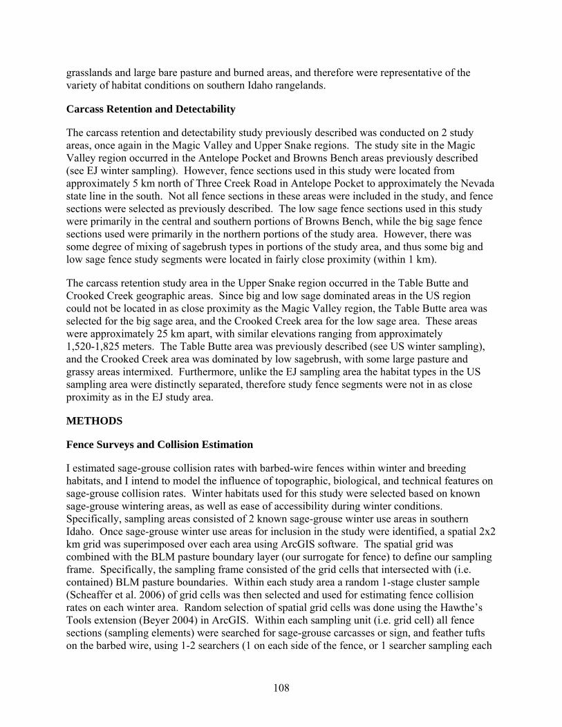
108

grasslands and large bare pasture and burned areas, and therefore were representative of the variety of habitat conditions on southern Idaho rangelands.

Carcass Retention and Detectability

The carcass retention and detectability study previously described was conducted on 2 study areas, once again in the Magic Valley and Upper Snake regions. The study site in the Magic Valley region occurred in the Antelope Pocket and Browns Bench areas previously described (see EJ winter sampling). However, fence sections used in this study were located from approximately 5 km north of Three Creek Road in Antelope Pocket to approximately the Nevada state line in the south. Not all fence sections in these areas were included in the study, and fence sections were selected as previously described. The low sage fence sections used in this study were primarily in the central and southern portions of Browns Bench, while the big sage fence sections used were primarily in the northern portions of the study area. However, there was some degree of mixing of sagebrush types in portions of the study area, and thus some big and low sage fence study segments were located in fairly close proximity (within 1 km).

The carcass retention study area in the Upper Snake region occurred in the Table Butte and Crooked Creek geographic areas. Since big and low sage dominated areas in the US region could not be located in as close proximity as the Magic Valley region, the Table Butte area was selected for the big sage area, and the Crooked Creek area for the low sage area. These areas were approximately 25 km apart, with similar elevations ranging from approximately 1,520-1,825 meters. The Table Butte area was previously described (see US winter sampling), and the Crooked Creek area was dominated by low sagebrush, with some large pasture and grassy areas intermixed. Furthermore, unlike the EJ sampling area the habitat types in the US sampling area were distinctly separated, therefore study fence segments were not in as close proximity as in the EJ study area.

METHODS

Fence Surveys and Collision Estimation

I estimated sage-grouse collision rates with barbed-wire fences within winter and breeding habitats, and I intend to model the influence of topographic, biological, and technical features on sage-grouse collision rates. Winter habitats used for this study were selected based on known sage-grouse wintering areas, as well as ease of accessibility during winter conditions. Specifically, sampling areas consisted of 2 known sage-grouse winter use areas in southern Idaho. Once sage-grouse winter use areas for inclusion in the study were identified, a spatial 2x2 km grid was superimposed over each area using ArcGIS software. The spatial grid was combined with the BLM pasture boundary layer (our surrogate for fence) to define our sampling frame. Specifically, the sampling frame consisted of the grid cells that intersected with (i.e. contained) BLM pasture boundaries. Within each study area a random 1-stage cluster sample (Scheaffer et al. 2006) of grid cells was then selected and used for estimating fence collision rates on each winter area. Random selection of spatial grid cells was done using the Hawthe’s Tools extension (Beyer 2004) in ArcGIS. Within each sampling unit (i.e. grid cell) all fence sections (sampling elements) were searched for sage-grouse carcasses or sign, and feather tufts on the barbed wire, using 1-2 searchers (1 on each side of the fence, or 1 searcher sampling each

109

side in turn). Previously unidentified fence segments (i.e. not identified with the BLM pasture boundary layer), as well as all fence types inside our spatial clusters were digitized using handheld GPS units and ArcGIS software. Sampling of fence sections occurred from 22 January – 25 February 2009 on sage-grouse winter use areas. During these surveys fence searchers walked approximately 1-3 m on either side of the fence, and monitored the area up to approximately 15 m from each side of the fence for carcasses or collision evidence.

Statistical estimation of the average number of collisions per linear kilometer of fence (i.e. collision rate) and total number of collisions located on each study area in winter habitat follows from elementary sampling theory (i.e. Scheaffer et al. 2006). Specifically, estimation of the collision rates ( ) and variance of the rates ( ( )) on each study area were calculated as follows:

Where:

Notation in these formulas represents the following values: the total number of clusters in the population; = the number of clusters sampled; = the length of fence in kilometers in cluster ; = the average length of fence in kilometers per cluster in the sample; and = the number of collision sites located in the cluster. It should also be noted that in the variance formula is used instead of the true average cluster size for the population ( ) which is unknown. Furthermore, estimation of the total number of collision sites on each study area ( ) and variance of this estimate ( ( )) were calculated as follows:

Where:

110

It is important to note that (the average number of collision sites located in the clusters sampled) is not the same as (the average number of collision sites located per linear kilometer of fence) as calculated in equation one.

A collision in this study was defined as detection of a whole carcass or a feather pile (>5 feathers) within 15 m of the fence, or detection of feather tufts stuck in the barbed-wire fence. Despite this definition of a collision we were cautious when only feather sign was detected, and if a likely avian plucking post was present we were conservative and did not call these sites collision locations. For example, plucking posts were common in some areas (mostly for passerine species) and were usually located at large wooden fence-posts, with the resulting feather piles scattered from the base of the post in the prevailing wind direction. In contrast, sites deemed collision locations based solely on feather-pile evidence commonly contained large numbers of feathers scattered in the prevailing wind direction from under the fence itself, or very close to the fence. Given this definition of a fence collision the only victims not accounted for would involve birds flying into fences and leaving no feathers either in the fence or on the ground, and no carcass. During our searches feather tufts and piles were counted as collisions with no knowledge of the fate of the collision victim. Therefore our estimates are of the number of collision sites present at the time of the survey, and not of collision mortalities, as we had no way to assess the crippling bias caused by individual birds flying into fences and dying at a later time or in a different area (Bevanger 1999). Furthermore, this estimate is likely biased low due to an unknown detection probability for collision evidence in sagebrush-steppe habitats. The assumption that collision brings no benefit and is always associated with negative effects on the individual victims is inherent in this methodology. Thus, the relationship between the collision itself and the extent of the negative effects on the individual birds was left unstudied, as this is extremely difficult to accurately assess (Bevanger 1999).

To assess the significance of features recorded at collision locations, random points were selected on each study area for site scale analysis of factors influencing collision. Specifically, 1 spatial location for each collision victim found on each study area was randomly generated within the sampling frame using the Hawthe’s Tools extension (Beyer 2004) of ArcGIS software, and the closest fence segment to this location on the study area was used to measure site-scale variables that will be used in modeling.

A cluster sampling approach was also used to estimate collision rates in sage-grouse breeding habitat. The methods used were modified slightly from the surveys of sage-grouse winter habitat to encompass a larger geographic extent. Specifically, 16 lek routes monitored by the Department were selected for inclusion in the study based on accessibility and known breeding bird use. Once lek routes were selected, global collision rates were estimated using stratified cluster-sampling framework (Scheaffer et al. 2006). Specifically, once the 16 lek routes (strata) were selected each lek in the route with ≥1 displaying male documented the previous year (2008) was buffered by 1.5 km using ArcGIS software. Once each lek route was buffered, a 1x1 km spatial grid was superimposed over the buffered leks within each route using ArcGIS software, and the grid cells that intersected with (i.e. contained) BLM pasture boundaries (our surrogate for fence) were used to define the sampling frame. Once the sampling frame was defined for each lek route a stratified cluster sample of 1x1 km grid cells was randomly selected using the Hawthe’s Tools (Beyer 2004) extension in ArcGIS. I allocated the sample of 60 grid cells to each stratum in proportion to the number of cells in each stratum. For example, if 1 strata (lek

111

route) contained 10% of the total number of cells in the sampling frame, then that strata was allocated 6 sample cells (10% of 60). Sixty cells was selected as the overall sample size because I estimated this as the maximum number of cells that could be sampled in a one month period given time and logistical constraints, which was needed to facilitate repeat sampling necessary to incorporate temporal variability in lek dynamics.

Within randomly selected cells, all fence sections (sampling elements) were searched for fence collision victims, and new fence segments digitized as previously described. The radius of 1.5 km that was used to buffer leks was selected in attempt to maximize the areas sampled in breeding habitats, while simultaneously minimizing the time spent sampling each area. Minimizing time spent at each location was needed to facilitate repeat visits to sites. Furthermore, 1x1 km sampling grids did not line up perfectly with the lek buffer boundaries, making approximately 2.5 km the maximum possible distance of a sampled fence segment from the given lek. Finally, fence sampling occurred from 5 March – 19 May 2009 on sage-grouse breeding areas.

Statistical estimation of collision rates and total numbers of collision sites in the breeding areas once again followed from elementary sampling theory (Scheaffer et al. 2006). Estimates of the collision rates ( ) and variance of the rates ( ( )), as well as the total number of collision sites ( ) and variance of this estimate ( ( )) within each strata were calculated using equations 1-6 similar to a 1-stage cluster sample. A global estimate of collision rates over all strata is analogous to a combined form ratio estimate, consisting of the ratio of the estimated average cluster total (i.e. average number of collisions detected per cluster) to an estimator of the average cluster size (i.e. average length of fence in kilometers per cluster). Estimates of the population average per linear kilometer of fence (i.e. population average collision rate) ( ) and its variance ( are as follows:

Where:

Notation used in these formulas represents the following values: N = total number of clusters in the strata; = total number of clusters in the th strata; = the number of clusters sampled in the th strata; = the number of collisions detected in the th cluster of the th strata;

112

= the length of fence in kilometers in the th cluster of the th strata; = average number of collision sites located in clusters of the th strata (total number of collisions located / total number of clusters sampled); and = average length of fence in kilometers of clusters in the th strata (total length of fence / total number of clusters sampled). In the above equation for

the term was used because the total length of fence in the population of clusters ( ) was unknown.

The methods used will limit the inference of our estimates on breeding areas to fence collision rates within approximately 2.5 km of leks within a given region; however, this allowed sampling a larger geographic extent across southern Idaho. Since the extent of collision risk across the landscape for sage-grouse has never been investigated, I felt it was important to cover a broad geographic extent although this will limit the intensity with which we can sample in any given region. Similar to the winter use areas, random locations were selected for comparison of collision site scale variables. Specifically, these random points were selected from all available locations within sampling frame of each sampled lek route, and variables were recorded at the closest fence segment to this point.

Once collision evidence was located during fence searches, biological, topographical and technical characteristics of the collision site were recorded. If collision sign was located without evidence present on the fence, all collision site measurements were made at the fence location perpendicular to the closest collision evidence. For example, feather pile evidence was often scattered by the wind from a location under or very close to fence, and the closest evidence (i.e. feather or group of feathers) was used to determine the point used for measurements. Biological variables collected at each collision site include the species, sex, age of the victim (if possible), the type of evidence found, and the perpendicular distance to the closest, farthest, and first detected collision evidence located, as well as the vegetation characteristics at the collision site. Initially we attempted to determine direction of flight; however, this appeared unreliable and therefore was no longer attempted. Vegetation height of the closest shrub from each side of the fence not intersecting the plane of the fence, distance to the closest non-intersecting shrub on each side of the fence, and canopy coverage along 10 m transects (Canfield 1941) in the cardinal directions centered on the collision location were collected. Height of the closest shrub growing directly along the fence (i.e. intersecting the plane of the fence) within 5 m of the collision site in both directions was measured to evaluate the influence of vegetation in the longitudinal direction of the fence. Technical variables collected at each collision site include fence height, fence type, and the distance between fence posts. Finally, topographic variables collected included UTM location, and slope both across and along the fence (measured over 20 m centered on the collision site). Additionally, aspect at each collision site and random sites will be obtained using a digital elevation model in ArcGIS. The lek count (provided by IDFG), and difference between vegetation height and the fence height will be calculated to include in modeling. Furthermore, the distance of the collision site to the nearest known lek will be recorded at a later date using ArcGIS software. Additionally, all previously mentioned data not involving leks, as well as snow depths at 1 m perpendicular to the fence on both sides was collected at collision locations and random points in winter habitat.

113


This study used pen-raised hen ring-necked pheasant (Phasianus colchicus) carcasses as the sampling unit to evaluate factors influencing scavenging and detectability of fence collision victims in sagebrush-steppe habitats. This was done using a completely randomized design (Ott and Longnecker 2001) with 2 levels of treatment effects for habitat type (big sage or low sage), and carcass distance from the fence as a covariate, with carcasses placed at random distances from 0-15 meters. Additionally, feathers were removed from the front of the breast of each bird, and 10-15 feathers were placed immediately around each carcass. Feather piles of 10-15 breast feathers were placed similarly to carcasses to determine feather detectability, as it could differ from that of carcasses. Therefore, the influence of the previously mentioned factors on the detectability and longevity was measured for collision sign (i.e. feathers piles) in addition to the carcasses. Placing feathers around each carcass prevented a carcass from being removed and leaving no visible sign, a scenario that is unlikely with collision victims as feathers will likely fall when birds strike fences. Detection of a collision will be defined as detection of a carcass, feather tufts in the fence, or feather piles near the fence (>5 feathers within 15 m). This allowed quantification of the factors influencing detectability and longevity for all sources of a detected collision, with the exception of feathers lodged in the barbed-wire fence. Furthermore, this design was replicated on both the East Jarbidge and Upper Snake study areas, to allow detection of regional differences in carcass longevity. Detectability was only measured on the East Jarbidge study area due to a lack of field volunteers to sample fences on the Upper Snake study area.

Available fences in each habitat type on each study area were quantified using ground searches, handheld GPS units, and ArcGIS software. The fence sections located in each habitat type were mapped out by taking GPS waypoints along and at the ends of each fence section, then digitizing the fence segments in ArcGIS. Because sagebrush-steppe habitats often have a patchy mosaic of sagebrush, pasture, and grassy areas, only fence segments that were traversing areas dominated on both sides by the desired habitat type were included in this study. Once fence sections were digitized the ArcGIS extension Hawthe’s Tools (Beyer 2004) was used to generate random fence points >200 m apart in each habitat type. Fifty bird carcasses were placed on each study area, 25 replicates for each treatment level. In addition to the 50 points generated on each area for placement of pheasant carcasses, 50 points (25 for each treatment) were generated in a similar manner on the East Jarbidge study area for placement of feather piles used in detectability trials. Furthermore, prior to field placement all randomly generated points were ground verified to be in the desired habitat type, and those points not in the desired habitat (i.e. where desired habitat did not dominate both sides of the fence) were discarded. Additionally, no fence sections running along paved roads were used in this study, as this could bias results if predators used or avoided these roads. Fence sections running along unimproved or gravel roads were included in this study due to the abundance of unimproved roads and 2-tracks on the study areas. Road presence will be treated as a random covariate to incorporate variability in scavenging due to fence sections running along unimproved roads. Finally, the side of the fence used for carcass placement was randomly selected for fences entirely on public land. For fence segments bordering private land only the public side was used for pheasant placement and detectability searches.

114

Bumann and Stauffer (2002) placed ruffed grouse carcasses >100 m apart in their Appalachian study, however, sagebrush-steppe habitats are more open than deciduous forest, and larger inter-carcass distances are likely necessary. Therefore, my methods ensured that carcass locations were no closer than 200 m on any portion of the study areas. All birds used in this study were euthanized via cervical dislocation, with approval from the University of Idaho Animal Care and Use Committee (ACUC) prior to commencement of the study. Prior to field placement, all carcasses were banded for individual identification to aide in researcher monitoring. Furthermore, feathers from each carcass were removed from the front of the breast (to provide feather pile sign), and 2 perpendicular 4 cm incisions were made, centered where the feathers were removed from the breast and intended to simulate collision with a barbed-wire fence. Finally, each carcass and feather pile was placed in the field at night, by a technician wearing rubber boots and gloves to minimize human scent on the carcasses, and to minimize diurnal scavenger detection by simply observing field workers. Each carcass was placed at random distances perpendicular to the center point of the randomly selected fence segment to facilitate site relocation by researchers.

Carcasses were planted at night, and the following day observers searched all study fence segments to estimate detection probabilities. Detectability trials were only completed on the Browns Bench study area due to a lack of personnel to perform carcass searches. Observers walked each fence section (one on each side of the fence, or one observer walking both sides in turn) searching for bird carcasses and sign within approximately 15 m of the fence, while monitoring the fence itself for the presence of feathers or bird parts. To eliminate detection bias by workers knowing bird locations the observers searched all potential fence sections digitized for the study, both with and without planted carcasses and feather piles. Furthermore, extra fence sections (not included in the random point generation) were searched without the field searchers knowledge of which sections were included in the study. Since field workers performing detectability trials searched all potential fence sections from the original pool without prior knowledge of the sections where random points were located, bias should have been minimized in the detectability trials. Furthermore, birds not detected by the field searchers were checked on day one by the initial technician who planted the birds to verify their presence.

After the initial searches, carcasses and sign were monitored every 1-3 days until removal for a maximum of 31 days. On the East Jarbidge study area the large number of points generated (for both carcasses and feather piles) required 4 nights of field placement. Since the carcass monitoring only took 3 days to complete, the second round of monitoring (after the initial day one monitoring) was after an interval of 1-3 days. Each monitoring period thereafter was at 3-day intervals. Since only carcasses were placed on the Upper Snake study area each carcass was monitored on day one, then at 3-day intervals thereafter. During each monitoring period the observer recorded the following information: a) intact carcass, b) carcass scavenged but present, c) carcass removed but feathers or sign still present, or d) all collision evidence removed. Additionally, the observer described the qualitative description of the carcass sign and remaining feathers over time within approximately 5 m of the original carcass location. The observer also recorded the presence of any extreme precipitation events that could influence carcass retention, such as snow, at the start of each search. Furthermore, during each search the observers noted any obvious scavenger sign or individual scavengers detected in the vicinity of the planted carcasses. During the study all carcasses were monitored until all of the collision sign was removed (i.e. <5 feathers remaining), for a maximum of 31 days.

115

Carcass removal in this study was defined as the complete removal of the body so that the carcass was not visible from the original placement location. This would allow observer detection of scavenged carcasses to be considered present, while the detection of only feathers, small body pieces, or wings would be considered removal of the carcass but not the sign. For example, several carcasses survived the entire 31 day sampling period with the spinal column, wings and other body parts still attached despite being picked entirely clean of flesh. This situation was categorized as carcass scavenged but still present. We are most concerned with removal of the carcass and sign in this study as it will have the strongest implications for estimating collision rates.

After each bird was removed the microhabitat characteristics of its placement site were recorded to determine the influences of herbaceous and woody vegetation on scavenging and detectability. Grass height and height of the closest shrub were measured at the carcass location, and 1 m from the carcass location in the cardinal directions (Hausleitner et al. 2005). Shrub canopy coverage was measured on 2 perpendicular 4-m transects centered on the carcass location and oriented in the cardinal directions using the line-intercept method (Canfield 1941). Additionally, a 12x12 cm coverboard was used to estimate percent visual concealment at heights of 1.5 m (approximately eye level to observer) and 1 m (approximately eye level to a coyote), at a distance of 10 m in the cardinal directions from the carcass location (Hausleitner et al. 2005 modified from Jones 1968).

PRELIMINARY RESULTS

Fence Sampling and Collision Estimation

Fence sampling in greater sage-grouse winter and breeding habitats was conducted from approximately 20 January – 20 May 2009. A total of 131.7 km of fence was sampled in winter habitats, while the total length of fence sampled in the 16 lek routes was 66.2 kilometers (Table 1). However, the US lek routes were all sampled twice during the breeding season, and the EJ lek routes were sampled 3 times as they were the only routes accessible early in the breeding season (i.e. March). All other routes were only sampled once each due to logistical and time constraints. Furthermore, fence types sampled in winter and breeding habitats were dominated by 4-strand barbed wire, however, other fence types were also common (Figures 1 and 2).

During the 2009 fence surveys, collision sites were located in both the winter and breeding season sampling areas. In winter sampling areas a total of 9 collision sites were located, including one known greater sage-grouse and 1 chukar (Alectoris chukar) collision site on the EJ sampling area. However, this sampling was complicated by frequent snowfall that may have covered additional collision evidence. During lek route sampling a total of 62 avian collision sites were located, including 36 known sage-grouse, 24 unknown species and 2 western meadowlarks (Sturnella neglecta) (Table 2). Additionally, 24 of the 62 collision locations found during the breeding season were not found in randomly selected sampling areas but while walking or driving through the study areas, and therefore were not used in collision rate estimation. Feather samples from all unknown avian collision victims were sent to the feather identification lab at the Smithsonian Institution in attempt to identify these species. It is important to note that some of these may turn out to be from sage-grouse, which will increase collision rate estimates for that species. Furthermore, the composition of evidence types found at

116

avian collision sites was dominated by feather piles; however, a large number of sites also contained feathers lodged in the associated fence (Fig. 3).

Estimated collision rates were highly variable both between seasons and study areas. In winter sampling areas collision rates (estimated number of collision sites/linear kilometer of fence) for all species were 0.043 and 0.080 for the US and EJ sampling areas (Table 3). Estimated fence collision rates for all species in lekking areas were highly variable, ranging from 0-2.944, and appeared to be less in subsequent sampling rounds (Table 3). Global collision rate estimates treating lek routes as strata varied by sampling round from 0.062-0.493 (Table 4), however, as previously mentioned not all sampling rounds contained the same number of strata. Finally, the estimated total number of fence collision sites present during sampling was also variable, ranging from 0-34 (Table 5).


Studies to determine carcass retention of hypothetical collision victims were initiated on 27 March 2009 and 7 April 2009 in the EJ and US experimental areas. During these studies 50 carcasses were randomly placed in each experimental area (25 in each habitat type), and an additional 50 feather piles were placed on the EJ sampling area for use in detectability trials. The average time to first scavenging of carcasses was similar between areas, and appeared slightly less for carcasses in big sage habitats (Table 6). However, strong differences were observed between the study sites in persistence of the collision sign, although both sites showed the trend of slightly longer sign persistence in low sage habitats (Table 6). The average sign persistence was much longer in the US study area, which was facilitated by a 68% of carcasses (64% in big sage and 72% in low sage) with sign persisting the entire study period. In contrast, none of the carcasses on the EJ study area had sign persist for the 31 day sampling period. Due to the large number of carcasses with sign persisting the entire study period the average sign persistence calculated for the US study area is biased low, and the true average length of sign persistence is unknown.

In addition to differences in sign longevity there were also differences observed in how the carcasses were scavenged. Carcasses located in low sage habitats or in the EJ study area were more likely to be directly removed during initial scavenging, while carcasses in big sage habitats and especially those in the US study area were more likely to be scavenged in their original location prior to removal (Table 7). Furthermore, of the US carcasses that had sign persist the entire sampling period 100% of those located in big sage, and 78% of those located in low-sage habitats were scavenged in their original location first.

Detectability trials were used to estimate detection probabilities of carcasses and sign present in sagebrush habitats. Since carcasses were planted in the night preceding the detection trials some of the carcasses were no longer present during the trials. Overall, 3 carcasses were removed prior to detection trials (2 in big sage and 1 in low sage), and 1 carcass in big sage was buried under snow by the time of the trials, therefore 4 carcasses were not used in the calculations. Furthermore, 10 of the original feather piles placed were either blown away or covered in snow by the time of the detection trials and therefore were not used; however, the 3 carcasses removed all left feather piles and therefore were used in the feather pile detection calculations. Overall detection probability for carcasses appeared higher in low sage than big sage habitats, and only

117

one of 43 feather piles present were located (Table 8). Detection probability for 6 of the 23 carcasses in big sage may have been confounded by snowing conditions during sampling, however, if these carcasses are excluded the proportion of carcasses in big sage detected only rises slightly to 0.44. Therefore, there appear to have been differences in detection probabilities between big and low-sage habitats.

FUTURE FIELDWORK

Additional fieldwork to assess factors influencing avian collision rates in Sage-Grouse habitats is planned for the 2010 field season. This work will likely be focused again on fence sampling to estimate collision rates, and any changes in study design and/or study areas will be determined in conjunction with the desires of the Department and BLM. Primary funding for the carcass retention and detectability study was obtained from a one-year grant from the University of Idaho Student Grants Committee, and therefore this study will not be repeated in 2010.

LITERATURE CITED

Anderson, W. L. 1978. Waterfowl collisions with power lines at a coal-fired power plant. Wildlife Society Bulletin 6:77-83.

Avery, M. L., P. F. Springer, and J. F. Castle. 1978. The composition and seasonal variation of bird losses at a tall tower in southeastern North Dakota. American Birds 32:1114-1121.

Baines, D., and M. Andrew. 2003. Marking of deer fences to reduce frequency of collisions by woodland grouse. Biological Conservation 110:169-176.

Baines, D., and R. W. Summers. 1997. Assessment of bird collisions with deer fences in Scottish forests. Journal of Applied Ecology 941-948.

Beaulaurier, D. L. 1981. Mitigation of bird collisions with transmission lines. Bonneville Power Administration, Portland, Oregon, USA.

Beck, J. L., K. P. Reese, J. W. Connelly, and M. B. Lucia. 2006. Movements and survival of juvenile Greater Sage-Grouse in southeastern Idaho. Wildlife Society Bulletin 34:1070-1078.

Bevanger, K. 1990. Topographic aspects of transmission wire collision hazards to game birds in central Norwegian coniferous forest. Fauna Norvegica Serie C, Cinclus 13:11-18.

Bevanger, K. 1994. Bird interactions with utility structures: collision and electrocution, causes and mitigating measures. Ibis 136:412-425.

Bevanger, K. 1995a. Tetraonid mortality caused by collisions with power lines in boreal forest habitats in central Norway. Fauna Norvegica Serie C, Cinclus 18:41-51.

Bevanger, K. 1995b. Estimates and population consequences of tetraonid mortality caused by collisions with high tension power lines in Norway. Journal of Applied Ecology 32:745-753.

118

Bevanger, K. 1998. Biological and conservation aspects of bird mortality caused by electricity power lines: a review. Biological Conservation 86:67-76.

Bevanger, K. 1999. Estimating bird mortality caused by collision with power lines and electrocution: a review of methodology. Pages 29-56 in Birds and Power Lines. Collision, Electrocution and Breeding (M. Ferrer and G. F. E. Janss, eds.). Quercus, Madrid, Spain.

Bevanger, K., Ø. Bakke, and S. Engen. 1994. Corpse removal experiments with willow ptarmigan (Lagopus lagopus) in power-line corridors. Ökologie der Vögel 16:597-607.

Bevanger, K., and H. Brøseth. 2000. Reindeer Rangifer tarandus fences as a mortality factor for ptarmigan Lagopus spp. Wildlife Biology 6:121-127.

Bevanger, K., and H. Brøseth. 2004. Impact of power lines on bird mortality in a subalpine area. Animal Biodiversity and Conservation 27:67-77.

Beyer, H.L. 2004. Analysis tools for ArcGIS. Available at <http://www.spatialecology.com/htools>.

Braun, C. E. 1998. Sage grouse declines in western North America: what are the problems? Proceedings of the Western Association of State Fish and Wildlife Agencies 78:139-156.

Brown, W. M., and R. C. Drewien. 1995. Evaluation of 2 power line markers to reduce crane and waterfowl collision mortality. Wildlife Society Bulletin 23:217-227.

Bumann, G. B., and D. F. Stauffer. 2002. Scavenging of ruffed grouse in the Appalachians: influences and implications. Wildlife Society Bulletin 30:853-860.

Canfield, R. H. 1941. Application of the line intercept method in sampling range vegetation. Journal of Forestry 39:388-394.

Catt, D. C., D. Dugan, R. E. Green, R. Moncrieff, R. Moss, N. Picozzi, R. W. Summers, and G. A. Tyler. 1994. Collisions against fences by woodland grouse in Scotland. Forestry 67:105-118.

Connelly, J. W., S. T. Knick, M. A. Schroeder, and S. J. Stiver. 2004. Conservation assessment of Greater Sage-Grouse and sagebrush habitats. Western Association of Fish and Wildlife Agencies. Unpublished Report. Cheyenne, Wyoming, USA.

Connelly, J. W., M. A. Schroeder, A. R. Sands, and C. E. Braun. 2000. Guidelines to manage Sage-Grouse populations and their habitats. Wildlife Society Bulletin 28:967-985.

Cooper, B. A., and R. H. Day. 1998. Summer behavior and mortality of dark-rumped petrels and Newell’s shearwaters at power lines on Kauai. Colonial Waterbirds 21:11-19.

Hausleitner, D., K. P. Reese, and A. D. Apa. 2005. Timing of vegetation sampling at Greater Sage-Grouse nests. Rangeland Ecology and Management 58:553-556.

119

Idaho Sage-Grouse Advisory Committee. 2006. Conservation plan for the Greater Sage-Grouse in Idaho. Idaho Department of Fish and Game, Boise, Idaho, USA.

James, B. W., and B. A. Haak. 1979. Factors affecting avian flight behavior and collision mortality at transmission lines. Bonneville Power Administration, Portland, Oregon, USA.

Janss, G. F. E. 2000. Avian mortality from power lines: a morphologic approach of a species-specific mortality. Biological Conservation 95:353-359.

Jones, R. E. 1968. A board to measure cover used by prairie grouse. Journal of Wildlife Management 32:28-31.

Kostecke, R. M., G. M. Linz, and W. J. Bleier. 2001. Survival of avian carcasses and photographic evidence of predators and scavengers. Journal of Field Ornithology 72:439-447.

Lee, J. M. 1978. Effects of transmission lines on birds in flight: studies of Bonneville Power Administration lines. Pages 53-68 in Impacts of Transmission Lines on Birds in Flight (M. L. Avery, ed.). FWS/OBS-78/48, U. S. Fish and Wildlife Service, Washington D. C., USA.

Linz, G. M., D. L. Bergman, and W. J. Bleier. 1997. Estimating survival of song bird carcasses in crops and woodlots. The Prairie Naturalist 29:7-14.

Linz, G. M., J. E. Davis Jr., R. M. Engeman, D. L. Otis, and M. L. Avery. 1991. Estimating survival of bird carcasses in cattail marshes. Wildlife Society Bulletin 19:195-199.

Malcom, J. M. 1982. Bird collisions with a power transmission line and their relation to botulism at a Montana wetland. Wildlife Society Bulletin 10:297-304.

Meyer, J. R. 1978. Effects of transmission lines on bird flight behavior and collision mortality. Bonneville Power Administration, Portland, Oregon, USA.

Moss, R. 2001. Second extinction of capercaillie (Tetrao urogallus) in Scotland? Biological Conservation 101:255-257.

Moss, R., N. Picozzi, R. W. Summer, and D. Baines. 2000. Capercaillie Tetrao urogallus in Scotland – demography of a declining population. Ibis 142:259-267.

Osborn, R. G., K. F. Higgins, R. E. Usgaard, C. D. Dieter, and R. D. Neiger. 2000. Bird mortality associated with wind turbines at the Buffalo Ridge Wind Resource Area, Minnesota. American Midland Naturalist 143:41-52.

Ott, R. L., and M. Longnecker. 2001. An introduction to statistical methods and data analysis. 5th Edition. Wadsworth Group-Thompson Learning Inc., Pacific Grove, California.

120

Pain, D. J. 1991. Why are lead-poisoned waterfowl rarely seen? The disappearance of waterfowl carcasses in the Camargue, France. Wildfowl 42:118-12.

Patten, M. A., D. H. Wolfe, E. Shochat, and S. K. Sherrod. 2005. Habitat fragmentation, rapid evolution and population persistance. Evolutionary Ecology Research 7:235-249.

Rusz, P. J., H. H. Prince, R. D. Rusz, and G. A. Dawson. 1986. Bird collisions with transmission lines near a power plant cooling pond. Wildlife Society Bulletin 14:441-444.

Savereno, A. J., L. A. Savereno, R. Boettcher, and S. M. Haig. 1996. Avian behavior and mortality at power lines in coastal South Carolina. Wildlife Society Bulletin 24:636-648.

Scheaffer, R. L., W. Mendenhall III, and R. L. Ott. 2006. Elementary survey sampling. 6th Edition. Duxbury Advanced Series, Thompson Brooks/Cole, Belmont, California, USA.

Smallwood, K. S. 2007. Estimating wind turbine-caused bird mortality. Journal of Wildlife Management 71:2781-2791.

Wolfe, D. H., M. A. Patten, E. Shochat, C. L. Pruett, and S. K. Sherrod. 2007. Causes and patterns of mortality in lesser prairie-chickens Tympanuchus pallidicinctus and implications for management. Wildlife Biology 13(Suppl. 1):95-104.

121

Table 1. Length of fence sampled in during the 2009 field season in southern Idaho.

Study Area Length of Fence (km)

Winter East Jarbidge 62.6 Upper Snake 69.0 Total 131.7 Breeding Antelope Pocket 7.0 Browns Bench 9.1 Big Desert #1 1.1 Big Desert #3 1.0 Big Desert #5 5.6 Crooked Creek 2.5 Fingers Butte 5.5 Lidy 3.1 Medicine Lodge 4.1 North Shoshone 2.0 Paddleford Flats 3.0 Picabo Hills 5.6 Plano 6.1 Red Road 5.7 Table Butte 3.3 Timmerman 1.3 Total 66.2

122

Table 2. Composition and location of fence collision sites found during the 2009 breeding season.

Lek Route GSG1 UNK WML TotalAntelope Pocket 1 1 Browns Bench 5 2 1 8 Big Desert #1 1 2 3 Big Desert #3 3 1 4 Crooked Creek 2 2 4 Fingers Butte 7 4 11 Lidy 5 1 6 North Shoshone 1 1 Paddleford Flats 3 3 Picabo Hills 1 1 1 3 Plano 1 1 2 Red Road 5 5 10 Table Butte 5 1 6 Total 36 24 2 62

1GSG = Greater sage-grouse, UNK = unknown species, and WML = western meadowlark.

123

Table 3. Estimated avian fence collision rates for all species detected and known Greater sage-grouse collisions in southern Idaho.

Sampling Period/Area n1 N1

Collision Rate (All Species) 95% CI

Collision Rate (Known GSG) 95% CI

Winter

East Jarbidge 28 92 0.080

(0.012, 0.147) 0.016

(-0.011, 0.042)

Upper Snake 20 109 0.043

(-0.015, 0.101) 0 -

Breeding Round 1 Antelope Pocket 8 42 0 - 0 -

Browns Bench 7 37 0.220 (-0.085, 0.525) 0.110

(-0.105, 0.325)

North Shoshone 2 14 0.498

(-0.906, 1.902) 0 -

Timmerman 2 13 0 - 0 -

Picabo Hills 4 22 0.531 (0.264, 0.799) 0.177

(-0.131, 0.485)

Paddleford Flats 4 22 0.329

(-0.275, 0.933) 0 -

Big Desert #1 1 7 0.910 - 0.910 - Big Desert #3 1 8 2.944 - 2.944 - Big Desert #5 3 17 0 - 0 -

Fingers Butte 5 28 0.728 (-0.459, 1.916) 0.728

(-0.459, 1.916)

Crooked Creek 1 3 1.179 - 0.667 -

Table Butte 3 17 0.915 (-0.605, 2.436) 0.915

(-0.605, 2.436)

Lidy 3 18 0.953 (-0.073, 1.979) 0.953

(-0.073, 1.979)

Medicine lodge 4 22 0 - 0 -

Plano 4 25 0.326 (-0.264, 0.915) 0.163

(-0.132, 0.457)

Red Road 8 45 1.058 (0.109, 2.006) 0.705

(-0.095, 1.505)

Round 2 Antelope 8 42 0 - 0 -

Table 3 Continued

124

Pocket

Browns Bench 7 37 0.110 (-0.059, 0.279) 0 -

Crooked Creek 1 3 0 - 0 - Table Butte 3 17 0 - 0 - Lidy 3 18 0 - 0 - Medicine lodge 4 22 0 - 0 - Plano 4 25 0 - 0 -

Red Road 8 45 0.675 (0.156, 1.193) 0.506

(0.157, 0.855)

Round 3 Antelope Pocket 8 42 0 - 0 -

Browns Bench 7 37 0.110 (-0.105, 0.325) 0.11

(-0.105, 0.325)

1 N = number of clusters in strata, n = number of cells sampled in strata. Table 4. Global estimates of breeding season collision rates for sampling areas in southern Idaho 2009.

Sampling Round

Lek Routes Sampled

Collision Rate (All Species) 95 % CI

Collision Rate (Known GSG) 95% CI

Round 1 16 0.493 (-3.511, 4.497) 0.361

(-3.281, 4.002)

Round 2 8 0.124 (-1.539, 1.787) 0.075

(-1.058, 1.209)

Round 3 2 0.062 (-0.990, 1.115) 0.062

(-0.990, 1.115)

125

Table 5. Estimated number of avian collision sites present during sampling for all species detected and Greater sage-grouse in southern Idaho.

Sampling Period/Area n1 N1

Estimated Total (All Species) 95% CI

Estimated Total (Known GSG) 95% CI

Winter

East Jarbidge 28 92 16.429 (0.536, 32.321) 3.286 (-2.195, 8.767)

Upper Snake 20 109 16.350

(-5.205, 37.905) 0 -

Breeding Round 1 Antelope Pocket 8 42 0 - 0 - Browns Bench 7 37 10.571

(-1.718, 22.860) 5.286

(-4.233, 14.805)

North Shoshone 2 14 7.000

(-5.961, 19.961) 0 -

Timmerman 2 13 0 - 0 -

Picabo Hills 4 22 16.500 (6.550, 26.450) 5.500

(-4.450, 15.450)

Paddleford Flats 4 22 16.716

(6.766, 26.666) 0 -

Big Desert #1 1 7 7.000 - 7.000 - Big Desert #3 1 8 24.000 - 24.000 - Big Desert #5 3 17 0 - 0 -

Fingers Butte 5 28 22.400 (-18.203, 63.003) 22.400

(-18.203, 63.003)

Crooked Creek 1 3 9.000 - 6.000 -

Table Butte 3 17 17.000 (-13.854, 47.854) 17.000

(-13.854, 47.854)

Lidy 3 18 18.000 (-0.974, 36.974) 18.000

(-0.974, 36.974)

Medicine lodge 4 22 0 - 0 -

Plano 4 25 12.500 (-10.413, 35.413) 6.250

(-5.206, 17.706)

Red Road 8 45 33.750 (0.137, 67.363) 22.500

(-4.213, 49.213)

Table 5 Continued

126

Round 2 Antelope Pocket 8 42 0 - 0 - Browns Bench 7 37 5.286

(-4.233, 14.805) 0 -

Crooked Creek 1 3 0 - 0 - Table Butte 3 17 0 - 0 - Lidy 3 18 0 - 0 - Medicine lodge 4 22 0 - 0 - Plano 4 25 0 - 0 -

Red Road 8 45 22.500 (0.689, 44.311) 16.875

(1.942, 31.808)

Round 3 Antelope Pocket 8 42 0 - 0 - Browns Bench 7 37 5.286

(-4.233, 14.805) 5.286

(-4.233, 14.805)

1 N = number of clusters in strata, n = number of cells sampled in strata.

Table 6. Average length of time (in days) to scavenging and sign removal of pheasant carcasses.

Study Area/Habitat Type

Average Time to Scavenging

Average Sign Persistence

East Jarbidge All Sites 5.54 8.42 Big Sage 4.48 7.84 Low Sage 6.60 9.00 Upper Snake All Sites 6.04 26.92 Big Sage 5.56 26.68 Low Sage 6.52 27.16

127

Table 7. Proportion of pheasant carcasses that were first scavenged in their original placement location.

Study Area/Habitat Type Proportion of Sites East Jarbidge All Sites 0.20 Big Sage 0.32 Low Sage 0.08 Upper Snake All Sites 0.82 Big Sage 0.88 Low Sage 0.76

Table 8. Proportion of each evidence type located during East Jarbidge detectability trials.

Habitat Type Carcass Feather Pile All 0.54 0.02 Big Sage 0.36 0.00 Low Sage 0.71 0.04

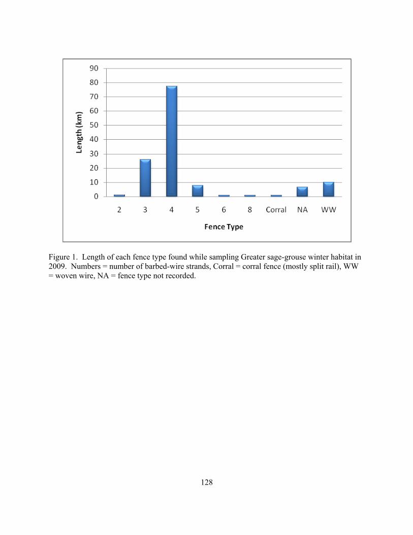
128

Figure 1. Length of each fence type found while sampling Greater sage-grouse winter habitat in 2009. Numbers = number of barbed-wire strands, Corral = corral fence (mostly split rail), WW = woven wire, NA = fence type not recorded.

129

Figure 2. Length of each fence type found while sampling Greater sage-grouse breeding habitat in 2009. Numbers = number of barbed-wire strands, Corral = corral fence (mostly split rail), WW = woven wire, NA = fence type not recorded.

130

Figure 3. Proportion of each type of collision evidence found during 2009 breeding season. FP = feather pile, FIF = feathers in fence, and FIF + FP = both feather piles and feathers in the fence.

131


Micro-habitat use by nesting Greater Sage-Grouse

DAVID D. MUSIL, Idaho Department of Fish and Game, 324 South 417 East, Jerome, ID 83338 USA

ABSTRACT: I investigated nest habitat characteristics for Greater Sage-Grouse (Centrocercus urophasianus) during 2003-2005. I measured vegetation on 156 sage-grouse nests and 138 random plots among 10 meta-populations in southern Idaho. Principal component analysis reduced the set of 89 habitat variables to independent components. The first 3 components described 42% of the variance and included shrub height (23% of variance), shrub density (11%), and horizontal cover (8%). Nests were associated with taller shrubs within 10 m of the nest than available at random and both unsuccessful nests and adult nests had greater shrub height than random plots. No statistical differences could be detected between successful and unsuccessful nests nor between adults and yearlings, but successful yearling nests appeared to have greater horizontal cover than other nests. Nests and random plots in 2005 had greater shrub height than the other 2 years and also had greater horizontal cover. More sites sampled in 2005 were dominated by three-tip sagebrush (Artemisia tripartita) and may have accounted for this difference. A gradient occurs among sites based on moisture zones and shrub height. Xeric/short species of sagebrush have the lowest shrub heights and transition into xeric/tall shrubs and eventually into mesic sites with the tallest shrub heights but least shrub density. Three-tip sagebrush is somewhat intermediate between xeric/tall and mesic sites and has more horizontal cover, but all sites have similar shrub density except for random mesic sites which have lowest shrub densities. Multivariate comparison of means shows nests have less bare rock, greater horizontal cover, taller effective grass height, taller drupe height of live grass and shrubs, and greater shrub canopy cover 1-3 m from the center of the nest than at random plots. Horizontal cover from the perspective of the nesting hen and effective height of grasses were variables not previously used to describe greater sage-grouse nesting habitat but provide additional separation between nest use and random sites.

Key words: Centrocercus urophasianus, Greater Sage-Grouse, horizontal cover, nest habitat, nest use, nest fate.

Greater Sage-Grouse populations have declined throughout the Inter-mountain West (Connelly and Braun 1997, Connelly et al. 2004), and their distribution is greatly influenced by the occurrence of shrub-steppe habitat types, especially those dominated by sagebrush (Patterson 1952, Connelly and Braun 1997). Habitat quality is an important factor influencing nest success, which ultimately affects recruitment and population levels. Eggs in nests are more likely to hatch when sites are under sagebrush (Connelly et al. 1991), have higher canopy coverage and density of sagebrush than the surrounding area (Wallestad and Pyrah 1974), and have greater % cover of residual grass >18 cm tall within 1 m of the nest (Gregg et al. 1994).

132

Past research on greater sage-grouse breeding habitat has focused on shrub structure (Wallestad and Pyrah 1974) and general understory cover (Klebenow 1969, Connelly et al. 1991, Gregg et al. 1994), overlooking the possible importance of horizontal cover and quality of grass cover. Also, past research projects have been conducted on study sites dominated by 1 or 2 sagebrush and grass species. Greater sage-grouse are known to nest in several sagebrush types throughout Idaho (pers. comm. J. Connelly). No research has been conducted to relate plant structure quality or sagebrush species dominance to Greater sage-grouse nest-site use. This information would assist land management agencies to properly manage rangelands to benefit declining greater sage-grouse populations (Schroeder et al. 1999). The objective of this study was to determine vegetation parameters associated with greater sage-grouse nests compared to habitat available at random throughout southern Idaho in areas dominated by a variety of sagebrush and grass species and moisture regimes.

METHODS

This research was conducted on 10 meta-populations (Fig. 1). The populations are distributed throughout southern Idaho ranging in elevation from 1,600-2,400 m in a variety of shrub-steppe habitat types. At least 12 habitat types (Hironaka et al. 1983) are present throughout southern Idaho and at least 1 habitat type is present within each meta population. Habitat type does not necessarily correspond with current dominance by sagebrush and grass species so I categorized a plot based on current conditions and general moisture regimes. Xeric sites have annual precipitation <30 cm/yr whereas Mesic sites have >30 cm annual precipitation. Sagebrush species were categorized as tall (>30 cm including Artemisia tridentata spp and A. tripartita) and short (<30 cm including A. arbuscula, and A. nova).

Nest sites were obtained from radio-marked greater sage-grouse hens monitored as part of other ongoing studies and were considered successful if at least 1 egg hatched. Hens were captured by night lighting (Giesen et al. 1982, Wakkinen et al. 1992b) and fitted with 16.5 g necklace style radio transmitters (Riley and Fistler 1992). Habitat was measured at nest sites after hens ceased nesting efforts or when abandoned or depredated nests would have hatched based on initiation dates and allowing for 27-day incubation (Patterson 1952).

Vegetation sampling was conducted similar to Wakkinen (1990), Gregg et al. (1994), and Musil et al. (1994). Measurements were taken along 4, 10 m transects placed at right angles radiating from the center of the nest and oriented in a random direction. We measured droop height of the closest shrub and grass for each species within 1 m of the transect at 1, 3, and 5 m from the center of the plot for each transect. Droop height is defined as the tallest naturally growing portion of the plant (Connelly et al. 2000, Connelly et al. 2003). Droop height of residual (previous season growth), live (current green and growing blades), flower stalk (tallest of residual or live flower), maximum height (tallest part of entire plant), and number of flower stalks was measured for each grass species separately and averaged. Effective height is measured by placing a meter stick behind the grass or shrub and estimating the tallest height concealing >50 % of the 25 mm wide meter stick.

Horizontal cover outside of the nest bowl was measured with a Robel pole (Robel et al. 1970). The pole is placed at 3 and 5 m from the plot center along the transects and read from 20 cm

133

above the ground immediately outside of the nest shrub or at the center of a random plot (Fig. 2). The view of the pole from this position mimics the point of view of a greater sage-grouse hen incubating a nest. At least one-half of the 2.54 cm tall segment (48 segments/pole) of the pole had to be obscured by vegetation to be counted as covered. Shrub canopy cover (Canfield 1941) and shrub density was measured along the 10 m transects. Gaps in the canopy >5 cm were excluded (Connelly et al. 2003). Shrub density was determined by counting the number of plants of each shrub species touching or within 0.5 m on both sides of the transects. Understory cover for each forb and grass species was measured with a 40 x 50 cm modified Daubenmire (1959) frame at 1, 3, and 5 m from the nest on each of the 4 transects. Cover canopies were modified from Daubenmire (1959) to include more sensitivity for lower cover values. Percent cover classes were: 1 (0-1%), 2 (2-5%), 3 (6-25%), 4 (26-50%), 5 (51-75%), and 6 (76-100%). Slope and aspect were measured using a clinometer and compass, respectively. Elevation was estimated by plotting locations on 7.5-minute quadrangle maps.

Random plots, independent from nest sites, were generated using ArcView Spatial Analyst (ESRI Redlands CA 92373) software and measured during the hatching period. The same measurements made on nests were made at the random plots. Plots were centered on the coordinates, not moved to the nearest sagebrush. Our method of random plot placement was done to eliminate over estimation of shrub canopy cover and density available. Some random plots, if required to be moved to the nearest sagebrush to mimic nest sites, would bias areas with low densities of sagebrush in favor of more dense areas. Shrub canopy and density were measured 1-10 m from the center of the plot and segmented into 1-3, 3-5, and 5-10 m increments to eliminate over-sampling the center.

Principal component analysis (McGarigal et al. 2000) reduced the set of correlated variables to independent components for comparison between nests and random plots. Varimax rotation facilitated interpretation of the variables within the components (O’Rourke et al. 2005). Meaningful factor loadings were set at ±0.40 and I removed variables significantly loading on >1 component and re-running the analysis until complex variables were eliminated. Means were calculated for both principal components and vegetation variables and compared using general linear model comparisons and multivariate analysis of variance, respectively, (O’Rourke et al. 2005) at the 0.05 level of significance.

RESULTS

I measured 156 greater sage-grouse nests and 138 random plots from 12 meta- populations during 2003-2005 in southern Idaho (Fig. 1). Eighty-nine vegetation variables were measured. Forty-four percent (n = 68) of the 156 nests measured were successful. Adults comprised 77% of the nests sampled and of those, 43% were successful whereas 40% of the 35 yearling nests were successful. Overall success of nests sampled was 34% (n = 62), 49% (n = 46), and 44 % (n = 48) in 2003, 2004, and 2005, respectively.

134

Principal Component Analysis

Eleven variables associated with horizontal cover near the ground and live, effective, and maximum grass height were identified as complex variables and were removed from principal component analysis but 78 variables were retained. Sixteen principal components met the minimum Eigenvalue of 1.0 and described 84% of the variance in the data. A majority (55%) of variance was described by the first 5 principal components: shrub height was associated with component I (Prin I, Table 1) and accounted for 23% of the variance, shrub density with component II (Prin II, Table 1) for 11% of variance, horizontal cover (Prin III, Table 1) had 8% of variance, shrub cover (Prin IV) with 7% of variance from 8 variables, and forb cover (Prin V) with 6% of variance from 5 variables.

Nest sites (Fig. 3a) were associated with significantly taller shrubs (P = 0.0019) than available at random but were not different for shrub density (P = 0.1084) or horizontal cover (P = 0.6869). Fates of nests were similar (P > 0.05) to each other for the first 3 principal components (Fig. 3b). Adult nests (Fig. 3c) were associated with significantly taller shrubs than available at random (P = 0.0114) but were similar to yearling nests for all 3 principal components. Nests among age classes and fates were statistically similar to random plots (P = 0.0463) though it appears successful yearlings had greater horizontal cover (Fig. 3d).

Comparing among years, 2005 nest and random sites had significantly greater shrub height (P < 0.0001) and 2005 nests had greater horizontal cover (P < 0.0001) than nest and random plots in 2003 or 2004, but were similar for shrub density (P = 0.0936) and between each other (Fig. 4a).

Grouping plots by 2 categories of moisture regimes (xeric, mesic), 2 categories of shrub growth form (short = Artemisia arbuscula and A. nova, tall = A. tridentata spp.), and 1 category for domination by a single species (three-tip sagebrush Artemisia tripartita), the first 3 principal components showed a gradient from xeric short to mesic (Fig. 4b) for shrub height. Both mesic nests and random plots had greater shrub height (P < 0.001) than all the other categories except for nests dominated by three-tip sagebrush but random mesic plots had less shrub density than xeric/short nests (P = 0.0242). Three-tip sites had greater horizontal cover than xeric and mesic sites and xeric short sites had greater horizontal cover than mesic sites but less than xeric tall sites.

MANOVA Analysis

Multivariate comparisons between means of nest and random plot were compared for 89 variables (Table 2). Nests had less bare rock exposed at the surface than random plots but more horizontal cover. Live grass height at 1, 3, and 5 m from the center and all distances combined were taller at nests than at random plots. Nests also had taller effective grass height at 1 m and for all distances combined. Live shrub height was taller at 1 m from the center for nests as well as flower height at 1 and 3 m from center. Both live and flower heights were taller than random for all distances from the center combined. Nests had greater canopy cover for all shrubs combined at 1-3 m but less sagebrush density at this same distance. Successful and unsuccessful nests were different from random plots, similar to nests vs. random, but were not different among

135

nests. No differences could be detected among adult and yearling nests and random plots (Wilk’s Lambda = 0.41, F = 0.97, P = 0.5492) or among age classes combined with nest fates (Wilk’s Lambda = 0.19, F = 1.15, P = 0.0557). When only nests were compared and random plots omitted, there was no difference detected among age classes and nest fate categories (Wilk’s Lambda = 0.07, F = 0.97, P = 0.5973).

DISCUSSION

Greater sage-grouse hens used nest sites with different structural characteristics than what was available at random in Idaho during 2003-2005. Nests occurred on sites with taller shrubs similar to Sveum et al. (1998) but, contrary to my findings, Aldridge and Brigham (2002) in silver sagebrush (Artemisia cana) habitat found greater shrub density at nests than at random and could not detect a difference in shrub height. Wallestad and Pyrah (1974) found higher density of sagebrush at successful nests than at unsuccessful, but I could not detect differences between nest fates.

Wakkinen (1990) found taller grass at nest sites than at random but he measured only the tallest portion of the plant where I separated grass height among several structures in addition to the maximum height and found taller effective and live grass heights at multiple distances from the plot center. If I had restricted measurements to only maximum grass height, I would have found no differences between nests and random plots and would have erroneously concluded hens were selecting habitat with similar grass structure from what was available at random. It is possible greater soil fertility or moisture content is creating greater live grass growth which the hens are detecting and selecting. Hens may also be choosing areas with less impact by grazing domestic livestock and/or wildlife which is providing more robust grass plants for nest concealment.

Greater sage-grouse hens are likely selecting sites with adequate views of approaching predators (Gotmark et al. 1995) but also for concealment. Hens require concealment while exiting from and returning to the nest during incubation breaks to avoid attracting predators to the nest as well as themselves. Within 6 m surrounding a nest, greater shrub canopy cover provides concealment from aerial predators while greater horizontal cover from taller live and effective grass heights creates obstructing views of the nest from approaching terrestrial predators. Less bare rock provides more potential growing sites for concealment cover. Less shrub density surrounding a nest likely allows a better view of approaching terrestrial predators. Coates (2009) determined yearling hen greater sage-grouse take more frequent and longer incubation breaks than adults thus exposing themselves and their nests to greater depredation. This could explain why successful yearlings tended to have more horizontal cover in my study. Coupling less incubation constancy with apparently less horizontal cover, unsuccessful yearling hens are more exposed during their frequent movements to and from the nest and are more easily detected by predators thus lending themselves to higher nest failure.

Any management practice that drastically reduces cover across a landscape likely minimizes potential use and hatching success by nesting greater sage-grouse. Managers need to realize greater sage-grouse use a variety of sagebrush species and moisture regimes and should identify these landscapes when making landscape altering decisions. Large-scale prescriptions should include a patchwork variety of shrub densities and height structures to adequately provide for all

136

aspects of greater sage-grouse habitat needs. Patterns of habitat use are a mechanism derived by the evolution of the species (Rotenberry 1981) and greater sage-grouse are not likely to adapt quickly enough to changes in vegetation during short time scales. Therefore, it is important to retain habitat characteristics that have been shown to be used by greater sage-grouse as documented by Connelly et al. (2000). Of course, use does not necessarily correlate with fitness at a landscape scale (Aldridge and Boyce 2007).

The 2 habitat measurement methods introduced in this study, effective height and horizontal cover observed from the nesting hen’s perspective, should be tested in other studies to determine their abilities to detect differences in habitat use. Effective height is an alternative to using qualitative categories to describe the robustness of plant structure. Vegetation can have the same height but result in considerably different quality of concealment cover when effective height is measured (Fig. 5). Horizontal cover should be measured at different positions and no more than 2 m from the pole rather than just from the plot center since cover further away is influenced by closer cover. Cover at 5 m was typically masked by cover at 3 m except when cover was lacking at 3 m.

ACKNOWLEDGEMENTS

This research was funded in part by the US Fish & Wildlife Service Federal Aid in Wildlife Restoration Project W-160-R-34. I thank all the Idaho Department of Fish & Game personnel that supervised: J. Connelly and T. Hemker; and worked on this project including the following invaluable field technicians: B. Atkinson, P. Atwood, B. Cadwallader, A. Foley, S. Harrington, D. Lockwood, B. Lowe, R. Morris, C. Perugini, D. Plattner, T. Stirling, D. VanDoren, and R. Wilson. D. VanDoren also suggested the measurement of effective height. I appreciate graduate students N. Burkepile and P. Wik for the use of their nesting hens. G. Stanford, J. Stanford, and B. Tindall were gracious in allowing access to their private land and provided campsites and hospitality for field crews.

LITERATURE CITED

Aldridge, C. L., and M. S. Boyce. 2007. Linking occurrence and fitness to persistence: habitat –based approach for endangered Greater Sage-Grouse. Ecological Applications 17:508-526.

Aldridge, C. L., and R. M. Brigham. 2002. Sage-Grouse nesting an brood habitat use in southern Canada. Journal of Wildlife Management 66:433-444.

Canfield, R. H. 1941. Application of the line interception method in sampling range vegetation. Journal of Forestry 39:388-394.

Coates, P. S. and D. J. Delehanty. 2009. Effects of environmental factors on incubation patterns of Greater Sage-Grouse. Condor 110:627-638.

Connelly, J. W., W. L. Wakkinen, A. D. Apa, and K. P. Reese. 1991. Sage-Grouse use of nest sites in southeastern Idaho. Journal of Wildlife Management 55:521-524.

137

Connelly, J. W. and C. E. Braun. 1997. Long-term changes in sage grouse Centrocercus urophasianus populations in western North America. Wildlife Biology 3:229-234.

Connelly, J. W., M. A. Schroeder, A. R. Sands, and C. E. Braun. 2000. Guidelines to manage sage grouse populations and their habitats. Wildlife Society Bulletin 28:967-985.

Connelly, J. W., K. P. Reese, and M. A. Schroeder. 2003. Monitoring of Greater Sage-Grouse habitats and populations. Bulletin 80 University of Idaho, College of Natural Resources Experiment Station , Moscow, USA.

Connelly, J. W., S. T. Knick, M. A. Schroeder, and S. J. Stiver. 2004. Conservation Assessment of Greater Sage-Grouse and Sagebrush Habitats. Western Association of Fish and Wildlife Agencies. Unpublished Report. Cheyenne, Wyoming.

Daubenmire, R. 1959. A canopy-coverage method of vegetational analysis. Northwest Science 33:43-64.

Gotmark, F., D. Blomqvist, O. C. Hohansson, and J. Bergkvist. 1995. Nest site selection: A trade-off between concealment and view of the surroundings? Journal of Avian Biology 26:305-312.

Gregg, M. A., J. A. Crawford, M. S. Drut, and A. K. DeLong. 1994. Vegetational cover and predation of Sage-Grouse nests in Oregon. Journal of Wildlife Management 58:162-166.

Giesen, K. M., T. J. Schoenberg, and C. E. Braun. 1982. Methods for trapping sage grouse in Colorado. Wildlife Society Bulletin 10:224-231.

Hironaka, M., M. A. Fosberg, and A. H. Winward. 1983. Sagebrush-grass habitat types of southern Idaho. College of Forestry, Wildlife, and Range Sciences Bulletin Number 35. Moscow, ID.

Klebenow, D. A. 1969. Sage-Grouse nesting and brood habitat in Idaho. Journal of Wildlife Management 33:649-662.

McGarigal, K., S. Cushman, and S. Stafford. 2000. Multivariate statistics for wildlife and ecology research. Springer-Verlag, New York, New York, USA.

Musil, D. D., K. P. Reese, and J. W. Connelly. 1994. Nesting and summer habitat use by translocated Sage-Grouse (Centrocercus urophasianus) in central Idaho. Great Basin Naturalist 54:228-233.

O’Rourke, N., L. Hatcher, and E. J. Stepanski. 2005. A step-by-step approach to using SAS for univariate and multivariate statistics. Second Edition. SAS Institute, Inc., Cary, North Carolina, USA.

138

Patterson, R. L. 1952. The Sage-Grouse in Wyoming. Sage Books, Inc., Denver, Colorado, USA.

Riley, T. Z. and B. A. Fistler. 1992. Necklace radio transmitter attachment for pheasants. Journal of Iowa Academy of Science 99:65-66.

Robel, R. J., J. N. Briggs, A. D. Dayton, and L. C. Hulbert. 1970. Relationships between visual obstruction measurements and weight of grassland vegetation. Journal of Range Management 23:295.

Rotenberry, J. T. 1981. Why measure bird habitat? Pages 29-32 in D. E. Capen, editor. The use of multivariate statistics in studies of wildlife habitat. General Technical Report RM-87, Rocky Mountain Forest and Range Experiment Station, Fort Collins, Colorado, USA.

Schroeder, M. A., J. R. Young, and C. E. Braun. 1999. Sage Grouse (Centrocercus urophasianus). In A. Poole and F. Gill [EDS.], The birds of North America, No. 425. The Birds of North America, Inc., Philadelphia, PA.

Sveum, C. M., W. D. Edge, and J. A. Crawford. 1998. Nesting habitat selection by Sage-Grouse in south-central Washington. Journal of Range Management 51:265-269.

Wakkinen, W. L. 1990. Nest site characteristics and spring-summer movements of migratory Sage-Grouse in southeastern Idaho. Thesis, University of Idaho, Moscow, USA.

Wakkinen, W. L., K. P. Reese, and J. W. Connelly. 1992a. Sage Grouse Nest Locations in Relation to Leks. Journal of Wildlife Management 56:381-383.

Wakkinen, W. L., K. P. Reese, and J. W. Connelly, and R. A. Fischer. 1992b. An improved spotlighting technique for capturing sage grouse. Wildlife Society Bulletin 20:425-426.

Wallestad, R. O. and D. B. Pyrah. 1974. Movement and nesting of sage grouse hens in central Montana. Journal of Wildlife Management 38:630-633.

139

Table 1. Variables associated with the first 3 principal components for greater sage-grouse nest habitat in Idaho, US, 2003-2005

____________________________________________________________________________________________________________________________________________________________ Principal Component I Principal Component II Principal Component III ______________________________________________________________________________ Shrub live height 1 m Density shrubs 1-3 m Horizontal cover ground level 3 m Shrub effective height 1 m Density shrubs 3-5 m Horizontal cover high height 3 m Shrub live height 3 m Density shrubs 5-10 m Horizontal cover medium height 3 m Shrub effective height 3 m Density shrubs 1-10 m Horizontal cover total height 3 m Shrub live height 5 m Density sagebrush 1-3 m Horizontal cover low height 5 m Shrub effective height 5 m Density sagebrush 3-5 m Horizontal cover medium height 5 m Shrub live height total Density sagebrush 5-10 m Horizontal cover high height 5 m Shrub effective height total Density sagebrush 1-10 m Horizontal cover total height 5 m ______________________________________________________________________________ Note: Distance values are distances from center of plot, eg. 5-10 m are measurements taken from segment of plot 5-10 m from center.

140

Table 2. Vegetation characteristics at greater sage-grouse nest sites and available at random, Idaho, 2003-2005

________________________________________________________________________________________________________________________________________________ Nests (n = 156) Random (n = 138) Variable Mean SD Mean SD P ________________________________________________________________________ Grass % Cover # of species 3.7 1.2 3.4 1.4 0.0485 1 ma 22.9 15.0 20.3 15.1 0.1426 3 m 20.8 13.8 20.2 14.5 0.7109 5 m 22.1 14.5 19.6 14.3 0.1462 total 21.9 13.4 20.0 13.8 0.2350 Cheatgrass cover total 2.9 6.3 3.0 7.0 0.9054 Crested wheatgrass cover total 0.9 4.2 0.9 4.9 0.8569 Forb % Cover # of species 8.0 4.6 7.2 5.2 0.1506 1 m 11.4 12.1 11.1 11.9 0.8297 3 m 11.7 12.0 10.9 12.7 0.5474 5 m 12.6 13.2 11.0 11.4 0.2702 total 11.9 11.4 11.0 11.2 0.4852 Rock % Cover 1 m 7.5 11.5 14.4 19.1 0.0002 3 m 10.3 15.7 14.7 18.8 0.0319 5 m 10.9 16.2 15.3 18.8 0.0317 total 9.6 13.9 14.8 18.0 0.0053 Horizontal % Cover 3 m from center totalb 53.3 25.9 40.0 23.0 <0.0001 low 93.8 11.3 85.8 19.4 <0.0001 ground 72.1 22.3 60.3 27.0 <0.0001 medium 63.1 28.6 49.8 32.5 0.0002 high 34.5 32.7 17.7 22.8 <0.0001 5 m from center total 65.3 24.1 52.4 26.4 <0.0001 low 98.3 5.2 93.7 14.1 0.0002 ground 84.2 17.7 73.2 26.5 <0.0001 medium 78.5 23.7 64.8 32.2 <0.0001 high 46.3 33.7 31.6 30.7 0.0001

Table 2 Continued

141

Grass Height (cm) # of species 4.2 1.5 4.0 1.6 0.2761 1 m from center residual 12.1 9.3 10.3 10.8 0.1382 live 17.2 7.3 13.9 6.3 <0.0001 flower 25.1 13.9 24.0 11.5 0.4889 # flower stalks/plant 4.8 7.7 4.2 5.8 0.4168 effective 9.0 6.7 7.5 5.3 0.0368 maximum 27.2 12.2 25.4 12.3 0.2059 3 m from center residual 12.9 10.3 10.7 12.4 0.0971 live 16.6 7.2 14.3 6.1 0.0025 flower 24.4 12.9 24.6 11.1 0.9008 # flower stalks/plant 4.4 7.3 4.4 6.0 0.9562 effective 8.9 7.4 7.8 5.0 0.1356 maximum 26.9 12.3 25.9 13.7 0.5430 5 m from center residual 11.7 8.1 10.3 9.1 0.1520 live 16.2 7.1 13.9 5.5 0.0022 flower 24.9 13.1 24.4 10.9 0.6968 # flower stalks/plant 5.3 8.7 4.1 5.0 0.1435 effective 8.2 5.1 7.7 5.1 0.4082 maximum 27.0 11.1 25.6 10.8 0.3065 Total residual 12.2 8.6 11.1 10.7 0.3203 live 16.4 6.8 14.1 5.4 0.0019 flower 26.6 13.4 25.4 9.6 0.4058 # flower stalks/plant 5.3 8.8 4.4 5.9 0.3126 effective 10.2 9.9 8.1 6.3 0.0279 maximum 31.8 12.8 30.0 13.4 0.2286 Shrub Height (cm) # species 3.0 1.9 2.8 1.8 0.3922 1 m from center live 43.0 23.1 36.4 26.2 0.0237 flower 40.1 33.0 28.5 37.5 0.0052 # flower stalks/plant 36.6 67.3 25.6 93.5 0.2429 effective 36.5 25.3 30.7 27.4 0.0645 3 m from center live 39.5 17.3 36.6 20.9 0.1938 flower 38.4 29.2 29.4 29.1 0.0092 # flower stalks/plant 28.7 42.5 24.8 60.1 0.5255 effective 32.7 18.6 30.5 22.0 0.3537 5 m from center live 39.4 19.2 35.8 21.5 0.1304 flower 35.7 28.4 29.5 40.2 0.1231

Table 2 Continued

142

# flower stalks/plant 31.1 49.4 25.0 62.7 0.3484 effective 30.8 19.9 29.5 22.5 0.6006 Total live 41.3 18.9 36.5 21.0 0.0364 flower 41.2 29.7 32.0 32.5 0.0119 # flower stalks/plant 31.8 44.1 24.9 66.7 0.2945 effective 32.6 20.1 30.5 22.3 0.4035 Shrub Canopy % Cover # species 3.6 1.5 3.4 1.5 0.1645 shrubs 1-3 mc 23.4 15.4 19.3 14.1 0.0186 shrubs 3-5 m 22.9 15.6 21.0 14.6 0.3003 shrubs 5-10 m 21.5 13.1 19.6 13.0 0.2062 shrubs 1-10 m 22.2 13.0 19.8 12.7 0.1119 sagebrush 1-3 m 13.9 11.2 12.1 11.2 0.1773 sagebrush 3-5 m 14.8 12.2 13.4 11.8 0.3164 sagebrush 5-10 m 13.3 9.2 12.5 9.4 0.4375 sagebrush 1-10 m 13.8 9.1 12.6 9.2 0.2721 Shrub Density (#/m2) # species 4.0 1.7 3.9 1.7 0.3407 shrubs 1-3 m 2.8 1.8 3.0 2.5 0.2506 shrubs 3-5 m 3.1 3.3 3.2 2.5 0.8780 shrubs 5-10 m 2.8 2.3 2.8 1.9 0.9397 shrubs 1-10 m 2.9 2.3 2.9 2.1 0.7379 sagebrush 1-3 m 1.6 1.3 2.0 2.0 0.0562 sagebrush 3-5 m 2.0 3.0 2.1 2.0 0.8703 sagebrush 5-10 m 1.8 2.0 1.9 1.6 0.5902 sagebrush 1-10 m 1.8 2.0 2.0 1.7 0.4720 Slope (degrees) 5.2 6.0 4.1 4.8 0.0993 Aspect (degrees azimuth) 167.7 105.9 160.0 103.1 0.5308 Elevation (m) 1633.1 249.3 1664.7 251.7 0.2812 ________________________________________________________________________ a Cover measurements taken at 1, 3, and 5 m from center of plot in 4, 900 directions. b Cover measured with Robel pole: total cover measured 0-122 cm above ground, low cover 0-18 cm, ground 0-61, medium 19-61 cm, and high 62-122 cm. c Canopy cover measured with line intercept at segments 1-3, 3-5, and 5-10 m from center of plot in 4, 900 directions. Shrubs includes all shrub species, sagebrush is only for sagebrush species. Note: Multiple comparisons protected by results of MANOVA; Wilk’s Lambda = 0.58, F = 1.67, P = 0.0016.

143

Figure 1. Meta-populations sampled for Greater sage-grouse nests in southern Idaho, US, 2003-2005. Numbers within markers are sample sizes for nests. Shaded area depicts Greater sage-grouse distribution.

144

Figure 2. Measurement of horizontal cover at a Greater sage-grouse nest site, Idaho, US. Photo A: observer reading Robel pole from immediately outside the nest bowl with eye level 20 cm above ground. Pole is 3 m distance from center of nest. Photo B: view of Robel pole measured in Photo A.

145

Figure 3. Habitat relationship of first 3 principal components for Greater sage-grouse nests and random plots in Idaho, US, 2003-2005. A) Greater sage-grouse nest sites and random plots, b) fate of nests, c) age of nesting hen, and d) age of hen and fate of nest.

146

Figure 4. Habitat relationship for first 3 principal components among Greater sage-grouse nest sites and random plots by a) year and b) based on moisture content and shrub size in Idaho, US, 2003-2005.

147

Figure 5. Comparison between 2 grass plants with similar heights but different quality of cover based on “effective height”. Grass on left has more effective horizontal cover and number of flower stalks than the grass on the right but both have relatively identical droop height measurements of residual, live, and flower height.

148

STUDY II: Population Characteristics and Habitat Use of Exploited Forest Grouse Populations


ABSTRACT: Forest grouse (dusky grouse [Dendragapus obscurus], ruffed grouse [Bonasa umbellus], and spruce grouse [Falcipennis canadensis]), are increasing in popularity among gamebird hunters in Idaho. Unfortunately, abundance, population trends, and harvest rates are largely unknown in the state. Twelve line transects and 2 roadside surveys have been sampled for ruffed and dusky grouse during the last 3 years in the Squaw Creek drainage of game management unit 32A. Nineteen ruffed grouse males have been captured, radio-collared, and monitored for survival and movements.

KEYWORDS: Forest grouse, ruffed grouse, dusky grouse, spruce grouse, surveys, counts, transects

Forest grouse (ruffed grouse [Bonasa umbellus], dusky grouse [Dendragapus obscurus], and spruce grouse [Falcipennis canadensis]), are among the most popular game birds in Idaho, annually averaging 148,000 harvested birds (1990-2006) and averaging 23% of the upland game bird harvest, second highest of all species (IDFG 2007). Unfortunately, abundance (density), population trends, and harvest rates (portion of population being harvested) are largely unknown. Forest grouse are also dependent on habitat often affected by land management decisions (e.g., riparian zones, mixed shrub uplands, and older growth timber). To properly manage these game birds and assess responses to habitat change and harvest by hunters, reliable survey techniques need to be developed and tested. In Idaho, no standardized routes are monitored before the hunting season to track population trends or forecast harvest. Forest grouse populations in close proximity to urban areas or other landscape features (e.g. roads) may have higher harvest rates than more remote populations. Also, forest management is changing to increase health of stands and prescriptions to reduce threats of wildfire, both of which may impact forest grouse.

As forest grouse become more popular as a hunted game species because other upland species are declining, determining accurate population levels is critical for proper management. Currently, Idaho relies on incidental pre-hunting season observations by biologists and conservation officers to estimate population trend and to forecast harvest opportunity for hunters. Eastern states with ruffed grouse monitor population trends with spring drumming counts and assume a 1:1 male to female ratio. This estimate is prior to nesting and does not reflect summer weather affecting chick survival. Occasionally, Idaho has monitored drumming routes but these have not been consistent or standardized. No standardized surveys have been conducted in Idaho for dusky or spruce grouse.

Historically, the forest grouse hunting season length in Idaho was conservative (mid-September to end of November). During the 1980s, the seasons gradually increased to the current length started in 1990 (1 September – 31 December). It is unknown if this has had an effect on the harvest of hens with broods but has been speculated as the cause for reductions in populations of ruffed grouse in areas close to urban centers. The daily bag and possession limits have been held constant at 4 birds/day, 8 birds in possession in aggregate. It is unknown if the 3 species of

149

forest grouse in Idaho are affected by this harvest strategy. Devers et al. (2007) present a thorough review of effects of harvest on forest grouse, mainly ruffed grouse and dusky grouse, and found equivocal evidence. Hunting may be compensatory up to a certain point, then become additive but depends on several factors including landscape attributes and hunter behavior. Monitoring harvest rates in Idaho will be critical to determine hunting pressure on the different species and age/sex classes.

STUDY AREA

The Second Fork of Squaw Creek is within the Boise National Forest in Gem County of west central Idaho. The study area is dominated by ponderosa pine (Pinus ponderosa) with patches of quaking aspen (Populus tremuloides) Open areas are dominated by sagebrush (Artemisia tridentata) and antelope bitterbrush (Purshia tridentata). Riparian zones are dominated by currants (Ribes spp), chokecherry (Prunus virginiana) and hawthorn (Crataegus spp.). The study area has a west-southwest aspect and elevation ranges 1160-1524 m. Two main gravel roads, FS 653 and FS 626, provide access to the Second Fork and Sage Hen Reservoir drainages, respectively. Many 2-track logging roads intersect the main roads.

METHODS

Capture and Marking

We used a walk-in trap with similar dimensions to Gullion (1965) but constructed ours of plastic drainpipe rather than a wooden frame wrapped in hardware cloth. Traps were deployed on active drumming logs found during line transect and roadside surveys. Traps were checked twice daily by 1000 and 2100 hrs. Necklace style (Riley and Fistler 1992) 12 g radio transmitters <2% of grouse body mass (Kenward 1987) were used and programmed with 4 hour mortality sensors (Advanced Telemetry Systems, Isanti, MN 55040). Birds were also weighed with 1000 g spring scales. Telemetry was conducted with a 3 element collapsible Yagi antenna and locations determined by visual observation, flushes, or circling the location within a 30-50 m radius.

Roadside indices

Roadside surveys for displaying male forest grouse were conducted April – June depending on access conditions. Routes are at least 5 km long, started half hour before sunrise, and end <2 hours after sunrise. Observation points are at 800 m intervals and observed for 5 minutes per stop. Stops are spaced to avoid overlap of observations if roads or trails switchback due to topography. Routes are not run when wind is >15 km/hr or precipitation is heavy.

Point intersection transect surveys

Random start points were generated within the study areas using ArcGIS (ESRI, Redlands, CA) and spaced 400 m apart. Random directions (azimuth) for each transect were generated and spaced >400 m from the nearest transect. Transects are 1000 m in length and marked with surveyor flagging at each observation point spaced 100 m apart for 11 points along the transect. Each transect was run from half hour before sunrise to 2 hours after sunrise. Transects were conducted with the same weather protocol as for roadside surveys.

150

The same transects were used in 2009 to survey brood rearing female ruffed grouse by playing a recording of a chick distress call. We also attempted to noosepole females but were unsuccessful. We played the calls for 4-5 minutes similar to Healy et al. (1980).

Hunter surveys

Mandatory check stations will be conducted at the intersection of Second Fork Squaw Creek and Sagehen Reservoir Road. Opening day and weekend will be surveyed while subsequent weekdays and weekends will be randomly stratified with 20% of the weekdays and 50% of the weekends sampled. Opening days and weekends of big game seasons will also be targeted for check stations. Check stations will be operated from 1000 to 1930 - traditional survey hours used in past management check stations in Idaho.

RESULTS

Ruffed grouse drumming surveys were established on 12 line transects and 2 roadsides. Three line transects, intentionally run along creek drainages (#15, #70, #88) in 2007 were changed to random directions in 2008 to comply with line transect protocal (Buckland et al. 2001). Two roadside surveys were conducted on 2 separate roads (FS 653 and FS 626). Assuming drumming males can be heard up to 200 m (Gullion 1966, Zimmerman and Gutierrez 2007), we estimated ruffed grouse density in 2007 to be 4.5 and 6.5 drumming males/km2 for line transects and roadside surveys, respectively. Data from 2008 and 2009 have not been analyzed.

Eight walk-in traps were used to capture 19 drumming male ruffed grouse during 2007-2009. Survival estimates, movements, and home ranges have not been estimated for the 2008-2009 data. For 2007, 6 males averaged 559 + 41 g with a dispersal of 175 + 57 m from capture site and an average home range (minimum convex polygon) of 22.7 + 11.2 ha. Rough estimates for the 2008-2009 males will be quite similar.

DISCUSSION

Density of drumming male ruffed grouse in our study area appears to be similar to low cycles in British Columbia (Davies and Bergerud 1988) and within the ranges, but slightly lower than average to those across North America (Rusch et al. 2000).

Additional funding was pursued via non-profit grants but was unsuccessful to increase the budget of this project. Currently, most of the upland gamebird budget is directed towards greater sage-grouse (Centrocercus urophasianus) and mountain quail (Oreortyx pictus).

151

LITERATURE CITED

Buckland, S. T., D. R. Anderson, K. P. Burnham, J. L. Laake, D. L. Borchers, and L. Thomas. 2001. Introduction to distance sampling estimating abundance of biological populations. Oxford University Press, Inc., New York, USA.

Davies, R. G. and A. T. Bergerud. 1988. Demography and behavior of ruffed grouse in British Columbia. Pages 78-121 in A. T. Bergerud and M. W. Gratson, editors. Adaptive strategies and population ecology of northern grouse. University of Minnesota Press, Minneapolis, Minnesota, USA.

Devers, P. K., D. F. Stauffer, G. W. Norman, D. E. Steffen, D. M. Whitaker, J. D. Sole, T. J. Allen, S. L. Bittner, D. A. Buehler, J. W. Edwards, D. E. Figert, S. T. Friedhoff, W. W. Giuliano, C. A. Harper, W. K. Igo, R. L. Kirkpatrick, M. H. Seamster, H. A. Spiker, Jr., D A. Swanson, and B. C. Tefft. 2007. Ruffed grouse population ecology in the Appalachian region. Wildlife Monographs 168,1-36.

Gullion, G. W. 1965. Improvements in methods for trapping and marking ruffed grouse. Journal of Wildlife Management 29:109-116.

_______. 1966. The use of drumming behavior in ruffed grouse population studies. Journal of Wildlife Management 30:717-729.

Healy, W. M., R. O. Kimmel, D. A. Holdermann, and W. Hunyadi. 1980. Attracting ruffed grouse broods with tape-recorded chick calls. Wildlife Society Bulletin 8:69-71.

Idaho Department of Fish and Game. 2007. Upland game progress report. Study II, Job 1. Project W-170-R-31.

Kenward, R. 1987. Wildlife radio tagging – equipment, field techniques, and data analysis. Academic Press, New York, USA.

Riley, T. Z. and B. A. Fistler. 1992. Necklace radio transmitter attachment for pheasants. Journal of Iowa Academy of Science 99:65-66.

Rusch, D. H., S DeStefano, M. C. Reynolds, and D. Lauten. 2000. Ruffed grouse (Bonasa umbellus). in A. Poole and F. Gill, editors. The birds of North America, No. 515. The Birds of North America, Inc., Philadelphia, Pennsylvania, USA.

Zimmerman, G. S. and R. J. Gutiérrez. 2007. The influence of ecological factors on detecting drumming ruffed grouse. Journal of Wildlife Management 71:1765-1772

152

Study III: Translocation of mountain quail into historic habitats

Mountain Quail: movement, survival, reproduction, habitat use and abiotic effects in the Bennett Hills, ID.

GIFFORD L. GILLETTE Department of Biological Sciences, 921 S. 8th Avenue, Stop 8007, Idaho, State University, Pocatello, ID 83209, USA

DAVID J. DELEHANTY, Department of Biological Sciences, 921 S. 8th Avenue, Stop 8007, Idaho, State University, Pocatello, ID 83209, USA

JOHN W. CONNELLY, Department of Biological Sciences, 921 S. 8th Avenue, Stop 8007, Idaho, State University, Pocatello, ID 83209, USA

ABSTRACT. We predicted that mountain quail (Oreortyx pictus) released at a xeric, low-elevation site would move further and have a lower survival rate than a mesic, high-elevation release site. We implemented a new trapping technique to monitor birds beyond the traditional spring-summer season and through autumn and winter and predicted variation in survival during winter would be contingent upon prevailing winter conditions. Our objectives included; monitoring the movements, reproduction, and survival of a founding population of quail for 2 years. Objectives also included directly testing some of the conflicting hypotheses explaining variation in mountain quail survival during the breeding-brooding season, and providing basic life-history information, including dispersal distances, age-specific mortality, and lifespan. Our study area encompasses approximately 63,000 ha within the Bennett Hills located about 70 km southeast of Boise, Idaho. Mountain quail released at the low-elevation site on average moved 5 km farther than quail at the high-elevation release site; nonetheless, post release movement did not influence survival of mountain quail. Kaplan Meier survival estimates were similar between release sites throughout the 150-day breeding-brooding season in 2008. Trapping efforts in late summer enabled us to monitor beyond the traditional 150-day spring and summer field season and we observed that survival rates averaged 96% during autumn 2007 and 2008.

KEYWORDS: Idaho, Mountain quail, movements, Oreortyx pictus, reproduction, survival

Understanding population dynamics requires knowledge of how survival and reproduction varies across the lifespan of an individual (Cole 1954). Biotic and abiotic factors differentially affect survival of organisms living in a seasonal environment (Carlson and Letcher 2003). Relating seasonal variation in biotic and abiotic factors to seasonal variation in survival is common for some species (Letcher et al. 2002, Mitro and Zale 2002, Carlson and Letcher 2003) but rare for mountain quail (Oreortyx pictus). Most mountain quail studies are conducted for 150 days – beginning in early spring and ending in late summer when transmitter batteries fail. Observing the number of individuals that survive to reproduce is a good short-term indicator of translocation success (Scott and Carpenter 1987); however, only a few studies have reported survival during autumn and winter (Delehanty 1997, Reese et al. 1999, Pope 2002). Most recent information concerning population dynamics of mountain quail includes only survival and reproduction during spring and summer.

153

There is considerable variation in survival within the breeding and brooding season for mountain quail. Nelson (2007) reported the first 2 weeks prior to release explained 75% of survival across this 150-day monitoring period. Survival rates have varied from 15% (Stephenson 2008) to 72% (Herman et al. 2002) during the breeding-brooding season. Stephenson (2008) reported low survival rates (approximately 20%) for mountain quail released in Western Idaho and Eastern Washington and noted a negative correlation between movement rate and survival. One of the few consistent trends is that mountain quail survive well during incubation periods and late summer (Stephenson 2008, Nelson 2007, Troy 2007).

Most hypotheses explaining the cause for variation in survival of mountain quail invoke predation by raptors (Pope 2002, Stephenson 2008, Nelson 2007). This hypothesis has not been tested directly. We hypothesize that survival rates vary significantly from year-to-year during autumn and winter for mountain quail because this species possesses many characteristics of an r-selected species. Pope (2002) proposed that irruptive population changes may go undetected in year-to-year comparisons of survival; hence, documenting long-term population trends would be valuable (Nelson 2007). Furthermore, proximate factors indirectly related to predation such as predator abundance, habitat condition, and anti-predator behaviors have not been adequately studied (Pope 2002) for mountain quail.

We had 2 release sites that differed topographically and edaphically and tested if those differences affected mountain quail movements and, in turn, survival rates. We predicted that birds released at a xeric, low-elevation site (1500 m) would move further and have a lower survival rate than a mesic, high-elevation release site (1750 m). We implemented a new trapping technique to monitor birds beyond the traditional spring-summer season and through autumn and winter. We predicted variation in survival during winter contingent upon the prevailing winter conditions. Our objectives included; monitoring the movements, reproduction, and survival of a founding population of quail for 2 years, directly testing some of the conflicting hypotheses explaining variation in mountain quail survival during the breeding-brooding season, providing basic life-history information lacking for mountain quail, including dispersal distances, age-specific mortality, and lifespan.

STUDY AREA

The restoration of mountain quail began in spring 2006 (Troy et al. 2007). This study is a continuation of that project. Releases took place in spring 2008 and 2009 on the Bennett Hills. The Bennett Hills are located about 70 km southeast of Boise, Idaho. The elevation ranges from 900 to 2300 m. The study area encompasses approximately 63,000 ha and is a wildlife migration corridor for many species inhabiting the Sawtooth National Forest of the northern US Rocky Mountains. The annual precipitation ranges from 23 to 40 cm and annual snowfall ranges from 90 to 130 cm.

There were 2 different release sites on the Bennett Hills. Site 1 was adjacent to Bennett mountain road (Easting – 634869, Northing – 4783556, Universal Transverse Mercator WGS 84) and site 2 was approximately 20 km east on the west fork of Dempsey creek (Easting – 653905 Northing – 4778959 Universal Transverse Mercator WGS 84). Site 1 is approximately 250 m higher in elevation than site 2. There are more springs, streams, and cover types at site 1 than

154

site 2 within a 5-km radius. The additional cover type was Douglas fir at site 1, whereas the closest conifer cover type is approximately 6 km from site 2. The permanence of watercourses is greater at site 1 than site 2, with drainages dominated by perennial as opposed to ephemeral streams.

Predators in the Bennett Hills include the gray wolf (Canus lupus), black bear (Ursus americanus), golden eagle (Aquila chrysaetos), gray fox (Vulpes velox), mountain lion (Puma concolor), wolverine (Gulo gulo), badger (Taxidea taxus), bobcat (Lynx rufus), pine marten (Martes americana), red-tailed hawk (Buteo jamaicensis), swainson’s hawk (Buteo swainsoni), prairie falcon (Falco mexicanus) and all 3 of the Accipiter genera: sharp-shinned hawk (Accipiter striatus velox), Cooper’s hawk (Accipiter cooperii), and the goshawk (Accipiter gentilis). Introduced species of Galliformes include the California quail (Callipepla californica), ring-necked pheasant (Phasianus colchicus), gray partridge (Perdix perdix), and chukar (Alectoris chukar).

Low elevations are xeric with few springs and perennial streams; the dominant terrain consists of large plateaus of igneous rock dissected by narrow, steep canyons (Bishop et al. 2005) with ephemeral streams. Low elevations are composed of shrub-steppe except in areas of disturbance, which have converted to annual grassland. Major habitat types include big sagebrush (Artemisia tridentata), antelope bitterbrush (Purshia tridentata), blue-bunch wheatgrass (Pseudoroegneria spicata), and cheatgrass (Bromus tectorum). Other less common plants include serviceberry (Amelanchier alnifolia), rabbitbrush (Chrysothamnus nauseosus), fern-leaved desert-parsley (Lomatium dissectum), low sagebrush (Artemesia arbusculus), and buckwheat (Eriogonum sp.). Some riparian woodland exists at low elevations.

High elevations are mesic with many springs and perennial streams; the dominant terrain consists of steep slopes and basalt outcrops. Open ridges are covered with shrub steppe, draw bottoms are lined with deciduous shrubs, and north-facing slopes contain coniferous forest and deciduous shrubs. Major habitat types include a mosaic of big sagebrush, antelope bitter brush, snowbrush (Ceanothus velutinis), choke cherry (Prunus virginiana), bitter cherry (Prunus emarginata) and Douglas fir (Pseudotsuga menziesii). Other less common plants include snowberry (Symphoricarpos albus), rocky mountain maple (Acer glabrum), buckwheat (Eriogonum), quaking aspen (Populus tremuloides), blue-bunch wheatgrass, and cheat grass.

METHODS

Captive Conditions and Release

Mountain quail were captured by a private trapper contracted through the Oregon Department of Fish and Wildlife in late autumn and early winter using funnel traps. Mountain quail were captured in the Cascade and Coastal ranges of western Oregon and held in captivity in Roseburg, Oregon until their transfer to an ALAAC certified aviary on the campus of Idaho State University Pocatello, Idaho.

We fitted Mountain quail with 4.6 g necklace-style radio transmitters (RI-2BM Holohil, Inc.), less than 2% of the average body weight. In 2008, mountain quail were released on 1 May at site

155

1, and 2 May at site 2. We released 22 mountain quail equipped with radio-transmitters at site 1, and 48 mountain quail, of which 23 were equipped with radio-transmitters at site 2. In 2009, releases took place at both sites on 24 April. We released 39 birds of which 23 were equipped with radio-transmitters at each site. In 2008, no uncollared mountain quail were released at site 2 in an effort to detect the establishment of a nascent population as well as detect differences in survival, movement, and reproduction as a function of social differences between release sites. We controlled for age by only fitting birds with radio-transmitters that were hatch-year birds. Release date was contingent upon accessibility to release site with all-terrain vehicles and after forbs and grasses had begun to sprout.

Capture and Radiotelemetry

A variety of fixed-wing airplanes, four-wheel drive vehicles, and all-terrain vehicles were used to access remote areas that mountain quail inhabited. In the first and second months of the translocation, aerial surveys were conducted every 2 weeks and once a month thereafter for the remainder of the breeding-brooding season. Mountain quail were monitored close enough to determine whether reproductive efforts were successful but not to the point where birds were disturbed. On average, birds were located every 4 days or twice a week through ground and aerial radiotelemetry for 150 days post release. For example, of the 2 locations per week one was a specific location accompanied with a visual of the bird while the other location was a more general location indicating a particular drainage occupied by the bird. Upon specific location of a mountain quail, we collected information regarding elevation (m), slope (%), aspect (degrees), habitat type, distance from release site (m), and distance to surface water (m). We used aerial telemetry to locate birds that we could not find on the ground. Mortality signal transmitters helped minimize disturbing birds and at the same time monitor their status.

We trapped mountain quail in September, October, and November during the new moon as weather conditions permitted using a night-netting technique described by Troy et al. (in review). Mountain quail were located using radiotelemetry and spotlights. Upon location, the final capture attempt consisted of using a modified net with a light mounted inside the rim of the net to penetrate thick brush that mountain quail roost in. Once mountain quail were captured, the original radio-transmitter was replaced with a new radio-transmitter.

Reproduction and Vegetation Cover Use

We monitored number of nests incubated by collared birds, number of eggs laid and hatched, approximate incubation length of time, nest success, brood success, and brood habitat use. To avoid causing mountain quail to abandon nest sites, once a bird was found incubating a nest we waited at least 2 weeks before flushing her off the nest to obtain an egg count.

Nest habitat and vegetations surveys conducted were consistent with protocol established by Pope (2002) and adapted by other mountain quail studies (Reese et al. 2005, Nelson 2007, Stephenson 2008). After mountain quail successfully fledged their young and left the area near the nest, we conducted vegetation and habitat surveys at the nest. Each nest site analysis was accompanied with a random location. The random location was determined by taking a random compass bearing and distance between 25-200 m from the corresponding true nest site but within

156

the same cover type. Visual obstruction was measured using a 3 m tall and 3 cm wide robel pole (Robel et al. 1970) with alternating decimeters marked black and white. The robel pole was placed in the nest bowl and viewed 4 m and 8 m from the nest in each of the cardinal directions at a height of 1 meter. Understory was measured using a 20 x 50 cm Daubenmire frame (Daubenmire 1959) centered on the nest bowl and at 2 m and 4 m in each cardinal direction for a total of 9 measurements per site. The species and height of the tallest and shortest shrub within 1 meter of the nest and 4 m from the nest in each of the cardinal directions were recorded.

Statistical Analysis

Movement data did not have a normal distribution and variances were not equal; therefore, a permutation test or Wilcoxon Mann-Whitney Rank Sum Test in Program R was used to test for differences in movement between sites (R-Statistics 2004). Survival estimates for the breeding-brooding season were calculated with the Kaplan Meier method (Kaplan and Meier 1958, Pollock et al. 1989). Data for snowpack were obtained from the USDA Natural Resources Conservation Sources. They collect data at the end of December, January, February, and March (http://www.wcc.nrcs.usda.gov) at 3 different sites we refer to as low (1200 m), medium (1350 m), and high (1525 m) elevation in the Bennett Hills.

RESULTS

Movement

We documented a statistically significant difference for distance moved between sites (p = 0.004) in 2008. Whether we compared the total distance moved or movement rates standardized by weekly or daily intervals, the conclusion was the same and the p-value was <0.05. In addition, median movement at site 2 was much higher than at site 1 (Fig. 1). For 2009, preliminary data suggests no statistically significant difference for movement between sites. Results are forthcoming on 20 September or 150 days post release.

Survival

After 150 days of monitoring, survival rates at site 1 and site 2 were 48% and 43%, respectively. We observed no difference in survival between sites during 2008. The Kaplan Meier survival estimate at site 1 was 34% and 28% at site 2 after 150 days of the breeding-brooding season (Fig. 2). Overall, 95% confidence intervals overlapped and there was not a statistically significant difference in survival between sites. Both sites exhibited male biased survival with a total of 9 male and 14 female mortalities. There were 3 censored birds during the breeding-brooding season. Kaplan Meier survival estimates will be available for 2009 after 20 September.

In 2007, snow cover was below the 10-year average (58.4 cm) and 4 of 10 mountain quail survived that winter. In 2008, however, the snow cover was 800% of the 10-year average and none of 12 birds survived that winter. Winter 2009 was slightly above the 10-year average and 1 of 12 mountain quail survived the winter. The average snow cover in Bennett Hills during 2008 was substantially higher than the year before and the year after.

http://www.wcc.nrcs.usda.gov/�

157

During the breeding-brooding season, mountain quail had the lowest survival rates during May in 2008 and 2009 (71% and 63% respectively). During autumn 2008, survival averaged 94%. December had the lowest survival of the year at 8% (Fig. 4). In 2007, we were unable to fly consistently to determine monthly survivorship during autumn.

Reproduction

In 2008, we detected 10 nests incubated by birds with radio-transmitters. Six of 10 nests were successful. A nest was considered successful if at least 1 egg hatched. Of the 4 unsuccessful nests, 1 female abandoned the nest, 1 female was found dead away from the nest, 1 female incubated for approximately 41 days (none of the eggs had developed), and another female abandoned the nest after 5 days of incubating. Two of the 10 nests were incubated by males and both were successful. Average clutch size was 10.2 eggs. Of the 6 successful nests 98% (59 of 60) of the eggs hatched. Three nests were detected at release site 2, all of which were incubated by females, and 7 nests were detected at release site 1. Four of the 6 successful nests were successful broods. Two broods were successful at both release sites. A brood was considered successful if at least 1 fledgling survived to 28 days. We did not discover any broods with uncollared birds in 2008.

In 2009, we detected 7 nests incubated by birds with radio-transmitters. Four of 7 nests were successful. Of the 3 unsuccessful nests, the only 2 males incubating nests were depredated but both birds survived and the remaining unsuccessful nest was incubated by a female and she was found dead away from the nest after 2 weeks of incubation. Two of the 7 nests were incubated by males. Average clutch size was 8.2 (n=5), clutch size was undetermined for the male depredated nests because they had not been flushed off the nest yet. Of the 4 successful nests 94% (33 of 35) of the eggs hatched. One of the 4 adults that incubated successful nests was censored once it finished incubation when the radio-transmitter failed. Thus, 3 of 3 monitored broods were successful. However, we observed 2 broods in the area of the censored birds nest at 28 days following nest fledging of the censored bird. Three nests were detected at release site 1 and 4 nests were detected at release site 2. Furthermore, we discovered at least 4 broods with unmarked birds at release site 1 and one brood with an unmarked bird at release site 2 of which all were successful broods.

Nest and brood success were similar between years. Nest success was 59% (10 of 17) and brood success was 89% (8 of 9) when combining years. More specifically, female nest success was 62% (8 of 13) and female brood success was 100% (7 of 7). Males incubated 24% (4 of 17) of nests and had 50% nest success (2 of 4) and brood success (1 of 2). Mean clutch size for the 2-year study period was 9.5 ± 0.6 eggs (n = 15, range: 6-14).

The hatch date ranged from 28 June to 22 July (mean: 11 July). We did not include the average number of chicks per brood that survived to 28 days because of their cryptic nature. On 2 different occasions we assumed that broods were unsuccessful when broods were probably too cryptic to observe. While trapping at night in autumn 2008 we discovered this when we observed hatch year birds with marked birds that we incorrectly identified as unsuccessful broods.

158

Vegetation Cover Use

Choke and bitter cherry (Prunus spp.), willow (Salix spp.), sagebrush, Douglas fir, and rocky mountain maple were the most common vegetation cover used by mountain quail in 2008 (Table 1). Prunus spp., sagebrush, bitterbrush, Douglas fir, and willow were the most common vegetation used in 2009 (Table 2).

There were significant differences between vegetation cover used by mountain quail when comparing the high- and low-elevation sites. Prunus spp., Douglas fir, and rocky mountain maple were used much more at the high-elevation release site. Willow, bitterbrush, and sagebrush were used much more at the low-elevation release site. Furthermore, we observed in 2009 that mountain quail at the low-elevation release site used willow as vegetation cover almost exclusively once temperatures were consistently in the mid-90s from mid-July until mid-August when a weather front moved in the area bringing rain and cooler temperatures.

Statistical analysis of nest habitat data is ongoing.

DISCUSSION

Movement-associated survival has been reported for many species of reptiles, birds, small mammals, ungulates, and other mammalian predators. Mountain quail released at the xeric, low-elevation site on average moved 5 km farther than mountain quail at the mesic, high-elevation release site; nonetheless, post release movement did not influence survival of mountain quail. Kaplan Meier survival estimates were similar between release sites throughout the 150-day breeding-brooding season in 2008. Movement does not appear to be a proximate factor influencing survival of mountain quail in the Bennett Hills.

Consistent with other studies of mountain quail, we observed that during the breeding-brooding season either in May or the first month following release, survival was the lowest. Furthermore, that survival rates were high during periods of incubation in late June and early July represents one of the few generalizations that can be made regarding factors influencing population dynamics of mountain quail across their range (Pope 2002, Nelson 2007, Stephenson 2008, Troy in review). Trapping efforts in late summer enabled us to monitor beyond the traditional 150-day spring and summer field season and we observed that survival rates averaged 96% during autumn 2007 and 2008.

We also observed that prevailing winter condition was the ultimate factor influencing mountain quail survival during 2007-2008 and 2008-2009. The winter of 2007-2008 was the most severe winter in terms of snow cover for the Bennett Hills in approximately 30 years. This pattern is not a direct result of predation or habitat condition but a classic example in conservation biology of how small populations are susceptible to abiotic stochastic events (Letcher et al. 2002, Mitro and Zale 2002, Carlson and Letcher 2003). In 2006-2007, predation pressure appeared to be the ultimate factor influencing population dynamics with 4 of 10 mountain quail surviving that winter. As a result of high winter mortality during 2007 and 2008, we were unable to document basic life-history information such as lifespan, dispersal, and age-specific mortality.

159

This translocation effort of mountain quail has indicated that reproduction, movement, and survival during the breeding and brooding season in the Bennett Hills are similar with other studies of mountain quail (Pope 2002, Nelson 2007, Stephenson 2008, Troy in review) within their historic range.

Management Implications

For most species of new world quail, predation is the primary cause of mortality (Rollins and Carrol 2001, Pope 2002) and biotic factors are often the culprit for mortality in a wide range of taxa. Our current understanding about the influence of abiotic effects, like snow cover, on population dynamics of mountain quail is limited. Most studies of mountain quail focused on biotic effects during the traditional field season. In either instance (biotic or abiotic), to document the population dynamics of a nascent population, mountain quail must be followed through time (Ehrlich et al. 1972) on an annual basis. Evidence suggests that winter conditions may be the most important factor influencing local population trends. More studies investigating winter survival are needed to relate winter survival trends in the Bennett Hills to other areas of their historic range.

Delineating the dynamic nature of mountain quail populations has been deemed a priority for future research (Guttierrez and Delehanty 1999, Pope 2002, Nelson 2007). The repeated sampling necessary to assess variation in annual survival rates of a particular population of mountain quail has been difficult to attain in areas of low density until now. Using a unique and innovative method for trapping in late summer and early autumn (Troy in review), we captured mountain quail and monitored them through the breeding-brooding season by replacing their transmitters prior to battery failure. A modified trapping technique has enabled us to obtain annual survival rates; revealing how biotic and abiotic factors differentially affect mountain quail survival in a seasonal environment at the eastern periphery of their range.

LITERATURE CITED.

Carlson, S. M., and B. H. Letcher. 2003. Variation in brook and brown trout survival within and among seasons, species, and age classes. Journal of Fish Biology. 63:780-794.

Cole, L. C. 1954. The population consequences of life history phenomena. The Quarterly Review of Biology 29:103-37.

Delehanty, D. J. 1997. Mountain quail reproduction and restoration in the Great Basin. Dissertation, University of Nevada, Reno, Nevada.

Gutiérrez, R. J., and D. J. Delehanty. 1999. Mountain Quail (Oreortyx pictus). Account 457 in A. Poole and F. Gill, editors. The Birds of North America, The Academy of Natural Sciences, Philadelphia, Pennsylvania, and The American Ornithologists‟ Union, Washington, D.C.

Herman, B. C., K. P. Reese, and P. Zager. 2002. Spring and summer ecology of mountain quail (Oreortyx pictus) in west-central Idaho. Unpublished manuscript prepared for Idaho Department of Fish and Game and Bureau of Land Management, Boise, Idaho.

160

Kaplan, E. L., and P. Meier. 1958. Nonparametric estimation from incomplete observations. Journal of American Statistics Association 53:457-481.

Letcher, B. H., G. Gries, and F. Juanes. 2002. Survival of stream-dwelling Atlantic salmon: effects of life history variation, season and age. Transactions of the American Fisheries Society 131:838–854.

Mitro, M. G., and A. V. Zale. 2002. Seasonal survival, movement, and habitat use of age-0 rainbow trout in the Henrys Fork of the Snake River, Idaho. Transactions of the American Fisheries Society 131:271–286.

Nelson, J. N. 2007. Survival and nest site characteristics of translocated mountain quail on Steens Mountain, Oregon. Thesis, Oregon State University, Corvallis, Oregon.

Pope, M. D. 2002. The ecology of mountain quail in Oregon. Dissertation, Oregon State University, Corvallis, Oregon.

Reese, K. P., P. J. Nelle, and P. Zager. 1999. Movements, habitat use, and survival of mountain quail (Oreortyx pictus) during fall and winter in west-central Idaho. Unpublished Report to Idaho Departement of Fish & Game, Lewiston, and Bureau of Land Management, Boise, Idaho.

Reese, K. P., J. Beck, P. Zager, and P. E. Heekin. 2005. Nest and brood site characteristics of mountain quail in west-central Idaho. Northwest Science 79: 254-264.

Scott, J. M., and J. W. Carpenter. 1987. Release of captive-reared or translocated endangered birds: what do we need to know? Auk 104:544-545.

Stephenson, J. A. 2008. Ecology of translocated mountain quail in western Idaho and eastern Washington. Thesis. University of Idaho, Moscow, Idaho.

161

Table 1. The percentage of vegetation cover used by mountain quail in 2008 for the mesic, high elevation release site, the xeric, low elevation release site, and both sites combined.

Prunus

spp. Sagebrush Willow Maple Douglas

fir

Mesic Site 0.81 0.14 0.05 0.11 0.14

Xeric Site 0.33 0.43 0.33 0.10 0.08 Combined 0.64 0.24 0.15 0.11 0.11

Table 2. The percentage of vegetation cover used by mountain quail in 2009 for the mesic, high elevation release site, the xeric, low elevation release site, and both sites combined.

Prunus

spp. Sagebrush Bitterbrush Douglas

fir Willow Mesic Site 0.39 0.18 0.04 0.43 0.01 Xeric Site 0.10 0.29 0.39 0.00 0.27 Combined 0.22 0.25 0.25 0.18 0.16

162

Figure 1. Distance mountain quail moved at site 1 (n = 22) and site 2 (n =21) during 150 days of the breeding-brooding season during 2008, Bennett Hills, Idaho., USA. Notches represent 95% confidence intervals and bold horizontal lines represent median movement.

163

Figure 2. Kaplan-Meier survival estimate at site 1 and site 2 during the 150-day breeding-brooding season. Each age class represents 15 days beginning May 1st during 2008, Bennett Hills, Idaho, USA

Figure 3. The average snow cover in the Bennett Hills, Idaho, during 2007-09. Error bars = 1 SE.

164

Figure 4. The percent survival of mountain quail by month for 2008 in the Bennett Hills, Idaho, USA. The decrease in sample size from September to October is a function of failed transmitter batteries on birds that we were unable to replace during autumn, and probably is not a result of mortality.

165

STUDY IV: Pheasant ecology and management

Territorial male pheasant density response to habitat changes.



ABSTRACT: Surveys of pheasants (Phasianus colchicus) were conducted during the springs of 1994-1999 on 13 one-mile sections of agricultural land in Gooding County, Idaho. Crop reports and aerial photos are being used to determine cover types within the sections throughout the sampling years. The data has been edited and is now being analyzed.

KEYWORDS: habitat, pheasants, territories

One aspect of pheasant ecology that may be limiting populations is habitat available for territorial males during spring breeding season (Robertson et al. 1993, Robertson 1996). Males display in open areas adjacent to heavier cover. The open cover provides for optimum displaying and attracting mates while adjacent heavier vegetation provides escape security from predators (Leif 2005). As habitat is limited in agricultural areas, densities of territorial male pheasants may also be limited, reducing availability for mating with females and ultimately reducing the population size. Affects of habitat change can be better understood by examining pheasant numbers over time as they relate to landscape change. Relating these changes to territorial male densities can provide important information allowing managers to determine factors limiting population levels.

STUDY AREA

Pheasant surveys were conducted on square mile sections (259 ha) of agricultural land in northern Gooding County, Idaho. Gooding County is in south-central Idaho within the Snake River Plain. Dominant crops include alfalfa, corn, small grain, potatoes, sugar beets, pastures, and beans. Dispersed between the crops are idle areas of annual herbaceous cover, sagebrush (Artemisia spp.), irrigation canal banks of grass, riparian and wetland areas, and grass ditch banks along roads. The topography is relatively flat averaging 1,000 m elevations. The mean annual precipitation is 26.7 cm and annual temperatures average 8.7º C.

METHODS

Pheasants were counted from the ground according to protocol described by Robertson et al. (1993) and P. Robertson (pers. comm.). Observations were made a half hour before sunrise and 2 hours before sunset. Locations were plotted on aerial photos. An effort was made to observe every portion of the section by moving to strategic positions, observing with spotting scopes and/or binoculars, and listening for crowing and wing flapping. Counts were conducted 3 times each spring, once during each of the following periods: 15-30 April, 1-14 May, and 15-31 May. Pheasants were classified into 3 groups: females, non-territorial males, and territorial males.

166

Territorial males crow and wing-flap during display. All males with accompanying females were considered territorial. Males displaying outside the section but within 107 m (320 ft) were also mapped.

Field edges were mapped with hand-held global positioning systems in 1999. These were overlain onto base maps of 1987 orthophoto quadrangle imagery from Idaho Department of Lands using ArcView (ESRI, Redlands CA 92373). Crop types were determined from Farm Services Administration (FSA) databases and field edges corrected for each year from FSA’s annual aerial photos. Cover types were also determined 107 m (320 ft) and 214 m (640 ft) outside of the sections to include territories observed outside of the section.

Pheasant locations were transferred from field maps made by observers to global information systems (GIS) maps. P. Robertson (pers. comm.) estimated territories were 3 ha (7 ac) in Nevada. Therefore, we plotted 3 ha circles around each territorial male location so underlying cover can be measured.

RESULTS

Thirteen sections were surveyed for pheasant densities during 1994-1999. Data entry and GIS map editing is complete. Analyzing the 1994-1999 pheasant breeding ecology data will allow a better understanding of the relationship between pheasant density and cover dynamics. This knowledge will allow wildlife managers to provide information to private landholders and others interested in managing landscapes for pheasants.

LITERATURE CITED

Leif, A. P. 2005. Spatial ecology and habitat selection of breeding male pheasants. Wildlife Society Bulletin 33:130-141

Robertson, P. A. 1996. Does nesting cover limit abundance of ring-necked pheasants in North America? Wildlife Society Bulletin 24:98-106.

Robertson, P. A., M. I. A. Woodburn, W. Neutel, and C. E. Bealey. 1993. Effects of land use on breeding pheasant density. Journal of Applied Ecology 30:465-477.

167

STUDY IV: Pheasant ecology and management

A web based information brochure for upland game birds of Idaho



ABSTRACT: Ring-necked pheasants are a popular game bird among Idaho hunters. Research conducted in Idaho has not been adequately provided to the general public. Compilation of the work to be presented on the Department webpage will allow interested publics to learn ecology and management. This will be expanded to include all upland game birds in Idaho.

Ring-necked pheasants are a popular game bird among Idaho hunters. Unfortunately, populations have declined throughout the state and some controversy has arisen regarding the reasons. Considerable research has been done to better understand pheasant population dynamics and the influence of various factors on pheasant numbers but has not been adequately presented to the general public explaining the plight of this game bird. Creating a webpage with ecology and management information for each of Idaho’s upland game birds will provide the general public and resource professionals with much needed information. This will be an ongoing project with 1-2 species added annually. The first species highlighted will be pheasants, followed by greater sage-grouse (Centrocercus urophasianus).

RESULTS

Results from research projects on pheasants in Idaho, including university studies, are being compiled and a non-technical text is being written for the general public. Information on ecology and management from other literature sources is also being included. A similar product for each upland game bird is being produced and will be published on the Department’s webpage and possibly printed as a handout. The finished pages for pheasants and greater sage-grouse are provided below. Each species will have 10 pages when completed. The page is formatted to be downloaded and printed with enough space on the top margin to accept a 3 ring binder.

IDAHO

GAME MANAGEMENT UNITS

W-160-36 Wildlife Research Portland Final.docx

FEDERAL AID IN WILDLIFE RESTORATION

The Federal Aid in Wildlife Restoration Program consists of funds from a

10% to 11% manufacturer’s excise tax collected from the sale of handguns,

sporting rifles, shotguns, ammunition, and archery equipment. The Federal

Aid program then allots the funds back to states through a formula based

on each state’s geographic area and the number of paid hunting license

holders in the state. The Idaho Department of Fish and

Game uses the funds to help restore, conserve,

manage, and enhance wild birds and

mammals for the public benefit. These

funds are also used to educate hunters to

develop the skills, knowledge, and

attitudes necessary to be responsible,

ethical hunters. Seventy-five percent of the

funds for this project are from Federal Aid. The

other 25% comes from license-generated funds.

IDAHO DEPARTMENT OF FISH AND GAME Cal Groen, Director ... · IDAHO DEPARTMENT OF FISH AND GAME Cal...

Documents

Transcript of IDAHO DEPARTMENT OF FISH AND GAME Cal Groen, Director ... · IDAHO DEPARTMENT OF FISH AND GAME Cal...