I NTRODUCTION - Georgia Institute of Technologyusers.ece.gatech.edu/barry/group/hall/yeh.pdfadaptive...
124
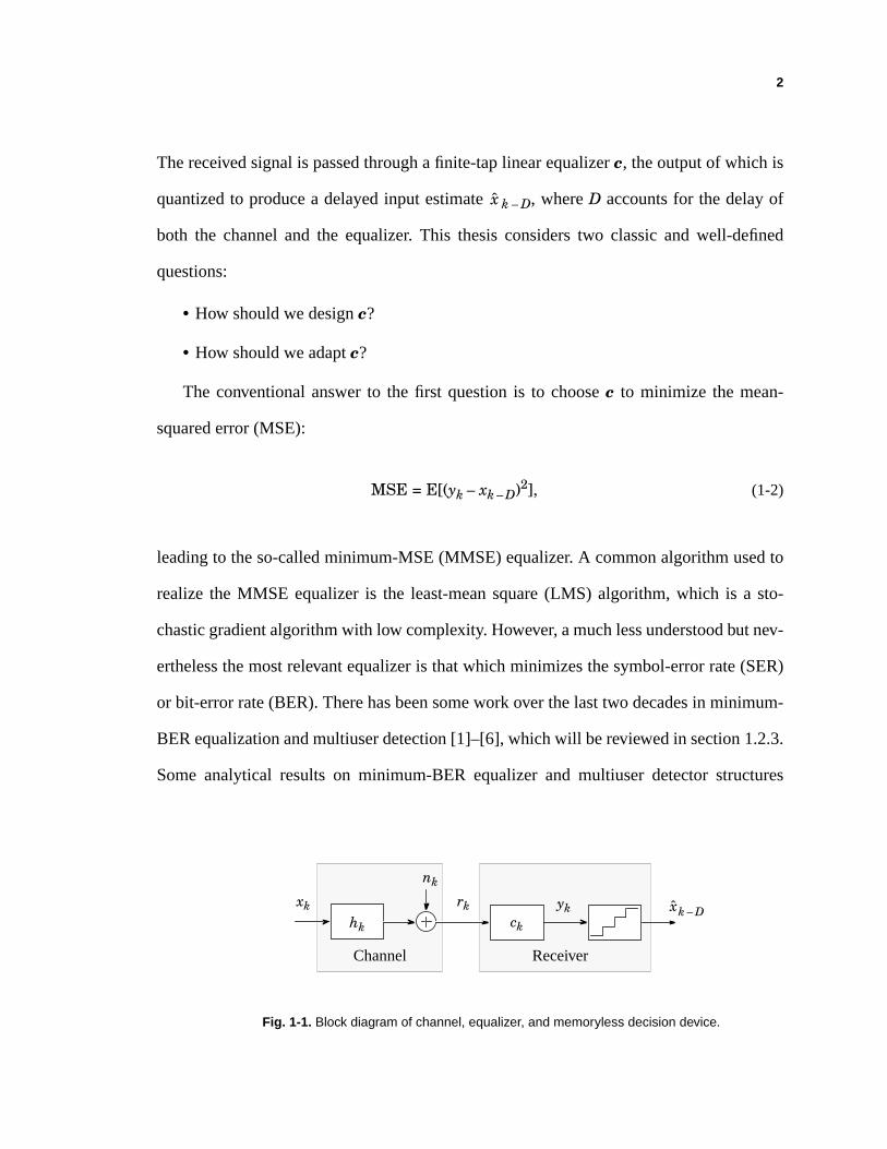
1 CHAPTER 1 I NTRODUCTION This thesis considers the design and adaptation of finite-tap equalizers for combating linear intersymbol interference (ISI) in the presence of additive white Gaussian noise, under the constraint that decisions are made on a symbol-by-symbol basis by quantizing the equalizer output. We also consider quadrature-amplitude modulation (QAM), deci- sion-feedback equalizers (DFE), and multiuser systems, but the linear ISI pulse-amplitude modulation (PAM) channel with a linear equalizer of Fig. 1-1 captures the essential fea- tures of the problem under consideration. The channel input symbols x k are drawn inde- pendently and uniformly from an L-ary PAM alphabet {±1, ±3, ... ±(L – 1)}. The channel is modeled by an impulse response h i with memory M and additive white Gaussian noise, yielding a received signal of r k = . (1-1) h i x k i – n k + i 0 = M ∑ Minimum-Error-Probability Equalization and Multiuser Detection Ph.D. Thesis, Georgia Institute of Technology, Summer 1998 Dr. Chen-Chu Yeh, [email protected]
Transcript of I NTRODUCTION - Georgia Institute of Technologyusers.ece.gatech.edu/barry/group/hall/yeh.pdfadaptive...
1
CHAPTER 1
I N T R O D U C T I O N
This thesisconsidersthedesignandadaptationof finite-tapequalizersfor combating
linear intersymbolinterference(ISI) in the presenceof additive white Gaussiannoise,
underthe constraintthat decisionsaremadeon a symbol-by-symbolbasisby quantizing
the equalizeroutput. We also considerquadrature-amplitudemodulation(QAM), deci-
sion-feedbackequalizers(DFE),andmultiusersystems,but thelinearISI pulse-amplitude
modulation(PAM) channelwith a linear equalizerof Fig. 1-1 capturesthe essentialfea-
turesof the problemunderconsideration.The channelinput symbolsxk aredrawn inde-
pendentlyanduniformly from anL-ary PAM alphabet{ ±1, ±3, ... ±(L – 1)}. Thechannel
is modeledby animpulseresponsehi with memoryM andadditive white Gaussiannoise,
yielding a received signal of
rk = . (1-1)hixk i– nk+
i 0=
M
∑
Minimum-Error-Probability Equalization and Multiuser DetectionPh.D. Thesis, Georgia Institute of Technology, Summer 1998Dr. Chen-Chu Yeh, [email protected]
2
Thereceivedsignalis passedthrougha finite-taplinearequalizerc, theoutputof which is
quantizedto producea delayedinput estimate k – D, whereD accountsfor the delayof
both the channeland the equalizer. This thesisconsiderstwo classicand well-defined
questions:
• How should we designc?
• How should we adaptc?
The conventionalanswerto the first questionis to choosec to minimize the mean-
squared error (MSE):
MSE = E[(yk – xk – D)2], (1-2)
leadingto theso-calledminimum-MSE(MMSE) equalizer. A commonalgorithmusedto
realizethe MMSE equalizeris the least-meansquare(LMS) algorithm,which is a sto-
chasticgradientalgorithmwith low complexity. However, amuchlessunderstoodbut nev-
erthelessthemostrelevantequalizeris thatwhich minimizesthesymbol-errorrate(SER)
or bit-errorrate(BER).Therehasbeensomework over thelasttwo decadesin minimum-
BERequalizationandmultiuserdetection[1]–[6], whichwill bereviewedin section1.2.3.
Someanalytical resultson minimum-BER equalizerand multiuser detectorstructures
x
xkhk
nk
rkck
yk
Fig. 1-1. Block diagram of channel, equalizer, and memoryless decision device.
Channel Receiver
xk – D
3
were derived in [1][2][4], and several adaptive minimum-BER algorithms were proposed
in [3][5][6]. However, none of the proposed adaptive algorithms guarantees convergence
to the global minimum, and the adaptive algorithms proposed in [3][5] are significantly
more complex than the LMS algorithm.
In the remainder of this chapter, we review some relevant background materials for
this thesis. In section 1.1, we review both ISI channels and multiuser interference chan-
nels. In section 1.2, we review general equalizers and multiuser detectors, their conven-
tional design criteria, and some prior work on designing equalizers and multiuser detectors
based on the error-probability criterion. In section 1.3, we outline this thesis.
1.1 INTERFERENCE CHANNELS
Interferences in communication channels are undesirable effects contributed by
sources other than noise. In this section, we discuss two types of channel interferences: (1)
intersymbol interference where adjacent data pulses distort the desired data pulse in a
linear fashion and (2) interference in multiuser systems where users other than the
intended contribute unwanted signals through an imperfect channel.
1.1.1 Intersymbol Interference
ISI characterized by (1-1) is the most commonly encountered channel impairment next
to noise. ISI typically results from time dispersion which happens when the channel fre-
quency response deviates from the ideal of constant amplitude and linear phase. In band-
width-efficient digital communication systems, the effect of each symbol transmitted over
a time-dispersive channel extends beyond the time interval used to represent that symbol.
The distortion caused by the resulting overlap of received symbols is called ISI [7]. ISI can
4
significantly close the eye of a channel, reduce noise margin and cause severe data detec-
tion errors.
1.1.2 Multiuser Interference
Multiuser interference arises whenever a receiver observes signals from multiple trans-
mitters [32]. In cellular radio-based networks using the time-division multiple-access
(TDMA) technology, frequency re-use leads to interference from other users in nearby
cells sharing the same carrier frequency, even if there is no interference among users
within the same cell. In networks using the code-division multiple-access (CDMA) tech-
nology, users are assigned distinct signature waveforms with low mutual cross-correla-
tions. When the sum of the signals modulated by multiple users is received, it is possible
to recover the information transmitted from a desired user by correlating the received
signal with a replica of the signature waveform assigned to the desired user. However, the
performance of this demodulation strategy is not satisfactory when the assigned signatures
do not have low cross-correlations for all possible relative delays. Moreover, even though
the cross-correlations between users may be low, a particularly severe multiuser interfer-
ence, referred to as near-far interference, results when powerful nearby interferers over-
whelm distant users of interest. Similar to ISI, multiuser interference reduces noise margin
and often causes data recovery impossible without some compensation means.
1.2 EQUALIZATION AND DETECTION
In the presence of linear ISI and additive white Gaussian noise, Forney [22][23]
showed that the optimum detector for linear PAM signals is a whitened-matched filter fol-
lowed by a Viterbi detector. This combined form achieves the maximum-likelihood
sequence-detector (MLSD) performance and in some cases, the matched filter bound.
5
When the channel input symbols are drawn uniformly and independently from an alphabet
set, MLSD is known to achieve the best error-probability performance of all existing
equalizers and detectors.
Although MLSD offers significant performance gains over symbol-by-symbol detec-
tors, its complexity (with the Viterbi detector) grows exponentially with the channel
memory. For channels with long ISI spans, a full-state MLSD generally serves as a mere
benchmark and is rarely used because of its large processing complexity for computing
state metrics and large memory for storing survivor path histories. Many variants of
MLSD such as channel memory truncation [24], reduced state sequence detection [26],
and fixed-delay tree search with decision-feedback [25] have been proposed to reach good
tradeoffs between complexity and performance.
Because of the often high complexity associated with MLSD, suboptimal receivers
such as symbol-by-symbol equalizers are widely used despite their inferior performance
[7]. Among all equalizers and detectors used for combating ISI, linear equalizers are the
simplest to analyze and implement. A linear equalizer combats linear ISI by de-con-
volving a linearly distorted channel with a transversal filter to yield an approximate
inverse of the channel, and a simple memoryless slicer is used to quantize the equalizer
output to reconstruct the original noiseless transmitted symbols. Unlike MLSD, equaliza-
tion enhances noise. By its design philosophy, a linear equalizer generally enhances noise
significantly on channels with severe amplitude distortion and consequently, yields poor
data recovery performance.
First proposed by Austin [27], the DFE is a significant improvement of the linear
equalizer. A DFE is a nonlinear filter that uses past decisions to cancel the interference
from prior symbols [29]–[31]. The DFE structure is beneficial for channels with severe
6
amplitude distortion. Instead of fully inverting a channel, only the forward section of a
DFE inverts the precursor ISI, while the feedback section of a DFE, being a nonlinear
filter, subtracts the post-cursor ISI. Assuming the past decisions are correct, noise
enhancement is contributed only by the forward section of the equalizer and thus noise
enhancement is reduced.
An obvious drawback of a DFE is error propagation resulting from its decision-feed-
back mechanism. A wrong decision may cause a burst of errors in the subsequent data
detection. Fortunately, the error propagation is usually not catastrophic, and this drawback
is often negligible compared to the advantage of reduced noise enhancement.
1.2.1 Conventional Design Criteria
For symbol-by-symbol equalization, zero forcing (ZF) is a well-known filter design
criterion. Lucky [7]–[10] first proposed a ZF algorithm to automatically adjust the coeffi-
cients of a linear equalizer. A ZF equalizer is simple to understand and analyze. To combat
linear ISI, a ZF linear equalizer simply eliminates ISI by forcing the overall pulse, which
is the convolution of the channel and the equalizer, to become a unit-impulse response.
Similarly, the forward section of a ZF-DFE converts the overall response to be strictly
causal, while its feedback section completely subtracts the causal ISI.
An infinite-tap ZF equalizer can completely eliminate ISI if no null exists in the
channel frequency response. By neglecting noise and concentrating solely on removing
ISI, ZF equalizers tend to enhance noise exceedingly when channels have deep nulls.
Although it has a simple adaptive algorithm, a ZF equalizer is rarely used in practice and
remains largely a textbook result and teaching tool [7].
7
Following the pioneering work by Lucky, Gersho [11] and Proakis [12] proposed
adaptive algorithms to implement MMSE equalizers. Unlike a ZF equalizer, an MMSE
equalizer maximizes the signal-to-distortion ratios by penalizing both residual ISI and
noise enhancement [7]–[18]. Instead of removing ISI completely, an MMSE equalizer
allows some residual ISI to minimize the overall distortion.
Compared with a ZF equalizer, an MMSE equalizer is much more robust in the pres-
ence of deep channel nulls and modest noise. The popularity of the MMSE equalizer is
due in part to the simple LMS algorithm proposed by Widrow and Hoff [16]. The LMS
algorithm, which is a stochastic algorithm, adjusts equalizer coefficients with a small
incremental vector in the steepest descent direction on the MSE error surface. Since the
MSE error surface is convex, the convergence of the LMS algorithm to the global min-
imum can be guaranteed when the step size is sufficiently small.
1.2.2 Low-Complexity Adaptive Equalizer Algorithms
To reduce the complexity of the LMS algorithm, several simplified variants of the
LMS algorithm have been proposed. The approximate-minimum-BER (AMBER) algo-
rithm we propose in chapter 3 is remarkably similar in form to these LMS-based algo-
rithms even though it originates from a minimum-error-probability criterion.
The sign LMS algorithm modifies the LMS algorithm by quantizing the error to ±1
according to its sign [20]. By doing so, the cost function of the sign LMS algorithm is the
mean-absolute error, E[|yk – xk – D|], instead of the mean-squared error as for the LMS
algorithm. The trade-offs for the reduced complexity are a slower convergence rate and a
larger steady-state MSE.
8
The dual-sign LMS algorithm proposed in [19] employs two different step sizes on the
sign LMS algorithm. The algorithm penalizes larger errors with a larger update step size
and therefore improves the convergence speed of the sign LMS algorithm with a small
complexity increase.
The proportional-sign algorithm proposed in [21] modifies the LMS algorithm in order
to be more robust to impulsive interference and to reduce complexity. The algorithm uses
the LMS algorithm when the equalizer output errors are small and switches to the sign
LMS algorithm when the equalizer output errors are large.
1.2.3 The Minimum-Error-Probability Criterion
Minimizing MSE should be regarded as an intermediate goal, whereas the ultimate
goal of an equalizer or a multiuser detector is to minimize the error probability. In this sec-
tion we review prior work that proposes stochastic adaptive algorithms for minimizing
error probability or analyzes the structures of the minimum-error-probability equalizers or
multiuser detectors [1]–[6].
Shamash and Yao [1] were the first to consider minimum-BER equalization. They
examined the minimum-BER DFE structure for binary signaling. Using a calculus of vari-
ation procedure, they derived the minimum-BER DFE coefficients and showed that the
forward section consists of a matched filter in tandem with a tap-delayed-line filter and the
feedback section is a tap-delayed-line filter operating to completely cancel postcursor ISI.
While the feedback section is similar to the MMSE DFE, the forward section is a solution
to a set of complicated nonlinear equations. Their work focused on a theoretical derivation
of the minimum-BER DFE structure and did not consider a numerical algorithm to com-
pute the forward filter coefficients; nor did it compare the performance of the minimum-
BER DFE to that of the MMSE DFE. Finally, an adaptive algorithm was not proposed.
9
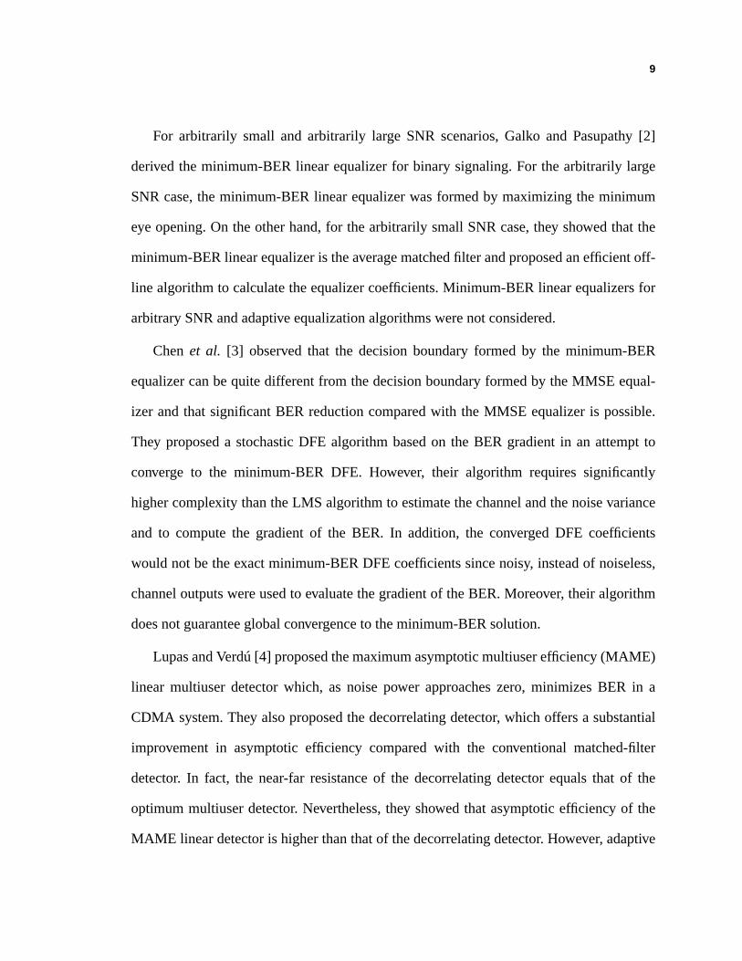
For arbitrarily small and arbitrarily large SNR scenarios,Galko and Pasupathy [2]
derived the minimum-BERlinear equalizerfor binary signaling.For the arbitrarily large
SNR case,the minimum-BERlinear equalizerwasformedby maximizingthe minimum
eye opening.On theotherhand,for thearbitrarily smallSNRcase,they showed that the
minimum-BERlinearequalizeris theaveragematchedfilter andproposedanefficientoff-
line algorithmto calculatetheequalizercoefficients.Minimum-BERlinearequalizersfor
arbitrary SNR and adaptive equalization algorithms were not considered.
Chenet al. [3] observed that the decisionboundaryformed by the minimum-BER
equalizercanbequitedifferentfrom thedecisionboundaryformedby theMMSE equal-
izer andthat significantBER reductioncomparedwith the MMSE equalizeris possible.
They proposeda stochasticDFE algorithmbasedon the BER gradientin an attemptto
converge to the minimum-BER DFE. However, their algorithm requiressignificantly
highercomplexity thantheLMS algorithmto estimatethechannelandthenoisevariance
and to computethe gradientof the BER. In addition, the converged DFE coefficients
would not betheexactminimum-BERDFE coefficientssincenoisy, insteadof noiseless,
channeloutputswereusedto evaluatethegradientof theBER.Moreover, their algorithm
does not guarantee global convergence to the minimum-BER solution.
LupasandVerdú[4] proposedthemaximumasymptoticmultiuserefficiency (MAME)
linear multiuserdetectorwhich, as noisepower approacheszero, minimizesBER in a
CDMA system.They alsoproposedthedecorrelatingdetector, which offersa substantial
improvement in asymptoticefficiency comparedwith the conventional matched-filter
detector. In fact, the near-far resistanceof the decorrelatingdetectorequalsthat of the
optimummultiuserdetector. Nevertheless,they showed that asymptoticefficiency of the
MAME lineardetectoris higherthanthatof thedecorrelatingdetector. However, adaptive
10
implementation of the MAME detector was not proposed. Moreover, the MAME linear
detector does not minimize BER when the noise power is nonzero.
Similar to the approach taken by Chen et al. [3], Mandayam and Aazhang [5] pro-
posed a BER-gradient algorithm attempting to converge to the minimum-BER multiuser
detector in a direct-sequence CDMA (DS-CDMA) system. They jointly estimated the data
of all users in the maximum-likelihood sense and used these estimates to extract an esti-
mate of the noiseless sum of all transmitted signature waveforms. This estimate was then
used to compute unbiased BER gradients. The complexity of the algorithm is exceedingly
high, especially when the number of users is large. In addition, the algorithm can converge
to a non-global local minimum.
Based on a stochastic approximation method for finding the extrema of a regression
function, Psaromiligkos et al. [6] proposed a simple linear DS-CDMA detector algorithm
that does not involve the BER gradient. They derived a stochastic quantity whose expecta-
tion is BER and applied a stochastic recursion to minimize it. However, the algorithm can
also converge to a nonglobal local BER minimum detector.
Although some important issues on minimum-error-probability equalizers and mul-
tiuser detectors were addressed by the above-mentioned prior works, a unified theory for
minimum-error-probability equalization and multiuser detection is still not in place. In
addition, the performance gap between the MMSE and minimum-error-probability equal-
izers and multiuser detectors has not been thoroughly investigated. Also, none of the
above-mentioned prior works considered non-binary modulation. Most importantly, a
simple, robust, and globally convergent stochastic algorithm had not yet been proposed to
be comparable to its MMSE counterpart, the LMS algorithm.
11
1.3 THESIS OUTLINE
This thesis aims to design and adapt finite-tap equalizers and linear multiuser detectors
to minimize error probability in the presence of intersymbol interference, multiuser inter-
ference, and Gaussian noise.
In chapter 2, we present system models and concepts which are essential in under-
standing the minimum-error-probability equalizers and multiuser detectors. We first derive
a fixed-point relationship to characterize the minimum-error-probability linear equalizers.
We then propose a numerical algorithm, called the exact minimum-symbol-error-rate
(EMSER) algorithm, to determine the linear equalizer coefficients of Fig. 1-1 that mini-
mize error probability. We study the convergence properties of the EMSER algorithm and
propose a sufficiency condition test for verifying its convergence to the global error-prob-
ability minimum. We also extend the EMSER algorithm to QAM and DFE.
In chapter 3, we use a function approximation to alter the EMSER algorithm such that
a very simple stochastic algorithm becomes available. We form a stochastic algorithm by
incorporating an error indicator function whose expectation is related to the error proba-
bility. The proposed algorithm has low complexity and is intuitively sound, but neverthe-
less has some serious shortcomings. To overcome these shortcomings, an adaptation
threshold is added to the stochastic algorithm to yield a modified algorithm, called the
approximate minimum-bit-error-rate (AMBER) algorithm. Compared with the original
stochastic algorithm, the AMBER algorithm has a faster convergence speed and is able to
operate in a decision-directed mode. We compare the steady-state error probability of the
AMBER equalizer with that of the MMSE equalizer. In addition, we device a crude char-
acterize procedure to predict the ISI channels for which the AMBER and EMSER equal-
izers can outperform MMSE equalizers.
12
In chapter 4, we study the convergence properties of the AMBER algorithm and pro-
pose a variant to improve its convergence speed. We first take the expectation of the
AMBER algorithm to derive its ensemble average. By obtaining its ensemble average, we
analyze the global convergence properties of the AMBER algorithm. We then propose
multi-step AMBER algorithms to further increase the convergence speed.
In chapter 5, we extend the results on the EMSER and AMBER equalizers to mul-
tiuser applications. Multiuser interference is similar in many respects to the ISI phenom-
enon in a single-user environment. We study the performance of the AMBER algorithm on
multiuser channels without memory.
In chapter 6, we conclude our study and propose some interesting topics for future
research.
13
CHAPTER 2
M I N I M U M - S E RE Q U A L I Z A T I O N
2.1 INTRODUCTION
As mentioned in chapter 1, an MMSE equalizer is generally different from the min-
imum-error-probability equalizer. Although most finite-tap linear equalizers are designed
to minimize an MSE performance metric, the equalizer that directly minimizes symbol-
error-rate (SER) may significantly outperform the MMSE equalizer. In this chapter, we
first derive the minimum-SER linear equalizer for PAM. We study the properties of the
minimum-SER equalizer by exploring its geometric interpretation and compare its SER
performance to the MMSE equalizer. We also devise a numerical algorithm, called the
exact minimum-symbol-error-rate (EMSER) algorithm, to compute the equalizer coeffi-
cients. We study the convergence properties of the EMSER algorithm. Finally we extend
the derivation of the minimum-SER linear equalizer for PAM to QAM and DFE.

14
In section 2.2, we present the system model of the ISI channel and the linear equalizer,
and we explain the concepts of signal vectors and signal cones, which are essential tools in
deriving and understanding the minimum-SER equalizer and its adaptive algorithm. In
section 2.3, we derive a fixed-point relationship to characterize the minimum-SER equal-
izer, and we compare the minimum-SER equalizer with the MMSE equalizer when the
number of equalizer coefficients approaches infinity. In section 2.4, based on the fixed-
point relationship, we propose a numerical method to compute the minimum-SER equal-
izer coefficients. We then study the convergence properties of the numerical method and
state a sufficiency condition for testing convergence of the numerical method to the global
SER minimum. In section 2.5, we extend the minimum-SER results on PAM to QAM. In
section 2.6, we derive the minimum-SER decision-feedback equalizer.
2.2 MODELS FOR CHANNEL AND EQUALIZER
2.2.1 System Definition
Consider the real-valued linear discrete-time channel depicted in Fig. 2-1, where the
channel input symbols xk are drawn independently and uniformly from the L-ary PAM
alphabet {±1, ±3, …, ± (L – 1)}, hk is the FIR channel impulse response nonzero for k = 0
… M only, and nk is white Gaussian noise with power spectral density σ2. The channel
output rk is
xk
hk
nkrk
ck
yk k–Dx
Fig. 2-1. Block diagram of channel, equalizer, and memoryless decision device.
Channel Receiver
15
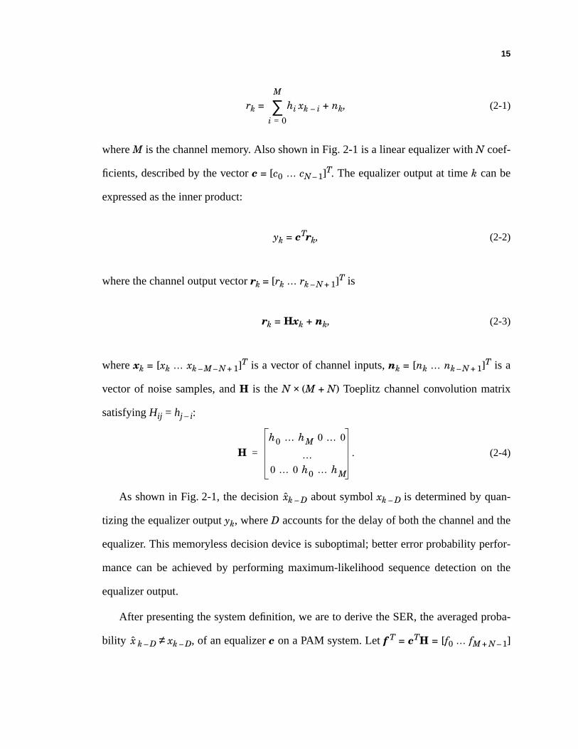
rk = hi xk – i + nk, (2-1)
where M is the channel memory. Also shown in Fig. 2-1 is a linear equalizer with N coef-
ficients, described by the vector c = [c0 … cN – 1]T. The equalizer output at time k can be
expressed as the inner product:
yk = cTrk, (2-2)
where the channel output vector rk = [rk … rk – N + 1]T is
rk = Hxk + nk, (2-3)
where xk = [xk … xk – M – N + 1]T is a vector of channel inputs, nk = [nk … nk – N + 1]T is a
vector of noise samples, and H is the N × (M + N) Toeplitz channel convolution matrix
satisfying Hij = hj – i:
. (2-4)
As shown in Fig. 2-1, the decision k – D about symbol xk – D is determined by quan-
tizing the equalizer output yk, where D accounts for the delay of both the channel and the
equalizer. This memoryless decision device is suboptimal; better error probability perfor-
mance can be achieved by performing maximum-likelihood sequence detection on the
equalizer output.
After presenting the system definition, we are to derive the SER, the averaged proba-
bility k – D ≠ xk – D, of an equalizer c on a PAM system. Let f T = cTH = [f0 … fM + N – 1]
i 0=
M
∑
Hh0 … hM 0 … 0
…0 … 0 h0 … hM
=
x
x
16
denotethe overall impulseresponse,representingthe cascadeof the channelhk andthe
equalizerck. The noiseless equalizer output is
cTHxk = f Txk
= fD xk – D + fixk – i, (2-5)
wherethe first term fD xk – D representsthe desiredsignallevel, whereasthe secondterm
represents residual ISI. The noisy equalizer output of (2-2) is also expressed as:
yk = fD xk – D + fixk – i + cTnk. (2-6)
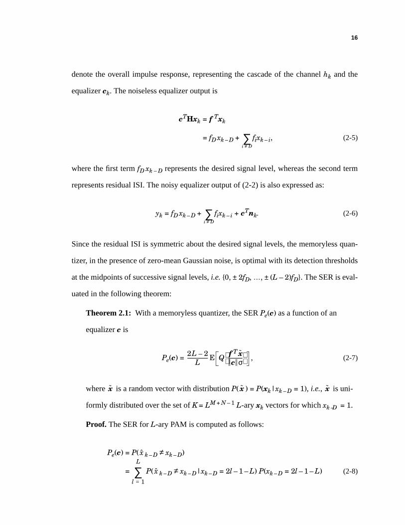
SincetheresidualISI is symmetricaboutthedesiredsignallevels,thememorylessquan-
tizer, in thepresenceof zero-meanGaussiannoise,is optimalwith its detectionthresholds
at themidpointsof successivesignallevels,i.e. {0, ± 2fD, …, ± (L – 2)fD}. TheSERis eval-
uated in the following theorem:
Theorem 2.1: With a memoryless quantizer, the SERPe(c) as a function of an
equalizerc is
Pe(c) = E , (2-7)
where is a randomvectorwith distribution P( ) = P(xk|xk – D = 1), i.e., is uni-
formly distributedover thesetof K = LM + N – 1 L-aryxk vectorsfor which xk –D = 1.
Proof. The SER forL-ary PAM is computed as follows:
Pe(c) = P( k – D ≠ xk – D)
= P( k – D ≠ xk – D|xk – D = 2l – 1 – L) P(xk – D = 2l – 1 – L) (2-8)
i D≠∑
i D≠∑
2L 2–L
----------------- Q f T xc σ
-----------
x x x
x
l 1=
L
∑ x
17
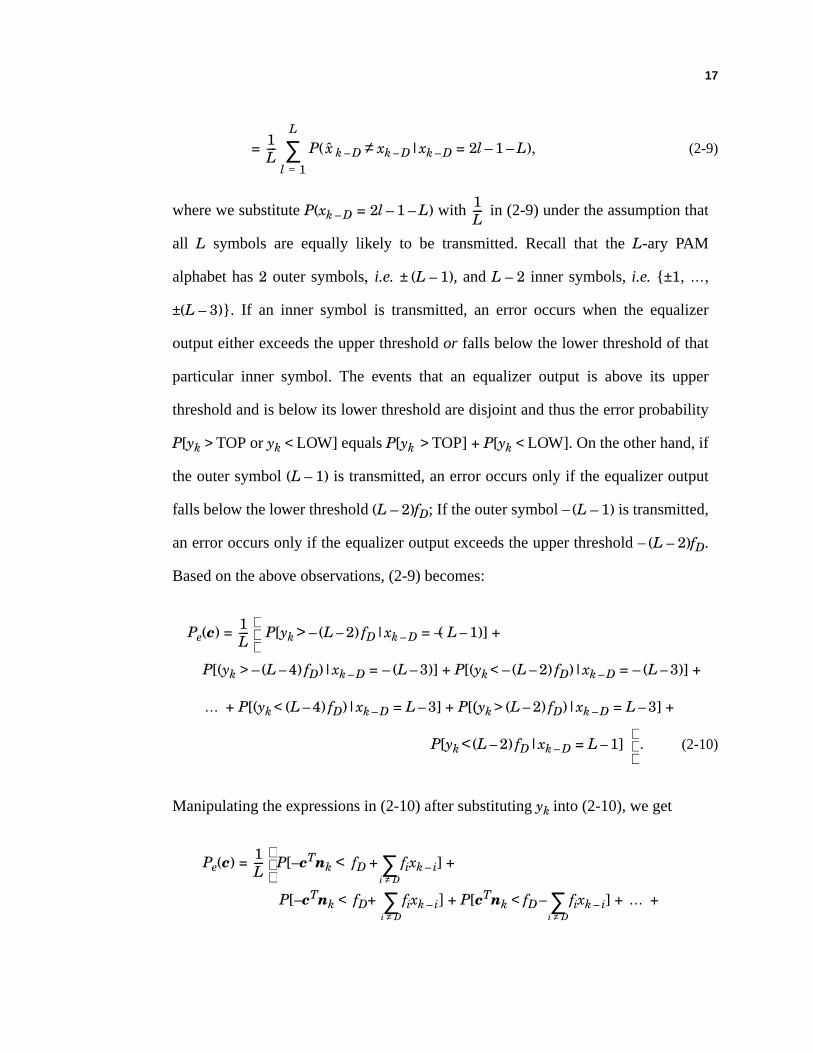
= P( k – D ≠ xk – D|xk – D = 2l – 1 – L), (2-9)
where we substitute P(xk – D = 2l – 1 – L) with in (2-9) under the assumption that
all L symbols are equally likely to be transmitted. Recall that the L-ary PAM
alphabet has 2 outer symbols, i.e. ± (L – 1), and L – 2 inner symbols, i.e. {±1, …,
±(L – 3)}. If an inner symbol is transmitted, an error occurs when the equalizer
output either exceeds the upper threshold or falls below the lower threshold of that
particular inner symbol. The events that an equalizer output is above its upper
threshold and is below its lower threshold are disjoint and thus the error probability
P[yk > TOP or yk < LOW] equals P[yk > TOP] + P[yk < LOW]. On the other hand, if
the outer symbol (L – 1) is transmitted, an error occurs only if the equalizer output
falls below the lower threshold (L – 2)fD; If the outer symbol – (L – 1) is transmitted,
an error occurs only if the equalizer output exceeds the upper threshold – (L – 2)fD.
Based on the above observations, (2-9) becomes:
Pe(c) = P[yk > – (L – 2) fD|xk – D = –( L – 1)] +
P[(yk > – (L – 4) fD)|xk – D = – (L – 3)] + P[(yk < – (L – 2) fD)|xk – D = – (L – 3)] +
+ P[(yk < (L – 4) fD)|xk – D = L – 3] + P[(yk > (L – 2) fD)|xk – D = L – 3] +
P[yk < (L – 2) fD|xk – D = L – 1] . (2-10)
Manipulating the expressions in (2-10) after substituting yk into (2-10), we get
Pe(c) = P[– cTnk < fD + fixk – i] +
P[– cTnk < fD+ fixk – i] + P[cTnk < fD – fixk – i] + +
1L----
l 1=
L
∑ x
1L----
1L----
…
1L----
i D≠∑
i D≠∑
i D≠∑ …
18
P[cTnk < fD – fixk – i] + P[– cTnk < fD + fixk – i] +
P[cTnk < fD – fixk – i] . (2-11)
Note that in (2-11) we have removed the condition on the value of xk – D from all
expressions in (2-10) since they do not depend on the condition any more. In addi-
tion, the random variables – cTnk and – fixk – i respectively have the same proba-
bility distributions as cTnk and fixk – i and we can exchange them to simplify (2-
11) as follows:
Pe(c) = P[cTnk < fD + fixk – i] +
P[cTnk < fD+ fixk – i] + P[cTnk < fD + fixk – i] + +
P[cTnk < fD + fixk – i] + P[– cTnk < fD + fixk – i] +
P[cTnk < fD + fixk – i]
= P[cTnk < fD + fixk – i]
= P[cTnk < f Tx(i)]
=
= E , (2-12)
where Q is the Gaussian error function, where x(1), x(2), …, x(K) are any ordering of
the K distinct vectors, and where the expectation is over the K equally likely
vectors. Q.E.D.
Therefore, minimizing SER of an L-PAM system is equivalent to minimizing the term
E . In the case of a 2-PAM system, the factor in (2-12) reduces to unity.
i D≠∑
i D≠∑
i D≠∑
i D≠∑
i D≠∑
1L----
i D≠∑
i D≠∑
i D≠∑ …
i D≠∑
i D≠∑
i D≠∑
2L 2–L
-----------------i D≠∑
2L 2–L
----------------- 1K-----
K
i 1=∑2L 2–
L----------------- 1
K-----
K
i 1=∑ Q f T x i( )
c σ-----------------
2L 2–L
----------------- Q f T xc σ
-----------
x x
Q f T xc σ
----------- 2L 2–
L-----------------
19
Even though it is most relevant to minimize the error probability of (2-12), by far the
most popular equalization strategy is the MMSE design. With the MMSE strategy, the
equalizer c is chosen as the unique vector minimizing MSE = E[(yk – xk – D)2], namely:
cMMSE = (HHT + σ2I)– 1hD+1, (2-13)
where hD + 1 is the (D + 1)-st column of H. This equalizer is often realized using a sto-
chastic gradient search known as the least-mean square (LMS) algorithm [7]:
ck + 1 = ck – µ(yk – x k – D)rk, (2-14)
where µ is a small positive step size. When training data is unavailable, the equalizer can
operate in a decision-directed mode, whereby the decision k – D is used in place of xk – D.
Instead of minimizing MSE, our goal is to minimize SER (2-12). For a binary sig-
naling channel it is obvious that BER is the same as SER. However, for a non-binary PAM
channel, the exact relationship between SER and BER is not trivial. With the Gray code
mapping of bits, the relationship is well approximated by [13]:
BER ≅ SER. (2-15)
Therefore, if an equalizer minimizes SER, it approximately minimizes BER.
2.2.2 Signal Vectors and Signal Cones
In this section, we introduce the signal vectors and the signal cone, two useful geo-
metric tools that will be used extensively throughout the thesis to derive and understand
minimum-SER equalizers.
x
1
2Llog
---------------
20
We now establish the relationship between error probability and signal vectors.
Observe that the error probability of (2-12) can also be expressed as
Pe(c) = E , (2-16)
where the expectation is over the K equally likely L-ary vectors. We define the signal
vectors by
s(i) = Hx(i), i = 1 … K. (2-17)
From (2-3) we see that these s(i) vectors represent the K possible noiseless channel output
vectors given that the desired symbol is xk–D = 1. With this definition, (2-16) can be
expressed as
Pe(c) = . (2-18)
Observe that the error probability is proportional to the average of the K Q function terms,
the argument of each being proportional to the inner product between the equalizer and a
signal vector.
In this thesis we will often assume that the channel is equalizable:
Definition 1. A channel is said to be equalizable by an N-tap equalizer with delay
D if and only if there exists an equalizer c having a positive inner product with all
{s(i)} signal vectors.
A positive inner product with all {s(i)} vectors implies that the noiseless equalizer output
is always positive when a one was transmitted (xk–D = 1); thus, a channel is equalizable if
2L 2–L
----------------- Q cTH xc σ
----------------
x
2L 2–KL
-----------------
i 1=
K
∑ Q cTs i( )
c σ----------------
21
and only if its noiselesseye diagramcan be opened.In terms of the { s(i)} vectors,a
channelis equalizableif andonly if thereexists a hyperplanepassingthroughthe origin
such that all {s(i)} vectors are strictly on one side of the hyperplane.
Givena setof signalvectors{ s(i)} thatcanbe locatedstrictly on onesideof a hyper-
planepassingthroughthe origin, we definethe signal cone asthe spanof thesevectors
with non-negative coefficients:
Definition 2. The signal cone of an equalizable channel is the set:
S = { Σi ais(i) : ai ≥ 0}.
Observe thatif thechannelis equalizable,thereexistsat leastone“axis” vectorwithin the
signalconesuchthatall elementsof thesignalconeform anangleof strictly lessthan90˚
with respectto theaxisvector. We remarkthatno suchaxisvectorexists if thechannelis
not equalizable, because the set {Σi ais(i) : ai ≥ 0} is a linear subspace of N in this case.
With the signalvectorsandthe signalconedefined,we arenow equippedto charac-
terize the minimum-SER equalizer.
2.3 CHARACTERIZA TION OF THE MINIMUM-SER EQ UALIZER
2.3.1 Fixed-Point Relationship
Let cEMSER denoteanequalizerthatachievesexactminimum-SER(EMSER)perfor-
mance,minimizing (2-16).Observe thatbecause(2-16)dependsonly on thedirectionof
theequalizer, cEMSER is not unique:if c minimizesSER,thensodoesac for any positive
constanta. Unlike the coefficient vectorcMMSE (2-13) that minimizesMSE, thereis no
closed-formexpressionfor cEMSER. However, by settingto zero the gradientof (2-16)
with respect toc:
R
22
∇cPe(c) = E = 0, (2-19)
we find that cEMSER, which is a global minimum solution to (2-16), must satisfy
|| c ||2f(c) = cTf(c)c, (2-20)
where we have introduced the function f : N → N, defined by
f(c) = E . (2-21)
The expectation in (2-21) is with respect to the random vector s over the K equally likely
s(i) vectors of (2-17). Thus, f(c) can be expressed as a weighted sum of s(i) vectors:
f(c) = s(1) + s(2) + … + s(K) , (2-22)
where αi = cTs(i) ⁄ (||c|| σ) is a normalized inner product of s(i) with c.
The function f(c) plays an important role in our analysis and has a useful geometric
interpretation. Observe first that, because the exponential coefficients in (2-22) are all pos-
itive, f(c) is inside the signal cone. Because exp( ⋅ ) is an exponentially decreasing func-
tion, (2-22) suggests that f(c) is dictated by only those s(i) vectors whose inner products
with c are relatively small. Because the {s(i)} vectors represent the K possible noiseless
channel output vectors given that a one was transmitted (i.e. xk–D = 1), the inner product
s(i) with c is a noiseless equalizer output given that a one is transmitted. It follows that a
small inner product is equivalent to a nearly closed eye diagram. Therefore, f(c) will be
very nearly a linear combination of the few s(i) vectors for which the eye diagram is most
12πσ
--------------- cTs( )2–
2 c 2σ2---------------------
c 2s cTsc–
c 3-------------------------------exp
R R
cTs( )2–
2 c 2σ2---------------------
sexp
1K-----
eα1
2– 2⁄e
α22– 2⁄
eαK
2– 2⁄
23
closed. For example, if one particular s(i) vector closes the eye significantly more than any
other s(i) vector, then f(c) will be approximately proportional to that s(i) vector.
Returning to (2-20) and the problem of finding the EMSER equalizer, we see that one
possible solution of (2-20) is f(c) = 0. We now show that f(c) = 0 is impossible when the
channel is equalizable. Recall that, if the channel is equalizable, then there exists a hyper-
plane passing through the origin such that all of the {s(1), …, s(L)} vectors are strictly on
one side of the hyperplane. Thus, any linear combination of s(i) with strictly positive coef-
ficients cannot be zero. Furthermore, (2-22) indicates that f(c) is a linear combination of
{s(i)} vectors with strictly positive coefficients. Thus, we conclude that f(c) = 0 is impos-
sible when the channel is equalizable.
Since f(c) = 0 is impossible when the channel is equalizable, the only remaining solu-
tion to (2-20) is the following fixed-point relationship:
c = af(c), (2-23)
for some constant a. Choosing a = 0 results in Pe = (L – 1) ⁄ L, which is clearly not the
minimum error probability of an equalizable channel. The sign of a does not uniquely
determine whether c = af(c) is a local minimum or local maximum; however, in order for
c = af(c) to be a global minimum, a must be positive:
Lemma 2-1: If c minimizes error probability of an equalizable channel, then
c = af(c) with a > 0. (2-24)
Proof. By contradiction: Suppose that c = af(c) minimizes error probability with
a < 0. Then c is outside the signal cone generated by {s(i)}. Let P denote any hyper-
24
plane,containingtheorigin, thatseparatesc from thesignalcone.Let c´ denotethe
reflectionof c aboutP suchthatc´ andthesignalconeareon thesamesideof P. It
is easyto show thatcomparedwith c, c´ hasa largerinnerproductwith all s(i) vec-
tors.From(2-18)it follows thattheerrorprobabilityfor c´ is smallerthantheerror
probability for c, which contradictsthe assumptionthat c minimizeserror proba-
bility. Q.E.D.
Unfortunately, thefixed-pointrelationshipof (2-24) is not sufficient in describingthe
EMSERequalizer;it simply statesa necessaryconditionthat theEMSERequalizermust
satisfy. The existenceof at leastoneunit-lengthvector = satisfying(2-23) canbe
intuitively explained:Thehypersphereof all unit-lengthvectors is closed,continuous,
andbounded.Eachpoint on the hypersphereis mappedto a real valuevia the differen-
tiableandboundederrorprobability functionof (2-18)andformsanotherclosed,contin-
uous,and boundedsurface.Becausethe resultantsurface is everywheredifferentiable,
closed,andbounded,it hasat leastonelocal minimum.In general,thereexist morethan
one local minima, as illustrated in the following example.
Example 2-1: Consider binary signaling xk ∈{±1} with a transfer function
H(z) = –0.9 + z–1 and a two-tap linear equalizer (N = 2) and delay D = 1. In
Fig. 2-2 we presenta polar plot of BER (for BPSK, the error probability equals
BER)versusθ, where = [cosθ, sinθ]T. Superimposedon thisplot aretheK = 4
signalvectors{ s(1), …, s(4)} , depictedby solid lines.Also superimposedarethree
unit-lengthequalizervectors(depictedby dashedlines):theEMSERequalizerwith
an angle of θ = –7.01 ˚, the MMSE equalizer with θ = –36.21 ˚, and a local
minimumequalizer( LOCAL) with θ = 35.63˚. (A fourthequalizerwith anangleof
θ = –5.84 ˚ is also depictedfor future reference:it is the approximateminimum-
c cc-------
c
cc-------
c

25
BER (AMBER) equalizer defined by Theorem 3.1 of section 3.2.) The shaded
region denotes the signal cone. Although both EMSER and LOCAL satisfy (2-23)
with a > 0, the local-minimum equalizer LOCAL does not minimize BER, and it
does not open the eye diagram. These equalizers assume SNR = 20 dB.
While Lemma 2-1 provides a necessary condition for the EMSER equalizer, namely
c = af(c) with a > 0, the previous example illustrates that this fixed-point condition is not
Fig. 2-2. A polar plot of BER versus θ for Example 2-1. Superimposed are thesignals vectors (scaled by a factor of 0.5), and four equalizer vectors (dashedlines).
s(1)
s(4)
s(3)s(2)
BER
EMSER
MMSEc
c
LOCALc
AMBERc
c c
c
26
sufficient; both cEMSER andcLOCAL satisfyc = af(c) with a > 0, but only cEMSER mini-
mizes error probability.
As anaside,aninterestingexamplecanbeconstructedto show thattheEMSERequal-
izer maynot opentheeye evenwhenopeningtheeye is possible(i.e. whenthechannelis
equalizable).The following exampleis somewhat counter-intuitive andis a resultof the
highly irregular shape of the error probability surface.
Example 2-2: ConsiderthebinarysignalingchannelH(z) = 1 – z–1 + 1.2 z–2 with a
two-tapequalizer, D = 3, andSNR= 10 dB. Although the channelis equalizable,
neither the EMSER equalizer nor the MMSE equalizer opens the eye.
2.3.2 The MMSE Equalizer vs. the EMSER Equalizer
Wenow comparetheMMSE andtheEMSERequalizers.With afinite numberof taps,
theMMSE andtheEMSERequalizersareclearlytwo differentequalizers,asillustratedin
Example2-1. We furtheremphasizethedifferencesbetweenthetwo equalizersby evalu-
ating their error-probability performanceand by plotting their eye diagramsin the fol-
lowing examples.
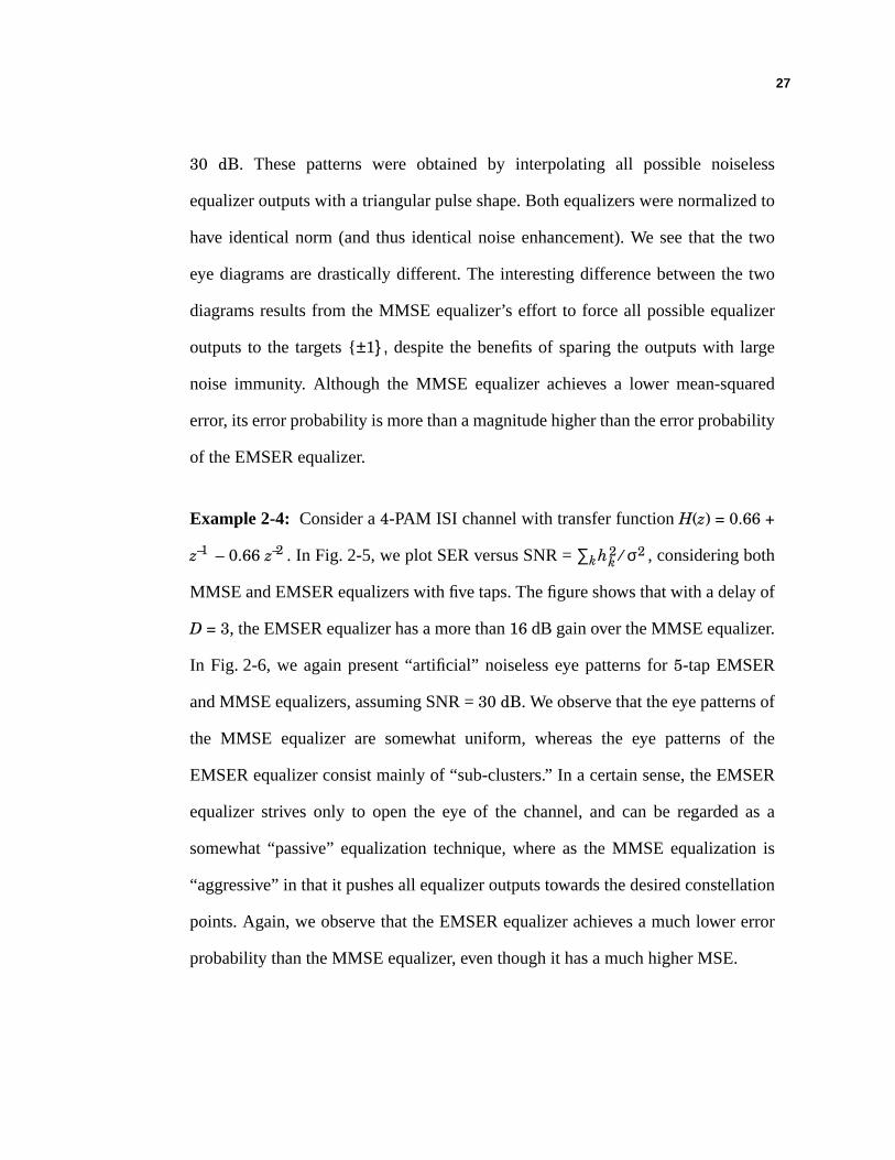
Example 2-3: Consider a binary-signaling channel with transfer function
H(z) = 1.2 + 1.1z–1 – 0.2z–2 . In Fig. 2-3, weplot BERversusSNR= ∑k , for
both the MMSE andEMSERequalizerwith threeandfive taps.The figure shows
thatwith threeequalizertapsanda delayof D = 2. D is chosento minimizeMSE.
TheEMSERequalizerhasamorethan6.5dB gainover theMMSE equalizer. With
5 equalizertapsanda delayof D = 4, theEMSERequalizerhasa nearly2 dB gain
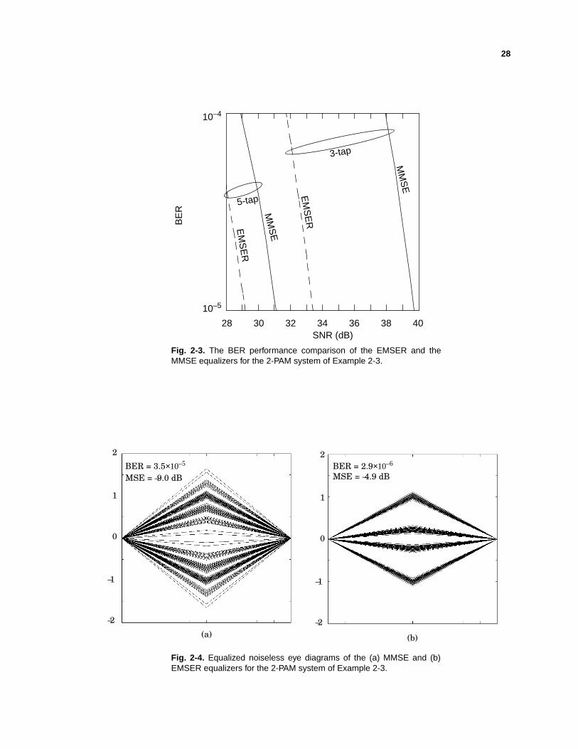
over theMMSE equalizer. In Fig. 2-4, for thesamechannel,we present“artificial”
noiselesseye patternsfor 5-tap EMSERandMMSE equalizers,assumingSNR =
hk2 σ2⁄
27
30 dB. These patterns were obtained by interpolating all possible noiseless
equalizeroutputswith a triangularpulseshape.Bothequalizerswerenormalizedto
have identicalnorm (and thus identicalnoiseenhancement).We seethat the two
eye diagramsaredrasticallydifferent.The interestingdifferencebetweenthe two
diagramsresultsfrom the MMSE equalizer’s effort to force all possibleequalizer
outputsto the targets{ ±1}, despitethe benefitsof sparingthe outputswith large
noise immunity. Although the MMSE equalizerachieves a lower mean-squared
error, its errorprobabilityis morethanamagnitudehigherthantheerrorprobability
of the EMSER equalizer.
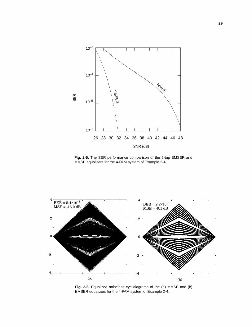
Example 2-4: Considera 4-PAM ISI channelwith transferfunctionH(z) = 0.66 +
z–1 – 0.66 z–2 . In Fig. 2-5, we plot SERversusSNR= ∑k , consideringboth
MMSE andEMSERequalizerswith five taps.Thefigureshows thatwith adelayof
D = 3, theEMSERequalizerhasamorethan16 dB gainover theMMSE equalizer.
In Fig. 2-6, we again present“artificial” noiselesseye patternsfor 5-tap EMSER
andMMSE equalizers,assumingSNR= 30 dB. Weobserve thattheeyepatternsof
the MMSE equalizerare somewhat uniform, whereasthe eye patternsof the
EMSERequalizerconsistmainly of “sub-clusters.” In a certainsense,theEMSER
equalizerstrives only to openthe eye of the channel,and can be regardedas a
somewhat “passive” equalizationtechnique,whereas the MMSE equalizationis
“aggressive” in thatit pushesall equalizeroutputstowardsthedesiredconstellation
points.Again, we observe that theEMSERequalizerachievesa muchlower error
probability than the MMSE equalizer, even though it has a much higher MSE.
hk2 σ2⁄
28
Fig. 2-3. The BER performance comparison of the EMSER and theMMSE equalizers for the 2-PAM system of Example 2-3.
28 30 32 34 36 38 40
10–5
10–4
MM
SE
EM
SE
R
MM
SE
EM
SE
RSNR (dB)
BE
R
3-tap
5-tap
Fig. 2-4. Equalized noiseless eye diagrams of the (a) MMSE and (b)EMSER equalizers for the 2-PAM system of Example 2-3.
–2
–1
0
1
2
–2
–1
0
1
2
(a) (b)
BER = 3.5×10⁻⁵ BER = 2.9×10⁻⁶
MSE = –4.9 dBMSE = –9.0 dB
29
MMSE
SNR (dB)
SE
R
EM
SE
R
10–5
10–4
10–3
Fig. 2-5. The SER performance comparison of the 5-tap EMSER andMMSE equalizers for the 4-PAM system of Example 2-4.
26 28 30 32 34 36 38 40 42 44 46 48
10–6
Fig. 2-6. Equalized noiseless eye diagrams of the (a) MMSE and (b)EMSER equalizers for the 4-PAM system of Example 2-4.
BER = 5.4×10⁻⁴
MSE = –16.2 dB
(a) (b)
–4
–2
0
2
4
–4
–2
0
2
4BER = 2.2×10⁻⁵
MSE = –9.1 dB
30
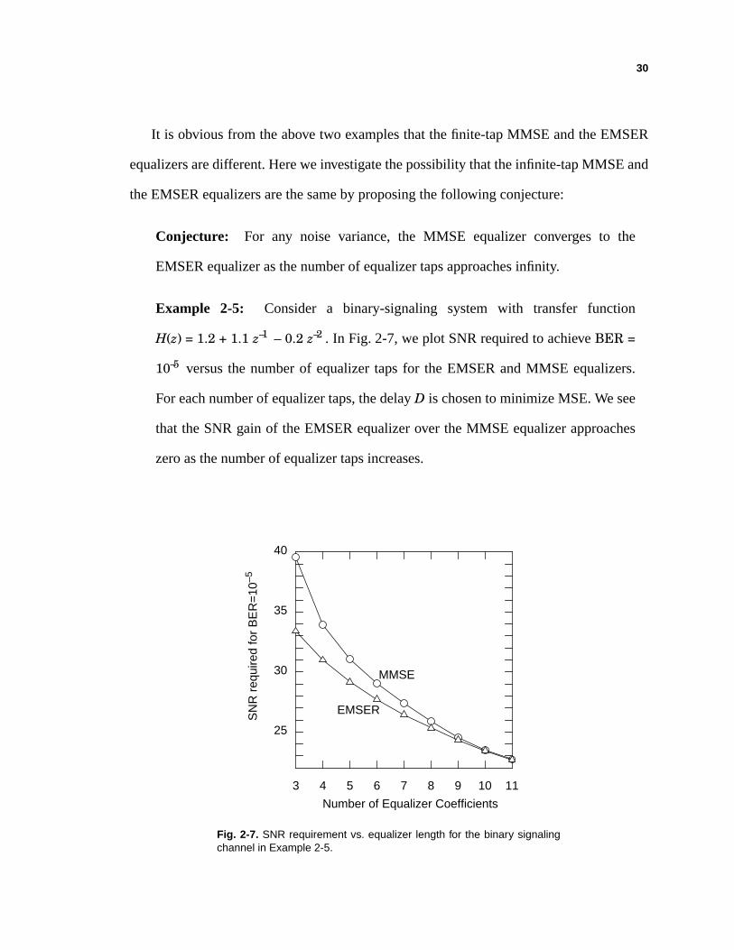
It is obvious from the above two examples that the finite-tap MMSE and the EMSER
equalizers are different. Here we investigate the possibility that the infinite-tap MMSE and
the EMSER equalizers are the same by proposing the following conjecture:
Conjecture: For any noise variance, the MMSE equalizer converges to the
EMSER equalizer as the number of equalizer taps approaches infinity.
Example 2-5: Consider a binary-signaling system with transfer function
H(z) = 1.2 + 1.1 z–1 – 0.2 z–2 . In Fig. 2-7, we plot SNR required to achieve BER =
10–5 versus the number of equalizer taps for the EMSER and MMSE equalizers.
For each number of equalizer taps, the delay D is chosen to minimize MSE. We see
that the SNR gain of the EMSER equalizer over the MMSE equalizer approaches
zero as the number of equalizer taps increases.
Fig. 2-7. SNR requirement vs. equalizer length for the binary signalingchannel in Example 2-5.
3 4 5 6 7 8 9 10 11
25
30
35
40
Number of Equalizer Coefficients
MMSE
EMSERSN
R r
equi
red
for
BE
R=
10–5
31
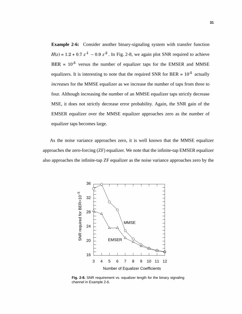
Example 2-6: Consider another binary-signaling system with transfer function
H(z) = 1.2 + 0.7 z–1 – 0.9 z–2 . In Fig. 2-8, we again plot SNR required to achieve
BER = 10–5 versus the number of equalizer taps for the EMSER and MMSE
equalizers. It is interesting to note that the required SNR for BER = 10–5 actually
increases for the MMSE equalizer as we increase the number of taps from three to
four. Although increasing the number of an MMSE equalizer taps strictly decrease
MSE, it does not strictly decrease error probability. Again, the SNR gain of the
EMSER equalizer over the MMSE equalizer approaches zero as the number of
equalizer taps becomes large.
As the noise variance approaches zero, it is well known that the MMSE equalizer
approaches the zero-forcing (ZF) equalizer. We note that the infinite-tap EMSER equalizer
also approaches the infinite-tap ZF equalizer as the noise variance approaches zero by the
Fig. 2-8. SNR requirement vs. equalizer length for the binary signalingchannel in Example 2-6.
3 4 5 6 7 8 9 10 11 12
16
20
24
28
32
36
Number of Equalizer Coefficients
MMSE
EMSERSN
R r
equi
red
for
BE
R=
10–5
32
following reasoning: If an equalizer c has an infinite number of taps, it can invert a FIR
channel completely, i.e. there exists a zero-forcing vector c such that the inner products
between c and all signal vectors s(i) are unity. If the infinite-tap minimum-SER equalizer
does not equal the zero-forcing vector, some inner products cTs(i) are smaller than others
and thus, as the noise variance approaches zero, the overall SER is solely dictated by the Q
term associated with the smallest inner product. A lower SER can be obtained by adjusting
c to increase the smallest inner product until it equals the largest inner product, or when
the equalizer becomes the ZF equalizer.
It is not clear whether the infinite-tap MMSE equalizer equals the infinite-tap EMBER
equalizer with an arbitrary noise variance. An interesting observation is that the MMSE
linear equalizer with a large number of taps tends to make the residual ISI Gaussian-like,
although this Gaussian-like distribution is bounded. A true Gaussian random variable is
unbounded.
2.4 A NUMERICAL METHOD
In section 2.3, we have gained some good understanding of the EMSER equalizer by
characterizing it with a fixed-point relationship. We now proceed to devise a numerical
algorithm to actually compute the EMSER equalizer coefficients.
2.4.1 The Deterministic EMSER Algorithm
Example 2-1 in the previous section illustrates that the error probability function may
not be convex. Nevertheless, a gradient algorithm may still be used to search for a local
minimum. In particular, using the gradient (2-19) of the SER (2-16), we may form a gra-
dient algorithm:

33
ck+1 = ck – µ1 Pe
= 1 – µckTf(ck) ⁄ ||ck ||2 ck + µf(ck)
= 1 – µckTf(ck) ⁄ ||ck ||2 ck + f(ck) , (2-25)
wherethefunctionf (⋅) is definedby (2-21).Recallthatthenormof c hasno impacton Pe,
andobserve that thefirst bracketedfactorin (2-25) representsanadjustmentof thenorm
of ck+1. Eliminating this factorleadsto the following recursion,which we refer to asthe
EMSER algorithm:
ck+1 = ck + µf(ck). (2-26)
The transformationfrom (2-25) to (2-26) affects the convergencerate, the steady-state
norm ||c∞ ||, andpossiblythe steady-statedirectionc∞ ⁄ ||c∞ ||, so it is no longerappro-
priateto call (2-26)agradientsearchalgorithm.Theupdateequation(2-26)canbeviewed
as an iterative system designed to recover the solution to the fixed-point equation (2-24).
2.4.2 Convergence
Although the EMSERalgorithmcannotin generalbe guaranteedto converge to the
global SER minimum, it is guaranteedto converge to somelocal extremum solution
within the signal cone generated by {s(i)}, as stated in the following theorem:
Theorem 2.2: Given an equalizable channel, the EMSER algorithm of (2-26) con-
verges to a local extremum solution satisfyingc = af(c) with a > 0.
Proof. The proof for Theorem 2.2 is in Appendix 2.1.
ck∇
µ
1 µckT f ck( ) ck
2⁄–-----------------------------------------------------
34
2.4.3 A Sufficiency Condition for Convergence to the Global Minimum
One general method for finding the EMSER equalizer is to find all solutions to the
fixed-point equation c = af(c) with a > 0, and choose the solution that yields the smallest
error probability. Fortunately, this brute-force method can be avoided in certain cases by
taking advantage of the following sufficiency test:
Theorem 2.3: If c = af(c) for a > 0 and Pe(c) ≤ , then c minimizes SER.
Proof. The proof for Theorem 2.3 is in Appendix 2.2.
This is a sufficient but not necessary condition for minimizing error probability
because even the minimum error probability may exceed when the SNR is suffi-
ciently low. Note that the condition in Theorem 2.3 implies that the equalizer opens the
eye diagram.
Taken together, Theorem 2.2 and Theorem 2.3 suggest the following strategy for
finding the EMBER equalizer. First, iterate the deterministic EMSER algorithm of (2-26)
until it converges. If the resulting SER Pe ≤ , stop. Otherwise, initialize the determin-
istic EMSER algorithm somewhere else and repeat the process. This is an effective
strategy when the initial condition of the EMSER algorithm is chosen carefully (e.g.
within the eye opening region) and when the SNR is not so small that Pe ≤ is impos-
sible.
2.5 EXTENSION TO QUADRATURE-AMPLITUDE MODULATION
Quadrature-amplitude modulation (QAM) is widely used on bandwidth-limited chan-
nels. Although thus far we have only discussed the EMSER equalizers for PAM systems, a
QAM system can be thought as two PAM systems in parallel. The results of the EMSER
L 1–LK
-------------
L 1–LK
-------------
L 1–LK
-------------
L 1–LK
-------------
35
linear equalizer on the PAM system can be extended in a straightforward manner to the
QAM system.
An L2-QAM symbol is complex and consists two PAM symbols, one as its real part
and the other as its imaginary part:
x = xR + j xI, (2-27)
where xR and xI are two independent L-PAM symbols. To detect an QAM symbol, a 2-
dimensional quantizer is used. However, the quantizer actually uses two 1-dimensional
quantizers to separately detect xR and xI. In that sense, we can treat an L2-QAM system as
two L-PAM systems and thus, its error probability can be treated as
Pe = + (2-28)
where and are the real and imaginary SER.
= E + E . (2-29)
where we have introduced signal vectors s1 and sj for a QAM system where
= H and = H (2-30)
where is a random vector uniformly distributed over all noiseless QAM channel
output vectors given that the real part of the desired symbol is 1, i.e. = 1, whereas
is a random vector uniformly dis represent all possible noiseless QAM channel output
vectors given that the quadrature part of the desired symbol is 1, i.e. = 1.
12--- Pe
R 12--- Pe
I
PeR Pe
I
L 1–L
------------- Q cTs1( )
c σ------------------
R
Q
cTs j( )c σ
-----------------I
sR1xR1
sI1xI1
sR1
xk D–R
sI1
xk D–I
36
To extend the EMSER algorithm to the QAM system, we take the derivative of the
error probability of (2-29) with respect to the in-phase equalizer coefficient vector cR and
the quadrature equalizer coefficient vector cI. Following the derivation of (2-25), we
obtain the EMSER algorithm for cR:
+ µf R(ck), (2-31)
and the EMSER algorithm for cI:
+ µf I(ck), (2-32)
where the driving vector term f R(c) is
f R(c) = E + E (2-33)
and the driving vector term f I(ck) is:
f I(c) = – E + E . (2-34)
Combining equations (2-31)-(2-34), the EMSER update equation for a QAM system is
ck+1 = ck+ µfQAM(ck) (2-35)
where
fQAM(c) = E + E . (2-36)
ck 1+R ck
R=
ck 1+I ck
I=
cTs1( )R
[ ]2
–
2 c 2σ2---------------------------------
s1R
expcTs j( )
I[ ]
2–
2 c 2σ2-------------------------------
s jI
exp
cTs1( )R
[ ]2
–
2 c 2σ2---------------------------------
s1I
expcTs j( )
I[ ]
2–
2 c 2σ2-------------------------------
s jR
exp
cTs1( )R
[ ]2
–
2 c 2σ2---------------------------------
s1*
expcTs j( )
I[ ]
2–
2 c 2σ2-------------------------------
s jexp
37
2.6 EXTENSION TO DECISION-FEEDBACK EQUALIZATION
A decision-feedback equalizer is a straightforward extension of a linear equalizer. As
mentioned in chapter 1, the feedback filter of an MMSE DFE subtracts off the post cursor
ISI in order to minimize MSE. In this subsection, we show that similar to the MMSE DFE,
the feedback filter of the EMSER DFE is also chosen to eliminate the post cursor ISI. In
fact, we can show that if a forward filter of a DFE is fixed and opens the eye of a channel,
then the feedback filter of a DFE need only eliminate the post cursor ISI in order to mini-
mize error probability. In this subsection we concentrate the derivation of the minimum-
SER DFE for the PAM systems. Its extension to QAM is straightforward.
Let c = [c0 … ]T and d = [d1 … ]T denote respectively the forward and the
feedback filters of a DFE. Let = H = [f0 … fD … ] denote the impulse
response of the convolution of the forward filter and the channel. The noiseless equalizer
output prior to decision feedback subtraction is
f Txk = fixk – i+ fDxk – D + fixk – i. (2-37)
For now we assume that the length of the feedback filter is the same as the length of the
postcursor residual ISI, i.e. = M + – 1. Observe that the error probability with cor-
rect decision feedback is
Pe(c, d) = E , (2-38)
where the expectation is over the equally likely L-ary vectors. For a given f,
we determine the coefficient vector d in order to minimize the error probability of (2-38).
cN1 1– dN2
f T cT f M N1 1–+
D 1–
i 0=∑ M N1 1–+
i D 1+=∑
N2 N1
2L 2–L
----------------- Q
D 1–
i 0=f ixk i– f D
M N1 1–+
i D 1+=f i di D––( )xk i–∑+ +∑
c σ------------------------------------------------------------------------------------------------------------------------------
LM N1 1–+
x
38
We see that there are LD possible points from which form a cloud
centered at fD. When we add (fi – di – D) xk – i to to form the
noiseless equalizer output, we in a sense add a sub-cloud to each of the LD points. Each
sub-cloud disappears if (fi – di – D) = 0 for i = D+1 ... M + – 1. However, if (fi – di – D) is
not zero for some i, the error probability becomes strictly greater than for (fi – di – D) = 0
for all i. We explain this by constructing the following inequality:
2Q(A) ≤ Q(A + B) + Q(A – B), (2-39)
where A is positive. This inequality is an immediate result from the fact that the Q function
is a monotonously and exponentially decreasing function. The inequality in (2-39)
becomes a strict equality only when B is zero. Thus we conclude that if the length is long
enough, the feedback section of a EMSER DFE subtracts off the post-cursor ISI com-
pletely.
In the case when the length of the feedback filter is greater than the length of the post-
cursor residual ISI (i.e. > M + – 1), the additional taps of the feedback filter will
be zeros. On the other hand, when the length of the feedback filter is less than the length of
the postcursor residual ISI (i.e. < M + – 1), based on the inequality of (2-39), the
EMSER equalizer sets di – D = fi for i = D+1 ... .
We now construct a numerical algorithm to recover the coefficients of a minimum-
BER DFE. The numerical algorithm for the forward section of the DFE is
ck+1 = ck + µf(ck, dk), (2-40)
where
D 1–
i 0=f ixk i– f D+∑
M N1 1–+
i D 1+=∑ D 1–
i 0=f ixk i– f D+∑
N1
N2 N1
N2 N1
N2

39
f(c, d) = E . (2-41)
We see that the forward filter is driven by its noiseless input vectors weighted by their con-
ditional error probabilities. We can set the feedback section of the DFE to be the same as
the post cursor ISI:
d = [fD+1 ... ]. (2-42)
2.7 SUMMARY AND CONCLUSIONS
In this chapter, we have introduced the concepts of the signal vectors and signal cone
and used them to characterize the EMSER linear equalizer for the PAM ISI channel. We
have shown that the EMSER equalizer must satisfy a particular fixed-point equation. We
have shown that error probability function is generally not a convex function of the equal-
izer coefficients, and there are usually multiple solutions to the fixed-point equation. To
find the EMSER equalizer, we have constructed a numerical algorithm based on the fixed-
point equation. We have proved that the algorithm is guaranteed to converge to a solution
to the fixed-point equation for any positive step size. Further, we have proposed a suffi-
ciency condition for testing whether the algorithm has indeed converged to the global
EMSER solution. In addition, we have extended the EMSER results on PAM to both
QAM and DFE.
From our theoretical analysis and some numerical examples, we have concluded that
the EMSER equalizer can be very different from the MMSE equalizer, depending on the
ISI channel and the number of the equalizer taps. Some dramatical SNR gains of the
EMSER equalizer over the MMSE equalizer found in this chapter have motivated us to
proceed to finding an adaptive equalizer algorithm to minimize SER instead of MSE.
cTs N2
i D 1+=dixk i–∑–( )
2–
2 c 2σ2----------------------------------------------------------------------
sexp
f N2

40
41
APPENDIX 2.1
P R O O F O FT H E O R E M 2 . 2
In this appendix, we prove Theorem 2.2 on page 34: For any equalizable channel, the
EMSER algorithm of (2-26) converges to a local extremum solution satisfying c = af(c)
for a > 0.
Since the s(i) vectors generate a signal cone, we can find a hyperplane P, containing the
origin, such that all s(i) vectors are strictly on one side of P. Every s(i) makes an angle of θi
∈[0, 90°) with the normal to P and consists of two components: one (with norm
||s (i)||sinθi) parallel to P and the other (with norm ||s (i)||cosθi) perpendicular to P. At each
update, the correction vector µf(ck) is strictly inside the signal cone and its norm is lower
bounded by µexp(– ⁄2σ2)|| s ||mincosθmax, where || s ||min = mini{|| s(i) ||}, || s ||max =
maxi{|| s(i) ||}, and θmax = maxi{θi}. At iteration M + 1, the sum of the past M correction
s max2
42
vectors is a vector strictly inside the signal cone and has a norm lower boundedby
Mµexp(– ⁄2σ2)||s ||mincosθmax. We concludethat, for any initial c0 with a finite
norm,thereexistsafinite M suchthatcM+1 is strictly insidethecone.In addition,wecon-
clude that equalizer norm ||ck || grows without bound ask increases.
Showing that ck converges to the direction of an extremum solution satisfying
c = af(c) with a > 0 is equivalentto showing that the anglebetweenck andf( k), where
k equalsck / ||ck ||, approacheszero.First we observe that k must converge to some
fixed vector ∞, since||ck || becomesarbitrarily large while the norm of the update,||
µf( k) ||, is upper-boundedby µ||s ||max. It follows thatf( k) convergesto f( ∞), andthus,
for any ε > 0, thereexists a finite k(ε) suchthat for all k > k(ε), | ||f( k) || – ||f( ∞) ||| ≤ ³||
f( k) – f( ∞) || < ε. Manipulatingthe inequalitiesyields that theanglebetweenf( k) and
f( ∞) is less than someθ(ε), where
θ(ε) = cos– 1 . (2-43)
For any M > 0, ( k(ε) + j) is avectorstrictly within theconeW[f( ∞); θ(ε)] consisting
of all vectorslessthanθ(ε) away from f( ∞). For a ck(ε) with a finite norm,we canfind a
finite M suchthatck(ε)+M = ck(ε) + µ ( k(ε) + j) is strictly insideW[f( ∞); θ(ε)]. As ε
approaches0, θ(ε) approaches0 and thus the anglebetweenck(ε) + M and f( k(ε) + M)
approaches0 as well.Q.E.D.
s max2
c
c c
c
c c c
c c
c c c
c
1 ε f c∞( )⁄–
1 ε f c∞( )⁄+------------------------------------
fj 0=
M 1–
∑ c c
c
fj 0=
M 1–
∑ c c
c
43
APPENDIX 2.2
P R O O F O FT H E O R E M 2 . 3
In this appendix, we prove Theorem 2.3 on page 35: If c = af(c) for a > 0 and the error
probability is less than , then c minimizes error probability.
Let ⊆ N denote the set of all eye-opening equalizers having unit length, i.e., is
the set of unit-length vectors having positive inner product with all s(i) signal vectors. This
set is not empty when the channel is equalizable. We can write = i, where
i = {e: eTs(i) > 0, || e || = 1}. Observe from (2-18) that the condition Pe(c) ≤
implies that the equalizer c opens the eye, ∈ .
We now show that if c ∈ and c = af(c) with a > 0 then c globally minimizes error
probability. First, observe from (2-18) that any equalizer not in will have an error prob-
ability of or greater, whereas at least one equalizer within (namely c) has an error
probability Pe ≤ , so that the global minimum must be in the eye-opening region .
L 1–LK
-------------
E R E
Ei 1=
K
∩ E
E L 1–LK
-------------
cc------- E
E
E
L 1–LK
------------- E
L 1–LK
------------- E

44
However, as shown below, error probability has only one local minimum over ; thus, the
local extremum c = af(c) must be a local minimum and thus must be the global minimum.
It remains to show that error probability has only one local minimum over the eye-
opening region . Let B be a map from the unit-radius hypersphere to N according
to B(e) = P(e)e. The function B shrinks each element of the unit-radius hypersphere by its
corresponding error probability. Let B( ) ⊆ N denote the resulting surface. Because
Q(⋅) ≤ 1, the error probability surface B( ) is wholly contained within the unit-radius
hypersphere . Observe that P(c) of (2-18) is the arithmetic average of K separate Q func-
tions, so that B(e) = Bi(e), where Bi(e) = Q(eTs(i)⁄σ)e. Geometrically, each con-
tributing surface Bi( ) ∈ N has the approximate shape of a balloon when poked by a
finger, with a global minimum in the direction of s(i). In Fig. 2-9 we illustrate the four con-
tributing surfaces B1( ) through B4( ) for the channel of Example 2-1. Although each
surface Bi( ) is not convex over the entire sphere , each is convex when restricted to the
hemisphere i, and hence so is Bi( ). (A surface is convex if the line connecting any two
points on the surface does not touch the surface.) Being the sum of convex functions, it
follows that B( ) = Bi( ) is convex over the eye-opening region . But a
convex function has at most one local minimum. Q.E.D.
E
E B R
B R
B
B
1K----- i 1=
K∑B R
B B
B B
E E
E 1K----- i 1=
K∑ E E
45
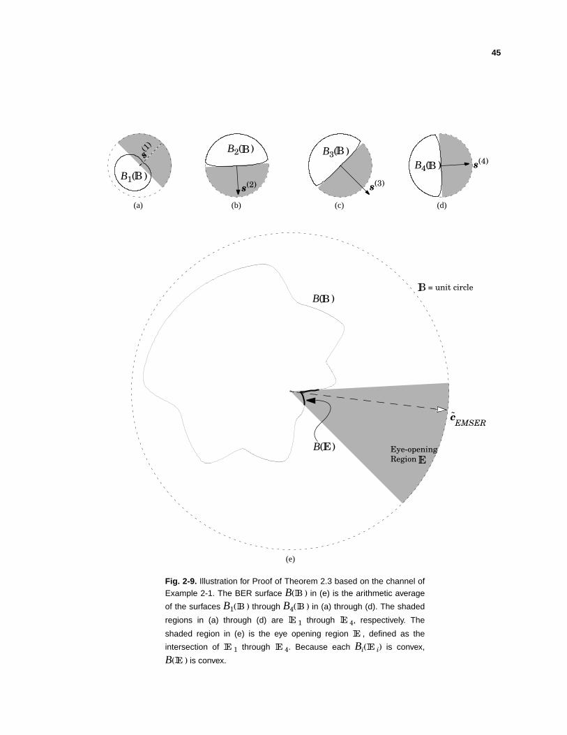
Fig. 2-9. Illustration for Proof of Theorem 2.3 based on the channel ofExample 2-1. The BER surface B( ) in (e) is the arithmetic average
of the surfaces B1( ) through B4( ) in (a) through (d). The shaded
regions in (a) through (d) are 1 through 4, respectively. The
shaded region in (e) is the eye opening region , defined as the
intersection of 1 through 4. Because each Bi( i) is convex,
B( ) is convex.
BB B
E E
EE E E
E
B( )
EMSERc
B1( )
Eye-openingRegion
s(1)
s(2)
B2( )
s(3)
B3( )s(4)B4( )
(a) (b) (c) (d)
(e)
E
B
B
B BB
B = unit circle
B( )E
46
CHAPTER 3
A D A P T I V EE Q U A L I Z A T I O NU S I N G T H E A M B E RA L G O R I T H M
3.1 INTRODUCTION
Although the EMSER algorithm of the previous chapter is useful for finding the min-
imum-SER equalizer of known channels, it is poorly suited for adaptive equalization. We
now propose the approximate minimum-bit-error-rate (AMBER) algorithm for adapting
the coefficients of an equalizer for both PAM and QAM channels. While less complex
than the LMS algorithm, AMBER very nearly minimizes error probability in white Gaus-
sian noise and can significantly outperform the MMSE equalizer when the number of
equalizer coefficients is small relative to the severity of the intersymbol interference.
47
In section 3.2, we approximate the fixed-point relationship of the EMSER equalizer. In
section 3.3, we propose a globally convergent numerical algorithm to recover the solution
to the approximate fixed-point equation. In section 3.4, we transform the numerical algo-
rithm into a stochastic equalizer algorithm, namely the AMBER algorithm. We discuss
some key parameters, such as an error indicator function and an update threshold, of the
AMBER algorithm. We then extend the AMBER algorithm to QAM and DFE. In
section 3.5, we perform computer simulations to evaluate and compare the error proba-
bility performance of the MMSE, the EMSER, and the AMBER equalizers. In addition,
we empirically characterize the ISI channels over which the EMSER and the AMBER
equalizers are more beneficial than the MMSE equalizer. In section 3.6, we summarize our
results.
3.2 FUNCTIONAL APPROXIMATION
As mentioned in chapter 2, by setting to zero the gradient of (2-12) with respect to the
equalizer c, we find that the c minimizing error probability must satisfy the EMSER fixed-
point equation c = af(c) for some a > 0. For convenience, we again state f(c) of (2-22)
here:
f(c) = s(1) + s(2) + … + s(K) , (3-1)
where αi = cTs(i) ⁄(||c|| σ) is a normalized inner product of s(i) with c.
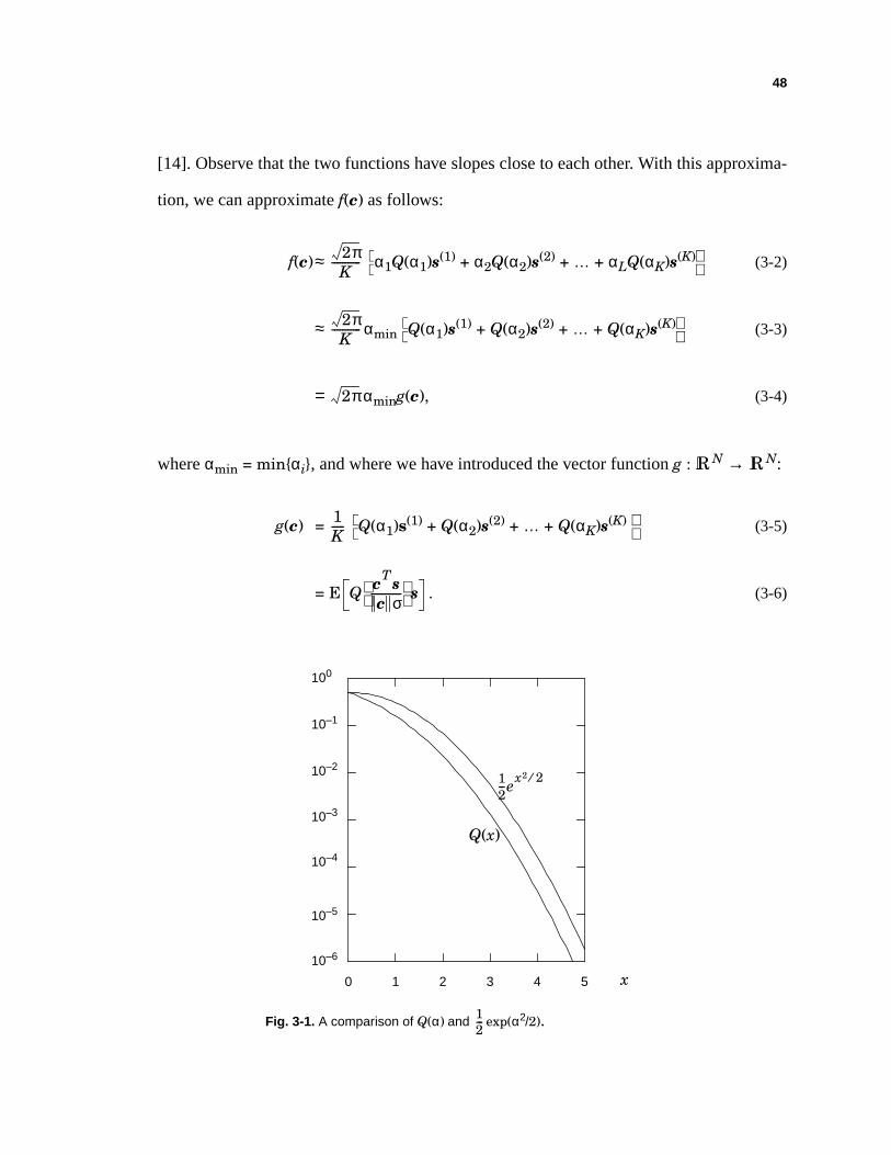
Instead of using the EMSER fixed-point relationship, we use an approximate fixed-
point relationship for reasons that will become apparent later on. Recall that the error
function Q(α) is upper bounded and approximated by 0.5 exp(α2/2), as shown in Fig. 3-1
1K-----
eα1
2– 2⁄e
α22– 2⁄
eαK
2– 2⁄
48
[14]. Observe that the two functions have slopes close to each other. With this approxima-
tion, we can approximate f(c) as follows:
f(c)≈ α1Q(α1)s(1) + α2Q(α2)s(2) + … + αLQ(αK)s(K) (3-2)
≈ αmin Q(α1)s(1) + Q(α2)s(2) + … + Q(αK)s(K) (3-3)
= αming(c), (3-4)
where αmin = min{αi}, and where we have introduced the vector function g : N → N:
g(c) = Q(α1)s(1) + Q(α2)s(2) + … + Q(αK)s(K) (3-5)
= E . (3-6)
2πK
-----------
2πK
-----------
2π
0 1 2 3 4 5
Fig. 3-1. A comparison of Q(α) and exp(α2/2).12---
12--ex2 2⁄
Q(x)
x
100
10–1
10–2
10–3
10–4
10–5
10–6
R R
1K-----
Q cTsc σ
----------- s
49
Comparing (3-1) and (3-5), we see that the vector function g(c) has the same form as f(c),
but with Q(α) replacing exp(– α2 ⁄2). The approximation in (3-3) is valid because only the
terms in (3-2) for which αi ≈ αmin are relevant, and the other terms have negligible impact.
In analogy to the EMSER fixed-point relationship, we define the approximate minimum-
bit-error-rate (AMBER) fixed-point relationship by:
c = ag(c), for some a > 0. (3-7)
We define that the equalizer satisfying (3-7) as the AMBER equalizer. Because Q(⋅) is also
an exponentially decreasing function, (3-5) suggests that g(c) is dictated by only these
signal vectors whose inner products with c are relatively small. Thus, the AMBER equal-
izer will be very nearly a linear combination of the few signal vectors for which the eye
diagram is most closed.
The following theorem shows that, although there may be numerous unit-length solu-
tions to the EMSER fixed-point equation c = af(c) for a > 0, there is only one unit-length
solution to c = ag(c) for a > 0; call it AMBER. This is one obvious advantage of this
approximate fixed-point relationship (3-7) over the EMSER fixed-point relationship (2-
24).
Theorem 3.1: For an equalizable channel there is a unique unit-length vector
AMBER satisfying the AMBER fixed-point relationship of (3-7).
Proof. The proof of Theorem 3.1 is in Appendix 3.1.
We will learn in section 3.4 that a more important advantage of the approximate fixed-
point relationship over the EMSER fixed-point relationship is its amenability to a simple
stochastic implementation.
c
c
50
While the equalizer cAMBER no longer minimizes error probability exactly, the accu-
racy with which Q(x) approximates for large x suggests that cAMBER closely
approximates the EMSER equalizer at high SNR. The simulation results in section 3.5
will substantiate this claim.
3.3 A NUMERICAL METHOD
Recall that we constructed a numerical algorithm to recover solutions to the EMSER
fixed-point relationship of (2-24). To recover solutions to the AMBER fixed-point rela-
tionship, we use a similar approach by proposing the following numerical algorithm:
ck + 1 = ck + µ g(ck), (3-8)
where µ is a positive step size.
Because there exists only one unique solution to c = ag(c) for a > 0, we can prove the
global convergence of this numerical algorithm:
Theorem 3.2: If the channel is equalizable, the numerical algorithm of (3-8) is
guaranteed to converge to the direction of the unique unit-length vector AMBER
satisfying = ag( ) for a > 0.
Proof. The proof of Theorem 3.2 is in Appendix 3.2.
3.4 STOCHASTIC IMPLEMENTATION
As mentioned before, the EMSER algorithm is useful only when the channel is known
and thus is not suitable for stochastic implementation. The main advantage of the numer-
ical algorithm of (3-8) is that there exists a simple stochastic implementation.
12---e x2 2⁄–
c
c c
51
3.4.1 Error Indicator Function
At first glance, (3-8) is only more complicated than the EMSER algorithm of (2-26).
However, the replacement of the exponential function with the Gaussian error function
motivates a simplified adaptation algorithm. Let us first introduce an error indicator func-
tion I(xk–D , yk) to indicate the presence and sign of an error: let I = 0 if no error occurs, let
I = 1 if an error occurs because yk is too negative, and let I = –1 if an error occurs because
yk is too positive. In other words:
I(xk–D , yk) = (3-9)
Thus, we see that the expectation of the squared error indicator function is simply the error
probability:
E[I 2] = E . (3-10)
This equation suggests that there maybe a connection between the error indicator function
and the numerical algorithm of (3-8), where the equalizer is adapted by signal vectors
weighted by their conditional error probabilities. In fact, we can relate the error indicator
function to g(c) by the following theorem:
Theorem 3.3: The error indicator is related to g(c) by
E[I rk] = g(c) – ε(c)c , (3-11)
where ε(c) is a small positive constant.
Proof. The proof of Theorem 3.3 is in Appendix 3.3.
1, if yk < (xk – D – 1)fD and xk – D ≠ – L + 1,
–1 , if yk > (xk – D + 1)fD and xk – D ≠ L – 1,0, otherwise.
2L 2–L
----------------- Q cTsc σ
-----------
2L 2–L
----------------- { }
52
Theorem3.3 allows us to usethe error indicator function to simplify the numerical
algorithm of (3-8) as follows:
ck+1 = ck + µg(ck) (3-12)
= ck + µ(E[I rk] + ε(ck)ck) (3-13)
= (1 + µε(ck))ck + µE[I rk]. (3-14)
≈ ck + µE[I rk], (3-15)
where the approximation in (3-15) is accurate whenµε(c) is small.
Whenthestepsizeµ is significantlysmall,anensembleaveragecanbewell approxi-
matedby a time average,andwe canremove the expectationin (3-15) to yield the fol-
lowing stochastic algorithm:
ck+1 = ck + µ I rk. (3-16)
We referto this stochasticupdateastheapproximate minimum-BER (AMBER) algorithm.
In chapter4 we will address its convergence properties in details.
We remarkthat (3-16)hasthesameform astheLMS algorithm,exceptthat theerror
indicatorfunctionof theLMS is ILMS = xk – D – yk. Observe thatAMBER is lesscomplex
thanLMS because(3-16)doesnot requirea floating-pointmultiplication.Recallthat the
sign-LMS algorithm is
ck+1 = ck + µ Isign-LMS rk, (3-17)
53
where Isign-LMS = sgn(ILMS). AMBER can be viewed as the sign LMS algorithm modi-
fied to update only when a symbol decision error is made.
3.4.2 Tracking of fD
The LMS algorithm penalizes equalizer outputs for deviating away from constellation
points and thus controls the norm of the equalizer so that the main tap of the overall
impulse response is approximately unity, e.g. fD ≈ 1. On the other hand, fD is not neces-
sarily close to unity for the AMBER algorithm.
Knowledge of fD is not needed for binary signaling since the decisions are made based
on the sign of the equalizer outputs. However, for general L-PAM, the value of the indi-
cator function I depends on fD, which changes with time as c is being updated.
To estimate fD, we propose an auxiliary update algorithm. First, we let D(k) denote
the estimate of fD at time k. For a given xk – D, the equalizer output yk equals the sum of
fDxk – D and a perturbation term resulting from residual ISI and Gaussian noise. Since the
perturbation term has zero mean, the mean of the equalizer output is fDxk – D, and that
yk ⁄xk – D has a mean of fD. We can thus track fD using a simple moving average as follows:
D(k + 1) = (1 – λ) D(k) + λ , (3-18)
where λ is a small positive step size. The estimated detection thresholds are then {0,
±2 D(k), …, ±(L – 2) D(k)}.
3.4.3 Update Threshold
Because the AMBER algorithm of (3-16) updates only when an error occurs, i.e. when
the error indicator I ≠ 0, the convergence rate will be slow when the error rate is low. To
f
f fyk
xk D–---------------
f f
54
increase convergence speed, we can modify AMBER so that the equalizer updates not
only when an error is made, but also when an error is almost made, i.e. when the distance
between the equalizer output and the nearest decision threshold is less than some small
positive constant τ. Mathematically, the modified indicator function is
Iτ(xk – D, yk) = (3-19)
Observe that when τ = 0, the modified AMBER algorithm reverts back to (3-16).
We note that the expectation of the squared modified-error-indicator function is no
longer the error probability, but rather
E[Iτ2] = E . (3-20)
The original AMBER algorithm (τ = 0) requires knowledge of xk – D; In other words, it
requires a training sequence. When a training sequence is not available, the original
AMBER algorithm cannot be operated in a decision-directed manner: if decisions are used
in place of actual symbols, the indicator function would be identically zero since it is not
possible for AMBER to tell whether an error has occurred, and hence the equalizer would
never escape from its initial condition. Fortunately, the threshold modification has a
second advantage: besides increasing the convergence speed, the modified algorithm can
also be implemented in a decision-directed manner by using k – D in place of xk – D in (3-
19). Because a decision-directed algorithm cannot recognize when an error is made, the
modified algorithm in decision-directed mode updates only when an error is almost made.
We can expect that the impact of decision errors on this decision-directed algorithm will
be negligible when the error probability is reasonably small, perhaps 10–2 or less.
1, if yk < (xk – D – 1)fD + τ and xk – D ≠ – L + 1,
–1 , if yk > (xk – D + 1)fD – τ and xk – D ≠ L – 1,0, otherwise.
2L 2–L
----------------- Q cTs τ–c σ
------------------
x
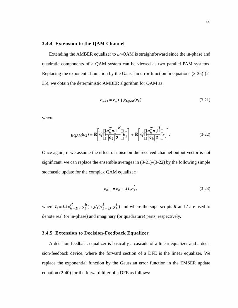
55
3.4.4 Extension to the QAM Channel
Extending the AMBER equalizer to L2-QAM is straightforward since the in-phase and
quadratic components of a QAM system can be viewed as two parallel PAM systems.
Replacing the exponential function by the Gaussian error function in equations (2-35)-(2-
35), we obtain the deterministic AMBER algorithm for QAM as
ck+1 = ck+ µgQAM(ck) (3-21)
where
gQAM(ck) = E + E . (3-22)
Once again, if we assume the effect of noise on the received channel output vector is not
significant, we can replace the ensemble averages in (3-21)-(3-22) by the following simple
stochastic update for the complex QAM equalizer:
ck+1 = ck + µ Iτ , (3-23)
where Iτ = Iτ( , ) + jIτ( , ) and where the superscripts R and I are used to
denote real (or in-phase) and imaginary (or quadrature) parts, respectively.
3.4.5 Extension to Decision-Feedback Equalizer
A decision-feedback equalizer is basically a cascade of a linear equalizer and a deci-
sion-feedback device, where the forward section of a DFE is the linear equalizer. We
replace the exponential function by the Gaussian error function in the EMSER update
equation (2-40) for the forward filter of a DFE as follows:
Qck
Ts1( )R
ck σ----------------------
s1* Q
ckTs j( )
I
ck σ--------------------
s j
rk*
xk D–R yk
R xk D–I yk
I
56
ck+1 = ck + µgfwd(ck, dk), (3-24)
where
gfwd(c, d) = E . (3-25)
Based on the deterministic AMBER update of (3-24), we can then form an almost iden-
tical stochastic update for the forward filter:
ck+1 = ck + µIτrk, (3-26)
where Iτ is the error indicator function evaluating the equalizer outputs after decision feed-
back and rk is the equalizer inputs for the forward filter of the DFE.
As mentioned in section 2.6, the feedback filters of both the MMSE and the EMBER
DFEs are to eliminate post-cursor ISI and we can update the feedback filter of the
AMBER DFE with the LMS algorithm:
dk+1 = dk – µek , (3-27)
where ek is the difference between the DFE output and the desired signal, and where
= [ ... ] is the past data vector and is replaced by the data deci-
sion vector = [ ... ] in the decision-directed mode.
QcTs N2
i D=dixk i–∑–( )
c σ----------------------------------------------------------
s
xk D– 1–
xk D– 1–T xk D– 1– xk N2–
xk D– 1–T xk D– 1– xk N2–
57
3.5 NUMERICAL RESULTS
3.5.1 SER Simulation
In this subsection,we considerseveralexamplesto comparetheSERperformanceof
theEMSER,AMBER, andMMSE equalizers.We alsoplot someeye diagramsof equal-
izer outputs to illustrate the difference between the MMSE and the AMBER equalizers.
Example 3-1: We first considerlinearequalizationfor a binarysignalingchannel
H(z) = 1.2 + 1.1z–1 – 0.2z– 2. In Fig. 3-2 we plot BER versusSNR = hk2 ⁄σ2,
consideringtheMMSE, EMSER,andAMBER equalizersof lengththreeandfive.
With threeequalizertapsanda delayof D = 2, the AMBER equalizerhasa more
than6.5 dB gain over theMMSE equalizer. With five tapsandD = 4, theAMBER
equalizerhasanearly2 dB gainoverMMSE. Observe thattheAMBER (solid)and
EMSER (dashed)curves are nearly indistinguishable.In Fig. 3-3, we present
“artificial” noiselesseyepatternsfor theEMSER,AMBER, andMMSE equalizers,
assumingfive equalizertapsand SNR = 30 dB. Thesepatternsare obtainedby
interpolatingall possiblenoiselessequalizeroutputswith a triangularpulseshape.
All equalizersare normalizedto have identical norm (and thus identical noise
enhancement).The EMSER and AMBER eye patternsare virtually identical,
whereasthe MMSE eye patternis drasticallydifferent.The interestingdifference
betweenthe MMSE and AMBER equalizersresultsfrom the MMSE equalizer’s
effort to forceall possibleequalizeroutputsto { ±1}, despitethebenefitsof sparing
the outputs with large noise immunity.
Σk
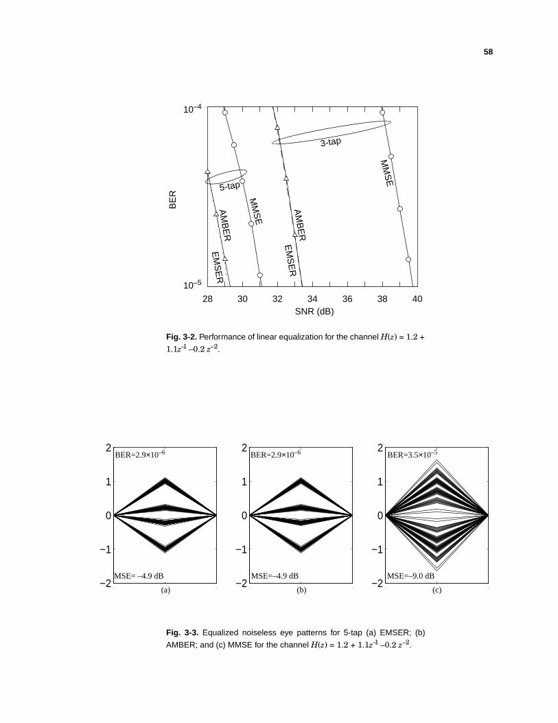
58
28 30 32 34 36 38 40
10–5
10–4
MM
SE
EM
SE
RA
MB
ER
MM
SE
AM
BE
RE
MS
ER
SNR (dB)
BE
R
3-tap
5-tap
Fig. 3-2. Performance of linear equalization for the channel H(z) = 1.2 +1.1z–1 – 0.2 z– 2.
0 1 2−2
−1
0
1
2
0 1 2−2
−1
0
1
2
0 1 2−2
−1
0
1
2
(a) (b) (c)
MSE= –4.9 dB
BER=2.9×10⁻⁶
MSE=–4.9 dB
BER=2.9×10⁻⁶ BER=3.5×10⁻⁵
MSE=–9.0 dB
Fig. 3-3. Equalized noiseless eye patterns for 5-tap (a) EMSER; (b)
AMBER; and (c) MMSE for the channel H(z) = 1.2 + 1.1z–1 – 0.2 z– 2.
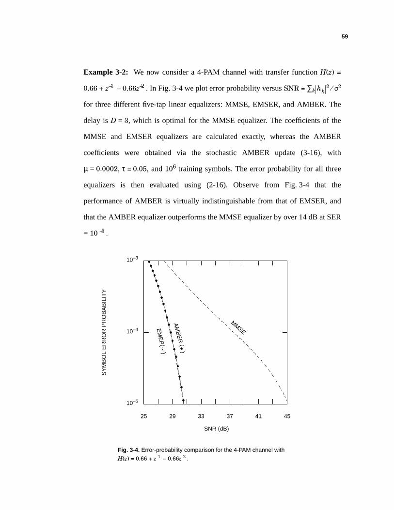
59
Example 3-2: We now considera 4-PAM channelwith transferfunction H(z) =
0.66 + z–1 – 0.66z–2 . In Fig. 3-4 weplot errorprobabilityversusSNR = ∑k2 ⁄ σ2
for threedifferentfive-taplinear equalizers:MMSE, EMSER,andAMBER. The
delay is D = 3, which is optimal for the MMSE equalizer. The coefficientsof the
MMSE and EMSER equalizersare calculatedexactly, whereasthe AMBER
coefficients were obtained via the stochastic AMBER update (3-16), with
µ = 0.0002, τ = 0.05, and106 training symbols.The error probability for all three
equalizers is then evaluated using (2-16). Observe from Fig. 3-4 that the
performanceof AMBER is virtually indistinguishablefrom that of EMSER,and
thattheAMBER equalizeroutperformstheMMSE equalizerby over14dB atSER
= 10 –5 .
hk
Fig. 3-4. Error-probability comparison for the 4-PAM channel with
H(z) = 0.66 + z–1 – 0.66z–2 .
MMSE
AM
BE
R(
)
SNR (dB)
SY
MB
OL
ER
RO
R P
RO
BA
BIL
ITY
EM
EP
(---)
25 29 33 37 41 45
10–5
10–4
10–3
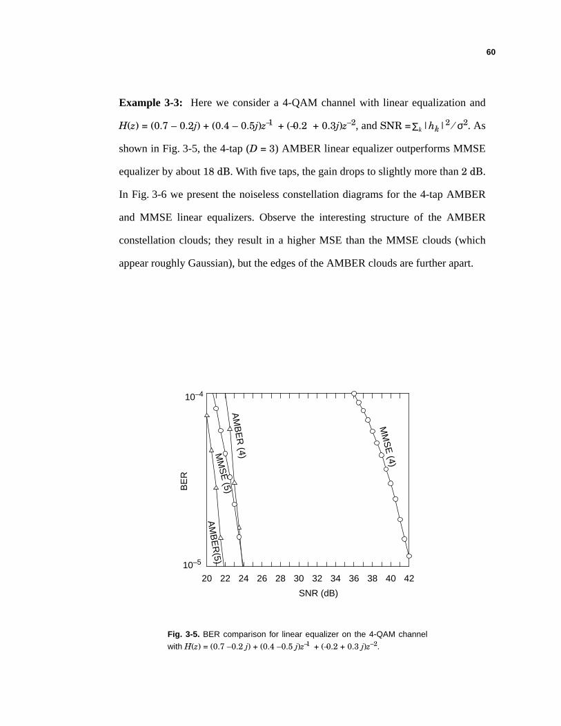
60
Example 3-3: Here we consider a 4-QAM channel with linear equalization and
H(z) = (0.7 – 0.2j) + (0.4 – 0.5j)z–1 + (–0.2 + 0.3j)z– 2, and SNR = |hk|2 ⁄σ2. As
shown in Fig. 3-5, the 4-tap (D = 3) AMBER linear equalizer outperforms MMSE
equalizer by about 18 dB. With five taps, the gain drops to slightly more than 2 dB.
In Fig. 3-6 we present the noiseless constellation diagrams for the 4-tap AMBER
and MMSE linear equalizers. Observe the interesting structure of the AMBER
constellation clouds; they result in a higher MSE than the MMSE clouds (which
appear roughly Gaussian), but the edges of the AMBER clouds are further apart.
Σk
20 22 24 26 28 30 32 34 36 38 40 42
MM
SE
(4)
AM
BE
R (4)M
MS
E (5)
AM
BE
R(5)
SNR (dB)
BE
R
10–5
10–4
Fig. 3-5. BER comparison for linear equalizer on the 4-QAM channel
with H(z) = (0.7 – 0.2 j) + (0.4 – 0.5 j)z–1 + (–0.2 + 0.3 j)z– 2.
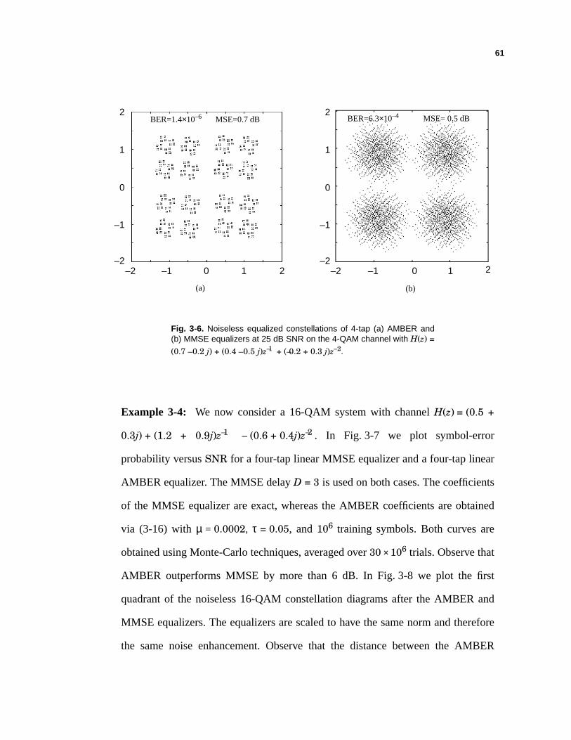
61
Example 3-4: We now consider a 16-QAM system with channel H(z) = (0.5 +
0.3j) + (1.2 + 0.9j)z–1 – (0.6 + 0.4j)z–2 . In Fig. 3-7 we plot symbol-error
probability versus SNR for a four-tap linear MMSE equalizer and a four-tap linear
AMBER equalizer. The MMSE delay D = 3 is used on both cases. The coefficients
of the MMSE equalizer are exact, whereas the AMBER coefficients are obtained
via (3-16) with µ = 0.0002, τ = 0.05, and 106 training symbols. Both curves are
obtained using Monte-Carlo techniques, averaged over 30 × 106 trials. Observe that
AMBER outperforms MMSE by more than 6 dB. In Fig. 3-8 we plot the first
quadrant of the noiseless 16-QAM constellation diagrams after the AMBER and
MMSE equalizers. The equalizers are scaled to have the same norm and therefore
the same noise enhancement. Observe that the distance between the AMBER
(a) (b)
–2 0
–1
–2–1 1
2
0
1
2
–1
–2
2
0
1
–2 0–1 1 2
MSE= 0.5 dBBER=6.3×10⁻⁴MSE=0.7 dBBER=1.4×10⁻⁶
Fig. 3-6. Noiseless equalized constellations of 4-tap (a) AMBER and(b) MMSE equalizers at 25 dB SNR on the 4-QAM channel with H(z) =(0.7 – 0.2 j) + (0.4 – 0.5 j)z–1 + (–0.2 + 0.3 j)z– 2.
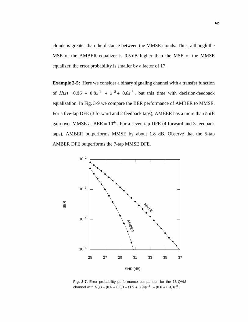
62
clouds is greater than the distance between the MMSE clouds. Thus, although the
MSE of the AMBER equalizer is 0.5 dB higher than the MSE of the MMSE
equalizer, the error probability is smaller by a factor of 17.
Example 3-5: Here we consider a binary signaling channel with a transfer function
of H(z) = 0.35 + 0.8z–1 + z– 2 + 0.8z–3 , but this time with decision-feedback
equalization. In Fig. 3-9 we compare the BER performance of AMBER to MMSE.
For a five-tap DFE (3 forward and 2 feedback taps), AMBER has a more than 5 dB
gain over MMSE at BER = 10–5 . For a seven-tap DFE (4 forward and 3 feedback
taps), AMBER outperforms MMSE by about 1.8 dB. Observe that the 5-tap
AMBER DFE outperforms the 7-tap MMSE DFE.
Fig. 3-7. Error probability performance comparison for the 16-QAM
channel with H(z) = (0.5 + 0.3j) + (1.2 + 0.9j)z–1 – (0.6 + 0.4j)z–2 .
SNR (dB)
AM
BE
R
MM
SE
25 27 29 31 33 35 37
10–5
10–4
10–3
10–2
SE
R
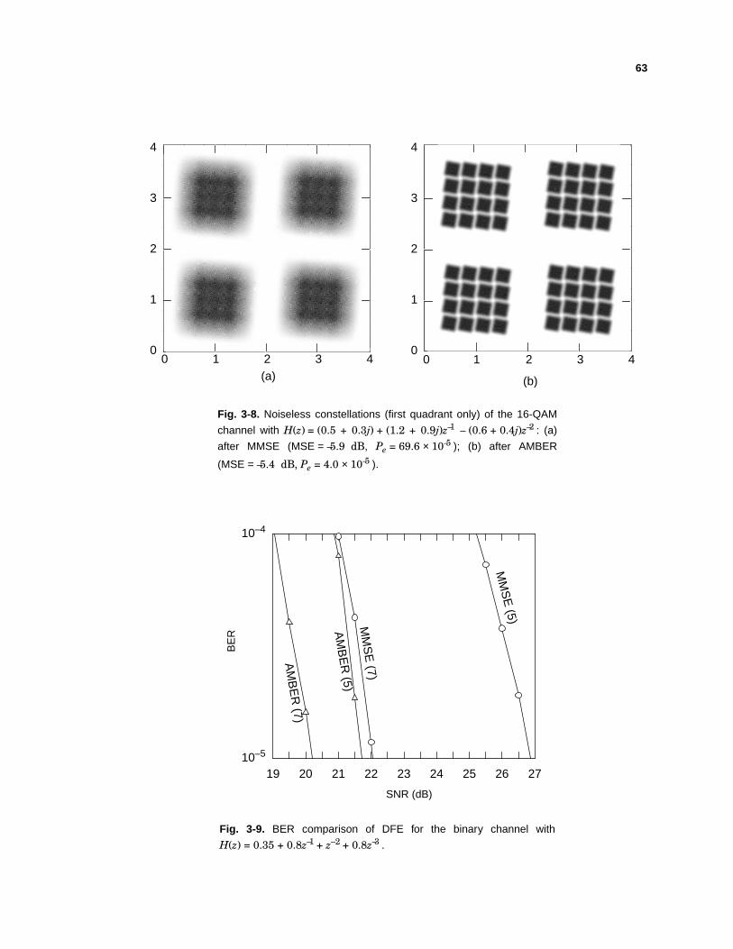
63
50 100 150 200 250 300 350 400 450 500
50
100
150
200
250
300
350
400
450
50050 100 150 200 250 300 350 400 450 500
50
100
150
200
250
300
350
400
450
500
(a) (b)
0 2 40
2
4
1 30 2 41 3
1
3
0
2
4
1
3
Fig. 3-8. Noiseless constellations (first quadrant only) of the 16-QAM
channel with H(z) = (0.5 + 0.3j) + (1.2 + 0.9j)z–1 – (0.6 + 0.4j)z–2 : (a)
after MMSE (MSE = –5.9 dB, Pe = 69.6 × 10⁻⁵ ); (b) after AMBER
(MSE = –5.4 dB, Pe = 4.0 × 10⁻⁵ ).
19 20 21 22 23 24 25 26 2710–5
10–4
SNR (dB)
BE
RM
MS
E (5)
AM
BE
R (5)
MM
SE
(7)
AM
BE
R (7)
Fig. 3-9. BER comparison of DFE for the binary channel with
H(z) = 0.35 + 0.8z–1 + z– 2 + 0.8z–3 .
64
3.5.2 ISI Channel Characterization
Basedon our simulationresultsin the previous subsection,we suspectthat without
enoughequalizertaps,theAMBER (andtheEMSER)equalizersarelikely to significantly
outperformthe MMSE equalizerson severe ISI channels.However, the above claim is
rathervagueandmoreconcretescenariosareneededto quantifytheclaim. In this subsec-
tion wedeviseanISI channelcharacterizationprocedureto identify scenariosin which the
AMBER and the EMSER equalizers significantly outperform the MMSE equalizer.
We have realizedfrom our previoussimulationresultsthatdrasticallydifferenterror-
probabilityperformancesarereflectedin theeyediagrams.Morespecifically, themorethe
MMSE eyepatternis closed,themorepotentialis theAMBER equalizerto improveerror
probability performance.As we have mentionedearlier, the noiselesseye pattern is
formed by plotting the noiselessequalizeroutputsand equivalently, the inner products
betweentheequalizerandthesignalvectors.We will now give two rules-of-thumbbased
on our empirical observations.
Rule 1. For an MMSE equalizer, if its smallestoutput is significantly lessthanthe
desiredsignal(e.g. thesmallestnoiselessequalizeroutputis 0.1 andthedesiredsignal
is 1), thenit is possible to have theAMBER andtheEMSERequalizerssignificantly
outperform the MMSE equalizer.
Rule 2. If someMMSE equalizeroutputs,which significantly closethe eye of the
channel,have largedispersion,thentheAMBER andtheEMSERequalizersarepossi-
ble to have large SNR gains over the MMSE equalizer.
65
Of course the above rules do not always hold, but they are in general good. We now
design a crude characterization procedure to predict the SNR gains of the n-tap AMBER
and EMSER equalizers over the n-tap MMSE equalizer.
Step 1. Given a channel, compute the n-tap MMSE equalizer at a high SNR. Obtain
noiseless equalizer outputs by convolving the channel and the MMSE equalizer.
Step 2. Of all the MMSE equalizer outputs corresponding to xk–D = 1, pick one tenth
with smallest values and average them. The predicted SNR gain of the AMBER and
the EMSER equalizers over the MMSE equalizer is
SNRgain = 20 log10 , (3-28)
where OUTavg is the average of the one tenth MMSE equalizer outputs with the smallest
values and OUTsmallest is the smallest MMSE equalizer output. At very high SNR, the
smallest of equalizer outputs dictates the error probability performance; Thus OUTsmallest
is the effective signal strength for the MMSE equalizer at high SNR. On the other hand,
we have observed that both the AMBER and the EMSER equalizers tend to passively
“cluster” equalizer output into sub-clusters, and OUTavg is used to roughly estimate the
mean of the sub-cluster that nearly closes the eye of the channel. The predicted SNR gains
of the AMBER and the EMSER equalizers over the MMSE equalizer are thus the ratios of
OUTavg over OUTsmallest in decibels.
In Fig. 3-10, we plot the actual versus the predicted SNR gains of the EMSER equal-
izers over the MMSE equalizer. With various equalizer taps and two hundred equalizable
3-tap and 4-tap channels, we perform simulations to find the actual SNR gains of the
EMSER equalizer over the MMSE equalizer at error probability less than 10–6 . In general,
OUTavgOUTsmallest-----------------------------------
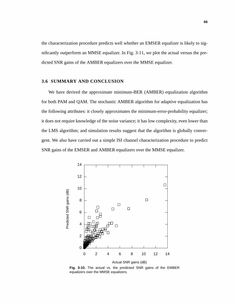
66
the characterization procedure predicts well whether an EMSER equalizer is likely to sig-
nificantly outperform an MMSE equalizer. In Fig. 3-11, we plot the actual versus the pre-
dicted SNR gains of the AMBER equalizers over the MMSE equalizer.
3.6 SUMMARY AND CONCLUSION
We have derived the approximate minimum-BER (AMBER) equalization algorithm
for both PAM and QAM. The stochastic AMBER algorithm for adaptive equalization has
the following attributes: it closely approximates the minimum-error-probability equalizer;
it does not require knowledge of the noise variance; it has low complexity, even lower than
the LMS algorithm; and simulation results suggest that the algorithm is globally conver-
gent. We also have carried out a simple ISI channel characterization procedure to predict
SNR gains of the EMSER and AMBER equalizers over the MMSE equalizer.
Fig. 3-10. The actual vs. the predicted SNR gains of the EMBERequalizers over the MMSE equalizers.
0 2 4 6 8 10 12 14
0
2
4
6
8
10
12
14
Actual SNR gains (dB)
Pre
dict
ed S
NR
gai
ns (
dB)
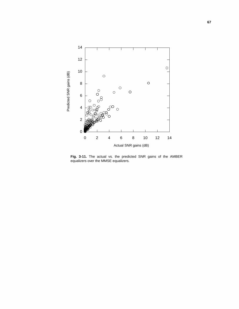
67
0 2 4 6 8 10 12 14
0
2
4
6
8
10
12
14
Fig. 3-11. The actual vs. the predicted SNR gains of the AMBERequalizers over the MMSE equalizers.
Actual SNR gains (dB)
Pre
dict
ed S
NR
gai
ns (
dB)

68
APPENDIX 3.1
P R O O F O FT H E O R E M 3 . 1
In this appendix, we prove Theorem 3.1: For any equalizable channel there is a unique
unit-length vector, AMBER, satisfying the fixed-point relationship = ag( ) for a > 0.
By contradiction: suppose both 1 and 2 satisfy = ag( ), a > 0, where
|| 1 || = || 2 || = 1. Let P denote the plane containing the origin and the perpendicular
bisector of 1 and 2, as shown in Fig. 3-12 for a three-tap equalizer. This plane bisects
the signal cone S = {Σi ais(i) : ai ³≥ 0} into two subcones A and B, so that S = A ∪ B,
where A is the intersection of S with the set of vectors on the 1 side of P, excluding P,
and B is the intersection of S with the set of vectors on the 2 side of P, including P.
Observe that 1 ∈ A and 2 ∈B and that A and B are disjoint, A ∩ B = ∅.
From (3-5), g( 1) can be decomposed into two summations over signal vectors from A
and B:
c c c
c c c c
c c
c c
c
c
c c
c
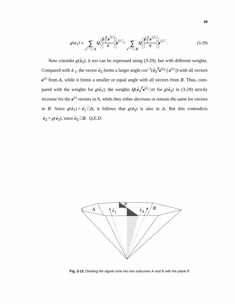
69
g( 1) = . (3-29)
Now consider g( 2); it too can be expressed using (3-29), but with different weights.
Compared with 1, the vector 2 forms a larger angle cos–1( 2Ts(i)⁄|| s(i) ||) with all vectors
s(i) from A, while it forms a smaller or equal angle with all vectors from B. Thus, com-
pared with the weights for g( 1), the weights Q( 2Ts(i) ⁄σ) for g( 2) in (3-29) strictly
increase for the s(i) vectors in A, while they either decrease or remain the same for vectors
in B. Since g( 1) = 1 ∈A, it follows that g( 2) is also in A. But this contradicts
2 = g( 2), since 2 ∈B. Q.E.D.
c Qc1
Ts i( )
σ----------------
s i( ) A∈∑ s i( ) Q
c1Ts j( )
σ-----------------
s j( )
s j( ) B∈∑+
c
c c c
c c c
c c c
c c c
Fig. 3-12. Dividing the signal cone into two subcones A and B with the plane P.
A Bc1 c2
P
70
APPENDIX 3.2
P R O O F O FT H E O R E M 3 . 2
In this appendix,we prove Theorem3.2. Let s(i) be the i-th of the LM+N–1 possible
signalvectors.Sincethe channelis equalizable,all s(i) vectorsform a conesuchthat we
canfind a vectorhaving anangleof strictly lessthan90° with all s(i) vectors.Becausethe
s(i) vectorsform acone,wecanfind ahyperplaneP, containingtheorigin, suchthatall s(i)
vectorsarestrictly ononesideof P. Everys(i) makesanangleθi ∈[0, 90°) with thenormal
to P andconsistsof two components:one(with norm||s(i)||sinθ) parallelto P andtheother
(with norm||s(i)||cosθ) perpendicularto P. At eachupdate,thecorrectionvectorµg(ck) is
strictly inside the cone and its norm is lower boundedby µQ(||s ||max ⁄ σ)||s ||minsinθmin,
where||s||min = mini{||s (i)||}, ||s ||max = maxi{||s (i)||}, andθmax = maxi{θi}. At iterationM + 1,
thesumof thepastM correctionvectorsis a vectorstrictly insidetheconeandhasa norm
of at leastMµQ(||s ||max ⁄ σ)||s ||minsinθmin. We concludethat, for any initial c0 with a finite
71
norm, there exists a finite M such that cM+1 is strictly inside the cone. In addition, we con-
clude that || ck || grows without bound as k increases.
Showing that ck converges to the direction of a solution satisfying c = ag(c) for a > 0
is equivalent to showing that the angle between ck and g( k) approaches zero, where
k = ck ⁄ || ck ||. Because ||ck|| grows without bound while the norm of the update, || µg( k)||,
is upper-bounded by µ|| s ||max, it follows that k must converge to some fixed vector ∞, so
that g( k) converges to g( ∞). Thus, for any ε > 0, there exists a finite k(ε) such that for all
k > k(ε), | || g( k)|| – ||g( ∞)|| | ≤ ||g( k) – g( ∞)|| < ε. Manipulating the inequalities yields
that the angle between g( k) and g( ∞) is less than some θ(ε), where
θ(ε) = cos–1 . (3-30)
For any M > 0, g( k(ε) + j) is a vector strictly within the cone W[g( ∞); θ(ε)] con-
sisting of all vectors forming an angle of less than θ(ε) with g( ∞). For a ck(ε) with finite
norm, we can find a finite M such that ck(ε) + M is strictly inside W[g( ∞); θ(ε)]. As ε
approaches 0, θ(ε) approaches 0 and thus the angle between ck(ε) + M and g( k(ε) + M)
approaches 0 as well. Q.E.D.
c
c c
c c
c c
c c c c
c c
1 ε q c∞( )⁄–
1 ε q c∞( )⁄+------------------------------------
j 0=
M 1–∑ c c
c
c
c
72
APPENDIX 3.3
P R O O F O FT H E O R E M 3 . 3
This appendix proves Theorem 3.3: The ensemble average E[Isk] is the same as
E[IHxk] or HE[Ixk]. We equivalently derive the ensemble average E[Ixk] by finding the
scalar E[Ixk – D] and the vector E[Iz] where we have defined the vector z = [xk, …, xk–D+ 1,
xk–D– 1, …, xk–M–N+ 1]T by discarding the (D + 1)-st component of xk.
Let “left”, “right”, and “inner” denote the events of xk–D = – L +1, xk–D = L – 1, and
xk–D ∈{±1, ±3, …, ±(L– 3)}, respectively. (If L = 2, “inner” is the null event.) Then:
E[Ixk–D ] = E[Ixk–D |left]P[left] + E[Ixk–D |right]P[right] + E[Ixk–
D|inner]P[inner] (3-31)
= E[I|left] + E[I|right] + E[Ixk–D |inner]. (3-32)L– 1+L
------------------L 1–
L------------- L 2–
L-------------
73
But I is independent of xk–D when xk–D is an inner point, so that the last term is zero:
E[I xk–D |inner] = E[I|inner]E[xk–D |inner] = E[I|inner] × 0 = 0. (3-33)
Thus, (3-32) reduces to:
E[I xk–D ] = –E[ I|left] + E[I|right] (3-34)
= – (–P[ bTz + cTnk > fD]) + P[bTz + cTnk < – fD] (3-35)
= E + E (3-36)
= E . (3-37)
We thus have the surprising result that the ensemble average E[I xk–D ] does not depend
on xk–D ! We have defined the vector b = [f0, …, fD– 1, fD+1, …, fM+N– 1]T by discarding the
(D + 1)-st component of f. The last equality follows because z and – z have the same dis-
tribution. The derivation of E[Iz] is as follows:
E[Iz] = E[Iz|left] + E[Iz|right] + E[Iz|inner] (3-38)
= E E[I|z, left]z + E[I|z, right]z + (L – 2)E[I|z, inner]z (3-39)
= E – Q z + Q z +
(L – 2) Q – Q z (3-40)
L 1–L
-------------
L 1–L
-------------
L 1–L
-------------
Qf D bTz–
c σ------------------------
Qf D bTz+
c σ------------------------
2L 2–L
----------------- Qf D bTz+
c σ-----------------------
1L---- 1
L---- L 2–
L-------------
1L----
1L----
f D bTz–
c σ------------------------
f D bTz+
c σ------------------------
f D bTz+
c σ------------------------
f D bTz–
c σ------------------------
74
= E – E (3-41)
= E . (3-42)
The ensemble E[Iz] does not depend on xk – D either. Combining (3-37) and (3-42), we
have
E[Ixk] = E (3-43)
and
E[Isk] = E[IHxk] = E (3-44)
where is a random vector with distribution p( ) = p(xk|xk – D = 1), i.e., is uniformly
distributed over the set of LM+N – 1 L-ary xk vectors for which xk – D = 1 and = H .
We now derive the ensemble average E[Ink]. We first partition E[Ink] into three condi-
tional expectation terms as follows:
E[Ink] = E[Ink|I = 1, z = zl] P[I = 1, z = zl] +
E[Ink|I = – 1, z = zl] P[I = – 1, z = zl] +
E[Ink|I = 0, z = zl] P[I = 0, z = zl], (3-45)
where each term is summed over LM+N – 1 possible z vectors. Note that the last summation
term in (3-45) is a zero vector since I = 0 and Ink = 0. We first concentrate on the first
summation term in (4-18) by finding the conditional expectation E[Ink|I = 1, z = zl] and
the joint probability P[I = 1, z = zl]. Here we determine E[Ink|I = 1, z = zl]:
L 1–L
------------- Qf D bTz+
c σ------------------------
z L 1–L
------------- Qf D bTz–
c σ------------------------
z
2L 2–L
----------------- Qf D bTz+
c σ------------------------
z
2L 2–L
----------------- Q cTH xc σ
---------------- x
2L 2–L
----------------- Q cT sc σ
------------ s
x x x
s x
l∑
l∑
l∑
75
E[Ink|I = 1, z = zl] = E[nk|I = 1, z = zl] (3-46)
= E[nk|cTnk < – fD – bTzl, xk – D ≠ – L + 1] (3-47)
= E[nk|cTnk < – fD – bTzl]. (3-48)
Let U be any unitary matrix with first column equal to the unit-norm equalizer vector
c ⁄|| c ||. Then = UTnk has the same statistics as nk, namely, the components of are
i.i.d. zero-mean Gaussian with variance σ2. Furthermore, cTU = || c ||e1, where
e1 = [1 0 0 … 0], and nk = U . Continuing on (3-48), we have
E[Ink|I = 1, z = zl] = E[U |cTU < – fD – bTzl] (3-49)
= UE[ ||| c || < – fD – bTzl] (3-50)
= UE | > (3-51)
= – σUE | > e1 (3-52)
= – σE c ⁄|| c ||, (3-53)
where we have introduced the function
m(η) = E[X | X ≥ η], (3-54)
where X is a zero-mean unit-variance Gaussian random variable. We now derive the joint
probability P[I = 1, z = zl]:
P[I = 1, z = zl]= P[I = 1|z = zl] P[z = zl] (3-55)
n n
n
n n
n n1
nn1–
σ---------
f D bTzl+c σ
-------------------------
n1–
σ---------
n1–
σ---------
f D bTzl+c σ
-------------------------
mf D bTzl+
c σ-------------------------
e η2– 2⁄
2πQ η( )------------------------- =∆
76
= . (3-56)
Combining (3-53) and (3-56), the first summation term in (3-45) becomes
E[Ink|I = 1, z = zl] P[I = 1, z = zl]
= (3-57)
= (3-58)
= . (3-59)
It is not hard to show that
E[Ink|I = 1, z = zl] P[I = 1, z = zl]
= E[Ink|I = – 1, z = zl] P[I = – 1, z = zl], (3-60)
and therefore, we conclude that
E[Ink] = – . (3-61)
Q.E.D.
L 1–L
-------------Qf D bTzl
+
c σ--------------------------
1
LM N 1–+--------------------------
l∑
l∑ L 1–( )σ–
LM N+ 2π----------------------------
f D bTzl+( )
2–
2 c 2σ2-------------------------------------
expcc-------
L 1–( )σ–L 2π
------------------------Ef D bTz+( )
2–
2 c 2σ2-----------------------------------
expcc-------
L 1–( )σ–L 2π
------------------------E cT s( )2
–
2 c 2σ2---------------------
expcc-------
l∑
l∑
2L 2–L
-----------------σ2π
----------E cT s( )2
–
2 c 2σ2---------------------
expcc-------
77
CHAPTER 4
C O N V E R G E N C EA N A L Y S I S
4.1 INTRODUCTION
In the previous chapter, we proposed a low-complexity stochastic equalizer algorithm
(AMBER) that very nearly minimizes error probability. In this chapter, we discuss its
global convergence properties and propose a variant to increase its convergence speed.
Assuming the equalizer coefficients vary slowly (which is true for a sufficiently small
step size), a stochastic equalizer update can then be expected to follow a deterministic tra-
jectory [15]. In this chapter, we first derive the ensemble average of the stochastic
AMBER algorithm to approximate its time average in order to study its mean convergence
behavior. Because of the highly complicated and nonlinear nature of the update dynamics,
instead of a rigorous mathematical proof, we describe the likely global convergence prop-
erty of the AMBER algorithm and propose a global convergence conjecture based on sim-
78
ulation results and some analytical understanding on the update dynamics. Finally, we
propose a variant with faster convergence speed.
4.2 ENSEMBLE AVERAGE OF AMBER
The AMBER algorithm proposed in the previous chapter is
ck+1 = ck + µIτrk, (4-1)
whose ensemble average can be derived by taking expectation of both sides of (4-1). The
deterministic trajectory of the equalizer coefficients is described by
ck+1 = ck + µE[Iτrk] (4-2)
= ck + µE[Iτsk] + µE[Iτnk], (4-3)
where we separate the noisy channel output vector rk into the noiseless channel output
vector sk and the noise vector nk. We now find the ensemble averages E[Iτsk] and E[Iτnk].
Theorem 4.1: The ensemble average of the AMBER algorithm of (4-2) is
ck+1= ck + µE – µ . (4-4)
Proof. The proof of Theorem 4.1 is in Appendix 4.1.
4.3 GLOBAL CONVERGENCE PROPERTY
Having derived the ensemble average of the AMBER algorithm in the previous sec-
tion, we now discuss the global convergence property of AMBER by analyzing the deter-
Qck
T s τ–
ck σ-------------------
s σ2π
----------Eck
T s τ–( )2
–
2 ck2σ2
-------------------------------
expckck
----------
79
ministic trajectory of the equalizer coefficient vector. From the results of the previous
section, the ensemble average of the stochastic AMBER algorithm is
ck+1= ck + µ1E[Iτrk]
= ck + µ1E[Iτsk] + µ1E[Iτnk]
= ck + µE – µ , (4-5)
where µ = µ1. Rearranging (4-5), we get
ck+1 = ck + . (4-6)
By inspection, we see that when the step size µ is chosen sufficiently small, the norm of
the equalizer in (4-6) is shrunk by some positive factor (less than 1) before the equalizer
vector is adjusted by the steering term . We denote the vector term
as the shrinking vector since it reduces the equalizer norm.
Before we analyze the convergence property, we would like to point out from (4-5)
that the equalizer update stops, or ck+1 = ck, when the steering term equals the shrinking
term:
= . (4-7)
The equilibrium condition of (4-7) directly implies: (1) the steering vector points in the
same direction as the equalizer vector when the equalizer converges, and (2) the magni-
tudes (or norms) of the steering vector and the shrinking vector are the same.
Qck
T s τ–
ck σ-------------------
s σ2π
----------Eck
T s τ–( )2
–
2 ck2σ2
-------------------------------
expckck
----------
2L 2–L
-----------------
1 µσ2π ck
----------------------Eck
T s τ–( )–2
2 ck2σ2
------------------------------
exp–
µE Qck
T s τ–
ck σ-------------------
s
E Qck
T s τ–
ck σ-------------------
sσ2π
----------Eck
T s τ–( )2–
2 ck2σ2---------------------------
expckck
----------
E Qck
T s τ–
ck σ-------------------
s σ2π
----------Eck
T s τ–( )2
–
2 ck2σ2
------------------------------
expckck
----------
80
4.3.1 The Locus
Recall that the original AMBER (τ = 0) equalizer is uniquely characterized by the
fixed-point relationship c = ag(c) for some a > 0, where only the direction of c matters.
However, for τ > 0, the norm of c matters as well. We now define a new fixed-point rela-
tionship:
c = gτ(c) (4-8)
where
gτ(c) = . (4-9)
Following the proof in Appendix 3.1 which shows that there is a unique unit-length vector
satisfying the fixed-point relationship c = ag(c) for some a > 0, it is not hard to show that
for a positive number M, there exists a unique equalizer with equalizer norm M satisfying
the new fixed-point relationship of (4-8).
When the norm of c is very small relative to τ, the term is essentially
, or (Q(w) ≈ 1 when w << 0). c = simply means that c is the
average of all signal vectors. On the other hand, when the norm of c is very large relative
to τ, we have gτ(c) ≈ g(c) since the effect of τ in (4-9) is effectively eliminated by the large
denominator.
Geometrically, the new fixed-point relationship defines a locus of equalizer vector c
parameterized by τ. Given a channel, a noise variance σ2, and an update threshold τ, we
can form a locus realizing (4-8) by plotting the norm and the direction of c for all values of
||c|| ≥ 0.
cgτ c( )
-------------------
E Q cT s τ–c σ
------------------- s
E Q cT s τ–c σ
------------------- s
E Q τ–c σ
------------ s E s[ ] E s[ ]
81
Example 4-1: Here we use a two-tap equalizer to illustrate a locus. We consider a
two-tap binary-signaling channel where the channel has a transfer function H(z) = –
0.6 + z–1 . In this example, we use SNR = 10 dB and τ = 0.1. In Fig. 4-1, we plot
three different-norm equalizer vectors satisfying (4-8). The dashed circles are
circles whose radii are the norms of the equalizers. We see these vectors point in
three different directions. In Fig. 4-2, we plot the locus by connecting all equalizers
(with norms from 0.001 to 2.0) satisfying (4-8). We see that the portion on locus
corresponding to large equalizer norms is nearly a straight line, whereas when the
equalizer norm is small, the effect of τ makes the initial curvy segment of the locus.
It is harder to visualize a locus when we consider equalizers with more than two taps
since the locus would then live in a higher dimensional space. We now attempt to describe
a locus in an intuitive way: A N-dimensional space is occupied by a N-dimensional onion
with the center of the onion at the origin of the space. The onion has infinite layers of skin,
each skin layer is a hollow hypersphere with a certain radius. In Fig. 4-1 and Fig. 4-2, the
dashed circles are the onion skin layers in the two-dimensional space. As demonstrated
Fig. 4-1, for each skin layer, there is a hole pierced by a unique vector whose norm is the
radius of the layer and whose direction is characterized by (4-8). The locus is like a thread
passing through the holes of all skin layers of the onion as seen in Fig. 4-2.
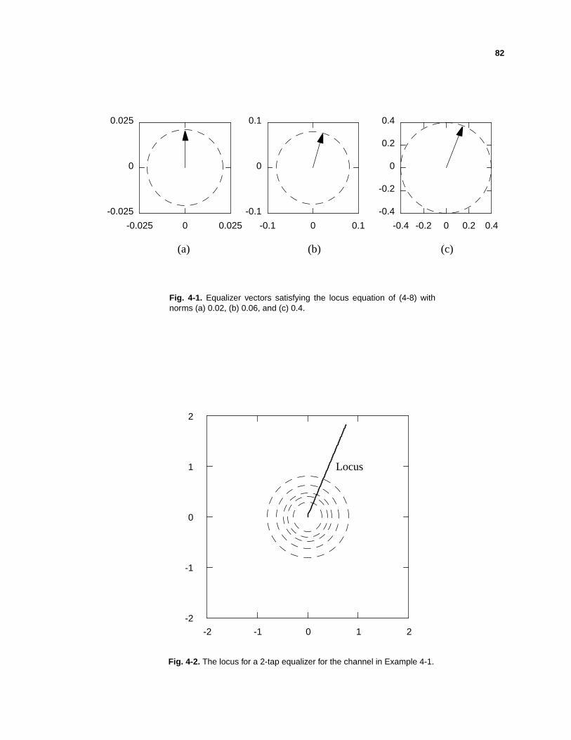
82
Fig. 4-1. Equalizer vectors satisfying the locus equation of (4-8) withnorms (a) 0.02, (b) 0.06, and (c) 0.4.
-0.1 0 0.1
-0.1
0
0.1
-0.4 -0.2 0 0.2 0.4
-0.4
-0.2
0
0.2
0.4
-0.025 0 0.025
-0.025
0
0.025
(a) (c)(b)
Fig. 4-2. The locus for a 2-tap equalizer for the channel in Example 4-1.
-2 -1 0 1 2-2
-1
0
1
2
Locus
83
4.3.2 Global Convergence
In thissubsection,weconjecturethattheAMBER algorithmconvergesgloballywith a
sufficiently small stepsize.To substantiateour conjecture,we first studytheequilibrium
state of AMBER with the following claim:
Lemma 4-1: Theequilibriumstatedescribedby (4-7) cannotbetruefor a c with
anarbitrarylargeor smallnorm.In addition,thereexistssomec with a finite non-
zero norm satisfying the equilibrium state.
Proof. The proof for Lemma 4-1 is in Appendix 4.2.
We now investigate whetherthe AMBER algorithm indeedconvergesglobally. We
startwith theconceptof thehyperspaceonion.For any positive numberM, thereexistsa
hollow hypersphere(onion skin layer) with radiusM and thereexists a uniquevector
c*(M) with norm M satisfying the fixed-point relationshipof (4-8). We now make the
claimthatthelocusactsasan“attractor”whichattractstheupdatetowardsit, startingwith
the following lemma:
Lemma 4-2: If ck andc*(||ck||) form anangleφ, thereexistsa sufficiently small
stepsizeµ suchthattheanglebetweenck+1 andc*(||ck||) is strictly smallerthenφ.
Proof. The proof for Lemma 4-2 is in Appendix 4.3.
Conjecture: In order to formally claim that the updatebecomesasymptotically
closerto the locus,we needto show that theanglebetweenck+1 andc*(||ck+1||) is
lessthan the anglebetweenck and c*(||ck||). Although it hasn’t beenrigorously
proved,simulationresultsin section4.5 have shown that the rateof changeof the
enclosedanglebetweenc*(||ck||) andc*(||ck+1||) is slower thanthe rateof change
84
of the enclosed angle between ck and ck+1 and thus we conjecture that the update
trajectory gets closer to the locus for a sufficiently small update step size.
We observe that once the update trajectory gets close enough to the locus, the equal-
izer update process is more norm adjusting (expanding or shrinking the equalizer norm to
reach the equilibrium state) than direction adjustment. We will substantiate our claim with
computer simulation results in section 4.5.
4.4 MULTI-STEP ALGORITHMS
The update frequency, and consequently the convergence speed, of the original
AMBER (τ = 0) is proportional to error probability. Although we have incorporated an
update threshold τ to increase its convergence speed, a further increase in convergence
speed may still be possible.
It is well known that the recursive least-squared (RLS) algorithm [7] yields the fastest
convergence speed and the best steady-state MSE performance. One may be tempted to
ask this question: what is the best algorithm in terms of convergence speed and steady-
state error-probability performance (closest to the minimum error probability)?
Unfortunately, the counterpart of the RLS algorithm in the minimum error probability
criterion is difficult to find. Nevertheless, we recognize that by simply varying the step size
of an update algorithm, we can increase the convergence speed. Instead of finding the best
error-probability-based algorithm to maximize speed of convergence, here we attempt to
give a reasonably good step size function to improve convergence speed.
Recall that the error indicator function of AMBER is binary (either there is an update
or there is no update), and the expectation of the error indicator function is the Gaussian
error function. It relies on a long training sequence in order to approach its expectation.
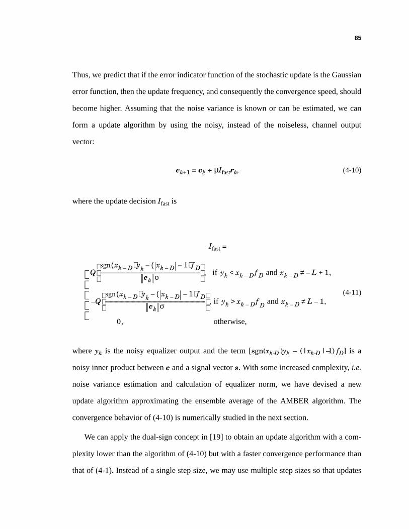
85
Thus, we predict that if the error indicator function of the stochastic update is the Gaussian
error function, then the update frequency, and consequently the convergence speed, should
become higher. Assuming that the noise variance is known or can be estimated, we can
form a update algorithm by using the noisy, instead of the noiseless, channel output
vector:
ck+1 = ck + µIfastrk, (4-10)
where the update decision Ifast is
Ifast =
(4-11)
where yk is the noisy equalizer output and the term [sgn(xk–D )yk – (|xk–D |–1) fD] is a
noisy inner product between c and a signal vector s. With some increased complexity, i.e.
noise variance estimation and calculation of equalizer norm, we have devised a new
update algorithm approximating the ensemble average of the AMBER algorithm. The
convergence behavior of (4-10) is numerically studied in the next section.
We can apply the dual-sign concept in [19] to obtain an update algorithm with a com-
plexity lower than the algorithm of (4-10) but with a faster convergence performance than
that of (4-1). Instead of a single step size, we may use multiple step sizes so that updates
Q
xk D–( ) ysgn k xk D– 1–( ) f D–
ck σ----------------------------------------------------------------------------------
, if yk xk D– f D and xk D– L– 1,+≠<
Q–xk D–( ) ysgn k xk D– 1–( ) f D–
ck σ----------------------------------------------------------------------------------
, if yk xk D– f D and xk D– L 1,–≠>
0, otherwise,
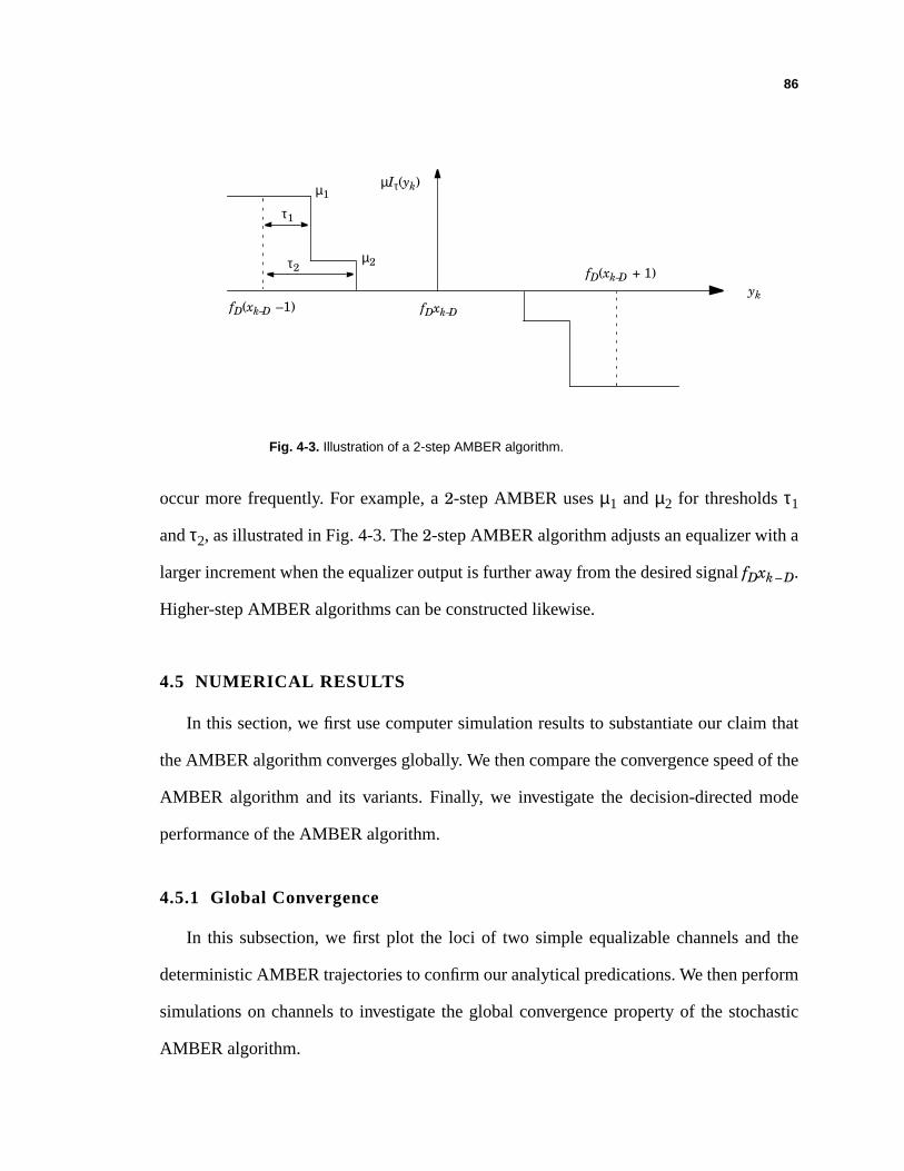
86
occur more frequently. For example, a 2-step AMBER uses µ1 and µ2 for thresholds τ1
and τ2, as illustrated in Fig. 4-3. The 2-step AMBER algorithm adjusts an equalizer with a
larger increment when the equalizer output is further away from the desired signal fDxk – D.
Higher-step AMBER algorithms can be constructed likewise.
4.5 NUMERICAL RESULTS
In this section, we first use computer simulation results to substantiate our claim that
the AMBER algorithm converges globally. We then compare the convergence speed of the
AMBER algorithm and its variants. Finally, we investigate the decision-directed mode
performance of the AMBER algorithm.
4.5.1 Global Convergence
In this subsection, we first plot the loci of two simple equalizable channels and the
deterministic AMBER trajectories to confirm our analytical predications. We then perform
simulations on channels to investigate the global convergence property of the stochastic
AMBER algorithm.
fDxk–D
fD(xk–D + 1)
fD(xk–D – 1)
τ1
τ2µ2
µ1
yk
µIτ(yk)
Fig. 4-3. Illustration of a 2-step AMBER algorithm.
87
We first use the simple channel H(z) = –0.6 + z–1 from Example 4-1. For visualization
purpose, we update a two-tap equalizer so that we can plot the update trajectory in a two-
dimensional space. We use SNR = 10 dB and τ = 0.1. In Fig. 4-4, we plot the locus and the
trajectory with the initial condition [–2, 1]. In Fig. 4-5, we plot the locus and the trajectory
with the initial condition [–1, –1]. The equilibrium point is [0.2031, 0.5014].
We substantiate our claim with another simple channel: H(z) = 0.4 + z–1 – 0.2z–2 .
With SNR = 10 dB and τ = 0.1. In Fig. 4-6, we plot the locus and the update trajectory
with the initial condition [–1, –1]. In Fig. 4-7, we plot the locus and the trajectory with the
initial condition [1, 1]. The equilibrium point is [–0.2278, 0.6629] .
As predicted by our analytical reasoning in section 4.3, the deterministic trajectories
from above two examples first approach the loci and then “slide” along the loci to reach
the equilibrium points.
Besides observing the deterministic trajectories of the ensemble averaged AMBER
algorithm, we also perform computer simulations to substantiate our claim on the global
convergence property of the stochastic AMBER algorithm. We pick one hundred equaliz-
able three-tap ISI channels, whose taps are distributed uniformly between -1 and 1, and
apply three-tap equalizers. All equalizers are initialized with small random numbers. All
equalizers converge closely to their minimum-error-probability solutions. For each
channel, we first find the EMSER solution and thus find the minimum-SER value. Each
equalizer learning curve is plotted with time k versus SERk/SERmin. Instead of plotting
one hundred different equalizer learning curves, we average the one hundred learning
curves and plot the averaged learning curve in Fig. 4-8. All equalizers use a step size of µ
= 0.0001 and a threshold of τ = 0.1.

88
Fig. 4-4. The locus and the 2-tap equalizer trajectory (with initial
condition [-2, 1]) for the channel H(z) = –0.6 + z–1 .
-2 -1 0 1 2
-2
-1
0
1
2
-2 -1 0 1 2
-2
-1
0
1
2
Trajectory Locus
Equilibrium Point
Initial Point
Fig. 4-5. The locus and the trajectory (with initial condition [–1, –1]) for
the channel H(z) = –0.6 + z–1 .
-2 -1 0 1 2
-2
-1
0
1
2
-2 -1 0 1 2
-2
-1
0
1
2
Locus
Equilibrium Point
Initial Point
Traj
ecto
ry
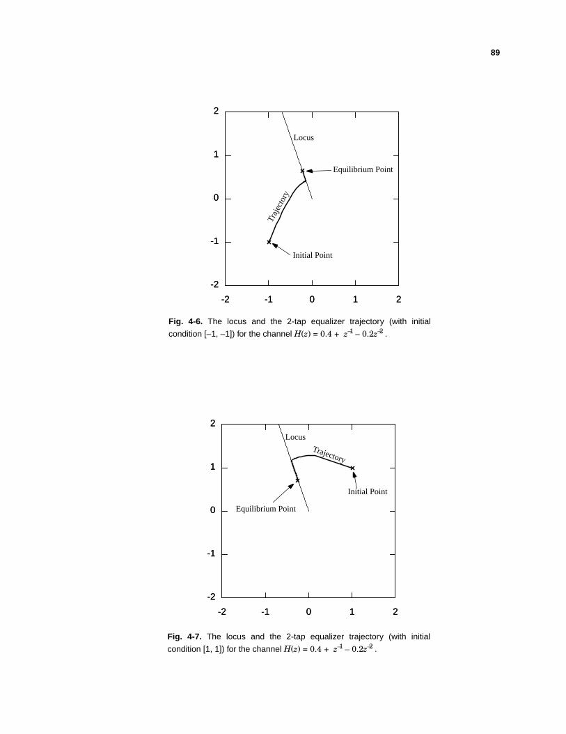
89
Fig. 4-6. The locus and the 2-tap equalizer trajectory (with initial
condition [–1, –1]) for the channel H(z) = 0.4 + z–1 – 0.2z–2 .
-2 -1 0 1 2
-2
-1
0
1
2
-2 -1 0 1 2
-2
-1
0
1
2
Locus
Equilibrium Point
Initial Point
Traj
ecto
ry
Fig. 4-7. The locus and the 2-tap equalizer trajectory (with initial
condition [1, 1]) for the channel H(z) = 0.4 + z–1 – 0.2z–2 .
-2 -1 0 1 2
-2
-1
0
1
2
-2 -1 0 1 2
-2
-1
0
1
2
Initial Point
Equilibrium Point
LocusTrajectory
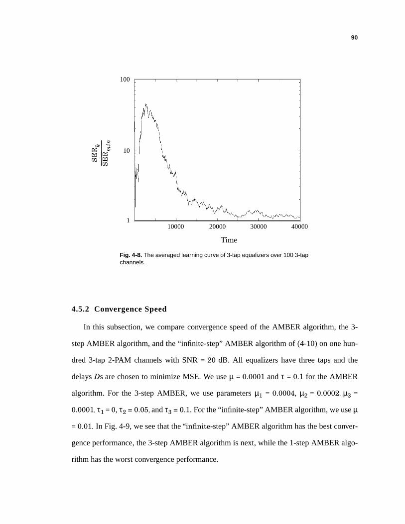
90
4.5.2 Convergence Speed
In this subsection, we compare convergence speed of the AMBER algorithm, the 3-
step AMBER algorithm, and the “infinite-step” AMBER algorithm of (4-10) on one hun-
dred 3-tap 2-PAM channels with SNR = 20 dB. All equalizers have three taps and the
delays Ds are chosen to minimize MSE. We use µ = 0.0001 and τ = 0.1 for the AMBER
algorithm. For the 3-step AMBER, we use parameters µ1 = 0.0004, µ2 = 0.0002, µ3 =
0.0001, τ1 = 0, τ2 = 0.05, and τ3 = 0.1. For the “infinite-step” AMBER algorithm, we use µ
= 0.01. In Fig. 4-9, we see that the “infinite-step” AMBER algorithm has the best conver-
gence performance, the 3-step AMBER algorithm is next, while the 1-step AMBER algo-
rithm has the worst convergence performance.
Fig. 4-8. The averaged learning curve of 3-tap equalizers over 100 3-tapchannels.
10000 4000030000200001
10
100
SE
Rk
SE
Rm
in----
--------
--------
---
Time
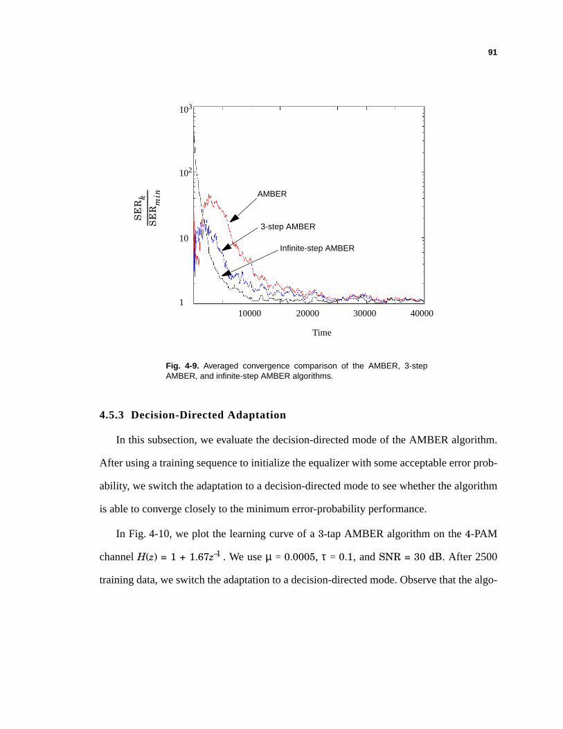
91
4.5.3 Decision-Directed Adaptation
In this subsection, we evaluate the decision-directed mode of the AMBER algorithm.
After using a training sequence to initialize the equalizer with some acceptable error prob-
ability, we switch the adaptation to a decision-directed mode to see whether the algorithm
is able to converge closely to the minimum error-probability performance.
In Fig. 4-10, we plot the learning curve of a 3-tap AMBER algorithm on the 4-PAM
channel H(z) = 1 + 1.67z–1 . We use µ = 0.0005, τ = 0.1, and SNR = 30 dB. After 2500
training data, we switch the adaptation to a decision-directed mode. Observe that the algo-
Fig. 4-9. Averaged convergence comparison of the AMBER, 3-stepAMBER, and infinite-step AMBER algorithms.
10000 400003000020000
Time
1
10
102
SE
Rk
SE
Rm
in----
--------
--------
---
103
AMBER
3-step AMBER
Infinite-step AMBER
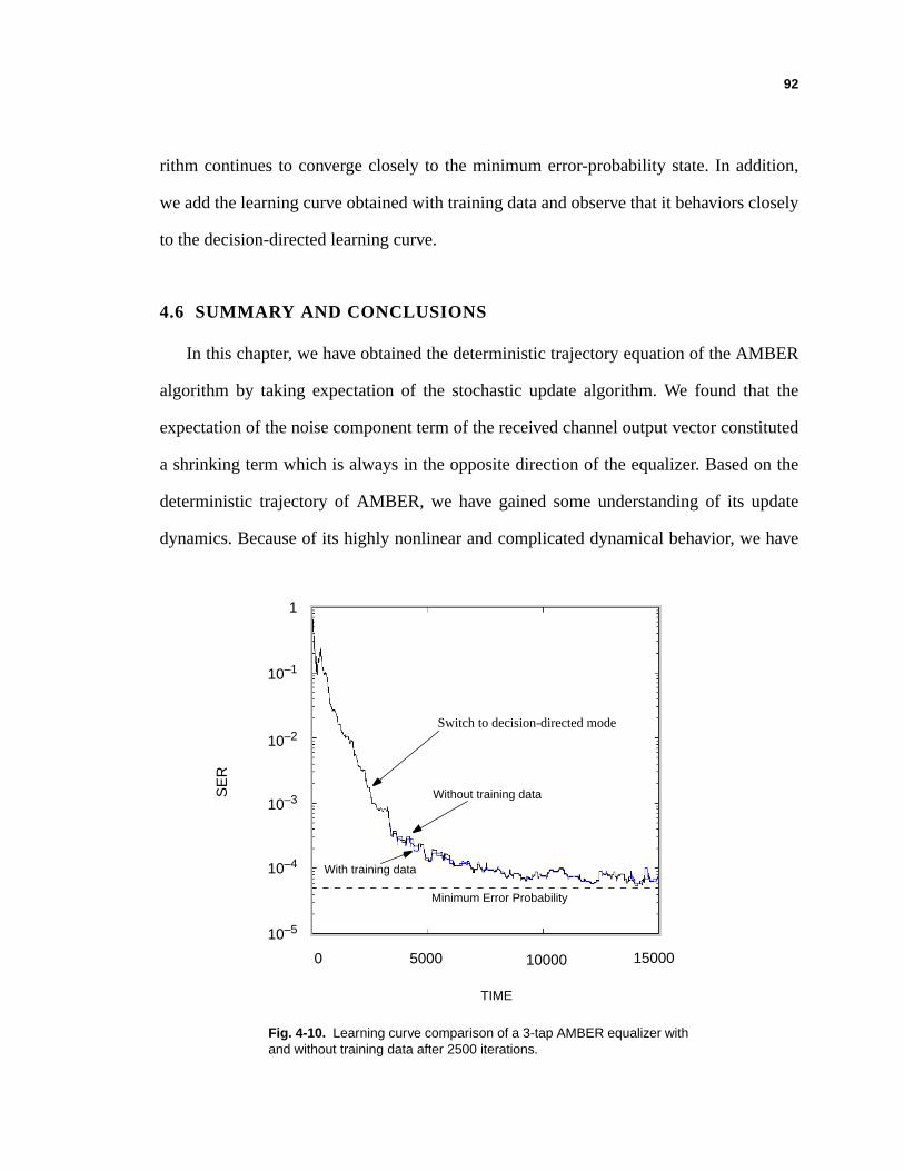
92
rithm continues to converge closely to the minimum error-probability state. In addition,
we add the learning curve obtained with training data and observe that it behaviors closely
to the decision-directed learning curve.
4.6 SUMMARY AND CONCLUSIONS
In this chapter, we have obtained the deterministic trajectory equation of the AMBER
algorithm by taking expectation of the stochastic update algorithm. We found that the
expectation of the noise component term of the received channel output vector constituted
a shrinking term which is always in the opposite direction of the equalizer. Based on the
deterministic trajectory of AMBER, we have gained some understanding of its update
dynamics. Because of its highly nonlinear and complicated dynamical behavior, we have
Fig. 4-10. Learning curve comparison of a 3-tap AMBER equalizer withand without training data after 2500 iterations.
0 5000 10000 15000
10–5
10–4
10–3
10–2
10–1
1
TIME
SE
R
Minimum Error Probability
Switch to decision-directed mode
With training data
Without training data

93
not been able to rigorously prove global convergence. However, we can qualitatively pre-
dict the nonlinear dynamics. Further, we have substantiated our claim of the global con-
vergence property with computer simulation results.
In addition to the discussion on the global convergence, we have proposed a multi-step
variant of AMBER to increase convergence speed. We have shown that the “infinite-tap”
AMBER equalizer converges rather quickly at a cost of some complexity increase. By
incorporating the ideas of the dual-sign algorithm and the continuous function of the
expected error indicator function, we have used variable step sizes to increase update fre-
quency and convergence speed.
94
APPENDIX 4.1
P R O O F O FT H E O R E M 4 . 1
In this appendix, we prove Theorem 4.1. This proof closely follows the proof in
Appendix 3.3 and will only be sketched here.
We first find the ensemble average E[Iτxk] by finding the scalar E[Iτxk – D] and the
vector E[Iτz] where z = [xk, …, xk–D+ 1, xk–D– 1, …, xk–M–N+ 1]T.
Following the notations in Appendix 3.3, we have:
E[Iτxk–D ] = E[Iτ|left] + E[Iτ|right] (4-12)
= E + E (4-13)
= E , (4-14)
L– 1+L
------------------L 1–
L-------------
L 1–L
-------------
Qf D bTz– τ–
c σ---------------------------------
Qf D bTz τ–+
c σ---------------------------------
2L 2–L
----------------- Qf D bTz τ–+
c σ--------------------------------
95
where b = [f0, …, fD– 1, fD+1, …, fM+N– 1]T. The derivation of E[Iτz] is similar to the deriva-
tion of E[Iz] in Appendix 3.3 and is:
E[Iτ z]= E . (4-15)
Combining (4-14) and (4-15), we have
E[Iτxk] = E (4-16)
and
E[Iτsk] = E[IτHxk] = E (4-17)
where is a random vector with distribution p( ) = p(xk|xk – D = 1), i.e., is uniformly
distributed over the set of LM+N – 1 L-ary xk vectors for which xk – D = 1 and = H .
Again, following the derivation of E[I nk] in Appendix 3.3, the ensemble average
E[Iτnk] is
E[Iτnk] = E[Iτnk|Iτ = 1, z = zl] P[Iτ = 1, z = zl] +
E[Iτnk|Iτ = – 1, z = zl] P[Iτ = – 1, z = zl], (4-18)
where the conditional expectation E[Iτnk|Iτ = 1, z = zl] is:
E[Iτnk|Iτ = 1, z = zl] = – σE c ⁄ || c ||, (4-19)
where the function m(η) is defined in (3-54).
2L 2–L
----------------- Qf D bTz τ–+
c σ---------------------------------
z
2L 2–L
----------------- Q cTH x τ–c σ
------------------------- x
2L 2–L
----------------- Q cT s τ–c σ
------------------- s
x x x
s x
l∑
l∑
mf D bTzl τ–+
c σ---------------------------------
96
We now derive the joint probability P[Iτ = 1, z = zl]:
P[Iτ = 1, z = zl]= P[Iτ = 1|z = zl] P[z = zl] (4-20)
= . (4-21)
Combining (4-19) and (4-21), the first summation term in (4-18) becomes
E[Iτnk|Iτ = 1, z = zl] P[Iτ = 1, z = zl] = . (4-22)
It is not hard to show that
E[Iτnk|Iτ = 1, z = zl] P[Iτ = 1, z = zl]
= E[Iτnk|Iτ = – 1, z = zl] P[Iτ = – 1, z = zl], (4-23)
and thus
E[Iτnk] = – . (4-24)
Q.E.D.
L 1–L
-------------Qf D bTzl τ–+
c σ-----------------------------------
1
LM N 1–+--------------------------
l∑ L 1–( )σ–
L 2π------------------------E cT s τ–( )
2–
2 c 2σ2----------------------------
expcc-------
l∑
l∑
2L 2–L
-----------------σ2π
----------E cT s τ–( )2
–
2 c 2σ2-------------------------------
expcc-------

97
APPENDIX 4.2
P R O O F O FL E M M A 4 - 1
In this appendix, we prove Lemma 4-1: The equilibrium state described by (4-7)
cannot be true for a c with an arbitrary large or small norm. In addition, there exists some
c with a finite non-zero norm satisfying (4-7).
Recall that a locus depicts norms and directions of equalizers satisfying the fixed-point
relationship of (4-8). However, not all equalizers on the locus satisfy (4-7). For referencing
convenience, here we again state the equilibrium condition of (4-7):
= . (4-25)
Here we show that an equalizer c (on the locus) with an arbitrary large or small norm
cannot satisfy (4-25). In order for (4-25) to be true, the norms of both sides have to be
E Q cT s τ–c σ
------------------- s σ
2π----------E cT s τ–( )
2–
2 c 2σ2---------------------------
expcc
-------
98
equal. We see that when an equalizer satisfies (4-25), the norm of the left hand side term in
(4-25) is
= = . (4-26)
since the vector and the unit-norm vector are in the same direction
and their inner product equals the norm of . The norm of the right hand
side term in (4-25) is simply
= . (4-27)
Thus, the equilibrium point(s) on a locus needs to satisfies both (4-25) and the fol-
lowing norm equality:
= . (4-28)
Now if is arbitrarily large, the effect of τ in (4-28) is zero and the left hand side
term of (4-28) effectively becomes , and the right hand side term of (4-
28) becomes , and we will show that the two terms cannot be equal
under the assumption that c opens the eye of the channel (i.e. the inner products > 0).
Let and use the fact that is strictly a upper bound for
Q(w), we prove the following inequality:
= (4-29)
< (4-30)
E Q cT s τ–c σ
------------------- s cT
c------- E Q cT s τ–c σ
------------------- s E Q cT s τ–
c σ-------------------
cT sc----------
E Q cT s τ–c σ
------------------- s cT
c-------
E Q cT s τ–c σ
------------------- s
σ2π
----------E cT s τ–( )2
–
2 c 2σ2---------------------------
expcc
------- σ2π
----------E cT s τ–( )2
–
2 c 2σ2---------------------------
exp
E Q cT s τ–c σ
------------------- cT s
c----------σ2π
----------E cT s τ–( )2
–
2 c 2σ2---------------------------
exp
c
E Q cT sc σ
----------- cT s
c----------
σ2π
----------E cT s( )2
–
2 c 2σ2---------------------
exp
cT s
cT sc σ
----------- w=1
2πw---------------- w–
2
2----------
exp
E Q cT sc σ
----------- cT s
c σ----------- E Q w( )w[ ]
12π
-----------E w–2
2----------
exp
99
= . (4-31)
Thus, the existence of an equalizer with an arbitrarily large norm is not possible at equilib-
rium. We now show the existence of an equalizer with an arbitrarily small norm is not pos-
sible at equilibrium. As , the effect of τ in (4-28) dominates the term and the
left hand side of (4-28) effectively becomes , or ( ≈ 1 if w
<< 0), and the right hand side of (4-28) effectively becomes or 0
( ≈ 0 if w << 0).
We now prove that there exists some c satisfying (4-25). Let Z be the difference
between the two norms of (4-28):
Z = – . (4-32)
We see that Z is a continuous function of c. Since Z < 0 when is arbitrarily large and Z
> 0 when is arbitrarily small, we conclude that there exists some c with a finite non-
zero norm which yields Z = 0 and thus, satisfies the equilibrium state. Q.E.D.
12π
-----------E cT s( )–2
2 c 2σ2---------------------
exp
c 0→ cT s
E Q τ–c σ
----------- cT s
c---------- E cT sc---------- Q w( )
σ2π
----------E τ2–
2 c 2σ2---------------------
exp
w( )exp
E Q cT s τ–c σ
------------------- cT s
c----------σ2π
----------E cT s τ–( )2
–
2 c 2σ2------------------------------
exp
c
c
100
APPENDIX 4.3
P R O O F O FL E M M A 4 - 2
In this appendix, we prove Lemma 4-2: There exists a sufficiently small step size such
that if ck and c*(||ck||) form an angle φ, then the angle between ck+1 and c*(||ck||) is
strictly smaller then φ.
Without loss of generality, we sketch a three-dimensional space example (a 3-tap
equalizer) in Fig. 4-11 and Fig. 4-12. The sphere in Fig. 4-11 has a radius of and
c*(||ck||) is the unique vector, with the norm , satisfying (4-8). The darker shaded cir-
cular cone has a base angle of φ, and has c*(||ck||) at its center and ck at its perimeter. The
lighter shaded irregular cone is the signal cone as discussed in chapter 2.
In Fig. 4-12, we plot the top cross-sectional view of the cones. Let P denote the plane
containing the origin and the perpendicular bisector of ck and c*(||ck||). This plane divides
the signal cone S = {Σi ai(i) : ai ≥ 0} into two subcones A and B, so that S = A ∪ B,
ck
ck
s
101
where A is the intersection of S with the set of vectors on the c*(||ck||) side of P, excluding
P, and B is the intersection of S with the set of vectors on the ck side of P, including P.
Observe that c*(||ck||) ∈ A and ck ∈B and that A and B are disjoint, A ∩ B = ∅.
The function gτ(c*(||ck||)) can be decomposed into two weighted summations over
signal vectors from A and B:
gτ(c*(||ck||)) ∝ . (4-33)
Instead of gτ(c*(||ck||)), we look at gτ(ck); it too can be expressed using (4-33), but
with different weights. Compared with c*(||ck||), the vector ck forms a larger angle with
all vectors s(i) from A, while it forms a smaller or equal angle with all vectors from B.
Thus, compared with the weights for gτ(c*(||ck||)), the weights for gτ(ck) in (4-33) strictly
increase for the s(i) vectors in A, while they either decrease or remain the same for vectors
in B. Since gτ(c*(||ck||)) ∝ c*(||ck||)∈ A, it follows that gτ(ck) is also in A as shown in
Fig. 4-12. The vector ck+1 is a linear combination of ck and gτ(ck) and can be made inside
the circular cone if the step size is sufficiently small. Thus, the angle between ck+1 and
c*(||ck||) is less than the angle between ck and c*(||ck||). Q.E.D.
Qc* ck( )T s i( ) τ–
c1 σ-------------------------------------------
s i( ) A∈∑ s i( ) Q
c* ck( )T s j( ) τ–
c1σ--------------------------------------------
s j( )
s j( ) B∈∑+
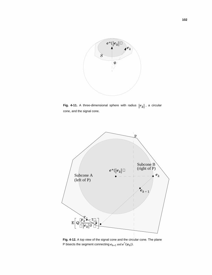
102
ck
c* ck( )
φ
Fig. 4-11. A three-dimensional sphere with radius , a circular
cone, and the signal cone.
ck
S
ck
ck 1+
E Qck
T s τ–
ck σ-------------------
s
Fig. 4-12. A top view of the signal cone and the circular cone. The plane
P bisects the segment connecting ck+1 and c*(||ck||).
P
Subcone A
Subcone B
(left of P)
(right of P)c* ck( )
103
CHAPTER 5
A P P R O X I M A T EM I N I M U M - B E RM U L T I U S E RD E T E C T I O N
5.1 INTRODUCTION
Previous chapters have been devoted to deriving and evaluating the minimum error-
probability equalizers. In this chapter, we will extend the results on minimum-error-proba-
bility equalization to multiuser detection.
The class of linear multiuser detectors (which includes the conventional matched filter
(MF), decorrelator, and MMSE detectors) is particularly attractive because it offers the
advantages of low complexity, ease of adaptation, and the ability to operate in a decentral-
ized fashion, meaning that only a single user of interest need be demodulated. While the
104
MMSE detectoris widely regardedasa goodmultiuserdetector, a better— indeed,the
best — linear multiuser detectorwould chooseits coefficients so as to minimize the
resulting error probability.
Lupas and Verdú [4] proposed the maximum asymptotic-multiuser-efficiency
(MAME) lineardetectorwhich minimizesBER in the limit asthenoiseapproacheszero.
An adaptive algorithm for realizing the MAME detectoris not yet available. Adaptive
algorithmsfor realizingthe minimum-BERmultiuserdetectorwereproposedin [5] and
[6], but they areeitherhigh in complexity or requireknowledgeof thesignaturesequence
of theuserof interest.TheAMBER multiuserdetectorproposedherehaslow complexity
and does not require knowledge of the signature sequence of user of interest.
This chapteris organizedasfollows. In section5.2,we presenttheproblemstatement.
In section5.3, we discussthe exact minimum-BER (EMBER) multiuser detection.In
section5.4,we proposetheapproximateminimum-BER(AMBER) multiuserdetector. In
section5.5, we presentnumericalresultscomparingthe AMBER, MMSE, decorrelator,
and MF detectors.
5.2 MEMORYLESS MULTIUSER CHANNELS
Theessentialfeaturesof themultiuserdetectionproblemarecapturedby thesynchro-
nous CDMA channel model in which the receiver observation waveform is given by
r(t) = Ai si(t – kT) + n(t), (5-1)
whereN is thenumberof active users,si(t) is theunit-energy receivedsignaturesequence
for useri, Ai is thereceivedamplitudefor useri, ∈{ ±1} is theinformationbit for user
i 1=
N
∑k ∞–=
∞
∑ bki( )
bki( )
105
i during bit-epoch k, and n(t) is additive white Gaussian noise with PSD σ2. Assume that
the signature sequence for user i is of the direct-sequence form
si(t) = di(j)p(t – jT ⁄ m), (5-2)
where M is the number of chips per baud, p(t) is a unit-energy Nyquist chip pulse-shape,
and di = [di(1) … di
(M)]T is a unit-norm vector representing the spreading code for user i.
The receiver may generate sufficient statistics by passing r(t) through a filter matched
to the chip-pulse shape and sampling the output at the chip rate, which leads to the fol-
lowing equivalent discrete-time memoryless model:
rk = Hbk + nk, (5-3)
where H = [d1 d2 … dN]A has dimension M × N, A = diag(Ai), bk = [ … ]T, and
nk is white Gaussian noise with PSD σ2I. A decentralized linear multiuser detector for
user i is then characterized by an M-vector c and the decision rule:
= sgn{cTrk}. (5-4)
5.3 EXACT MINIMUM-BER MULTIUSER DETECTION
Based on (5-3), the probability that the decision of (5-4) for user i is erroneous is then
P[ k(i) ≠ bk
(i)] = P[ cTrk < 0]
= P[ cTHbk + cTnk < 0]
j 1=
M
∑
bk1( ) bk
N( )
bki( )
b bki( )
bki( ) bk
i( )
106
= E P[ cTHbk + cTnk < 0 | bk]
= E , (5-5)
where the expectations are over the 2N equally likely binary bit vectors bk ∈{±1}N.
Observe that the product bk is a binary vector with a one in the i-th component (corre-
sponding to the user of interest). Let b(1), …, b(K) denote any ordering of the K = 2N–1 such
distinct vectors. Similar to the signal vectors defined by (2-17), the signal vectors for this
multiuser setup are:
s(l) = Hb(l), l = 1 … K. (5-6)
These s(l) vectors represent the K possible noiseless channel output vectors given that the
k-th bit from the desired user is unity, bk(i) = 1. With this definition, (5-5) simplifies to
BER = . (5-7)
Again, the BER depends on the direction c ⁄|| c || of c only, and that the norm of c is irrele-
vant; this is because the receiver decisions are determined by the sign of the detector
output only.
Similar to the assumption of the channel being equalizable in chapter 2, in this chapter
we assume that user i is linearly detectable, by which we mean that the signature di of user
i does not lie within the interference subspace spanned by {dj ≠ i}.
Let cEMBER denote a linear multiuser detector that achieves the exact minimum-BER
(EMBER) performance, minimizing (5-7). Unlike cMMSE = Ai(HH* + σ2I)–1 di that mini-
mizes MSE = E[(cTrk – bk(i))2], there is no closed-form expression for cEMBER. However,
bki( ) bk
i( )
QcTHbkbk
i( )
c σ-----------------------------
bki( )
1K-----
l 1=
K
∑ Q cTs l( )
c σ----------------
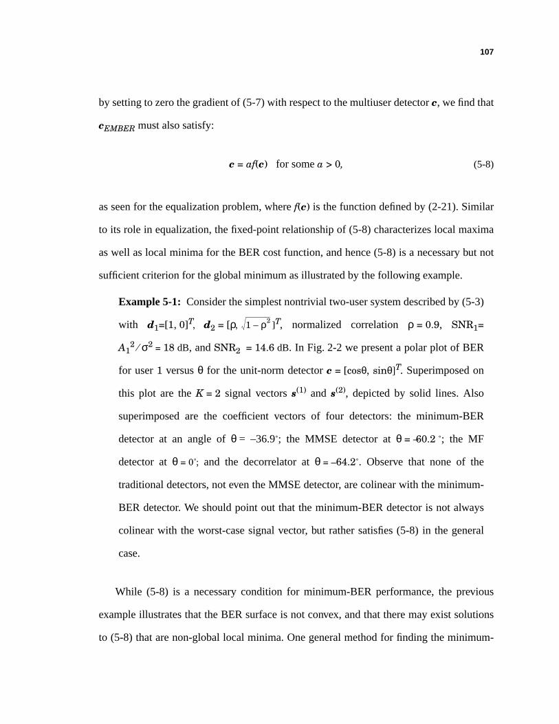
107
by setting to zero the gradient of (5-7) with respect to the multiuser detector c, we find that
cEMBER must also satisfy:
c = af(c) for some a > 0, (5-8)
as seen for the equalization problem, where f(c) is the function defined by (2-21). Similar
to its role in equalization, the fixed-point relationship of (5-8) characterizes local maxima
as well as local minima for the BER cost function, and hence (5-8) is a necessary but not
sufficient criterion for the global minimum as illustrated by the following example.
Example 5-1: Consider the simplest nontrivial two-user system described by (5-3)
with d1=[1, 0]T, d2 = [ρ, ]T, normalized correlation ρ = 0.9, SNR1=
A12 ⁄σ2 = 18 dB, and SNR2 = 14.6 dB. In Fig. 2-2 we present a polar plot of BER
for user 1 versus θ for the unit-norm detector c = [cosθ, sinθ]T. Superimposed on
this plot are the K = 2 signal vectors s(1) and s(2), depicted by solid lines. Also
superimposed are the coefficient vectors of four detectors: the minimum-BER
detector at an angle of θ = –36.9˚; the MMSE detector at θ = –60.2 ˚; the MF
detector at θ = 0˚; and the decorrelator at θ = – 64.2˚. Observe that none of the
traditional detectors, not even the MMSE detector, are colinear with the minimum-
BER detector. We should point out that the minimum-BER detector is not always
colinear with the worst-case signal vector, but rather satisfies (5-8) in the general
case.
While (5-8) is a necessary condition for minimum-BER performance, the previous
example illustrates that the BER surface is not convex, and that there may exist solutions
to (5-8) that are non-global local minima. One general method for finding the minimum-
1 ρ2–
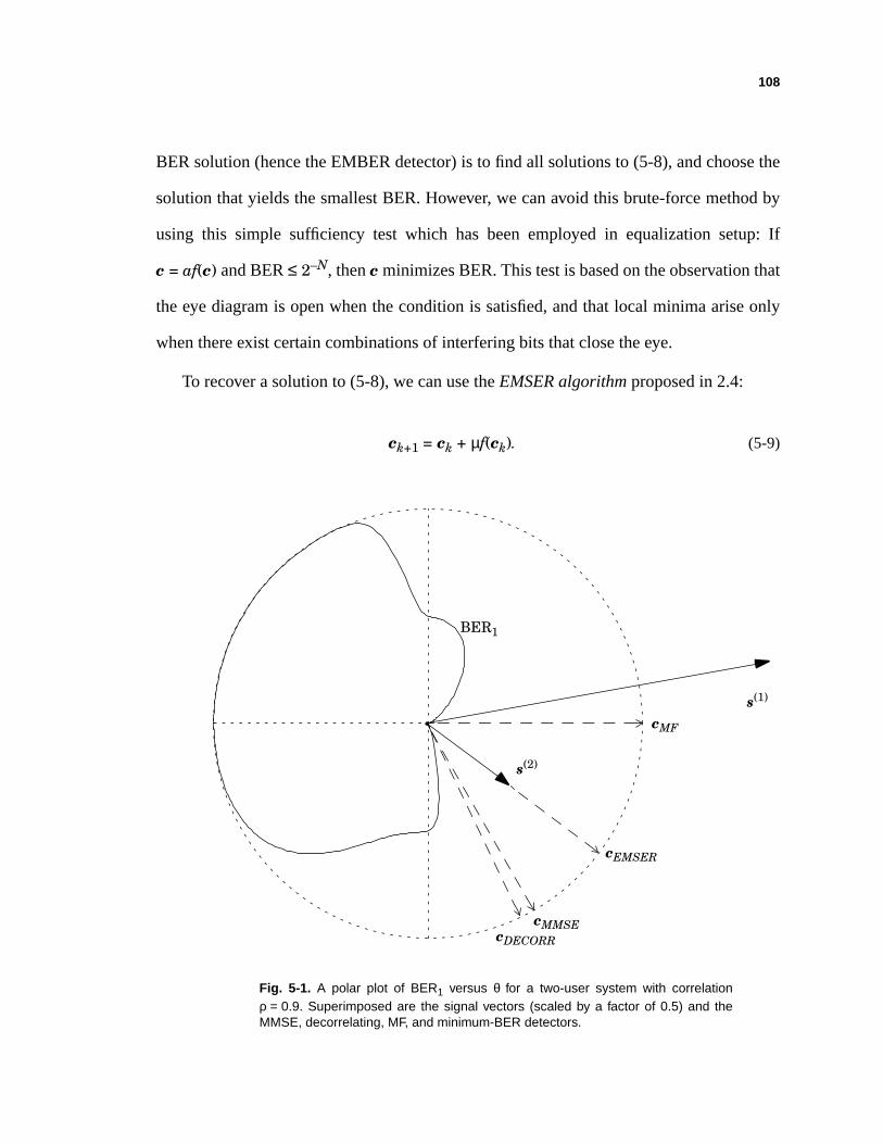
108
BER solution (hence the EMBER detector) is to find all solutions to (5-8), and choose the
solution that yields the smallest BER. However, we can avoid this brute-force method by
using this simple sufficiency test which has been employed in equalization setup: If
c = af(c) and BER ≤ 2– N, then c minimizes BER. This test is based on the observation that
the eye diagram is open when the condition is satisfied, and that local minima arise only
when there exist certain combinations of interfering bits that close the eye.
To recover a solution to (5-8), we can use the EMSER algorithm proposed in 2.4:
ck+1 = ck + µf(ck). (5-9)
Fig. 5-1. A polar plot of BER1 versus θ for a two-user system with correlationρ = 0.9. Superimposed are the signal vectors (scaled by a factor of 0.5) and theMMSE, decorrelating, MF, and minimum-BER detectors.
s(1)
BER1
cEMSER
cMMSE
cMF
s(2)
cDECORR
109
It has been shown that the EMSER algorithm is guaranteed to converge to a solution satis-
fying (5-8). However, convergence of the EMSER algorithm to the global minimum-BER
detector cannot in general be guaranteed.
Similar to the strategy for finding the EMSER equalizer, we use the following strategy
for finding the EMBER linear multiuser detector. First, iterate the EMSER algorithm of
(5-9) until it converges. If the resulting BER ≤ 2– N, stop. Otherwise, initialize the EMSER
algorithm somewhere else and repeat the process. This is an effective strategy when the
initial condition of the EMSER algorithm is chosen carefully and when the SNR is suffi-
ciently large that BER ≤ 2– N is possible.
5.4 APPROXIMATE MINIMUM-BER MULTIUSER DETECTION
Although the EMSER algorithm is useful for finding the minimum-BER detector of
known channels, it is poorly suited for adaptive implementation in time-varying applica-
tions. We now extend the AMBER algorithm of chapter 3 to the multiuser problem.
The numerical algorithm (5-9) can be transformed into a stochastic update equation by
using an error indicator function Iby similar to the error indicator introduced in chapter 3,
where
Iby = (1 – sgn[ yk]), (5-10)
where yk = cTrk is the decision statistic for the kth bit. In other words, Iby = 1 when an
error is made ( ≠ ) and Iby = 0 when no error is made ( = ). Note that
because the multiuser system we are considering is binary, we can effectively treat it as a
2-PAM system where there are no “inner” points in the constellation and thus, simplify the
error indicator in (3-9). With the error indicator and following the previous derivation for
12--- bk
i( )
bki( )
bki( ) bk
i( )bk
i( )
110
approximating the EMSER equalizer algorithm, we transform the EMSER multiuser
detector algorithm of (5-9) using the following equalities:
ck+1 = µf(ck)
≈ ck + µE
= ck + µE
= ck + µE E[Iby| Hbk]E[ Hbk]
= ck + µE[Iby Hbk]
≈ ck + µE[Iby rk] (5-11)
The approximation of (5-11) is valid assuming the effect of noise is insignificant at high
SNR. We can then form a simple stochastic update algorithm by simply removing the
expectation in (5-11):
ck+1 = ck + µIby rk . (5-12)
We refer to this stochastic algorithm as the AMBER algorithm for linear multiuser detec-
tion. The detector is updated only when an error is made. It has an insightful geometric
interpretation. Recall that the noiseless output of the detector when a one is transmitted by
the desired user is the inner product of c with s(j). Most errors occur when this inner
product is small, i.e., when the eye is nearly closed. The AMBER update of (5-12) dictates
that each time an error is made, the detector coefficient vector c takes a small step in space
towards the s(j) vector that resulted in the error. Therefore, the next time the interfering
Qck
Tsck σ
--------------
s
Qbk
i( )ckTHbk
ck σ-----------------------------
bki( )Hxbk
bki( ) bk
i( )
bki( )
bki( )
bki( )
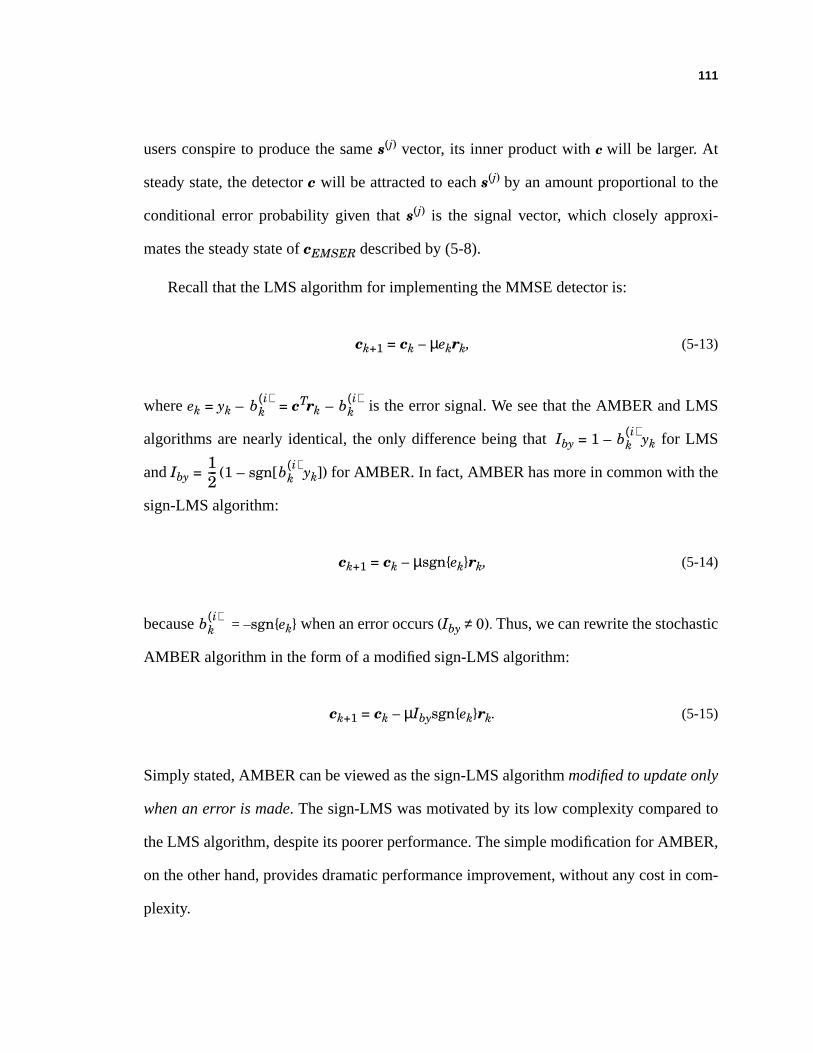
111
users conspire to produce the same s(j) vector, its inner product with c will be larger. At
steady state, the detector c will be attracted to each s(j) by an amount proportional to the
conditional error probability given that s(j) is the signal vector, which closely approxi-
mates the steady state of cEMSER described by (5-8).
Recall that the LMS algorithm for implementing the MMSE detector is:
ck+1 = ck – µekrk, (5-13)
where ek = yk – = cTrk – is the error signal. We see that the AMBER and LMS
algorithms are nearly identical, the only difference being that Iby = 1 – yk for LMS
and Iby = (1 – sgn[ yk]) for AMBER. In fact, AMBER has more in common with the
sign-LMS algorithm:
ck+1 = ck – µsgn{ek}rk, (5-14)
because = –sgn{ek} when an error occurs (Iby ≠ 0). Thus, we can rewrite the stochastic
AMBER algorithm in the form of a modified sign-LMS algorithm:
ck+1 = ck – µIbysgn{ek}rk. (5-15)
Simply stated, AMBER can be viewed as the sign-LMS algorithm modifiedto updateonly
whenan error is made. The sign-LMS was motivated by its low complexity compared to
the LMS algorithm, despite its poorer performance. The simple modification for AMBER,
on the other hand, provides dramatic performance improvement, without any cost in com-
plexity.
bki( ) bk
i( )
bki( )
12--- bk
i( )
bki( )
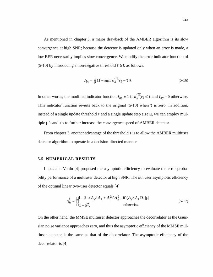
112
As mentionedin chapter3, a major drawback of the AMBER algorithm is its slow
convergenceat high SNR;becausethedetectoris updatedonly whenanerror is made,a
low BER necessarilyimpliesslow convergence.Wemodify theerrorindicatorfunctionof
(5-10) by introducing a non-negative thresholdτ ≥ 0 as follows:
Iby = (1 – sgn[ yk – τ]). (5-16)
In otherwords,themodifiedindicatorfunctionIby = 1 if yk ≤ τ andIby = 0 otherwise.
This indicator function reverts back to the original (5-10) when τ is zero. In addition,
insteadof a singleupdatethresholdτ anda singleupdatestepsizeµ, we canemploy mul-
tiple µ’s andτ’s to further increase the convergence speed of AMBER detector.
Fromchapter3, anotheradvantageof thethresholdτ is to allow theAMBER multiuser
detector algorithm to operate in a decision-directed manner.
5.5 NUMERICAL RESULTS
LupasandVerdú[4] proposedthe asymptoticefficiency to evaluatethe error proba-
bility performanceof amultiuserdetectorathighSNR.Thekth userasymptoticefficiency
of the optimal linear two-user detector equals [4]
= (5-17)
Ontheotherhand,theMMSE multiuserdetectorapproachesthedecorrelatorastheGaus-
siannoisevarianceapproacheszero,andthustheasymptoticefficiency of theMMSE mul-
tiuser detectoris the sameas that of the decorrelator. The asymptoticefficiency of the
decorrelator is [4]
12--- bk
i( )
bki( )
ηkl 1 2 ρ Ai Ak⁄– Ai
2 Ak2,⁄+
1 ρ2,– if Ai Ak⁄( ) ρ≤
otherwise.

113
= 1 – ρ2. (5-18)
Finally, the asymptotic efficiency of the MF detector is [4]
= max2 . (5-19)
Given ρ in a two-user system, we can plot the asymptotic efficiencies of the optimal linear
multiuser detector, the decorrelator, and the MF detector as functions of Ai/Ak. In
Fig. 5-2, we plot user 1 asymptotic efficiencies for ρ = 0.6. The asymptotic efficiencies of
the optimum linear multiuser detector and the decorrelator are the same when A2/A1 is
larger than ρ = 0.6. In addition, the asymptotic efficiencies of the optimum linear multiuser
detector and the MF detector are very close when A2/A1 is small. When the asymptotic
efficiencies of the MF detector and the decorrelator are about the same, the optimum linear
multiuser detector performs significantly better than both of them.
ηkd
ηkm 0,1 ρ
AiAk-------–
Fig. 5-2. Asymptotic efficiencies in two-user case (ρ = 0.6) [4].
0
1
Asy
mpt
otic
Effi
cien
cy (
user
1)
A2/A1
1– ρ2
|ρ| 1/|ρ|
Optimum linear multiuser detectorDecorrelating detectorMF detector

114
With theasymptoticefficienciesof theoptimal linearmultiuserdetectoranddecorre-
lator derived by Lupasand Verdú [4], we can use them as the boundson gain of the
EMBER multiuserdetectorover the MMSE multiuserdetector. We will now compare
BER performancesof the EMBER, AMBER, MMSE, MAME of LupasandVerdú [4],
decorrelator, andMF detectorson a two-usersystemwith d1 = [1, 0]T, d2 = [ρ, ]T
andρ = 0.9. We choosetheinterferencepower of A22 ⁄A1
2 = –4.15 dB sothattheasymp-
totic efficienciesof both the decorrelatorandthe MF detectoraresignificantly lessthan
thatof theoptimumlinearmultiuserdetector, andthuswe expecttheEMBER, AMBER,
andMAME detectorsperformsignificantlybetterthantheMMSE, decorrelating,andMF
detectorsat high SNR. In Fig. 5-3 we comparethe BER performanceof the above six
linearmultiuserdetectors.Observe that theEMBER, AMBER, andMAME detectorsare
indistinguishable,andthatthey outperformtheMMSE detectorby morethan1 dB athigh
SNR and outperform the matched filter and the decorrelator by an even wider margin.
We also considera simple three-usersystemdescribedby (5-3) with d1 = [1, 0.1]T,
d2 = [0.9, 1]T, d3 = [0.1, 1]T, andSNR1 = SNR2 = SNR3 = 20 dB. In Fig. 5-4 weillustrate
the performanceof AMBER, with parametersτ1 = 0.2, τ2 = 0.4, µ1 andµ2 initialized to
0.06 and0.02, andwith µ1 andµ2 cut in half every 200 iterations.AlthoughAMBER can
not improve the BER performancefor user2, it improves BER of users1 and 3 over
MMSE solutions significantly.
For comparisonpurposes,we include in Fig. 5-4 the performanceof the adaptive
detectorof Psaromiligkos et al. [6]. We usedparametersof an = , cn = 0.1n–0.25
(wheren is time),anda thresholdλ = 0.08. Theconvergencerateof this algorithmis com-
parableto thatof AMBER. UnlikeAMBER, however, it requiresknowledgeof all thesig-
nature sequences of users.
1 ρ2–
0.001n( )log
----------------
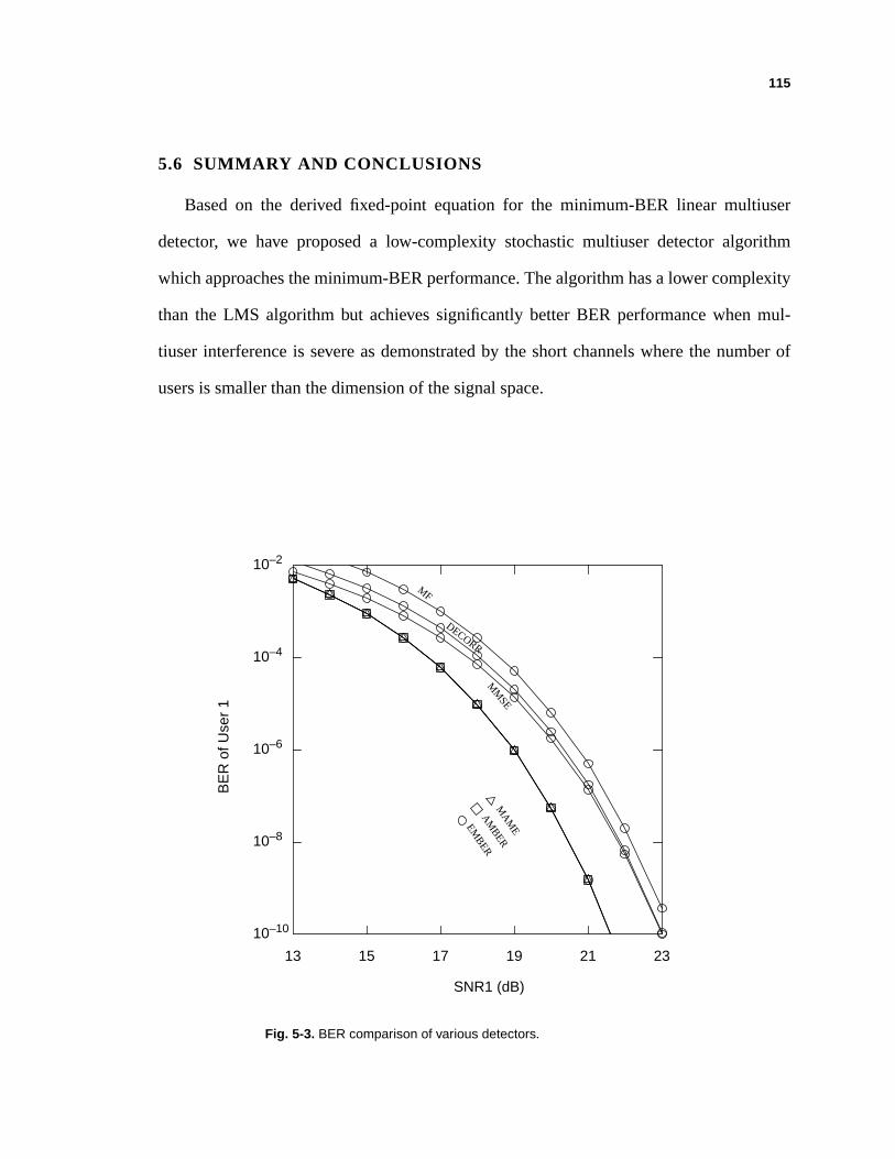
115
5.6 SUMMARY AND CONCLUSIONS
Based on the derived fixed-point equation for the minimum-BER linear multiuser
detector, we have proposed a low-complexity stochastic multiuser detector algorithm
which approaches the minimum-BER performance. The algorithm has a lower complexity
than the LMS algorithm but achieves significantly better BER performance when mul-
tiuser interference is severe as demonstrated by the short channels where the number of
users is smaller than the dimension of the signal space.
SNR1 (dB)
DECORR
MF
MM
SE
EMBER
MA
ME
AM
BER
BE
R o
f Use
r 1
13 15 17 19 21 23
10–10
10–8
10–6
10–4
10–2
Fig. 5-3. BER comparison of various detectors.
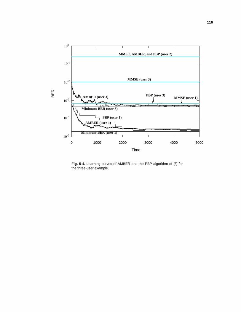
116
0 1000 2000 3000 4000 5000
Time
MMSE, AMBER, and PBP (user 2)
100
10-2
10-1
10-3
10-4
10-5
PBP (user 1)
AMBER (user 1)
PBP (user 3)AMBER (user 3) MMSE (user 1)BE
R
MMSE (user 3)
Minimum-BER (user 1)
Minimum-BER (user 3)
Fig. 5-4. Learning curves of AMBER and the PBP algorithm of [6] forthe three-user example.
117
CHAPTER 6
C O N C L U S I O N S A N DF U T U R E W O R K
6.1 CONCLUSIONS
This thesis has concentrated on the design and adaptation of finite-tap equalizers and
multiuser detectors to minimize error probability. We have proposed low-complexity
equalizer and multiuser detector algorithms for combating ISI and multiuser interference
in the presence of additive Gaussian noise.
In chapter 2, we have derived and investigated the properties of the minimum-SER
equalizer. We have shown that a necessary but not sufficient condition, a fixed-point rela-
tionship, has to be satisfied by the minimum-SER equalizer. We then proposed, based on
the fixed-point relationship, a numerical algorithm to iteratively recover the minimum-
SER equalizer coefficients satisfying the fixed-point relationship. Because satisfaction of
the fixed-point relationship does not guarantee the minimum-SER equalizer, we have also
118
proposed a sufficiency condition for testing the convergence of the numerical algorithm to
the global-SER minimum. The sufficiency condition is based on the mild assumption that
the noise variance is sufficiently small. In addition, we have conjectured that the MMSE
equalizer approaches the minimum-SER equalizer as the number of equalizer taps
approaches infinity.
In chapter 3, we have used another exponential-like function, the Gaussian error func-
tion or Q function, to approximate the fixed-point relationship derived for the minimum-
SER equalizer in chapter 2. Instead of multiple solutions, there is a unique solution to the
approximate fixed-point relationship. We have constructed a numerical algorithm to
recover the unique solution to the approximate relationship. The numerical algorithm
(AMBER) based on the fixed-point relationship yields a low-complexity stochastic equal-
izer algorithm. We have evaluated its error-probability performance and compared it with
the MMSE and the EMSER algorithms. Finally, we have empirically characterized the
FIR channels over which the AMBER and the EMSER equalizers significantly outperform
the MMSE equalizer.
In chapter 4, we have discussed the convergence properties of the AMBER algorithm.
We have first determined the deterministic trajectory of the AMBER algorithm by taking
the expectation of the stochastic update equation. The deterministic trajectory turns out to
be a complicated nonlinear dynamical system. We have then developed some analytical
intuition regarding the dynamical system and have discussed the global convergence prop-
erty of the AMBER algorithm. Although we have not been able to rigorously prove the
global convergence of the algorithm, we have argued that the algorithm is likely to glo-
bally converge. We have then proposed some multi-step variants of AMBER to increase
119
convergencespeed.We also have studied the convergenceperformanceof decision-
directed mode.
In chapter5, we have extendedresultson the minimum-error-probability equalizers
andupdatealgorithmsto multiusersystems.Theconceptsof thesignalvectorsandsignal
conesin a single-userISI channelcanbeextendedin a straightforwardmannerto a mul-
tiuser systemwheremultiuser interferenceis similar to the ISI phenomenon.We have
comparedthe performanceof the minimum-BER multiuserdetectorwith the matched
filter detector, theMMSE detector, thedecorrelator, andtheMAME detectorproposedby
Lupas and Verdú [4].
6.2 FUTURE WORK
6.2.1 MMSE vs. Minimum-SER Equalizers with Infinite Number of Taps
In chapter2, we madea conjecturethat the MMSE equalizerapproachesthe min-
imum-BERequalizerwhenthe numberof equalizertapsapproachesinfinity. Otherthan
somesimulationresults,we currentlydo not have a rigorousmathematicalproof to con-
firm nor a counterexampleto contradictthe claim. A proof or a counterexampleto this
conjecturewould be enlighteningin understandingthe ultimateconnectionbetweenthe
MMSE and the EMSER equalizers.
6.2.2 Global Convergence Proof
In chapter4 we discussedtheglobalconvergencepropertyof theAMBER algorithm.
Ratherthana formalmathematicalproof,wecompletedthetopicwith amixtureof obser-
vationsandanalyticalreasoning.Proving theglobalconvergencepropertyrequiresamore
thorough understanding of this particular nonlinear dynamical system.
120
6.2.3 Multiuser Channels with Memory
In this thesis,we developedandevaluatedminimum-BERresultson single-userISI
channelsand memorylessmultiuserchannels.The theoreticalresultson single userISI
channelsandmemorylessmultiuserchannelscanbeextendednaturallyto multiuserchan-
nelswith memory. However, it will beof practicalinterestto numericallyevaluatetheper-
formance of the AMBER algorithm on multiuser channels with memory.
6.2.4 Blind Equalization and Multiuser Detection
The AMBER algorithmin this thesis,similar to the LMS algorithm,requirescorrect
decisionsin initializing equalizersand multiuser detectors.Recentlythere has beena
surged interestin blind equalization[42] and multiuser detectionresearch[32]. Blind
equalizationandmultiuserdetectionarevaluablewhena trainingsequenceis eithercostly
or impossibleto transmit.Similar to the blind multiuseralgorithm proposedby Honig,
Madhow, and Verdú [43], it will be of practical interestto constructsimple and robust
equalizerandmultiuserdetectoralgorithmsto minimizeerrorprobabilitywithout training
data.
121
R E F E R E N C E S
[1] E. ShamashandK. Yao, “On the StructureandPerformanceof a Linear Deci-sion-FeedbackEqualizerBasedon the Minimum Error Probability Criterion,”International Conference on Communications, pp. 25F1-25F5, 1974.
[2] P. Galko andS. Pasupathy, “Optimal Linear Receiver Filters for Binary DigitalSignals,” International Conference on Communications, pp. 1H.6.1-1H.6.5,1982.
[3] S. Chen,E. Chng,B. Mulgrew, andG. Gibson,“Minimum-BER Linear-Com-biner DFE,” International Conference on Communications, pp. 1173-1177,1996.
[4] R. LupasandS.Verdú,“Linear MultiuserDetectorsfor SynchronousCode-Divi-sionMultiple-AccessChannels,” IEEE Transactions on Information Theory, vol.35, no. 1, pp. 123-136, January 1989.
[5] N. B. Mandayam and B. Aazhang, “Gradient Estimation for Sensitivity Analysisand Adaptive Multiuser InterferenceRejection in Code-Division Multiple-AccessSystems,” IEEE Transactions on Communications, vol. 45, no. 7, pp.848-858, July 1997.
[6] I. N. Psaromiligkos,S.N. Batalama,andD. A. Pados,“AdaptiveMinimum Prob-ability of ErrorLinear-Filter Receiversfor DS-CDMA channels,” Proceedings ofConference on Information Sciences and Systems, pp. 90-94, 1996.
[7] S.U. H. Qureshi,“Adaptive Equalization,” Proceedings of the IEEE, vol. 73,no.9, pp. 1349-1387, September 1985.
[8] R. W. Lucky, “Automatic Equalizationfor Digital Communication,” The BellSystem Technical Journal, vol. 44, pp. 547-588, April 1965.
122
[9] R. W. Lucky, “Techniques for Adaptive Equalization of Digital CommunicationSystems,” The Bell SystemTechnical Journal, vol. 45, pp. 255-286, February1966.
[10] R. W. Lucky, J. Salz, and E. J. Weldon, Principles of Data Communications,McGraw-Hill, 1968.
[11] A. Gersho, “Adaptive Equalization of Highly Dispersive Channels,” The BellSystem Technical Journal, vol. 48, pp. 55-70, January 1969.
[12] J. Proakis and J. Miller, “An Adaptive Receiver for Digital Signaling ThroughChannels with Intersymbol Interference,” IEEE Transactionson InformationTheory, vol. 15, pp. 484-497, 1969.
[13] J. G. Proakis, Digital Communications, Third Edition, McGraw-Hill, 1995.
[14] E. A. Lee and D. G. Messerschmitt, Digital Communication, Second Edition,Kluwer Academic Publishers, 1994.
[15] S. Haykin, Adaptive Filter Theory, Second Edition, Prentice Hall, 1991.
[16] B. Widrow and M. E. Hoff, “Adaptive Switching Circuits,” IRE WESCON, pt. 4,pp. 96-104, August 1960.
[17] B. Widrow and S. D. Stearns, Adaptive Signal Processing, Prentice-Hall, 1985.
[18] S. T. Alexander, Adaptive Signaling Processing, Springer-Verlag, 1986.
[19] C. P. Kwong, “Dual Sign Algorithm for Adaptive Filtering,” IEEE Transactionson Communications, vol. 34, No. 12, December 1986.
[20] R. Sharma, W. Sethares, and J. Bucklew, “Asymptotic Analysis of StochasticGradient-Based Adaptive Filtering Algorithms with General Cost Functions,”IEEE Transactions on Signal Processing, vol. 44, no. 9, September 1996.
[21] S. C. Bang and S. Ann, “A Robust Algorithm for Adaptive FIR Filtering and ItsPerformance Analysis with Additive Contaminated-Gaussian Noise,” IEEETransactionson Circuits and Systems– 1: FundamentalTheoryand Applica-tions, vol. 43, no. 5, May 1996.
[22] G. D. Forney, Jr., “Maximum-likelihood Sequence Estimation of DigitalSequences in the Presence of Intersymbol Interference,” IEEE TransactionsonInformation Theory, vol. 18, no. 3, pp. 363-377, May 1972.
[23] G. D. Forney, Jr., “The Viterbi Algorithm,” Proceedingsof IEEE, vol. 61, no. 3,pp. 268-278, March 1973.
123
[24] D. D. Falconerand F. R. Magee,“Adaptive ChannelMemory TruncationforMaximum-Likelihood SequenceEstimation,” The Bell System Technical Jour-nal, vol. 52, pp. 1541-1562, November 1973.
[25] A. Duel-HallenandC Heegard,“DelayedDecision-FeedbackSequenceEstima-tion,” IEEE Transactions on Communications, vol. 37, no.5,pp. 428-436,May1989.
[26] M. V. EyubogluandS.U. H. Qureshi,“Reduced-StateSequenceEstimationwithSet Partitioning and DecisionFeedback,” IEEE Transactions on Communica-tions, vol. 36, no. 1, January 1988.
[27] M. Austin, “Decision-feedbackEqualizationfor Digital CommunicationoverDispersive Channels,” TechnicalReport437,MIT Lincoln Laboratory, Lexing-ton, Mass, 1967.
[28] P. Monsen, “FeedbackEqualization for Fading Dispersive Channels,” IEEETransactions on Information Theory, vol. 17, pp. 56-64, 1971.
[29] C. A. BelfioreandJ.H. Park, “DecisionFeedbackEqualization,” Proceedings ofthe IEEE, vol. 67, no. 8, August 1979.
[30] J.Salz,“OptimumMean-SquareDecisionFeedbackEqualization,” The Bell Sys-tem Technical Journal, vol. 52, no. 8, pp. 1341-1373, October 1973.
[31] M. S. Mueller andJ. Salz,“A Unified Theoryof Data-AidedEqualization,” TheBell System Technical Journal, vol. 60, no. 11, pp. 2023-2038, November 1981.
[32] J.BarryandA. Batra,“Co-ChannelDemodulationUsingMulti-Input Multi-Out-put Equalization,” CRASP Annual Report: Year Two, July 1996.
[33] S. Verdú,“RecentProgressin Multi-User Detection,” in Advances in Communi-cations and Signal Processing, W. A. PorterandS. C. Kak, Eds.Springer-Ver-lag, New York, 1989.
[34] P. A. VooisandJ.M. Cioffi, “MultichannelSignalProcessingfor Multiple-HeadDigital MagneticRecording,” IEEE Transactions on Magnetics, 30:6,pp. 5100-5114, November 1994.
[35] J. Salz, “Digital TransmissionOver Cross-CoupledLinear Channels,” AT&TTechnical Journal, 64:6, pp. 1147-1158, July-August 1985.
[36] W. Van Etten,“Maximum LikelihoodReceiver for Multiple ChannelTransmis-sion Systems,” IEEE Transactions on Communications, pp. 276-283,February1976.
124
[37] M. K. Varanasiand B. Aazhang,“Near-Optimum Detection in SynchronousCode-Division Multiple-AccessSystems,” IEEE Transactionson Communica-tions, vol. 39, no. 5, pp. 725-736, May 1991.
[38] C.-C.YehandJ. R. Barry, “ApproximateMinimum Bit-Error RateEqualizationfor Binary Signaling,” InternationalConferenceon Communications(ICC ‘97),pp. 1095-1099, 1997.
[39] C.-C.YehandJ. R. Barry, “ApproximateMinimum Bit-Error RateEqualizationfor Binary Signaling,” submittedto IEEE Transactionson Communications,May 1997.
[40] C.-C.YehandJ. R. Barry, “ApproximateBit-Error RateEqualizationfor Pulse-Amplitude and QuadratureAmplitude Modulation,” to apprear, InternationalConference on Communications(ICC ‘98).
[41] C.-C.Yeh,R. P. Lopes,andJ. R. Barry, “ApproximateMinimum Bit-Error RateMultiuser Detection,” submittedto Global CommunicationConference(Globe-Comm ‘98).
[42] S. Haykin,Blind Deconvolution, Prentice Hall, 1994.
[43] M. Honig, U. Madhow, and S. Verdú, “Blind Adaptive Multiuser Detection,”IEEE Transactionson Information Theory, vol. 41, no. 4, pp. 944-960,July1995.