I. GENERAL RELATIVITY – A SUMMARY

A. Pseudo-Riemannian manifolds

Spacetime is a manifold that is continuous and differentiable. This means that we candefine scalars, vectors, 1-forms and in general tensor fields and are able to take derivativesat any point. A differential manifold is an primitive amorphous collection of points (eventsin the case of spacetime). Locally, these points are ordered as points in a Euclidian space.Next, we specify a distance concept by adding a metric g, which contains information abouthow fast clocks proceed and what are the distances between points.

On the surface of the Earth we can determine a metric by drawing small vectors−−→∆P on the

surface. We state that the length of the vector is given by the inner product

−−→∆P ·

−−→∆P ≡

−−→∆P2 = (length of

−−→∆P)2, (1.1)

and use a ruler to determine its value. We now have a definition for the inner vector productfor a small vector with itself. We use linearity to extend this to macroscopic vectors. Next,we can obtain a definition for the inner product of two different vectors by writing

~A · ~B =1

4

[( ~A+ ~B)2 − ( ~A− ~B)2

]. (1.2)

In summary, when one has a distance concept (a ruler on the surface of the Earth), thenone can define an inner product, and from this the metric follows (since it is nothing but

g( ~A, ~B) ≡ ( ~A · ~B) = g( ~B, ~A). The metric tensor is symmetric.). A differentiable manifoldwith a metric as additional structure, is termed a (pseudo-)Riemannian manifold. We now

Figure 1: Left: at each point P on the surface of the Earth a tangent space (in this case a tangentplane) exists; right: the tangent plane is a nearly correct image in the vicinity of the point P.

want to assign a metric to spacetime. To this end we introduce a local Lorentz frame (LLF).We can achieve this by going into freefall at point P . The equivalence principle states thatall effects of gravitation disappear and that we locally obtain the metric of the special theory

1

of relativity (SRT). This is the Minkowski metric. Thus, we can choose at each point Pof the manifold a coordinate system in which the Minkowski metric is valid. While in theSRT this can be a global coordinate system, in general relativity (GR) this is only locallypossible. With this procedure we have now found a definition of distance at each point P :with gµν = ηµν → ds2 = ηµνdx

µdxν . In essence, we practice SRT at each point P and havea measure for lengths of rods and proper times of ideal clocks. In a LLF the metric is givenby ηµν = diag(−1,+1,+1,+1). For a Riemannian manifold all diagonal elements need tobe positive. The signature (the sum of the diagonal elements) of the metric of spacetime is+2, and in our case we refer to the manifold as pseudo-Riemannian.

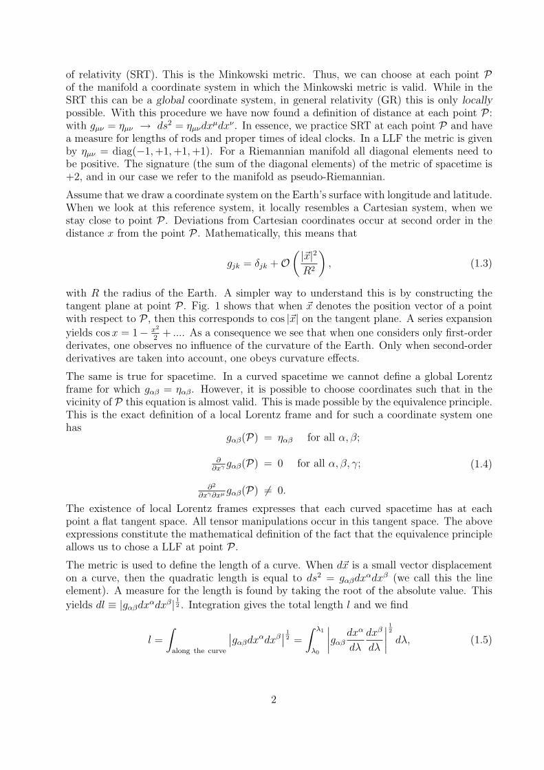
Assume that we draw a coordinate system on the Earth’s surface with longitude and latitude.When we look at this reference system, it locally resembles a Cartesian system, when westay close to point P . Deviations from Cartesian coordinates occur at second order in thedistance x from the point P . Mathematically, this means that

gjk = δjk +O(|~x|2

R2

), (1.3)

with R the radius of the Earth. A simpler way to understand this is by constructing thetangent plane at point P . Fig. 1 shows that when ~x denotes the position vector of a pointwith respect to P , then this corresponds to cos |~x| on the tangent plane. A series expansion

yields cosx = 1− x2

2+ .... As a consequence we see that when one considers only first-order

derivates, one observes no influence of the curvature of the Earth. Only when second-orderderivatives are taken into account, one obeys curvature effects.

The same is true for spacetime. In a curved spacetime we cannot define a global Lorentzframe for which gαβ = ηαβ. However, it is possible to choose coordinates such that in thevicinity of P this equation is almost valid. This is made possible by the equivalence principle.This is the exact definition of a local Lorentz frame and for such a coordinate system onehas

gαβ(P) = ηαβ for all α, β;

∂∂xγ

gαβ(P) = 0 for all α, β, γ;

∂2

∂xγ∂xµgαβ(P) 6= 0.

(1.4)

The existence of local Lorentz frames expresses that each curved spacetime has at eachpoint a flat tangent space. All tensor manipulations occur in this tangent space. The aboveexpressions constitute the mathematical definition of the fact that the equivalence principleallows us to chose a LLF at point P .

The metric is used to define the length of a curve. When d~x is a small vector displacementon a curve, then the quadratic length is equal to ds2 = gαβdx

αdxβ (we call this the lineelement). A measure for the length is found by taking the root of the absolute value. This

yields dl ≡ |gαβdxαdxβ|12 . Integration gives the total length l and we find

l =

∫along the curve

∣∣gαβdxαdxβ∣∣ 12 =

∫ λ1

λ0

∣∣∣∣gαβ dxαdλ dxβ

dλ

∣∣∣∣ 12 dλ, (1.5)

2

where λ is the parameter of the curve. The curve has as end points λ0 and λ1. The tangentvector ~V of the curve has components V α = dxα/dλ and we obtain

l =

∫ λ1

λ0

∣∣∣~V · ~V ∣∣∣ 12 dλ (1.6)

for the length of an arbitrary curve.

When we perform integrations in spacetime it is important to calculate volumes. Withvolume we mean a four-dimensional volume. Suppose that we are in a LLF and havea volume element dx0dx1dx2dx3, with coordinates xα in the local Lorentz metric ηαβ.Transformation theory states that

dx0dx1dx2dx3 =∂(x0, x1, x2, x3)

∂(x0′ , x1′ , x2′ , x3′)dx0′dx1′dx2′dx3′ , (1.7)

where the factor ∂( )/∂( ) is the Jacobian of the transformation of xα′ to xα. One has

∂(x0, x1, x2, x3)

∂(x0′ , x1′ , x2′ , x3′)= det

∂x0

∂x0′∂x0

∂x1′ ...∂x1

∂x0′∂x1

∂x1′ ...... ... ...

= det(Λα

β′

). (1.8)

The calculation of this determinant is rather evolved and it is simpler to realize that in termsof matrices the transformation of the components of the metric is given by the equation(g) = (Λ)(η)(Λ)T , where with ‘T ’ the transpose is implied. Then the determinants obeydet(g) = det(Λ)det(η)det(ΛT ). For each matrix one has det(Λ) = det(ΛT ) and furthermorewe have det(η) = −1. We obtain det(g) = − [det(Λ)]2. We use the notation

g ≡ det(gα′β′) → det(Λαβ′) = (−g)

12 (1.9)

and find

dx0dx1dx2dx3 = det [−(gα′β′)]12 dx0′dx1′dx2′dx3′ = (−g)

12dx0′dx1′dx2′dx3′ . (1.10)

It is important to appreciate the reasoning we followed in order to obtain the above result.We started in a special coordinate system, the LLF, where the Minkowski metric is valid.We then generalized the result to all coordinate systems.

B. Tensors and covariant derivative

Suppose we have a tensor field T( , , ) with rank 3. This field is a function of locationand defines a tensor at each point P . We can expand this tensor in the basis ~eα whichgives the (upper-index) components Tαβγ. In general we have 64 components for spacetime.However, we also can expand the tensor T in the dual basis ~e α and we find

T( , , ) ≡ Tαβγ ~eα ⊗ ~eβ ⊗ ~eγ = T γαβ ~e α ⊗ ~e β ⊗ ~eγ. (1.11)

When we want to calculate the components we use the following theorem:

Tαβγ = T(~e α, ~e β, ~e γ) and T γµν = T(~eµ, ~eν , ~e

γ). (1.12)

3

When we have the components of tensor T in a certain order of upper and lower indices,and we want to know the components with some other order of indices, then the metric canbe used. One has

T γµν = Tαβγgαµgβν and for example also Tαβγ = gαρT βγ

ρ (1.13)

Next, we want to discuss contraction. This is rather complicated to treat in our abstractnotation. Given a tensor R, we always can write it in terms of a vector basis as

R( , , , ) = ~A⊗ ~B ⊗ ~C ⊗ ~D + ... (1.14)

We discuss contraction only for a tensor product of vectors and use linearity to obtain amathematical description for arbitrary tensors. For contraction C13 of the first and thirdindex one has

C13

[~A⊗ ~B ⊗ ~C ⊗ ~D( , , , )

]≡ ( ~A · ~C) ~B ⊗ ~D( , ). (1.15)

We can write the above abstract definition in terms of components and find

~A · ~C = AµCν~eµ · ~eν = AµCνgµν = AµCµ → C13R = Rµβ δµ~B × ~D. (1.16)

In the same way as above, we see that from two vectors ~A and ~B a tensor ~A ⊗ ~B can beconstructed by taking the tensor product, while we can obtain a scalar ~A · ~B by takingthe inner product. The contraction of the tensor product ~A ⊗ ~B again yields a scalar,

C[~A⊗ ~B

]= ~A · ~B.

From now on we will look at expressions such as Rµβ δµ from a different angle. So far we

have viewed these as the components of a tensor; from now on our interpretation is that theindices µ, β, µ and δ label the slots of the abstract tensor R. Thus, Rαβγδ represents theabstract tensor R( , , , ) with as first slot α, second slot β, etc.

The above completes our discussion of tensor algebra. In the following we will discuss tensoranalysis. We do this for a tensor field T( , ) of rank 2, but what we conclude is valid forall tensor fields. The field T is a function of location in the manifold, T(P). We take the

derivative of T along the curve P(λ). At point P the vector ~A tangent to the curve is given

by ~A = dPdλ

= ddλ

. The derivative of T along the curve (so in the direction of vector ~A) isgiven by

∇ ~AT = lim∆λ→0

[T(P(λ+ ∆λ))]‖ −T(P(λ))

∆λ. (1.17)

Notice that the two tensors, T(P(λ+∆λ)) and T(P(λ)), live in two separate tangent spaces.They are almost identical, because ∆λ is small, but nevertheless they constitute differenttangent spaces. We need a way to transport tensor T(P(λ+ ∆λ)) to point P , where we candetermine the derivative, so we can subtract the tensors. What we need is called paralleltransport of T(P(λ+ ∆λ)).

In a curved manifold we do not observe the effects of curvature when we take first-orderderivatives1. Parallel transport then has the same meaning as it does in flat space: the

1 We can always construct a local Lorentz frame which is sufficiently flat for what we intend to do. In that

4

components do not change by the process of transporting. So we have found with Eq. (1.17)an expression for the derivative. The original tensor T( , ) has two slots, and the same istrue for the derivative ∇ ~AT( , ), since according to Eq. (1.17) the derivative is no morethan the difference of two tensors T at different points, and then divided by the distance∆λ.

As a next step we can now introduce the concept of gradient. We notice that the derivative∇ ~AT( , ) is linear in the vector ~A. This means that a rang-3 tensor ∇T( , , ~A) exists, suchthat

∇ ~AT( , ) ≡ ∇T( , , ~A). (1.19)

This is the definition of the gradient of T. The final slot is by convention used as thedifferentiation slot. The gradient of T is a linear function of vectors and has one slot morethat T itself, and furthermore possesses the property that when one inserts ~A in the finalslot, one obtain the derivative of T in the direction of ~A. We define the components of thegradient as

∇T ≡ Tαβ;µ ~eα ⊗ ~eβ ⊗ ~eµ. (1.20)

It is a convention to place the differentiation index below. In addition, notice that one canbring this index up or down, just like any other index. Furthermore, everything else afterthe semicolon corresponds to a gradient. The components of the gradient are in this caseTαβ;µ.

How do we calculate the components of a gradient? The tools for this are the so-calledconnection coefficients2. These coefficients are called this way, because in taking the deriv-ative we have to compare the tensor field at two different tangent spaces. The connectioncoefficients give information about how the basis vectors change between these neighboringtangent spaces. Because we have a basis in point P , we can ask what the derivative of ~eα isin the direction of ~eµ. One has

∇~eµ~eα ≡ Γραµ~eρ. (1.21)

This derivative is itself a vector and we can expand it in our basis at point P where we wantto know the derivative. The expansion coefficients are Γραµ. In the same manner we have

∇~eµ~eρ = −Γρσµ~eσ. (1.22)

system the basis vectors are constant and their derivatives are zero in point P. This constitutes a definition

for the covariant derivative. This definition immediately makes the Christoffel symbols disappear and inthe LLF one has V α;β = V α,β at point P. This is valid for every tensor and for the metric, gαβ;γ = gαβ,γ = 0at point P. Since the equation gαβ;γ = 0 is a tensor equation, it is valid in each basis. Given thatΓµαβ = Γµβα, we find that the metric must obey

Γαµν =12gαβ

(∂

∂xνgβµ +

∂

∂xµgβν −

∂

∂xβgµν

). (1.18)

Thus, while Γαµν = 0 at P in the LLF, this does not hold for its derivatives, because they contain gαβ,γµ.So the Christoffel symbols may be zero at point P when we select a LLF, but in general they differ fromzero in the neighborhood of this point. The difference between a curved and a flat manifold manifestsitself in the derivatives of the Christoffel symbols.

2 These are also known as Christoffel symbols.

5

Notice that we now get a minus sign! The connection coefficients show how basis vectorschange from place to place. So when one wants to find the components of a gradient, forexample Tαβ;γ, then one has to take into account the change of the basis vectors. The tensor

Tαβ itself may be constant and only the basis vectors depend on position. One can showthat

Tαβ;γ = Tαβ,γ + ΓαµγTµβ − ΓµβγT

αµ, where Tαβ,γ = ∂~eγT

αβ =

∂

∂xγTαβ. (1.23)

When we know the metric g, we can calculate the Christoffel symbols, and with them allcovariant derivatives. In this manner we find the equations

V α;β = V α

,β + ΓαµβVµ,

Pα;β = Pα,β − ΓµαβPµ,Tαβ;γ = Tαβ,γ + ΓαµγT

µβ + ΓβµγTαµ.

(1.24)

We introduced the notation Tαβ;µ to underscore the fact that covariant differentiation changes

the rank of a tensor. Another notation which we will use in the rest of these notes is ∇µTαβ.

Note that Tαβ;µ = ∇µTαβ = ∇~eµTαβ. Similarly, we write Tαβ,µ = ∂µT

αβ = ∂Tαβ/∂xµ.

C. Geodesics and curvature

When we draw spherical coordinates on a sphere, and follow two lines, that are perpen-dicular to the equation, in the direction of the North pole, we observe that two initial parallellines meet at a point on the curved surface. The fifth postulate of Euclid does not hold fora curved space: parallel lines can intersect. Another illustration of how curvature manifestsitself is perhaps more effective. It is outlined in Fig. 2. We start in point P with a tangentvector that points in the horizontal direction. We take a small step in the direction of Qand after each step we project the tangent vector again on the local tangent space. This isour method of parallel transport. After completing the trajectory PQRP , we observe thatthe final vector is not parallel to the initial vector. This does not occur in a flat space andis an effect of the curvature of the sphere. The consequence is that on a sphere we cannotdefine vector fields that are parallel in a global sense. The result of the process of paralleltransport depends on the path chosen and on the size of the loop.

In order to find a mathematical description, we interpret the interval PQ in Fig. 2 as acurve, and view λ as the parameter of this curve. The vector field ~V is defined at each pointof the curve. The vector ~U = d~x/dλ is the vector tangent to the curve. Parallel transport

means that in a local inertial coordinate frame at point P the components of ~V must beconstant along the curve. One has

dV α

dλ= Uβ∂βV

α = Uβ∇βVα = 0 at point P . (1.25)

The first equality corresponds to the definition of the derivative of a function (in this caseV α) along the curve, the second equality arises from the fact that Γαµν = 0 at point P inthese coordinates. The third equality is a frame-independent expression that is valid in any

6

Figure 2: Parallel transport of a vector ~V around a triangular path PQRP on the surface of asphere. By transporting ~V along the loop PQRP the final vector will be rotated with respect tothe initial vector. The angle of rotation depends on the size of the loop, the path chosen, and thecurvature of the manifold.

basis. We take this as the coordinate system independent definition of the parallel transportof ~V along ~U . A vector ~V is parallel transported along a curve with parameter λ when

Uβ∇βVα = 0 ↔ d

dλ~V = ∇~U

~V = 0. (1.26)

The last step makes use of the notation for the directional derivative along ~U .

The most important curves in a curved spacetime are the geodesics. Geodesics are lines thatare drawn as straight as possible, with as condition that the tangent vectors ~U of these linesare parallel transported. For a geodesic one has

∇~U~U = 0. (1.27)

Notice that in a LLF these lines are indeed straight. For the components one has

Uβ∇βUα = Uβ∂βU

α + ΓαµβUµUβ = 0. (1.28)

When λ is the parameter of the curve, then Uα = dxα/dλ and Uβ∂/∂xβ = d/dλ. We thenfind

d

dλ

(dxα

dλ

)+ Γαµβ

dxµ

dλ

dxβ

dλ= 0. (1.29)

Since the Christoffel symbols are known functions of the coordinates xα, this is a set ofnon-linear second-order differential equations for xα(λ). These have unique solutions whenthe initial conditions at λ = λ0 are given: xα0 = xα(λ0) and Uα

0 = (dxα/dλ)λ0 . Thus, bystating the initial position (xα0 ) and velocity (Uα

0 ), we obtain a unique geodesic.

7

By changing the parameter λ, we mathematically change the curve (but not the path).When λ is a parameter of the geodesic, and we define a new parameter φ = aλ + b, with aand b constants, that do not depend on position on the curve, then we have for φ also

d2xα

dφ2+ Γαµβ

dxµ

dφ

dxβ

dφ= 0. (1.30)

Only linear transformations of λ yield new parameters that satisfy the geodesic equation.We call the parameters λ and φ affine parameters. Finally, we remark that a geodesic is alsoa curve with extremal length (minimum length between two points). Consequently, we canderive the expression for a geodesic also from the Euler-Lagrange equations. In that casewe start from Eq. (1.5). We can also show that the length ds along the curve is an affineparameter.

D. Curvature and the Riemann tensor

In Fig. 3 we show two vector fields ~A and ~B. The vectors are sufficiently small thatthe curvature of the manifold plays no role in the area where this diagram is drawn. Thuswe can assume that the vectors live on the surface instead in the tangent space. In orderto calculate the commutator [ ~A, ~B], we use a local orthonormal coordinate system. Sincewe can interpret a vector as a directional derivative, expression Aα∂Bβ/∂xα represents the

amount by which the vector ~B changes when it is transported along ~A (this is represented bythe short dashed line in the upper right corner in Fig 3). In the same manner Bα∂Aβ/∂xα

Figure 3: The commutator [ ~A, ~B] of two vector fields. We assume that the vectors are small, suchthat curvature allows them to live in the manifold.

represents the change when ~A is transported along ~B (this corresponds to the other short-dashed line). For the components of the commutator in a coordinate system one has

[ ~A, ~B] =

[Aα

∂

∂xα, Bβ ∂

∂xβ

]=

(Aα

∂Bβ

∂xα−Bα∂A

β

∂xα

)∂

∂xβ. (1.31)

8

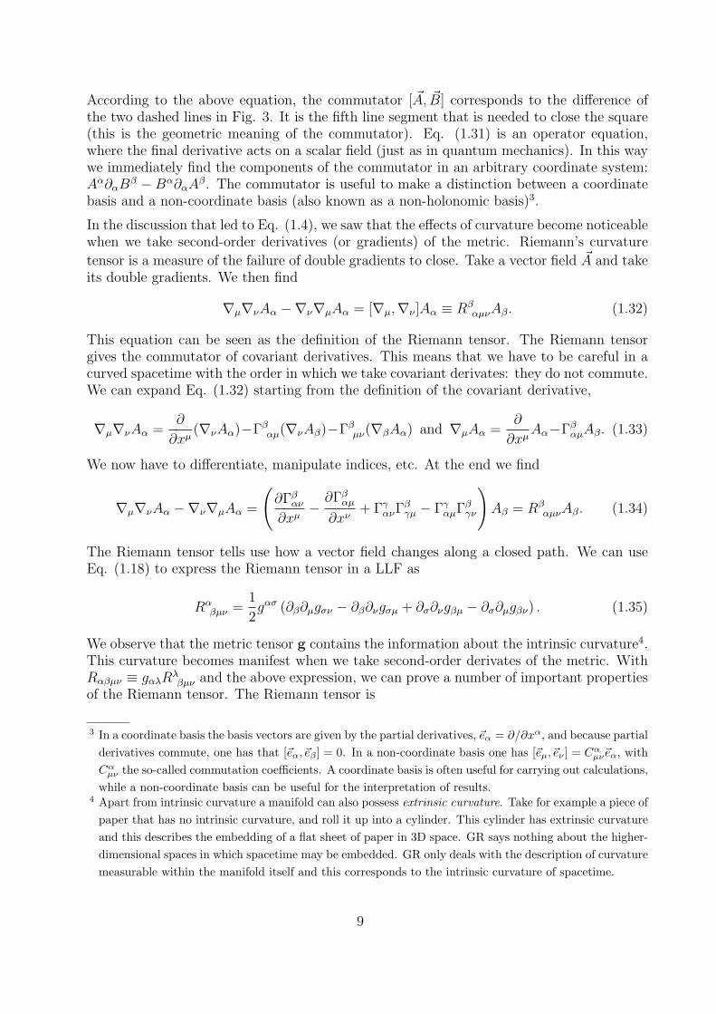
According to the above equation, the commutator [ ~A, ~B] corresponds to the difference ofthe two dashed lines in Fig. 3. It is the fifth line segment that is needed to close the square(this is the geometric meaning of the commutator). Eq. (1.31) is an operator equation,where the final derivative acts on a scalar field (just as in quantum mechanics). In this waywe immediately find the components of the commutator in an arbitrary coordinate system:Aα∂αB

β − Bα∂αAβ. The commutator is useful to make a distinction between a coordinate

basis and a non-coordinate basis (also known as a non-holonomic basis)3.

In the discussion that led to Eq. (1.4), we saw that the effects of curvature become noticeablewhen we take second-order derivatives (or gradients) of the metric. Riemann’s curvature

tensor is a measure of the failure of double gradients to close. Take a vector field ~A and takeits double gradients. We then find

∇µ∇νAα −∇ν∇µAα = [∇µ,∇ν ]Aα ≡ RβαµνAβ. (1.32)

This equation can be seen as the definition of the Riemann tensor. The Riemann tensorgives the commutator of covariant derivatives. This means that we have to be careful in acurved spacetime with the order in which we take covariant derivates: they do not commute.We can expand Eq. (1.32) starting from the definition of the covariant derivative,

∇µ∇νAα =∂

∂xµ(∇νAα)−Γβαµ(∇νAβ)−Γβµν(∇βAα) and ∇µAα =

∂

∂xµAα−ΓβαµAβ. (1.33)

We now have to differentiate, manipulate indices, etc. At the end we find

∇µ∇νAα −∇ν∇µAα =

(∂Γβαν∂xµ

−∂Γβαµ∂xν

+ ΓγανΓβγµ − ΓγαµΓβγν

)Aβ = Rβ

αµνAβ. (1.34)

The Riemann tensor tells use how a vector field changes along a closed path. We can useEq. (1.18) to express the Riemann tensor in a LLF as

Rαβµν =

1

2gασ (∂β∂µgσν − ∂β∂νgσµ + ∂σ∂νgβµ − ∂σ∂µgβν) . (1.35)

We observe that the metric tensor g contains the information about the intrinsic curvature4.This curvature becomes manifest when we take second-order derivates of the metric. WithRαβµν ≡ gαλR

λβµν and the above expression, we can prove a number of important properties

of the Riemann tensor. The Riemann tensor is

3 In a coordinate basis the basis vectors are given by the partial derivatives, ~eα = ∂/∂xα, and because partialderivatives commute, one has that [~eα, ~eβ ] = 0. In a non-coordinate basis one has [~eµ, ~eν ] = Cαµν~eα, withCαµν the so-called commutation coefficients. A coordinate basis is often useful for carrying out calculations,while a non-coordinate basis can be useful for the interpretation of results.

4 Apart from intrinsic curvature a manifold can also possess extrinsic curvature. Take for example a piece ofpaper that has no intrinsic curvature, and roll it up into a cylinder. This cylinder has extrinsic curvatureand this describes the embedding of a flat sheet of paper in 3D space. GR says nothing about the higher-dimensional spaces in which spacetime may be embedded. GR only deals with the description of curvaturemeasurable within the manifold itself and this corresponds to the intrinsic curvature of spacetime.

9

• Antisymmetric in the last two indices. One has

R( , , ~A, ~B) = −R( , , ~B, ~A) or Rµναβ = −Rµνβα. (1.36)

• Antisymmetric in the first two indices. One has

R( ~A, ~B, , ) = −R( ~B, ~A, , ) or Rµναβ = −Rνµαβ. (1.37)

• The tensor is symmetric under exchange of the first and second pair of indices,

R( ~A, ~B, ~C, ~D) = R(~C, ~D, ~A, ~B) or Rµναβ = Rαβµν . (1.38)

• One has the so-called Bianchi identities,

∇µRαβγδ +∇γRαβδµ +∇δRαβµγ = 0. (1.39)

The above symmetries reduce the 4× 4× 4× 4 = 256 components of the Riemann tensor to20.

The Ricci curvature tensor (Ricci tensor) is defined as the contraction of the Riemann tensor.One has

Rαβ ≡ Rµαµβ. (1.40)

For example, in the case of the surface of the Earth this tensor also contains informationabout the curvature, but as the Riemann tensor integrated over angles. Furthermore, onecan show that the Ricci tensor is symmetric. Finally, we have the scalar curvature, the Riccicurvature, defined by

R = Rαα. (1.41)

We have now defined the tensors we need for the description of phenomena in GR. Animpressive mathematical apparatus has been created and we are going to put this to firstuse in order to pose the field equations (the so-called Einstein equations) of GR. We will tryto make this plausible through an analogy with the Newtonian description.

E. Newtonian description of tidal forces

We try to find a measure of the curvature of spacetime. We start our experiment bydropping a test particle. We decide as observer5 to go in freefall along with the particle(LLF) and observe that the particle moves along a straight line in spacetime (only in the timedirection). There is nothing in the motion of a single particle that betrays curvature. Indeed,in a free-falling coordinate system, the particle is at rest. A single particle is insufficient todiscover effects of curvature.

Next, we drop two particles. We will study the tidal force on Earth from the perspective ofobservers that free-fall (LLF) together with the particles. Such observers fall in a straight linetowards the center of the Earth. Fig. 4 outlines the situation for two free-falling particles

5 For simplicity we assume that as observer we do not influence the process. Most importantly, we assumethat we do not introduce gravitational forces or cause curvature of our own.

10

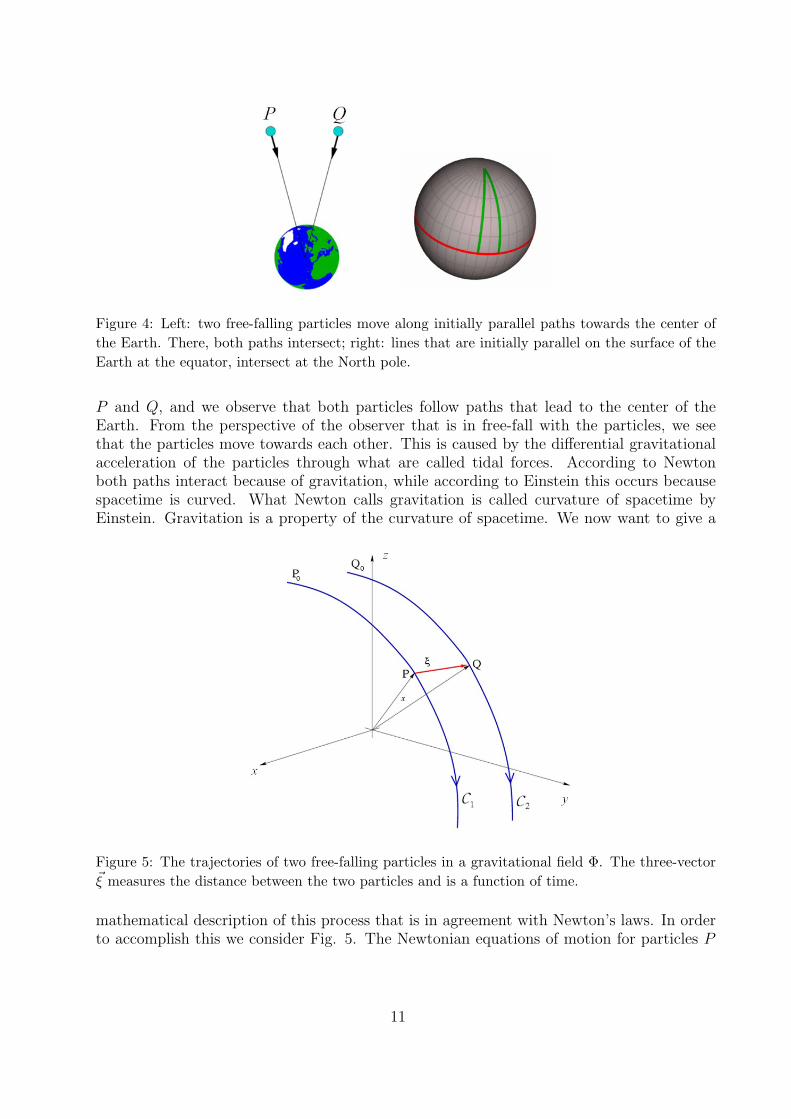
Figure 4: Left: two free-falling particles move along initially parallel paths towards the center ofthe Earth. There, both paths intersect; right: lines that are initially parallel on the surface of theEarth at the equator, intersect at the North pole.

P and Q, and we observe that both particles follow paths that lead to the center of theEarth. From the perspective of the observer that is in free-fall with the particles, we seethat the particles move towards each other. This is caused by the differential gravitationalacceleration of the particles through what are called tidal forces. According to Newtonboth paths interact because of gravitation, while according to Einstein this occurs becausespacetime is curved. What Newton calls gravitation is called curvature of spacetime byEinstein. Gravitation is a property of the curvature of spacetime. We now want to give a

Figure 5: The trajectories of two free-falling particles in a gravitational field Φ. The three-vector~ξ measures the distance between the two particles and is a function of time.

mathematical description of this process that is in agreement with Newton’s laws. In orderto accomplish this we consider Fig. 5. The Newtonian equations of motion for particles P

11

and Q are (d2xjdt2

)(P )

= −(∂Φ

∂xj

)(P )

and

(d2xjdt2

)(Q)

= −(∂Φ

∂xj

)(Q)

, (1.42)

with Φ the gravitational potential. We define ~ξ as the separation between both particles.

For parallel trajectories one has d~ξdt

= 0. With ~ξ = (xj)(P ) − (xj)(Q) we find from a Taylor

expansion that to leading order in the small separation ~ξ

d2ξjdt2

= −(

∂2Φ

∂xj∂xk

)ξk = −Ejkξk → Ejk =

(∂2Φ

∂xj∂xk

), (1.43)

with E the gravitational tidal tensor. Notice that the metric for the 3D Euclidian space isgiven by δjk = diag(1, 1, 1) and that there is no difference between lower and upper indices.Eq. (1.43) is called the equation of Newtonian geodesic deviation.

According to Newton, particles moves towards each other and we write

d2~ξ

dt2= −E( , ~ξ) (1.44)

in abstract notation. It is interesting that the field equation of Newtonian gravitation,

∇2Φ = 4πGρ, (1.45)

can be expressed in terms of second derivatives of Φ, which describe the tidal accelerationsin Eq. (1.43). There is an analogous connection in GR.

F. The Einstein equations

We now arrive at the heart of GR, the field equations. We will try to make the fieldequations plausible in manner that summarizes all previous statements. In Fig. 6 (leftdiagram) we start with a discussion of the motion of a particle along a worldline. Thisworldline is parameterized with proper time τ on a clock that is carried by the particle. Wecan denote the position of the particle at a point of the worldline with P(τ). The velocity

Figure 6: Left: the worldline of a particle is a curve xα(τ) that can be parameterized with theproper time τ of the particle. The velocity ~U is the vector tangent to the curve. Right: we createa coordinate system xα. The velocity ~U now has components Uα = dxα/dτ .

12

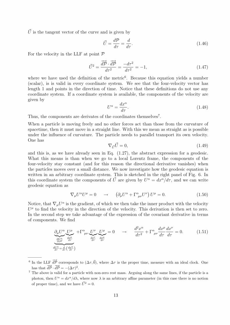
~U is the tangent vector of the curve and is given by

~U =dPdτ

=d

dτ. (1.46)

For the velocity in the LLF at point P

~U2 =

−→dP ·

−→dP

dτ 2=−dτ 2

dτ 2= −1, (1.47)

where we have used the definition of the metric6. Because this equation yields a number(scalar), is is valid in every coordinate system. We see that the four-velocity vector haslength 1 and points in the direction of time. Notice that these definitions do not use anycoordinate system. If a coordinate system is available, the components of the velocity aregiven by

Uα =dxα

dτ. (1.48)

Thus, the components are derivates of the coordinates themselves7.

When a particle is moving freely and no other forces act than those from the curvature ofspacetime, then it must move in a straight line. With this we mean as straight as is possibleunder the influence of curvature. The particle needs to parallel transport its own velocity.One has

∇~U~U = 0, (1.49)

and this is, as we have already seen in Eq. (1.27), the abstract expression for a geodesic.What this means is than when we go to a local Lorentz frame, the components of thefour-velocity stay constant (and for this reason the directional derivative vanishes) whenthe particles moves over a small distance. We now investigate how the geodesic equation iswritten in an arbitrary coordinate system. This is sketched in the right panel of Fig. 6. Inthis coordinate system the components of ~U are given by Uα = dxα/dτ , and we can writegeodesic equation as

∇µUαUµ = 0 →

(∂µU

α + ΓαµνUν)Uµ = 0. (1.50)

Notice, that ∇µUα is the gradient, of which we then take the inner product with the velocity

Uµ to find the velocity in the direction of the velocity. This derivation is then set to zero.In the second step we take advantage of the expression of the covariant derivative in termsof components. We find

∂µUα︸ ︷︷ ︸

∂Uα

∂xµ

Uµ︸︷︷︸dxµ

dτ︸ ︷︷ ︸dUα

dτ= ddτ ( dxαdτ )

+Γαµν Uν︸︷︷︸

dxν

dτ

Uµ︸︷︷︸dxµ

dτ

= 0 → d2xα

dτ 2+ Γαµν

dxµ

dτ

dxν

dτ= 0. (1.51)

6 In the LLF−→dP corresponds to (∆τ,~0), where ∆τ is the proper time, measure with an ideal clock. One

has that−→dP ·

−→dP = −(∆τ)2.

7 The above is valid for a particle with non-zero rest mass. Arguing along the same lines, if the particle is aphoton, then Uα = dxα/dλ, where now λ is an arbitrary affine parameter (in this case there is no notionof proper time), and we have ~U2 = 0.

13

It is important to realize that we have started from the abstract tensor Eq. (1.49) for ageodesic. After defining an arbitrary coordinate system we have written this equation interms or coordinates and the result is expression (1.51). This expression yields four ordinarysecond-order differential equations for the coordinates x0(τ), x1(τ), x2(τ) and x3(τ). Theseequation are coupled through the connection coefficients. Because we are dealing withsecond-order differential equations, we need two initial conditions, for example at time τ = 0the values of both xα(τ = 0) and dxα

dτ(τ = 0) = Uα(0). After this the worldline of a free

particle (geodesic) is fully determined.

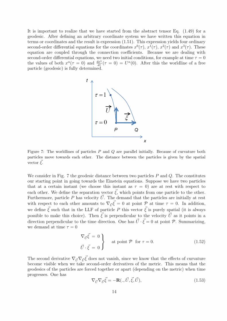
Figure 7: The worldlines of particles P and Q are parallel initially. Because of curvature bothparticles move towards each other. The distance between the particles is given by the spatialvector ~ξ.

We consider in Fig. 7 the geodesic distance between two particles P and Q. The constitutesour starting point in going towards the Einstein equations. Suppose we have two particlesthat at a certain instant (we choose this instant as τ = 0) are at rest with respect to

each other. We define the separation vector ~ξ, which points from one particle to the other.Furthermore, particle P has velocity ~U . The demand that the particles are initially at rest

with respect to each other amounts to ∇~U~ξ = 0 at point P at time τ = 0. In addition,

we define ~ξ such that in the LLF of particle P this vector ~ξ is purely spatial (it is always

possible to make this choice). Then ~ξ is perpendicular to the velocity ~U as it points in a

direction perpendicular to the time direction. One has ~U · ~ξ = 0 at point P . Summarizing,we demand at time τ = 0

∇~U~ξ = 0

~U · ~ξ = 0

at point P for τ = 0. (1.52)

The second derivative ∇~U∇~U~ξ does not vanish, since we know that the effects of curvature

become visible when we take second-order derivatives of the metric. This means that thegeodesics of the particles are forced together or apart (depending on the metric) when timeprogresses. One has

∇~U∇~U~ξ = −R( , ~U, ~ξ, ~U), (1.53)

14

with R the curvature tensor. This equation describes how two initially parallel geodesicsincreasingly deviate as time progresses, as a result of curvature. The expression follows from

Eqs. (1.24) and (1.32). The second derivative ∇~U∇~U~ξ describes the relative acceleration of

the particles.

In the LLF of particle P at time τ = 0 one has U0 = 1 and U i = 0. Therefore, we expect

(∇~U∇~U~ξ)j =

∂2~ξj

∂t2= −Rj

αβγUαξβUγ = −Rj

0k0ξk, (1.54)

since the velocity ~U only has a non-vanishing time component in the LLF of particle P ,

while the separation vector ~ξ only has spacelike components k = 1, 2, 3. In the LLF theequation for the geodesic deviation takes the form

∂2ξj

∂t2= −Rj

0k0ξk, (1.55)

while in Newtonian mechanics we have found (see Eq. (1.43)) that

∂2ξj

∂t2= −Ejkξk. (1.56)

In a LLF the spatial part of the metric is Cartesian (δij = diag(1, 1, 1)) and the position ofthe indices is irrelevant. Comparing both expressions yields

Rj0k0 = Ejk =∂2Φ

∂xjxk. (1.57)

We can identify part of the curvature tensor with derivatives of the Newtonian gravitationalpotential. According to Newton one has

∇2Φ = 4πGρ → ∂j∂kΦ δjk = Ejkδjk = E jj, (1.58)

and we find for the trace of the gravitational tidal tensor E jj = 4πGρ. In analogy one mightexpect that in GR one has

Rj0j0 = 4πGρ ? (1.59)

as a first guess.

However, there is a fundamental problem with Eq. (1.59). It should be an expressionthat does not depend on the choice of coordinate system. Indeed, we have constructedthe equation in a special system: the LLF. What we need to do is find a relation betweentensors. In this context we note that in the LLF one has R0000 = 0 en R0

000 = 0 because ofantisymmetry. Thus one has Rj

0j0 = 4πGρ→ Rµ0µ0 = 4πGρ. We are still in the LLF (note

that also R00 = 4πGρ with R00 the Ricci tensor).

There is another difficulty with Eq. (1.59): at the left of the equal sign we have two indices(which both happen to be 0) while at the right there are none. Thus, one might expect that

Rαβ = 4πGTαβ ? (1.60)

Here, Tαβ represents the energy stress tensor, with T00 = ρ (and this often the dominatingterm in the LLF). Einstein made this guess already in 1912, but it is incorrect! These

15

equations have built-in inconsistencies. It is important to understand what is wrong, and itcan be explained as follows. Consider the Riemann tensor. Schematically,

Rδαβγ ≈ ∂δ∂γgαβ + non-linear terms. (1.61)

When we contract the first and third index, we obtain

Rαγ ≈ ∂β∂γgαβ + non-linear terms. (1.62)

We see that the proposed equations (1.60) constitute a set of 10 partial differential equationsfor the 10 components of the metric gαβ (since the metric is symmetric in α and β). Alsothe Ricci tensor is symmetric. This may all appear fine, but we are at liberty to choosethe coordinate system where we are going to work out the equations. We have the freedomto choose x0(P), x1(P), x2(P) and x3(P). We can use this freedom to set 4 of the 10components of gαβ, viewed as functions of the coordinates, equal to whatever we like (whilepreserving the signature), for example g00 = −1, g01 = g02 = g03 = 0. However, ourequations (1.60) do not allow this, as we would have 10 partial differential equations for 6unknowns. What we need are 6 equations for 6 unknowns.

Before we proceed with our quest for the Einstein equations, two remarks are in order. Thefirst remark has to do with the Bianchi identities. Thanks to these identities∇µRαβγδ+... = 0it follows that when we define the Einstein tensor

Gαβ ≡ Rαβ −1

2Rgαβ, (1.63)

with Rαβ the Ricci tensor and R the scalar curvature, then the Bianchi identities ensurethat the divergence of the Einstein tensor is equal to zero,

∇βGαβ = 0. (1.64)

The second remark pertains to the well-known conservation laws for energy and momentum.In a LLF one has

∂βTαβ = 0 →

∂T 00

∂t+ ∂T 0j

∂xj= 0,

∂T j0

∂t+ ∂T jk

∂xk= 0.

(1.65)

Note that ∂T 0j

∂xjis the spatial divergence and conservation of energy states ∂ρ/∂t+ div ~J = 0,

with ~J the mass-energy flux. In the same manner ∂T j0

∂trepresents the momentum density

and ∂T jk

∂xkthe momentum flux. Since we only take first derivatives, what is valid in flat space

in the LLF is also valid for curved spacetime. In this manner we deduce the tensor equation

∇βTαβ = 0. (1.66)

It seems reasonable to assume that Nature has chosen

Gαβ =8πG

c4Tαβ. (1.67)

These are the Einstein equations. The proportionality factor (8πG/c4) can be found bytaking the Newtonian limit. Before we impose the Einstein equations, we already know that

∇βGαβ = 0 =

8πG

c4∇βT

αβ. (1.68)

16

These are 4 equations and they are in fact the derivatives of the Einstein equations. These4 identities (the divergences of Gαβ and Tαβ vanish) are already satisfied. This puts 4constrains on the Einstein equations (also called the field equations) and the field equationsonly yield 6 new pieces of information. This is exactly what we need.

G. Weak gravitational fields and the Newtonian limit

It is clear that GR describes gravitation in terms of curvature of spacetime and reduces toSRT for local Lorentz frames. However, it is important to explicitly check that the descrip-tion reduces to the Newtonian treatment when we select the correct boundary conditions.

Without gravitation, spacetime possesses the Minkowski metric ηµν . Therefore, weak grav-itational fields only cause small curvatures of spacetime. We assume that coordinates exist,such that the metric takes the following form,

gµν = ηµν + hµν with |hµν | 1. (1.69)

Furthermore, we assume that in this coordinate system the metric is stationary, and that wehave ∂0gµν = 0. The worldline of a free-falling particle is given by the geodesic expression

d2xµ

dτ 2+ Γµνσ

dxν

dτ

dxσ

dτ= 0. (1.70)

We assume that the particle is moving slowly (non-relativistically), such that for the com-ponents of the three-velocity one has dxi/dt c (i = 1, 2, 3), with t defined via x0 = ct. Inthis manner we demand for i = 1, 2, 3

dxi

dτ dx0

dτ. (1.71)

We can neglect the three-velocity and find

d2xµ

dτ 2+ Γµ00c

2

(dt

dτ

)2

= 0. (1.72)

We use Eq. (1.18) and find

Γµ00 =1

2gκµ(∂0g0κ + ∂0g0κ − ∂κg00) = −1

2gκµ∂κg00 = −1

2ηκµ∂κh00, (1.73)

where we used equation (1.69). The last equality is valid to first order in hµν . Since weassumed a stationary metric,

Γ000 = 0 and Γi00 =

1

2δij∂jh00 with i = 1, 2, 3. (1.74)

Inserting this in Eq. (1.72) yields

d2t

dτ 2= 0 and

d2~x

dτ 2= −1

2c2

(dt

dτ

)2

∇h00. (1.75)

17

The first equation states that dt/dτ = constant, and using this we can combine the twoexpressions. This gives the following equation of motion for the particle,

d2~x

dt2= −1

2c2∇h00. (1.76)

When we compare this equation with the Newtonian expression for the motion of a particlein a gravitational field (see Eq. (1.42)), we conclude that the expressions are identical whenwe identify h00 = 2Φ/c2. We find that for a slowly moving particle, GR is equivalent to theNewtonian description when the metric is given by

g00 = 1 + h00 =

(1 +

2Φ

c2

). (1.77)

We can estimate this correction to the Minkowski metric, since Φc2

= −GMc2r

and find −10−9

at the surface of the earth, −10−6 at the surface of the sun, and −10−4 at the surface of awhite dwarf. We conclude that the weak-field limit is an excellent approximation.

Thus, Eq. (1.77) shows that spacetime curvature in general causes the time coordinate t todiffer from the proper time. Consider a clock at rest at a certain point in our coordinatesystem, so that dxi/dt = 0. The proper time interval dτ between two ticks of this clock isgiven by c2dτ 2 = gµνdx

µdxν = g00c2dt2, and we find

dτ =

(1 +

2Φ

c2

) 12

dt. (1.78)

This gives the interval in proper time dτ that corresponds to an interval dt in coordinate timefor a stationary observer in the vicinity of a massive object, in a region with gravitationalpotential Φ. Since Φ is negative, this proper time interval is shorter than the correspondinginterval for a stationary observer at large distance to the object, where Φ → 0 and thusdτ = dt. The spacetime interval is given by

Figure 8: Trajectories of a ball and a bullet in space. Seen in a laboratory the two trajectorieshave different curvature.

ds2 = −(

1 +2Φ

c2

)(cdt)2 + dx2 + dy2 + dz2. (1.79)

18

This expression describes a geometry of spacetime where particles move on geodesics inthe same manner as those of particles in a flat space where the Newtonian force of grav-ity is active. We have found a curved spacetime picture for Newtonian gravitation. Thecurvature is solely in the time direction. Curvature in time is nothing but the gravitationalredshift: time proceeds with different speed at different locations, thus time is curved. Thisgravitational redshift fully determines the trajectories of particles in a gravitational field.Newtonian gravitation corresponds solely to a curvature of time.

Perhaps the above is counter-intuitive, since nothing seems more natural than the idea thatgravitation is a manifestation of the curvature of space. Look for example at the trajectoriesof two objects in space, as shown in Fig. 8. One of the objects is a ball that is moving with arelatively low speed of 5 m/s; it reaches a height of 5 m. The other object is the bullet froma gun. This bullet moves at a much higher speed (500 m/s). When we study the figure, itseems that the orbit of the ball is more strongly curved than that of the bullet.

However, we should not look at the curvature of space, but at the curvature of spacetime.To accomplish this we redraw the trajectories in Fig. 9, but now in Minkowski spacetime.We observe that the trajectories of ball and bullet have a similar curvature in spacetime.However, in reality none of the trajectories has any curvature! They appear curved because

Figure 9: Trajectories of a ball and a bullet is spacetime. Seen in a laboratory both trajectorieshave the same curvature. We compare the orbital length to the arc length of the circle: (radius)= (horizontal distance)2 / 8(height).

we have forgotten that the spacetime in which they are drawn is itself curved. The curvatureof spacetime is exactly such that the orbits themselves are completely straight: they aregeodesics.

19

H. Weak-field limit of the Einstein equations

The Einstein equations (1.67) state that the Einstein tensor is proportional to the energy-momentum tensor, Gµν = constant Tµν . We want to determine the proportionality factorby taking the weak-field limit. For this we only need to consider the 00-component. We find

R00 −1

2Rg00 = constant× T00. (1.80)

In the weak-field limit spacetime is only slightly curved and coordinates exist for whichgµν = ηµν + hµν with |hµν | 1, while the metric is stationary. Thus, we have g00 ≈ 1. Inaddition, we can use definition (1.34) of the curvature tensor to find R00. One has

R00 = ∂0Γµ0µ − ∂µΓµ00 + Γν0µΓµν0 − Γν00Γµνµ. (1.81)

In our coordinate system the Γµνσ are small, so that we can neglect the last two terms atfirst order in hµν . In addition, the metric is stationary in our coordinate system and we have

R00 ≈ −∂iΓi00. (1.82)

In our discussion of the Newtonian limit, we found in Eq. (1.74) that Γi00 ≈ 12δij∂jh00 in

first-order in hµν . Thus, we have

R00 ≈ −1

2δij∂i∂jh00. (1.83)

We now can substitute our approximations for g00 and R00 in Eq. (1.80) and find that inthe weak-field limit

1

2δij∂i∂jh00 ≈ constant × (T00 −

1

2T ). (1.84)

Here, we used that R = constant × T with T ≡ T µµ, by writing Eq. (1.67) with mixed

components, Rµν − 1

2δµνR = constant × T µν , and perform a contraction by setting µ = ν

(note that δµµ = 4).

In order to proceed we have to make an assumption about the kind of matter that producesthe weak gravitational field. For this we take a perfect fluid. For most classic matterdistributions one has P/c2 ρ and we can take the energy-momentum tensor for dust. Onehas

Tµν = ρUµUν , (1.85)

and in this manner we find T = ρc2. Furthermore, we assume that the particles thatconstitute the fluid have velocities ~U in our coordinate system that are small compared toc. We assume that γU ≈ 1 and thus U0 ≈ c. Eq. (1.84) then reduces to

1

2δij∂i∂jh00 ≈

1

2constant × ρc2. (1.86)

We note that δij∂i∂j = ∇2. In addition, from Eq. (1.77) we have h00 = 2Φ/c2, with Φ thegravitational potential. Choosing the constant of proportionality as 8πG/c4, we retrieve thePoisson equation for Newtonian gravitation,

∇2Φ ≈ 4πGρ. (1.87)

This identification verifies our assumption that the proportionality factor between the Ein-stein tensor and the energy-momentum tensor equals 8πG/c4.

20

I. The cosmological constant

The Einstein equations (1.67) are not unique. Einstein quickly discovered that it is im-possible to construct a static model of the Universe on the basis of the field equations.These equations always yield solutions that correspond to an expanding or contracting Uni-verse. When Einstein carried out this work in 1916, only our Milky Way was known, whichresembles a uniform distribution of fixed stars. By introducing a cosmological constantΛ, Einstein was capable of creating static models of the Universe (later all these solutionsturned out to be unstable). Subsequently, it was discovered that the Milky Way is onlyone of many galaxies, while in 1929 Hubble discovered the expansion of the Universe. Hedetermined distances and redshifts of neighboring galaxies and concluded that the Universeis expanding; see Fig. 10. The cosmological constant seemed unnecessary. If Einstein hadput more trust in his equations, he could have predicted the expansion of the Universe!Today, we have a different view on these issues; more about this later.

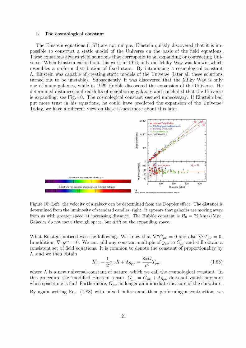
Figure 10: Left: the velocity of a galaxy can be determined from the Doppler effect. The distance isdetermined from the luminosity of standard candles; right: it appears that galaxies are moving awayfrom us with greater speed at increasing distance. The Hubble constant is H0 = 72 km/s/Mpc.Galaxies do not move through space, but drift on the expanding space.

What Einstein noticed was the following. We know that ∇µGµν = 0 and also ∇µTµν = 0.In addition, ∇µgµν = 0. We can add any constant multiple of gµν to Gµν and still obtain aconsistent set of field equations. It is common to denote the constant of proportionality byΛ, and we then obtain

Rµν −1

2gµνR + Λgµν =

8πG

c4Tµν , (1.88)

where Λ is a new universal constant of nature, which we call the cosmological constant. Inthis procedure the ‘modified Einstein tensor’ G′µν = Gµν + Λgµν does not vanish anymorewhen spacetime is flat! Furthermore, Gµν no longer an immediate measure of the curvature.

By again writing Eq. (1.88) with mixed indices and then performing a contraction, we

21

obtain R = 8πGc4T + 4Λ. Inserting this in Eq. (1.88) yields

Rµν =8πG

c4

(Tµν −

1

2Tgµν

)+ Λgµν . (1.89)

We now carry out the same procedure as in section I H and obtain the field equations in theweak-field limit for Newtonian gravitation

∇2Φ = 4πGρ− Λc2. (1.90)

For a spherical mass M we obtain for the gravitational field

~g = ∇Φ = −3GM

2r2~r + c2Λr~r, (1.91)

and we conclude that the cosmological term corresponds to a gravitational repulsion, whosestrength increases proportional to r.

Today we have a different view of the cosmological constant. Note that the energy-momentum tensor of a perfect fluid is given by

T µν =

(ρ+

P

c2

)UµUν + Pgµν . (1.92)

We imagine that a certain ‘substance’ exists with the curious equation of state P = ρc2. Wenever encountered such a substance, since it has a negative pressure! The energy-momentumtensor of this substance is given by

Tµν = −Pgµν = ρc2gµν . (1.93)

Here, we note the following. Firstly, the energy-momentum of this substance only dependson the metric tensor: it is a property of the vacuum itself and we denote by ρ the energydensity of the vacuum. Secondly, the expression for Tµν is identical to that for the constantcosmological term in Eq. (1.88). We can view the cosmological constant as a universalconstant that determines the energy density of the vacuum,

ρvacuumc2 =

Λc4

8πG. (1.94)

Denoting the energy-momentum density of the vacuum by T vacuumµν = ρvacuumc

2gµν , we canwrite the modified field equations as

Rµν −1

2Rgµν =

8πG

c4

(Tµν + T vacuum

µν

), (1.95)

with Tµν the energy-momentum tensor of matter and radiation.

If it is the case that Λ 6= 0, then at least it must small enough that ρvacuum has negligiblegravitational effects (|ρvacuum| < ρmatter) in situations where Newtonian gravitational theorygives a good description of the data. Systems with smallest densities where Newton’s lawscan be applied, are small clusters of galaxies. In this manner we can pose the following limit

|ρvacuumc2| =

∣∣∣∣ Λc4

8πG

∣∣∣∣ ≤ ρcluster ∼ 10−26 g/cm−3 (1.96)

22

Figure 11: History of the expansion of the Universe. In the past the effect of the mass densitywas more important that that of the cosmological constant and this delayed the expansion of theUniverse. However, when the volume of the Universe increases, then the density decreases. Theeffect of vacuum energy is constant. When the volume is sufficiently large then the Universe willexpand forever.

for the magnitude of the cosmological parameter. It is evident that if Λ is sufficiently small,it is completely unimportant on the scale of a star. However, as will become clear later on,it need not be negligible compared to the average matter density of the Universe as a whole(since it mostly consists of empty space!), and at very large scales it can have importanteffects on the evolution of the curvature of the Universe.

How can we calculate the energy density of the vacuum? The simplest calculations sum overall zero-point energies of all quantum fields known in Nature. The resulting answer exceedsthe upper limit on Λ that we just determined by about 120 orders of magnitude. This isnot understood and a physical principle must exist that makes the cosmological constantsmall. Recent data indicate that the cosmological constant does not vanish. The strongestindications come from measurements of distant Type Ia supernovae, which indicate that theexpansion of the Universe at this moment increases. This is outlined in Fig. 11. Without acosmological constant we expect that the attractive force between all matter in the Universeshould slow down the expansion and perhaps even lead to a contraction of the Universe.However, when the cosmological constant does not vanish, then the negative pressure of thevacuum can cause the expansion of the Universe to increase.

J. Alternative relativistic theories of gravity

The Einstein equations are not unique, as we have seen in the previous sections. It is alsopossible to construct radically new theories of gravity. We discuss a few of these in what

23

follows.

1. Scalar theories of gravity

In the Newtonian description of gravitation, the gravitational field is represented by thescalar Φ. This field obeys Poisson’s equation∇2Φ = 4πGρ. Because matter can be describedrelativistically by the energy-momentum tensor Tµν , the only scalar with the dimension ofmass density that we can construct is T µµ. Furthermore, position and time are components

of the 4-vector xµ and we can accommodate the time derivative via 2 ≡ ∇µ∇µ = −∂2ct+∇2.

A consistent scalar relativistic theory of gravity is given by the field equation

22Φ = −4πG

c2T µµ. (1.97)

This theory turned out to be incorrect (and for example predicted effects for the orbit ofMercury that were not observed). Furthermore, there is no coupling between gravitationand electromagnetism. Therefore, no gravitational redshift or bending of light by matter isincluded.

2. Brans - Dicke theory

A theory of gravitation based on a vector field can be excluded, since such a theory pre-dicts that massive particles will repel instead of attract. However, it is possible to formulatea relativistic theory that combines scalar, vector and tensor fields. The most importantexample of this type of theories is the one formulated by Robert Dicke and Carl Brans in1961. Brans and Dicke started in the construction of their theory from the equivalence prin-ciple and obtained a description of gravitation in terms of curvature of spacetime. However,instead of treating the gravitational constant G as a constant of Nature, they introduced ascalar field φ that determines the strength of G. This implies that the scalar field φ determ-ines the strength of the coupling of matter to gravitation. The coupled equations for thescalar field and the gravitational field can be written as

22φ = −4πλ(TM)µµ,

Rµν − 12gµνR = 8π

c4φ

(TMµν + T φµν

).

(1.98)

We observe that the effects of matter can be represented by the energy-momentum tensorTMµν and a coupling constant λ that determines the scalar field. The scalar field determinesthe magnitude of G and the field equations relate the curvature to the energy-momentumtensors of the scalar field (T φµν) and of matter (TMµν ). Historically, the coupling constant iswritten as λ = 2/(3 + 2ω). In the limit ω →∞ we obtain λ→ 0, and φ is not influenced bythe matter distribution. We then can set φ equal to φ = 1/G. In the limit ω → 0 we havethat T φµν → 0 and the Brans-Dicke theory reduces to that of Einstein.

The Brans-Dicke theory is important, since it shows that it is possible to develop altern-ative theories that are consistent with the equivalence principle. One of the predictions ofthe Brans-Dicke theory is that the effective gravitational constant G is a function of timeand is determined by the scalar field φ. A change in G could influence the orbits of planets

24

and a reasonable conservative conclusion from the data is that ω ≥ 500. This seems toindicate that Einstein’s theory is the correct theory of gravitation at least at relatively lowenergies.

3. Torsion theories

In our discussion of curved spacetime we assumed that the manifold has no torsion. Thisis not a necessary demand, and we can generalize the discussion of spacetime with a torsiontensor,

T µνσ = Γµνσ − Γµσν , (1.99)

that does not vanish. Typically, torsion is caused by the quantum mechanical spin ofparticles. Such theories are complicated mathematically. Gravitational theories with space-time torsion are often called Einstein-Cartan theories and have been investigated extensively.So far no evidence for torsion has been observed.

25

II. COSMOLOGY

A. The Universe at large scales

General relativity has had an important impact on our understanding of the Universe. In-deed, when looking at the Universe in its entirety, it is necessary to invoke general relativity.Roughly speaking, Newtonian gravity is adequate as long as the mass M of a system is smallcompared to its size R, or more precisely when the natural length scale GM/c2 associatedwith the mass is small compared to R: GM/c2R 1. General relativity becomes importantwhen this condition breaks down. This could happen for moderate values of GM/c2 if R issmall, which is the case with neutron stars and black holes, as we shall discuss later. Theother case is cosmology: if space is filled with matter of roughly the same density everywherethen the mass increases with R3, and GM/c2R must eventually get large.

Suppose we start increasing R from the center of the Sun. The Sun is not a relativisticobject in the above sense (check this!), and once R > R then M hardly increases untilthe next star is reached. Going on in this way, R will eventually encompass the Milky Waygalaxy, which contains some 1011 stars in a radius of roughly 15 kpc. Hence, for the galaxy,GM/c2R ∼ 10−6, so that the dynamics of the galaxy does not need a relativistic description.Galaxies themselves congregate in clusters, with a typical diameter of a Mpc. This is muchsmaller than the distances our telescopes are capable of seeing, which are in the order of105 Mpc. As it turns out, averaging over distances of 103 Mpc the Universe appears to bemore or less the same everywhere. The density of the Universe at this scale is not knownvery well, but has been estimated to be at least8 ρ = 10−28 kgm−3. With this density,GM/c2 = 4πGρR3/c2 starts becoming significantly larger than R for R ∼ 1027m ∼ 104

Mpc. This is comparable to the distances to which our telescopes can see, hence we needgeneral relativity.

The length scale at which the Universe starts appearing uniform, 103 Mpc, is much smallerthan the distance to which we can see, about 105 Mpc. Hence at the largest length scales,the universe appears homogeneous. Moreover, at such scales the Universe also appears tobe isotropic about every point: local observations will not reveal great differences betweendifferent directions in the sky. Finally, as shown by Edwin Hubble, the Universe is expanding.It could have been the case that at a given point, one would see a larger recessional velocityin one direction than in some other direction. This is not what we see at our location: allgalaxies appear to be receding from us with a velocity v related to their distance d by9

v = H0d, (2.1)

where H0 ' 70 kms−1Mpc−1. Now, assuming that we are at no special location in theUniverse, everything should be receding from everybody else, and isotropy continues tohold.

8 The reason for the uncertainty is that so far we have only been able to study the Universe in the electro-magnetic spectrum, so that a priori we can only “count” the mass that emits electromagnetic radiation.However, there is indirect evidence of copious amounts of dark matter and the number we give for thedensity is likely to be a severe underestimate.

9 This relationship, called Hubble’s law, is only valid for relatively small distances – hundreds of Mpc –after which it must be replaced by a different one which properly takes into account the curvature of theUniverse, about which more will be said later.

26

B. The topology of the Universe

Even if the Universe appears homogeneous and isotropic to observers in galaxies, it ispossible in principle to have an observer moving at relativistic velocities with respect to these.Such an observer would not see galaxies recede in all directions according to Eq. 2.1. Theassumption of homogeneity and isotropy must refer to a particular choice of time coordinatet such that hypersurfaces of constant t are homogeneous and isotropic. Thus, there is a“preferred” way of slicing the 4-dimensional spacetime of the Universe into 3-dimensionalslices, with galaxies as “markers”. In what follows, we will assume that

1. Spacetime can be sliced into hypersurfaces of constant time t which are perfectlyhomogeneous and isotropic; and

2. The mean rest frame of the galaxies agrees with the definition of simultaneity impliedby this particular time coordinate t.

One can then introduce spatial coordinates xi, i = 1, 2, 3 “anchored” to galaxies: eachgalaxy has fixed xi.10 These are called co-moving coordinates. Due to homogeneity, thespatial geometry of a constant t hypersurface can only depend on t, not on the spatialcoordinates, so that

dl2 = γij(t) dxidxj. (2.2)

Because of isotropy, all the components of γij(t) must increase at the same rate, withoutthere being a preferred direction, hence

dl2 = a2(t) γij dxidxj, (2.3)

where γij is independent of time. The line element for spacetime as a whole is11

ds2 = −dt2 + a2(t) γij dxidxj. (2.4)

Note that there can not be a cross term involving dt dxi because we would like the notion ofsimulaneity defined by t = const to agree with that of the local Lorentz frame of a galaxy.Since we also set g00 = −1, t is the proper time along a line dxi = const, i.e., it is the propertime of the galaxies.

Homogeneity and isotropy also imply that on the t = const slices we can choose an originwherever we please, and γij must be spherically symmetric about that origin. It is notdifficult to see that the most general spherically symmetric line element can be expressed as

γij dxidxj = e2f(r)dr2 + r2dΩ2, (2.5)

with dΩ2 = dθ2 + sin2(θ) dφ2. Again demanding homogeneity, we want the scalar curvature(3)R of γij to be a constant. A straightforward calculation shows that

(3)R = −2

[− 1

r2e2f (1− e−2f ) e−2f − 2re−2ff ′r−2

]=

2

r2

[1− e−2f (1− 2rf ′)

]=

2

r2

[r(1− e−2f )

]′, (2.6)

10 This is not in contradiction with the expansion of the Universe; it simply implies that the spatial coordinategrid expands in tandem with it.

11 For computational convenience, in this chapter we choose units such that c = G = 1.

27

where ′ = d/dr. Setting this equal to some constant K we get

K =2

r2

[r(1− e−2f )

]′(2.7)

which can be integrated to

γrr = e2f =

[1− 1

6Kr2 − A

r

](2.8)

where A is an integration constant. Demanding local flatness at r = 0, γrr(r = 0) = 0, weget A = 0. Writing k = K/6 we arrive at

γrr =1

1− kr2. (2.9)

Substituting this back into (2.4), we find the Friedman-Lemaıtre-Robertson-Walker (FLRW)line element

ds2 = −dt2 + a2(t)

[dr2

1− kr2+ r2dΩ2

]. (2.10)

Now note that whatever the value of k, we can always rescale it by a positive factor, withappropriate redefinition of both r and a(t). However, the sign of k can not be changed.Hence there are three different values of k we need to consider: k = +1, 0,−1. We nowdiscuss these possibilities in turn.

• k = 0. Then at any moment in time t0, the spatial line element is

dl2 = dr2 + r2dΩ2, (2.11)

where r = a(t0) r. This is the metric of a flat, 3-dimensional Euclidean space. Allt = const slices are spatially flat, and the geometry of the Universe is non-trivial onlythrough the time evolution of the 4-metric as a whole. This is the spatially flat FLRWmodel.

• k = +1. Define a coordinate χ(r) such that

dχ2 =dr2

1− r2. (2.12)

Solving for r one finds r = sin(χ) so that the spatial line element at a time t0 is

dl2 = a2(t0)[dχ2 + sin2(χ)

(dθ2 + sin2(θ) dφ2

)]. (2.13)

This is the metric of a three-sphere of radius a(t0), i.e., of a 3-dimensional hypersurfacein 4-dimensional Euclidean space whose Cartesian coordinates satisfy

x2 + y2 + z2 + w2 = a2(t0). (2.14)

The corresponding 4-metric is the closed FLRW model.

28

• k = −1. A similar coordinate transformation as above now gives

dl2 = a2(t0)[dχ2 + sinh2 χdΩ2

]. (2.15)

The corresponding 4-metric is the open FLRW model.

This model has an interesting property. χ is a radial coordinate, and when we increaseit, the circumferences of the two-dimensional spheres coordinatized by (θ, φ) increase assinh(χ). But sinh(χ) > χ for all χ > 0, hence the circumferences increase more rapidlywith radius than in flat space. The spatial metric dl2 describes a space which cannot berepresented as a 3-dimensional hypersurface of a flat, 4-dimensional Euclidean space.

The hyperbolic, flat, and spherical geometries are illustrated in Fig. 12.

Figure 12: An illustration of the hyperspherical, flat, and hyperbolic geometries, with one dimensionsuppressed (in reality they are of course 3D spaces).

C. The dynamics of the Universe

We now turn to the dynamics of the FLRW models as given by the Einstein equations.For this we need to specify an energy-momentum tensor Tµν . On cosmic scales, galaxiesbehave as a “gas” of particles to which we can assign a (average) density ρ. Neglectinginteractions between galaxies, the pressure P can be set to zero. This leads to

Tµν = ρ uµuν , (2.16)

where uµ is the 4-velocity of any given galaxy; in co-moving coordinates, uµ = (1, 0, 0, 0).This is the energy-momentum tensor of a perfect fluid with zero pressure. However, otherforms of mass-energy are also present in the Universe. For example, the Cosmic MicrowaveBackground represents a thermal distribution of radiation with a temperature of about 3K. This radiation can also be represented as a perfect fluid, but with non-zero pressure: formassless thermal radiation one has P = ρ/3. There may be other contributions to the totalenergy-momentum tensor, all of which we shall assume to be in the form of a perfect fluid.This leads us to write

Tµν = ρ uµuν + P (gµν + uµuν). (2.17)

This we substitute into the Einstein equations,

Gµν = Rµν −1

2gµνR = 8πTµν , (2.18)

29

which leads to

Gtt = 8πTtt = 8πρ,

Gxx = 8πTxx = 8πa2P. (2.19)

As a result of the high degree of symmetry, these are in fact the only two independentcomponents of the Einstein equations; all the others are either trivially satisfied or equivalentto one of the above. We now need to compute Gtt and Gxx in terms of a(t). Let us do thisexplicitly for the case of a flat spatial geometry, where the 4-metric can be written in theform

ds2 = −dt2 + a2(t)[dx2 + dy2 + dz2

]. (2.20)

The non-vanishing components of the Christoffel symbols are

Γtxx = Γtyy = Γtzz = aa,

Γxxt = Γxtx = Γyyt = Γyty = Γzzt = Γztz =a

a, (2.21)

with a = da/dt. The independent Ricci tensor components are then

Rtt = −3a

a,

Rxx = aa+ 2a2. (2.22)

The Ricci scalar is

R = −Rtt + 3a−2Rxx = 6

[a

a+a2

a2

], (2.23)

so that

Gtt = Rtt +1

2R = 3

a2

a2= 8πρ,

Gxx = Rxx −1

2a2R = −2aa− a2 = 8πa2P. (2.24)

Combining these equations we may write

3a

a= −4π(ρ+ 3P ). (2.25)

Repeating the calculation for the closed and open FLRW Universes, we find that in generalthey are governed by the following two equations:

a2

a2=

8π

3ρ− k

a2, (2.26)

a

a= −4π

3(ρ+ 3P ). (2.27)

The equations (2.27) immediately lead to a striking prediction. Provided that ρ > 0 andP ≥ 0, the Universe can not be static. Indeed, one will have a < 0, so that the Universe mustalways be either expanding (a > 0) or contracting (a < 0), except perhaps at an instantin time when expansion changes over to contraction. Note the nature of this expansion or

30

contraction: The distances between all co-moving observers (galaxies) change with time;there is no “center” or preferred point. If at time t the distance between two such observersis D, then

v ≡ dD

dt=D

a

da

dt= HD, (2.28)

where H(t) = a(t)/a(t) is the Hubble parameter. If the observers are sufficiently close (e.g.,at a distance of a few hundred Mpc) then we can approximate H by H0, its value at thecurrent epoch, and we retrieve Hubble’s law (2.1). As found by Hubble, the Universe iscurrently expanding, a > 0. According to Eq. (2.27), a < 0, so moving back in time theUniverse must have been expanding faster and faster. If the Universe had always expandedat the current rate, then at the time T = a/a = H−1

0 we would have had a = 0. Since theexpansion was actually faster, the time at which a = 0 was even closer to the present. Thus,under the assumption of homogeneity and isotropy, general relativity makes the predictionthat at a time less than H−1

0 ago, the Universe was in a singular state: The distance betweenall points in space was zero, and the density of matter as well as the curvature of spacetimewas infinite. This state is referred to as the Big Bang. For a while it was thought that ifthe assumptions of homogeneity and isotropy were relaxed, the Big Bang could be avoided,but it is now known that singularities are in fact generic features of cosmological solutions.

Eqns. (2.26) and (2.27) allow us to obtain an equation for the time evolution of the massdensity. Indeed, multiplying (2.26) by a2, differentiating with respect to t, and eliminatinga using (2.27), we find

ρ = −3(ρ+ P )a

a. (2.29)

Thus, for matter (P = 0), we getρ a3 = const, (2.30)

which expresses conservation of rest mass. For radiation (P = ρ/3), one has

ρa4 = const. (2.31)

Here the energy density decreases more rapidly than a3 as a grows, because the radiation ineach volume element does work on its surroundings as the Universe expands. Alternatively,in terms of photons, the photon number density decreases as a−3, but each photon losesenergy as a−1 due to cosmological redshift caused by the expansion; see below.

Let us discuss the qualitative features of the FLRW Universes depending on the value ofk. If k = 0 or −1, Eq. (2.26) tells us that a can never become zero. Indeed, for any matterwith P ≥ 0, ρ must decrease at least as rapidly as a−3, so that ρ a2 → 0 as a → ∞. Weconclude that if k = 0 (a flat Universe), the expansion rate a asymptotically approaches zeroas t → ∞, while if k = −1 we find a → 1 as t → ∞. In both cases the Universe expandsforever.

The situation is different for k = +1. The first term in the right hand side of Eq. (2.26)decreases more rapidly with a than the second term, and since the left hand side must bepositive, there is a critical value ac such that a ≤ ac. Furthermore, a cannot asymptoticallyapproach ac as t→∞ because the magnitude of a is bounded from below due to Eq. (2.27).Thus, if k = +1, then at a finite time after the Big Bang, the Universe will reach a maximumsize ac after which it will contract again. The same argument as above for the occurenceof a Big Bang now shows that a finite time after the recontraction begins, there must be aBig Crunch where once again a = 0. Thus, the spatially closed Universe can only exist fora finite (albeit possibly very long) time.

31

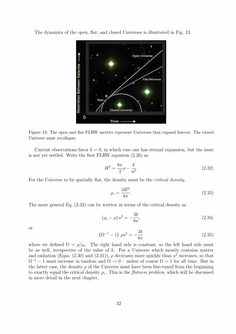
The dynamics of the open, flat, and closed Universes is illustrated in Fig. 13.

Figure 13: The open and flat FLRW metrics represent Universes that expand forever. The closedUniverse must recollapse.

Current observations favor k = 0, in which case one has eternal expansion, but the issueis not yet settled. Write the first FLRW equation (2.26) as

H2 =8π

3ρ− k

a2. (2.32)

For the Universe to be spatially flat, the density must be the critical density,

ρc =3H2

8π. (2.33)

The more general Eq. (2.32) can be written in terms of the critical density as

(ρc − ρ) a2 = −3k

8π, (2.34)

or (Ω−1 − 1

)ρa2 = −3k

8π(2.35)

where we defined Ω = ρ/ρc. The right hand side is constant, so the left hand side mustbe as well, irrespective of the value of k. For a Universe which mostly contains matterand radiation (Eqns. (2.30) and (2.31)), ρ decreases more quickly than a2 increases, so thatΩ−1 − 1 must increase in tandem and Ω → 0 – unless of course Ω = 1 for all time. But inthe latter case, the density ρ of the Universe must have been fine-tuned from the beginningto exactly equal the critical density ρc. This is the flatness problem, which will be discussedin more detail in the next chapter.

32

D. Dark energy

We have seen that if ρ > 0 and P ≤ 0, one has a < 0 on account of Eq. (2.27), so that theexpansion of the Universe should be slowing down. Since about a decade, evidence has beenaccumulating that the expansion of the universe is actually speeding up. One explanationcould be that there is a cosmological constant Λ in the Einstein equations:

Rµν −1

2gµνR + Λgµν =

8πG

c4Tµν . (2.36)

Einstein originally introduced the cosmological constant because of the then prevalent philo-sophical bias that the Universe should be forever stationary, whereas in standard generalrelativity, it needs to either expand or contract. With Λ < 0, a stationary Universe ispossible, although we now know that it would not be stable against small perturbations,again leading to either expansion or contraction. A non-stationary Universe is a predictionof general relativity, with or without a Λ term. After Hubble’s observations, Einstein calledthe introduction of the cosmological constant “the biggest blunder of his life”. However,recently the idea has been resurrected. Observations of distant supernovae revealed that,given their redshift, they are dimmer and hence more distant than they should be, suggest-ing an accelerated expansion of the Universe. Observations currently favor a small, positivecosmological constant, which would make gravity slightly repulsive on large scales and givespacetime a natural tendency to expand.

In the present of a cosmological constant, Eqns. (2.26) and (2.27) become(a

a

)2

=8π

3ρ− k

a2+

Λ

3, (2.37)

a

a= −4π

3(ρ+ 3P ) +

Λ

3, (2.38)

but Eq. (2.29) continues to hold as stated. Let us assume Λ > 0 and repeat the reasoningabove for the flat, open, and closed Universes. For k = +1, it is now possible that the secondterm in Eq. (2.37) will never come to dominate over the first and third, in which case theturnover point a = 0 is never reached and the Universe will expand forever. If a turnover isreached, it will be delayed compared to the case with Λ = 0. For k = 0 and k = −1, theUniverse will certainly keep expanding forever, just as in the Λ = 0 case. However, since ρand P go to zero as a→∞, there must come a time when the Λ term comes to dominate.After that one has a > 0: the expansion of the Universe will be accelerating.

Another possibility is dark energy, a putative new form of matter or energy with positivedensity but negative pressure. If you were to try to inflate a tyre by pumping dark energyinto it, the tyre would get heavier, but it would actually deflate; heuristically one can thinkof space being expelled from the tyre. At this point nothing is known about the nature ofdark energy12. As a first attempt to model it, one can think of it as being a perfect fluidwith equation of state

PDE = wρDE, (2.39)

with PDE the pressure, ρDE the density, and w < 0 the equation-of-state parameter. If w isconstant and equal to −1, then that is equivalent to having a cosmological constant Λ and

12 Not to be confused with dark matter, the origin of which is equally unclear.

33

there is no need to posit dark energy. However, w could be time-dependent, but even thatis something we have no knowledge of at present. From Eq. (2.29) we get

ρDE = −3a

a(1 + w)ρDE, (2.40)

and if w is constant (or slowly varying) this integrates to

ρDE = ρDE,0 a−3(1+w), (2.41)

with ρDE,0 the present-day density of dark energy. If w is non-constant then this can begeneralized with the replacement

a−3(1+w) → exp

(3

∫ 1

a

da′

a′[1 + w(a′)]

), (2.42)

where we set the present-day value of the scale factor a to 1.The Hubble parameter H = a

aneatly encapsulates the past history and dynamics of the

Universe. By means of Eq. (2.37) we can write

H2(a) = H20

[ΩMa

−3 + ΩRa−4 + Ωka

−2 + ΩDE exp

(3

∫ 1

a

da′

a′[1 + w(a′)]

)]. (2.43)

The dimensionless constants ΩM, ΩR, Ωk, and ΩDE are defined as

ΩM =8πGρM,0

3H20

, (2.44)

ΩR =8πGρR,0

3H20

, (2.45)

ΩDE =8πGρDE,0

3H20

, (2.46)

Ωk = − k

H20

. (2.47)

Here ρM,0 is the present-day value of the matter density, ρR,0 the same for radiation, andρDE,0 for the dark energy density. Later on we will talk about methods with which the aboveconstants can be determined. For now we mention that existing data points towards Ωk ' 0,ΩR ' 0, ΩM ' 0.27, and ΩDE ' 0.73. In other words, dark energy completely dominatesover matter! As discussed in the previous section, the density of dark energy (or, if w = −1,the density associated with the cosmological constant) must be extremely small, but theUniverse is mostly devoid of matter, and the average matter density turns out to be smallerthan that of dark energy. Note that as t→∞, having w = −1 would imply

limt→∞

H2(t) = lima→∞

H2(a) = H20 ΩDE, (2.48)

and since H(a) = a/a, this means

a = H0

√ΩDE a. (2.49)

Hence, at late times (much beyond the present epoch) the Universe will then end up under-going eternal exponential expansion:

a(t) = a0 exp[H0

√ΩDE t

]. (2.50)

34

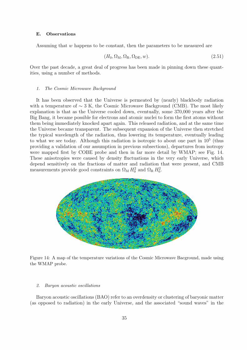
E. Observations

Assuming that w happens to be constant, then the parameters to be measured are

(H0,ΩM,ΩR,ΩDE, w). (2.51)

Over the past decade, a great deal of progress has been made in pinning down these quant-ities, using a number of methods.

1. The Cosmic Microwave Background

It has been observed that the Universe is permeated by (nearly) blackbody radiationwith a temperature of ∼ 3 K, the Cosmic Microwave Background (CMB). The most likelyexplanation is that as the Universe cooled down, eventually, some 370,000 years after theBig Bang, it became possible for electrons and atomic nuclei to form the first atoms withoutthem being immediately knocked apart again. This released radiation, and at the same timethe Universe became transparent. The subsequent expansion of the Universe then stretchedthe typical wavelength of the radiation, thus lowering its temperature, eventually leadingto what we see today. Although this radiation is isotropic to about one part in 105 (thusproviding a validation of our assumption in previous subsections), departures from isotropywere mapped first by COBE probe and then in far more detail by WMAP; see Fig. 14.These anisotropies were caused by density fluctuations in the very early Universe, whichdepend sensitively on the fractions of matter and radiation that were present, and CMBmeasurements provide good constraints on ΩM H2

0 and ΩRH20 .

Figure 14: A map of the temperature variations of the Cosmic Microwave Bacground, made usingthe WMAP probe.

2. Baryon acoustic oscillations

Baryon acoustic oscillations (BAO) refer to an overdensity or clustering of baryonic matter(as opposed to radiation) in the early Universe, and the associated “sound waves” in the

35

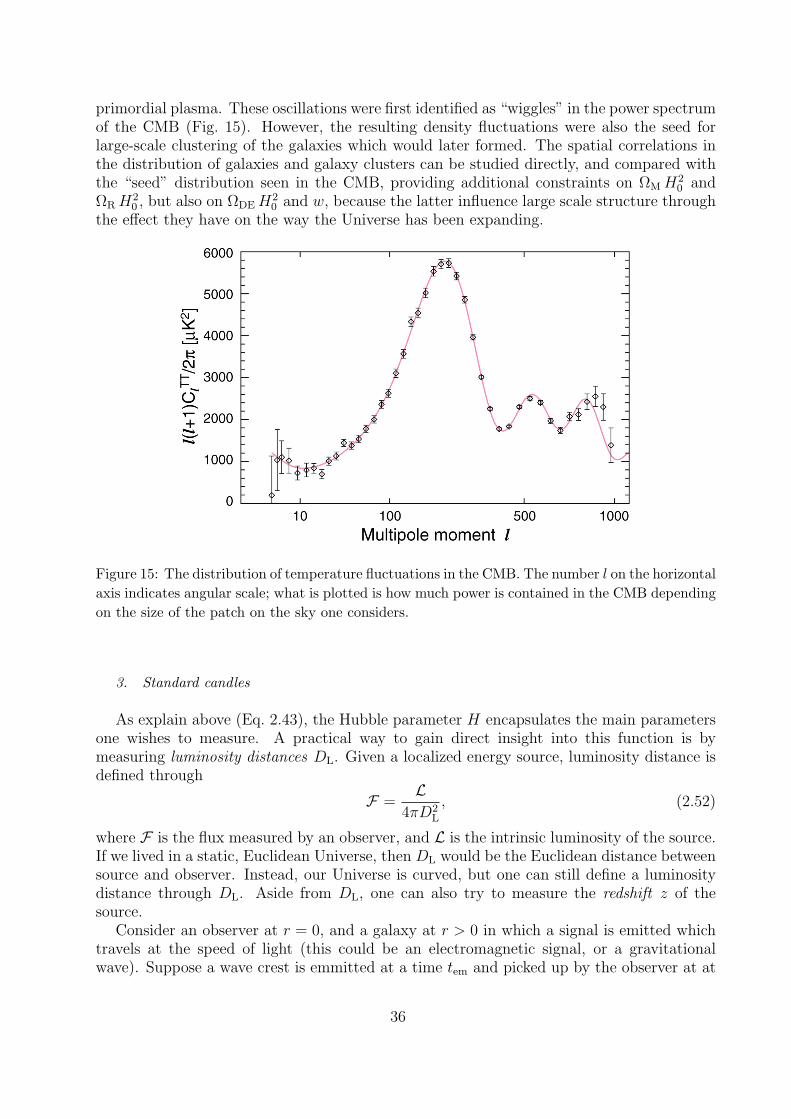
primordial plasma. These oscillations were first identified as “wiggles” in the power spectrumof the CMB (Fig. 15). However, the resulting density fluctuations were also the seed forlarge-scale clustering of the galaxies which would later formed. The spatial correlations inthe distribution of galaxies and galaxy clusters can be studied directly, and compared withthe “seed” distribution seen in the CMB, providing additional constraints on ΩM H2

0 andΩRH

20 , but also on ΩDEH

20 and w, because the latter influence large scale structure through

the effect they have on the way the Universe has been expanding.

Figure 15: The distribution of temperature fluctuations in the CMB. The number l on the horizontalaxis indicates angular scale; what is plotted is how much power is contained in the CMB dependingon the size of the patch on the sky one considers.

3. Standard candles

As explain above (Eq. 2.43), the Hubble parameter H encapsulates the main parametersone wishes to measure. A practical way to gain direct insight into this function is bymeasuring luminosity distances DL. Given a localized energy source, luminosity distance isdefined through

F =L

4πD2L

, (2.52)

where F is the flux measured by an observer, and L is the intrinsic luminosity of the source.If we lived in a static, Euclidean Universe, then DL would be the Euclidean distance betweensource and observer. Instead, our Universe is curved, but one can still define a luminositydistance through DL. Aside from DL, one can also try to measure the redshift z of thesource.

Consider an observer at r = 0, and a galaxy at r > 0 in which a signal is emitted whichtravels at the speed of light (this could be an electromagnetic signal, or a gravitationalwave). Suppose a wave crest is emmitted at a time tem and picked up by the observer at at

36

time tobs. Setting ds2 = 0, we have∫ tobs

tem

cdt

a(t)=

∫ r

0

dr

(1− kr2)1/2. (2.53)

If a second wave crest is emitted at a time tem + ∆tem and absorbed at a time tobs + ∆tobs,∫ tobs+∆tobs

tem+∆tem

cdt

a(t)=

∫ r

0

dr

(1− kr2)1/2. (2.54)

The right hand sides of (2.53) and (2.54) are the same, since observer and source are at fixedco-moving positions. Taking the difference between the two equations, to leading order in∆tem and ∆tobs one has

∆tobs =a(tobs)

a(tem)∆tem. (2.55)

In an expanding Universe a(tobs) > a(tem), so that there is a time dilation effect: the timebetween wave crests will be larger at the observer. The redshift z is defined by

1 + z =a(tobs)

a(tem). (2.56)

The time dilation implies that according to the observer’s clock, a clock at the source willbe slower by a factor 1 + z:

dtobs = (1 + z) dts. (2.57)

The frequency seen by the observer will then also be lower than at the source,

fobs =fs

1 + z. (2.58)

Energies are similarly affected13:

Eobs =Eem

1 + z. (2.59)

Together with (2.57), this allows us to relate the emitted power to the observed one:

dEobs

dt=

1

(1 + z)2

dEem

dtem

(2.60)

The flux at the observer is given by

F =1

A

dEobs

dtobs

, (2.61)

where A = 4πa2(tobs)r2 is the area over which a wavefront will have spread when the signal

reaches the observer. Hence

F =L

4πa2(tobs)r2(1 + z)2, (2.62)

13 The easiest way to see this is to use the quantum relation E = hf , but it can also be derived classically

37

with L = dEem/dtem the intrinsic luminosity of the source. From the definition of luminositydistance, Eq. (2.52), we find

DL = (1 + z)a(tobs) r. (2.63)

In the rest of this chapter we specialize to the case of a flat universe, k = 0. Then∫ tobs

tem

cdt

a(t)= r. (2.64)

Time and redshift are related as

1 + z(t) =a(tobs)

a(t), (2.65)

and differentiating we getdt

a(t)= − 1

a(tobs)

dz

H(z), (2.66)

where the Hubble parameter is defined as

H(z) =a(z)

a(z), (2.67)

and a dot denotes derivation with respect to t. Eq. (2.64) can then be written as

a(tobs) r = c

∫ z

0

dz′

H(z′), (2.68)

so that

DL = c(1 + z)

∫ z

0

dz′

H(z′). (2.69)

For small z, Eq. (2.69) yieldsH0DL ' cz, (2.70)

which with vrec = cz again gives Hubble’s law. However, the more general expression (2.69)contains far more information; in fact, it encapsulates the entire past dynamics and geometryof the Universe through its dependence on H(z):

DL = DL(z;H0,ΩM,ΩR,Ωk, ρDE, w). (2.71)

If one has a sufficient number of sources for which DL and z can be measured by independentmeans, then one can fitDL as a function of z withH0, ΩM, ΩR, Ωk, ΩDE, w as free parameters.This way the values of the latter can be measured, as the numbers that lead to the best fitfor DL(z).14

One way to make such measurements is to consider Type Ia supernovae. These arebelieved to always have the same intrinsic luminosity, to within 10% or so. From theirspectrum (or that of the host galaxy) one can also infer their redshift with essentially zerouncertainty. Thus, they are standard candles : DL and z can be measured separately. A

14 Although in the derivation of Eq. (2.69) we assumed a flat Universe, the expression is more generallyvalid.

38

problem is that Type Ia supernovae will have been slightly different in the past, when starshad not yet produced as many heavy elements as there are today. The luminosity of Type Iasupernovae needs to be calibrated, which necessitates measuring... their distance. This canbe done by looking at the galaxies they live in. For spiral galaxies, there exists a relationshipbetween their size and the velocities with which their stars move – the Tully-Fisher relation.The latter can be established by Doppler shift measurements, which then provides a wayto measure lumonosity distance. However, this relationship is itself in need of calibration,once again requiring distance measurements by alternative means. The distances to close-bygalaxies are measured by observing variable stars called Cepheids. The average brightnessof a Cepheid is closely related to the period with which it brightens an dims, from whichluminosity distance can be inferred. But this relationship also needs to be calibrated, whichis done by parallax measurements on Cepheids in our own galaxy. As the Earth movesaround the Sun, the apparent position of a star in the sky traces out an ellipse, and theangular size of this ellipse is a measure of distance. Parallax measurements are accurate outto a few kpc, allowing for the calibration of nearby Cepheids. Beyond that one relies on thisCepheid calibration for distance measurements up to about 10 Mpc. The number of spiralgalaxies within that distance is sufficient to calibrate the Tully-Fisher relation, which is thenused on its own to measure distances up to tens of Mpc. Finally, Type Ia supernovae arecalibrated. Thus, measurements of DL rely on an entire cosmic distance ladder ; see Fig. 16.Each step of the ladder comes with statistical as well as systematic uncertainties, related to,e.g., the absorption of light as it travels to us. Nevertheless, supernovae have proven to beuseful in further constraining cosmological parameters.

Figure 16: The so-called cosmic distance ladder, which is used to calibrate faraway standard candlessuch as Type Ia supernovae.

Combining the results from WMAP, BAO, and supernovae, the following informationwas obtained:

• The age of the Universe is 13.72± 0.12 billion years;

• The total matter content of the Universe is ΩM = 0.27± 0.02. Of this, less than 20%is ordinary, baryonic matter. The rest is dark matter (not to be confused with dark

39

energy!) which doesn’t seem to emit light but makes its presence known through itsgravitational pull. The nature of dark matter is as yet unclear;

• The radiation content is tiny, ΩR ∼ 5×10−5; although radiation would have dominatedin the very early Universe (due to the a−4 dependence of the density on the scalefactor), at the current epoch its effects are negligible;

• The dark energy contribution is ΩDE = 0.73±0.02. Note that ΩM +ΩDE = 1 to withinthe stated accuracies. Since necessarily the sum of all the Ω’s must be 1, this suggestsΩk = 0, i.e., a flat Universe;

• One has −1.11 < w < −0.86. Hence the dark energy could be a cosmological constant– corresponding to w = −1 – but other values of w (and indeed a time-dependent w)are clearly still allowed.

The assumption that at large length scales, the past history and dynamics of the Universeis well described by one of the FLRW spacetimes, together with the above constraints, isreferred to as the Standard Model of Cosmology.

4. Future measurements

Later on we will talk about gravitational waves (GW), “ripples” in the curvature ofspacetime which propagate at the speed of light. In the future these could revolutionize ourunderstanding of the Universe, in various ways.

• Primordial gravitational waves should have been created within a Planck time (∼5 × 10−44 s) of the Big Bang, to be compared with the CMB which originated some370,000 years later. Thus, a cosmological GW background could provide informationabout what happened at the very instant of the Big Bang, when quantum gravityeffects were still strong. This might help us in understanding how quantum mechanicsand GR are to be reconciled and combined into one theory. Also, phase transitionsin the early Universe associated with the decoupling of the electroweak force15, whichhappened some 10−10 s after the Big Bang, could have created a GW background. Suchprimordial GW may have left an imprint on the electromagnetic Cosmic MicrowaveBackground through its polarization. An important goal of the Planck probe, whichwas launched in 2009, is to study the polarization of the CMB. Alternatively (or inaddition), primordial GW may be found by dedicated gravitational wave detectorsthat are currently operational and under construction.

• The direct detection of GW may also give us a new kind of standard candle. Binarysystems consisting of two neutron stars, a neutron star and a black hole, or twoblack holes tend to spiral towards each other as they lose orbital energy through GWemission, and eventually they merge to form a single black hole, leading to even moregravitational radiation. Such systems are self-calibrating, in the sense that the distancecan be deduced from the gravitational waveform itself, with no reference to any kind

15 Quantum field theory tells us that electromagnetism and the weak nuclear force were once just one singleinteraction.

40

of cosmic distance ladder. If the host galaxy in which the coalescence event took placecan be separately identified and its redshift z measured, then the relationship (2.71)can be used to constrain cosmological parameters directly. In a later chapter we willstudy in detail how this is to be done.

41

III. COSMOLOGICAL INFLATION

The Standard Model of Cosmology yields a global picture of the evolution of the Universe.However, it suffers from several subtle, but serious shortcomings. We will investigate thisand discover how cosmological inflation presents a solution. Details of inflation are modeldependent. Next, we describe an elementary model for the inflation process. We derivethe duration of the inflation epoch and study the connection, through reheating, to the BigBang model discussed previously.

A. Shortcomings of the Standard Model of Cosmology

When considered by itself, there are a number of problems with the Standard Model ofCosmology:

• Horizon problem: the horizon of an observer is the largest distance over which aninfluence, any influence, can have travelled in order to reach this observer. It presentsan upper limit to the volume of space that can be in causal contact with the observer.We have already seen that no influence can travel faster than light, and thus it followsthat the horizon of an observer represents the size of the visible Universe of thisobserver.

Thermal equilibrium between different parts of the Universe can only be establishedthrough the exchange of photons of the cosmic microwave background radiation. How-ever, these photons decoupled from matter around 105 years after the Big Bang: afterthis event it was not possible anymore to bring different parts of the Universe inthermal equilibrium. During this decoupling, the horizon of an observer was manytimes smaller than it is today. Thus, we expect that regions with photons of sim-ilar temperatures are much smaller that the present visible Universe. The oppositeappears to be true: data show that the entire visible Universe has nearly the sametemperature (we have used this fact before to justify the cosmological principle). Theresulting paradox is called the horizon problem.

• Flatness problem: data show that the present Universe has a metric that is extremelyflat: the flat Robertson-Walker metric. We have already calculated that the expansionof the Universe predicts that the curvature becomes increasingly smaller: Ω→ 0 whent becomes larger. This implies that, in order to explain the present flatness, themetric of the early Universe resembled even more that of the perfect flat Robertson-Walker metric. This is known as the flatness problem: which mechanism brought theearliest magnitude of flatness so close to that of the perfect Robertson-Walker value?This question can be evaded by assuming that the Universe was always perfectly flat.However, this then leads to the question why did the Universe start off with exactly thecritical density? The Standard Model of Cosmology does not answer these questions.

• Missing particles: many of the modern particle physics theories predict the existence ofexotic particles that have not been discovered so far. Examples include supersymmetricparticles and magnetic monopoles. Typically, these particles are extremely massiveand are therefore difficult (or impossible at this moment) to create with accelerators.However, in the early Universe temperatures may have been high enough to allow

42

natural creation of such particles. So far, none of these particles have been observed16.This raises the question: if such particles were indeed produced in the early Universe,why do we not find them today?

All these problems can be solved at once when we expand the Standard Model of Cosmo-logy with a new concept: cosmological inflation. This is the assumption that the Universe,immediately after the Big Bang, has had a period of extreme rapid expansion. Mathemat-ically, we can define this as follows: during inflation17

a(t) > 0, a(t) > 0. (3.1)

By introducing inflation, we can solve the three shortcomings of the Standard Model. Thehorizon problem is solved by the fact that during inflation the scale factor a(t) becomesextremely large. This implies that parts of the Universe that already had established thermalequilibrium before the start of inflation, inflated to much larger proportions than the horizonof an observer in this part of the Universe. The consequence is then that after inflation ends,the visible Universe for this observer is fully in equilibrium, exactly as the data show today!

The flatness problem is solved by the fact that every manifold, when expanded to suffi-ciently large proportions, appears flat to a local observer. This is in complete analogy withthe surface of the Earth, which is sufficiently large compared to local observers, and appearsflat to us.

Finally, the problem of missing particles is solved in a trivial manner through the in-troduction of an inflationary period. When the Universe is expanded by vast amounts, allexotic particles that were created before the start of inflation will be distributed over a largevolume. This makes the probability to encounter such a particle in an Earth-bound detectorvery small. Clearly, inflation only explains why the initial exotic particles are not found,and it makes no statement about particles that may have been created after inflation ended.Note that we do not expect such particles to have been created at these later times. Typ-ically, exotic particles have such high masses that their creation is prevented in a Universewhere the energy density has significantly decreased because of expansion.

B. The dynamics of cosmological inflation

We will now discuss how cosmological inflation can be realized: how can we apply theFriedmann equations to obtain inflation? We have already seen during our discussion of thecosmological constant that energy with an equation of state P = −ρ yields an exponentiallyexpanding Universe. However, this is not the only way to satisfy Eq. (3.1). When we considerthe second Friedmann equation (2.27), we see that inflation occurs when the right-hand sideof this equation is positive. In terms of the equation of state this means that inflation occursfor all matter and energy that has the property P = nρ with n < −1

3.

16 Discovery of magnetic monopoles has been claimed by some experimental physicists, however their resultcould never be reproduced.

17 Note that a Universe with a cosmological constant obeys this definition, and we could denote our presentexpansion as inflation. However, we will reserve the term inflation for accelerated expansion of the early

Universe.

43

Such energy is not encountered in classical physics. However, in quantum physics it ispossible to realize such types of energy, through a description in terms of fields instead ofparticles. We will now define a field that is constructed in such a manner that it has anenergy density and pressure that obey an equation of state in which n < −1

3. It is then up

to experimental physics to show whether such a field exists in Nature.The model that is employed the most consists of a scalar field Φ(t) which only depends

on time and not on space. The cosmological principle suggests that all energy and mattershould be distributed homogeneously and isotropically. The choice for a vector or tensor fieldwould not be in agreement with the demand for isotropy because of the rotation dependenceof such fields. Spatial dependence would be in conflict with the demand for homogeneity. Ascalar field has a Lagrangian density given by18

L = −1

2gµν(∂µΦ(t)

)(∂νΦ(t)

)− V

(Φ(t)

), (3.2)

where in the present case none of the spatial derivatives contribute. Every Lagrangiandensity has a corresponding action S, given by

S =

∫d3xdt

√−g L (3.3)

where g is the determinant of the metric. In the present case we employ the flat Robertson-Walker metric, and the determinant is given by

g = −a6(t). (3.4)

With the Euler-Lagrange equations we can now derive the equations of motion for the scalarfield Φ(t). This is a long calculation, although relatively simple since the field only dependson time. The scalar field Φ(t) evolves in time according to the equation of motion

Φ(t) + 3a(t)

a(t)Φ(t) + c2∂ΦV

(Φ(t)

)= 0. (3.5)

Note that the details of the evolution of the scalar field depend on the potential energydensity V

(Φ(t)

). The various types of models for cosmological inflation are characterized

by the choice of this quantity. Here we will not enter into details and in the following we willnot make explicit assumptions for the shape of V

(Φ(t)

). Consequently, all our conclusions

are generic.Each Lagrangian density leads to an energy-momentum tensor

Tµν =(∂µΦ

)(∂νΦ

)+ gµνL. (3.6)

This expression can be used to calculate the pressure and density due to the scalar field.We insert our current Langrangian density and metric, and compare the resulting energy-momentum tensor with that of the Friedmann fluid. The expression for the pressure anddensity can then be directly read off. We find

ρ(t) =1

2

1

c2Φ2(t) + V

(Φ(t)

),

P (t) =1

2

1

c2Φ2(t)− V

(Φ(t)

). (3.7)

18 Note that for a scalar field one has ∇µΦ = ∂µΦ.

44

Note that the first term can be seen as the kinetic energy density of the scalar field, and thesecond as the potential energy density. The expression for the density ρ of the total energyis in excellent agreement with our expectation19.

We consider a Universe that, in its earliest epoch, is filled with the usual types of energy:cold matter, radiation, a cosmological constant, and now add an inflaton field. All theseinfluences determine, through the Friedmann equations, the evolution of the scale factorwith time. When the influence of the inflaton field is dominant, then the Universe will entera period of exponential expansion. The results is that the other influences can immediatelybe neglected. Surely, the energy density and pressure of the usual forms of energy andmatter are proportional to the inverse of the scale factor to a certain power and thereforewill asymptotically (and rapidly for typical inflation models) vanish. Therefore, all termsin the Friedmann equations that are proportional to pressure and density can be neglectedin the description of the Universe in an inflationary period. Consequently, we concludethat the Universe in an inflationary period can be described by the Friedmann equationssubstituting only the influence of the inflaton field, and, obviously, the equations of motionfor that inflaton field, see Eq. (3.5). The resulting set of equations of motion are called theinflation equations

Φ(t) + 3H(t)Φ(t) + c2∂ΦV(Φ(t)

)= 0,

H2(t) =8πG

3c2

(1

2

1

c2Φ2(t) + V

(Φ(t)

)). (3.8)

We can summarize inflation cosmology as follows: argue for a particular expression forthe potential energy density V

(Φ(t)

), substitute this into the inflation equations, solve the

resulting set of equations of motion in order to obtain the explicit expression for the scalefactor a(t) and the inflaton field Φ(t).

Note that it is not guaranteed that a solution a(t), Φ(t) indeed describes inflation (a(t) >0, a(t) > 0) for each arbitrary shape of the potential energy density V (Φ(t)). In the nextsection we will therefore derive criteria that, when obeyed, guarantee inflation.

C. Simplified inflation equations

Next, we consider the question in which manner a scalar field can be used to realizeinflation. This is not a trivial question: we have already seen that inflation occurs whendensity and pressure lead to an equation of state with n < −1

3, but both quantities depend in

a non-trivial manner on the magnitude of the scalar field Φ(t), which itself is dictated by theequations of motion. It is for this reason that at present one often makes the assumption ofslow evolution20: it is assumed that the scalar field slowly evolves in time, in such a mannerthat we may assume that the Φ terms in Eq. (3.7) for density and pressure can be neglected(this implies that the kinetic energy of the field is much smaller that its potential energy),

1

2

1

c2Φ2(t) V

(Φ(t)

). (3.9)

19 The expressions for the density and pressure can also be obtained by assuming that ρ obeys this expression,and then, as we have demonstrated before, use the Friedmann equations to find the corresponding pressure.

20 The so-called Slow Roll Condition.

45

One then has

ρ(t) ≈ +V(Φ(t)

),

P (t) ≈ −V(Φ(t)

). (3.10)

Note that, with this assumption, the equation of state features the value n = −1, for allchoices of the potential energy V

(Φ(t)

). Previously, we have seen that this value for n leads

to an exponential expansion of the Universe. Thus, we have found that with the assumptionof slow roll, exponential inflation results independent of the details of the model. The scalarfield is called inflaton field; the particles attributed to this field are called inflatons.

In addition, we will assume that Φ(t) is much smaller than 3HΦ(t). In this way wecan neglect the first term in Eq. (3.8). This implies that we assume that Φ(t) only slowlychanges its magnitude. This condition is important, since it states that the kinetic energydensity of the inflatons remains small for a relatively long time. It prevents inflation comingto an end too early.

With these assumptions the inflation equations simplify to

3H(t)Φ(t) + c2∂ΦV(Φ(t)

)= 0,

H2(t)− 8πG

3c2V (Φ(t)) = 0. (3.11)

The above equations will be called the Simplified Inflation Equations (SIE). Before we solvethese equations, we will derive two important parameters. As discussed, the SIE are validonly when

12

1c2

Φ2(t)

V(Φ(t)

) 1, andΦ(t)

3H(t)Φ(t) 1 (3.12)

are obeyed. Both demands can be rewritten with the help of the two SIE, and cast in anexpression that only involves the potential energy density V

(Φ(t)

). For a given inflation

model this allows rapid inspection of the applicability of the simplified inflation equations.The first demand can be written as

12

1c2

Φ2(t)

V((Φ(t)

) =1

18H2(t)

(∂ΦV (Φ(t))

)2

V (Φ(t))

=1

6

c4

8πG

(∂ΦV (Φ(t))

V (Φ(t))

)2

1, (3.13)

where in the first step the first SIE is used, and in the second step the second. We definethe inflation parameter ε now as

ε ≡ 1

6

c4

8πG

(∂ΦV (Φ(t))

V (Φ(t))

)2

, (3.14)

and conclude that it must be much smaller than 1 in order to allow the use of the first ofthe two SIE. The interpretation of the parameter ε can be readily seen: ε measures the slopeof the function V (Φ(t)), and demanding that this parameter is small, corresponds to theassumption that V (Φ(t)) is flat. This parameter also has a different meaning . Using theSIE it can be demonstrated that

− H(t)

H2(t)=

1

3ε. (3.15)

46

When ε 1 the left-hand side of this equation is much smaller than 1. This states thatinflation occurs. This can be seen as follows: the definition of the Hubble constant, H(t) ≡a(t)a(t)

states that this equation can be written as

1−¨a(t)a(t)

a2(t)=

1

3ε 1 → a(t)a(t)

a2(t) 0, (3.16)

and the inequality guarantees that a(t) 0: rapid expansion of the Universe. The con-clusion is that the demand ε 1 not only implies that the SIE can be used, but also thatinflation is guaranteed. The last remark explains the name inflation parameter.

The second demand in Eq. (3.12) can be rewritten as

Φ(t)

3H(t)Φ(t)= − 1

9H2(t)

(c2∂2

ΦV (Φ(t)) + 3H(t))

= − c4

24πG

∂2ΦV (Φ(t))

V (Φ(t))+ε

9 1, (3.17)

where in the first step the time derivative of the first SIE is used, and in the second stepthe second SIE with the condition given in Eq. (3.15). We know that ε that ε 1, andconclude that the second term can be neglected. We define a parameter η as

η ≡ − c4

24πG

∂2ΦV (Φ(t))

V (Φ(t)), (3.18)

and η must be much smaller than 1 in order that the the second SIE may be used. Theinterpretation of the parameter η can be seen as follows: η is a measure for the change of theslope of V (Φ(t)) in time. Demanding that this parameter is small, implies that we assumethat V (Φ(t)) remains flat for a long time.

In summary, we conclude that we can use the SIE to describe inflation for every choice forthe potential energy density V (Φ(t)), as long as it is a function that is nearly flat (ε 1) andremains flat for a long time (η 1). Moreover, this demand guarantees that exponentialinflation will result.

D. Example of an inflation model

We will now solve the simplified inflation equations for a massive inflaton field, or in otherwords a quantum field that describes particles with mass m. From field theory it is knownthat21 that the Lagrangian density for a time-dependent scalar field for a particle with massm can be written as

L = −1

2Φ2(t)− m2

2

( c~

)2

Φ2(t), (3.19)

where ~ is the reduced Planck constant (~ = h/2π). The potential energy density V (Φ(t))of this field can be read-off and is given by

V (Φ(t)) =m2

2

( c~

)2

Φ2(t), (3.20)

21 This is the so-called Klein Gordon equation. It is the relativistic counter part of the Schrodinger equationfor a particle with spin 0.

47

and the SIE can be written as

3H(t)Φ(t) +m2

(c4

~2

)Φ(t) = 0,

H2(t)− 8πG

6

m2

~2Φ(t) = 0. (3.21)

These constitute two coupled differential equations: the solution of one equation influencesthat of the other, and vice versa. It is often a challenge to solve such systems of coupleddifferential equations, but in the present case it is not that difficult. In this case we take thesquare root of the second SIE and find an expression for the Hubble constant H(t),

H(t) = ±√

8πG

6

m

~Φ(t), (3.22)

(the sign ambiguity results from taking the square root; we will decide later which of the twosigns must be chosen to correctly describe inflation). Substituted in Eq. (3.21) we obtain

±3

√8πG

6

m

~Φ(t)Φ(t) +m2 c

4

~2Φ(t) = 0. (3.23)

Next, we can divide both sides by mΦ(t), and obtain

Φ(t)± mc4

3~

√6

8πG= 0. (3.24)

The resulting differential equation can be solved in a straightforward manner and has assolution

Φ(t) = Φ0 ∓mc4

3~

√6

8πGt. (3.25)

Here, Φ0 is a constant which corresponds to the value of the inflaton field at the start of itstime evolution (so at t = 0 ). The expression describes the time evolution of the inflatonfield.

The next step is to find an expression for the scale factor a(t). This can be accomplishedby using the second SIE, and substituting the answer found for the inflaton field. The secondSIE can then be written as

H(t) =a(t)

a(t)= ±

√8πG

6

m

~

(Φ0 ∓

mc4

3~

√6

8πGt

)

= ±√

8πG

6

m

~Φ0 −

m2c4

3~2t. (3.26)

We are now at a point where we can make a statement about the choice of sign. For anexpanding Universe we must have by definition a(t) > 0. Eq. (3.26) shows that this certainlycannot be the case when the lower sign is chosen, since then for all times it follows thatH(t) < 0. Therefore, from now on we select the upper sign. Notice, that with this choicethere is still no guarantee that a(t) > 0: the right-hand side of Eq. (3.26) still can benegative for certain times t. We return to this point later; for now it is only relevant to notethat the present choice offers the possibility to find a(t) > 0.

48

We will now solve differential equation (3.26). With our choice of sign, this equation canbe written as

a(t) =

(√8πG

6

m

~Φ0 −

m2c4

3~2t

)a(t). (3.27)

We propose the solutiona(t) = e−(κ+λt)2 , (3.28)

and choose the constants κ and λ such that we solve the SIE. To achieve this we substituteEq. (3.28) into Eq. (3.27), and find

−2κλ− 2λ2t =

√8πG

6

m

~Φ0 −

m2c4

3~2t. (3.29)

We can now directly read-off the required values for κ and λ. Apparently, we must choose

κ =

√8πG

2c2Φ0 and λ =

mc2

~√

6. (3.30)

Together with the expression for the inflaton field Φ(t) we found earlier, the entire problemis solved. The solution can be written as

Φ(t) = Φ0 −mc4

3~

√6

8πGt,

a(t) = e−

“−√

8πG2c2

Φ0+mc2

~√

6t”2

. (3.31)

Next, we address the physics content of these functions.We observe that the solution for the inflaton field Φ decreases with time. However, does

it decrease sufficiently slowly? We have seen before that accelerated expansion only resultswhen the function V (Φ(t)), here V = Φ2(t), is slowly decreasing in time. Is this the case?

In the last section we have seen that inflation is guaranteed only when the inflationparameter ε is much smaller than 1. When using the definition of the inflation parameter,we find

ε ≡ 1

6

3c4

8πG

(∂ΦV (Φ(t))

V (Φ(t))

)2

=c4

12πG

1

Φ2(t) 1. (3.32)

When this condition is obeyed then inflation is guaranteed. Concerning the parameter η, itturns out to obey the same condition. We find

η ≡ − c4

24πG

(∂2

ΦV (Φ(t))

V (Φ(t))

)= − c4

12πG

1

Φ2(t)

= −ε. (3.33)

This implies that when we show that one of the two parameters, for example ε, is much lessthan 1, then the same holds for the other parameter. We will now explore when this is the

49

case. We use Eq. (3.31) for the inflaton field and take the square root of both sides. Wenow can write the condition as

t 3~mc4

√8πG

6Φ0 −

~mc2

√6. (3.34)

This yields a time limit: only when less time has elapsed than this limit, inflation willcontinue. Loosening this condition somewhat,

t 3~mc4

√8πG

6Φ0. (3.35)

This is called tend and at this time, inflation will definitely have stopped:

tend ≡3~mc4

√8πG

6Φ0. (3.36)

We use this to re-interpret our solution for the scale factor. The exponent of equation (3.31)can be expanded as

−

(−√

8πG

2c2Φ0 +

mc2

~√

6t

)2

= −8πG

4c4Φ2

0 +

√8πG

6

m

~Φ0t−

m2c4

6~2t2. (3.37)

The first term is a constant, and only yields in an additional factor in the expression for thescale factor. The other two terms can be simplified. Our condition for inflation, Eq. (3.35),states that the last term is much smaller than the middle term, and hence can be neglectedfor t tend. The exponent then simplifies to

−

(−√

8πG

2c2Φ0 +

mc2

~√

6t

)2

≈ −8πG

4c4Φ2

0 +

√8πG

6

m

~Φ0t. (3.38)

When we substitute this into our expression for the scale factor, we find

a(t) = e−8πG4c4

Φ20 · e+

√8πG

6m~ Φ0t, (3.39)

which is an increasing function with time: inflation! Indeed, the SIE exactly yield thebehavior we predicted in the previous section.

To conclude this example, we use our model for the massive inflaton field and assignvalues to the quantities m and Φ0, that are common in literature22. We use

m ≈ 1013 GeV

c2≈ 10−14 kg, Φ0 ≈ 1023

√m · kg

s. (3.40)

When these values are inserted in our expression for the time tend, we find that inflation haslasted for about t ≈ 10−35 s. This is an unimaginably short time, but the expansion of the

22 There are more theoretical and experimental motivations to assume that these values are needed for aninflationary description of our Universe. However, the derivations are advanced and cannot be treatedhere.

50

Universe was nevertheless enormous. We calculate the expansion factor by comparing thescale factor at the start of inflation (given by Eq. (3.39), with t = 0) to the value of thescale factor at the end of inflation (Eq. (3.31)). We find

a(end)

a(begin)= e

8πG4c4

Φ20 . (3.41)

By taking logaritms of both sides, and inserting values for m and Φ0, we find the numberof e-powers the Universe increased during the inflation period in our model. Several tens ofe-powers expansion is found. This is a gigantic expansion in a very short time: inflation!

E. Terminating the inflation period

An inflation model needs to terminate, otherwise a Universe results that is extremelyempty, since all matter and energy will be distributed over a vast and always expandingvolume. Baryogenesis, nucleosynthesis, and recombination would never occur’ stars andplanets would not form, and life wouldn’t come about. Moreover, the expansion rate wouldhave increased to a magnitude that would not be in agreement with present observations.Therefore, it is important to formulate a mechanism by which inflation terminates. Inaddition, this mechanism must ensure that at the end of inflation the Universe is filled withphotons and becomes radiation dominated. In this manner there is a smooth transition tothe Standard Model of Cosmology.

Both conditions can be incorporated in the inflation models by making use of the quantummechanical properties of the inflation field. Quantum field theory teaches us that eachfield may have certain interactions with other quantum fields, and that these interactionsdetermine how fast the quanta (particles) of one field transfer into those of the other field. Itshould therefore be possible to enrich the dynamics of the inflaton field Φ(t) such that it takesinto account the decay of the inflaton field into new particles, which through a subsequentchain of decays, yield photons. During an inflation period this expansion will have littleeffect on the evolution of the Universe: the photons created contribute an energy densityand pressure to the Friedmann equations, but these scale as a−4 and become negligible almostimmediately during an era of extreme expansion. This implies that photons are created, butdistributed over an extremely vast volume and feature negligible energy density. However, ifwe impose a mechanism to terminate the extreme expansion, then the transfer of inflatonsto photons may become large enough to dominate the evolution of the Universe. Finally,all inflatons decay to photons, and from then on the Universe will be radiation dominated.Subsequent evolution will be described by the Standard Model.

It is not easy to employ quantum field theory to describe the decay of inflatons to otherparticles. Little is known about the behavior of quantum fields beyond Minkowski spacetime.However, a qualitative description can be obtained, and we will discuss the most conventionalmodel for the transition of inflatons to photons.

This model amounts to the following: the potential energy density V(Φ(t)

)of the inflaton

field features a deep and steep well. When the inflaton field has arrived at this well, it willtransfer its potential energy density to kinetic energy density (in the same manner as amarble will transfer its potential energy to kinetic energy when its rolls into a well). Underthese conditions the inflation parameter ε is sizable and inflation will terminate. Since theUniverse now halts its fast expansion, photons created from the decay of the inflaton field

51

will from then on contribute to an increasing radiation energy density, and at some pointovertake the density due to the inflaton field. At that instant the Universe becomes radiationdominated, and the Standard Model can be used to describe its evolution. This model isknown as reheating phase23.

The dynamics of the reheating phase cannot be described by the simplified inflationequations, since this phase does not obey ε 1 and η 1. We need to return to theoriginal inflation equations (3.8). However, even these equations are not quite appropriatesince they do not account for the decay of the inflaton field into photons, or for the factthat an increasing energy density due to radiation is present. We correct this by adding aterm to the first inflaton equation (3.8), which describes the decrease of the inflaton fieldstrength due to the decay into other particles. We assume that the decay of the field strengthcan be described by a term proportional to its time derivative, in analogy with the frictionforce on a marble being proportional to the velocity of the marble. This analogy obviouslypresents no proof of the statement that the decay to other particles can be described by aterm proportional to Φ(t). Advanced quantum mechanical calculations however show thatthe decay can indeed be described by such a term. Consequently, we will add a term ΓΦ(t)to the first inflation equation, where Γ is a measure for the decay rate of the inflaton field,

Φ(t) + (3H(t) + Γ) Φ(t) + ∂ΦV (Φ(t)) = 0. (3.42)

Secondly, also the second inflation equation (3.8) needs to be adapted, since it does notaccount for the fact that as the inflaton field decays, a growing energy density ργ(t) due toradiation will be present. To account for this we add this density and find

H2(t) =8πG

3c2

(ρΦ(t) + ργ(t)

). (3.43)

Furthermore, we add pressure and density to the second Friedmann equation. One finds

a

a= −4πG

3c2

(ργ(t) + 3Pγ(t) + ρΦ + 3PΦ(t)

). (3.44)

This can be simplified, since we know that radiation pressure is equal to ργ/3. In addition,we can write the inflaton field pressure as

PΦ = n(t)ρΦ. (3.45)

During inflation we have n = −1, but during the reheating phase we do not know the valueof n. We even do not know whether it is a constant at all, and for this reason we keep atime dependence. The second Friedmann equation can be written as

a

a= −4πG

3c2

(2ργ(t) + (3n(t) + 1)ρΦ(t)

). (3.46)

In principle we are done now: Eqs. (3.42), (3.43), and (3.44) describe how the inflaton fieldtransfers its energy into photons, how the inflaton field decays, and how the scale factor

23 The prefix re- is misleading: it suggests that the Universe was heated before. Whether this is indeed thecase can probably only be anwered by a theory of quantum gravity.

52

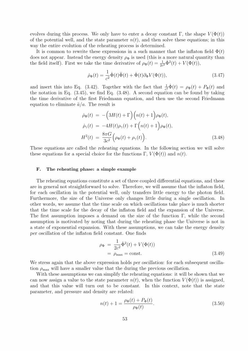
evolves during this process. We only have to enter a decay constant Γ, the shape V (Φ(t))of the potential well, and the state parameter n(t), and then solve these equations; in thisway the entire evolution of the reheating process is determined.

It is common to rewrite these expressions in a such manner that the inflaton field Φ(t)does not appear. Instead the energy density ρΦ is used (this is a more natural quantity thanthe field itself). First we take the time derivative of ρΦ(t) = 1

2c2Φ2(t) + V (Φ(t)),

ρΦ(t) =1

c2Φ(t)Φ(t) + Φ(t)∂ΦV (Φ(t)), (3.47)

and insert this into Eq. (3.42). Together with the fact that 1c2

Φ(t) = ρΦ(t) + PΦ(t) andthe notation in Eq. (3.45), we find Eq. (3.48). A second equation can be found by takingthe time derivative of the first Friedmann equation, and then use the second Friedmannequation to eliminate a/a. The result is

ρΦ(t) = −(

3H(t) + Γ)(n(t) + 1

)ρΦ(t),

ργ(t) = −4H(t)ργ(t) + Γ(n(t) + 1

)ρΦ(t),

H2(t) =8πG

3c2

(ρΦ(t) + ργ(t)

). (3.48)

These equations are called the reheating equations. In the following section we will solvethese equations for a special choice for the functions Γ, V (Φ(t)) and n(t).

F. The reheating phase: a simple example

The reheating equations constitute a set of three coupled differential equations, and theseare in general not straightforward to solve. Therefore, we will assume that the inflaton field,for each oscillation in the potential well, only transfers little energy to the photon field.Furthermore, the size of the Universe only changes little during a single oscillation. Inother words, we assume that the time scale on which oscillations take place is much shorterthat the time scale for the decay of the inflaton field and the expansion of the Universe.The first assumption imposes a demand on the size of the function Γ, while the secondassumption is motivated by noting that during the reheating phase the Universe is not ina state of exponential expansion. With these assumptions, we can take the energy densityper oscillation of the inflaton field constant. One finds

ρΦ =1

2c2Φ2(t) + V (Φ(t))

= ρmax = const. (3.49)

We stress again that the above expression holds per oscillation: for each subsequent oscilla-tion ρmax will have a smaller value that the during the previous oscillation.

With these assumptions we can simplify the reheating equations: it will be shown that wecan now assign a value to the state parameter n(t), when the function V (Φ(t)) is assigned,and that this value will turn out to be constant. In this context, note that the stateparameter, and pressure and density are related:

n(t) + 1 =ρΦ(t) + PΦ(t)

ρΦ(t). (3.50)

53

The assumption that the oscillations of the inflaton field are fast, allows us to replacenumerator and denominator by their averages over a single oscillation. Such an average< f(t) > is defined as an integral over all values that a function f(t) takes during theoscillation, divided by the period T of the oscillation,

< f(t) > ≡ 1

T

∫ T

0

f(t)dt. (3.51)

Since all time dependence is now integrated out, the expression for the state parametern(t) will yield a constant; this leads to a considerable simplification in solving the reheatingequations!

Before proceeding, we first need to calculate the time averages (3.50). This appears topresent a problem: to calculate the integrals, we need the functions ρΦ(t) and PΦ(t), andthese are precisely the functions we are trying to dfind by solving the reheating equations.However, there is a way out: we can rewrite the time-integrals in integrals over the inflatonfield, and we know that the inflaton field oscillates between two extreme values,

Φ0 ≡ Φ(t = 0), and Φ1/2 ≡ Φ(t =T

2). (3.52)

Here, Φ0 is the value of the inflaton field when it starts the oscillation: it is the value of thefield at the top of the well. The second is the value the inflaton field assumes when it ishalfway the oscillation: it is the magnitude of the field when it is at the bottom of the well,and when it starts increasing again.

It turns out that this information is sufficient for calculating the integrals. The averagescan be written as

< f(t) > ≡ 1

T

∫ T

0

f(t)dt =2

T

∫ Φ1/2

Φ0

f(t)

Φ(t)dΦ. (3.53)

By assuming that the energy density of the field is constant during a single oscillation, itfollows that

ρΦ =1

2c2Φ2(t) + V (Φ(t)) = ρmax → Φ(t) = ±

√2c2(ρmax − V (Φ(t))

), (3.54)

and we can write the average < f(t) > as

< f(t) >= ± 2

T

∫ Φ1/2

Φ0

f(t)(

2c2(ρmax − V (Φ(t))

))−1/2

dΦ. (3.55)

This is a useful expression. By inserting the general expressions for the energy density andpressure due to the inflaton field, we find that the numerator and denominator of Eq. (3.50)can be written as

<(ρΦ(t) + pΦ(t)

)> = ± 2

T

√2c2ρmax

∫ Φ1/2

Φ0

(1− V (Φ(t))

ρmax

)1/2

dΦ,

< ρΦ(t) > = ± 2

T

√ρmax2c2

∫ Φ1/2

Φ0

(1− V (Φ(t))

ρmax

)−1/2

dΦ. (3.56)

54

The state parameter n(t) is given by

n(t) + 1 =2c2∫ Φ1/2

Φ0

(1− V (Φ)

ρmax

)1/2

dΦ∫ Φ1/2

Φ0

(1− V (Φ)

ρmax

)−1/2

dΦ

. (3.57)

What remains to be done is to insert the specific shape V (Φ(t)) for the potential well inwhich the inflaton field oscillates, and the values Φ0 and Φ1/2 the inflaton field assumes atthe lowest and highest point in the well.

Next, we choose a specific well and calculate the state parameter. When this is accom-plished, it is only a small step to solve the reheating equations. As a follow up to theprevious example, we again consider the case of a massive inflaton field. As we have seenbefore, the potential energy density can be written as

V (Φ(t)) =m2

2

( c~

)2

Φ2(t), (3.58)

where m represents the mass of the inflatons. This function defines a parabolic well, withat the lowest point Φ = 0. Thus, at the bottom of this well,

Φ1/2 = 0. (3.59)

To determine the value of Φ0, we need to consider that when the inflaton is just startingan oscillation, it has not yet obtained kinetic energy density, Φ = 0, and the resulting totalenergy density is given entirely by the potential energy density. One finds

ρΦ = V (Φ) =m2

2

( c~

)2

Φ20. (3.60)

We assumed that the total energy density was constant during a single oscillation, ρΦ = ρmax,and we find for the value of the inflaton field at the highest point in the well

Φ0 = ±

√2ρmaxm2

(~c

)2

. (3.61)

Next, we evaluate the integrals in de numerator and denominator of Eq. (3.57). When weenter the potential well given by Eq. (3.58), the denominator is given by∫ Φ1/2

Φ0

(1− 1

ρmax

m2

2

( c~

)2

Φ2)−1/2

dΦ. (3.62)

To simplify our notation, we will introduce a variable x, for which

x ≡ m√2ρmax

( c~

)Φ. (3.63)

The integral in Eq. (3.62) already appears more friendly. We find

√2ρmaxm

(~c

)∫ 0

1

(1− x2

)−1/2

dx. (3.64)

55

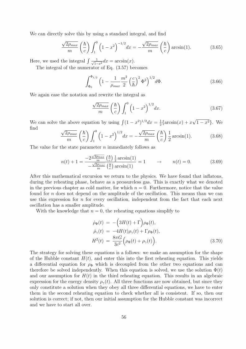
We can directly solve this by using a standard integral, and find

√2ρmaxm

(~c

)∫ 0

1

(1− x2

)−1/2

dx = −√

2ρmaxm

(~c

)arcsin(1). (3.65)

Here, we used the integral∫

1√1−x2dx = arcsin(x).

The integral of the numerator of Eq. (3.57) becomes∫ Φ1/2

Φ0

(1− 1

ρmax

m2

2

( c~

)2

Φ2)1/2

dΦ. (3.66)

We again ease the notation and rewrite the integral as

√2ρmaxm

(~c

)∫ 0

1

(1− x2

)1/2

dx. (3.67)

We can solve the above equation by using∫

(1 − x2)1/2dx = 12arcsin(x) + x

√1− x2. We

find √2ρmaxm

(~c

)∫ 0

1

(1− x2

)1/2

dx = −√

2ρmaxm

(~c

)1

2arcsin(1). (3.68)

The value for the state parameter n immediately follows as

n(t) + 1 =−2√

2ρmaxm

(~c

)12

arcsin(1)

−√

2ρmaxm

(~c

)arcsin(1)

= 1 → n(t) = 0. (3.69)

After this mathematical excursion we return to the physics. We have found that inflatons,during the reheating phase, behave as a pressureless gas. This is exactly what we denotedin the previous chapter as cold matter, for which n = 0. Furthermore, notice that the valuefound for n does not depend on the amplitude of the oscillation. This means than we canuse this expression for n for every oscillation, independent from the fact that each nextoscillation has a smaller amplitude.

With the knowledge that n = 0, the reheating equations simplify to

ρΦ(t) = −(

3H(t) + Γ)ρΦ(t),

ργ(t) = −4H(t)ργ(t) + ΓρΦ(t),

H2(t) =8πG

3c2

(ρΦ(t) + ργ(t)

). (3.70)

The strategy for solving these equations is a follows: we make an assumption for the shapeof the Hubble constant H(t), and enter this into the first reheating equation. This yieldsa differential equation for ρΦ which is decoupled from the other two equations and cantherefore be solved independently. When this equation is solved, we use the solution Φ(t)and our assumption for H(t) in the third reheating equation. This results in an algebraicexpression for the energy density ργ(t). All three functions are now obtained, but since theyonly constitute a solution when they obey all three differential equations, we have to enterthem in the second reheating equation to check whether all is consistent. If so, then oursolution is correct; if not, then our initial assumption for the Hubble constant was incorrectand we have to start all over.

56

What would be a good assumption for H(t)? We can imagine the following: at the startof the reheating phase the only significant form of energy density arises from the inflatonfield. We have seen that it behaves as cold matter. According to our calculations thecorresponding Hubble constant equals H(t) = 2

3t. After the inflaton field has decayed to

photons, the energy density due to radiation dominates that from inflatons. This density ischaracterized by a Hubble constant equal to H(t) = 1

2t. Consequently, it seems reasonable to

choose a function H(t) that for small t equals H(t) = 23t

, and for increasing t asymptotically

approaches H(t) = 12t

. In principle, an infinite amount of functions can be found which obeythese demands, and we choose the following as an example:

H(t) =1

t

(1

2+

1

6e−αt

). (3.71)

We could insert this function and then (perhaps) discover whether we have the correctdescription. This is certainly not the case for our chosen function. A solution of the inflationequations has not yet been found and we still do not know the time evolution of the energydensities ρΦ, ργ and the scale factor a(t). However, we are in fact not so interested in thedetailed time evolution. All we want to know is whether our model yields the correct amountof photons, such that the Standard Model can take over the evolution of Universe. To obtaina satisfactory answer to this question we only need an approximate solution of the reheatingequations (3.70). This is much easier than finding a complete solution.

The strategy is a follows. We split the problem into two parts: first we consider the timeevolution at the start of the reheating phase, thus in the time domain where the inflatonfield dominates the energy density, and find approximate solutions. Subsequently, we willconsider the end of the reheating phase, the time domain where photons dominate the energydensity, and obtain approximate solutions. In doing this we will also find the time ttransition

where the energy density due to photons overtakes that due to inflatons. The solutions willcontain a number of free constants, and we will assign values to these by demanding thatthe solutions from the different time domains smoothly join at ttransition. In this manner wefind functions ρΦ, ργ and a(t), that approximately solve the reheating equations.

First, we consider the time domain where the energy density due to inflatons dominates:

ρΦ ργ. (3.72)

In this region the Hubble constant is given by H(t) = 23t

, and we write the third reheatingequation as

4

9t2=

8πG

3c2ρΦ. (3.73)

An expression for the energy density of the inflaton field immediately follows,

ρΦ(t) =3c2

8πG

4

9t2. (3.74)

We substitute this into the first reheating equations, and find

− 8

9t23c2

8πG= −

(2

t+ Γ

) 3c2

8πG

4

9t2, (3.75)

and this can only be true when

Γ 2

t. (3.76)

57

The above states that our solution, see Eq. (3.78), is only valid for times smaller thant ≈ Γ−1. this is what we expect: surely, when the inflaton field rapidly decays to photons(thus when Γ is large), then soon (at t = Γ−1) the energy density ρΦ is smaller than ργ.The expression found for ρΦ can now be inserted into the second reheating equation, andthis yields a differential equation for the energy density ργ due to photons. One finds

ργ(t) = − 8

3tργ + Γ

3c2

8πG

4

9t2. (3.77)

The solution is given by

ργ(t) =1

t2

(ργ<t2/3

+12t

45

3c2

8πGΓt). (3.78)

Here, ργ< is a free constant. Its value can be found with the help of the following argument:during inflation all energy density due to normal matter and radiation vanishes. Therefore,we demand that during the reheating phase (this means: at the end of inflation) the energydensity ργ vanishes. Inflation ended at instant tend, given in Eq. (3.36); when we insert thisin Eq. (3.78) and demand that the result vanishes, we obtain for the constant ργ<

ργ< = −12

45Γ

3c2

8πG

(3~mc4

√8πG

6Φ0

)5/3

. (3.79)

With this the entire solution is known! At the start of the reheating phase H(t), ρΦ(t) andργ(t) are given by

H(t) =2

3t,

ρΦ(t) =3c2

8πG

4

9t2,

ργ(t) =1

t2

(− 12

45Γ

3c2

8πG

( 3~mc4

√8πG

6Φ0

)5/3 1

t2/3+

12t

45

3c2

8πGΓt

). (3.80)

This solution only holds for times t Γ−1.The second step in our analysis involves solving the reheating equations for times where

the photon density exceeds the density due to inflatons. Then

ργ ρΦ. (3.81)

The Hubble constant is now given by H(t) = 12t

, and the third reheating equation

1

4t2=

8πG

3c2ργ. (3.82)

The expression for the energy density ργ(t) directly follows,

ργ(t) =3c2

8πG

1

4t2. (3.83)

Next, we use the expression for the Hubble constant to express the first reheating equationas

ρΦ(t) = −( 3

2t+ Γ

)ρΦ(t). (3.84)

58

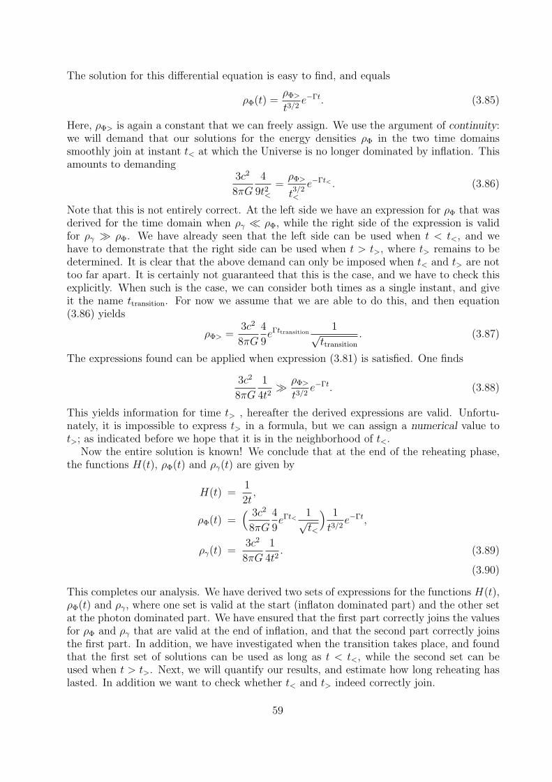
The solution for this differential equation is easy to find, and equals

ρΦ(t) =ρΦ>

t3/2e−Γt. (3.85)

Here, ρΦ> is again a constant that we can freely assign. We use the argument of continuity:we will demand that our solutions for the energy densities ρΦ in the two time domainssmoothly join at instant t< at which the Universe is no longer dominated by inflation. Thisamounts to demanding

3c2

8πG

4

9t2<=ρΦ>

t3/2<

e−Γt< . (3.86)

Note that this is not entirely correct. At the left side we have an expression for ρΦ that wasderived for the time domain when ργ ρΦ, while the right side of the expression is validfor ργ ρΦ. We have already seen that the left side can be used when t < t<, and wehave to demonstrate that the right side can be used when t > t>, where t> remains to bedetermined. It is clear that the above demand can only be imposed when t< and t> are nottoo far apart. It is certainly not guaranteed that this is the case, and we have to check thisexplicitly. When such is the case, we can consider both times as a single instant, and giveit the name ttransition. For now we assume that we are able to do this, and then equation(3.86) yields

ρΦ> =3c2

8πG

4

9eΓttransition

1√ttransition

. (3.87)

The expressions found can be applied when expression (3.81) is satisfied. One finds

3c2

8πG

1

4t2 ρΦ>

t3/2e−Γt. (3.88)

This yields information for time t> , hereafter the derived expressions are valid. Unfortu-nately, it is impossible to express t> in a formula, but we can assign a numerical value tot>; as indicated before we hope that it is in the neighborhood of t<.

Now the entire solution is known! We conclude that at the end of the reheating phase,the functions H(t), ρΦ(t) and ργ(t) are given by

H(t) =1

2t,

ρΦ(t) =( 3c2

8πG

4

9eΓt<

1√t<

) 1

t3/2e−Γt,

ργ(t) =3c2

8πG

1

4t2. (3.89)

(3.90)

This completes our analysis. We have derived two sets of expressions for the functions H(t),ρΦ(t) and ργ, where one set is valid at the start (inflaton dominated part) and the other setat the photon dominated part. We have ensured that the first part correctly joins the valuesfor ρΦ and ργ that are valid at the end of inflation, and that the second part correctly joinsthe first part. In addition, we have investigated when the transition takes place, and foundthat the first set of solutions can be used as long as t < t<, while the second set can beused when t > t>. Next, we will quantify our results, and estimate how long reheating haslasted. In addition we want to check whether t< and t> indeed correctly join.

59

We continue our example, and again take a mass m for the inflaton, while the constantΦ0 is given by

m ≈ 1013 GeV

c2≈ 10−14 kg, and Φ0 ≈ 1023

√m · kg

s. (3.91)

For the decay constant Γ we assume

Γ ≈ 1032 s−1. (3.92)

How did we obtain this value? It is an assumption! The constant Γ was introduced asa measure for the decay rate of inflatons (through some chain particle decay) to photons.Only little is known about the manner in which inflatons are coupled to other particles, andit is speculative to assume a value for the decay rate. However, there is a general rule inquantum field theory that states that more massive particles decay faster to other particles.We choose Γ proportional to m and state

Γ ≈ mc2

~. (3.93)

(both sides now have units 1/s). With this assumption we can calculate the times t< andt>. The first value is found by solving Eq. (3.76), and the second by solving Eq. (3.88). Wefind

t< ≈ 10−32 s, and t> ≈ 10−32 s. (3.94)

These values are (to the extend that our approximations can tell the difference) identical, andwe denote the transition point as ttransition. After this time the inflaton field has transferredsufficient energy to the photon field, that the Universe is radiation dominated. The constantρΦ> is fixed by Eq. (3.87) as

ρΦ> ≈ 1042 kg

m√

s. (3.95)

Now all constants are determined, and the evolution of the reheating phase is known. Forall times between the end of inflation, tend, and the transition point ttransition we can use Eqs.(3.80) and for times after the transition we use Eqs. (3.90). After the Universe has becomedominated by radiation, the Standard Model can be used to describe the evolution. Thetransition time is the time when the reheating phase ended: in our model reheating lastedabout 10−32 seconds.

60

IV. RELATIVISTIC STARS

A. Spherically symmetric stars

Strong gravitational fields exist not only in cosmology near the initial singularity, butalso in the interior of very dense stars and black holes. In this section, for simplicity weconsider only idealized stars that are spherically symmetric and static, i.e., unchanging.

The requirements of spherical symmetry and staticity imply that 4-dimensional spacetimecan be sliced into 3-dimensional spatial hypersurfaces which all have the same geometry; andthese are in turn built out of 2-dimensional concentric spheres. The most general sphericallysymmetric, static spacetime has line element

ds2 = −e2Φdt2 + e2Λdr2 + r2(dθ2 + sin2 θdφ2) (4.1)

= −e2Φdt2 + e2Λdr2 + r2dΩ2, (4.2)

where for brevity we have introduced

dΩ2 = dθ2 + sin2 θdφ2. (4.3)

The flat Minkowski metric has Φ = Λ = 0. In general, Φ and Λ will be functions of r – butnot of t (because of staticity) or θ, φ (because of spherical symmetry).

We will want to solve the Einstein equations for the line element (4.2). A straighforwardcalculation shows that the Einstein tensor has components

G00 =1

r2e2Φ d

dr

[r(1− e−2Λ)

], (4.4)

Grr = − 1

r2e2Λ(1− e−2Λ) +

2

rΦ′, (4.5)

Gθθ = r2e−2Λ

[Φ′′ + (Φ′)2 +

Φ′

r− Φ′Λ′ − Λ′

r

], (4.6)

Gφφ = sin2 θGθθ, (4.7)

with ′ = d/dr, and all other components vanish.We will also need to specify an energy-momentum tensor for the matter our idealized

stars are made of. Any fluid in thermodynamical equilibrium has an equation of state of theform

P = P (ρ, S) (4.8)

which relates the pressure to the energy density ρc2 and the specific entropy S. In manycases the dependence on S can be neglected (e.g., because the latter is negligibly small andcan be considered zero), and this is what we do here:

P = P (ρ). (4.9)

For a perfect fluid with density ρ and pressure P one has

T µν = (ρ+ P )UµUν + Pgµν , (4.10)

where Uµ is the 4-velocity of the fluid. The latter must satisfy

UµUµ = UµUνgµν = −1, (4.11)

61

and if the star is to be static it can only have a t component. This implies

U0 = e−Φ, U0 = eΦ (4.12)

with all other components zero. The energy-momentum tensor has components

T00 = ρ e2Φ, (4.13)

Trr = P e2Λ, (4.14)

Tθθ = r2P, (4.15)

Tφφ = sin2 θ Tθθ. (4.16)

This has to satisfy the conservation law

∇µTµν = 0. (4.17)

Because of the high degree of symmetry, the only one of these equations that is non-vanishingis the one where ν = r. It takes the form

(ρ+ P )dΦ

dr= −dP

dr. (4.18)

This equation tells us what pressure gradient is needed to keep the fluid static in the grav-itational field, whose effect depends on dΦ/dr.

The (0, 0) component of the Einstein equations can be found from Eqns. (4.4) and (4.13).At this point it is convenient to introduce the function

m(r) =1

2r (1− e−2Λ(r)), (4.19)

so that

grr = e2Λ =1

1− 2m(r)r

. (4.20)

Then the (0, 0) Einstein equation implies

dm(r)

dr= 4πr2ρ(r). (4.21)

This is exactly what one would obtain in Newtonian theory if m(r) were the mass enclosedby the radius r. This interpretation is not tenable here, as we shall see in a moment;nevertheless m(r) is convenient to calculate with.

The (r, r) Einstein equation can be found from Eqns. (4.5) and (4.14); it can be put inthe form

dΦ

dr=m(r) + 4πr2P

r [r − 2m(r)]. (4.22)

We now in turn discuss the exterior solution where ρ = P = 0, and possible interiorsolutions which depend on the details of the equation of state P = P (ρ).

62

B. Exterior solution

Outside the star we have ρ = P = 0, and the Einstein equations (4.21) and (4.22) reduceto

dm

dr= 0, (4.23)

dΦ

dr=

m

r(r − 2m). (4.24)

These have the solutions

m(r) = M = const, (4.25)

e2Φ(r) = 1− 2M

r, (4.26)

where we have assumed Φ→ 0 as r →∞, as is required if the spacetime is to be asymptot-ically flat (i.e., if we move sufficiently far from the center we recover Minkowski spacetime).One has

M = m(R), (4.27)

where r = R is the coordinate radius of the star’s surface. It follows that the exteriorspacetime has the following form:

ds2 = −(

1− 2M

r

)dt2 +

1

1− 2Mr

dr2 + r2dΩ2. (4.28)

This is the Schwarzschild metric.Using the geodesic equation, one can show (see below) that at sufficiently large distances

and restoring G, a test particle will feel a purely radial inward acceleration ar = −GM/r2.This justifies the choice of the symbol M : it is the mass the star is perceived to have a largedistance away. However, it is not the proper mass of the star. The latter would be

Mp =

∫ √(3)g ρ d3x (4.29)

= 4π

∫ R

0

ρ(r)

[1− 2m(r)

r

]−1/2

r2dr, (4.30)

where we used the proper volume element on a t = 0 hypersurface,√

(3)g d3x. By contrast,from (4.21) one simply has

M = 4π

∫ R

0

ρ(r) r2dr. (4.31)

Clearly M < Mp, the difference being due to the gravitational binding energy.Although we have not shown it, Birkhoff’s theorem says that the metric (4.28) is the

only spherically symmetric and asymptotically flat solution of the vacuum Einstein equa-tions, even if one drops the requirement that the spacetime be static! In particular, theexterior spacetime of a spherically symmetric star that is pulsating only radially is neces-sarily Schwarzschild. We will make use of Birkhoff’s theorem later on, when studying anexample of a star undergoing radial collapse to form a black hole.

63

C. Interior solution

Inside the star (r < R) one has, in general, ρ 6= 0 and P 6= 0. Dividing Eq. (4.18) by(ρ + P ) and using it to eliminate dΦ/dr in (4.24), one obtains the Tolman-Oppenheimer-Volkoff (TOV) equation:

dP

dr= −(ρ+ P ) (m+ 4πr3P )

r (r − 2m). (4.32)

The TOV equation, together with Eq. (4.21) and (4.9) are sufficient to solve for m(r),ρ(r), and P (r). The first two are first-order differential equations, requiring two integrationconstants. It is reasonable to set m(r = 0) = 0. The other constant, Pc = P (r = 0), isthe central pressure. Thus, given an equation of state, the latter completely determinesthe stellar model. Once we know m(r), ρ(r), and P (r), we can define the surface of thestar as the radius R where P (R) = 0 – notice that by the TOV equation, P (r) decreasesmonotonically. This radius R then determines M through M = m(R).

We now further simplify the treatment by positing

ρ = const, (4.33)

which replaces the equation of state (4.9). In a normal star this is not an appropriateassumption, but it is approximately true in the case of a neutron star. With this ansatz,Eq. (4.21) can be integrated immediately to give

m(r) =4πr3

3ρ. (4.34)

This is of course only valid for r < R; outside the star we have

M =4πR3

3ρ, (4.35)

so that M is now set by ρ and R. The TOV equation (4.32) becomes

dP

dr= −4

3πr

(ρ+ P ) (ρ+ 3P )

1− 8πr2ρ/3. (4.36)

Integrating from an arbitrary central density Pc we get

ρ+ 3P

ρ+ P=ρ+ 3Pcρ+ Pc

(1− 2m

r

)1/2

. (4.37)

It follows that the radius R is given by

R2 =3

8πρ

[1−

(ρ+ Pcρ+ 3Pc

)2], (4.38)

or

Pc = ρ1− (1− 2M/R)1/2

3(1− 2M/R)1/2 − 1. (4.39)

64

Substituting this into (4.37) one gets

P = ρ(1− 2Mr2/R3)1/2 − (1− 2M/R)1/2

3 (1− 2M/R)1/2 − (1− 2Mr2/R3)1/2. (4.40)

Using (4.18) we can now solve for Φ. In this case we know the value at r = R, since

g00(R) = −(1−M/R). (4.41)

Hence

eΦ(r) =3

2(1− 2M/R)1/2 − 1

2(1− 2Mr2/R3)1/2. (4.42)

This completes our derivation of the interior geometry in the constant density case.Notice that there is something peculiar about Eq. (4.39): as M/R → 4/9, Pc → ∞.

Given a mass M , a uniform density star can not have radius R ≤ 9M/4 or an infinitepressure would be needed to support it. It was shown by Buchdahl that this is true for anyspherically symmetric star model, assuming only that ρ ≥ 0 and dρ/dr ≤ 0, irrespective ofthe equation of state. If one constructs a star of R = 9M/4 and gives it a small radial pushinwards, it must collapse onto itself. The radius will become smaller and smaller, leavingnothing but Schwarzschild spacetime. This process is called complete gravitational collapse,and it results in the formation of a black hole.

The most common ultra-compact objects are not black holes but white dwarfs, whichform when ordinary stars run out of fuel and fusion processes stop. Electron degeneracy(as a consequency of the Pauli exclusion principle) then provides the pressure to sustain thestar. A typical white dwarf is thought to have a mass M of about a solar mass (M) anda radius comparable to that of Earth, in the order of 104 km. More generally, the radius Rscales like M−3. The largest mass (and hence the largest compactness) which the degenerateelectron gas can sustain is about 1.4 M (the Chandrasekhar limit).

Supernova explosions can produce objects that have a similar mass but are much morecompact: neutron stars, in which almost all electrons have combined with protons to leaveneutrons. Typical neutron stars have masses between 1.35 M and 2.1 M. The radius isdetermined by the equation of state, which is highly uncertain,24 but ∼ 10 km should betypical. Despite the uncertainties, 5 M is generally taken to be the largest neutron starmass that can be sustained. Though rare, there are main sequence stars of sufficient massto produce a remnant of neutron star size but heavier than 5 M when going supernova.There is no known physical process that would stop such an object to collapse into a blackhole.

24 In fact, gravitational wave signals from the coalescence of two neutron stars, which are expected to beobserved within the next 5 years or so, will be the one sure way to determine the equation of state of bulknuclear matter.

65

V. BLACK HOLES

We have seen that the exterior (vacuum) part of the spacetime of a spherically symmetric,static star is the Schwarzschild spacetime, Eq. (4.28):

ds2 = −(

1− 2M

r

)dt2 +

(1− 2M

r

)−1

dr2 + r2dΩ2. (5.1)

We also noted that if the radius R must satisfy R > 9M/4 in order that the density atthe center of the star remain finite. If R ≤ 9M/4 then the star cannot remain static andmust collapse. However, if the collapse happens in a spherically symmetric way, then theoutside, vacuum part of spacetime must remain Schwarzschild, as this is the only sphericallysymmetric and asymptotically flat solution to the vacuum Einstein equations. Followingcomplete gravitational collapse, (4.28) is what the remaining spacetime geometry looks like.

The way to understand the structure of a spacetime is to study the paths followed bymassless particles (e.g., photons) and by massive particles: null and timelike geodesics,respectively.

A. Conserved quantities

Given that the metric (5.1) has a large amount of symmetry, our task will be simplifiedgreatly by considering constants of the motion. Consider the geodesic equation:

uµ∇µuν = 0 (5.2)

with uµ the 4-velocity. Since ∇µgνρ = 0, we can lower the free index, so

uµ∇µuν = 0. (5.3)

If the geodesic is timelike (the spacetime path of a massive particle), uµ∂µ = d/dτ with τthe proper time; in the case of a null geodesic (the path of a photon), uµ∂µ = d/dλ, with λsome affine parameter. For a particle, Eq. (6.27) can be written as

duνdτ

= Γρµνuµuρ. (5.4)

Observe that

Γρµνuµuρ =

1

2gρσ(∂µgσν + ∂νgµσ − ∂σgµν)uµuρ

=1

2(∂µgσν + ∂νgµσ − ∂σgµν) gρσuρuµ

=1

2(∂µgσν + ∂νgµσ − ∂σgµν)uσuµ. (5.5)

The product uσuµ is symmetric in σ and µ, but the first and third terms inside the bracketsare together asymmetric in these indices; hence they cancel and we are left only with themiddle term:

Γρµνuµuρ =

1

2∂νgµσu

µuσ. (5.6)

66

We see that the geodesic equation can be written as

duνdτ

=1

2∂νgµσu

µuσ. (particles) (5.7)

The same goes for a null geodesic with the replacement of τ by the affine parameter λ. Thisleads to an important result: if all the components gµσ are independent of xν for a particularindex ν, then ∂νgµσ = 0, and uν is constant along the entire geodesic: it is a constant of themotion.

In the Schwarzschild metric (4.28), all metric components are independent of t, hence u0

is a constant of the motion. It is convenient to introduce another constant E:

E ≡ −u0. (5.8)

Note that in the case of a massive particle, u0 = p0/m with pµ the 4-momentum and m therest mass; E is then the energy per unit rest mass. In the case of a photon, E is simplythe energy. The metric is also independent of the angle φ, meaning uφ is a constant of themotion. We define

L ≡ uφ, (5.9)

where for a massive particle L is the orbital angular momentum per unit rest mass. Becauseof spherical symmetry, the motion will be confined to a plane. Without loss of generality wecan take this to be the equatorial plane, θ = π/2, and one then has uθ = dθ/dλ = 0, withλ any affine parameter along the orbit. The non-zero components of the 4-velocity uµ arethen

u0 = g0νuν = g00u0 = m

(1− 2M

r

)−1

E,

ur =dr

dτ,

uθ = 0,

uφ = gφνuν = gφφuφ =1

r2L. (5.10)

B. Elliptical and circular orbits

We can now use the defining equations for massive particles and photons:

massive particle: uµuµ = −1; photon: uµuµ = 0, (5.11)

oruµuν = −κ (5.12)

where κ = 1 for a massive particle and κ = 0 for a photon. When applied to our case, thisyields:

−E2

(1− 2M

r

)−1

+

(1− 2M

r

)−1(dr

dτ

)2

+L2

r2= −κ. (5.13)

This equality immediately gives us the equations for the radial part of the orbital motion;rewriting it slightly we have

1

2

(dr

dτ

)2

+1

2

(1− 2M

r

)(L2

r2+ κ

)=

1

2E2, (5.14)

67

Now introduce the effective potential

Veff (r) ≡1

2

(1− 2M

r

)(L2

r2+ κ

). (5.15)

Then the equation for radial motion (5.14) becomes

1

2

(dr

dτ

)2

+ Veff (r) =1

2E2. (5.16)

This is uncannily similar to what one gets in Newtonian gravity, where the radial motion isthe same as that of a particle with unit mass moving along a line, with total energy E2/2and experiencing an effective potential. In fact, let us make an explicit comparison. In GR,the particle has an effective potential

Veff (r) =1

2κ− M

rκ+

L2

2r2− ML2

r3. (5.17)

The first term is an irrelevant constant. The second term is the usual Newtonian potential.The third term also arises in the effective potential in Newtonian theory; it is the usual“centrifugal barrier term”. What is new is the third term, which is a new attractive termthat dominates the centrifugal barrier term at small r. It constitutes a crucial difference:As we will see in a moment, this term makes it impossible to have stable circular orbitsarbitrarily close to the center.

Let us first consider the trajectories of massive particles (κ = 1). Circular orbits (i.e.,orbits with dr/dτ = 0) are given by extrema of the effective potential:

0 =dVeffdr

=Mr2 − L2r + 3ML2

r4, (5.18)

which has roots

R± =L2 ± (L4 − 12L2M2)1/2

2M. (5.19)

We see that if L2 < 12M2 there are no extrema; the particle has insufficient angularmomentum to be on a circular orbit and will fall inwards.

For L2 > 12M2, one can check that the extremum R+ is a minimum of V (r), while R− isa maximum; see Fig. 17. This means that for such values of the specific angular momentumL, there are two possible circular orbits (whereas in Newtonian gravity there would havebeen only one): a stable one at r = R+ and an unstable one at r = R−. It is not difficult tosee that R+ is restricted to the range

R+ > 6M, (5.20)

and R− is restricted to3M < R− < 6M. (5.21)

Thus, for a particle with mass, no stable circular orbits exist at r < 6M , and no circularorbits (stable or otherwise) exist for r < 3M . The last stable orbit (or innermost stablecircular orbit occurs when L2 = 12M2, in which case R+ = R− = 6M ; this is illustrated inFig. 18.

68

Figure 17: The effective potential for a massive particle with L2 = 24M2. The r coordinate isplotted in units of M . For comparison the Newtonian effective potential is also plotted (dashedline).

Figure 18: The effective potential for a massive particle with L2 = 12M2, the smallest angularmomentum for which there is a stable orbit (at r = 6M). By constrast, in Newtonian gravitystable orbits exist for arbitrarily small angular momentum.

69

Figure 19: The effective potential for a photon. There is an unstable circular orbit at r = 3M , butno stable orbits. The Newtonian effective potential consists of just the repulsive angular momentumterm; here there are never any circular orbits.

Repeating the above considerations for photons, we get

0 =dVeffdr

=−L2r + 3ML2

r4. (5.22)

In this case the only root isR = 3M, (5.23)

which is an unstable orbit; see Fig. (19). Thus, irrespective of angular momentum, the onlycircular orbit available to a photon is at r = 3M , but the tiniest perturbation will send itout to infinity or in towards the center. r = 3M is referred to as the light sphere.

What about the angular motion? Solving for L in the solution R+ of Eq. (5.19), one finds

L2 = Mr

(1− 3M

r

)−1

(5.24)

for the angular momentum of a massive particle on a stable circular orbit at coordinateradius r. Recalling that dr/dτ = 0 for circular orbits, one has E2 = 2Veff , hence

E2 =

(1− 2M

r

)2 (1− 3M

r

)−1

. (5.25)

Furthermore,

dφ

dτ= uφ = gφφL =

1

r2L, (5.26)

dt

dτ= u0 = g00(−E) =

(1− 2M

r

)−1

E. (5.27)

70

The angular velocity is then

dt

dφ=dt/dτ

dφ/dτ=

(r3

M

)1/2

=∆t

∆φ, (5.28)

where in the last equality we have used that dt/dφ is constant, as is evident from the next-to-last equality. The period P is the time ∆t taken to complete a revolution, i.e., ∆φ = 2π.This is given by

P = 2π

√r3

M. (5.29)

Formally, this is Kepler’s third law! However, the resemblance is superficial, because itrefers to the time coordinate t, which only corresponds to proper time τ as experienced byan observer for stationary observers at r →∞.

C. Radial infall

In the previous subsection we studied particles on circular orbits. What happens if aparticle falls radially inwards? From Eq. (5.14), we can integrate proper time. Up to anintegration constant,

τ =

∫dτ =

∫dr

[E2 − (1− 2M/r) (1 + L2/r2)]1/2. (5.30)

For a radially infalling particle, 0 = uφ = L/r2, hence L = 0. If the particle starts out withzero radial velocity at r = R then dr/dτ(r = R) = 0, or

E2 = 1− 2M

R. (5.31)

Substituting this in Eq. (5.30) and setting L = 0, we get

τ =

∫dr

[2M/r − 2M/R]1/2. (5.32)

Using this equation, it is possible to express the behavior of both r and τ in parametricform, namely

r =R

2(1 + cos η), (5.33)

τ =R

2

(R

2M

)1/2

(η + sin η). (5.34)

We see that η = 0 corresponds to r = R. When η = π, r = 0 so that the particle will havereached the center. In principle Eq. (5.33) could be continued by increasing η even further,but this would be incorrect, as we will discuss momentarily. From the above, it is clear thatthe particle hits the center after a finite proper time given by

∆τ =π

2R

(R

2M

)1/2

. (5.35)

71

What about coordinate time t? First note that

dr

dτ=dr

dt

dt

dτ=dr

dt

E

1− 2M/r. (5.36)

Combining this with Eq. (5.14) for dr/dτ , we can solve for dr/dt, or dt/dr. Again specializingto the case L = 0 and integrating, one finds

t =

∫dt =

∫E

[E2 − (1− 2M/r)]1/2dr

1− 2M/r. (5.37)

This integral is not easy, but it is possible to solve it analytically. We simply state the result(originally due to Khuri):

t =

[(R

2+ 2M

) (R

2M− 1

)1/2]η +

R

2

(R

2M− 1

)1/2

sin η

+2M ln

∣∣∣∣(R/2M − 1)1/2 + tan(η/2)

(R/2M − 1)1/2 − tan(η/2)

∣∣∣∣ , (5.38)

where η is the same parameter as before. We now notice something strange. The aboveexpression diverges for η = η where

tan(η/2) =

(R

2M− 1

)1/2

. (5.39)

With some trigonometry, this turns out to imply

cos(η) =4M

R− 1. (5.40)

However, from Eq. (5.33) we know that this implies r = 2M !

D. The Schwarzschild horizon

Let us take stock. Eqns. (5.33) and (5.34) describe the motion of an infalling particleas seen by an observer A moving along with that particle, who will have proper time τ .According to this observer, the particle will reach the center after a finite time given byEq. (5.35). An observer B who is stationary and at large distance (r → ∞) has a propertime that coincides with coordinate time t. According to observer B, the particle will neverreach the center; in fact, as t→∞, the particle’s radial position asymptotically approachesr = 2M .

Looking at the metric (5.1), one already suspects that the surface r = 2M is special;indeed, as r → 2M , g00 → 0 and grr → ∞. However, r = 2M is only a coordinatesingularity. The measurable quantities associated with the geometry of spacetime are notthe metric components, but the components of the Riemann tensor, as they determine tidalforces. Now, one can check that the components of Rµ

νρσ all remain finite as r → 2M .Hence the infinities in the metric are mere coordinate artefacts, which can be dealt with bychoosing a different coordinate system. We leave it as an exercise to find such coordinatesystems.

72

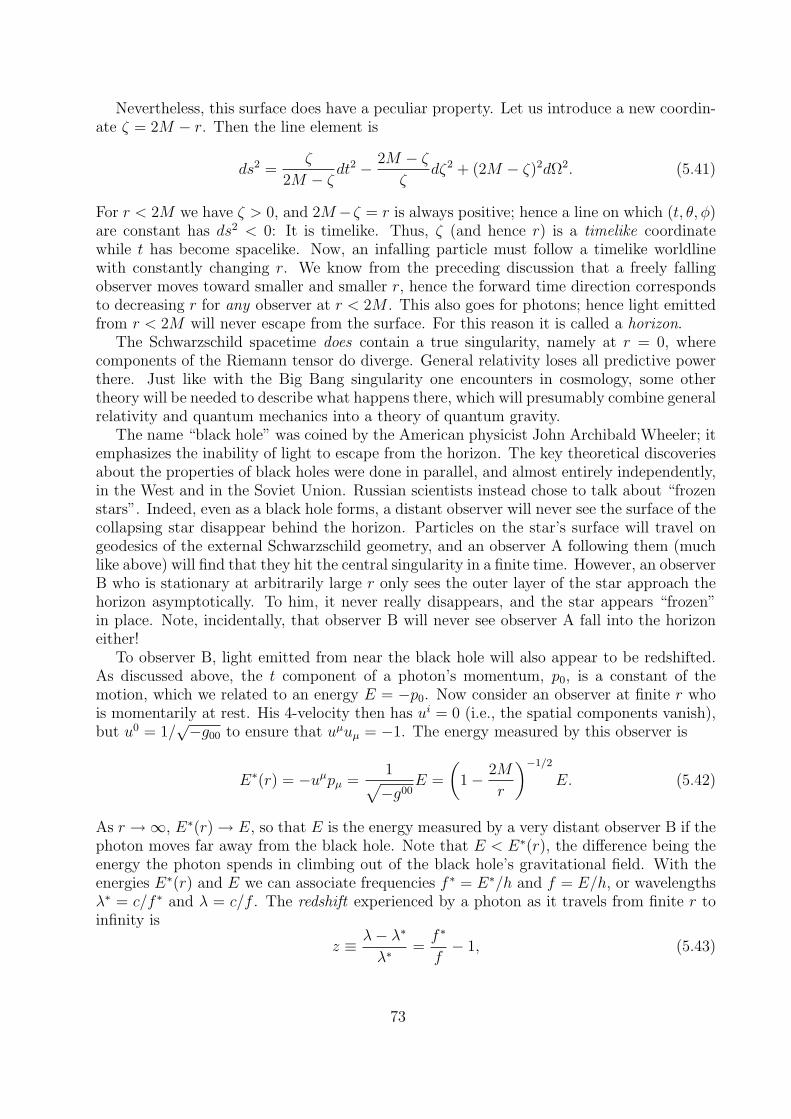
Nevertheless, this surface does have a peculiar property. Let us introduce a new coordin-ate ζ = 2M − r. Then the line element is

ds2 =ζ

2M − ζdt2 − 2M − ζ

ζdζ2 + (2M − ζ)2dΩ2. (5.41)

For r < 2M we have ζ > 0, and 2M−ζ = r is always positive; hence a line on which (t, θ, φ)are constant has ds2 < 0: It is timelike. Thus, ζ (and hence r) is a timelike coordinatewhile t has become spacelike. Now, an infalling particle must follow a timelike worldlinewith constantly changing r. We know from the preceding discussion that a freely fallingobserver moves toward smaller and smaller r, hence the forward time direction correspondsto decreasing r for any observer at r < 2M . This also goes for photons; hence light emittedfrom r < 2M will never escape from the surface. For this reason it is called a horizon.

The Schwarzschild spacetime does contain a true singularity, namely at r = 0, wherecomponents of the Riemann tensor do diverge. General relativity loses all predictive powerthere. Just like with the Big Bang singularity one encounters in cosmology, some othertheory will be needed to describe what happens there, which will presumably combine generalrelativity and quantum mechanics into a theory of quantum gravity.

The name “black hole” was coined by the American physicist John Archibald Wheeler; itemphasizes the inability of light to escape from the horizon. The key theoretical discoveriesabout the properties of black holes were done in parallel, and almost entirely independently,in the West and in the Soviet Union. Russian scientists instead chose to talk about “frozenstars”. Indeed, even as a black hole forms, a distant observer will never see the surface of thecollapsing star disappear behind the horizon. Particles on the star’s surface will travel ongeodesics of the external Schwarzschild geometry, and an observer A following them (muchlike above) will find that they hit the central singularity in a finite time. However, an observerB who is stationary at arbitrarily large r only sees the outer layer of the star approach thehorizon asymptotically. To him, it never really disappears, and the star appears “frozen”in place. Note, incidentally, that observer B will never see observer A fall into the horizoneither!

To observer B, light emitted from near the black hole will also appear to be redshifted.As discussed above, the t component of a photon’s momentum, p0, is a constant of themotion, which we related to an energy E = −p0. Now consider an observer at finite r whois momentarily at rest. His 4-velocity then has ui = 0 (i.e., the spatial components vanish),but u0 = 1/

√−g00 to ensure that uµuµ = −1. The energy measured by this observer is

E∗(r) = −uµpµ =1√−g00

E =

(1− 2M

r

)−1/2

E. (5.42)

As r →∞, E∗(r)→ E, so that E is the energy measured by a very distant observer B if thephoton moves far away from the black hole. Note that E < E∗(r), the difference being theenergy the photon spends in climbing out of the black hole’s gravitational field. With theenergies E∗(r) and E we can associate frequencies f ∗ = E∗/h and f = E/h, or wavelengthsλ∗ = c/f ∗ and λ = c/f . The redshift experienced by a photon as it travels from finite r toinfinity is

z ≡ λ− λ∗

λ∗=f ∗

f− 1, (5.43)

73

and one has

z =1√

1− 2M/r− 1. (5.44)

For a photon emitted close to the horizon, r = 2M+ε, the redshift becomes arbitrarily largeas ε→ 0.

E. Non-spherical black holes

So far we only considered spherically symmetric, asymptotically flat, vacuum black holes,in which case the Schwarzschild black hole is the only possible solution, as stated by Birk-hoff’s theorem.

However, one can also look for solutions to the Einstein equations that are sphericallysymmetric and asymptotically flat and contain not matter, but include an electromagneticfield. In special relativity one can write down an energy-momentum tensor for electro-magnetism, which generalizes to curved spacetimes by replacing coordinate derivatives withcoordinate derivatives. By using this energy-momentum tensor Tµν in the right hand side ofthe Einstein equations and again specializing to spherical symmetry and asymptotic flatness,once again a unique, static solution is arrived at, namely the Reissner-Nordstrom black hole.This is a black hole with an electric charge Q at r = 0, which causes an electric field thatpermeates space. These solutions are probably not very relevant in terms of astrophysics,because black holes are formed by the gravitational collapse of ordinary star remnants, whichto an excellent approximation are electrically neutral (Q = 0).

More interesting are cylindrically symmetric asymptotically flat black holes in vacuum(Tµν = 0 again), called Kerr-Newman black holes. These represent rotating black holes.Since no matter is involved, what is rotating is space itself. Rotating black holes are sur-rounded by an ergosphere, a region where it is not possible to stand still, and one needs tomove around the horizon in the direction of rotation of the hole; see Fig. 20. The rotationalpull of a rotating black hole (not only inside the ergosphere but also outside it) is calledframe dragging. The ergosphere has another peculiar property. When a particle enters itfrom the outside, then according to observers at large distances, its energy becomes negative.This leads to an interesting effect called the Penrose process. Suppose a particle is sent intothe ergosphere and made to break up into two particles. Imagine the break-up is arranged insuch a way that one particle falls into the horizon, while the other escapes to infinity. Sincethe particle falling in is adding negative energy to the black hole, the particle that escapeswill have a larger (positive) energy than the outgoing particle: energy has been extractedfrom the black hole. What happens is that part of the rotational kinetic energy of the blackhole is taken away. In principle the process can be repeated over and over again until all ofthe rotational energy is depleted, and one ends up with a non-rotating, Schwarzschild blackhole. Now suppose one measures the mass M of the black hole as by holding a particle withmass m at a large distance and looking at the force one needs to exert to keep it in its place(for r → ∞, simply F = −GMm/r2). Then as energy is extracted, M will decrease! Thisis because the rotational kinetic energy contributes to the measured M .

In principle, a rotating black hole can also have charge. However, in general relativity,

74

a stationary (possibly rotating), asymptotically flat black hole spacetime is completely de-termined by three numbers25: the mass M , the rotational angular momentum J , and theelectric charge Q. This is the Black Hole Uniqueness Theorem (also known as the No HairTheorem), and it leads to a strong test of GR. By tracking a small object that is closelyorbiting the horizon of a much larger black hole, one can tell from the orbit if the spacetimecan indeed be described by only three numbers; if not, then GR is wrong. So far it hasnot been possible to perform this test effectively, because the smaller object would itselfhave to be a black hole so that it can orbit sufficiently closely without breaking apart; butthen the object is not directly observable. However, later on we will talk about the futurespace-based gravitational wave observatory LISA, which will pick up gravitational radiation(ripples in the curvature of spacetime) emitted by precisely such systems. The details of thesmaller black hole’s orbit can be inferred from the gravitational wave signal it emits, andthis will enable high-accuracy tests of the Uniqueness Theorem.

Figure 20: In the case of rotating black holes, the horizon is surrounded by an ergosphere, a regionwhere it is not possible to stand still and one has to rotate along with the hole.

As indicated in Fig. 20, just like Schwarzschild black holes, rotating black holes havea horizon. However, this is only true if the angular momentum J satisfies J/M2 ≤ 1. IfJ/M2 > 1, then there is no horizon and one has a naked singularity. Computer simulationsof complete gravitational collapse of rotating clouds of matter have always led to a blackhole with a horizon, J/M2 ≤ 1. Penrose has conjectured that given some mild conditionson the kind of matter used (essentially positivity of the energy density), one will always endup with such a black hole; this is referred to as the Cosmic Censorship Conjecture. Quitepossibly, the conjecture can be proven as a theorem, in which case it too would be a necessaryconsequence of GR. If a naked singularity were part of a close binary system, then once againone would be able to infer this from the gravitational wave signal. If the conjecture is indeeda theorem, then finding a naked singularity would immediately invalidate GR.

25 Actually, one can also have black holes with, e.g., color charge as in quantum chromodynamics. Suchblack holes are of no astrophysical interest, although occasionally they are used in thought experiments.

75

F. Evidence for the existence of black holes

There is a great deal of (admittedly circumstantial) evidence for the existence of blackholes. Almost all of this evidence is for black holes in one of two categories:

1. Supermassive black holes have masses between 106 and 1010M. Most galaxies arebelieved to harbor a supermassive black hole in their centers, including our own.By tracking stars near the center of our galaxy over a period of years, it has beenestablished that a dark object with a mass of ∼ 4 × 106M is present there; seeFig. 21. The object is no larger than an AU (or Astronomical Unit, the radius of theEarth’s orbit around the Sun, which is about 1.5 × 108 km); for comparison, if it isindeed a black hole then its horizon has a size of 6× 106 km.

Figure 21: The orbits of stars in a region called Sagittarius A∗, near the center of the Milky Waygalaxy, indicate the presence of an object of about 4 million solar masses, confined to a region nowider than the Earth’s orbit around the Sun.

More evidence comes from Active Galactic Nuclei, galactic centers that emit copiousamounts of radiation. The source is believed to be an accretion disk surrounding ablack hole; the heating due to the compression of gas spiraling towards the center.Magnetic fields lining the accretion disk cause material to be ejected in tight jetsperpendicular to the disk. A black hole is the only known explanation given thesefeatures and the amount of energy involved. Ordinary galactic centers also exhibitjets, only much smaller than with AGNs, presumably because the black hole hasalready devoured most of the matter in its immediate vicinity. Fig. 22 shows a jetnear the center of M87.

76

Figure 22: A jet of material emitted by the center of the galaxy M87.

2. Stellar mass black holes with masses between three and a few tens M. These probablyfuel so-called X-ray binaries, where a stellar mass black hole and a normal star orbiteach other. The tug from the black hole rips material away from the star’s outerlayers, causing an accretion disk to form. There is evidence that the accretion disktends to have a well-defined inner edge, consistent with the existence of a last stableorbit. Of course, in the approximation of spherical symmetry, we have seen that inprinciple there can be stable stars with radius R > 9M/4 while the last stable orbithas a radius of 6M . However, if the dark object in an X-ray binary had a solid surface,then material crashing into it would cause radiation with a very different frequencydistribution than the radiation from an accretion disk. This is not seen, suggestingthe existence of a horizon.

Supermassive black holes may have come into being through successive mergers of muchsmaller black holes in the far past; alternatively, they could have been created almost inone go through the collapse of proto-galactic disks. LISA will see gravitational wave signalsfrom massive black holes out to redshifts z > 15 and will be able to clearly distinguishbetween the two formation mechanisms. One may wonder about the mass gap betweenthe supermassive and the stellar mass black holes. Holes with masses of, say, 104M arepresumed to be rare in the later epochs of the history of the Universe, as they should haveturned into supermassive black holes by then through accretion and mergers. It is possiblethat globular clusters, nearly spherical systems of stars that orbit the centers of galaxies, cangenerate intermediate mass black holes of hundreds to tens of thousands of M, althoughright now there is little evidence of this. Here too, gravitational wave detectors will havethe last word.

Note that the above evidence is indeed circumstantial. The existence of black holes willonly be settled definitively when we attain access to gravitational wave signals from a blackhole merging with another compact object.

77

VI. GRAVITATIONAL WAVES AND THEIR PROPERTIES

A. Dynamical gravity

In Newton’s theory of gravity, any changes in the distribution of matter, no matter howlocalized, are felt instantaneously at arbitrarily large distances. Despite the huge successesof Newton’s theory, this instantaneous action at a distance was considered unsatisfactoryalready by some of his contemporaries in the late 17th century. These tried to come upwith some dynamical mechanism through which the gravitational force would be commu-nicated, but without success. The issue became especially pressing after the development ofspecial relativity (1905), which imposes a strict speed limit, the speed of light, on how fastcommunication of any kind can be effected.

Maxwell’s theory of electromagnetism does not have this instantaneous action at a dis-tance. Consider a localized charge and/or current distribution (the “source”) causing electricand magnetic fields E and B. From the Maxwell equations it can be shown that at a time t,the values of E and B at a distance D from the source depend on what the source was doingat a time t−D/c. The time lag, D/c, is the time needed for a signal to cross the distanceD if it traveled at the speed of light: electromagnetism obeys Einstein’s speed limit. E andB can be shown to obey a wave equation: the changes in a charge/current distribution arecommunicated to the rest of space by electromagnetic waves. Thus, unlike the Newtoniangravitational potential, the electromagnetic field does not just “track” its sources; it hasdynamics of its own.

After special relativity was developed it was soon speculated that, just like the electro-magnetic field, the gravitational field might also be dynamical. Changes in the gravitationalfield should propagate in a wave-like fashion, no faster than the speed of light, thus elimin-ating instantaneous action at a distance. A concrete mathematical implementation of thesenotions would have to wait for another decade, but the general theory of relativity of 1916indeed incorporated all these ideas. In particular, GR predicts the existence of gravitationalwaves.

B. Linearized general relativity

An easy way to gain insight into the nature of gravitational waves is to study them inthe regime where gravitational fields are weak. In that case the spacetime metric gµν canbe written as the flat Minkowski spacetime of special relativity, ηµν , plus a small correctiondue to the weak gravitational fields, hµν :

gµν = ηµν + hµν , |hµν | 1. (6.1)

Within this approximation, we can write the Einstein equations to first order in hµν , neg-lecting all higher orders. Recall that the full Einstein equations are

Rµν −1

2gµνR =

8πG

c4Tµν , (6.2)

where the Ricci tensor Rµν and the scalar curvature R are contractions of the Riemanntensor:

Rµν = R ρµρν ,

R = Rµµ. (6.3)

78

The Riemann tensor is in turn constructed from the metric gµν and its first derivatives ∂ρgµν .The Einstein equations are invariant under general coordinate transformations,

xµ −→ x′µ(x), (6.4)

under which the metric transforms as

gµν(x) −→ g′µν =∂xρ

∂x′µ∂xσ

∂x′νgρσ(x). (6.5)

This invariance is broken when we choose a fixed “background” ηµν as in (6.1). Indeed, thenumerical values of the components of the metric depend on the reference frame. What wereally mean in writing (6.1) is that there exists a specific reference frame where (6.1) holdsin a sufficiently large region of spacetime. It is no surprise that if we want to remain inthis reference frame, we will no longer be able to transform the metric at will. However,there still exists a (much more limited) family of transformations which respects our choiceof frame (6.1). Consider the following “gauge transformations”:

xµ −→ x′µ = xµ + ξµ(x), (6.6)

where all derivatives |∂ρξµ| are at most of the same order as |hµν |, so that quantities of secondorder in these derivatives can also be neglected. Substituting into the transformation law ofthe metric, Eq. (6.5) and keeping only lowest-order terms, we find

hµν(x) −→ h′µν(x′) = hµν(x)− (∂µξν + ∂νξµ). (6.7)

We can also perform global (x-independent) Lorentz transformations,

xµ −→ x′µ = Λmνx

ν . (6.8)

It is not difficult to see that hµν transforms as

h′µν(x′) = Λ ρ

µ Λ σν hρσ(x). (6.9)

Thus, hµν is a tensor under Lorentz transformations, with the caveat that as far as boostsare concerned, we need to limit ourselves to those that do not spoil the condition |hµν | 1.

We are now ready to linearize the Einstein equations. To leading order in hµν and itsderivatives, the Riemann tensor is

Rµνρσ =1

2(∂ν∂ρhµσ + ∂µ∂σhνρ − ∂µ∂ρhνσ − ∂ν∂σhµρ) . (6.10)

An interesting property is that this linearized Riemann tensor is invariant under the gaugetransformations (6.7), as can easily be checked.

It will be convenient to introduce

hµν = hµν −1

2ηµνh, (6.11)

whereh = ηµνhµν . (6.12)

79

Note that h ≡ ηµνhµν = h− 2h = −h, so that Eq. (6.12) can be inverted to give

hµν = hµν −1

2ηµν h. (6.13)

Using (6.10), and (6.13), it is not difficult to show that the linearized Einstein equationstake the form

2hµν + ηµν∂ρ∂σhρσ − ∂ρ∂ν hµρ − ∂ρ∂µhνρ = −16πG

c4Tµν , (6.14)

where 2 ≡ ∂µ∂µ is the usual d’Alembertian. This equation can be further simplified by

making use of the residual gauge freedom (6.6). It is easy to see that these transformationsact on hµν as

hµν −→ h′µν = hµν − (∂µξν + ∂νξµ − ηµν∂ρξρ). (6.15)

This allows us to impose the so-called harmonic gauge26:

∂ν hµν = 0. (6.16)

With this condition, the last three terms in the LHS of Eq. (6.14) vanish, and we simply get

2hµν = −16πG

c4Tµν . (6.17)

These are the linearized Einstein equations.Note that our ability to impose the harmonic gauge, Eq. (6.16), together with (6.17),

implies that∂νTµν = 0. (6.18)

This is the expression for energy-momentum conservation in the linearized theory. In thefull theory one has ∇νTµν , with ∇ν the covariant derivative.

C. Gravitational waves

Consider an energy-momentum distribution Tµν that is only non-zero inside some spatiallyfinite region V . As we shall discuss later on, the solution to the linearized Einstein equationsat an arbitrary spacetime point (t,x) takes the form

hµν(t,x) = −4G

c2

∫V

Tµν(t− |x− x′|/c,x′)|x− x′|

d3x′. (6.19)

Note that, unlike the Newtonian potential, the value of hµν at a point x arbitrarily far fromthe source S does not have instantaneous knowledge of what happens at at V . Rather, thereare time lags |x − x′|/c, these being the times needed for a signal traveling at the speedof light to get from points x′ inside the source to the point x. Just like electromagnetism,gravity does not have instantaneous action at at distance after all.

26 Also called the Lorentz gauge, the Hilbert gauge, or the De Donder gauge.

80

Outside the source, where Tµν = 0, Eq. (6.17) reduces to

2hµν = 0, (6.20)

or (− 1

c2

∂

∂t2+ ∆

)hµν = 0. (6.21)

This is just a wave equation, for waves traveling at the speed of light. Its solutions can bewritten as superpositions of plane waves with frequencies ω and wave vectors k,

Aµν cos(ωt− k · x), (6.22)

where ω = c|k|, and Aµν has constant components. Note that solutions of this kind willexist also in the complete absence of sources (i.e., vacuum spacetime with Tµν = 0 every-where). Although the latter solutions are by themselves unphysical, they illustrate that thegravitational field has dynamics of its own, independent of matter.

For weak gravitational fields and small velocities, |T 00| |T i0| |T ii|, which translatesinto |h00| |hi0| |hii|. In this regime, T 00/c2 ' ρ where ρ is the matter density. Theequation (6.17) then reduces to

2h00 ' −16πG

c2ρ. (6.23)

For sources moving with 3-velocity v such that v/c 1, (1/c2)∂2h00/∂t2 is of order(v/c)2 ∂2h00/∂(xi)2, and Eq. (6.21) reduces to

c2∆h00 ' −16πGρ. (6.24)

With the identificationc2h00 = −4φ, (6.25)

this becomes∆φ = 4πGρ, (6.26)

which is the Poisson equation for the gravitational potential φ in Newton’s theory of gravity.The identification (6.25) is consistent with the motion of point particles in the weak-field,low-velocity regime. In general relativity this motion is governed by the geodesic equation,

d2xi

dτ 2+ Γiµν

dxµ

dτ

dxν

dτ= 0. (6.27)

Recall that gµν = ηµν + hµν with |hµν | 1. For v/c 1, the proper time τ will approxim-ately coincide with the coordinate time t associated with the background spacetime whosemetric is ηµν . Moreover, dx0/dt ' c while dxi/dt = O(v). Hence, to leading order we needonly retain the term in (6.27) with µ = ν = 0, so

d2xi

dt2' −c2Γi00

= c2

(1

2∂ih00 − ∂0h

i0

). (6.28)

81

For a non-relativistic source, the time derivative is again of higher order than the spatialderivatives, whence

d2xi

dt2=c2

2∂ih00. (6.29)

This is an equation in terms of h00 rather than h00. However, note that since h00 dominatesall other components of hµν ,

h = hµµ = −hµµ = h00, (6.30)

hence from (6.13) and (6.25) we get

c2h00 = −2φ. (6.31)

Substituting this into (6.29) we retrieve Newton’s second law for a force with potential φ:

a = −∇φ, (6.32)

with a the acceleration 3-vector.Hence, we have retrieved both Newton’s equation for the gravitational potential,

Eq. (6.26), and the Newtonian motion of a particle in such a potential, Eq. (6.32).The above considerations also make it clear why Newtonian gravity appears to have

instantaneous action at a distance whereas general relativity does not. Given a densitydistribution ρ contained within a region V , the most general solution of Eq. (6.26) is

φ(t,x) = G

∫V

ρ(t,x′)

|x− x′|d3x′. (6.33)

The fact that ρ(t,x′) in the integrand does not include a time lag |x − x′|/c is due to theabsence of a double time derivative in Eq. (6.26), which in (6.24) could be neglected in theregime where v/c 1.

D. Physical degrees of freedom

A priori, hµν has 10 independent components, as it is a symmetric tensor in 4 spacetimedimensions, but most of these are just a gauge artefact and can be eliminated by usingtransformations of the form (6.15). Indeed, imposition of the harmonic gauge (6.16) alreadyeliminates 4 components, leaving 6. However, this gauge choice still allows for residualfreedom. Indeed, the condition (6.16) is not spoiled by a transformation (6.15) with

2ξµ = 0. (6.34)

Note that if 2ξµ = 0 then also 2ξµν = 0, where

ξµν = ∂µξν + ∂νξµ − ηµν∂ρξρ, (6.35)

because 2 commutes with ∂µ. Hence, we can use 4 functions ξµ(x) to eliminate 4 morecomponents of hµν without spoiling either the harmonic gauge or the simple form of thelinearized Einstein equations (6.17).

In particular, we can choose ξ0(x) such that the trace h = 0, in which case hµν simplifiesto hµν . Furthermore, we can choose the three functions ξi(x), i = 1, 2, 3 being a spatial

82

index, so that h0µ(x) = 0. Since hµν = hµν , the harmonic gauge condition with µ = 0 thenbecomes

∂0h00 + ∂ih0i = 0. (6.36)

Since we just set h0i = 0, this reduces to

∂0h00 = 0, (6.37)

so that h00 does not depend on time. A time-independent contribution to h00 correspondsto the static part of the gravitational interaction, i.e., to the Newtonian potential of thesource arising from its total mass without contributions due to motion. The gravitationalwave is the time-dependent part, and since this is our focus here we will just set h00 = 0.27

The spatial part of the harmonic gauge (with µ = i = 1, 2, 3) is then

∂jhij = 0, (6.38)

and the condition h = 0 becomes hi i = 0. In summary, we have

h0µ = 0, hi i = 0, ∂jhij = 0. (6.39)

We have now used up all of our gauge freedom and are left with two degrees of freedom.The gauge in which the conditions (6.39) hold is called the transverse-traceless gauge, or TTgauge. The metric perturbation in the TT gauge is denoted hTT

ij .Eq. (6.21) has plane wave solutions of the form

hTTij = eij(k) cos(kµx

µ), (6.40)

with kµ = (ω/c,k), and ω = c|k|. The tensor eij(k) is called the polarization tensor. Fora single plane wave with wave vector k, the condition ∂jhij = 0 becomes kjhTT

ij = 0, or

njhTTij = 0 where n = k/|k| is the unit vector in the direction of motion. Hence the non-zero

components of hTij are in the plane that is transverse to n. Suppose we choose the z axis tolie in the direction of n. Taking into account symmetry, transversality, and tracelessness ofhTTij , we then get

hTTij =

h+ h× 0h× −h+ 00 0 0

ij

cos [ω(t− z/c)] (6.41)

In terms of the line element ds2, a spacetime with a plane wave of the above type travelingthrough it takes the form

ds2 = −c2dt2 + dz2 + [1 + h+ cos[ω(t− z/c)]] dx2

= + [1− h+ cos[ω(t− z/c)]] dy2 + 2h× cos[ω(t− z/c)] dxdy. (6.42)

27 Strictly speaking we should retain the Newtonian contribution h00, but it will have no effect on gravita-tional wave detection as discussed below.

83

E. Effect of gravitational waves on matter

We may now ask what is the effect of the perturbation on matter. The easiest way tounderstand the action of gravitational waves is to consider the relative motion of two nearbytest particles in free fall. A free-falling test particle obeys the geodesic equation,

d2xµ

dτ 2+ Γµνρ(x)

dxν

dτ

dxρ

dτ= 0. (6.43)

where τ is proper time. Now consider two nearby free-falling particles, at xµ(τ) and xµ(τ) +ζµ. The first particle is subject to Eq. (6.43) while the second one obeys

d2(xµ + ζµ)

dτ 2+ Γµνρ(x+ ζ)

d(xν + ζν)

dτ

d(xρ + ζρ)

dτ= 0. (6.44)

Taking the difference between (6.44) and (6.43), and expanding to first order in ζµ, we get

d2ζµ

dτ 2+ 2Γµνρ

dxν

dτ

dζρ

dτ+ ζσ∂σΓµνρ(x)

dxν

dτ

dxρ

dτ= 0. (6.45)

This can be written more succinctly by introducing the covariant derivative of a vector fieldV µ along the curve xµ(τ):

DV µ

Dτ=dV µ

dτ+ ΓµνρV

ν dxρ

dτ. (6.46)

Using this and the definition of the Riemann tensor, it is not difficult to recast Eq. (6.45) as

D2ζµ

Dτ 2= −Rµ

νρσζρdx

ν

dτ

dxσ

dτ. (6.47)

This is the equation of geodesic deviation, which expresses the relative motion of nearbyparticles in terms of a tidal force determined by the Riemann tensor.

Given a point P along a geodesic, there always exists a coordinate transformation thatwill make the Christoffel symbols vanish at P :

Γµνρ(P ) = 0. (6.48)

This is just the Local Lorentz Frame which we have discussed before. Furthermore, letus consider particles which move non-relativistically, so that their spatial motion dxi/dτ isnegligible compared to dx0/dτ . In that case Eq. (6.45) becomes

d2ζ i

dτ 2+ ζσ∂σΓi00

(dx0

dτ

)2

= 0. (6.49)

The quantity ∂σΓi00 is evaluated at the point P , i.e., at xi = 0, and the metric is of the formgµν = ηµν +O(xixj); hence ζσ∂σΓi00 = ζj∂jΓ

i00. Since at P both Γµνρ = 0 and ∂0Γi0j = 0, one

has Ri0j0 = ∂jΓ

i00 − ∂0Γi0j = ∂jΓ

i00. We then get

d2ζ i

dτ 2= −Ri

0j0ζj

(dx0

dτ

)2

. (6.50)

84

If the test masses are moving non-relativistically then dx0/dτ ' c and τ = t, the timecoordinate associated with the flat background spacetime. We finally arrive at

ζ i = −c2Ri0j0ζ

j, (6.51)

where a dot denotes derivation with respect to t.To compute the relevant component of the Riemann tensor we use the fact that in the

linearized theory, this tensor is invariant so that we may compute it in any frame. Evaluating(6.10) in the TT frame we get

Ri0j0 = Ri0j0 = − 1

c2hTTij . (6.52)

Hence, at the point P , the geodesic deviation equation reduces to

ζ i =1

2hTTij ζ

j. (6.53)

Let us consider a monochromatic gravitational wave propagating in the z-direction andstudy its effect on test particles in the (x, y) plane. First we focus on the + polarization.At z = 0 and choosing the origin of time such that hTT

ij = 0 at t = 0,

hTTij = h+ sin(ωt)

1 0 00 −1 00 0 0

ij

. (6.54)

Consider a point particle in the (x, y) plane and write ζ i = (x0 + δx(t), y0 + δy(t), 0),where (x0, y0) is the unperturbed position and δx(t), δy(t) the displacement caused by thegravitational wave. Then from Eq. (6.53) and assuming that (x0, y0) is sufficienty close tothe origin (0, 0) that it and the particle are on “nearby” geodesics,28

δx = −h+

2(x0 + δx)ω2 sin(ωt),

δy = +h+

2(y0 + δy)ω2 sin(ωt). (6.55)

If we further assume small displacements compared with the unperturbed position, δx x0

and δy y0, then this simplifies further to

δx = −h+

2x0 ω

2 sin(ωt),

δy = +h+

2y0 ω

2 sin(ωt), (6.56)

which integrates to

δx(t) =h+

2x0 ω

2 sin(ωt),

δy(t) = −h+

2y0 ω

2 sin(ωt). (6.57)

28 In the next section, when discussing gravitational wave detectors, we will explain this approximation morecarefully.

85

Completely analogously, for the cross polarization

δx(t) =h×2y0 ω

2 sin(ωt),

δy(t) =h×2x0 ω

2 sin(ωt). (6.58)

The associated deformation of a ring of test particles is shown in Fig. 23.

Figure 23: The deformation of a ring of test particles due to the + and × polarizations.

F. Energy and momentum carried by gravitational waves

In previous sections we have formulated the linearized version of general relativity. Thelinearized Einstein equations in vacuum are

R(1)µν −

1

2ηµνR

(1) = 0, (6.59)

where R(1)µν is the Ricci tensor up to linear terms in the small perturbation hµν around the

flat background ηµν ; it can be computed from the linearized Riemann tensor, Eq. (6.10).Schematically, the linearized Einstein equations can be written as

G(1)µν [hρσ] = 0, (6.60)

where G(1)µν is the Einstein tensor to first order in hµν and its derivatives.

Given a solution hµν of the linearized Einstein equations, the metric gµν = ηµν + hµνwill generally not be a solution to the full Einstein equations. In fact, typically it will noteven solve the second order Einstein equations, in which terms of second order in hµν andderivatives are also included. Indeed, expanding the Einstein tensor as

Gµν [hρσ] = G(1)µν [hρσ] +G(2)

µν [hρσ] + . . . (6.61)

86

where G(2)µν collects all second order terms, one will typically have G

(2)µν [hρσ] 6= 0. The second

order Einstein equations areG(1)µν [hρσ] +G(2)

µν [hρσ] = 0. (6.62)

Now suppose we have a solution hµν of the linearized equations (6.60); then if G(2)µν [hρσ] 6= 0,

the above second order equation clearly does not hold.To correct the second order equation (6.62), we have to add to hµν an even smaller

correction h(2)µν , which we take to be O(h2), and which satisfies

G(2)µν [hρσ] +G(1)

µν [h(2)ρσ ] = 0. (6.63)

We can write this in the form

G(1)µν [h(2)

µν ] =8πG

c4tµν (6.64)

with

tµν = − c4

8πGG(2)µν [hρσ]. (6.65)

The corrected Einstein equations then become

G(1)µν [hρσ + h(2)

ρσ ] =8πG

c4tµν , (6.66)

with

tµν = − c4

8πGG(2)µν [hρσ]. (6.67)

Thus, to second order, hµν causes the same correction to the spacetime metric as wouldbe produced by additional ordinary matter with stress-energy tensor tµν . Note that tµν issymmetric, and if hµν satisfies the linearized Einstein equations then ∂µtµν = 0, hence it isconserved.

It is tempting to regard tµν as the stress-energy tensor of the gravitational field itself, validto second order in deviation from flatness. However, tµν is not gauge invariant; it changesunder the transformations (6.7). Indeed, in general relativity there is no local notion of theenergy density of the gravitational field. However, if instead of evaluating tµν at a particularpoint we average it over a small spatial volume surrounding that point, then we do obtaina gauge-invariant quantity. First we redefine

tµν = − c4

8πG

⟨R(2)µν −

1

2ηµνR

(2)

⟩, (6.68)

where 〈. . .〉 denotes the average over a bounded spatial volume. The second order contribu-tions to the Ricci tensor are as follows:

R(2)µν =

1

2

[1

2∂µhρσ∂νh

ρσ + hρσ∂µ∂νhρσ − hρσ∂ν∂σhρµ − hρσ∂µ∂σhρν

hρσ∂ρ∂σhµν + ∂σhρν∂σhρµ − ∂σhρν∂ρhσµ − ∂σhρσ∂νhρµ

+∂σhρσ∂ρhµν − ∂σhρσ∂µhρν −

1

2∂ρh∂ρhµν +

1

2∂ρh∂νhρµ +

1

2∂ρh∂µhρν

]. (6.69)

However, due to the averaging in (6.68), the expression for tµν will end up being quitesimple. First we note that, since we assume an integration volume with a boundary, we

87

can use integration by parts for spatial derivatives ∂i and discard the boundary terms.Now, any time dependence of hµν will be through a retarded time; for instance, for wavesmoving in the z-direction, hµν will depend on time as hµν(x

0 − z), where x0 = ct. But then∂0hµν = −∂zhµν . Hence one can always replace a time derivative ∂0 by a spatial derivative– in this case −∂z –, perform integration by parts, and replace −∂z by ∂0 again. Thus, timeand spatial derivatives are on the same footing in the average 〈 . . . 〉 even though only aspatial integral is being taken.

Performing integration by parts and using the gauge condition ∂µhµν = 0, the traceless-

ness condition h = 0, and the field equations 2hµν = 0, all terms in the average of (6.69)except the first two will vanish. Again integrating by parts, the remaining terms can becombined to get

〈R(2)µν 〉 = −1

4〈∂µhρσ∂νhρσ〉. (6.70)

In (6.68), 〈R(2)〉 is zero, as can be shown by partial integration and using 2hµν = 0. Thus,we arrive at

tµν =c4

32πG〈∂µhρσ∂νhρσ〉. (6.71)

The change in tµν under the gauge transformations (6.7) is

δtµν =c4

32πG〈∂µhρσ∂ν(δhρσ) + ∂µ(δhρσ)∂νh

ρσ〉

=c4

32πG〈∂µhρσ∂ν(∂ρξσ + ∂σξρ) + (µ↔ ν)〉

=c4

16πG〈∂µhρσ∂ν∂ρξσ + (µ↔ ν)〉 . (6.72)

Inside the average 〈. . .〉 we can integrate ∂ρ by parts and then use the gauge condition∂ρhρσ = 0. Therefore δtµν = 0, and tµν is gauge invariant. Hence it only depends onthe physical content of the spacetime perturbation hµν , which is encapsulated by the twonon-zero components in, e.g., the transverse-traceless gauge. In that gauge, the energygravitational energy density is

t00 =c2

32πG〈hTT

ij hTTij 〉, (6.73)

where the dot denotes derivation w.r.t. time; note that ∂0 = (1/c)∂t. In terms of the twogravitational wave polarizations, h+, h× one has

t00 =c2

16πG〈h2

+ + h2×〉. (6.74)

Given a spatial volume V bounded by a surface S, the gravitational energy inside it is

EV =

∫V

d3x t00. (6.75)

The gravitational energy going through S per unit of time is then given by

dEGW

dt= −

∫V

d3x ∂tt00, (6.76)

88

where the minus sign indicates that we are interested in the energy leaving the surface.Using conservation of gravitational stress-energy, ∂µt

µν = 0, this can be written as

1

c

dEGW

dt=

∫V

d3x ∂it0i

=

∫S

dAnit0i, (6.77)

where dA is the infinitesimal surface element and n the unit normal to S. If S is a spherethen n = r, the unit vector pointing radially outward, and dA = r2dΩ, with r the sphere’sradius and dΩ = sin(θ)dθdφ in the usual angular coordinates (θ, φ). One then has

dEGW

dt= cr2

∫dΩ t0r, (6.78)

and

t0r =c4

32πG

⟨∂0hTT

ij ∂rhTT

ij

⟩. (6.79)

If r is sufficiently large, a gravitational wave propagating radially outward has the form

hTTij =

1

rfij(t− r/c). (6.80)

The derivative with respect to r then gives

∂

∂rhTTij = − 1

r2fij(t− r/c) +

1

r

∂

∂rfij(t− r/c). (6.81)

Note that∂

∂rfij(t− r/c) = −1

c

∂

∂tfij(t− r/c), (6.82)

and so

∂

∂rhTTij = −∂0h

TTij +O

(1

r2

)= +∂0hTT

ij +O(

1

r2

). (6.83)

Hence, at large distances one has t0r = t00, and

dEGW

dt= cr2

∫dΩ t00. (6.84)

Using our expression (6.73) for the gravitational energy density,

dEGW

dt=

c3r2

32πG

∫dΩ 〈hTT

ij hTTij 〉, (6.85)

or in terms of the two polarizations,

dEGW

dt=

c3r2

16πG

∫dΩ 〈h2

+ + h×〉. (6.86)

89

Thus, gravitational waves carry away energy, which they can deposit into physical systems.Just like electromagnetic waves, gravitational waves also carry momentum. Given a

volume V , the gravitational momentum inside it is

P k =1

c

∫V

d3x t0k. (6.87)

If V is bounded by a large sphere S with radius r and gravitational waves are going radiallyoutward, the outgoing momentum per unit time is

∂P kGW

dt= −

∫V

d3x ∂0t0k

= r2

∫S

dΩt0k. (6.88)

Using the expression (6.71), we arrive at

∂P kGW

dt= − c3r2

32πG

∫S

dΩ 〈hTTij ∂

khTTij 〉. (6.89)

G. The generation of gravitational waves

The field equations of linearized gravity are (6.17).

2hµν = −16πG

c4Tµν , (6.90)

where Tµν is the energy-momentum tensor of matter. Since these are linear equations, theycan be solved using Green’s functions. The appropriate Green’s function here is the onethat solves the equation

2xG(x− x′) = δ4(x− x′), (6.91)

where x, x′ are any two spacetime points and derivatives in the LHS are with respect to thecomponents of x = (ct,x). Then for a given Tµν , the solution to (6.90) is

hµν(x) = −16πG

c4

∫d4x′G(x− x′)Tµν . (6.92)

Choosing boundary conditions such that there is no incoming radiation from infinity, theretarded Green’s function is the appropriate one. It takes the form

G(x− x′) = − 1

4π|x− x′|δ(x0

ret − x′0), (6.93)

where x′0 = ct′, x0ret = ctret, and the retarded time tret is given by

tret = t− |x− x′|c

. (6.94)

Eq. (6.92) then becomes

hµν(t,x) =4G

c4

∫d3x′

1

|x− x′|Tµν

(t− |x− x′|

c,x′). (6.95)

90

We will want to have solutions for the metric perturbation in a convenient gauge, such asthe transverse-traceless gauge. Given an hµν , it can be brought into the TT gauge by actingon it with an appropriate projector. Let n be the direction of propagation of a gravitationalwave. Then the following operator removes the component of any spatial vector along thedirection n:

Pij ≡ δij − ninj. (6.96)

Given a spatial vector vi, the vector wi = Pijvj is transverse:

n ·w = niPijvj = 0. (6.97)

Pij is a projector:PikPkj = Pij. (6.98)

Using Pij, we now construct

Λij,kl(n) = PikPjl −1

2PijPkl. (6.99)

This is also a projector, in the sense that

Λij,klΛkl,mn = Λij,mn. (6.100)

It is transverse in all indices: niΛij,kl = 0, njΛij,kl = 0, etc. It is also traceless with respectto the first and last index pairs:

Λii,kl = Λij,kk = 0. (6.101)

Finally, it is symmetric under the interchange (i, j)↔ (k, l):

Λij,kl = Λkl,ij. (6.102)

The explicit expression for Λij,kl is:

Λij,kl(n) = δikδjl −1

2δijδkl − njnlδik − ninkδjl

+1

2nknlδij +

1

2ninjδkl +

1

2ninjnknl. (6.103)

One can show the following: if hµν is a metric perturbation outside the source (whereTµν = 0) which solves the linearized Einstein equations and is already in the Lorentz gauge,then the projection

hTTij = Λij,klhkl (6.104)

is equivalent to performing a gauge transformation that brings hµν into the TT gauge.Outside the source, the solutions to (6.90) in the TT gauge take the form

hTTij (t,x) =

4G

c4Λij,kl(n)

∫d3x′

1

|x− x′|Tkl

(t− |x− x′|

c,x′). (6.105)

Note that x is the point where hTTij is being evaluated, while x′ is restricted to be inside the

source, where Tµν(tret,x′) 6= 0. We are particulary interested in the behavior of hTT

ij far from

91

the source, at a distance r that is much larger than the source’s size, d. In that case we canexpand

|x− x′| = r − x′ · n +O(d2

r

). (6.106)

To very good approximation, (6.105) can be written as

hTTij (t,x) =

4G

c4Λij,kl(n)

∫d3x′

1

|x− x′|Tkl

(t− r

c+

x′ · nc

,x′). (6.107)

To see how further simplifications can be made, it is useful to Fourier-expand the stresstensor:

Tkl

(t− |x− x′|

c,x′)

=

∫d4k

(2π)4Tkl(ω,k)e−iω(t−r/c+x′·n)+ik·x′ . (6.108)

For a typical source, Tij(ω,k) will only have power up to some maximum frequency ωs. If thesource is non-relativistic then ωsd c. In addition we have |x′| . d. Hence the frequenciesω where hTT

µν receives its main contributions are such that

ω

cx′ · n .

ωsd

c 1. (6.109)

Hence, in the exponent of (6.108) we can use ωx′ · n/c as an expansion parameter:

e−iω(t−r/c+x′·n/c)+ik·x′ = e−iω(t−r/c)[1− iω

cx′ini +

1

2

(−iω

c

)2

x′ix′jninj + . . .

]. (6.110)

In the time domain, this is equivalent to expanding

Tkl

(t− r

c+

x′ · nc

,x′)

= Tkl(t− r/c,x′) +x′ini

c∂0Tkl +

1

2c2x′ix′jninj∂2

0Tkl + . . . , (6.111)

where the derivatives in the RHS are evaluated at (t− r/c,x′). Now introduce the multipolemoments of the stress tensor Tij:

Sij =

∫d3xT ij(t,x),

Sij,k =

∫d3xT ij(t,x)xk,

Sij,kl =

∫d3xT ij(t,x)xkxl,

. . . (6.112)

Then substituting the expansion (6.111) into (6.107), we get

hTTij =

1

r

4G

c4Λij,kl(n)

[Skl +

1

cnmS

kl,m +1

2c2nmnpS

kl,mp + . . .

]ret

, (6.113)

where [. . .]ret indicates that the expression in brackets is being evaluated at the retardedtime t− r/c. This expansion in multipole moments is in fact an expansion in v/c, where vis a characteristic velocity. Indeed, compared to Skl, the moment Skl,m has an additional

92

factor xm ∼ O(d), and each time derivative brings in a factor O(ωs); combined with the 1/cthis gives a factor O(ωsd/c). Defining v ≡ ωsd, this means that the term (1/c)nmS

kl,m is acorrection of O(v/c) to the term Skl. Similary the term (1/2c2)nmnpS

kl,mp is a correction ofO(v2/c2), and so on.

The expansion (6.113) is not very convenient, as it depends on the moments of the stressesTij, which in practice may be difficult to determine. It would be physically more intuitive toinstead have an expansion in moments of the mass density29 (1/c2)T 00 and the momentumdensity (1/c)T 0i. The mass moments are defined as

M =1

c2

∫d3xT 00(t,x),

M i =1

c2

∫d3xT 00(t,x)xi,

M ij =1

c2

∫d3xT 00(t,x)xixj,

M ijk =1

c2

∫d3xT 00(t,x)xixjxk,

. . . (6.114)

while the momentum density moments are given by

P i =1

c

∫d3xT 0i(t,x),

P i,j =1

c

∫d3xT 0i(t,x)xj,

P i,jk =1

c

∫d3xT 0i(t,x)xjxk,

. . . (6.115)

It is indeed possible to express the stress moments (6.112) as combinations of mass and mo-mentum density moments. Let us do this explicitly for the leading-order term in Eq. (6.113).One has

Sij =

∫d3xT ij

=

∫d3x δikδ

jl T

kl

=

∫d3x (∂kx

i)(∂lxj)T kl

= −∫d3x xi(∂lx

j) ∂kTkl

=

∫d3x xi(∂lx

j) ∂0T0l. (6.116)

29 Although (1/c2)T 00 has dimensions of mass density, it also includes kinetic energy contributions. It canbe approximated as the rest mass density only in the non-relativistic limit.

93

In the next to last line we performed partial integration, with the assumption T kl(t,x)→ 0as |x| → ∞, so that the boundary term vanishes. In the last line we used the conservationlaw ∂µT

µν = 0 for ν = l. Going on in the same vein we find

Sij = −∫d3x xixj∂2

0T00 −

∫d3xδilx

j∂0T0l

=

∫d3x xixj∂2

0T00 +

∫d3xj∂kT

ki

=1

c2

∫d3x xixjT 00 −

∫d3xT ij

= M ij − Sij, (6.117)

or

Sij =1

2M ij. (6.118)

Thus, to leading order in v/c, the metric perturbation in the TT gauge takes the form[hTij(t,x)

]quad

=1

r

2G

c2Λij,kl(n)Mkl(t− r/c). (6.119)

This is the mass quadrupole radiation. Note that Λij,kl contracted with Mkl makes the lattertraceless, so in the above expression we can replace Mkl by

Qij ≡M ij − 1

3δijMkk. (6.120)

In the above we have been referring to (1/c2)T 00 as the mass density, although of courseit includes not just rest mass but also kinetic energy. However, to lowest order in v/c itreduces to the rest mass density, which we denote by ρ. The tensor Qij then becomes thequadrupole tensor from Newtonian theory:

Qij =

∫d3x ρ(t,x)

(xixj − 1

3r2δij

). (6.121)

In this approximation, we find[hTij(t,x)

]quad

=1

r

2G

c4QTTij (t− r/c), (6.122)

where QTTij is the transverse part of the (already traceless) tensor Qij:

QTTij = Λij,kl(n)Qij. (6.123)

Let us summarize. By linearizing general relativity we arrived at the field equations (6.17).Since by assumption these only take into account linear effects in the metric perturbation,they neglect gravitational self-interaction. Going to second order we were able to deriveexpressions for the momentum and the energy carried by the gravitational field; since thisenergy is equivalent to mass, the gravitational field affects itself. To second order this iscaptured by the “corrected” field equations (6.66). We then returned to linearized equations(6.17) and, given an energy-momentum distribution Tµν for the matter, we found their

94

solutions as a perturbation series in v/c, where v is some characteristic velocity. This is alsoan expansion in moments of the stress tensor T ij, Eq. (6.113). However, the stress tensorwill often be difficult to calculate and is less intuitive than the mass density (1/c2)T 00 andthe momentum density (1/c)T 0i. One could easily rewrite the expression (6.113) in termsof the mass and momentum density moments M ijk... and P i,jk..., respectively. We did thisexplicitly for the leading-order contribution in v/c, which relates hTT

ij to the mass quadrupolemoment: Eq. (6.122).

A first point worth noting is that the leading contribution to hTTij is indeed due to the time

dependence of the mass quadrupole; there is no monopole or dipole gravitational radiation.These contributions would have depended on time derivatives of, respectively, the massmonopole M and the momentum dipole P i.30 However,

M =1

c

∫d3x ∂0T

00

= −1

c

∫d3x ∂iT

0i

= 0, (6.124)

where we again assumed that T ij(t,x) → 0 as |x| → 0, so that when integrating the totaldivergence ∂iT

0i, the boundary terms are zero. Similary, it is easy to show that P i = 0.Hence, the total mass and momentum are conserved, and this is what is responsible for theabsence of monopole or dipole radiation.31

Let us now look more closely into the quadrupole expression (6.122) itself. What radiationis emitted depends on the direction n. However, without loss of generality we can set n = z,the unit vector in the z-direction, as long as the orientation of the source is kept arbitrary.If we do this, then the projector Pij = δij − ninj becomes

P =

1 0 00 1 00 0 0

(6.125)

i.e., the projector onto the (x, y) plane. Using the expression (6.99) for Λij,kl in terms of Pij,we get, for any 3× 3 matrix Aij,

Λij,klAkl =

[PikPjl −

1

2PijPkl

]Akl

= (PAP )ij −1

2PijTr(PA). (6.126)

Using (6.125) we get

PAP =

A11 A12 0A21 A22 00 0 0

, (6.127)

30 Note that the mass dipole moment M i can always be set to zero with a judicious choice of coordinatesystem.

31 This simple argument is really only valid in the linearized theory. However, also in the full, non-lineartheory one can rigorously show that there will be no monopole or dipole radiation.

95

while Tr(PA) = A11 + A22. Hence

Λij,klAkl =

A11 A12 0A21 A22 00 0 0

ij

− A11 + A22

2

1 0 00 1 00 0 0

ij

=

(A11 − A22)/2 A12 0A21 −(A11 − A22)/2 00 0 0

ij

. (6.128)

Thus, when n = z,

Λij,klMkl =

(M11 − M22)/2 M12 0

M21 −(M11 − m22)/2 00 0

ij

. (6.129)

Writing the quadrupole expression (6.122) in terms of32 (Eq. (6.119)) and writing

hTTij =

h+ h× 0h× −h+ 00 0 0

ij

, (6.130)

we can immediately read off the two gravitational-wave polarizations:

h+ =1

r

G

c4(M11 − M22),

h× =2

r

G

c4M12, (6.131)

where in each case the RHS is computed at the retarded time t− r/c.

32 Note that Λij,klQij = Λij,klMij . Although Qij can be more useful when studying multipole expansions,in our calculations it will be more practical to use Mij .

96

VII. THE DETECTION AND INTERPRETATION OF GRAVITATIONALWAVES

A. Gravitational wave detectors

We have seen that gravitational waves have the effect of periodically stretching and com-pressing space; the way they act on arrangements of matter particles can be viewed as apropagating tidal distortion. A simple way to detect these tidal forces would then be to takea large metal bar, and look for the vibrations induced in it by passing gravitational waves.Such devices were first built by American physicist Joseph Weber in the 1960s. AlthoughWeber claimed to have detected gravitational waves, his experiment was duplicated manytimes, always with a null result. As we shall see, astrophysical sources of gravitational wavesneed to be sensitive to relative length changes smaller than 10−20, while Weber’s experimentonly reached about 10−16. Weber’s bars were not cooled and used piezo-electric sensors todetect vibrations. More recently, bar detectors have been constructed that are cryogenic-ally cooled, thus largely removing thermal vibrations as a noise source, and equipped withSQUIDs (Superconducting QUantum Interference Devices) to find length changes. Sphericaldetectors have also been built, such as the MiniGRAIL based at the University of Leiden.

A drawback of such resonant detectors is that they are only sensitive around their naturalresonant frequency (typically a few kHz). More recently, detection efforts have focusedmainly on interferometric detectors. These are very large (kilometer size) interferometers,the principle behind which is illustrated in Fig. 24. A laser beam is sent through a beamsplitter and ends up in two very long resonant cavities, in which luminosity is built up.The light is allowed to interfere where the arms join together. Things are set up in sucha way that if no gravitational waves are passing by, the interference is destructive and nolight hits the photodetector at the output. When a gravitational wave does come along,it will periodically shorten the light path in one direction and lengthen it in the otherdirection, changing the interference at the output. This way relative length changes of 10−22

or better can be measured. Interferometric detectors are also broadband detectors, withgood sensitivity between a few tens of Hz and a few kHz.

Figure 24: A schematic representation of an interferometric gravitational wave detector.

Let us compute the response of an interferometric detector to a gravitational wave. Wewill do so in the limit where the wavelength of the gravitational waves is much larger than

97

the size L of the detector; in terms of the angular frequency of the gravitational waves,ωgwL 1. As we shall see, for most astrophysical sources this assumption is more thanjustified. The beam splitter and the end mirrors will then be on nearby geodesics, where“nearby” indicates being close to each other compared to the length scale over which themetric varies. From Eq. (6.53), the distance of a mirror with respect to the (“nearby”) beamsplitter evolves as

ζ iA =1

2hijζ

jA, (7.1)

with A = 1, 2 labeling the mirrors. We will assume that the mirrors and the beam splitterare in the (x, y) plane, with the beam splitter at the origin and the mirrors at (L, 0, 0) and(0, L, 0), respectively, when no gravitational wave is present.

In the case of the A = 1 mirror we will only be interested in its motion in the x-direction,and in the case of the A = 2 mirror only the motion in the y-direction will be important.Write ζx1 = L+ δζx1 and ζy2 = L+ δζy2 . Then (7.1) simplifies to

δζx1 =1

2hxx (L+ δζx1 ),

δζy2 =1

2hyy (L+ δζy2 ). (7.2)

For simplicity we again consider a monochromatic gravitational wave: hij = Aij cos(ωt).Then Eqs. (7.2) lead to

δζx1 =1

2Axx (L+ δζx1 )ω2 cos(ωt),

δζy2 =1

2Ayy (L+ δζy2 )ω2 cos(ωt). (7.3)

Since we expect δζ iA L, we neglect them in the right hand sides of above equations, whichcan then immediately be integrated to

δζx1 =1

2Axx cos(ωt),

δζy2 =1

2Ayy cos(ωt), (7.4)

or

δζx1 =1

2hxx,

δζy2 =1

2hyy. (7.5)

We note that this result is also valid for a completely generic wave which is a superpositionof waves with different frequencies, because the way we arrived at it only involved equationsthat were linear in hij.

Effectively, the output of the detector h(t) is the difference between the arm lengths inthe x and y directions:

h(t) = (L+ δζx1 )− (L+ δζy2 ), (7.6)

or

h(t) =1

2(hxx − hyy). (7.7)

98

This is called the strain.Note that the expression (7.7) holds for a detector with perpendicular arms, but this

restriction can easily be dropped. In the above derivation we could just as well have con-sidered an interferometer with arms pointing along unit vectors u and v, with an arbitraryangle between the two. The strain would then have taken the form

h(t) =1

2(huu − hvv), (7.8)

with huu = hijuiuj and hvv = hijv

ivj. It is convenient to introduce a detector tensor Dij

which relates the metric perturbation in the TT gauge to the detector response:

h(t) = Dijhij, (7.9)

where

Dij =1

2(uiuj − vivj). (7.10)

Since Eq. (7.9) is linear in h+ and h×, it is always possible to express it as

h(t) = F+h+ + F×h×, (7.11)

where F+ and F× are called the beam pattern functions. Note that h+ and h× were definedwith respect to a frame in which the gravitational wave propagates in the z-direction, inwhich case

h′ij =

h′+ h′× 0h′× h′+ 00 0 0

ij

. (7.12)

However, an interferometer can have an arbitary orientation with respect to the propagationdirection of the gravitational radiation. Let us call the frame in which (7.12) holds thegravitational wave frame and denote it by (x′, y′, z′). Next, assume an interferometer with90 opening angle, and define a frame (x, y, z) such that one arm points in the x-direction andanother in the y-direction; the z-axis is fixed by demanding that (x, y, z) be a right-handedcoordinate system.

First note that there is some inherent arbitrariness in the choice of the gravitational waveframe. It will be such that the direction of propagation, n, is along the z′-axis, but the x′ andy′ axes can be arbitrary. The gravitational radiation emitted by most sources is ellipticallypolarized, meaning that the amplitudes of h′+ and h′× are unequal, and the gravitationalwave frame is normally defined such that x′ and y′ are along the major and minor axes ofthe associated ellipse, respectively. It is convenient to introduce new axes x′′ and y′′ suchthat x′′ points in the (z′, z) plane. If ψ is the angle between x′ and z, then one has

x′′ = x′ cos(ψ)− y′ sin(ψ),

y′′ = x′ sin(ψ) + y′ cosψ. (7.13)

It is straightforward to show that in the (x′′, y′′, z′′) frame (where z′′ = z′),

h′′ij =

h+ h× 0h× h+ 00 0 0

ij

, (7.14)

99

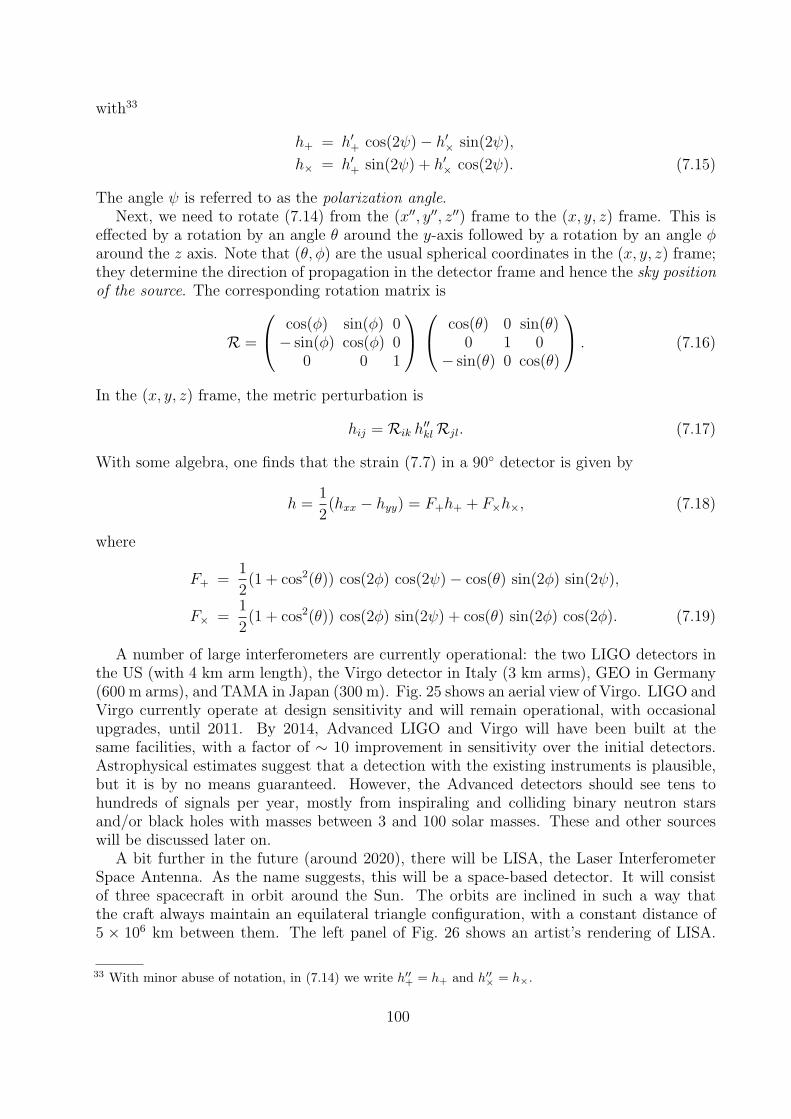
with33

h+ = h′+ cos(2ψ)− h′× sin(2ψ),

h× = h′+ sin(2ψ) + h′× cos(2ψ). (7.15)

The angle ψ is referred to as the polarization angle.Next, we need to rotate (7.14) from the (x′′, y′′, z′′) frame to the (x, y, z) frame. This is

effected by a rotation by an angle θ around the y-axis followed by a rotation by an angle φaround the z axis. Note that (θ, φ) are the usual spherical coordinates in the (x, y, z) frame;they determine the direction of propagation in the detector frame and hence the sky positionof the source. The corresponding rotation matrix is

R =

cos(φ) sin(φ) 0− sin(φ) cos(φ) 0

0 0 1

cos(θ) 0 sin(θ)0 1 0

− sin(θ) 0 cos(θ)

. (7.16)

In the (x, y, z) frame, the metric perturbation is

hij = Rik h′′klRjl. (7.17)

With some algebra, one finds that the strain (7.7) in a 90 detector is given by

h =1

2(hxx − hyy) = F+h+ + F×h×, (7.18)

where

F+ =1

2(1 + cos2(θ)) cos(2φ) cos(2ψ)− cos(θ) sin(2φ) sin(2ψ),

F× =1

2(1 + cos2(θ)) cos(2φ) sin(2ψ) + cos(θ) sin(2φ) cos(2φ). (7.19)

A number of large interferometers are currently operational: the two LIGO detectors inthe US (with 4 km arm length), the Virgo detector in Italy (3 km arms), GEO in Germany(600 m arms), and TAMA in Japan (300 m). Fig. 25 shows an aerial view of Virgo. LIGO andVirgo currently operate at design sensitivity and will remain operational, with occasionalupgrades, until 2011. By 2014, Advanced LIGO and Virgo will have been built at thesame facilities, with a factor of ∼ 10 improvement in sensitivity over the initial detectors.Astrophysical estimates suggest that a detection with the existing instruments is plausible,but it is by no means guaranteed. However, the Advanced detectors should see tens tohundreds of signals per year, mostly from inspiraling and colliding binary neutron starsand/or black holes with masses between 3 and 100 solar masses. These and other sourceswill be discussed later on.

A bit further in the future (around 2020), there will be LISA, the Laser InterferometerSpace Antenna. As the name suggests, this will be a space-based detector. It will consistof three spacecraft in orbit around the Sun. The orbits are inclined in such a way thatthe craft always maintain an equilateral triangle configuration, with a constant distance of5 × 106 km between them. The left panel of Fig. 26 shows an artist’s rendering of LISA.

33 With minor abuse of notation, in (7.14) we write h′′+ = h+ and h′′× = h×.

100

Figure 25: The French-Italian-Dutch Virgo detector is an interferometer with 3 km arm length.Together with the two LIGO detectors in the US it is poised to make a first gravitational wavedetection in the next several years.

As a rule of thumb, the larger the detector, the lower its frequency range; LISA will besensitive to gravitational waves with frequencies between 10−4 and 0.1 Hz. This in turnmeans that it will be picking up signals from sources with a much larger size. LISA willsee the inspiral and merger of binary supermassive black holes of a million to a billion solarmasses. Most galaxies are believed to have at least one such very massive black hole intheir centers (the one in our own galaxy contains some 4.1 million solar masses). Sometimesgalaxies merge together, in which case their central black holes will sink towards the middleof the newly formed, larger galaxy. They can then form a binary system and eventually theywill themselves merge to form a single black hole, emitting copious amounts of gravitationalradiation in the process.

Figure 26: Left: An artist’s impression of the Laser Interferometer Space Antenna, to be launchedaround 2020. Right: A possible lay-out for the Einstein Telescope.

Currently an EU-funded design study is in progress for a very advanced ground-basedfacility called ET, for Einstein Telescope. ET may consist of several interferometers, possiblyV-shaped and arranged in a triangle with 10 km sides. It is to be built some time after2020. ET will look for similar sources as Advanced LIGO and Virgo, but its sensitivity

101

will be another factor of 10 better. With a much larger number of sources as well asbetter measurement capabilities, it will be a prime instrument for studying the strong-fielddynamics of gravity.

B. Finding signals in noise

So far no gravitational wave detection has taken place, although as we shall see, a firstdetection will almost certainly happen within a decade from now. The data analysis problemis a formidable one: signals will be buried deep into the noise. A great variety of techniqueshave been developed to cope with this difficulty. In this chapter we will focus on a techniqueto search for signals of which the waveform is approximately known, but we emphasize fromthe outset that many other search methods are known and in use.

If an expected source can be modeled to the extent that its gravitational waveform ismore or less known, then one can apply matched filtering, and this is what we will discusshere.

So far we have pretended that detectors are noise-free and that the output, the strainh(t), is solely determined by the tidal action of gravitational waves on the interferometerarms. In reality, the measured strain, s(t), will be a superposition of the signal, h(t), andthe noise,34 n(t):

s(t) = n(t) + h(t). (7.20)

If the shape of the signal h(t) is more or less known, then one can integrate it against theoutput and divide by the observation time T :

1

T

∫ T

0

s(t)h(t) dt =1

T

∫ T

0

n(t)h(t) dt+1

T

∫ T

0

h(t)2dt. (7.21)

Both n(t) and h(t) are oscillating functions. However, the second integral in the RHS ispositive definite whereas the first one is itself oscillating. Heuristically,

1

T

∫ T

0

h(t)2dt ∼ h20, (7.22)

where h0 is the characteristic amplitude of the signal. On the other hand,

1

T

∫ T

0

n(t)h(t) dt ∼ τ0

Tn0h0, (7.23)

where n0 is the characteristic amplitude of the noise, and τ0 is the characteristic period.We see that in the limit T → ∞, the integral (7.23) will go to zero, but not (7.22). Inpractice, we can not make T arbitrarily large; indeed, the signals from coalescing binarieswill last for at most a few minutes, limiting T . Still, it is not necessary to have h0 > n0

in order to detect the signal; all that is needed is h0 > (τ0/T )1/2n0. Coalescing compact

34 There are many noise sources that contribute to n(t). The most important ones are thermal noise due tothe thermal vibrations of atoms in the optics of the interferometer, seismic noise, and shot noise due tothe fact that light has a particle as well as a wave character. All these phenomena degrade the accuracywith which an interferometer can measure relative length changes.

102

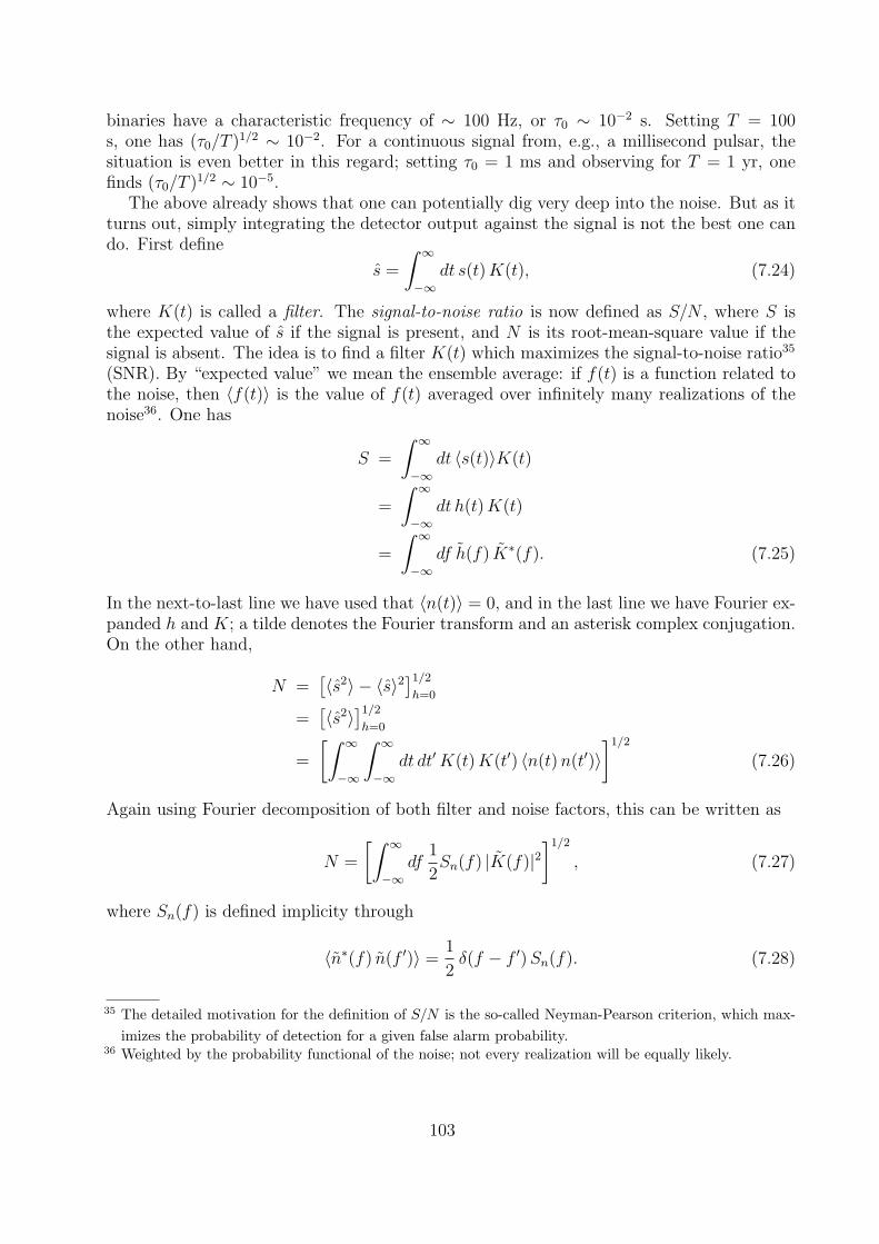
binaries have a characteristic frequency of ∼ 100 Hz, or τ0 ∼ 10−2 s. Setting T = 100s, one has (τ0/T )1/2 ∼ 10−2. For a continuous signal from, e.g., a millisecond pulsar, thesituation is even better in this regard; setting τ0 = 1 ms and observing for T = 1 yr, onefinds (τ0/T )1/2 ∼ 10−5.

The above already shows that one can potentially dig very deep into the noise. But as itturns out, simply integrating the detector output against the signal is not the best one cando. First define

s =

∫ ∞−∞

dt s(t)K(t), (7.24)

where K(t) is called a filter. The signal-to-noise ratio is now defined as S/N , where S isthe expected value of s if the signal is present, and N is its root-mean-square value if thesignal is absent. The idea is to find a filter K(t) which maximizes the signal-to-noise ratio35

(SNR). By “expected value” we mean the ensemble average: if f(t) is a function related tothe noise, then 〈f(t)〉 is the value of f(t) averaged over infinitely many realizations of thenoise36. One has

S =

∫ ∞−∞

dt 〈s(t)〉K(t)

=

∫ ∞−∞

dt h(t)K(t)

=

∫ ∞−∞

df h(f) K∗(f). (7.25)

In the next-to-last line we have used that 〈n(t)〉 = 0, and in the last line we have Fourier ex-panded h and K; a tilde denotes the Fourier transform and an asterisk complex conjugation.On the other hand,

N =[〈s2〉 − 〈s〉2

]1/2h=0

=[〈s2〉

]1/2h=0

=

[∫ ∞−∞

∫ ∞−∞

dt dt′K(t)K(t′) 〈n(t)n(t′)〉]1/2

(7.26)

Again using Fourier decomposition of both filter and noise factors, this can be written as

N =

[∫ ∞−∞

df1

2Sn(f) |K(f)|2

]1/2

, (7.27)

where Sn(f) is defined implicity through

〈n∗(f) n(f ′)〉 =1

2δ(f − f ′)Sn(f). (7.28)

35 The detailed motivation for the definition of S/N is the so-called Neyman-Pearson criterion, which max-imizes the probability of detection for a given false alarm probability.

36 Weighted by the probability functional of the noise; not every realization will be equally likely.

103

Sn(f) is called the noise spectral density, with units of Hz−1. It describes in which way thenoise is correlated with itself.37 Integrating over frequency, it also yields the variance of thenoise in the time domain: ∫ ∞

0

df Sn(f) = 〈n2(t)〉 = 〈n2(t = 0)〉, (7.29)

where we have used that Sn(−f) = Sn(f), as follows from its definition (7.28).Putting everything together, we find that the signal-to-noise ratio is

S

N=

∫∞−∞ df h(f) K∗(f)[∫∞

−∞ df12Sn(f) |K(f)|2

]1/2. (7.30)

We still need to find the filter K(t) which maximizes S/N . This can most easily be donealgebraically, by introducing the following inner product:

(a|b) ≡ Re

∫ ∞−∞

dfa∗(f) b(f)

12Sn(f)

= 4 Re

∫ ∞0

a∗(f) b(f)

Sn(f). (7.31)

With this definition, one can write S/N as

S

N=

(K|h)

(K|K)1/2, (7.32)

where

K =1

2Sn(f) K(f). (7.33)

With the definition (7.31), the SNR is just the inner product of the signal waveform withthe unit vector (7.33). Clearly, to maximize the SNR we need to choose K(t) in such a way

that this unit vector points in the same direction as h(f). This is effected by choosing thefilter’s Fourier transform to be

K(f) ∝ h(f)

Sn(f), (7.34)

which is the so-called Wiener filter. The proportionality constant is unimportant, as thevector K only affects the SNR in normalized form. With (7.34), the optimal SNR becomes

S

N= (h|h)1/2

= 4

∫ ∞0

|h(f)|2

Sn(f). (7.35)

This result makes intuitive sense. The optimal filter should not just depend on the signal’swaveform, but also on the properties of the noise. In particular, at frequencies where there is

37 Note that Eq. (7.28) is not only the definition of Sn(f). It also implies an assumption on the noise, namelythat it is stationary, i.e., its different Fourier components are uncorrelated.

104

more noise (larger Sn(f)), the filter should get suppressed; where there is less noise (smallerSn(f)), it should have more weight.

We will have more to say about signal-to-noise ratios later, when discussing individualsources. For now we stress that in practice, the optimum (7.35) is never reached. Formany sources we know the waveform family, but the signal could be any waveform fromthis continuous set.38 This is the case with the inspiral and coalescence of compact binaryobjects such as neutron stars and black holes. These come in a wide variety of masses,and different masses lead to different waveforms. To cover the presumed parameter space,one must search the data with a wide variety of filters h(f ; θ)/Sn(f), each with differentvalues for the parameters θ = θ1, . . . , θN characterizing the waveforms.39 Of necessity, thenumber of filters will be finite, and the relevant part of parameter space will only be probedby a sprinkling of points in it. Such a discrete collection of filters h(f ; θ)/Sn(f) is called atemplate bank. Next, the noise is not really stationary, as was assumed in the very definitionof the spectral density; see Eq. (7.28) and the associated footnote. To take this into account,in practice a new template bank is generated on a regular basis; in the search for binarycoalescences with LIGO and Virgo a new bank is made for every 2048 s of data. “Glitches”in the data are often sufficiently similar to a signal from a known waveform family that itgenerates an SNR above the pre-set threshold; in a typical week there will be thousands ofsuch events. A detection will not be declared unless a candidate signal is seen more or lesssimultaneous in at least two different detectors, and if the templates that give the highestSNRs in individual detectors are associated with similar parameter values.

In practice, the data analyst does not quite define SNR as we did above. In the definitionof S, Eq. (7.25), he/she has no access to an “expected” value of 〈s(t)〉, only to the datastream that actually came out of the detector, s(t). Regarding N , one can take Eq. (7.27)at face value, and construct a noise spectral density Sn(f) from Eq. (7.28) by pretendingthat the noise is stationary and only considering correlation between noise Fourier modes ofthe same frequency. Given these considerations and going through similar steps as above,one arrives at

S

N= max

θ

(h(θ)|s)√(h(θ)|h(θ))

. (7.36)

This brings us to the issue of parameter estimation. Having to ability to infer, say,the component masses in candidate coalescence signals with good accuracy is important inreducing false alarm rates when comparing near-simultaneous triggers in different detectors.Moreover, when a detection is actually made, we will want to extract as much physicalinformation about the source as we possibly can.

Although the above caveats should be kept in mind, we will continue to make somewhatidealized assumptions about the data. In particular, we will take it to be not only stationarybut also Gaussian; i.e., we assume that the probability distribution for different realizationsof the noise takes the form

P (n) = N exp

[−1

2

∫ ∞−∞

df|n(f)|212Sn(f)

], (7.37)

38 There will also be inaccuracies in the modeling of the waveforms; obtaining more faithful waveform familiesis currently an object of intense research

39 In the case of some parameters it may be possible to maximize the SNR over them analytically, but usuallynot for all.

105

where the variance of the Fourier mode with frequency f was taken to be proportional to(1/2)Sn(f), following Eq. (7.28). Using the inner product (7.31), this can be written moresuccinctly as

P (n) = N exp [−(n|n)/2] . (7.38)

Now imagine that the conditions for claiming a detection are satisfied. Then the detectoroutput is of the form s(t) = n(t) + h(t; θ), with n(t) a realization of the noise and h(t; θ)the signal, with parameter values θ = θ1, θ2, . . . , θN. The latter are a priori unknown, astemplate waveforms that cause the largest SNR may have different parameter values fromthe signal. Using the distribution (7.37), we can write down the likelihood that a particulardetector output s(t) is seen given that there is a signal with parameters θ in the data:

P (s|θ) = N exp [−(s− h(θ)|s− h(θ))/2] . (7.39)

Now we used Bayes’s theorem, which says that for statements A and B, the probability thatA is true given B can be written as

P (A|B) =P (B|A)P (A)

P (B), (7.40)

where P (B|A) is the probability of B if A is given, and P (A), P (B) are the overall prob-abilities for A and B, respectively. Applied to our problem, A could be a set of parametervalues θ, and B a realization of the detector output s(t). Hence,

P (θ|s) =P (s|θ)P (θ)

P (s). (7.41)

Since in the above, s is a given, we will be able to absorb the denominator P (s) in the RHSinto an overall prefactor. In the Bayesian approach to statistics, which we are adoptinghere, the prior probability P (θ) quantifies any prior knowledge as well as assumptions. Forinstance, neutron star masses are known to be sharply peaked around 1.35M; regardingdistances, for isotropic sources one can assume a prior distribution p(0)(r) dr ∝ r dr forsources in the galactic disk, or p(0)(r) dr ∝ r2dr for extragalactic sources. If one does notwant to include any prior assumptions, one adopts a uniform prior p(0) = const, which canthen be absorbed into the normalization factor N . This is what we will do here. Puttingeverything together, we get

P (θ|s) = N exp

[(h(θ)|s)− 1

2(h(θ)|h(θ))

], (7.42)

where we also absorbed a factor exp [−(s|s)/2] into the overall prefactor N (again, s is agiven).

To arrive at error estimates, it is convenient to find the peak of the distribu-tion P (θ|s). In the case of a flat prior, the location of the peak θML is called themaximum likelihood estimator. If p(0) is constant, then maximizing P (θ|s) is the same as

maximizing P (s|θ), which is given by (7.39). This gives θML an elegant geometric interpret-ation. The family of signal waveforms h(t; θ) can be viewed as a manifold. The additionof noise n(t) takes us out of this manifold, giving an output s(t). Now, Eq. (7.39) tellsus that maximizing P (s|θ) is the same as minimizing (s − h(θ)|s − h(θ)). The quantity(s − h(θ)|s − h(θ)) has a natural interpretation as the square of the distance between the

106

detector output s and the waveform h(θ) in the manifold of signals. Hence, the maximum

likelihood estimator θML is the set of values θ that gives the minimal distance squaredbetween the detector output and the signal manifold.

The maximum likelihood estimator has another interesting property, which is that it alsogives the parameter values which maximize the SNR, Eq. (7.36). To see this, let us returnto Eq. (7.42). Maximizing P (θ|s) is the same as maximizing its logarithm,

logP (θ|s) = (h(θ)|s)− 1

2(h(θ)|h(θ)) + const. (7.43)

Now write h(t; θ) = Ah0(t; θ′), where A is an amplitude, and we have made the split θ =A, θ′ (i.e., θ′ denotes all remaining parameters). One then has40

logP (θ|s) = A(h0(θ′)|s)− A2

2(h0(θ′)|h0(θ′)). (7.44)

Setting ∂ logP (θ|s)/∂A = 0, we find the maximum likelihood estimate for A,

AML =(h0(θ′)|s)

(h0(θ′)|h0(θ′)). (7.45)

Substituting this back into (7.44), we get

maxA

logP (θ|s) =1

2

(h0(θ′)|s)2

(h0(θ′)|h0(θ′)). (7.46)

Multiplying by A2 in numerator and denominator and maximizing over the remaining para-meters, we find

maxθ

logP (θ|s) =1

2maxθ

(h(θ)|s)2

(h(θ)|h(θ)). (7.47)

Since the maximum likelihood values θML are, by definition, the θ values that maximize theLHS, the above tells us that θML are also the values that maximize the SNR as given byEq. (7.36).

If the SNR is large, then parameter uncertainties will be small. In the expression (7.42),

one can then expand the exponent around θML, writing θ = θML + δθ and only retainingleading-order terms in δθ. Recall that θ is actually a set of paramaters θi, i = 1, . . . , N , sosimilarly we have a set of δθi. Now, to first order,

h(t; θ) = h(t; θML) + ∂ih(t; θML) δθi, (7.48)

where ∂i = ∂/∂θi. In the exponent of (7.42), all zeroth order terms can be absorbed into

N . Any terms linear in the δθi will vanish since by definition, θML minimizes the exponent.Hence the leading order non-trivial contributions to the exponent are the quadratic ones,and in that approximation P (θ|s) takes the form

P (δθ) = N exp

[−1

2Γijδθ

iδθj], (7.49)

40 In what follows we ignore the constant contribution in the previous equation, as it is irrelevant for therest of the discussion

107

whereΓij = (∂i∂jh|h− s) + (∂ih|∂jh). (7.50)

In the first term, h − s = −n, and in the limit of large signal-to-noise ratio, |h| dominatesover |n|. Hence, in this limit,

Γij = (∂ih|∂jh). (7.51)

This is called the Fisher information matrix. One can show the following:

〈δθiδθj〉 = (Γ−1)ij, (7.52)

where in this case 〈. . .〉 denotes the average with respect to the probability density P (δθ) asin (7.49), with Γij as in (7.51). For a function f(δθ),

〈f(δθ)〉 =

∫d(δθ1)

∫d(δθ2) . . .

∫d(δθN)f(δθ)P (δθ). (7.53)

The matrixΣij ≡ (Γ−1)ij (7.54)

is called the covariance matrix. From Eq. (7.52)

∆θi ≡√〈(δθi)2〉 =

√Σii, (7.55)

where in the last equality there is no summation over repeated indices. Thus, the squareroots of the diagonal elements of Σ allow us to estimate the root-mean-square (i.e., 1-σ) un-certainties on the parameters. The other elements give the covariances between parameters,as Eq. (7.52) also shows:

〈δθiδθj〉 = Σij. (7.56)

These are often normalized to give numbers between -1 and 1, called the correlation coeffi-cients :

cij ≡ Σij

√ΣiiΣjj

. (7.57)

If the correlation between two parameters is close to zero, then they are essentially independ-ent from each other as far as the measurement problem is concerned. If cij ' −1 (stronglyanti-correlated) or cij ' +1 (strongly correlated) then it will be hard to disentangle θi and θj

from the information contained in the signal. In that case it will be difficult to measure themseparately, although a combination of them may still be measurable with good accuracy.

We stress once again that the covariance matrix formalism as outlined above relies onthe SNR being large, which often will not be the case. Nevertheless, the formalism iswidely used to give an indication of the accuracy with which quantities can be measuredusing gravitational wave observations. An important application has been in the analysisof signals from inspiraling compact binaries. If more less simultaneous triggers are seen intwo detectors, then one can use the formalism to estimate the uncertainty in the parametersin the individual detectors, assuming a real signal is involved. The parameters associatedwith the templates that gave the largest SNR give the values of θML in each of the detectors,and the covariance matrices give the 1-σ uncertainty intervals around these values (whichfor safety’s sake are then multiplied by some factor). One then compares these intervals inthe two detectors for all of the parameters involved. If none of them overlap, then the eventcan confidently be dismissed as having been spurious and not a gravitational wave signal.When a first gravitational wave signal is seen, the covariance formalism will give us a roughidea of what kind of source we are dealing with, after which more sophisticated techniqueswill be used for further investigations.

108

VIII. ASTROPHYSICAL SOURCES OF GRAVITATIONAL RADIATION

A. Inspiral of compact binaries

We have seen how gravitational waves are generated, what their action is on test particles,and what energy they carry. Let us now turn to applications, the first one being the inspiralof compact binaries.

First consider two compact objects (neutron stars and/or black holes) being in a circularorbit around their center of gravity with a sufficiently large separation R between the bodies,so that the energy carried away by gravitational radiation is very small and the orbits canbe considered fixed over at least one period. In addition let’s assume that R Rschw1,2

where the latter are the objects’ Schwarzschild radii, set by their masses m1 and m2; inthat case they can also be considered as point particles. They move on a circle with radius(µ/mi)R, i = 1, 2, with µ = m1m2/(m1 + m2) the reduced mass; setting the associatedcentripetal force equal to the Newtonian gravitational force acting over the separation R,one finds Kepler’s law:

ω2orb =

GM

R3, (8.1)

where ωorb is the angular orbital frequency.To leading order in velocity, gravitational radiation results from the time evolution of the

quadrupole moment and is described by Eq. (6.122). An brief calculation shows that thequadrupole gravitational wave polarizations are given by

h+(t) =4

r

(GMc

c2

)5/3(πfgw

c

)2/31 + cos2(ι)

2cos(2πfgwtret + 2φ),

h×(t) =4

r

(GMc

c2

)5/3(πfgw

c

)2/3

cos(ι) sin(2πfgwtret + 2φ). (8.2)

Note how the component masses m1, m2 only enter the amplitude through a particularcombination called the chirp mass :

Mc =(m1m2)3/5

(m1 +m2)1/5(8.3)

The reason for the name will become later on. The frequency of the emission, fgw is doublethe orbital frequency,

fgw = 2forb = 2ωorb

2π. (8.4)

This is because for a rigidly rotating system, in the center of mass frame the componentsof the quadrupole tensor return to the same value after only half a period. fgw is normallycalled the gravitational wave frequency. This is apt if only quadrupole radiation is beingstudied, but in reality also higher multipole moments will come into play. These introduceharmonics with frequencies nforb, n = 1, 2, 3, . . .. However, the harmonic with n = 2 isthe dominant contribution to the gravitational waveform, all others being sub-leading by atleast one power of v/c.

The waveforms (8.2) can be written in an instructive form by associating a length scalewith both the chirp mass and the gravitational wave frequency. With the chirp mass we can

109

associate a characteristic radius,

Rc =2GMc

c2, (8.5)

which would be the radius of a spherical black hole with mass Mc. The gravitational wavefrequency can be converted into a wavelength,

λ =c

fgw

. (8.6)

The gravitational wave polarizations (8.2) then become

h+ = A1 + cos2(ι)

2cos(2πfgwtret + 2φ),

h× = A cos(ι) sin(2πfgwtret + 2φ), (8.7)

with

A =

(2π√

2

)2/3(Rc

r

) (Rc

λ

)2/3

. (8.8)

The more mass involved, the larger Rc and the larger the amplitude. The wavelength ofthe gravitational radiation, λ, gives a sense of the size of the binary itself: the tighter thebetter. Also note that the radiation is not isotropic: more gets emitted perpendicularly tothe orbital plane. If ι = 0 then the overall amplitudes of the two polarizations in (8.7) areequal, and there is only a π/2 phase difference between the two. On the other hand, insidethe orbital plane (ι = π/2), the amplitude of h+ is only half as big, and h× is identicallyzero. Perpendicular to the plane, the radiation is an equal admixture of the “plus” and“cross” polarization; this is called circular polarization. By contrast, an observer watchingthe binary in the orbital plane only sees the components move back and forth on a linesegment, and only one of the two polarizations is present, aligned with that segment: linearpolarization. For 0 < ι < π/2 one has elliptical polarization.

One can also look at the way power is emitted in different directions. From Eq. (6.86),we see that the power41 emitted per unit solid angle is

dPgw

dΩ=

r2c3

16πG〈h2

+ + h2×〉 (8.9)

Inserting our expressions (8.2) for compact binaries, and keeping in mind that 〈cos2(ωt +ϕ)〉 = 〈sin2(ωt+ ϕ)〉 = 1/2, this becomes

dPgw

dΩ=

2

π

c5

G

(GMcπfgw

c3

)10/3

g(ι), (8.10)

where

g(ι) =

(1 + cos2(ι)

2

)2

+ cos2(ι). (8.11)

41 Not to be confused with the momentum P i.

110

Hence eight times as much power is emitted perpendicular to the orbital plane than into theplane. Integrating over the sphere we find the total radiated power:

Pgw =

∫dΩ

dPgw

dΩ

=32

5

c5

G

(GMcπfgw

c3

)10/3

. (8.12)

So far we have been assuming that the components of the binary are on fixed orbits. Fornon-relativistic systems, the total orbital energy is

Eorb = Ekin + Epot

= −Gm1m2

2R. (8.13)

Since gravitational waves carry away energy, Eorb should become more and more negative,which can only happen if R decreases. In fact, from (8.1),

R = −2

3Rωorb

ωorb

(8.14)

= −2

3(Rωorb)

ωorb

ω2orb

. (8.15)

Note that R is the radial velocity while Rωorb is the tangential velocity. The above tells usthat if

ωorb ω2orb, (8.16)

then the radial motion is very small compared to the tangential motion; when this conditionholds, the motion is said to be quasi-circular, and the binary is in the inspiral regime. Inwhat follows we will assume to be in this regime.

Using (8.1), and keeping in mind (8.4), one can eliminate R in the expression for theorbital energy in favor of the gravitational wave frequency fgw:

Eorb = −(G2M5

cπ2f 2

gw

8

)1/3

. (8.17)

The loss in orbital energy per unit of time can be equated to the total energy flux of thegravitational wave emission:

−dEorb

dt= Pgw. (8.18)

Using (8.17) and (8.12), this gives an expression for the time evolution of the frequency:

fgw =96

5π8/3

(GMc

c3

)5/3

f 11/3gw . (8.19)

This can be integrated to obtain fgw as a function of time:

fgw(τ) =1

π

(GMc

c3

)−5/8(5

256

1

τ

), (8.20)

111

with τ = tcoal − t, where the coalescence time tcoal is the time at which fgw(τ) formallydiverges. Note, however, that apart from the emission of gravitational radiation, we aretreating the orbital motion in a Newtonian way. In a fully relativistic treatment, therewould be an innermost stable circular orbit (ISCO). In the case where m1 m2 (so thatwe may view m2 as a test mass in a Schwarzschild geometry with mass m2 'M , the radiusof such an orbit is

risco =6GM

c2. (8.21)

Within the Schwarzschild spacetime, massive test particles can not be on circular orbits witha radius smaller than risco. Using (8.1) and (8.4), the gravitational wave frequency at ISCOis

fgw,isco =c3

63/2πGM. (8.22)

If m1 and m2 are comparable, then one point mass can no longer be considered a test particlein the Schwarzschild geometry of the other, but there will still be an ISCO frequency beyondwhich the waveforms (8.2) are no longer valid. As it turns out, also in the general case it issafe to use the expression (8.22) as a rule of thumb for the breakdown of the quasi-circularregime. After that, the particles will plunge towards each other and collide.

As the frequency increases, the separation between the point masses shrinks. From (8.14)and (8.20),

R

R= −2

3

fgw

fgw

= − 1

4τ, (8.23)

where we recall that τ = tcoal − t. Integrating this, we obtain

R(τ) = R0

(τ

τ0

)1/4

= R0

(tcoal − ttcoal − t0

), (8.24)

with R0 the value of R at some initial time t0, and τ0 = tcoal − t0.Note that in the derivation of (8.2), fgw and R were considered constant. If the orbit

evolves then the motion will be described by

x1(t) =µ

m1

R(t) e(t),

x2(t) = − µ

m1

R(t) e(t), (8.25)

where R(t) is as in (8.24), and

e(t) = (cos(Φ(t)/2), cos(ι) sin(Φ(t)/2), sin(ι) sin(Φ(t)/2)). (8.26)

and R(t) is as in (8.24). We have defined

Φ(t) = 2

∫ t

dt′ ωorb(t′)

=

∫ t

dt′ ωgw(t′), (8.27)

112

with ωgw(t) = 2πfgw(t). When using the quadrupole expressions (6.122) to compute h+, h×,in the arguments of the trigonometric functions we must now replace ωgwt by Φ(t). When

computing M11, M22, and M12, time derivatives of R(t) and ωgw(t) will now also appear.

However, in the quasi-circular approximation, R(t) can be neglected. The orbital (and hencegravitational wave) frequency will then also not change significantly over a single orbit, andwe can also neglect ωgw. This means that in the expressions (8.2), in the arguments of thecosine and sine we may replace 2πfgwt by Φ(t), and in the amplitudes the constant fgw canbe replaced by fgw(t), with time dependence as in (8.20). All these are to be evaluated atthe retarded time tret. The inspiral gravitational waveforms are then

h+(t) =4

r

(GMc

c2

)5/3(πfgw(tret)

c

)2/31 + cos2(ι)

2cos(Φ(tret)),

h×(t) =4

r

(GMc

c2

)5/3(πfgw(tret)

c

)2/3

cos(ι) sin(Φ(tret)). (8.28)

Using (8.20) in (8.27), one has

Φ(t) = −2

(5GMc

c3

)−5/8

τ 5/8(t) + Φc, (8.29)

where the integration constant Φc is the phase at coalescence, and we recall that τ = tcoal−t.Let us take stock. Gravitational wave emission causes a binary system to lose orbital

energy, leading the orbits to shrink. We have derived the gravitational waveforms in thequadrupole approximation, and under the assumption that the system can be assumedto behave in a Newtonian way, consistent with the assumption of small v/c underlyingthe quadrupole treatment. In the quasi-circular inspiral regime, where ωgw ω2

gw, boththe waveform amplitudes and the frequency increase monotonically – the binary “chirps”.How fast the amplitudes and frequency evolve is determined by a particular combination ofthe component masses, the chirp mass Mc. Eventually our description must break down,because of the concept of innermost stable circular orbit (ISCO) in general relativity. Thecomponents of the binary then plunge towards each other and merge.

What kind of objects might be suitable for observation of their gravitational wave signalwith existing detectors? The large ground-based interferometric detectors have a frequencyrange between approximately 20 Hz and 1 kHz, with a strain sensitivity h ∼ 10−22. Fromthe exercises above we already know that Earth-based experiments involving masses beingrotated at technologically feasible speeds will not generate detectable gravitational waves.The motion of planets in our solar system also doesn’t generate sufficiently strong gravit-ational radiation, and in any case the frequency is far too low; for the Earth-Sun system,fgw = 2/(365 × 24 × 3600 s) ' 6.4 × 10−8 Hz. Earth-based experiments involving massesbeing rotated at technologically feasible speeds will also not generate detectable gravita-tional waves. Hence we need to look for sources in space. Most stars are in fact membersof a binary system, so can we detect their gravitational radiation signature? Let’s considera binary consisting of two ordinary stars with m1 = m2 = 1M. When the signal fromsuch a binary enters the band, i.e., when fgw = 20 Hz, Kepler’s law (8.1) tells us that theseparation is only about 400 km. Ordinary stars have radii in the order of 106 km. In otherwords, already when their gravitational wave frequency would enter the detector band, nor-mal stars would already have merged completely and could no longer be considered separate

113

objects! Clearly the stars would need to be far more compact. Consider white dwarfs, theembers of normal stars that have spent their nuclear fuel and are kept from collapsing onlyby electron degeneracy. The maximum mass of a white dwarf is 1.4 M (the Chandrasekharlimit), and a white dwarf binary at fgw = 20 Hz would have a separation of just over 450km. But a typical white dwarf radius is about 104 km, which doesn’t solve the problem42.

Even more compact are neutron stars. These are the result of a very massive star havingundergone supernova. If the density of the remnant object in the center is large enough thatelectron degeneracy is overcome, electrons and protons are forced to combine into neutrons.Neutron stars also have a typical mass of 1.4M but a radius of only 10 km. Binary neutronstars would still be sufficiently well-separated when their gravitational wave signal enters theband of a ground-based detector. At the innermost stable circular orbit, one has fgw = 1566Hz, corresponding to a separation of 40 km. Hence even then they will still be separateobjects, and one can show that the point particle approximation is still an acceptable one.

Finally there are black holes, with typical masses of ∼ 5M. Two such black holes in abinary would then have M = 10M, corresponding to a separation of about 700 km whenfgw = 20 Hz. Each has a Schwarzschild radius of Gmi/c

2 ' 7.4 km, i = 1, 2. At ISCO,fgw,isco = 438 Hz, implying a separation of 140 km.

Clearly, at least in terms of frequency and size, binary neutron stars and black holes (andalso mixed systems consisting of a neutron star and a black hole) are potential sources forground-based detectors. Although several binary neutron stars have been discovered in ourgalaxy, they are hundreds of millions of years away from merger. Neutron star or black holebinaries that are tight enough that merger is imminent (i.e., that fgw & 20 Hz are thoughtto be exceedingly rare.

The expression (8.20) for fgw as a function of time can be inverted; in terms of observa-tionally interesting quantities,

τ = 2.18 s

(1.21MMc

)5/3(100 Hz

fgw

)8/3

. (8.30)

Here 1.21M is the chirp mass of a binary with m1 = m2 = 1.4M (two neutron stars). Atfgw = 20 Hz, this gives τ = 160 s while at fgw,isco = 1566 Hz, τ = 0.0014 s; hence the inspiralsignal will be in band for just under 3 minutes. In the case of a (5, 5)M binary black hole,Mc = 4.32M, and the signal will remain in band for 19 s. The most massive systems aground-based detector can see with the given lower cut-off frequency have fgw,isco ' 20 Hz;for an equal-mass binary this corresponds to M ' 200M.

Another interesting quantity is the number of waveform cycles within the detector’s band:

Ncyc =

∫ tmax

tmin

fgwdt

=

∫ fmax

fmin

fgw

fgw

dfgw. (8.31)

42 However, binary white dwarves will be sources for the space-based detector LISA. In that case the sens-itivity band starts at 10−4 Hz, and the corresponding separation is about 1.5 × 106 km, which is largeenough. In fact, LISA will pick up so many signals from binary white dwarves in our galaxy that theywill cause “confusion noise”.

114

Expressing fgw in terms of fgw itself using Eq. (8.19) and integrating we get

Ncyc =1

32π8/3

(GMc

c3

)−5/3

(f−5/3min − f−5/3

max )

' 5× 103

(20 Hz

fmin

)5/3(1.2Mc

M

)5/3

. (8.32)

Thus, a signal will have hundreds to thousands of cycles in band. This makes it imperativeto have a good understanding of the waveform, and especially its phasing, so that theparameters characterizing the sources can extracted with great accuracy. The expression(8.29) is merely the leading-order contribution in an appropriate expansion parameter, e.g.,Θ ≡ (5GMc/(c

3τ))1/8. Such an expansion is currently known to 7th order in Θ.Next we turn to detection and parameter estimation. Given an interferometer with beam

pattern functions F+ and F×, and the signal’s polarizations h+ and h×, the measured strainwill be

h(t) = F+(θ, φ, ψ)h+(t) + F×(θ, φ, ψ)h×(t). (8.33)

The sky position (θ, φ) enters the strain through the beam pattern functions; the same goesfor the polarization angle ψ, which gives the orientation of the long axis of the orbit as seenon the sky. The other parameters in the problem enter through the polarizations; these are

m1,m2, ι, tc,Φc, r. (8.34)

Here (m1,m2) are the component masses; ι gives the inclination of the orbital plane withrespect to the line of sight; tc is the time of coalescence, Φc the phase at coalescence, and rthe distance. It is convenient to rewrite (8.33) as

h(t) =√F 2

+(1 + cos2(ι)) + F 2×4 cos2(ι) cos(Φ(t) + ϕ0), (8.35)

with

ϕ0 = arctan

(− F×2 cos(ι))

F+(1 + cos2(ι))

). (8.36)

The calculation of the signal-to-noise ratio, Eq. (7.35), and the Fisher matrix, Eq. (7.51)both require the strain in the Fourier domain. The strain is time-dependent through the timedependence of the polarizations h+(t) and h×(t); hence we will need the Fourier transforms ofthese. Although one can use numerical methods, such as the Fast Fourier Transform (FFT),it is instructive to have some analytical insight. An analytic expression can be obtainedthrough the stationary phase approximation, which is valid if for a waveform’s amplitudeA(t) and phase φ(t), one has |(1/A)dA/dt| 1 and |d2φ/dt2| (dφ/dt)2. We will not gointo details here but will just state that the Fourier transform of the strain in the stationaryphase approximation is given by

h(f) = −√F 2

+(1 + cos2(ι))2 + F 2×4 cos2(ι)

√5π

96(πf)−7/6 c

r

(GMc

c3

)5/6

× exp[i(

2πftc + Ξ(f)− ϕ0 −π

4

)], (8.37)

where, at leading order,

Ξ(f) = −Φc +3

8

(8πGMcf

c3

). (8.38)

115

In this approximation, the optimal SNR (7.35), which we will denote by ρ, is given by

ρ =

[(F 2

+(1 + cos2(ι))2 + F 2×4 cos2(ι)

) 5π

24π−7/3 c

2

r2M5/3

c

∫ fmax

fmin

f−7/3

Sn(f)

]1/2

, (8.39)

where [fmin, fmax] is the detector’s sensitivity band and Sn(f) its power spectral density.From the above expression as well as the beam pattern functions (7.19) for an L-shapedinterferometer, one sees that for given component masses and distance, the SNR is largestwhen ι = 0, i.e., when the system is seen face-on, and either θ = 0 or θ = π, i.e., when thedirection to the binary is perpendicular to the detector plane. In that case

ρopt =

[5π

6π−7/3 c

2

r2M5/3

c

∫ fmax

fmin

f−7/3

Sn(f)

]1/2

. (8.40)

One can also take the average over both sky position and orientation of the binary. A briefcalculation shows that ⟨

F 2+

(1 + cos2(ι)

2

)2

+ F 2× cos2(ι)

⟩=

4

25, (8.41)

hence the SNR averaged over all angles is

ρave =2

5ρopt. (8.42)

Demanding some minimum SNR, one can now ask to what distance a binary with givenmasses can be seen. A good indicator is the angle-averaged horizon distance, obtained bysolving for r in the expression for the angle-averaged SNR. This leads to

dhor =2

5

[5π

6π−7/3c2M5/3

c

∫ fmax

fmin

f−7/3

Sn(f)

]1/2

ρ−10 . (8.43)

The left panel of Fig. 27 shows dhor for initial LIGO and Virgo at design sensitivity, and forAdvanced LIGO, as a function of total mass for equal mass binaries, for a minimum SNR of5. Binary neutron stars with Mtot = 2.8M can seen in initial detectors out to ∼ 20 Mpc,and to ∼ 300 Mpc in Advanced LIGO. For binary black holes with Mtot = 10M, initialdetectors are sensitive up to ∼ 50 Mpc while Advanced LIGO can seen them out to abouta Gpc. One might think that the detection rate will scale roughly with the cube of horizondistance, but this is not the case. Fig. 28 illustrates the reason why: binary coalescenceevents tend to take place in galaxies, which are not at all uniformly distributed over volume.In our immediate intergalactic vicinity, the richest clusters are the Virgo Cluster (∼ 20 Mpc)and the Coma Cluster (∼ 100 Mpc).

Astrophysicists try to model how frequently close binary systems composed of neutronstars and/or black holes form; combined with the projected horizon distances as in Fig. 27,this gives predictions for detection rates. Table I gives the likely range of detection rates forthe initial (currently operational) LIGO/Virgo network, and for the network of Advanceddetectors. The uncertainties are very large due to the difficulties in astrophysical modeling,but in the era of advanced detectors (around 2015), regular detections are to be expec-ted. Much effort is currently being put into the construction of the instrumentation, andpreparations for extracting science from the first detections.

116

Figure 27: Angle-averaged horizon distances for initial Virgo (green dashed line), initial LIGO (reddash-dotted line) and Advanced LIGO (solid black line), as a function of total mass, for binarieswith equal component masses. The assumed SNR threshold is ρ0 = 5.

Network Source Nlow Nre Nhigh

(yr−1) (yr−1) (yr−1)NS-NS 2× 10−4 0.02 0.2

Initial NS-BH 7× 10−5 0.0004 0.1BH-BH 2× 10−4 0.007 0.5NS-NS 0.4 40 400

Advanced NS-BH 0.2 10 300BH-BH 0.4 20 1000

Table I: Detection rates for the initial (i.e., currently operational) network of ground-based de-tectors, and for the advanced detectors which will become operational in 2015. There are hugeuncertainties due to the difficulties in modeling the formation of binary systems; here we show res-ults from models with low predicted rates, realistic rates, and high rates. The sources are binaryneutron stars (NS-NS), binaries consisting of a neutron star and a black hole (NS-BH), and binaryblack holes (BH-BH). Regular detections are extremely likely once the advanced detectors becomeavailable.

The above considerations are for ground-based detectors only. Around 2020, the space-based LISA will be launched. Being a far larger instrument (with the three probes at 5million km from each other), LISA will be sensitive to gravitational waves with much largerwavelengths, and hence much lower frequencies: between 10−4 Hz and 0.1 Hz. The sourcesLISA will have access to will be supermassive black holes such as the ones that lurk inthe centers of galaxies. When two galaxies merge, the supermassive black holes will tendto sink to the center of the new galaxy that is formed, and they might then form a binarysystem. Such systems are already being observed with conventional telescopes; Fig. 29 showsa binary supermassive black hole in the galaxy NGC 6240. To see why LISA is sensitive tothese kinds of systems, one can write the expression for the gravitational wave frequency at

117

Figure 28: The distance reach of initial versus Advanced LIGO for binary neutron stars. The whitedots are galaxies; note the strong clustering.

ISCO as

fgw,isco =c3

63/2πGM' 1.75× 10−2 106M

MHz. (8.44)

Given the sensitivity range f ∈ [10−4, 0.1] Hz, we see that systems will be visible for totalmasses roughly between 105M and 108M. They will also be in the frequency band for avery long time. Consider a system with M = 106M so that fgw,isco is 1.75×10−2 Hz. Usingthe expression (8.30) for the time to coalescence as a function of frequency, at fgw = 10−4

Hz one has τ = 1.2× 107 s, while at fgw,isco, τ = 12.5 s. Hence the signal is in band for fourand a half months!

Depending on their component masses, sky position, and orientation, supermassive bin-aries up to redshifts of z = 1 can give signal-to-noise ratios in the thousands, and LISA willbe able to see inspirals up to z > 15, when black holes were in the process of being formed

118

Figure 29: A picture of what is almost certainly a binary supermassive black hole in the center ofthe galaxy NGC 6240, made with the Chandra X-ray satellite. The luminous spots are accretiondisks around the black holes. This particular system is still very far from merger, but other, muchtighter supermassive binaries are primary sources for LISA.

for the first time. In other words, LISA will see all eligible sources in its past light cone!Although the expected detection rate is again dependent on astrophysical modeling, theiris broad agreement that there should be between 20 and 80 detections per year, and LISAmay be operational for several years.

Due to the large signal-to-noise ratios, LISA will be a prime instrument for studying thedynamics of gravity in the strong field regime and to look for possible deviations from GR.Such information can be gleaned not only from the inspiral signal, but also from the mergersignal itself, and the “ringing” of the single black hole that results from it.

Other interesting sources for LISA are Extreme Mass Ratio Inspirals (EMRIs), where asmaller black hole spirals into a very massive one, possibly on very excentric orbits exhibitinghuge perihelion precession. By studying the gravitational wave signal, the orbits can betraced in great detail, which in turn will provide in-depth information about the geometry ofspacetime in the immediate vicinity of the more massive black hole; this is what is illustratedin Fig. 30. This will provide accurate tests of the Black Hole Uniqueness Theorem, whichstates that black hole geometries are only determined by43 the mass M and the rotationalangular momentum J .

B. Gravitational waves from spinning neutron stars

Another interesting source of gravitational radiation is a spinning, isolated neutron star44.Neutron stars are axisymmetric to a high degree; in particular they are oblate due to their

43 Technically also by the electric charge Q, but astrophysical black holes will be electrically neutral.44 Or a neutron star which is part of a binary but still very far from merger, so that the inspiral signal is

unmeasurable.

119

Figure 30: Extreme mass ratio inspirals consisting of a smaller black hole spiraling into a biggerone on an excentric orbit are also sources for LISA. They will allow us to check the Black HoleUniqueness Theorem.

rotation. Although they are mostly composed of neutrons in a superfluid state, they do havea crust which is composed of dense but ordinary matter. They also have a magnetic field,which is usually misaligned with the axis of rotation. This can be viewed as a precessingdipole, which emits electromagnetic radiation. The radiation carries away rotational kineticenergy and causes the star to spin down. With decreasing centrifugal force, the fluid insidegradually becomes less and less oblate, but sometimes the crust is slow in following. Whenthe crust finally catches up and corrects its shape, it cracks, and material gets redistributedover the surface, causing the formation of “mountains”. Due to the extreme surface gravity,no tall structures can sustain themselves, and the mountains are expected to be at most0.1 mm high. On the other hand, because of the high rotational velocities, even minordeviations from axisymmetry cause a time-dependent quadrupole moment that leads tocopious amounts of gravitational radiation.

For our purposes, if will suffice to model neutron stars as rigid bodies45. Such bodies canbe characterized by their inertia tensor,

I ij =

∫d3xρ(x) (r2δij − xixj), (8.45)

with ρ(x) the mass density. Note that this is a symmetric real matrix; hence there exists anorthogonal frame in which it is diagonal. The associated axes are called the principal axesof the body, and the diagonal elements I1, I2, I3 are the principal moments of inertia. Theframe which diagonalizes I ij is called the “body frame”. Denoting the coordinates in the

45 For a treatment in classical mechanics, see, e.g., Landau and Lifschitz, Vol. I, 1976.

120

body frame by x′i, one has

I1 =

∫d3x′ρ(x′) (x′22 + x′23 ),

I2 =

∫d3x′ρ(x′) (x′23 + x′21 ),

I3 =

∫d3x′ρ(x′) (x′21 + x′22 ). (8.46)

A simple example is that of an ellipsoid with uniform density ρ, total mass M , and semi-axesa, b, and c. In that case

I1 =M

5(b2 + c2),

I2 =M

5(c2 + a2),

I3 =M

5(a2 + b2). (8.47)

If a body rotates with angular velocity ω (which need not be aligned with any of the principalaxes of inertia), the angular momentum is given by

Ji = Iijωj. (8.48)

The components of ω and J in the body frame are denoted by (ω′1, ω′2, ω

′3) and (J ′1, J

′2, J

′3),

respectively. One has J ′1 = I1ω′1, J ′2 = I2ω

′2, J ′3 = I3ω

′3. Hence, in general the direction of J

is different from that of ω, except if I1 = I2 = I3, or the body is rotating about one of theprincipal axes of inertia, e.g., if ω′1 = ω′2 = 0. The rotational kinetic energy is

Erot =1

2Iijωiωj, (8.49)

which in the body frame reduces to

Erot =1

2

[I1(ω′1)2 + I2(ω′2)2 + I3(ω′3)2

]. (8.50)

If ω is the unit vector in the direction of ω, so that ω = ω ω, then

Erot =1

2Iω2, (8.51)

whereI = Iijωiωj (8.52)

is the moment of inertia about the axis of rotation.Here we will assume that the rotation is about a principle axis46, which we will take to

be the z′-axis so that ω′2 = ω′3 = 0. Neutron stars are oblate, with I3 > I1 ' I2. The small

46 Starquakes can cause a misalignement, leading to precession of the crust with respect to the superfluidbulk. Calculations show that “pinning” of superfluid vortices to the crust will quickly damp the precession,after which the star will once again rotate about a principal axis.

121

difference between I1 and I2 is due to minor deformations of the crust (“mountains”). Bydefinition, the body frame is attached to the neutron star and rotates with it; we will callthe angular speed ωrot. The spin-down of neutron stars is an extremely slow process, andwe will assume that ωrot is constant. To study the gravitational radiation emitted, we willneed to go to a non-rotating frame. First let us introduce a frame (x, y, z) whose origin isthe center of mass, such that the z-axis coincides with the z′-axis, but the x′ and y′ axesrotate with respect to the x and y axes. The two frames are related by a rotation matrixRij,

x′i = Rijxj, (8.53)

with

Rij(t) =

cos(ωrott) sin(ωrott) 0− sin(ωrott) cos(ωrott) 0

0 0 1

ij

. (8.54)

The inertial tensor in the body frame is a constant tensor I ′ij = diag(I1, I2, I3). The sametensor Iij in the rotating (x, y, z) frame does not have constant components; it is related toI ′ij by the time-dependent rotation matrix Rij(t):

I ′ij = (R IRT )ij

= RikRjlIkl (8.55)

with RT the transpose. Conversely,

I = RT I ′R. (8.56)

This leads to

I11 = I1 cos2(ωrott) + I2 sin2(ωrott)

= 1 +I1 − I2

2cos(2ωrott),

I12 =I1 − I2

2sin(2ωrott),

I13 = 0,

I22 = 1− I1 − I2

2cos(2ωrott),

I23 = 0

I33 = I3. (8.57)

The quadrupole radiation is generated by the acceleration of the second mass moment, Mij

(Eq. (6.119)). From the definition, Eq. (6.114), we see that Mij differs from Iij by a minussign and a trace term. However,

TrI = Tr(RT I ′R)

= Tr(RRT I ′)

= TrI ′

= I1 + I2 + I3, (8.58)

where in the second line we used the cyclic property of the trace. Hence TrI is time-independent, and

Mij = −Iij + cij, (8.59)

122

where the cij are constants. In particular,

M11 = −I1 − I2

2cos(2ωrott) + const,

M12 = −I1 − I2

2sin(2ωrott) + const,

M22 =I1 − I2

2cos(2ωrott) + const. (8.60)

The expressions (6.131) only give the radiation emitted in the z-direction. Since we willwant to compute the radiation in any direction, we need to perform an additional rotationto re-orient the source. In particular, we want to incline the neutron star over an angle ιwith respect to the z-axis. Because the radiation pattern will be axisymmetric, without lossof generality we can just perform a rotation around the x-axis, with rotation matrix

Rij =

1 0 00 cos(ι) sin(ι)0 − sin(ι) cos(ι)

ij

, (8.61)

which acts on Mij as

Mij = RT M R. (8.62)

This gives

M11 = −I1 − I2

2cos(2ωrott) + const,

M12 = −I1 − I2

2cos(ι) sin(2ωrott) + const,

M22 =I1 − I2

2cos2(ι) cos(2ωrott) + const. (8.63)

The quadrupole radiation in the new z-direction is

h+ =1

r

G

c4( ¨M11 − ¨M22),

h× =2

r

G

c4

¨M12, (8.64)

or

h+ =1

r

4G

c4ω2

rot (I1 − I2)1 + cos2(ι)

2cos(2ωrott),

h× =1

r

4G

c4ω2

rot (I1 − I2) cos(ι) sin(2ωrott). (8.65)

Thus, we have periodic radiation at twice the rotation frequency. The radiation is circularlypolarized in the direction of the neutron star’s axis of rotation (ι = 0) and linearly polarizedin the equatorial plane (ι = π/2).

Define the ellipticity ε by

ε =I1 − I2

I3

, (8.66)

123

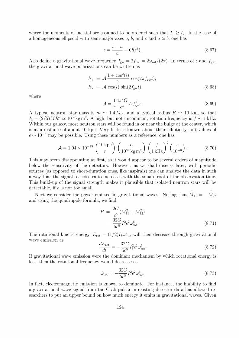
where the moments of inertial are assumed to be ordered such that I1 ≥ I2. In the case ofa homogeneous ellipsoid with semi-major axes a, b, and c and a ' b, one has

ε =b− aa

+O(ε2). (8.67)

Also define a gravitational wave frequency fgw = 2frot = 2ωrot/(2π). In terms of ε and fgw,the gravitational wave polarizations can be written as

h+ = A 1 + cos2(ι)

2cos(2πfgwt),

h× = A cos(ι) sin(2fgwt), (8.68)

where

A =1

r

4π2G

c4I3f

2gwε. (8.69)

A typical neutron star mass is m ' 1.4M, and a typical radius R ' 10 km, so thatI3 = (2/5)MR2 ' 1038kg m2. A high, but not uncommon, rotation frequency is f ∼ 1 kHz.Within our galaxy, most neutron stars will be found in or near the bulge at the center, whichis at a distance of about 10 kpc. Very little is known about their ellipticity, but values ofε ∼ 10−6 may be possible. Using these numbers as a reference, one has

A = 1.04× 10−25

(10 kpc

r

) (I3

1038 kg m2

) (f

1 kHz

)2 ( ε

10−6

). (8.70)

This may seem disappointing at first, as it would appear to be several orders of magnitudebelow the sensitivity of the detectors. However, as we shall discuss later, with periodicsources (as opposed to short-duration ones, like inspirals) one can analyze the data in sucha way that the signal-to-noise ratio increases with the square root of the observation time.This build-up of the signal strength makes it plausible that isolated neutron stars will bedetectable, if ε is not too small.

Next we consider the power emitted in gravitational waves. Noting that ¨M11 = − ¨M22

and using the quadrupole formula, we find

P =2G

c5〈 ¨M2

11 + ¨M212〉

=32G

5c5I2

3 ε2ω6

rot. (8.71)

The rotational kinetic energy, Erot = (1/2)I3ω2rot, will then decrease through gravitational

wave emission asdErot

dt= −32G

5c5I2

3 ε2ω6

rot. (8.72)

If gravitational wave emission were the dominant mechanism by which rotational energy islost, then the rotational frequency would decrease as

ωrot = −32G

5c5I2

3 ε2ω5

rot. (8.73)

In fact, electromagnetic emission is known to dominate. For instance, the inability to finda gravitational wave signal from the Crab pulsar in existing detector data has allowed re-searchers to put an upper bound on how much energy it emits in gravitational waves. Given

124

the spin-down rate of the pulsar (which is known from radio observations) and the sensitivityof the detectors, it was determined that no more than 6% of the Crab’s rotational energyloss goes into gravitational radiation, or else a gravitational wave signal should have beenseen.47

C. Mapping the geometry of the Universe with gravitational waves

We have seen how standard candles, such as Type Ia supernovae, are standard candles :their luminosity distance can be determined (with some error) from their brightness, andtheir redshift can be measured separately. With a sufficient number of standard candles,one can use the relation

DL = DL(z;H0,ΩM,ΩR,ΩDE,Ωk, w) (8.74)

to constrain the cosmological parameters ΩM etc. However, standard candles are only asreliable as the calibration of their intrinsic luminosity, which depends on a “cosmic distanceladder” of other kinds of sources.

The observation of gravitational waves from the inspiral and merger of compact objectswill obviate the need for a cosmic distance ladder. Schematically, the strain such signalsinduce in a detector looks like

h(t) =M5/3

c

DL

A(θ, φ, ψ, ι) cos(Φ(t)). (8.75)

The angles θ and φ give the sky position of the source, ψ is the polarization angle, and ι isthe inclination angle of the orbital plane. If at least one of the compact objects is a neutronstar then the merger will produce electromagnetic radiation. Indeed, short, hard gammaray bursts (GRBs) – the brightest events since the Big Bang – are believed to be causedby merging binary neutron stars. If a gamma ray bursts is observed electromagnetically incoincidence with the gravitational wave observation of a binary neutron star coalescence,then it will be natural to associate the two events. In many cases the sky location of agamma ray burst can be determined, so that θ and φ will be known. It is believed that thegamma ray emission of GRBs happens in tight beams perpendicular to the inspiral plane; ifthis is so then one can assume ι ' 0, in which case ψ also disappears from the expression forA. However, with a network of detectors one can measure ι and ψ with reasonable accuracy,so that further assumptions are not necessary. This way, A is known. When measuring theamplitude of the signal, one would then still need to disentangleMc and DL. However, fromthe expression (8.29) we see that, to leading order in small parameters, the phasing Φ(t) iscompletely determined by Mc. Hence, by studying the time evolution of the signal’s phaseone can measure Mc. With θ, φ, ψ, ι, and Mc known, one can then also determine DL bymeasuring the amplitude of the signal.

Another possibility is using binary supermassive black holes observed by the space-basedLISA. In that case the signals will be in band for a year or so, during which time LISAmoves about the Sun. This motion Doppler-modulates the gravitational waveform, from

47 The actual fraction is likely to be much lower, but this was one of the first important results fromgravitational wave astronomy.

125

which (θ, φ, ι, ψ) can be obtained without the need for an electromagnetic counterpart, andalso Mc and DL. If the determination of the sky position is sufficiently accurate that thehost galaxy can be determined, then once again z can be measured.

Inspiral events are self-calibrating ; there is no need to take recourse to other kinds ofsources to determine their luminosity distance DL. With sky position known, one can alsofind out in which galaxy the inspiral occurred. The redshift z of a galaxy can be measuredwith high accuracy by looking at its spectrum. Thus, DL and z can be inferred independently,and binary neutron star inspiral are standard candles. Because their frequencies happen tofall in the range of audible sound, they are often referred to as standard sirens.

In the rest of this chapter we will discuss how standard sirens could be used to determinethe geometry of the Universe. First we need to know how gravitational waves propag-ate through a FLRW Universe. Previously we linearized general relativity around a flat(Minkowksi) background; here we need to linearize around a FLRW spacetime. We will notgo into details here, but in fact the derivation follows closely what we did before, exceptthat ηµν is replaced by the background metric gµν . One defines

hµν = hµν −1

2gµνh, (8.76)

with h = gµνhµν . The equivalent of the harmonic gauge condition is

∇ν hµν = 0, (8.77)

where ∇ is the covariant derivative adapted to the background metric. The linearizedvacuum Einstein equations then take the form

∇ρ∇ρhµν = 0. (8.78)

One can also impose a TT gauge, in which hµν = hµν .It is not difficult t show that in a (matter-dominated) FLRW Universe, a general spher-

ically symmetric solution of Eq. (8.78) that falls of as 1/r approximately takes the form

hµν '1

ra(t)Hµν(t− r/c). (8.79)

Eq. (8.79) tells us that in the expressions for the inspiral waveforms, Eqns. (8.28), weonly need to replace 1/r by 1/(a(t) r) to take into account the effect of the cosmologicalbackground.

To fully understand the effect of propagation through a FLRW spacetime, let us first lookat what happens near the source. Define the local wave zone as a region close enough to thesource that the expansion of the Universe can be neglected, but sufficiently far so we arenot in the strong-field regime and the quadrupole approximation holds. In the local wavezone, one has

h+(tem) = h0(tem,ret)1 + cos2(ι)

2cos

[2π

∫ tret,em

dt′emfgw,em(t′em)

]h×(tem) = h0(tem,ret) cos(ι) sin

[2π

∫ tret,em

dt′emfgw,em(t′em)

], (8.80)

126

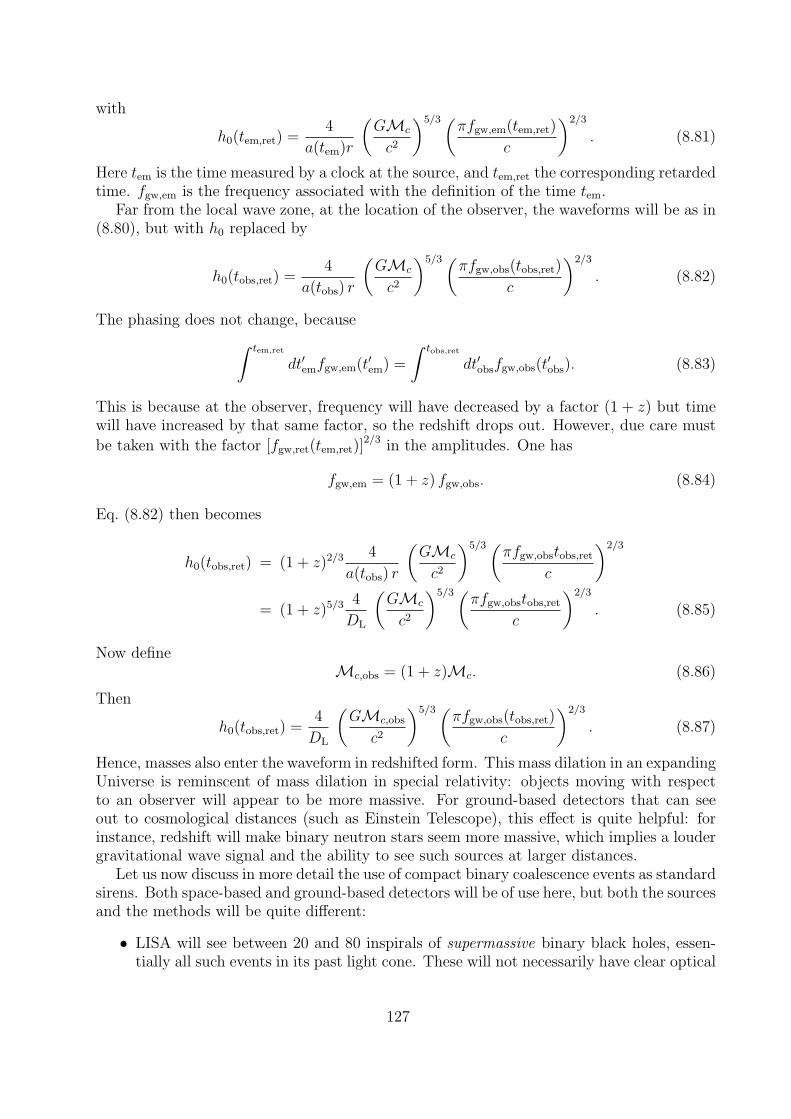
with

h0(tem,ret) =4

a(tem)r

(GMc

c2

)5/3(πfgw,em(tem,ret)

c

)2/3

. (8.81)

Here tem is the time measured by a clock at the source, and tem,ret the corresponding retardedtime. fgw,em is the frequency associated with the definition of the time tem.

Far from the local wave zone, at the location of the observer, the waveforms will be as in(8.80), but with h0 replaced by

h0(tobs,ret) =4

a(tobs) r

(GMc

c2

)5/3(πfgw,obs(tobs,ret)

c

)2/3

. (8.82)

The phasing does not change, because∫ tem,ret

dt′emfgw,em(t′em) =

∫ tobs,ret

dt′obsfgw,obs(t′obs). (8.83)

This is because at the observer, frequency will have decreased by a factor (1 + z) but timewill have increased by that same factor, so the redshift drops out. However, due care must

be taken with the factor [fgw,ret(tem,ret)]2/3 in the amplitudes. One has

fgw,em = (1 + z) fgw,obs. (8.84)

Eq. (8.82) then becomes

h0(tobs,ret) = (1 + z)2/3 4

a(tobs) r

(GMc

c2

)5/3(πfgw,obstobs,ret

c

)2/3

= (1 + z)5/3 4

DL

(GMc

c2

)5/3(πfgw,obstobs,ret

c

)2/3

. (8.85)

Now defineMc,obs = (1 + z)Mc. (8.86)

Then

h0(tobs,ret) =4

DL

(GMc,obs

c2

)5/3(πfgw,obs(tobs,ret)

c

)2/3

. (8.87)

Hence, masses also enter the waveform in redshifted form. This mass dilation in an expandingUniverse is reminscent of mass dilation in special relativity: objects moving with respectto an observer will appear to be more massive. For ground-based detectors that can seeout to cosmological distances (such as Einstein Telescope), this effect is quite helpful: forinstance, redshift will make binary neutron stars seem more massive, which implies a loudergravitational wave signal and the ability to see such sources at larger distances.

Let us now discuss in more detail the use of compact binary coalescence events as standardsirens. Both space-based and ground-based detectors will be of use here, but both the sourcesand the methods will be quite different:

• LISA will see between 20 and 80 inspirals of supermassive binary black holes, essen-tially all such events in its past light cone. These will not necessarily have clear optical

127

counterparts48, so that the sky location (needed for measurement of redshift throughidentification of the host galaxy) will need to be determined from the gravitationalwave signal itself. Fortunately LISA’s motion around the Sun causes a Doppler mod-ulation of the signal, which allows for rather good pointing accuracy. Even so, studieshave determined that a source will have to be at a redshift z . 1 for host identificationto be possible. It is expected that the instrument will see about one source per yearthat is close enough to be used for cosmography.

• Advanced ground-based instruments will see tens to hundreds of coalescences involvingat least one neutron star. If the associated gamma ray burst is observed then the hostgalaxy and the redshift can be established. Einstein Telescope will see in the order ofa million such coalescences out to cosmological distances (see Fig. 31); in the courseof several years, a thousand of these may allow for redshift measurement.

Figure 31: The distance and redshift reach of Einstein Telescope. M is total mass while ν =m1m2/M is the so-called symmetric mass ratio; equal component mass systems have ν = 0.25.The red solid curves give distances as functions of physical mass M , the blue dash-dotted ones asfunctions of the observed mass (1 + z)M .

As discussed above, cosmography requires an independent measurement of redshift z andluminosity distance DL. The latter is to be measured from the gravitational wave signal.The Fisher matrix formalism which we discussed earlier will give us an indication of how

48 By the time a supermassive binary black hole will be orbiting with sufficient frequency to be in the LISAband, a common accretion disk will have formed. At merger, several percent of the binary’s mass/energywill be radiated away in a matter of hours. This will cause a sudden change in the Newtonian potential,which determines the orbits of matter particles in the accretion disk. The change will lead to a shockwave through the disk, and the attendant heating may cause a sufficiently distinct electromagnetic signal.However, the accretion disk will be so large that such a signal may take several years to be generated.Even then, it may not be distinguishable from the natural variability of quasars.

128

well this can be done. Recall that the Fisher matrix Γij is defined as

Γij = (∂ih|∂jh), (8.88)

with ∂ih = ∂h/∂λi. The covariance matrix Σij = (Γij)−1 gives 1-σ uncertainties in theparameters λi, as well as their correlation coefficients:

∆λi =√

Σii,

cij =Σij

√ΣiiΣjj

, (8.89)

where no summation over repeated indices is assumed. From Eqns. (8.80), (8.82), (8.29),and the discussion around Eq. (8.33) we see that the parameters (θ, φ, ψ, ι, r) only enter theamplitude, not the phase; hence we can expect them to be strongly correlated, at least apriori. Mc,obs also appears in the amplitude, but it can be measured from the phase withgood accuracy. Since the scheme outlined above requires knowledge of sky position, we mayassume that (θ, φ) are known. In the case of LISA, the orientation of the source will appearto be changing as the probes move around the Sun, allowing for a determination of (ψ, ι).For ground-based detectors, if GRBs are indeed strongly beamed49 then ι ' 0, in which caseψ drops out of the waveform, as radiation emitted perpendicularly to the inspiral plane iscircularly polarized. Even if this is too strong an assumption, with a network of detectorsseeing the source with different apparent orientations, ι and ψ can be disentangled.

Whatever parameters are known by other means need not be included in (8.88), whichonly pertains to measurements using the gravitational waveform. Hence (θ, φ) are absentfrom (8.88); (ι, φ) will be approximately zero in the case of GRBs, and not that stronglycorrelated in the case of LISA; and Mc,obs can be obtained from the phasing. Very roughlythen, we may then treat the Fisher matrix as if it is block-diagonal, with DL in one block.In that case,

∆DL ∼1√

(∂DLh|∂DL

h). (8.90)

Note that∂h

∂DL

= − 1

DL

h, (8.91)

so∆DL

DL

∼ 1√(h|h)

=1

ρ, (8.92)

with ρ the signal-to-noise ratio.First let’s assume we only want to determine H0, the Hubble parameter at the current

era. Ignoring correlations with the other cosmological parameters50 (ΩM, ΩDE, w),

∆DL =

∣∣∣∣∂DL

∂H0

∣∣∣∣ ∆H0. (8.93)

49 The estimated total beaming angle is ∼ 40. Note that this is not a stereal angle; indeed, the associatedsurface area on the unit sphere is only about 3%.

50 In this section, for simplicity we will assume ΩR = Ωk = 0.

129

From Eqns. (2.69), (2.43), and (8.91), we see that

∆H0

H0

=∆DL

DL

. (8.94)

First consider ground-based detectors. Most of its sources will be close to the angle-averagedhorizon distance, as larger distances correspond to larger volumes and hence to a highersource rate. This that for the majority of sources, ρ will be not much larger than thethreshold SNR required for detection; for concreteness, ρ ∼ 10. Then the above expressiontogether with (8.92) implies that with a single source, H0 can be measured with a relat-ive accuracy of 10%. However, with N sources, the uncertainty will go down roughly as√N . The Advanced LIGO-Virgo network is expected to see about 40 BNS events per year.

Suppose that, over the course of several years, there will be 10 sources with a sufficientlydistinct electromagnetic counterpart (not necessarily a gamma ray burst; there could bea non-beamed afterglow); then we gain about a factor of 3, leading to ∆H0/H0 ∼ 3%.Einstein Telescope is expected to see ∼ 1000 identifiable sources over the course of severalyears; again assuming an SNR close to threshold (ρ ∼ 10), we get ∆H0/H0 ∼ 0.3%. Asexplained above, in the case of LISA we may have only one source for which a redshift canbe determined. On the other hand, this must then be a relatively close-by source, withz . 1. The SNR will depend sensitively on sky position and orientation, but ρ ' 1000 isreasonable. Thus, ∆H0/H0 ∼ 0.1% in that case.

One can also assume that, say, (H0,ΩM,ΩDE) have already been determined by othermeans and try to measure the dark energy equation-of-state parameter w. Again assumingno correlations among the cosmological parameters,

∆DL =

∣∣∣∣∂DL

∂w

∣∣∣∣ ∆w, (8.95)

or

∆w = DL

∣∣∣∣∂DL

∂w

∣∣∣∣−1∆DL

DL

. (8.96)

For definiteness, let us assume the true value of w to be w = −1, corresponding to acosmological constant. We first consider LISA. For a source at z ∼ 0.5, one has DL ' 3 Gpcand |∂DL/∂w| ∼ 500 Mpc. Again taking ∆DL/DL ∼ ρ ∼ 103, this leads to ∆w/|w| ∼ 0.6%.Sources in ET will be spread out in redshift up to z ∼ 2, but we can make a back-of-the-envelope estimate. The ET sources that contribute the most to estimates of cosmologicalparameters also happen to be roughtly at z ∼ 0.5, with an SNR of about 20. This leadsto ∆w/|w| ∼ 30% for an individual source. Assuming N = 1000 sources and dividing by√N , we get ∆w/|w| ∼ 1%, which is actually very close to what was found in more in-depth

studies.In reality these uncertainties will be larger because of weak lensing. The matter between

source and observer acts as a lens, leading to magnification or demagnification. Light andgravitational waves are affected in exactly the same way: gravitons and photons both movealong lightlike geodesics! This has the effect of corrupting measurements of DL. For theAdvanced detectors this will not be much of a problem, since their sources will be relativelyclose-by (up to about 1 Gpc). However, for sources up to z ∼ 1 (about 3 Gpc), the effecton distance measurements has been estimated to be at the 3− 5% level. Since this error isindependent of the uncertainties due to instrumental noise, it can be combined in quadrature

130

with ∆DL/DL: [∆DL

DL

]total

=

([∆DL

DL

]2

noise

+

[∆DL

DL

]2

lensing

)1/2

. (8.97)

If, for definiteness, we assume a 4% error, then the above LISA estimates will be completelydominated by weak lensing errors: [∆H0/H0]total ∼ 4% and [∆w]total ∼ 23%. Fortunately,it may be possible to at least partially subtract these effects. Other than (de)magnification,lensing also causes deformations in galaxy images (causing them to be banana-shaped ratherthan elliptical). By making maps of these deformations one can infer the distribution ofmatter along the line of sight, model the effect of weak lensing, and at least partially subtractit. Note that weak lensing will be far less of a problem for ET, because of large numberstatistics. Repeating the rough estimate above but with [∆DL/DL]total = (0.042+0.052)1/2 '6.4%, with 1000 sources one gets an error of 1.2%, barely different from the value withoutweak lensing.

Of course we will want to measure all four parameters H0, ΩM, ΩDE, and w, which willrequire at least four measurements. Hence, this is something one can not do with LISA alone– although LISA observations can of course be combined with those of other gravitational-wave observatories. Advanced LIGO-Virgo could in principle be used, but the number ofsources will be too low to independently measure all parameters. For (ΩM,ΩDE, w) one canalways use values obtained by electromagnetism. However, as explained above, this wouldthen make the results dependent on the cosmic distance ladder, which is undesirable. ButEinstein Telescope will be suitable. One could first get a high-quality measure of the Hubbleconstant by using fairly nearby sources that are unaffected by weak lensing and have a highSNR. Careful studies have shown that with only 50 sources up to z = 0.5, one could measureH0 with a relative error of 0.5%. Next, using the rest of the sources and keeping the value ofH0 fixed51, one could find the values of (ΩM,ΩDE, w) by making a best fit of the measuredvalues of DL against z. To estimate uncertainties, one could create simulated “catalog”of sources at different redshifts zi, i = 1, . . . , 1000, and assigning to each a “measured”

distance D(i)L = DL(zi) + δD

(i)L . Here DL(zi) is the true distance, while the “measurement

error” δD(i)L is drawn from a Gaussian distribution with a width ∆DL(z), computed using

the Fisher matrix formalism. One then fits the measured distances to the redshift, leadingto “measured values” (ΩM), ΩDE, w for the cosmological parameters. Having repeated thismany times with many different simulated catalogs, one gets a distribution for these values,of which the variance can be computed. This is what is shown in Fig. 32.

The result for, e.g., the dark energy measurement is competitive with projections forfuture, dedicated dark energy missions, where 3.5-11% uncertainty is expected. However,we reiterate that gravitational wave standard sirens are self-calibrating and have no needfor an elaborate cosmic distance ladder, circumventing possible unknown systematic errors.What they will tell us about the geometry of the Universe is guaranteed to be correct withinthe stated statistical errors.

51 As it turns out, simply measuring (H0,ΩM,ΩDE, w) all at once leads to intolerably large uncertainties;measuring H0 separately solves the problem by avoiding a degeneracy.

131

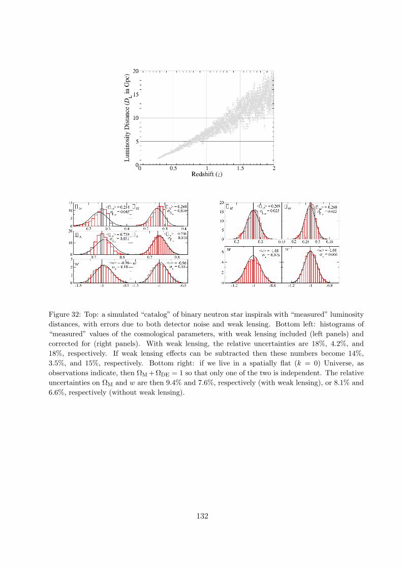
Figure 32: Top: a simulated “catalog” of binary neutron star inspirals with “measured” luminositydistances, with errors due to both detector noise and weak lensing. Bottom left: histograms of“measured” values of the cosmological parameters, with weak lensing included (left panels) andcorrected for (right panels). With weak lensing, the relative uncertainties are 18%, 4.2%, and18%, respectively. If weak lensing effects can be subtracted then these numbers become 14%,3.5%, and 15%, respectively. Bottom right: if we live in a spatially flat (k = 0) Universe, asobservations indicate, then ΩM + ΩDE = 1 so that only one of the two is independent. The relativeuncertainties on ΩM and w are then 9.4% and 7.6%, respectively (with weak lensing), or 8.1% and6.6%, respectively (without weak lensing).

132