I do not know what I may appear to the world; but to myself I seem to have been only likea boy playing on the seashore, and diverting myself in now and then finding of a smootherpebble or a prettier shell than ordinary, whilst the great ocean of truth lay all undiscovered

before me.

- Sir Isaac Newton

University of Alberta

Game-Independent AI Agents for Playing Atari 2600 ConsoleGames

by

Yavar Naddaf

A thesis submitted to the Faculty of Graduate Studies and Researchin partial fulfillment of the requirements for the degree of

Master of Science

Department of Computing Science

c©Yavar NaddafSpring 2010

Edmonton, Alberta

Permission is hereby granted to the University of Alberta Libraries to reproduce single copies ofthis thesis and to lend or sell such copies for private, scholarly or scientific research purposes only.

Where the thesis is converted to, or otherwise made available in digital form, the University ofAlberta will advise potential users of the thesis of these terms.

The author reserves all other publication and other rights in association with the copyright in thethesis, and except as herein before provided, neither the thesis nor any substantial portion thereofmay be printed or otherwise reproduced in any material form whatever without the author’s prior

written permission.

Examining Committee

Michael Bowling, Department of Computing Science

Richard Sutton, Department of Computing Science

Vadim Bulitko, Department of Computing Science

Sean Gouglas, Department of History & Classics

Abstract

This research focuses on developing AI agents that play arbitrary Atari 2600 console games

without having any game-specific assumptions or prior knowledge. Two main approaches are

considered: reinforcement learning based methods and search based methods. The RL-based

methods use feature vectors generated from the game screen as well as the console RAM

to learn to play a given game. The search-based methods use the emulator to simulate the

consequence of actions into the future, aiming to play as well as possible by only exploring

a very small fraction of the state-space.

To insure the generic nature of our methods, all agents are designed and tuned using four

specific games. Once the development and parameter selection is complete, the performance

of the agents is evaluated on a set of 50 randomly selected games. Significant learning is

reported for the RL-based methods on most games. Additionally, some instances of human-

level performance is achieved by the search-based methods.

Acknowledgements

I have been very fortunate to have an enjoyable and fruitful learning experience here in

University of Alberta, and for this I am most grateful to my supervisor, Michael Bowling.

He has provided me with the opportunity to work on a research topic that I am truly

passionate about, given me enough academic freedom to experiment and learn on my own,

and yet he has always been there to guide me when I was lost and confused.

I am very thankful to my fellow graduate students who have generously and patiently

shared their knowledge and expertise and have been instrumental for the completion of this

thesis. In particular, I would like to thank Marc Lanctot and Chris Rayner for sharing their

knowledge and getting me started with the Atari 2600 hardware and the emulation tools,

Mohammad Shafiei for sharing his insights on the concepts behind the UCT algorithm,

and Michael Johanson for offering his expertise on running batch simulations on computer

clusters. Our late night discussions with Amir-Massoud Farahmand have been some of the

best learning experiences I have had through the last two years. I am very grateful to him,

who has been both an inspiring colleague and a good friend.

I am indebted to the team behind Stella, the Atari 2600 emulator, for releasing their

work as open-source and allowing me to build my toolset on top of their code. I would

also like to thank Richard Sutton and the RLAI group for releasing the source code of their

Tile-Coding and Sarsa(λ) implementations. I hope that releasing my own code base as

open-source will be similarly beneficial to other researchers and hobbyists.

Table of Contents

1 Introduction 11.1 Problem Statement . . . . . . . . . . . . . . . . . . . . . . . . . . . . . . . . . 11.2 Motivation . . . . . . . . . . . . . . . . . . . . . . . . . . . . . . . . . . . . . 3

1.2.1 Artificial Intelligence in Games . . . . . . . . . . . . . . . . . . . . . . 31.2.2 Atari 2600: an Attractive Platform for AI Research . . . . . . . . . . 41.2.3 More Generic Evaluation of AI Methods . . . . . . . . . . . . . . . . . 5

1.3 Related Work . . . . . . . . . . . . . . . . . . . . . . . . . . . . . . . . . . . . 51.4 Contributions . . . . . . . . . . . . . . . . . . . . . . . . . . . . . . . . . . . . 71.5 Thesis Outline . . . . . . . . . . . . . . . . . . . . . . . . . . . . . . . . . . . 8

2 Reinforcement Learning Agents using Gradient Descent Sarsa(λ) 92.1 Preliminaries . . . . . . . . . . . . . . . . . . . . . . . . . . . . . . . . . . . . 9

2.1.1 Reinforcement Learning . . . . . . . . . . . . . . . . . . . . . . . . . . 102.1.2 Function Approximation . . . . . . . . . . . . . . . . . . . . . . . . . . 112.1.3 Gradient-Descent Sarsa(λ) with Linear Function Approximation . . . 122.1.4 Optimistic Initialization . . . . . . . . . . . . . . . . . . . . . . . . . . 132.1.5 Tile-Coding . . . . . . . . . . . . . . . . . . . . . . . . . . . . . . . . . 13

2.2 A Generic RL-based Agent for Atari 2600 Games . . . . . . . . . . . . . . . . 152.3 Feature Vector Generation based on Basic Abstraction of the ScreenShots

(BASS) . . . . . . . . . . . . . . . . . . . . . . . . . . . . . . . . . . . . . . . 162.4 Feature Vector Generation based on Detecting Instances of Classes of Objects

(DISCO) . . . . . . . . . . . . . . . . . . . . . . . . . . . . . . . . . . . . . . . 202.4.1 Background Detection . . . . . . . . . . . . . . . . . . . . . . . . . . . 212.4.2 Blob Extraction . . . . . . . . . . . . . . . . . . . . . . . . . . . . . . 212.4.3 Class Discovery . . . . . . . . . . . . . . . . . . . . . . . . . . . . . . . 222.4.4 Class Instance Detection . . . . . . . . . . . . . . . . . . . . . . . . . . 262.4.5 Feature Vector Generation . . . . . . . . . . . . . . . . . . . . . . . . . 26

2.5 Feature Vector Generation based on Console Memory (RAM) . . . . . . . . . 292.6 Parameter Search . . . . . . . . . . . . . . . . . . . . . . . . . . . . . . . . . . 312.7 Experimental Results on the Training Games . . . . . . . . . . . . . . . . . . 322.8 Discussion . . . . . . . . . . . . . . . . . . . . . . . . . . . . . . . . . . . . . . 33

2.8.1 Sensitivity to the Learning Rate (α) . . . . . . . . . . . . . . . . . . . 332.8.2 Delayed Rewards and Delayed Consequences . . . . . . . . . . . . . . 352.8.3 Complex Value Function . . . . . . . . . . . . . . . . . . . . . . . . . . 362.8.4 Non-Markovian States . . . . . . . . . . . . . . . . . . . . . . . . . . . 372.8.5 Challenge of Playing Arbitrary Games . . . . . . . . . . . . . . . . . 38

3 Search-based Methods 393.1 Generating a State-Action Tree . . . . . . . . . . . . . . . . . . . . . . . . . . 393.2 A Generic Search-based Agent . . . . . . . . . . . . . . . . . . . . . . . . . . 403.3 Full-Tree Search . . . . . . . . . . . . . . . . . . . . . . . . . . . . . . . . . . 40

3.3.1 Avoiding Death: A Simple Heuristic . . . . . . . . . . . . . . . . . . . 423.3.2 Choosing Parameters . . . . . . . . . . . . . . . . . . . . . . . . . . . . 423.3.3 Results for the Training Games . . . . . . . . . . . . . . . . . . . . . . 44

3.4 UCT: Upper Confidence Bounds applied to Trees . . . . . . . . . . . . . . . . 453.4.1 Overview of the Algorithm . . . . . . . . . . . . . . . . . . . . . . . . 453.4.2 Setting the UCT Bias Constant . . . . . . . . . . . . . . . . . . . . . . 463.4.3 Avoiding Death in UCT . . . . . . . . . . . . . . . . . . . . . . . . . . 483.4.4 Results on the Training Games . . . . . . . . . . . . . . . . . . . . . . 49

3.5 Discussion . . . . . . . . . . . . . . . . . . . . . . . . . . . . . . . . . . . . . . 50

4 Evaluation Method and Experimental Results 514.1 Training and Test Games . . . . . . . . . . . . . . . . . . . . . . . . . . . . . 514.2 Emulation Software . . . . . . . . . . . . . . . . . . . . . . . . . . . . . . . . . 514.3 Experimental Setup . . . . . . . . . . . . . . . . . . . . . . . . . . . . . . . . 524.4 Results on the Test Games . . . . . . . . . . . . . . . . . . . . . . . . . . . . 524.5 Impact of Game Properties on Agents Performance . . . . . . . . . . . . . . . 55

5 Conclusion and Future Work 59

A Video Game Terminology 62

B Description of the Training Games 63B.1 Asterix . . . . . . . . . . . . . . . . . . . . . . . . . . . . . . . . . . . . . . . . 63B.2 Freeway . . . . . . . . . . . . . . . . . . . . . . . . . . . . . . . . . . . . . . . 63B.3 Seaquest . . . . . . . . . . . . . . . . . . . . . . . . . . . . . . . . . . . . . . . 64B.4 Space Invaders . . . . . . . . . . . . . . . . . . . . . . . . . . . . . . . . . . . 64

C Atari 2600 Technical Specifications 65

Bibliography 66

List of Tables

2.1 Sarsa(λ) parameters . . . . . . . . . . . . . . . . . . . . . . . . . . . . . . . . 322.2 Sarsa(λ) results on the training games . . . . . . . . . . . . . . . . . . . . . . 332.3 Sarsa(λ) parameters of iDBD in RAM-agent . . . . . . . . . . . . . . . . . . . 342.4 Meta-learning parameters of iDBD in RAM-agent . . . . . . . . . . . . . . . . 35

3.1 Full-tree search results on the training games . . . . . . . . . . . . . . . . . . 443.2 UCT results on the training games . . . . . . . . . . . . . . . . . . . . . . . . 50

4.1 Experimental Results: Detailed . . . . . . . . . . . . . . . . . . . . . . . . . . 534.1 Experimental Results: Detailed . . . . . . . . . . . . . . . . . . . . . . . . . . 544.2 Experimental Results: Summary . . . . . . . . . . . . . . . . . . . . . . . . . 554.3 Search-based agents with human-level performance . . . . . . . . . . . . . . . 554.4 Test Games Properties . . . . . . . . . . . . . . . . . . . . . . . . . . . . . . . 564.4 Test Games Properties . . . . . . . . . . . . . . . . . . . . . . . . . . . . . . . 574.5 Effect of delayed rewards on performance of the agents . . . . . . . . . . . . . 58

List of Figures

1.1 Screenshots of four Atari 2600 games . . . . . . . . . . . . . . . . . . . . . . . 2

2.1 Pseudocode for linear gradient-descent Sarsa(λ) with binary feature vectors . 142.2 A generic RL-based agent . . . . . . . . . . . . . . . . . . . . . . . . . . . . . 152.3 A visualization of screenshot abstraction in BASS . . . . . . . . . . . . . . . . 182.4 BASS Pseudocode . . . . . . . . . . . . . . . . . . . . . . . . . . . . . . . . . 192.5 Sample screenshots from the training games Freeway and Seaquest . . . . . . 202.6 Pseudocode for histogram-based background detection . . . . . . . . . . . . . 222.7 Blob Extraction Pseudocode . . . . . . . . . . . . . . . . . . . . . . . . . . . . 232.8 Background detection and blob extraction for the games Freeway and Seaquest 242.9 Class Discovery Pseudocode . . . . . . . . . . . . . . . . . . . . . . . . . . . . 252.10 Discovered classes in the game Freeway . . . . . . . . . . . . . . . . . . . . . 252.11 Pseudocode code for class instance detection and calculating instance velocities 262.12 Class instances detected in sample screens of Freeway and Seaquest . . . . . . 272.13 Feature vector generation for the game Freeway: simple . . . . . . . . . . . . 282.14 Feature vector generation for the game Freeway: complex . . . . . . . . . . . 292.15 DISCO Pseudocode . . . . . . . . . . . . . . . . . . . . . . . . . . . . . . . . 302.16 Feature Vector Generation based on Console Memory (RAM) . . . . . . . . . 322.17 Learning progress for the RL-agents on the training games . . . . . . . . . . . 342.18 A demonstration of the Non-Markovian property of an Atari 2600 game screen 37

3.1 Illustration of the state-action tree generation using the emulator . . . . . . . 413.2 A generic search-based agent . . . . . . . . . . . . . . . . . . . . . . . . . . . 423.3 Full-tree search with the avoiding death heuristic. . . . . . . . . . . . . . . . . 433.4 UCT Pseudocode . . . . . . . . . . . . . . . . . . . . . . . . . . . . . . . . . . 473.5 Conceptual graph of how UCT expands the state-action tree . . . . . . . . . 48

C.1 The Atari 2600 Video Computer System . . . . . . . . . . . . . . . . . . . . . 65

Chapter 1

Introduction

Atari 2600 was a popular second generation game console, released in 1977. With a 1.19

MHz CPU, 128 bytes of RAM , and no frame buffer, it offers minimal hardware capabilities

compared to a modern game console. Nonetheless, Atari 2600 programmers learned to push

the capabilities of this limited hardware and there were numerous shooter, action-adventure,

and puzzle games developed for the platform. Many popular arcade games, including Space

Invaders, Pac-Man, and Donkey Kong were also ported to the Atari 2600. Atari shipped

over 25 million units of the console, which became the dominant console of the second

generation of game consoles. A rich library of over 900 game titles, simple 2D graphics, and

availability of open-source emulation software make the Atari 2600 an attractive platform

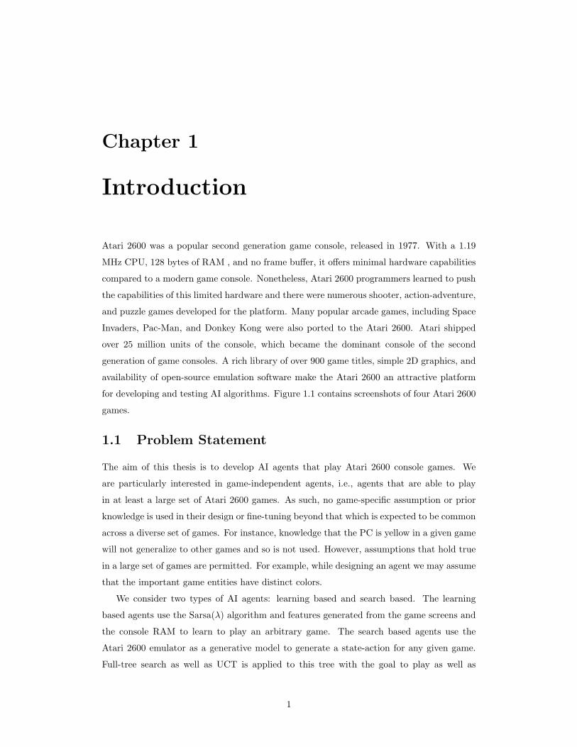
for developing and testing AI algorithms. Figure 1.1 contains screenshots of four Atari 2600

games.

1.1 Problem Statement

The aim of this thesis is to develop AI agents that play Atari 2600 console games. We

are particularly interested in game-independent agents, i.e., agents that are able to play

in at least a large set of Atari 2600 games. As such, no game-specific assumption or prior

knowledge is used in their design or fine-tuning beyond that which is expected to be common

across a diverse set of games. For instance, knowledge that the PC is yellow in a given game

will not generalize to other games and so is not used. However, assumptions that hold true

in a large set of games are permitted. For example, while designing an agent we may assume

that the important game entities have distinct colors.

We consider two types of AI agents: learning based and search based. The learning

based agents use the Sarsa(λ) algorithm and features generated from the game screens and

the console RAM to learn to play an arbitrary game. The search based agents use the

Atari 2600 emulator as a generative model to generate a state-action for any given game.

Full-tree search as well as UCT is applied to this tree with the goal to play as well as

1

(a) Asterix (b) Freeway

(c) Seaquest (d) Space Invaders

Figure 1.1: Screenshots of four Atari 2600 games

2

possible by only exploring a small subset of the large state-space. We acknowledge that our

current experiments are limited to one or two specific methods from a large body of possible

approaches, and as such the observations will be limited to these specific methods.

1.2 Motivation

1.2.1 Artificial Intelligence in Games

Artificial Intelligence algorithms that can play classic or video games have been studied ex-

tensively. Research in classic games has resulted in Deep Thought for chess [Campbell et al., 2002],

Chinook for checkers [Schaeffer et al., 2005], TD-Gammon for backgammon [Tesauro, 1994],

and Polaris for poker [Bowling et al., 2009]. For AI researchers who work on solving vari-

ous games, there is a recurring question that needs to be addressed: why dedicate limited

resources to solving games instead of tackling the real-world problems in which the field of

Artificial Intelligence can contribute to the daily quality of human lives? In other words,

why spend resources on solving chess, if what we need is self-driving cars with near zero

collision rates? Why play checkers, if what we want is an intelligent maid robot that can

cook, vacuum, and wash the dishes?

The motivation for developing AI agents that can play games is threefold. First, games

offer controlled, well-understood, and easily abstracted environments, with well-defined mea-

sures of success and failure. These properties make games suitable platforms for developing

and testing AI algorithms. The methods developed and the knowledge gained from work-

ing in these controlled environments can later be applied to the real-world problems which

are generally messier and harder to measure performances, but still require the same AI

sophistication.

Additionally, games are excellent platforms for showcasing the capabilities of the latest

AI techniques to the public. In 1997, when Deep Blue defeated Garry Kasparov, a great

wave of excitement was generated among regular, non-academic people about Artificial

Intelligence. This is because people understand chess, and respect the complexity involved

in playing it well. Back in 1997, the AI community was not able to develop collision-free

autonomous cars or achieve many other longer-term goals of the field. Showcasing an agent

that mastered chess helped the public understand what the AI community was capable of

at the time.

Finally, with the recent growth of commercial video games into a multibillion-dollar

industry, there is now even more motivation for studying agents that can learn to act intelli-

gently in games [Lucas, 2009, Laird and Lent, 2000]. Non-repetitive, adaptive, interesting,

and in summary intelligent behavior offers a competitive edge for commercial games. As

the game graphics peak at image-like quality, and as the game consoles offer more and more

computational power that can be spent on complex learning algorithms, the importance of

3

better game AI will only increase.

1.2.2 Atari 2600: an Attractive Platform for AI Research

The Atari 2600 game console is an excellent platform for developing and demonstrating

AI algorithms. Bellow, we list a number of the properties that make the Atari 2600 an

attractive medium for AI research:

• Large and diverse game library: There are over 900 game titles developed for

the Atari 2600 console. These game vary from arcade-style shooter games (e.g., Space

Invaders) to complex action-adventure games (e.g., Adventure) and even board-games

(e.g., Video Chess). This enables a researcher to implement an AI method once and

then evaluate it on a large and diverse sets of games.

• Multiple sources of relatively simple features: Game consoles offer many sources

of features for learning tasks, including graphics, sounds, and even the console memory.

An advantage of the Atari 2600 over the more modern game consoles is that it offers

relatively simple features. Modern consoles generate sophisticated 3D graphics and

multi-channel surround sound. On the other hand, most Atari 2600 games have simple

2D graphics, elementary sound effects, and utilize only 128 bytes of memory. This

simplicity makes Atari 2600 games a more practical starting point for developing

general AI techniques for video games.

• Discrete and small action-space: Unlike modern consoles with multiple analogue

inputs, an Atari 2600 joystick can only capture 8 discrete directions and one action

button. Combined together, Atari 2600 games use a maximum of 18 discrete actions1.

• Free and open-source emulator: There are number of free and open-source emula-

tors for the Atari 2600, including: Stella2, z26, and PC Atari Emulator. Having access

to open-source emulation software allows researchers to develop AI agents with mini-

mal exposure to the low level details of how Atari 2600 games and hardware function.

ALE, our learning environment discussed in section 4.2, is built on top of Stella.

• High emulation speed: Since the Atari 2600 CPU runs at only 1.19 megahertz, it

can be emulated at a very high speed on a modern computer running at two to three

gigahertz. Our learning environment, ALE, can emulate games as fast as 2000 frames

per second.1The action are: Up, Down, Left, Right, Up-Left, Up-Right, Down-Left, Down-Right, Up-Fire, Down-

Fire, Left-Fire, Right-Fire, Up-Left-Fire, Up-Right-Fire, Down-Left-Fire, Down-Right-Fire, Fire, NoAc-tion.

2http://stella.sourceforge.net

4

• Generative model: As we will discuss in section 3.1, an Atari 2600 emulator can

be used as a generative model, which given a state and an action, can generate the

following state. The generative model can be used in both search-based and learning-

based methods.

• Single-player and multi-player games: In addition to single-player games, many

Atari 2600 games offer two-player modes, supported by attaching a second joystick to

the console. This makes the Atari 2600 an attractive platform for multi-agent learning.

In this thesis, however, we only focuses on single-agent learning and search.

1.2.3 More Generic Evaluation of AI Methods

Most empirical evaluation of AI algorithms is performed on a small set of problems. Each

field has a few problems that most new approaches are demonstrated on3. To evaluate a

new method, researchers often implement it on these common problems and compare the

results with the results from previous algorithms. However, evaluating a new method on one

or two problems provides little evidence of how the new method would fare in a broader and

more generic sets of experiments. In other words, showing that method A slightly improves

the results of method B on the Mountain-Car problem, does not necessarily imply that it

will also do a better job in playing Robocup-Soccer or flying a helicopter. Furthermore, to

achieve the best possible performance, an individual parameter search is often performed

for each problem. It is not always clear how much work is involved in the parameter search,

and how easily a new set of parameters can be found for a different problem.

The diverse game library available for the Atari 2600 enables us to evaluate a new

method on a large set of games, each with its own unique state dynamics and reward

signals. Furthermore, we can divide the games into a training and a test set. An AI method

is developed and tuned on the training games, and is later evaluated on the test games.

Compared to performing the parameter search and the evaluation on the same problem, this

generic evaluation method provides a better insight into how well an AI algorithm would

perform on a new and untested problem. As it will be shown in section 2.8.5, developing

an agent that can play a single Atari 2600 game can be fairly easy. What is much more

challenging is generating agents that can play a large set of different games.

1.3 Related Work

Through the last decade, there has been a growing interest in developing AI agents that

can play some aspects of video games [Lucas, 2009, Buro, 2004]. In Real-Time Strategy

(RTS) games, a few examples include: Chung et al.’s abstract strategic planning in a game

3For instance, there is Mountain-Car in the field of reinforcement learning, Blocksworld in planning, and15-puzzle in heuristic search.

5

of capture-the-flag using Monte Carlo simulations [Michael Chung, 2005], Ponsen et al.’s

unit movement control in a simplified version of Battle of Survival using Hierarchical RL

[Ponsen et al., 2006], and Ponsen’s generation of dynamic scripts for playing Wargus using

Evolutionary Algorithms [Ponsen, 2004]. Examples in First-Person Shooter (FPS) games

include Smith et al.’s RL-based approach for coordinating bots in Unreal Tournament

[Smith et al., 2007] and McPartland and Gallagher’s method for learning the navigation

task in a maze environment using Sarsa(λ) [McPartland and Gallagher, 2008]. In Com-

puter Role-Playing Games (CRPGs), Spronck et al. use dynamic scripting to learn combat

behavior in the popular Neverwinter Nights game [Spronck et al., 2006], and Cutumisu et

al. approach the same problem using a variation of Sarsa(λ) with action dependent learning

rates [Cutumisu et al., 2008].

There is also a recent interest in developing agents that can play a complete side-scrolling

arcade-style game. In 2009, two AI competitions were organized on agents that can play

entire levels of Infinite Mario, a clone of Nintendo’s popular Super Mario Bros game. The

RL 2009 Competition [Mohan and Laird, 2009] requires the agents to use reinforcement

learning to learn to play the game. The learning agents are given a state representation

containing the location of the player character (PC) and other monsters, as well as the types

of the individual tiles on the screen. The agents receive a positive reward once the level is

complete, and a small negative reward on all other states. The Mario AI Competition4, on

the other hand, does not limit the agents to a specific approach. Indeed, the participants

are encouraged to use “evolutionary neural networks, genetic programming, fuzzy logic,

temporal difference learning, human ingenuity, [and] hybrids of the above”5. Playing an

Atari 2600 game was previously attempted by Diuk et. al., who illustrated the performance

of their Object-Oriented Rmax algorithm by teaching the Player Character to pass the first

screen of the game Pitfall [Diuk et al., 2008].

A shared characteristic between all the above examples, and (to our knowledge) all

previous attempts of learning to play video games, is that each agent is designed and tuned

to play a single game. Therefore, all the essential game properties (e.g., the location of the

PC and important NPC’s, health levels, and timers) are either explicitly included in the

state representation, or can be easily extracted form it. Also, game-specific abstractions are

often performed to deal with the large state-space. Furthermore, the reward signal may be

shaped in a way to accelerate the learning.

One of the key distinctions of the methods described in this thesis is their generic nature.

The agents are expected to be able to play in at least a large set of Atari 2600 games. As

such, no game-specific assumption or prior knowledge is used in their design or fine-tuning4In association with the IEEE Consumer Electronics Society Games Innovation Conference 2009 and

with the IEEE Symposium on Computational Intelligence and Games5http://julian.togelius.com/mariocompetition2009/

6

beyond that which is expected to be common across this diverse set of games. In this

regard, this research is more closely related to the field of Domain-Independent Planning,

and more particularly General Game Playing (GGP). The aim of planning is to generate a

sequence of actions that transitions the environment from the initial state to a goal state.

Planning is domain-indipendent if there is no reliance on specific structures of a single

domain [Wilkins, 1984]. In General Game Playing, the goal is to develop agents that can play

generic, finite and discrete games [Genesereth and Love, 2005]. Both domain-independent

planning and GGP share the generic characteristic of our methods. That is, the agents

are expected to solve different problems, and use no task-specific assumptions or prior

knowledge. Also, similar to our search-based methods, they have generative models that

allow the agents to simulate the consequence of their actions.

The key difference between these domains and the problems explored in this thesis

is that both domain-independent planning and General Game Playing require an explicit

declaration of the state representation and transition in a logic-based formal language. Our

methods on the other hand only use the content of the game screen and console RAM (in

the case of learning agents) or the emulator as a black box generative model (in the case

of search-based agents). Requiring a formal definition of problems differentiates domain-

independent planning and General Game Playing from this research in two important ways.

First, the formal definition of a problem can be used as a source for generic heuristics

[Haslum et al., 2005, Clune, 2007]. Also, since the formal language is generated by human

agents, defining more complex games can become impractical. In theory, it is possible to

define and play popular arcade games like Space Invaders or River Raid in both domain-

independent planning and General Game Playing. However, in practice defining the complex

dynamics of these games in a formal language is prohibitively expensive.

1.4 Contributions

The key contributions of this thesis are as follows:

• Introducing the Atari 2600, with its diverse set of games, as an attractive platform for

developing and demonstrating game AI algorithms.

• Achieving significant learning in arbitrary Atari 2600 games using Reinforcement

Learning.

• Generating a state-action tree for any Atari 2600 game using the save-state/restore-

state features of the emulator, and achieving human-level performance in a number of

games using full-tree search and UCT.

• Employing a novel method for evaluating and comparing the player agents. The

7

development and parameter search for all agents is performed on four predetermined

games (training games). Once the agents are implemented and the required parameter

are selected, their performance is evaluated on a set of 50 randomly chosen games (test

games). To our knowledge, this is the first time that a number of game AI methods

are evaluated on such a large set of problems. Similarly, this is the first time when the

parameter search and the evaluation of AI methods are performed on two separate

sets of problems.

1.5 Thesis Outline

Two distinct approaches are taken to generate agents that can play Atari 2600 games:

RL-based (chapter 2) and Search-based (chapter 3). Each chapter includes the background

material for the algorithms applied in it, as well as the results of the introduced agents on the

training games. Chapter 4 presents the evaluation method, the experimental results on the

test games, and an analysis of how certain game properties affect the learning performance of

various methods. The thesis conclusion and a number of future directions for this research is

presented in chapter 5. Appendix A defines the video game related terminology used through

the thesis. A short description for each of the training games is provided in Appendix B.

Finally, the Atari 2600 hardware specification is presented in Appendix C.

8

Chapter 2

Reinforcement Learning Agentsusing Gradient Descent Sarsa(λ)

This chapter demonstrates how the gradient descent Sarsa(λ) algorithm with linear function

approximation can be used along with feature vectors generated from the game screen or the

console RAM to learn to play Atari 2600 games. Section 2.1 presents a brief introduction to

reinforcement learning and a number of fundamental concepts that are used within the rest

of the chapter. Section 2.2 introduces a generic, model-free, RL-based framework for playing

Atari 2600 games. Our three feature vector generation methods are explained in sections

2.3 to 2.5, followed by a description of the parameter search and experimental results of

the RL-agents on the training games in sections 2.6 and 2.7. Finally, Section 2.8 explores

a number of challenges in learning game-independent Atari 2600 games and possible future

directions for this research.

Among a large body of possible reinforcement learning methods, Sarsa(λ) is selected

for two primary reasons. First, Sarsa(λ) is a widely used algorithm that has been success-

fully applied on a large range of problems. Examples of the applications of Sarsa(λ) include

RoboCup soccer keepaway [Stone et al., 2005], control of an all-terrain robot [Luders, 2007],

and learning in 3D shooter games [McPartland and Gallagher, 2008]. Also, good perfor-

mance in linear gradient descent Sarsa(λ) has a strong dependence on features that can

estimate the value function linearly. This makes Sarsa(λ) a fitting algorithm as we explore

various game-independent feature generation methods.

2.1 Preliminaries

This section provides a brief overview of reinforcement learning and a number of funda-

mental concepts that are required for the rest of this thesis. For a through introduc-

tion to reinforcement learning please refer to Sutton and Barto’s book on the subject

[Sutton and Barto, 1998].

9

2.1.1 Reinforcement Learning

Reinforcement learning (RL) is concerned with the problem of learning via interacting with

an environment. The entity that performs the interactions and does the learning is referred

to as the agent. The entire surrounding world that the agent interacts with is called the

environment. We will be assuming that the agent interacts with the environment via a

discrete and finite set of actions.

The representation of the environment that is available to the agent is referred to as the

state, denoted by s. The states are usually assumed to have the Markov property, that is,

each state should summarize all relevant information from past interactions. The transition

function P determines how the state of the environment changes with regard to the agent

actions:

P (s, a, s′) = Pr(st+1 = s′|st = s, at = a)

A policy π is a mapping from states to actions, and determines how the agent acts in

different situations in the environment. A policy could be either deterministic, i.e., each

state s is mapped to exactly one action a, or stochastic, in which case a state s is mapped

to a vector containing the probability of taking each action in that state. The learning is

guided by a reward signal, where the agent receives the reward rt at each time step t. The

reward signal can also be either deterministic or stochastic. The aim of the learning is to

find a policy π∗ which maximizes the expected sum of discounted future rewards.

A finite Markov Decision Process (MDP) is a tuple (S,A, P,R), where S is the set of

states, A is the set of actions, P is the transition function and R is the reward function,

mapping the state at the time t (st) to a reward of rt. The value of state s under policy π,

denoted by V π(s) is the sum of the discounted rewards we expect to receive if we start in

state s and follow policy π:

V π(s) = Eπ

∞∑k=0

(γkrt+k+1|st = s)

This is a case of an infinite-horizon task, since the time steps go to infinity. If the learning

task naturally breaks into smaller sequences, the task is called episodic, and the value of a

state is the expected sum of rewards until the end of the episode:

V π(s) = Eπ

T∑k=0

(γkrt+k+1|st = s)

where T is the length of an episode. V π is often referred to as the state-value function,

since it maps a state s to its value. Alternatively, we can define an action-value function,

Qπ(s, a), which is the discounted rewards we expect to receive if we start at state s, take

action a, and then follow the policy π onward.

10

The aim of reinforcement learning is to find an optimal policy, that is, a policy that

performs better than or as good as any other policy starting from any state-action:

π∗ = arg maxπ

Qπ(s, a) for all s ∈ S, a ∈ A

While the optimal policy may not be unique, there is a unique value function corresponding

to all optimal policies. This is called the optimal value function, and is denoted by V ∗ or

Q∗. Note that if the optimal value function is known, simply acting greedily with regard to

it will give us an optimal policy :

π∗(s) = arg maxa

Q∗(s, a)

When the dynamics of the environment (P and R) are known, the optimal value function

can be calculated exactly by solving the linear system of the Bellman optimality equations.

When the complete dynamics of the environment is not known, or when solving the full

linear system is impractical due to the large state-space, there are methods that estimate

the optimal value function by interacting with the environment and looking at samples of the

state transitions and the received rewards. Section 2.1.3 presents an overview of Sarsa(λ),

the algorithm we use in our RL-based agents to estimate Q∗ based on sample interactions

with the environment.

2.1.2 Function Approximation

Many interesting reinforcement learning problems have very large state-spaces, ranging from

millions states to even much more. There are two problems associated with learning and

updating the value of each state separately in a large state-space. First, storing an individual

value V (s) for every state becomes impractical. More importantly, very little generalization

will be done. That is, if we learn that a value of a state is very high or very low, we do

not generalize this to the neighboring states. This forces us to visit each of the billions

of individual states multiple times in order to get a good estimate of its value. Function

approximation allows us to overcome both problems.

When doing function approximation, each state s is represented by a vector of values

Φ(s), known as the feature vector. The length of this vector, denoted by n, is usually much

smaller than the number of states: n� |S|. The value of state s at time step t is estimated

as a parametric function over the features of s and the current parameter vector θt:

Vt(s) = f(Φ(s), θt)

The aim of the learning now becomes finding the parameter vector θ∗, which corresponds

to an approximation of the optimal value function V ∗.

Linear functions are one of the most important and most widely used parametric func-

tions for function approximation. With a linear function, the value of a state s at time t

11

becomes:

Vt(s) =n∑i=1

θt(i)Φ(s)(i)

This can also be extended to action value functions:

Qt(s, a) =n∑i=1

θt(i)Φa(s)(i)

Here, Φa(s) is the feature vector corresponding to the (s, a) state-action pair.

We are particularly interested in the case of linear functions on binary feature vectors,

i.e., when the values of the feature vector are either 0 or 1. One advantage of a binary

feature vector is that instead of storing the complete feature vector, which may be very

large and very sparse, we only need to keep track of the indices that are 1:

Qt(s, a) =∑

i∈I(Φa(s))

θt(i) (2.1)

where I(Φa(s)) is the set of one-indices in the current feature vector Φa(s).

2.1.3 Gradient-Descent Sarsa(λ) with Linear Function Approxima-tion

Sarsa(λ) is a widely used temporal difference method that stochastically approximates the

optimal value function based on the state transition and the reward samples received from

online interaction with the environment. The original Sarsa algorithm works as follows: At

time step t, the agent is in state st. It then chooses an action at from an ε-greedy policy1 based on its current estimate of the optimal value function Qt. Consequently, the agent

receives a reward of rt and the environment transitions to state st+1. The agent then chooses

action at+1 based on the ε-greedy policy. The following temporal difference update is used

to update the estimate of the action-value function based on the given (st, at, rt, st+1, at+1)

sample:

Qt+1(st, at) = Qt(st, at) + αδ

where

δ = rt + γQt(st+1, at+1)−Qt(st, at) (2.2)

and α is the learning rate.

Sarsa(λ) extends the original Sarsa algorithm by introducing the idea of eligibility traces.

Eligibility traces allow us to update the action-value function not only for the latest (st, at)

state-action pair, but also for all the recently visited state-actions. To do this, an additional

eligibility value is stored for every state-action pair, denoted by e(s, a). At each step, the

1ε-greedy policies choose the action that maximizes the current value function with probability (1 − ε)and a random action with the probability ε. This is one solution to the well-known exploration/exploitationproblem. That is, we need to insure that while the agent exploits the current estimation of the value function,it also visits other states enough to generate an accurate estimate for their values.

12

eligibility traces of all the state-action pairs are reduced by a factor of γλ. The eligibility

trace of the latest state-action e(st, at) is then set to one 2:

et(s, a) ={

1 if s = st and a = atγλet−1(s, a) for all other state-action pairs

After each (st, at, rt, st+1, at+1) sample, δ is calculated the same as in equation 2.2. How-

ever, instead of only updating Q(st, at), all state-action pairs are updated based on their

eligibility:

Qt+1(s, a) = Qt(s, a) + αδet(s, a) for all s,a (2.3)

When doing linear function approximation, instead of keeping an eligibility value for

each state, the eligibility trace vector et keeps an eligibility trace for each item in the feature

vector. On each time step, after reducing the eligibility vector by a factor of γλ, the items

corresponding to one-indices in the current feature vector are set to one. Additionally, we

may wish to clear all the traces corresponding to all actions other than the current action

at in state st:

et = γλet−1 (2.4)

et(i) ={

1 for all i ∈ I(Φat(st))0 for all i ∈ I(Φa′(st)) and a′ 6= at

(2.5)

On each step, the following gradient-descent step is used to update the parameter vector:

θt+1 = θt + αδet (2.6)

where δ is the same as in equation 2.2 and α is the learning rate. Figure 2.1 contains the

pseudocode for gradient-descent Sarsa(λ) algorithm for an episodic task.

2.1.4 Optimistic Initialization

Optimistic initialization encourages the learning agent to explore unvisited states or unseen

features. When doing function approximation, optimistic initialization is achieved by ini-

tializing the values of the weights vector Θ to a non-zero value. If the maximum state-action

value in an MDP is known, the Θ values should be initialized such that for any state-action

pair (s, a), Q(s, a) =∑ni=1 θ(i)Φa(s)(i) is the maximum value possible.

2.1.5 Tile-Coding

Tile-coding is a method to generate binary feature vectors from multi-dimensional contin-

uous values. In its most basic form, tile-coding is simply grid partitioning of scalar values.

Each element in the partition is called a tile and it corresponds to a bit in the feature

vector. The partition itself is called a tiling. With one tiling, exactly one bit will be 1 in2The method we present here is called replacing traces. In the alternative approach, called accumulating

traces, instead of setting the trace of the latest state-action pair to 1, its value is increased by 1: et(st, at) =γλet−1(st, at) + 1

13

Assume γ (discount factor), α (learning rate), A (set of available actions), ε (explo-ration/exploitattion constant), λ are defined.Let n be the length of the feature vector

For i ∈ {1, ..., n}, θ(i) =

1n

Optimistic Initialization0 Otherwise

RL Start Episode(Φ0):

1. e = ~02. Q0(a) =

Xi∈I(Φ0,a)

θ(i) ∀a ∈ A

3. a0 = Get ε-greedy Action(Q0)4. return a0

RL Step(Φt, rt):

1. δ = rt −Qt−1(at−1)

2. Qt(a) =X

i∈I(Φt,a)

θ(i) ∀a ∈ A

3. at = Get ε-greedy Action(Qt)4. δ = δ + γQt(at)5. θ = θ + αδe6. e = γλe

7. e(i) =

1 ∀i ∈ I(Φt,at)0 ∀i ∈ I(Φt,a′) and a′ 6= at

8. return at

RL End Episode(ΦT , rT ):

1. δ = rT −QT−1(aT−1)2. θ = θ + αδe

Figure 2.1: Pseudocode for linear gradient-descent Sarsa(λ) with binary feature vectors

14

On start of the game:

1. From the emulator, receive the screen matrix X0, the RAM vector M0, and the scorereceived in the first frame r0

2. Generate a feature vector Φ0 from either X0 or M0

3. a0 = RL Start Episode(Φ0)4. Apply the action a0 via the emulator

On each time step t during the game:

1. From the emulator, receive the screen matrix Xt, the RAM vector Mt, and the scorereceived in this frame rt

2. Generate a feature vector Φt from either Xt or Mt

3. at = RL Step(Φt, rt)4. Apply the action at via the emulator

On end of the game:

1. From the emulator, receive the screen matrix XT , the RAM vector MT , and the scorereceived in this frame rT

2. Generate a feature vector ΦT from either XT or MT

3. RL End Episode(ΦT , rT )4. Restart the game through the emulator

Figure 2.2: A generic RL-based agent

the resulting feature vector, and the remaining bits will be 0. However, we can have addi-

tional tilings, placed on top of each other with some offset. With n tilings, each point in

the multi-dimensional space will be inside n tiles, and thus there will always be n non-zero

values in the resulting feature vector. Larger sized tiles allow more generalization, while

more number of tilings allow a higher resolution. The binary feature vector generated by

tile-coding the continues variables x1, x2, ..., xn is denoted as: TC(x1, x2, ..., xn)T

2.2 A Generic RL-based Agent for Atari 2600 Games

We are interested in developing agents that learn to play generic games by interacting with

them. At each time step t, the agent has access to the screenshots of the game as a matrix

of color indices Xt, the score it received during the frame rt, and whether the game has

ended. In a special case, we allow the RAM-agent to have access to the console memory in

a binary vector Mt. Aside from these, the agent is not given any additional information or

prior knowledge about a game. Once the action at is chosen by the agent, it will be carried

by the emulator and the game environment moves to the next state st+1. The learning

task is episodic. Each episode starts at the point in the game when the player is able to

start acting and ends when the game ends (e.g., the player character dies) or if we reach a

predefined maximum number of frames per episode. At the end of each episode, the game

is restarted through the emulator, and a new episode begins.

Figure 2.2 contains the pseudocode for a generic RL-based agent. While the agents pre-

15

sented in this chapter exclusively use Sarsa(λ), the methods RL Start Episode, RL Step,

and RL End Episode can be implemented using any episodic, online, reinforcement learning

algorithm.

Feature representation is a very important task in most reinforcement learning problems.

With linear function approximation, we are assuming that a meaningful value function can

be represented as a linear combination of the generated features. If this assumption does not

hold, even if the learning converges, the agent will not perform very well in the environment.

Sections 2.3 to 2.5 will present three different feature generation methods for generic Atari

2600 games. The parameter search and experimental results on the training games for each

method is discussed in Sections 2.6 and 2.7.

2.3 Feature Vector Generation based on Basic Abstrac-tion of the ScreenShots (BASS)

The first feature generation method is based on looking directly at the colored pixels on

the screen. This method is motivated by three observations of the Atari 2600 hardware and

games:

1. While the Atari 2600 hardware supports a screen resolution of 160×210, game objects

are often much larger than a few pixels. Overall, the important game events happen

in a much lower resolution3.

2. Many Atari 2600 games have a static background, with a few important objects moving

on the screen. That is, while the screen matrix is densely populated, the actual

interesting features on the screen are often sparse.

3. While the hardware can show up to 128 colors in the NTSC mode, it is limited to

only 8 colors in the SECAM mode. Consequently, most games use a few number of

distinct colors to distinguish important objects on the screen.

Based on these observations, a binary feature vector is generated by looking at the existence

of each of the eight SECAM palette colors in a lower resolution version of the screens.

We assume that a matrix of background color indices4 S, and a mapping σ[0,127]⇒[0,7]

from the NTSC color indices to the SECAM palette indices are defined. On each time step,

the feature vector generation method is given a matrix of color indices X. A new screen

matrix X is generated by removing the static background and mapping the indices to the

SECAM palette:

X(y, x) ={σ(X(y, x)) If X(y, x) 6= S(y, x)−1 Otherwise (2.7)

3This is partially due to the limited hardware capabilities of the Atari 2600 which prohibits movingthousands of small objects on the screen. Another possible reason for having relatively large objects on thescreen is to allow the players to enjoy the game with some distance from their small TV screens.

4See section 2.4.1 for the method used to detect the static background

16

The new screen matrix X is then divided into a grid of m by n blocks. For each block

Bi,j , i ∈ {1, ...,m}, j ∈ {1, ..., n} an 8-bit vector vBi,jis generated, such that:

vBi,j(c) =

{1 If color c exists in the block Bi,j0 Otherwise (2.8)

The resulting 8-bit vectors are concatenated to generate anm×n×8 bit vector vl. Informally,

what this vector captures is whether there is an object of a certain color in each part of the

screen. For instance, vl(1) = 1 indicates that there is an object with color index 1 in the

upper left corner of the screen. For example, in the case of the game Asterix, the vector vl

captures if there is a green object (which is the color of the player character), a red object

(collectable objects), or a pink object (enemy units) in each sub block of the screen. Figure

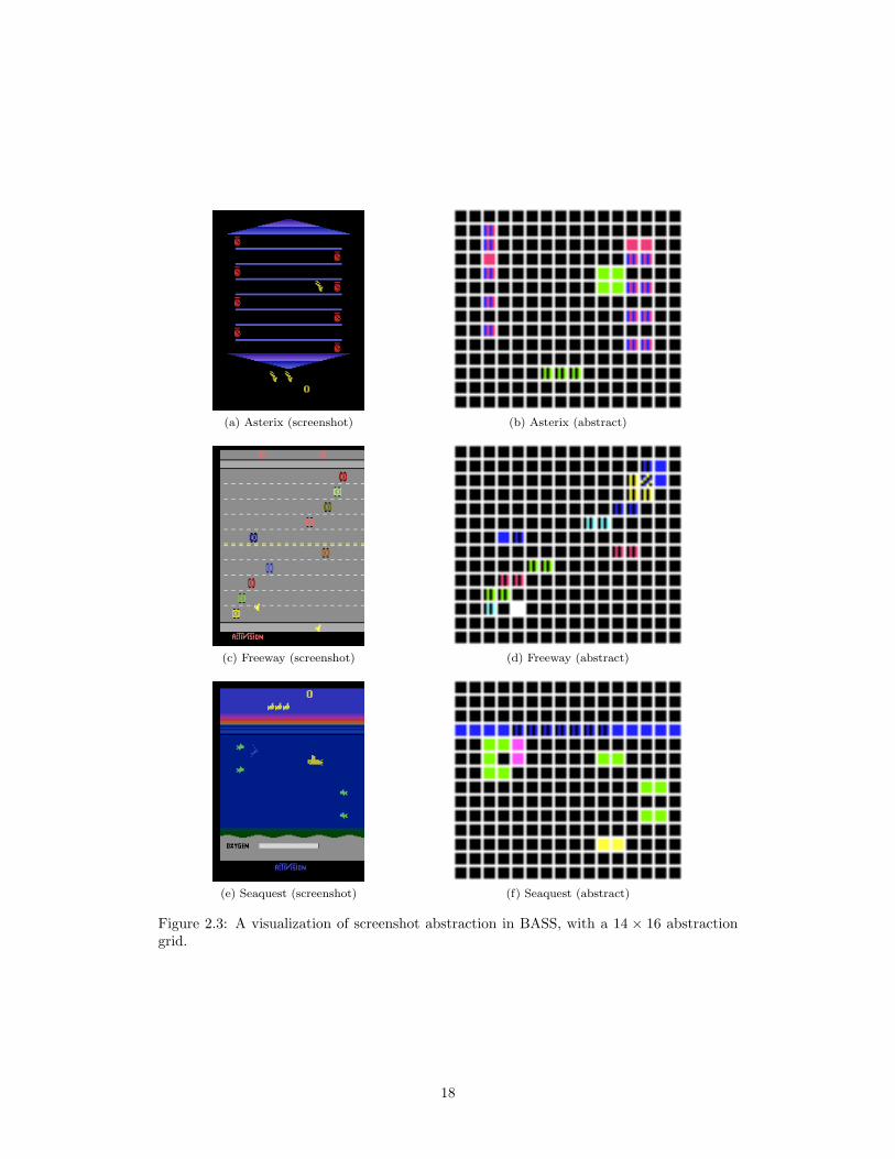
2.3 presents a visualization of how the screenshots from three of the training games compare

with their corresponding abstracted version. Each cell in the grid represents the SECAM

colors present in that sub block. A black cell indicates that all the pixels in this block are

identical to the background. Note that the resulting abstraction is often much more sparse

than the original screenshot.

Aside from the existence of objects in different locations, we are also interested in the

relation between them. For instance, in the case of the game Asterix, it is important to

know if there is a green object (player character) in the centre of the screen and a red object

(collectable object) to the right of it. Linear function approximation is unable to capture

these pair relations on its own, so the relation between objects needs to be represented in

the feature vector. To capture the two-object relations, a new vector vq is generated which

contains all the pairwise AND’s of the items in Vl. The vector vq represents the existence

of pairs of objects of different colors in various parts of the screen. For instance, vq(1) = 1

signifies that vl(1) = 1 and vl(2) = 1, which in turn means that there is an object with color

index 1 and an object with color index 2 in the upper left corner of the screen.

For each action a ∈ A, the corresponding feature vector Φa is a (|vl|+|vq|)×|A| bit binary

vector, which contains the concatenated vectors vl and vq in the location corresponding to

action a, and 0’s everywhere else.

Figure 2.4 shows the pseudocode for the BASS feature vector generation method. Note

that this pseudocode generates the full feature vector Φ. In practice, this vector will be very

sparse, and we will only store the one-indices I(Φ). The BASS-Agent is based on combining

the linear gradient-descent Sarsa(λ) algorithm (Figure 2.1) with the BASS feature vector

generation method.

17

(a) Asterix (screenshot) (b) Asterix (abstract)

(c) Freeway (screenshot) (d) Freeway (abstract)

(e) Seaquest (screenshot) (f) Seaquest (abstract)

Figure 2.3: A visualization of screenshot abstraction in BASS, with a 14 × 16 abstractiongrid.

18

Assume h,w (height and width of the screen), S (background matrix), σ (mapping fromNTSC to SECAM palette), and m,n (height and width of the grid for screen abstraction)are defined.

generate feature vector(screen matrix X):

1. Generate a mapped matrix X with background removed:

for y = 1 to h:

for x = 1 to w:

X(y, x) =

σ(X(y, x)) If X(y, x) 6= S(y, x)−1 Otherwise

2. Divide X into a grid of m× n blocks Bi∈{1,...,m},j∈{1,...,n}3. For each sub block Bi,j generate an 8-bit vector vBi,j . Concatenate these vectors to

produce vl:

vl = []For i = 1 to m, j = 1 to n:

For c = 1 to 8:

vBi,j (c) =

1 If color c exists in the block Bi,j0 Otherwise

vl = concatenate(vl, vBi,j )

4. Generate vq by pairwise AND’ing the items of vl:

vq((i− 1)|vl|+ j) = AND(vl(i), vl(j)) ∀i ∈ {1, ..., |vl|}, j ∈ {i, ..., |vl|}

5. Generate the final feature vector Φ from vl and vq:

v = concatenate(vl, vq)k = |v|

for a ∈ A a, Φa(i) =

v(i+ ak) ak ≤ i ≤ (a+ 1)k0 Otherwise

6. Return Φ

aHere we assume that each discrete action a ∈ A is assigned an integer value between 0 and |A| − 1.

Figure 2.4: Feature Vector Generation based on Basic Abstraction of the ScreenShots(BASS)

19

(a) (b)

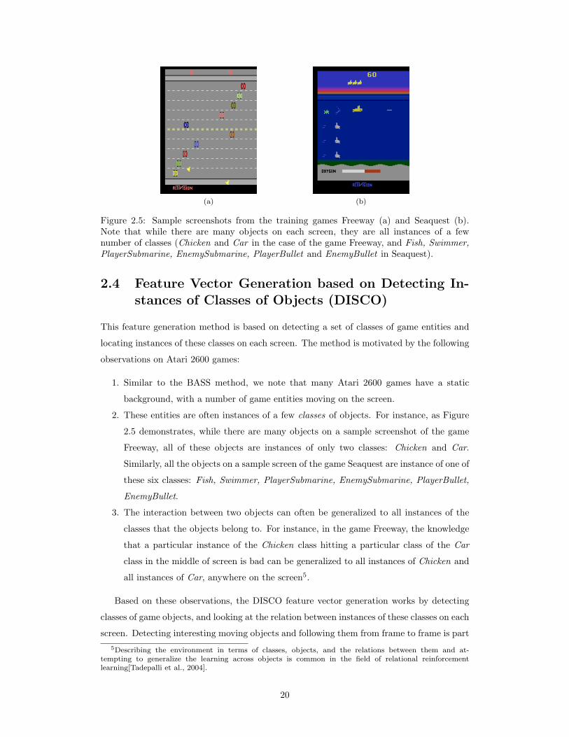
Figure 2.5: Sample screenshots from the training games Freeway (a) and Seaquest (b).Note that while there are many objects on each screen, they are all instances of a fewnumber of classes (Chicken and Car in the case of the game Freeway, and Fish, Swimmer,PlayerSubmarine, EnemySubmarine, PlayerBullet and EnemyBullet in Seaquest).

2.4 Feature Vector Generation based on Detecting In-stances of Classes of Objects (DISCO)

This feature generation method is based on detecting a set of classes of game entities and

locating instances of these classes on each screen. The method is motivated by the following

observations on Atari 2600 games:

1. Similar to the BASS method, we note that many Atari 2600 games have a static

background, with a number of game entities moving on the screen.

2. These entities are often instances of a few classes of objects. For instance, as Figure

2.5 demonstrates, while there are many objects on a sample screenshot of the game

Freeway, all of these objects are instances of only two classes: Chicken and Car.

Similarly, all the objects on a sample screen of the game Seaquest are instance of one of

these six classes: Fish, Swimmer, PlayerSubmarine, EnemySubmarine, PlayerBullet,

EnemyBullet.

3. The interaction between two objects can often be generalized to all instances of the

classes that the objects belong to. For instance, in the game Freeway, the knowledge

that a particular instance of the Chicken class hitting a particular class of the Car

class in the middle of screen is bad can be generalized to all instances of Chicken and

all instances of Car, anywhere on the screen5.

Based on these observations, the DISCO feature vector generation works by detecting

classes of game objects, and looking at the relation between instances of these classes on each

screen. Detecting interesting moving objects and following them from frame to frame is part5Describing the environment in terms of classes, objects, and the relations between them and at-

tempting to generalize the learning across objects is common in the field of relational reinforcementlearning[Tadepalli et al., 2004].

20

of an important field in computer vision, called tracking. There are numerous deterministic

and probabilistic approaches proposed to solve this problem in the tracking literature6. For

the purpose of this research, we are using very simple methods to deal with the tracking

problem7. This is done in the following steps:

• Before the RL-agent starts acting in the game (pre-computation):

– Background detection: The static background matrix S is detected from a set

of game screens. In our experiments, the sample game screens are generated by

acting randomly in each game8.

– Blob extraction: the static background is subtracted and a list of moving blob

objects is detected from each game screen.

– Class discovery: a set of classes of objects C is detected from the extracted

blob objects.

• While the RL-agent is acting in the game:

– Class instance detection: Once the RL-agent starts acting, on each time step,

instances of classes c ∈ C are detected from the current screen matrix.

– Feature vector generation: A feature vector is then generated from these

detected instances.

The following sections explain each of the five steps in details.

2.4.1 Background Detection

A histogram-based method is used to detect the static game background. Given a set of

sample screenshots, a histogram is generated for every pixel on the screen, counting the

colors that appear in that pixel. The background color for a pixel is then set to the most

frequent color in that pixel. Figure 2.6 contains the pseudocode for this method.

Although simple, this method often works well in games with a static background. This

is because it does not need to deal with noise or a moving camera, two of the main challenges

in background detection tasks9.

2.4.2 Blob Extraction

The goal of blob extraction is to find connected regions from the screen matrix, after the

static background is removed. This is done in two steps. First, a sequential labeling algo-6See [Yilmaz et al., 2006] and [Forsyth and Ponce, 2002] for overviews on the current tracking methods

employed in the computer vision community7We note that employing more advanced computer vision techniques can potentially improve the current

results.8They could also be generated by having one of the search-based or RAM-based agents play the game.9This is only true when the assumption of a static background holds. For games with a moving back-

ground, this method will not perform very well and a more advanced background detection method isrequired.

21

Assume h,w (height and width of the screen) is defined.

detect background(screen matrix [X1, X2, ..., Xn])

1. Initialize a histogram for each pixel on the screen:

for i = 1 to h:

for j = 1 to w:

hij = ~0

2. Go through the screenshots and fill in the histograms:

for f = 1 to n:

for i = 1 to h, j = 1 to w:

hij(Xf (i, j)) = hij(Xf (i, j)) + 1

3. For each pixel, pick the most frequent color as the background color:

for i = 1 to h:

for j = 1 to w:

S(i, j) = arg maxc

(hij(c))

4. Return S

Figure 2.6: Pseudocode for histogram-based background detection

rithm [Horn, 1986] marks 8-connected regions which share the same color. These regions are

then compared with the regions labeled on the previous frame, and the neighboring blobs

that are moving with the same velocity are merged together. The merging step allows us

to detect blob objects of different colors, or objects with small gaps between their subparts.

Figure 2.7 contains the pseudocode for our blob extraction method. Figure 2.8 shows the

original game screen, the static background detected, the initial labeled regions, and the

final merged blobs for the games Freeway and Seaquest.

2.4.3 Class Discovery

A class of objects is a collection of all shapes that represent an entity in a game. Often, these

shapes represent different animation frames of an entity. They can also represent obscured

or clipped versions of other shapes in this class.

Our general approach to discovering classes of objects is to look at a sequence of game

screens [X1, X2, ..., Xn], and for each object ot on screen Xt, try to find the object o′t−1 that

represents the same entity in the previous frame Xt−1. If o′t−1 is found and it is different

from ot, we can conclude that the two shapes belong to the same class.

To find the object that represents the same entity in the previous frame, we assume that

any two sequential animation shapes o′t−1 and ot have the following properties:

1. distance(o′t−1, ot) < d. That is, the two objects are relatively close to each other. This

is because objects cannot move arbitrary fast on the screen or the player would not

22

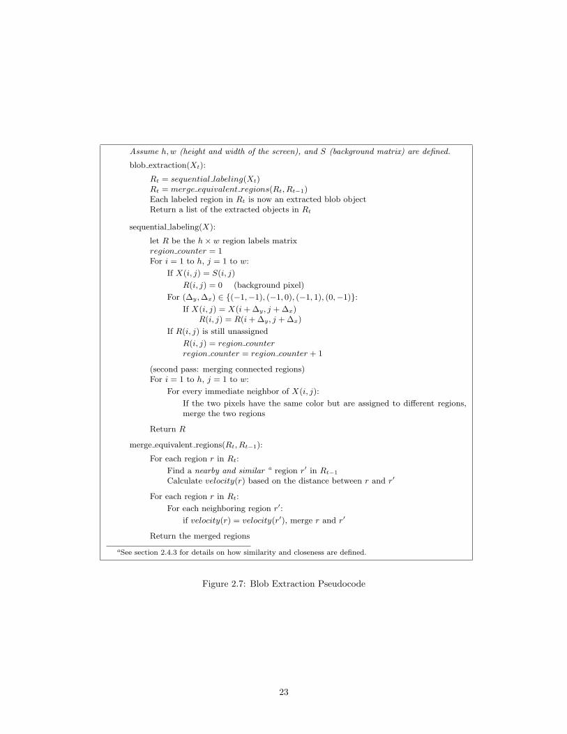
Assume h,w (height and width of the screen), and S (background matrix) are defined.

blob extraction(Xt):

Rt = sequential labeling(Xt)Rt = merge equivalent regions(Rt, Rt−1)Each labeled region in Rt is now an extracted blob objectReturn a list of the extracted objects in Rt

sequential labeling(X):

let R be the h× w region labels matrixregion counter = 1For i = 1 to h, j = 1 to w:

If X(i, j) = S(i, j)

R(i, j) = 0 (background pixel)

For (∆y,∆x) ∈ {(−1,−1), (−1, 0), (−1, 1), (0,−1)}:If X(i, j) = X(i+ ∆y, j + ∆x)

R(i, j) = R(i+ ∆y, j + ∆x)

If R(i, j) is still unassigned

R(i, j) = region counterregion counter = region counter + 1

(second pass: merging connected regions)For i = 1 to h, j = 1 to w:

For every immediate neighbor of X(i, j):

If the two pixels have the same color but are assigned to different regions,merge the two regions

Return R

merge equivalent regions(Rt, Rt−1):

For each region r in Rt:

Find a nearby and similar a region r′ in Rt−1

Calculate velocity(r) based on the distance between r and r′

For each region r in Rt:

For each neighboring region r′:

if velocity(r) = velocity(r′), merge r and r′

Return the merged regions

aSee section 2.4.3 for details on how similarity and closeness are defined.

Figure 2.7: Blob Extraction Pseudocode

23

(a) Original Screenshot (b) Detected Background (c) Extracted Blobs (Pre-Merge)

(d) Extracted Blobs(Post-Merge)

(e) Original Screenshot (f) Detected Background (g) Extracted Blobs (Pre-Merge)

(h) Extracted Blobs(Post-Merge)

Figure 2.8: Background Detection and Blob Extraction for the games Freeway (a-d) andSeaquest (e-h). In the Extracted blob panels, each color indicates a distinctly labeled region.

be able to see them.

2. shape similarity(o′t−1, ot) > s. That is, the two objects are relatively similar to each

other. Generally, if the animation shapes change drastically from frame to frame, the

game will look jumpy and hard to follow10.

To find o′t−1 corresponding to ot, we look at all the objects in Xt−1 which are within d-pixel

neighborhood of ot. Among these objects, if the object that is the most similar to ot passes

the shape similarity(o′t−1, ot) > s test, it will be assigned as o′t−1. Figure 2.9 contains the

pseudocode for our class-dicovery approach. Figure 2.10 shows the discovered classes and

the shapes associated to each class for the game Freeway. Note that the second and the

third classes both represent the Car game entity. Also, the last class, with only one shape,

does not represent any meaningful entity in the game.

There are two main problems with the current method of class discovery. The first

problem is that in addition to the real game entities, the method discovers many junk classes.

These classes often correspond to frequently changing areas in the game background. The

waterline in the game Seaquest (Figure 2.3e) is an example of a local area with frequently

10It is common for Atari 2600 games to have shapes that change considerably in color from frame toframe. Therefore, when looking at objects similarity, we only consider the shapes of the objects and nottheir coloring.

24

Assume d, s (distance and similarity thresholds) are defined.

discover classes([X1, X2, ..., Xn]):

C = []for t = 2 to n:

Ot = blob extraction(Xt)for ot ∈ Ot:

if ot is already in any class c ∈ Cot.class = ccontinue

o′t−1 = find prev obj(ot)if o′t−1 exists:

c = o′t−1.classot.class = cc.add shape(ot)

else:

Let cnew be a new classcnew.add shape(ot)C.insert(cnew)ot.class = cnew

Return C

Figure 2.9: Class Discovery Pseudocode

Figure 2.10: Discovered classes in the game Freeway. Each horizontal section contains theshapes belonging to a class.

changing background. We attempt to address this issue by filtering out classes that do not

appear on the screen frequently enough or are limited to a very small area on the screen.

A second problem with the current approach is that shapes of a single game entity can be

assigned to multiple classes. For example, if there are two different shapes of a single class

on the very first frame, two separate classes will be created for them. This is particularly

problematic because, as we will discuss in section 2.4.5, the length of the feature vector

grows quadratically with the number of classes. To address this, if the number of discovered

classes is too large for feature vector generation, classes that contain similar objects are

automatically merged together. The merging process is continued until we are left with an

acceptable number of classes.

25

Assume C (discovered classes) and L (list of all shape objects for all classes, sorted by sizefrom larger to smaller) are definedFor each c ∈ C, Ψt(c) will hold the instances of the class c detected on the screen Xt

detect class instances(Xt):

For o ∈ L:

Scan the foreground pixels of Xt for a match to oIf there is a match:

1. Mark the matching pixels of Xt, to prevent a rematch to a smaller shape2. c = o.class3. Let ψnew be a new instance, containing the coordinate of the match4. Ψt(c).add(ψnew)

Return Ψt

calculate instance velocities(Ψt, Ψt−1):

For c ∈ C:

For ψt ∈ Ψt(c):

ψ′t−1 = nearest instance to ψt in Ψt−1(c)ψt.velocity = distance(ψt, ψ

′t−1)

Figure 2.11: Pseudocode code for class instance detection and calculating instance velocities

2.4.4 Class Instance Detection

Class instance detection is the process of finding instances of the previously discovered

classes on a given screen. More precisely, for every class c ∈ C, we want Ψt(c) to contain

the list of the coordinates and velocities of all instances of class c on the screen Xt. To

achieve this, a list of all shape objects of all classes is generated. This list is then sorted by

size, from larger to smaller. For each shape object o in this list, the game screen is scanned

to see if there is a match between the shape object and a set of non-background pixels on

the screen. Once a match is found, the matching pixels on the screen are marked to prevent

a second match to a smaller object. The centroid of the matching pixels is then added to

Ψt(o.class).

To calculate the velocity of each instance ψt ∈ Ψt(c), we find its corresponding instance

ψ′t−1 in the list of instances of class c during the previous frame (Ψt−1(c)). The velocity is

determined based on the distance between ψt and ψ′t−1.

Figure 2.11 contains the pseudocode for class instance detection and calculation of the

instance velocities. Figure 2.12 presents the class instances detected in the games Freeway

and Seaquest.

2.4.5 Feature Vector Generation

Once we are able to detect instances of the discovered classes on the current screen, the

next step is to generate a feature vector based on these instances. We would like the feature

vector to capture the following concepts:

26

(a) (b)

Figure 2.12: Class instances detected in sample screens of Freeway and Seaquest. Eachcolored square represents an instance of a discovered class. The small white lines indicatethe calculated object velocities.

• Presence of at least one instance of each class. In many games the knowledge that a

particular entity is on the screen or not is a big indication of how the agent should

act.

• The absolute position of each instance. For example, in the game Freeway, the y-value

of the PC character is highly predictive of the expected future reward.

• The relative position and velocity of every pair of instances. This will allow the agent

to learn and generalize over the interaction of game entities.

A discovered class can have from zero to hundreds of instances on a given screen. This

results in a problem of how to generate a fixed-length feature vector from a varying number

of instances. We will first discuss the feature vector generation method in a toy example

where each class has exactly one instance on the screen. Once the simple case is clear, we

will introduce our method for handling multiple instances of each class.

Imagine a fictional version of the game Freeway, in which at any time step t, we have

exactly one instance of the Chicken class ψckn and exactly one instance of the Car class ψcar.

Figure 2.13 demonstrates how a feature vector can be generated from these two instances.

The first part of the feature vector contains the tile-coding of the absolute position of ψckn.

Similarly, the second part contains the tile-coding of the absolute position of ψcar. The

final part contains the tile-coding of the relative position and relative velocity of the two

instances:

Φ = concat

0BB@TC „ ψckn.xψckn.y

«, TC

„ψcar.xψcar.y

«, TC

0BB@ψckn.x− ψcar.xψckn.y − ψcar.y

ψckn.velx − ψcar.velxψckn.vely − ψcar.vely

1CCA1CCA

27

Figure 2.13: An illustration of the feature vector generated for the game Freeway, in thesimple case where there exists exactly one instance of each class. The feature vector consistsof three sections. Each section contains a binary sub-vector generated by tile-coding thedisplayed variables.

The next step is to expand this method to the more realistic case, in which multiple

instances of a class can exist on the screen. To generate a fixed-length feature vector, we

note that while the number of instances of each class is variable, the overall number of

discovered classes is constant. Consequently, a sub-section of the feature vector is reserved

for each discovered class, as well as each pair of classes. When we have multiple instances

of a class c1, a sub-vector is generated for each instance. The sub-vectors are then added

together and placed in the section of the feature vector reserved for class c1:

Φ[c1] =∑

ψi∈Ψ(c1)

TC

(ψi.xψi.y

)

where Φ[c1] is the section of the feature vector reserved for the class c1. Similarly, all possible

pairings of the instances of two class c1 and c2 are added together, and populate the section

reserved for the pairing of the two classes:

Φ[c1, c2] =∑

ψi∈Ψ(c1),ψj∈Ψ(c2)

TC

ψi.x− ψj .xψi.y − ψj .y

ψi.velx − ψj .velxψi.vely − ψj .vely

Figure 2.14 illustrates this approach for an imaginary screen of the game Freeway, with

one instance of the class Chicken and two instances of the class Car. With two discovered

classes, the final feature vector will have three sections: one reserved for the absolute position

of the Chicken class, one reserved for the absolute position of the Car class, and one reserved

for the relative position and velocity of (Chicken, Car) pair. Since we only have one instance

of the class Chicken, the position of this one instance is tile-coded and placed in the first

section of the feature vector. With two instances of class Car, each instance is tile-coded

individually and the resulting vectors are added together and placed in the second section of

the feature vector. Similarly, the pairs of the one instance of Chicken and each instance of

28

Figure 2.14: Conceptual figure of feature vector generation for the game Freeway, where wehave one instance of class Chicken and two instances of the class Car.

Car are tile-coded individually, added together, and placed in the final part of the feature

vector.

Finally, for each class c ∈ C a single bit is reserved on the feature vector to indicate the

case when no instance of the class c is present on the current screen. This will allow the

function approximation method to assign non-zero values to the case when no instance of a

class is present.

Figure 2.15 presents the pseudocode for feature vector generation based on Detecting

Instances of Classes of Objects (DISCO). Note that the presented pseudocode generates a

full feature vector. Similar to the BASS method, in practice we like to store the non-zero

indices only. However, the feature vector generated by DISCO is not a binary vector. To

store values that are larger than one, the indices for these values are represented multiple

times. For instance, a full vector v = [1, 0, 0, 0, 0, 0, 3, 0, 2] can be represented as I(v) =

[0, 6, 6, 6, 8, 8]. This will allow us to use the same gradient-descent Sarsa(λ) algorithm (figure

2.1) on a non-binary feature vector.

2.5 Feature Vector Generation based on Console Mem-ory (RAM)

Unlike the previous two methods, which generate feature vectors based on the game screen,

this method generates a feature vector based on the content of the console memory. The

Atari 2600 has only 128× 8 = 1024 bits of random access memory11. The complete internal

state of a game (including the location and velocity of game entities, timers, and health

indicators) must be stored in these 1024 bits. For a human player, it is close to impossible11Some games include additional RAM on the game cartridge. For instance the Atari Super Chip in-

cluded an additional 128 bytes of memory [Montfort and Bogost, 2009]. However, the current approachonly considers the main memory included in the Atari 2600 console.

29

Assume C (list of discovered classes) is defined.

generate feature vector(screen matrix Xt)

1. Ψt = detect class instances(Xt)2. calculate instance velocities(Ψt,Ψt−1)

3. Generate the absolute position sections of the feature vector

for c ∈ C:

Φ[c] =X

ψi∈Ψt(c)

TC

„ψi.xψi.y

«

4. Generate the relative position/velocity sections of the feature vector

for c1 ∈ C:

for c2 ∈ C:

Φ[c1, c2] =X

ψi∈Ψt(c1),ψj∈Ψt(c2)

TC

0BB@ψi.x− ψj .xψi.y − ψj .y

ψi.velx − ψj .velxψi.vely − ψj .vely

1CCA5. For each class c, reserve one bit at Φ[∅c] that is one when there is no instance of c on

screen:

for c ∈ C:

Φ[∅c] =

1 if |Ψt(c)| = 00 Otherwise

6. Return Φ

Figure 2.15: Feature Vector Generation based on Detecting Instances of Classes of Objects(DISCO)

30

to figure out how to play a given game by only looking at these seemingly random bits. The

purpose of our RAM-based agent is to investigate if an RL-based agent can learn how to

play a given game using feature vectors generated only from the content of the memory.

The first part of the generated feature vector, denoted by vl, simply includes the 1024 bits

of RAM. We note that Atari 2600 game programmers often use these bits not as individual

values, but as part of 4-bit or 8-bit words. Fortunately, doing linear function approximation

on the individual bits can capture the value of the multi-bit words. For instance, assume

that the programmers of the game Freeway store the y-value of the Chicken location in a

4-bit word stored in address 16 to 20. Furthermore, let us assume that the optimal value of

a state is linearly proportional with the y-value of the Chicken in that state, with a constant

of 0.2. Linear function approximation can capture this relation as:

V ∗ = 0.2× 1× vl[19] + 0.2× 2× vl[18] + 0.2× 4× vl[17] + 0.2× 8× vl[16]

We are also interested in the relation between pairs of values in memory. To capture

these relations, a new vector vq is generated which contains all the pairwise AND’s of the

bits in Vl. Note that a linear function on bits of vq can capture multiplication products of

both 4-bit and 8-bit words. This is because the multiplication of two n-bit words a and b

can be expressed as a weighted sum of the pairwise products of their bits:

[an−1a1a0]× [bn−1b1b0] = 20b0a0 + 21b0a1 + ...+ 2n−1b0an−1+21b1a0 + 22b1a1 + ...+ 2nb1an−1+...2n−1bn−1a0 + 2nbn−1a1 + ...+ 22n−2bn−1an−1

Figure 2.16 shows the pseudocode for the memory based feature vector generation

method. Note that this pseudocode generates the full feature vector Φ. In practice, we

will only store the one-indices I(Φ). The RAM-Agent is based on combining the linear

gradient-descent Sarsa(λ) algorithm (figure 2.1) with the feature vector generated by this

method.

2.6 Parameter Search

There are two sets of parameters that need to be set for the reinforcement learning based

agents. The first set of parameters are related to the feature vector generation methods. For

instance, in the class discovery step of the DISCO-Agent (section 2.4.3), two thresholds d

and s determine the closeness and similarity of objects. Similarly, two parameters m,n are

required in the BASS-Agent to define the height and width of the abstraction grid. Feature

generation parameters are set to values that generally seem to work well in the training

games.

The second set of parameters belong to the Sarsa(λ) algorithm. These parameters are: α

(learning rate), ε (exploration/exploitation rate), γ (discount factor), and λ. Additionally, as

31

generate feature vector(ram vector M)

1. vl = M

2. Generate vq by pairwise AND’ing the items of vl:

vq(1024(i− 1) + j) = AND(vl(i), vl(j)) ∀i ∈ {1, ..., 1024}, j ∈ {i, ..., 1024}

3. Generate the final feature vector Φ from vl and vq:

v = concatenate(vl, vq)k = |v|

for a ∈ A, Φa(i) =

v(i+ ak) ak ≤ i ≤ (a+ 1)k0 Otherwise

4. Return Φ

Figure 2.16: Feature Vector Generation based on Console Memory (RAM)

Parameter BASS DISCO RAMα (Learning Rate) 0.1 0.01 0.3λ 0.5 0.5 0.3Optimistic Initialization Yes Yes Yesε (Exploration / Exploitattion Rate) 0.1 0.1 0.1γ (Discount Factor) 0.999 0.999 0.999m (Screen Abstraction Grid Height) 14n (Screen Abstraction Grid Width) 16d (Distance Thresholds for Class Discovery) 0.1Maximum Number of Classes 10

Table 2.1: Sarsa(λ) parameter values used in our experiments. The first three values are setby doing a parameter search on the training games. The other parameters are set to valuesthat seem to generally work well in the same set of games.

discussed in section 2.1.4, with Sarsa(λ) there is an option of doing Optimistic Initialization.

For each RL-agent, the values for α, λ, and wether to do Optimistic Initialization are chosen

by doing a parameter search on the training games12. Table 2.1 contains the final parameter

values for the RL-agents.

2.7 Experimental Results on the Training Games

The performance of each agent is compared against two hand-coded agents. The Random

Agent chooses a random action on every frame. The Best-Action Agent first finds the single

action that results in the highest rewards, and returns that same action on every frame. A

t-test is performed to insure that the comparisons with the Random and Best-Action agents

are statistically significant (p = 0.05). In certain cases, we are interested in comparing the

12The range of parameters searched for α is between 0.00001 and 0.3, and the range for λ is between 0.3and 0.8.

32

Game Average Reward per EpisodeBASS DISCO RAM Best-Action Random Author

Asterix 402† 301† 545† 250 156 1380Freeway 0 0 0 5 0 12.4Seaquest 129† 61† 119† 41 27 1286SpaceInvaders 105† 53 105† 92 59 458

Table 2.2: Results of the three reinforcement learning based agents on the training games.The results specified by † are significantly higher than both the Best-Action and Randomagents results (p = 0.05).

performance of an agent with the performance of a typical human player. In these cases,

we report the score received by the author playing the game for the same amount of time,

averaged over five trials. We note that the numbers reported here are by no means close to

the best performance of an expert player, but rather the performance of a typical human

player with little practice on a given game. The results are averaged over the last 1000

episodes, after 18 × 106 steps of training. Please see sections 4.1 to 4.3 for an overview of

the evaluation method and the details of the experimental setup.

Table 2.2 summarizes the results of the three RL-based agents on the training games.

Figure 2.17 shows the learning progress of the RL-agents on the training games. Except

for the game Freeway, all three agents perform significantly better than both the Random

Agent and the Best-Action agent. However, we note that none of the results are close to

the performance of a typical human player.

2.8 Discussion

This section explores a number of challenges for our Sarsa(λ) agents to match the perfor-

mance of humans, and possible steps that can be taken to overcome them.

2.8.1 Sensitivity to the Learning Rate (α)

While performing parameter search for the RL-agents, we noted that all three agents are

very sensitive to the learning rate parameter α. For each agent/game pairing, there is a

small range of α values in which the agent performs reasonably well, while for other values it

does performs poorly13. Table 2.3 presents the α and λ values for the top five performances

of the RAM-Agent on three of the training games. Note that the RAM-agent performs best

on the game Asterix when α = 0.3 while its best performance on the game Freeway is with

α = 10−5. Furthermore, the rest of the parameter search results show that the RAM-Agent

does not perform very well on Asterix with α = 10−5(average reward = 117) and it performs

very poorly on Freeway with α = 0.3 (average reward = 0).

13The gradient-descent function approximation can even diverge for some larger values of α.

33

(a) Asterix (b) Freeway

(c) Seaquest (d) SpaceInvaders

Figure 2.17: Learning progress for the RL-agents on the training games. Each point on thegraphs is a moving average over 200 episodes. The two horizontal lines indicate the averageperformance level for the Random and BestAction agents.

Asterix Freeway Seaquestreward α λ reward α λ reward α λ

545 3× 10−1 0.3 2.3 1× 10−5 0.5 135 1× 10−1 0.3478 3× 10−1 0.5 2.3 1× 10−5 0.8 127 1× 10−2 0.3452 3× 10−1 0.8 2.2 1× 10−5 0.3 121 1× 10−2 0.5398 1× 10−1 0.3 2.1 1× 10−4 0.8 119 3× 10−1 0.3377 1× 10−1 0.5 2.0 1× 10−4 0.5 115 1× 10−1 0.5

Table 2.3: Sarsa(λ) (with optimistic initialization) parameter values for the top five perfor-mances of the RAM-Agent on three of the training games. Rewards are averaged over 1000episodes.

34

Asterix Freeway Seaquestreward θ λ reward θ λ reward θ λ575.63 1× 10−6 0.5 0.02 5× 10−5 0.8 123.88 1× 10−5 0.5532.33 1× 10−6 0.8 0.02 1× 10−4 0.3 108.51 1× 10−5 0.8531.33 1× 10−6 0.3 0.02 1× 10−5 0.8 104.54 1× 10−5 0.3

Table 2.4: The meta-learning rate (θ) and λ for the top three performances of the RAM-agent with iDBD on three of the training games. Rewards are averaged over 1000 episodes.

The state dynamics, reward signal, and shape of the optimal value function can be com-

pletely different for two distinct games. In a way, playing two different games is comparable

to solving two entirely unrelated problems. Therefore, it is not unexpected that each game

has its own optimal learning rate, and it is difficult to find a common learning rate that

performs well across all games.

The alternative to using a static learning rate is to use a meta-learning method that can

learn α from previous experience. We implemented two meta-learning methods: Delta-bar-

Delta [Jacobs, 1987] and iDBD [Sutton, 1992]. Both methods keep a separate learning rate

for each item in the weights vector Θ. The intuition behind both methods is to look at the

historic changes in the learning rate of each item, and increase it if the previous updates

have similar signs and decrease it if the updates have opposite signs. In other words, when

the updates are in the same direction, we probably are not making large enough changes.

On the other hand, if the updates are in opposite directions, then we are probably making

too big of steps and should decrease the learning rate. Both methods have a number of

meta parameters determining the initial values and the step size for updating the learning

rates.

In our experiments, neither of the meta-learning methods performs noticeably better

than the static α approach. Similar to the static learning rate approach, both Delta-bar-

Delta and iDBD are sensitive to the meta parameters, and each agent/game pair performs

best with a different set of meta parameters. For instance, Table 2.4 presents the meta-

learning rate (θ) and λ for the top five performances of the RAM-agent with iDBD on

three of the training games. Once again, there is a different range of θ values in which the

agent performs well. Atari 2600, with a substantial number of games each having a unique

reward structure and value function, is an excellent platform for developing and testing

meta-learning methods for reinforcement learning.

2.8.2 Delayed Rewards and Delayed Consequences

In an MDP with delayed rewards the agent receives rewards of zero in most of the states,

and only receives a non-zero reward after it has executed a complex sequence of actions

[Conn and Peters, 2007]. Decision problems with delayed rewards are well known to be

35

complicated and hard to solve [Laud and DeJong, 2003]. It is important to note that one of

the main reasons for learning a value function is to address this issue. However, problems

with very sparse rewards are inherently hard problems, which are even challenging for the

human mind. As an example, consider a two-handed bandit with two possible actions:

Left and Right. The bandit always returns a reward of zero, except if the sequence of

{25×Left, 25×Right, 50×Left} is exactly followed, in which case it returns a very large

reward. Without any prior knowledge on the bandit, finding an optimal policy (or even

a policy the performs relatively well) is an extremely difficult problem, even for a human

agent.

Since the game score is the only reward signal used, many Atari 2600 games end up with

very delayed rewards. This is because games often do not give intermediate scores. That is,

the player only receives a score once she has finished accomplishing the required task. For

instance, in the game Freeway the agent will receive rewards of zero in every state until the

Chicken finishes crossing the street. At this point, the agent will receive a non-zero reward

in one state and then will continue receiving zero rewards again.

In addition to delayed rewards, some Atari 2600 games involve other delayed conse-

quences that further complicate the learning task. For instance, there is a relatively long

delay (over 100 frames) in both games Seaquest and Space-Invaders between the time that

the player character dies and the time when the player-agent is informed of this death.

Furthermore, as in the case of the game Asterix, a death animation may be shown to the

player which changes the game screen considerably during this delay. The death delay and

animation can lead the learning algorithm to blame the wrong features for the death of the

PC, which further complicates the learning task.

A parallel to the delayed rewards, and another challenging situation, is when a game

provides only a narrow path to survival and most action sequences lead to a game-over. For

instance, in the game Seaquest, when the player character is at the bottom of the screen and

the oxygen tank is near empty, the player needs to immediately come to the surface (that

is, perform an action sequence similar to [up, up, ..., up]) or the game will be over. This is

challenging to learn, since the ε-greedy exploration is unlikely to produce the correct action

sequence.

2.8.3 Complex Value Function

Many Atari 2600 games have optimal value functions that are far more complex than what

the linear combination of the current generated features can estimate. The assumption

behind using linear function approximation is that the presence or absence of each feature

only has an additive effect on the value function. This assumption does not always hold in

Atari 2600 games. Consider the following two stages in the game Seaquest:

36

Figure 2.18: Screenshot from the game SpaceInvaders demonstrating the Non-Markovianproperty of an Atari 2600 game screen. Note that from this screenshot alone one cannottell if the bullet (the vertical white line) is moving upward or downward.

1. Before rescuing five swimmers, the player needs to rescue swimmers while shooting at

fishes and other submarines. At this point, going to the surface should be avoided,

since the player will lose a swimmer.

2. After rescuing five swimmers, the player needs to immediately go to the surface and

receive a large score. Rescuing more swimmers has no effect at this point.

The optimal policy for the game dramatically changes with a small variation on the screen

(appearance of the fifth rescued swimmer at the bottom of the page). States that were

previously estimated to have a high value (states associated with rescuing a swimmer)

suddenly have a low value. On the other hand, some low value states (states with the player

character on the surface) suddenly have a high value. Linear function approximation on any

of our current feature generation methods is unable to capture this complexity in the value

function. To address this, one can either use a non-linear function approximation method

(e.g., neural networks) or generate more complex feature vectors.

2.8.4 Non-Markovian States

As discussed in section 2.1.1, the states of an MDP are assumed to have the Markov property.

That is, each state should summarize all relevant information from the past interactions.

However, the Markov assumption often breaks when generating a feature vector from the

current game screen. Figure C.1 illustrates how the Markov assumption breaks in a screen-

shot of the game SpaceInvaders. Note that this screenshot does not summarize all relevant

information from the past history. Particularly, from this screenshot alone one cannot tell

if the bullet (the vertical white line) is moving upward or downward. This is important

information, since not knowing the direction of the bullet prevents us from determining if

we are in a good state, i.e., the PC has just shot a bullet at the Aliens, or in a bad state,

i.e., the PC is about to be hit by a bullet from the Aliens.

37

A possible way to address this problem is to include the screenshot or the content of

memory from the previous time step. For instance, in the BASS method, we can generate

an abstract version of both the current scree and the previous screen, and then look at pairs

of items in both screens. Finally, note that the DISCO-agent already addresses this problem

to some extent, since it looks at the previous screen to determine the velocity of each game

entity. Also, the content of RAM must be Markovian, since it contains the full state of the

game.

2.8.5 Challenge of Playing Arbitrary Games

We can summarize almost all of these challenges as the single challenge of trying to learn to

play arbitrary games. When solving a specific problem, we are able to include our knowledge

about the problem into the feature generation, reward signal, weights initialization, episode

length, and other properties of the experiment. This is not the case when designing an

algorithm to learn arbitrary problems.

The challenges listed in the previous sections can often be easily addressed when solving a

single game. A suitable learning rate can be found using parameter search. Delayed rewards

and consequences can be overcome using various reward shaping [Randløv and Alstrøm, 1998]

techniques. Complex value functions can be simplified by customizing the feature vector

and manually including important non-linear feature pairings. For instance, in the case

of the complex value function for the game Seaquest (discussed in section 2.8.3), one can

generate a customized feature vector by pairing the existence of the fifth rescued swimmer

at the bottom of the screen with every other feature. The resulting vector is twice the size

of the original vector, and is able to capture the dramatical changes of the value function

with linear approximation.

To illustrate this point, a customized agent is implemented for Freeway, the game in

which our current generic agents have the poorest performance. A game-specific feature

vector is generated by tile-coding the y-coordinate of the Chicken with the x-position of

each of the Cars. The agent receives a reward of -1 on each time step, except when it

completely crosses the screen, in which it gets a reward of zero and the episode ends. We

also experimented with a number of learning rates to find the most suitable α value for

this game. After only 18000 time steps (0.1% of the usual training period) the Sarsa(λ)

converged to a very good policy, generating an average of 13.5 scores per each minute of

game play. This performance is even significantly better than the performance of the author

playing this game.

38

Chapter 3

Search-based Methods

This chapter explains how a state-action tree can be generated for any Atari 2600 game by

using the emulator to simulate the consequence of various actions in the future. General

search methods can then be applied the generated tree to play a given game. Unlike the

reinforcement learning methods discussed previously, there is no learning involved in the

methods discussed here. Instead, the challenge is how to use a limited number of simulation

steps in order to best play an Atari 2600 game.

Initially, it may appear that allowing the agent to peek into the future and see the

consequence of its actions reduces playing Atari 2600 games to a trivial problem. However,

the massive state-space of Atari games and the limited number of simulation steps that

are allocated to the agent per each frame, make this problem far from trivial. As an

example, consider a game with only 4 actions. At 60 frames per second, to look ahead

only one minute into the game, the agent needs to simulate 460∗60 ≈ 102160 frames. This is

clearly infeasible. Fortunately, the AI community has developed a rich arsenal of smarter

strategies for exploring and pruning the state-action tree. These methods will allow us to act

intelligently in the game, while only simulating a very small fraction of the full state-space.

3.1 Generating a State-Action Tree

The save-state and restore-state features of the emulator are used to generate a state-action

tree. When issued a save-state command, the emulator saves all the relevant data about

the current game, including the contents of the RAM, registers, and address counters, into

a variable. Similarly, the restore-state command restores the state of the current game from

a previously saved state.

Figure 3.1 demonstrates how the save-state/restore-state features can be used to generate

a state-action tree. Originally, the agent is at some point in the middle of the game Seaquest

(3.1a). Using save-state, the state of this node is stored into s0, the root of the tree (3.1b).

Next, we simulate taking the Left action for 15 frames (3.1c), and save the resulting state

39

into state s0,L(3.1d). We then restore the original state s0 (3.1e), and simulate taking the

Right action for 15 frames (3.1g). The resulting state is saved into state s0,R (3.1h). In this

fashion, we can expand the full state-action tree.

Each node s in the tree contains:

• The state variable generated by the save-state command

• r(s):the reward received during the simulation node s

• V (s): cumulated discounted1 reward of the sub-branch starting from s

• C(s): set of child nodes of s

Note that since there is no natural ending for many Atari 2600 games, we need to impose

an arbitrary limit on the expansion of the tree. In our approaches, we define a maximum

number of simulation steps allowed per frame, denoted by M , and use it to limit the tree

expansion.

3.2 A Generic Search-based Agent

Figure 3.2 contains a simple overview of how a generic search-based agent can use the state-

action tree to act in a game. When k = 1, the agent will choose a distinct action on every

frame. However, since a human player cannot generate 60 distinct actions per second on

a joystick, Atari 2600 games are often designed to require a much lower action frequency.

In our experiments, we observe that the agent can act reasonably well in many games with

k in the range of 10 to 20 (that is, 3 to 6 distinct actions per second). There is a tradeoff

involved in setting the value of k: a smaller k value allows finer player action, since the

agent can choose more distinct actions per second. On the other hand, a higher k value

enables us to look further ahead into the game, and get a better estimate of the consequence

of each action.

The function generate tree expands the state-action tree starting from the state s0 and

limiting the tree expansion to kM simulation steps. It returns the action a at the root

which corresponds to the sub-branch with the highest discounted sum of rewards. Any tree

search algorithm can be used for the tree expansion. The following two sections demonstrate

how generate tree can be implemented using breadth-first search (Section 3.3) and UCT

(Section 3.4).

3.3 Full-Tree Search

A simple method to use for the search-based agent is to fully expand the tree breadth-first,

until the maximum number of simulation steps is reached. Once the tree is fully expanded,1Discounting the future values insures that the agent will go after rewards that are closer first.

40

(a) Original state (b) S0 set as root of the tree

(c) Sim. Left for 15 frames (d) Save-state the new state

(e) Restore-stae S0 (f)

(g) Sim. Right for 15 frames (h) Save-state the new state

Figure 3.1: Illustration of how the state-action tree is built from some initial state S0 forthe game Seaquest, using the save-state/restore-state features of the emulator

41

Every k frame:

1. Save the current state of the game to s0

2. a = generate tree(s0)3. Restore the state of the game back to s0

4. Repeat action a for k frames

Figure 3.2: A generic search-based agent

the node values are updated recursively from the bottom of the tree to the top:

V (s) = r(s) + γ maxc∈C(s)

V (c) (3.1)

where γ is the discount factor.

3.3.1 Avoiding Death: A Simple Heuristic

“In any case avoid death, since our ancestors disapproved of it.” -Obeyd Zakani,

14th century poet and satirist

In many arcade-style games, if a player can simply keep the Player Character (PC) alive,

it always has the chance to collect more rewards later on in the game. This observation

leads us to a simple heuristic which prunes the sub-branches of the tree that we know will

end up with the death of the PC. More precisely, let d(s) be 1 if we know that the branch

starting from node s will certainly end up with the death of the PC. For a leaf node, d(s)

is 1 if the PC is dead in the state s. For a non-leaf node, we have:

d(s) =∏

c∈C(s)

d(c) (3.2)

That is, a node is declared dead if all of its child nodes are also dead. When we update the

value of a living node, we only consider the values of its children that are also not dead:

V (s) = r(s) + γ maxc∈C(s),d(c)=d(s)

V (c) (3.3)

Once the tree expansion is complete, the search-based agent chooses a sub-branch of the

root with the highest value, which is also not dead. If all sub-branches at the root level are

dead, i.e., if the player will certainly die no matter what action it chooses, the agent will

choose the sub-branch with the highest value.

Figure 3.3 shows the pseudo code for the full-tree search, doing a breadth-first search on

the non-dead states.

3.3.2 Choosing Parameters

As discussed in 3.1, the maximum number of simulation steps allowed per frame (M), is

an arbitrary limit imposed to bound the tree expansion. Ideally, a meaningful limit such as

42

(Assume k,M, γ, available actions are defined)

function generate tree (node s0)

num simulations = 0queue qq.push(s0)while (num simulations < kM and not empty(queue))

s = q.pop()for each a in available actions

sa, r(sa), d(sa)=simulate game(start=s,steps=k,act=a)C(s).insert(sa)num simulations = num simulations+ kif d(sa) = 0

q.push(sa)

update values(s0)a = arg max

c∈C(s0),d(c)=d(s0)V (c)

return a

function update values(node s)

for c in C(s):

update values(c)

d(s) =∏c∈C(s) d(c)

V (s) = r(s) + γmaxc∈C(s),d(c)=d(s) V (c)

Figure 3.3: Full-tree search with the avoiding death heuristic.

43

Game Average Reward per EpisodeFull-Tree Search Best-Action Random Author

Asterix 1980† 250 156 1380Freeway 2.7 5 0 12.4Seaquest 161† 41 27 1286SpaceInvaders 417† 92 59 458

Table 3.1: Results of the full-tree search-agent on training games, compared to the Best-Action and Random agents. Rewards are averaged over 100 episodes. Results specified by† are significantly higher than both Best-Action and Random agents results (p = 0.05).

“the highest M value that permits a real-time run” would be desirable. Unfortunately, none

of the search-based agents are able to run in real-time under the current implementation. In

choosing a value for M , we have attempted to find a value that results in a reasonably good

performance and one that could (with some enhancements to the code) allow a real-time

run. In our experiments, we are using a maximum of 4000 simulation steps per frame, which

currently runs at a frame rate of about two frames per second. Improving the implementa-

tion of the save-state/restore-state features of emulator and simulating disjoint branches in

parallel processes could allow the search-based agents to run in real-time with this limit.

The value of k is set to 20 frames (3 distinct actions per second) by running a parameter

search on the training games. γ is set to 0.99.

3.3.3 Results for the Training Games

Table 3.1 summarizes the results of the Full-Tree Search Agent on the training games, with

M = 4000, k = 20, and γ = 0.99. Please see sections 4.1 to 4.3 for an overview of the

evaluation method and the details of the experimental setup.

In the case of the game Asterix, in which scores are abundant and easily reached, and

both the scores and death are immediately revealed to the player, the full-tree search per-

forms very well. However, the agent is not performing very well in any of the other three

games. In the case of both Space-Invaders and Seaquest, the poor performance is due to

a delay of over 100 frames between the moment that the PC is dead and the time when

the player-agent is informed of this death. This delay makes the full-tree agent unable to

predict and avoid death in either game. In the case of the game Freeway, while the PC never

dies, the reward signal is very sparse. The player only receives a reward when the PC has

completed passing the highway. At the beginning of the game, this reward signal is outside

the reach of the full-tree search, and thus the agent acts randomly. The random move con-

tinues until the PC moves up enough in the highway so that the reward is reachable by the

tree expansion, at which point the search-agent starts acting optimally, and immediately

reaches the top of the highway.

Expanding the full state-action tree limits the agent to a very short window into the

44

future. For instance, in a game with 10 actions, with k = 20 and M = 4000, the agent can

look ahead for 80 to 100 frames, or less than two seconds. Therefore, when the consequences

of the actions are immediate, in other words, when both the reward and death can be

detected within a small window, the full-tree search agent performs well. This explains the

good results obtained in the game Asterix. On the other hand, when the game has delayed

consequences, i.e., when either the reward or detecting and avoiding death falls outside of

this short window, full-tree search performs poorly.

3.4 UCT: Upper Confidence Bounds applied to Trees

As we discussed in the previous section, spending the simulation steps to fully expand

the state-action tree results in a short look-ahead trajectory, which in turn results in poor

performance in games with delayed consequences. A preferable alternative is to simulate

deeper into the more promising sub-branches of the tree. To do this, we need to find a

balance between expanding the higher valued branches and spending simulation steps on

the lower valued branches to get a better estimate of their values. This is an instance of the

well-known exploitation-exploration problem. Additionally, we can apply a t-step random

simulation at the end of each leaf node to get an estimate of a longer future trajectory. These

are the two key ideas in the UCT algorithm. The UCT algorithm, developed by Kocsis and

Szepesvari [Kocsis and Szepesvari, 2006], can potentially allow the agent to simulate deeper

into the more promising branches while addressing the exploration-exploitation problem and

provide us with a method for a t-step random trajectory at the end of each leaf node.

3.4.1 Overview of the Algorithm

Instead of the breadth-first full expansion of the state-action tree, UCT iteratively adds

single leaf nodes to the tree. During each iteration, the algorithm starts at the root of the

tree and recursively chooses sub-branches until it reaches a leaf node. At a leaf node, the

algorithm runs a t-step random simulation, and propagates the received rewards up the tree.

Once all the siblings of a leaf node have received at least one visit, the search will expand

the leaf node and add its child nodes to the tree.

Consider the problem of choosing a sub-branch c ∈ C(s) to visit next during a UCT

iteration. We may already have visited a number of child nodes of s before and have an

estimate of their values. On one hand, it is desirable to visit the child with the highest value,

since we are looking for a deeper expansion in the more promising sub-branches. On the

other hand, we may have a poor estimate of the values of the other sub-branches. Therefore,

we may want to choose a child node with a lower value, in order to improve our estimate

of its value. UCT deals with this dilemma by treating it as a multi-armed bandit problem,

and using a variation of UCB1, which is a “bandit algorithm”, to choose which child node

45

to visit next. In particular, UCT chooses a child node c ∈ C(s) that maximizes:

V (c) + C

√lnn(s)n(c)

(3.4)

where n(s) is the number of times node s has been visited, and C is a constant. The term

C√

lnn(s)n(c) is called the UCT bias. It insures that with the appropriate value of C, the

algorithm is consistent, i.e., “the probability of selecting the optimal action can be made to

converge to 1 as the number of samples grows to infinity” [Kocsis and Szepesvari, 2006].

Figure 3.4 contains the pseudocode for UCT. Figure 3.5 presents a conceptual graph of

how UCT expands the state-action tree. Note that the tree is explored much deeper in some

branches compared to others.

3.4.2 Setting the UCT Bias Constant

According to Kocsis and Szepesvari, for the theoretical guarantees of UCT to hold, the

following two inequalities need to be satisfied with an appropriate value of the bias constant

C [Kocsis and Szepesvari, 2006]:

P

(V (c) ≥ V ∗(c) + C

√lnn(s)n(c)

)≤ n(s)−4

P

(V (c) ≤ V ∗(c)− C

√lnn(s)n(c)

)≤ n(s)−4

where s is any node in the tree, V (c) is the estimated value of one of its child nodes c after

n(c) visits, and V ∗(c) is the true value of the child node.

In applications where the mean and variance of the reward is known, the constant C

can be set beforehand. However, in the case of Atari 2600 games, the reward frequency and

values change considerably both among different games and within various stages of the same

game. Dealing with a similar issue in solving Real-time Strategy games with UCT, Balla

and Fern suggests setting the bias constant to the same value as V (c) [Balla and Fern, 2009].

This insures that the exploration bias and the action values are at least within the same

order of magnitude2. Unfortunately, as Bella suggests, this choice has unknown theoretical

implications.

Our approach to ensure that the action values and the exploration bias are within the

same order of magnitude is to scale the action values down to [−1, 1]. This is done in two

stages. First, all rewards are scaled down3 to [−1, 1]. Furthermore, rewards are also divided

2In our discussions with Nathan Sturtevant, he reports that a number of teams in the General GamePlaying competition [Genesereth and Love, 2005] are also employing a similar tactic. However, to the bestof our knowledge, this has not been documented in any publications.

3We are currently doing this in a naive way: all positive rewards are set to 1 and all negative rewardsset to -1. It might be possible to keep track of the highest and lowest rewards received so far, and do thisscaling in a more intelligent way.

46

(Assume k,M, t, γ, C, available actions are defined)

function generate tree (node s0)

num simulations = 0while num simulations < kM

s = s0

while s is not leaf

if c ∈ C(s) exists with n(c) = 0s = c

else

s = arg maxc∈C(s)

(V (c) + C

√lnn(s)n(c)

)If all siblings of s have been visited at least once

for each a in available actions

sa, r(sa), d(sa)=simulate game(start=s,steps=k,act=a)n(sa) = 0sum reward(sa) = 0C(s).insert(sa)num simulations = num simulations+ k

rmc = do random simulation(start = s, steps = t)num simulations = num simulations+ tupdat values(node = s, reward = rmc)

a = arg maxc∈C(s0),d(c)=d(s0)

V (c)

return a

function update values(node s, reward r)

n(s) = n(s) + 1sum reward(s) = sum reward(s) + rV (s) = r(s) + sum reward(s)/n(s)if s is not root

r = γV (s)update values(node = parent(s), reward = r)

Figure 3.4: UCT Pseudocode. Based on pseudocode presented by [Shafiei et al., 2009] and[Balla and Fern, 2009]

47

Figure 3.5: Conceptual graph of how UCT expands the state-action tree. Based on a graphby Wang and Gelly [Wang and Gelly, 2007].

by the depth of the tree that they were received on. That is, a reward received d nodes from

the root of the tree will be rescaled as:

r = scale[−1,1](reward)d−1

The latter also ensures that the tree expansion does not get biased toward the already

deeper branches. Once the action values and the exploration bias are within the same order

of magnitude, we try to find an exploration constant that generally works well in the training

games, hoping that the trend will continue in the test games.

3.4.3 Avoiding Death in UCT

Since UCT only partially expands the state-action tree, detecting the dead nodes is not as

straightforward as the full-tree search case, in which if all child nodes of a node s are dead,

s is also labeled as dead. For instance, in the UCT case, consider a node s that has five

child nodes, and we have only visited three of them. Even if all three child nodes are labeled

as dead, we still cannot conclude that s is also dead, since a new unvisited child may find a

way out of death.

Doing a random simulation at the leaf level also complicates the matter further. For

instance, if the first n visits through the node s always end up in death of the PC, it is

unclear whether all future runs through s will also end up fatally or if these were a number

of unlucky runs and a future run will evade death.

48

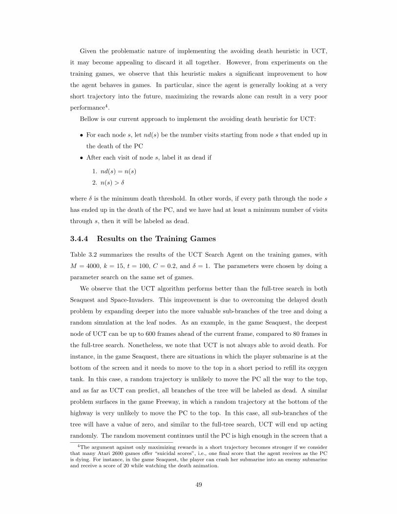
Given the problematic nature of implementing the avoiding death heuristic in UCT,

it may become appealing to discard it all together. However, from experiments on the

training games, we observe that this heuristic makes a significant improvement to how

the agent behaves in games. In particular, since the agent is generally looking at a very

short trajectory into the future, maximizing the rewards alone can result in a very poor

performance4.

Bellow is our current approach to implement the avoiding death heuristic for UCT:

• For each node s, let nd(s) be the number visits starting from node s that ended up in

the death of the PC

• After each visit of node s, label it as dead if

1. nd(s) = n(s)

2. n(s) > δ

where δ is the minimum death threshold. In other words, if every path through the node s

has ended up in the death of the PC, and we have had at least a minimum number of visits

through s, then it will be labeled as dead.

3.4.4 Results on the Training Games

Table 3.2 summarizes the results of the UCT Search Agent on the training games, with

M = 4000, k = 15, t = 100, C = 0.2, and δ = 1. The parameters were chosen by doing a

parameter search on the same set of games.

We observe that the UCT algorithm performs better than the full-tree search in both

Seaquest and Space-Invaders. This improvement is due to overcoming the delayed death

problem by expanding deeper into the more valuable sub-branches of the tree and doing a

random simulation at the leaf nodes. As an example, in the game Seaquest, the deepest

node of UCT can be up to 600 frames ahead of the current frame, compared to 80 frames in

the full-tree search. Nonetheless, we note that UCT is not always able to avoid death. For

instance, in the game Seaquest, there are situations in which the player submarine is at the

bottom of the screen and it needs to move to the top in a short period to refill its oxygen

tank. In this case, a random trajectory is unlikely to move the PC all the way to the top,

and as far as UCT can predict, all branches of the tree will be labeled as dead. A similar

problem surfaces in the game Freeway, in which a random trajectory at the bottom of the

highway is very unlikely to move the PC to the top. In this case, all sub-branches of the

tree will have a value of zero, and similar to the full-tree search, UCT will end up acting

randomly. The random movement continues until the PC is high enough in the screen that a4The argument against only maximizing rewards in a short trajectory becomes stronger if we consider

that many Atari 2600 games offer “suicidal scores”, i.e., one final score that the agent receives as the PCis dying. For instance, in the game Seaquest, the player can crash her submarine into an enemy submarineand receive a score of 20 while watching the death animation.

49

Game Average Reward per EpisodeUCT Full-Tree Search Best-Action Random Author

Asterix 1814† 1980† 250 156 1380Freeway 5.2† 2.7 5 0 12.4Seaquest 573† 161† 41 27 1286SpaceInvaders 625† 417† 92 59 458

Table 3.2: Results of the UCT search-agent on training games, compared to the Full-treesearch, Best-Action and Random agents. Rewards are averaged over 100 episodes. Resultsspecified by † are significantly higher than both Best-Action and Random agents results(p = 0.05).

random trajectory reaches the top of the highway and receives a positive reward. Finally, we

note that UCT is performing slightly worst than the full-tree search in the game Asterix. In

this game both the rewards and the PC death is within the reach of the full-tree expansion.

The random simulations performed at the leaf nodes do not gain much for UCT, but limit

it to expanding a smaller tree compared to the full-tree search.

In summary, when a random trajectory is able to receive rewards and both detect and

avoid the death of the PC, a search-base agent using UCT performs well. On the other

hand, when a random simulation does not receive any rewards (as in Freeway) or cannot

avoid death (as in Seaquest), UCT will perform poorly.

3.5 Discussion

This section illustrated how we can generate a state-action tree for any Atari 2600 game,

using save-state/restore-state features of the emulator, and how full-tree search and UCT

perform on the training games. It is important to note that while only two search methods

are presented here, the Atari 2600 console and its plentiful game library can now be used

by the AI community as a platform for developing and testing various new search methods.

Combining the search techniques presented here with the learning techniques discussed

in previous sections is an interesting future direction for this research. In particular, in

many games, the search-based agent gives us a policy that if not the same as π∗, still out

performs a typical human player. The question is how we can use this good policy to either

learn faster or learn to perform better in the RL-based methods. A number of approaches

for combining the learning and search methods will be discussed in Chapter 5.

50

Chapter 4

Evaluation Method andExperimental Results

This chapter contains an overview of our evaluation method, including the process of choos-

ing the test games, a brief introduction to the emulation software, and the details of the

experimental setup. The experimental results on the test games, as well as a number of

observations on how certain game properties impact the performance of different agents is

also presented.

4.1 Training and Test Games

To insure the generic nature of the methods developed in this thesis, the set of games that is

used for designing and fine-tuning the agents is separated from the set of games that is used

for their final evaluation. The first set, referred to as the training games, consists of four

games: Asterix, Freeway, Seaquest, and Space Invaders1. The performance of the agents on

these games is used for parameter search as well as overall design refinements.

The test games are a set of 50 games, used for the final evaluation of our agents. These

games were randomly selected from a larger set of Atari 2600 games after the development

process and parameter search for all agents was completed. To choose the test games, we

started from the List of Atari Games in Wikipedia (August 18, 2009)2. Of the 595 games

listed here, 123 games that have their own Wikipedia page, have a single player mode, are

not adult themed or prototypes, and can be emulated in our learning environment were

selected. From this list, 50 games were randomly picked and added to the test games.

4.2 Emulation Software

To simplify the implementation of the five AI agents and the task of evaluating them on

54 training and test games, we developed ALE (Atari 2600 Learning Environment). Built1Appendix B provides a short description for each of the training games.2http://en.wikipedia.org/w/index.php?title=List of Atari 2600 games&oldid=308675482

51

on top of Stella, a popular Atari 2600 emulator, ALE provides a simple object-oriented

framework that separates the AI development from the low-level details of Atari 2600 games

and the emulation process. ALE also uncouples the emulation core from the rendering and

sound generation modules of Stella. This enables fast emulation on clusters with minimum

library dependencies3.

The game score is retrieved from the console RAM. To do this, the location of the game

score needs to be manually extracted. In games like Boxing, in which the agent is playing

against an AI opponent, the reward is calculated by subtracting the opponent score from

the player score. The end of the game is usually detected by monitoring the number of lives

the player has left. When this number decreases, the game is declared over and the current

episode ends. Note that there may be a delay of up to 200 frames between the time that

the player character dies and when the number of lives is actually decreased. As it will be

discussed in section 4.4, this death delay has a significant impact on the performance of both

of the RL-based and search-based agents.

4.3 Experimental Setup

The learning task is episodic. A new episode starts on the frame in which the player begins

acting in the game. That is, the opening animation of the games are left out. Episodes

end either when the game is over (e.g., when the PC dies) or after 1800 frames of game

play. The RL-based agents interact with each game for 1.8 × 107 frames (i.e., a minimum

of 10000 episodes). The average reward over the last 1000 episodes is reported as the final

performance of an RL-based agent. Since there is no learning involved in the search-based

agents and their performance generally has a smaller variance compared to the RL-based

agents, the reported performance for the search-based agents is the average reward over 100

episodes4.

4.4 Results on the Test Games

The performance results of all the agents on the test games is summarized in table 4.1.

All five agents outperform the Random agent in over half of the games. For the RL-based

agents, this result indicates that significant learning has in fact taken place. The percentage

of the test games in which each agent performs significantly better than the Random and the

Best-Action agents is presented in Table 4.2. The search-based agents achieve human-level

performance in a number of games. Table 4.3 presents four games in which the search-based3ALE is released as free and open source software under the terms of the GNU General Public License.

For further information please visit: http://yavar.naddaf.name/ale4The search-based agents are also much slower than the RL-based agents, running at about 2 frames per

second. Running a search-based agent on a single game for 100 episodes already takes more than 24 hoursof simulation time.

52

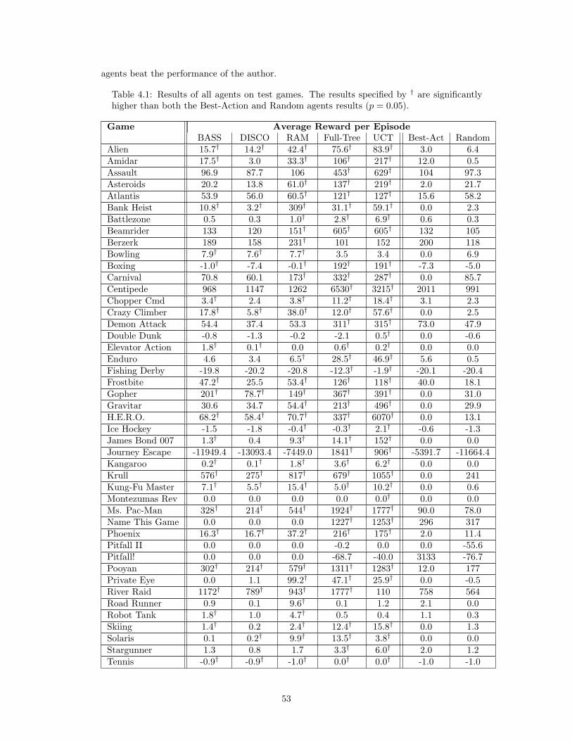
agents beat the performance of the author.

Table 4.1: Results of all agents on test games. The results specified by † are significantlyhigher than both the Best-Action and Random agents results (p = 0.05).

Game Average Reward per EpisodeBASS DISCO RAM Full-Tree UCT Best-Act Random

Alien 15.7† 14.2† 42.4† 75.6† 83.9† 3.0 6.4Amidar 17.5† 3.0 33.3† 106† 217† 12.0 0.5Assault 96.9 87.7 106 453† 629† 104 97.3Asteroids 20.2 13.8 61.0† 137† 219† 2.0 21.7Atlantis 53.9 56.0 60.5† 121† 127† 15.6 58.2Bank Heist 10.8† 3.2† 309† 31.1† 59.1† 0.0 2.3Battlezone 0.5 0.3 1.0† 2.8† 6.9† 0.6 0.3Beamrider 133 120 151† 605† 605† 132 105Berzerk 189 158 231† 101 152 200 118Bowling 7.9† 7.6† 7.7† 3.5 3.4 0.0 6.9Boxing -1.0† -7.4 -0.1† 192† 191† -7.3 -5.0Carnival 70.8 60.1 173† 332† 287† 0.0 85.7Centipede 968 1147 1262 6530† 3215† 2011 991Chopper Cmd 3.4† 2.4 3.8† 11.2† 18.4† 3.1 2.3Crazy Climber 17.8† 5.8† 38.0† 12.0† 57.6† 0.0 2.5Demon Attack 54.4 37.4 53.3 311† 315† 73.0 47.9Double Dunk -0.8 -1.3 -0.2 -2.1 0.5† 0.0 -0.6Elevator Action 1.8† 0.1† 0.0 0.6† 0.2† 0.0 0.0Enduro 4.6 3.4 6.5† 28.5† 46.9† 5.6 0.5Fishing Derby -19.8 -20.2 -20.8 -12.3† -1.9† -20.1 -20.4Frostbite 47.2† 25.5 53.4† 126† 118† 40.0 18.1Gopher 201† 78.7† 149† 367† 391† 0.0 31.0Gravitar 30.6 34.7 54.4† 213† 496† 0.0 29.9H.E.R.O. 68.2† 58.4† 70.7† 337† 6070† 0.0 13.1Ice Hockey -1.5 -1.8 -0.4† -0.3† 2.1† -0.6 -1.3James Bond 007 1.3† 0.4 9.3† 14.1† 152† 0.0 0.0Journey Escape -11949.4 -13093.4 -7449.0 1841† 906† -5391.7 -11664.4Kangaroo 0.2† 0.1† 1.8† 3.6† 6.2† 0.0 0.0Krull 576† 275† 817† 679† 1055† 0.0 241Kung-Fu Master 7.1† 5.5† 15.4† 5.0† 10.2† 0.0 0.6Montezumas Rev 0.0 0.0 0.0 0.0 0.0† 0.0 0.0Ms. Pac-Man 328† 214† 544† 1924† 1777† 90.0 78.0Name This Game 0.0 0.0 0.0 1227† 1253† 296 317Phoenix 16.3† 16.7† 37.2† 216† 175† 2.0 11.4Pitfall II 0.0 0.0 0.0 -0.2 0.0 0.0 -55.6Pitfall! 0.0 0.0 0.0 -68.7 -40.0 3133 -76.7Pooyan 302† 214† 579† 1311† 1283† 12.0 177Private Eye 0.0 1.1 99.2† 47.1† 25.9† 0.0 -0.5River Raid 1172† 789† 943† 1777† 110 758 564Road Runner 0.9 0.1 9.6† 0.1 1.2 2.1 0.0Robot Tank 1.8† 1.0 4.7† 0.5 0.4 1.1 0.3Skiing 1.4† 0.2 2.4† 12.4† 15.8† 0.0 1.3Solaris 0.1 0.2† 9.9† 13.5† 3.8† 0.0 0.0Stargunner 1.3 0.8 1.7 3.3† 6.0† 2.0 1.2Tennis -0.9† -0.9† -1.0† 0.0† 0.0† -1.0 -1.0

53

Table 4.1: Results of all agents on test games. The results specified by † are significantlyhigher than both the Best-Action and Random agents results (p = 0.05).

Game Average Reward per EpisodeBASS DISCO RAM Full-Tree UCT Best-Act Random

Time Pilot 2.1 2.0 3.0† 21.2† 25.6† 0.9 2.2Tutankham 15.5† 17.3† 43.7† 53.7† 61.7† 0.0 4.2Up’n Down 254 109 531† 2390† 5273† 254 43.6Video Pinball 1853 1417 2051 2674† 3032† 1331 2105Zaxxon 2.4† 0.0† 0.2† 1.2† 0.6† 0.0 0.0

Generally speaking, the performance of all agents compared to the Best-Action agent

is slightly worst than their relative performance to the Random agent. In many games

repeating the same action obtains considerable amounts of rewards (e.g., always going up

in Freeway or always pressing Fire in River Raid). Outperforming this result can be a

nontrivial and challenging task. As an informal observation, we note that in the game

River Raid, human players often do not reach the second stage of the game on their first

few trials. On the other hand, just pressing the Fire button always reaches the second

stage. This results suggest that policy search reinforcement learning methods may be good

candidates for learning in the Atari 2600 domain.

The search-based agents generally outperform the RL-based agents. This is expected,

since the learning problem is generally more difficult than the search problem. The search-

based agents have access to a fully generative model of each game, which allows them to

simulate the consequences of their actions into the future. The RL-based agents do not

have access to the full dynamics of the game, and can only see the consequences of the

actions that were previously taken. The main challenge of the search problem is to address

the exploration/exploitation problem in order to maximize the look-ahead horizon. The

learning-based agents also need to deal with the exploration/exploitation problem. However,

the learning problem also involves learning a mapping from each state to the expected future

rewards in that state. This introduces a whole new set of challenges, including feature

generation and function approximation.

Compared to the full-tree search, UCT gets significantly better results in over half of

the games (p = 0.05). This is because the full expansion of the state-action tree limits

the full-tree search agent to a very short look-ahead horizon. On the other hand, UCT

simulates deeper into the more promising branches of the tree and therefore usually has a

longer look-ahead trajectory.

Among the RL-based agents, the RAM-agent has the highest overall performance. A

possible explanation for this is that the content of the console memory is inherently Markov,

i.e., the content of the RAM is a state that contains all relevant game information from the

past. As discussed in Section 2.8.4, this is not always the case in the other RL-based

54

Agent OutperformsRandom Best-Action Both

BASS 72% 56% 56%DISCO 56% 48% 42%RAM 90% 74% 76%Full-Tree 88% 86% 84%UCT 94% 88% 86%

Table 4.2: The percentage of the test games in which each agent performs significantlybetter than the Random and Best-Action agents

Game Average Reward per EpisodeFull-Tree Search UCT Author

Beam Rider 604.9 605.3 457Boxing 192 191 3Centipede 6530 3215 1876Up and Down 2390 5272 898

Table 4.3: Search-based agents with human-level performance

methods. Aside from the Markov property, it could also be the case that compared to

the feature vectors generated from the game screens, the console RAM provides a better

representation of the important features of the games.

4.5 Impact of Game Properties on Agents Performance

To understand the varying performance of the agents on different games, we look at a

number of game properties and how they impact the performance of the learning and search

based methods. Some of the properties considered are related to the specific assumptions

made by the methods (e.g., important game entities having distinct colors in BASS), while

others are well-established challenges in general learning and planning tasks (e.g., having

delayed rewards). Table 4.4 contains the full list of extracted properties for the test games.

We note that not all of the game properties have a well defined and concrete definition, and

some can be rather subjective. Bellow is a short description for each column:

• SB (Static Background): True in games in which the majority of the game screen has

a static and non-scrolling background.

• FC: True when the important game entities belong to a few classes of 2D objects

• DC: True when the important game entities have distinct colors in the SECAM

palette.

• PF: True when all game entities are present on every frame. Some Atari-2600 games

draw the game entities on alternating frames to save processing power. For these

games, this property will be false.

55

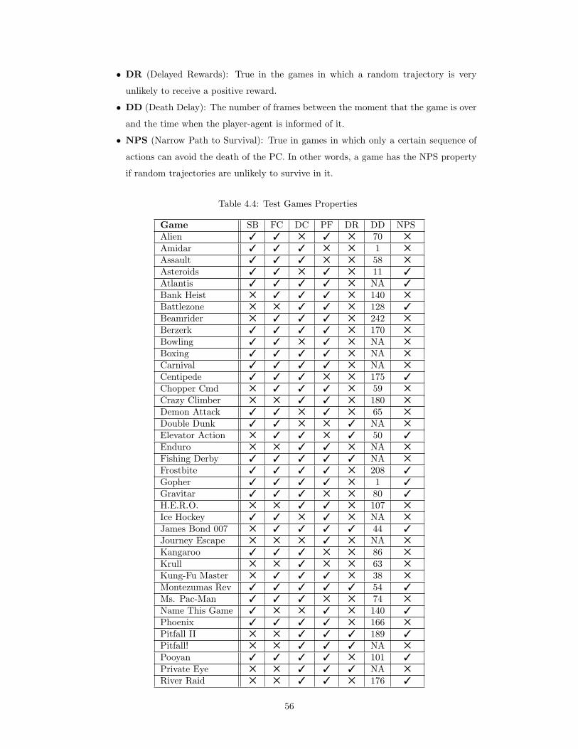
• DR (Delayed Rewards): True in the games in which a random trajectory is very

unlikely to receive a positive reward.

• DD (Death Delay): The number of frames between the moment that the game is over

and the time when the player-agent is informed of it.

• NPS (Narrow Path to Survival): True in games in which only a certain sequence of

actions can avoid the death of the PC. In other words, a game has the NPS property

if random trajectories are unlikely to survive in it.

Table 4.4: Test Games Properties

Game SB FC DC PF DR DD NPSAlien 3 3 5 3 5 70 5

Amidar 3 3 3 5 5 1 5

Assault 3 3 3 5 5 58 5

Asteroids 3 3 5 3 5 11 3

Atlantis 3 3 3 3 5 NA 3

Bank Heist 5 3 3 3 5 140 5

Battlezone 5 5 3 3 5 128 3

Beamrider 5 3 3 3 5 242 5

Berzerk 3 3 3 3 5 170 5

Bowling 3 3 5 3 5 NA 5

Boxing 3 3 3 3 5 NA 5

Carnival 3 3 3 3 5 NA 5

Centipede 3 3 3 5 5 175 3

Chopper Cmd 5 3 3 3 5 59 5

Crazy Climber 5 5 3 3 5 180 5

Demon Attack 3 3 5 3 5 65 5

Double Dunk 3 3 5 5 3 NA 5

Elevator Action 5 3 3 5 3 50 3

Enduro 5 5 3 3 5 NA 5

Fishing Derby 3 3 3 3 3 NA 5

Frostbite 3 3 3 3 5 208 3

Gopher 3 3 3 3 5 1 3

Gravitar 3 3 3 5 5 80 3

H.E.R.O. 5 5 3 3 5 107 5

Ice Hockey 3 3 5 3 5 NA 5

James Bond 007 5 3 3 3 3 44 3

Journey Escape 5 5 5 3 5 NA 5

Kangaroo 3 3 3 5 5 86 5

Krull 5 5 3 5 5 63 5

Kung-Fu Master 5 3 3 3 5 38 5

Montezumas Rev 3 3 3 3 3 54 3

Ms. Pac-Man 3 3 3 5 5 74 5

Name This Game 3 5 5 3 5 140 3

Phoenix 3 3 3 3 5 166 5

Pitfall II 5 5 3 3 3 189 3

Pitfall! 5 5 3 3 3 NA 5

Pooyan 3 3 3 3 5 101 3

Private Eye 5 5 3 3 3 NA 5

River Raid 5 5 3 3 5 176 3

56

Table 4.4: Test Games Properties

Game SB FC DC PF DR DD NPSRoad Runner 3 3 3 3 5 147 3

Robot Tank 5 5 3 3 5 140 3

Skiing 3 3 3 3 5 NA 5

Solaris 5 5 3 3 3 40 5

Stargunner 3 3 5 3 5 130 5

Tennis 3 3 3 3 3 NA 3

Time Pilot 3 3 5 5 5 201 5

Tutankham 5 5 3 5 5 86 5

Up’n Down 5 5 3 5 5 197 3

Video Pinball 3 3 3 3 5 1 5

Zaxxon 5 5 3 3 3 126 3

While various patterns can be extracted from this data, most of the relations are not

statistically significant with the current number of test games. For instance, having all game

entities present on every frame does seem to have a positive impact on the performance of

both the BASS and DISCO agents, i.e., agents with feature vectors generated from the game

screens. However, since the difference is not statistically significant at an acceptable level,

this could very well be a random pattern. Below, we list three properties that do have a

statistically significant (p = 0.07) impact on the performance of one or more of the player

agents:

1. As expected, the BASS agent performs better in games in which the important game

entities have distinct colors under the SECAM palette. It performs better than both

the Random agent and the Best-Action agent in 65% of games in which entities have

distinct colors, as opposed to only 20% of games that do not have this property.

2. The death delay, i.e., the number of frames between the moment that the game is over

and the time when the player-agent is informed of it, has a negative impact on the

performance of the search-based agents. This is particularly true for the UCT agent,

in which there is a significant correlation of −0.35 between the number of frames in

the death delay and the probability of winning against both Random and Best-Action

agents. A similar correlation (-0.25) holds for the Full-Tree search agent, however it

is not statistically significant.

3. As discussed in sections 2.8.2 and 3.4.4, having delayed rewards5 is a major challenge

for both learning and search based methods. This is confirmed by the results from the

test games. As Table 4.5 illustrates, all agents perform better in games that do not

have delayed rewards.

5Games with delayed rewards are games in which the agent receives rewards of zero in most of the states,and only receives a non-zero reward after it has executed a complex sequence of actions. Here, to have amore concrete definition, we only consider a game to have delayed rewards if random trajectories are veryunlikely to receive positive rewards in it.

57

BASS DISCO RAM Full-Tree UCTGames With Delayed Rewards 30% 30% 50% 60% 80%Games Without Delayed Rewards 62% 53% 80% 93% 90%

Table 4.5: Comparison of the performance of the agents on games with and without delayedrewards. Each cell value presents the percentage of the games in which the given agent per-forms better than the Best-Action agent. Columns with a statistically significant differencebetween the two values are printed in bold.

The extracted game properties also allow us to make an observation on the type of games

in which the RL-agents outperform the search-based agents. As mentioned in the previous

section, the search-based agents generally outperform the RL-based agents. However, there

are still a number of games in which the RL-based agents perform better than the search-

based agents. Most of these games can be categorized into two groups:

1. Games in which a random trajectory is not likely to receive rewards, e.g., Elevator

Action and Private Eye.

2. Games in which the death delay is large, e.g., Bank Heist, Berzerk, Road Runner, and

Robotank.

Search-based agents perform well when the look-ahead trajectory is able to receive rewards

and both detect and avoid the death of the PC. Since there is no learning involved, when

either the reward or the end of the game is not detectable in the look-ahead horizon, the

search-based agents perform poorly. Additional interactions with the game does not improve

the performance of a search-based agent. The RL-based agents, on the other hand, are able

to do value propagation which allows them to broadcast the value of delayed rewards and

delayed consequences to previous states. Delayed rewards and delayed consequences are still

challenging obstacles, but the RL-agents have a chance of overcoming them over time.

58

Chapter 5

Conclusion and Future Work

This thesis introduced the Atari 2600 as an attractive platform for developing and evaluating

AI algorithms. Three reinforcement learning agents were developed that use features from

the game screen as well as the console RAM to learn to play generic Atari 2600 games.

Furthermore, it was demonstrated how by using the save-state/restore-state features of the

emulator, a state-action tree can be generated for any Atari 2600 game. Full-tree search

as well as UCT was applied on the generated trees, aiming to play as well as possible by

only exploring a very small fraction of the large state-space. To insure the generic nature

of our methods, four specific games were used to design and fine-tune the agents, and later

fifty randomly chosen games were used for evaluating their performance. The experimental

results show that significant learning has taken place in the RL-based agents, while the

search-based agents achieve human-level performance in a number of games. Among the

RL-based agents, the RAM agent has the best performance, possibly because it is the only

RL-agent with truly Markov states. The results also show that UCT performs significantly

better than the full-tree search in over half of the games. While the search-based agents

generally outperform the RL-based agents, there are still a number of games (mainly those

with either delayed rewards or large death delays) in which the RL-based agents perform

better. Finally, the results show that the death delay and delayed rewards have a significant

negative impact on the performance of the player agents, making these important challenges

for ongoing research. Sensitivity to the learning rate (α) and having to deal with complex

value functions and Non-Markovian states are other critical obstacles for the learning agents.

This work has only started to scratch the surface of the problem of playing generic Atari

2600 games. A number of possible future directions for this research are discussed bellow:

• The large and diverse set of test games, with wide range of reward functions and state

transition dynamics, provide an excellent opportunity for a comprehensive comparison

between various RL methods. All three RL-based agents in this thesis use Sarsa(λ) as

their learning method. It will be interesting to investigate how other Reinforcement

59

Algorithms compare with Sarsa(λ), when applied on the same feature vectors and run

on the same set of games.

• Sensitivity to the learning rate (α) is a major setback in our RL-based agents. Our

experiments with meta-learning methods such as Delta-bar-Delta and iDBD does not

seem to improve this problem. We note that the Atari 2600, with a substantial num-

ber of games each having a unique reward structure and value function, is an excel-

lent platform for developing and testing new meta-learning methods for reinforcement

learning.

• The RL-based agents need to deal with large and sparse feature vectors, with only a

small fraction of the features being important for approximating the value function.

These properties make the learning problem in Atari 2600 games an excellent candi-

date for applying regularized reinforcement learning methods [Farahmand et al., 2009,

Loth and Davy, 2007].

• Combining the search-based and the RL-based methods is another exciting future

direction for this research. In particular, in many games the search-based agents

generate policies that if not optimal, still play on the level of a typical human player.

The question is how these good policies can be used to help the RL-based methods

either learn faster or learn to perform better.

A simple approach for integrating the search and learning methods is to do a short

look-ahead search before choosing an action in the reinforcement learning methods.

When choosing a greedy action at time step t, instead of returning the action that

maximizes Qt(st, a), we can generate a small state-action tree with its root at st and

return the action associated to the branch with the highest value. This is similar to

the method employed by Tesauro in TD-Gammon [Tesauro, 2002], in which a k-ply

search is performed before returning an action. Tesauro also uses the value function

learned by the TD method to forward prune the search tree.

The Dyna-2 algorithm [Silver et al., 2008] presents another approach for combining

the learning and search methods. In Dyna-2, the agent estimates two value functions:

the first one, referred two as the permanent learning memory, is updated from real

experience, and the second one, called the transient planning memory, is updated

from simulated experience. The permanent memory is updated similar to the Sarsa

algorithm. Additionally, at each state the agent performs a local sample-based search

and updates its transient memory. A greedy action is then selected from a linear

combination of both the permanent and transient memories.

Learning Real Time A* (LRTA*) [Korf, 1990], a real time heuristic search which up-

dates its heuristic estimates on every step, is another possible approach for combining

60

the search and learning methods. In LRTA*, the agent starts with an initial heuristic

function. On each step, the agent acts greedily based on the current heuristic func-

tion. LRTA* then updates the heuristic estimate for the previous state based on the

heuristic value of the new state.

Offline batch supervised learning is yet another possible approach for integrating the

search and learning methods. A set of samples can be collected from a search-agent

playing a given game. A supervised method can then be applied to learn a mapping

from the feature vectors to the actions taken. The resulting classification model can

be used to generate an imitation agent.

61

Appendix A

Video Game Terminology

Bellow, we provide a short definition for some of the video game related terminology used

through the thesis:

Video Game Console: Computer systems designed specifically for playing video

games. Unlike the generic Personal Computers, game consoles often do not allow

users to install arbitrary software. They also usually do not provide a keyboard and

mouse interface, and interaction with the system is only through the provided game

controllers. To this date, there has been seven generations of videogame consoles,

starting from the Pong in the first generation to the Wii, Xbox 360 and PlayStation

3 in the seventh (current) generation.

Emulator: “A piece of hardware/software that allows a user to execute game software

on a platform for which the software was not originally intended. For example, video

game emulators allow a personal computer to function almost identically to a video

game console or an arcade game system”. [Conley et al., 2004]

Save-State: Saving the current state of a game by dumping the content of RAM.

Console emulators often implement save-state (also known as freeze-state) to let players

save their games even when the game or the system does not provide a save feature.

Restore-State: Loading the state of a game from a RAM dump previously saved

through save-state.

Game Cartridge (a.k.a Game ROM): A removable cartridge with a Read-Only

Memory device, containing the binary content of a console game. Some game car-

tridges may also include additional RAM or hardware expansions.

Player Character (PC): The character in a game that is controlled by the player.

Non-Player Character (NPC): A character in a game that is not controlled by the

player. NPC’s can be enemies or allies.

62

Appendix B

Description of the TrainingGames

This section provides a short description for each of the four training games. The descrip-

tions are useful to better understand some of the examples provided through the thesis.

Figure 1.1 contains a screenshot for each of the four games.

B.1 Asterix

Asterix is an Atari 2600 video game, developed by Steve Woita and published by Atari in

1982. Released for the European market, the game is essentially a slightly modified version

of the Atari 2600 game Tad. The player controls the Asterix’s character. The aim of the

game is to collect the sprites resembling magic potions while avoiding the sprites resembling

lyres. Each time Asterix collects a magic potion, the player receives a score of 50. The

game is over when the player character is hit by a lyre. There are five possible actions in

the game: Up, Down, Left, Right, and No-Action.

B.2 Freeway

Freeway is an Atari 2600 video game, developed by David Crane and published by Activision

in 1981. The gameplay is very similar to the popular arcade game Frogger. The player

controls the yellow chicken, and the goal of the game is to reach the top of the highway

while avoiding the passing cars. Once the chicken reaches the top of the highway, the player

receives a score of one, and the chicken moves back to the bottom of the screen. In the

hard mode, in which we run our experiments, when the chicken is hit by a car, it moves all

the way back to the bottom of the highway and needs to start again. The player character

never dies, and the game only ends after two minutes of gameplay. There are three possible

actions in the game: Up, Down, and No-Action.

63

B.3 Seaquest

Seaquest is an Atari 2600 video game, developed by Steve Cartwright and published by

Activision in 1982. The player controls a yellow submarine, and the goal of the game is

to destroy waves of coming sharks and enemy submarines, while rescuing the swimming

divers who are being chased by the sharks. The submarine has a limited supply of oxygen,

displayed as a shrinking white bar at the bottom of the screen. If the oxygen supply reaches

zero, the player submarine explodes and the game ends. To resupply on oxygen, the player

needs to bring up the submarine to the surface. The player receives a score of 20 for killing

a shark or destroying an enemy submarine. The game does not award any immediate scores

for rescuing divers. However, the rescued divers are important in two ways. First, they

are essential for resupplying on oxygen at the surface. If the player has rescued at least

one diver, bringing the submarine to the surface will consume one of the divers and the

player receives a full tank of oxygen. If the player has not rescued any divers, once the

submarine reaches the surface, it will explode and the game ends. Also, collecting six divers

(without losing any of them for resupplying on oxygen) and coming up to the surface results

in a large score of 1000. The game ends when the oxygen supply reaches zero or if the

player submarine is hit by either a shark, an enemy submarine, or bullets from the enemy

submarines. There are ten possible actions in the game: Up, Down, Left, Right, Up-Fire,

Down-Fire, Left-Fire, Right-Fire, Fire, and No-Action.

B.4 Space Invaders

Space Invaders on the Atari 2600 is a port from the popular arcade video game designed by

Tomohiro Nishikado, and released in 1978. The player controls a laser cannon at the bottom

of the screen that can be moves to the left and right. The aim of the game is to destroy the

48 space aliens before they reach the bottom of the screen. The aliens move horizontally and

randomly fire bullets toward the bottom. There is a different score associated for destroying

aliens from different rows: 5 in the first row, 10 in the second row, until 30 scores for the

sixth row. The game ends if an alien reaches the bottom of the screen or the or the player

character is hit by an alien bullet. We note that there is a bug when emulating Space

Invaders in Stella, and not all game entities are rendered on all frames. In particular, the

alien bullets and the protective barriers are often missing from the screen for several seconds.

64

Appendix C

Atari 2600 TechnicalSpecifications

Bellow is a brief description of the Atari 2600 hardware specification. For a more detailed

description, please see [Montfort and Bogost, 2009].

• Release Date: October 1977

• CPU: 8bit, 6507 MOS Technology

• CPU Clock: 1.19 MHz

• RAM: 128 bytes

• ROM: External game cartridge. 4KB maximum capacity (more can be addressed via

bank switching)

• Resolution: 160 × 192 pixels

• Colors: 128 colors (NTSC palette), 104 colors(PAL palette), 8 colors (SECAM palette)

• Sound: 2 channel mono sound (with frequency, volume, noise control)

Figure C.1: The Atari 2600 Video Computer System

65

Bibliography

[Balla and Fern, 2009] Balla, R.-K. and Fern, A. (2009). UCT for tactical assault plan-ning in real-time strategy games. In Proceedings of the twenty-first international jointconference on Artifical Intelligence.

[Bowling et al., 2009] Bowling, M., Risk, N. A., Bard, N., Billings, D., Burch, N., Davidson,J., Hawkin, J., Holte, R., Johanson, M., Kan, M., Paradis, B., Schaeffer, J., Schnizlein,D., Szafron, D., Waugh, K., and Zinkevich, M. (2009). A demonstration of the Polarispoker system. In Proceedings of The Eighth International Conference on AutonomousAgents and Multiagent Systems.

[Buro, 2004] Buro, M. (2004). Call for AI research in RTS games. In Proceedings of theNineteenth National Conference on Artificial Intelligence Workshop on Challenges inGame AI.

[Campbell et al., 2002] Campbell, M., Hoane, Jr., A. J., and Hsu, F.-h. (2002). Deep blue.Artificial Intelligence, 134(1-2):57–83.

[Clune, 2007] Clune, J. (2007). Heuristic evaluation functions for general game playing. InProceedings of the twenty-second national conference on Artificial Intelligence.

[Conley et al., 2004] Conley, J., Andros, E., Chinai, P., Lipkowitz, E., and Perez, D. (2004).Use of a game over: Emulation and the video game industry. Northwestern Journal ofTechnology and Intellectual Property, 2(2).

[Conn and Peters, 2007] Conn, K. and Peters, R. A. (2007). Reinforcement learning witha supervisor for a mobile robot in a real-world environment. In Proceedings of the IEEEInternational Symposium on Computational Intelligence in Robotics and Automation.

[Cutumisu et al., 2008] Cutumisu, M., Szafron, D., Bowling, M., and Sutton, R. S. (2008).Agent learning using action-dependent learning rates in computer role-playing games.In Proceedings of the Fourth Conference on Artificial Intelligence and Interactive DigitalEntertainment (AIIDE).

[Diuk et al., 2008] Diuk, C., Cohen, A., and Littman, M. L. (2008). An object-orientedrepresentation for efficient reinforcement learning. In Proceedings of the twenty-fifth in-ternational conference on Machine learning.

[Farahmand et al., 2009] Farahmand, A.-M., Ghavamzadeh, M., Szepesvari, C., and Man-nor, S. (2009). Regularized fitted Q-iteration for planning in continuous-space markoviandecision problems. In Proceedings of American Control Conference (ACC).

[Forsyth and Ponce, 2002] Forsyth, D. A. and Ponce, J. (2002). Computer Vision: A Mod-ern Approach. Prentice Hall Professional Technical Reference.

[Genesereth and Love, 2005] Genesereth, M. and Love, N. (2005). General game playing:Overview of the AAAI competition. AI Magazine, 26:62–72.

[Haslum et al., 2005] Haslum, P., Bonet, B., and Geffner, H. (2005). New admissible heuris-tics for domain-independent planning. In Proceedings of the Twentieth national conferenceon Artificial Intelligence.

[Horn, 1986] Horn, B. K. (1986). Robot Vision. McGraw-Hill Higher Education.

[Jacobs, 1987] Jacobs, R. A. (1987). Increased rates of convergence through learning rateadaptation. Technical Report UM-CS-1987-117, University of Massachusetts.

66

[Kocsis and Szepesvari, 2006] Kocsis, L. and Szepesvari, C. (2006). Bandit based Monte-Carlo planning. In Proceedings of the Fifteenth European Conference on Machine Learning(ECML).

[Korf, 1990] Korf, R. E. (1990). Real-time heuristic search. Artificial Intelligence, 42(2-3):189–211.

[Laird and Lent, 2000] Laird, J. E. and Lent, M. v. (2000). Human-level AI’s killer applica-tion: Interactive computer games. In Proceedings of the Seventeenth National Conferenceon Artificial Intelligence and Twelfth Conference on Innovative Applications of ArtificialIntelligence.

[Laud and DeJong, 2003] Laud, A. and DeJong, G. (2003). The influence of reward on thespeed of reinforcement learning: An analysis of shaping. In Proceedings of the TwentiethInternational Conference on Machine Learning (ICML).

[Loth and Davy, 2007] Loth, M. and Davy, M. (2007). Sparse temporal difference learningusing lasso. In IEEE International Symposium on Approximate Dynamic Programmingand Reinforcement Learning.

[Lucas, 2009] Lucas, S. M. (2009). Computational Intelligence and AI in games: A newIEEE transactions. IEEE Transactions on Computational Intelligence and AI in Games,1(1):1–3.

[Luders, 2007] Luders, R. A. (2007). Control strategies for a multi-legged hopping robot.Master’s thesis, Robotics Institute, Carnegie Mellon University.

[McPartland and Gallagher, 2008] McPartland, M. and Gallagher, M. (2008). Learning tobe a bot: Reinforcement learning in shooter games. In Proceedings of the fourth ArtificialIntelligence in Interactive Digital Entertainment (AIIDE).

[Michael Chung, 2005] Michael Chung, Michael Buro, J. S. (2005). Monte Carlo planningin RTS games. In Proceedings of the IEEE Symposium on Computational Intelligence andGames.

[Mohan and Laird, 2009] Mohan, S. and Laird, J. E. (2009). Learning to play Mario. Tech-nical Report CCA-TR-2009-03, Center for Cognitive Architecture, University of Michigan.

[Montfort and Bogost, 2009] Montfort, N. and Bogost, I. (2009). Racing the Beam: TheAtari Video Computer System. The MIT Press.

[Ponsen, 2004] Ponsen, M. (2004). Improving Adaptive Game AI with Evolutionary Learn-ing. Master’s thesis, Delft University of Technology.

[Ponsen et al., 2006] Ponsen, M., Spronck, P., and Tuyls, K. (2006). Towards relationalhierarchical reinforcement learning in computer games. In Proceedings of the EighteenthBenelux Conference on Artificial Intelligence.

[Randløv and Alstrøm, 1998] Randløv, J. and Alstrøm, P. (1998). Learning to drive a bicy-cle using reinforcement learning and shaping. In Proceedings of the Fifteenth InternationalConference on Machine Learning (ICML).

[Schaeffer et al., 2005] Schaeffer, J., Bjrnsson, Y., Burch, N., Kishimoto, A., Mller, M.,Lake, R., Lu, P., and Sutphen, S. (2005). Solving checkers. In Proceedings of the Nine-teenth International Joint Conference on Artificial Intelligence (IJCAI-05.

[Shafiei et al., 2009] Shafiei, M., Sturtevant, N., and Schaeffer, J. (2009). Comparing UCTversus CFR in simultaneous games. In Proceedings of the Twenty-First International JointConferences on Artificial Intelligence Workshop on General Game Playing (GIGA’09).

[Silver et al., 2008] Silver, D., Sutton, R. S., and Muller, M. (2008). Sample-based learningand search with permanent and transient memories. In Proceedings of the twenty-fifthInternational Conference on Machine Learning.

[Smith et al., 2007] Smith, M., Lee-Urban, S., and Munoz-Avila, H. (2007). RETALIATE:learning winning policies in first-person shooter games. In Proceedings of the ninetiethnational conference on Innovative applications of Artificial Intelligence.

67

[Spronck et al., 2006] Spronck, P., Ponsen, M., Sprinkhuizen-Kuyper, I., and Postma, E.(2006). Adaptive game AI with dynamic scripting. Machine Learnearning, 63(3):217–248.

[Stone et al., 2005] Stone, P., Sutton, R. S., and Kuhlmann, G. (2005). Reinforcementlearning for robocup soccer keepaway. Adaptive Behavior, 13(3):165–188.

[Sutton, 1992] Sutton, R. S. (1992). Adapting bias by gradient descent: an incrementalversion of delta-bar-delta. In Proceedings of the Tenth National Conference on ArtificialIntelligence.

[Sutton and Barto, 1998] Sutton, R. S. and Barto, A. G. (1998). Reinforcement Learning:An Introduction (Adaptive Computation and Machine Learning). The MIT Press.

[Tadepalli et al., 2004] Tadepalli, P., Givan, R., and Driessens, K. (2004). Relational rein-forcement learning: An overview. In Proceedings of the Twenty-first International Con-ference on Machine Learning (ICML) Workshop on Relational Reinforcement Learning.

[Tesauro, 1994] Tesauro, G. (1994). TD-Gammon, a self-teaching backgammon program,achieves master-level play. Neural Computation, 6(2):215–219.

[Tesauro, 2002] Tesauro, G. (2002). Programming backgammon using self-teaching neuralnets. Artificial Intelligence, 134(1-2):181 – 199.

[Wang and Gelly, 2007] Wang, Y. and Gelly, S. (2007). Modifications of UCT and sequence-like simulations for Monte-Carlo Go. In IEEE Symposium on Computational Intelligenceand Games.

[Wilkins, 1984] Wilkins, D. E. (1984). Domain-independent planning: representation andplan generation. Artificial Intelligence, 22(3):269–301.

[Yilmaz et al., 2006] Yilmaz, A., Javed, O., and Shah, M. (2006). Object tracking: Asurvey. Association for Computing Machinery (ACM) Computing Surveys, 38(4):13.

68