
Hyperbaric Oxygen Pressurization (HBO) - Blue Cross and Blue
24
Chapter 4 Determinants Chapter 3 entailed a discussion of linear transformations and how to identify them with matrices. When we study a particular linear transformation we would like its matrix representation to be simple, diagonal if possible. We therefore need some way of deciding if we can simplify the matrix representation and then how to do so. This problem has a solution, and in order to implement it, we need to talk about something called the determinant of a matrix. The determinant of a square matrix is a number. It turns out that this number is nonzero if and only if the matrix is invertible. In the first section of this chapter, different ways of computing the determinant of a matrix are presented. Few proofs are given; in fact no attempt has been made to even give a precise definition of a determinant. Those readers interested in a more rigorous discussion are encouraged to read Appendices C and D. 4.1 Properties of the Determinant The first thing to note is that the determinant of a matrix is defined only if the matrix is square. Thus, if A is a 2 × 2 matrix, it has a determinant, but if A is a2 × 3 matrix it does not. The determinant of a 2 × 2 matrix is now defined. Definition 4.1. Determinant(A) = det(A) = det ab cd = ad − bc. Example 1. Compute the determinants of the following matrices: a. det 1 6 −2 3 =3 − (−12) = 15 b. det 2 0 1 4 =8 − 0=8 c. det 2 6 1 3 =6 − 6=0 149
Transcript of Hyperbaric Oxygen Pressurization (HBO) - Blue Cross and Blue

Chapter 4
Determinants
Chapter 3 entailed a discussion of linear transformations and how to identifythem with matrices. When we study a particular linear transformation we wouldlike its matrix representation to be simple, diagonal if possible. We thereforeneed some way of deciding if we can simplify the matrix representation and thenhow to do so. This problem has a solution, and in order to implement it, weneed to talk about something called the determinant of a matrix.
The determinant of a square matrix is a number. It turns out that thisnumber is nonzero if and only if the matrix is invertible. In the first sectionof this chapter, different ways of computing the determinant of a matrix arepresented. Few proofs are given; in fact no attempt has been made to evengive a precise definition of a determinant. Those readers interested in a morerigorous discussion are encouraged to read Appendices C and D.
4.1 Properties of the Determinant
The first thing to note is that the determinant of a matrix is defined only if thematrix is square. Thus, if A is a 2× 2 matrix, it has a determinant, but if A isa 2× 3 matrix it does not. The determinant of a 2× 2 matrix is now defined.
Definition 4.1. Determinant(A) = det(A)
= det
[
a bc d
]
= ad− bc.
Example 1. Compute the determinants of the following matrices:
a. det
[
1 6−2 3
]
= 3− (−12) = 15
b. det
[
2 01 4
]
= 8− 0 = 8
c. det
[
2 61 3
]
= 6− 6 = 0 �
149
150 CHAPTER 4. DETERMINANTS
To compute the determinant of a 3 × 3 or n× n matrix, we need to introducesome notation.
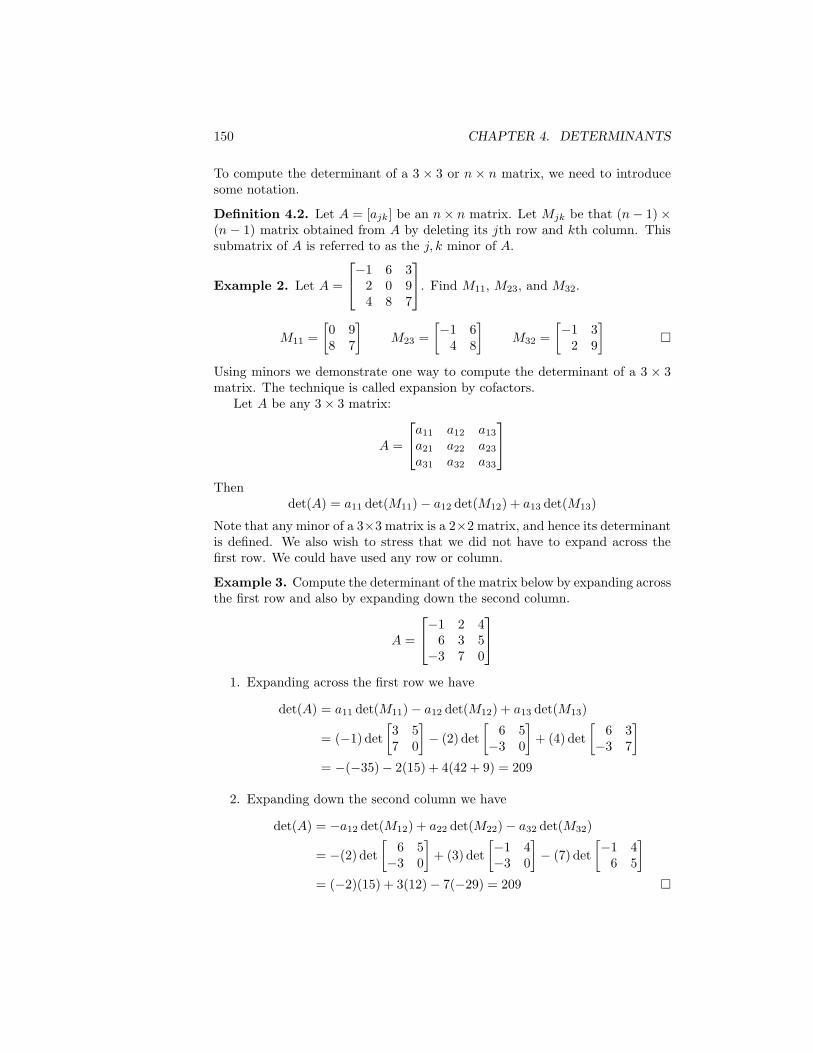
Definition 4.2. Let A = [ajk] be an n× n matrix. Let Mjk be that (n− 1)×(n − 1) matrix obtained from A by deleting its jth row and kth column. Thissubmatrix of A is referred to as the j, k minor of A.
Example 2. Let A =
−1 6 32 0 94 8 7
. Find M11, M23, and M32.
M11 =
[
0 98 7
]
M23 =
[
−1 64 8
]
M32 =
[
−1 32 9
]
�
Using minors we demonstrate one way to compute the determinant of a 3 × 3matrix. The technique is called expansion by cofactors.
Let A be any 3× 3 matrix:
A =
a11 a12 a13a21 a22 a23a31 a32 a33
Thendet(A) = a11 det(M11)− a12 det(M12) + a13 det(M13)
Note that any minor of a 3×3 matrix is a 2×2 matrix, and hence its determinantis defined. We also wish to stress that we did not have to expand across thefirst row. We could have used any row or column.
Example 3. Compute the determinant of the matrix below by expanding acrossthe first row and also by expanding down the second column.
A =
−1 2 46 3 5
−3 7 0
1. Expanding across the first row we have
det(A) = a11 det(M11)− a12 det(M12) + a13 det(M13)
= (−1) det
[
3 57 0
]
− (2) det
[
6 5−3 0
]
+ (4) det
[
6 3−3 7
]
= −(−35)− 2(15) + 4(42 + 9) = 209
2. Expanding down the second column we have
det(A) = −a12 det(M12) + a22 det(M22)− a32 det(M32)
= −(2) det
[
6 5−3 0
]
+ (3) det
[
−1 4−3 0
]
− (7) det
[
−1 46 5
]
= (−2)(15) + 3(12)− 7(−29) = 209 �

4.1. PROPERTIES OF THE DETERMINANT 151
It seems from the above two computations that minus signs creep in at random.That is not true. There is a rule for deciding whether or not a minus sign shouldappear, and it is given in the following theorem.
Theorem 4.1. Let A = [ajk] be any n× n matrix. Then
det(A) =
n∑
j=1
(−1)j+kajk det(Mjk) k = 1, 2 . . . , n
expansion down the kth column
(4.1)
det(A) =
n∑
k=1
(−1)j+kajk det(Mjk) j = 1, 2 . . . , n
expansion across the jth row
Figure 4.1 should clarify whether or not a minus sign precedes the term det(Mjk).Notice that the 1,1 entry has a + sign, and whenever we move one space hori-zontally or vertically the sign changes. Since it takes three moves to go from 1,1 to 2, 3, the coefficient of a23 in (4.1) equals − det(M23).
The terms (−1)j+k det(Mjk) are called the cofactors of ajk, hence the phraseexpansion by cofactors. Notice that this theorem reduces the problem of com-puting the determinant of an n × n matrix to the problem of calculating thedeterminant of an (n − 1) × (n − 1) matrix. Continued use of this procedurewill reduce the original problem to one of calculating the determinants of 2× 2matrices.
+ − + − + · · ·− + − + − · · ·+ −−+− + − + · · ·...
Figure 4.1
It is clear that computing the determinant of a matrix, especially a largeone, is painful. It’s also clear that the more zeros in a matrix the easier thechore. The following theorems enable us to increase the number of zeros in amatrix and at the same time keep track of how the value of the determinantchanges.
Theorem 4.2. Let A be a square matrix. If A1 is a matrix obtained from A byinterchanging any two rows or columns, then det(A1) = − det(A).
152 CHAPTER 4. DETERMINANTS
Example 4.
det
1 2 40 3 21 0 5
= − det
0 3 21 2 41 0 5
: rows one and two interchanged
det
1 2 40 3 21 0 5
= − det
1 4 20 2 31 5 0
: columns two and three interchanged
�
Corollary 4.1. If an n × n matrix has two identical rows or columns, itsdeterminant must equal zero.
Proof. The preceding theorem says that if you interchange any two rows orcolumns, the determinant changes sign. But if the two rows interchanged areidentical, the determinant must remain unchanged. Since zero is the only num-ber equal to its negative, we have det(A) = 0.
Example 5.
a. det
[
1 21 2
]
= 2− 2 = 0
b. det
1 −6 12 3 81 −6 1
= 0: rows one and three are identical �
Theorem 4.3. If any row or column of a square matrix A is multiplied by aconstant c to get a matrix A1, then det(A1) = c[det(A)].
Corollary 4.2. If a square matrix A has a row or column of zeros, thendet(A) = 0.
Example 6.
det
3 4 126 16 309 8 21
= det
3(1) 4 123(2) 16 303(3) 8 21
= 3det
1 4 122 16 303 8 21
= 3det
1 4 122(1) 2(8) 2(15)3 8 21
= 6det
1 4 3(4)1 8 3(5)3 8 3(7)
= 18 det
1 4(1) 41 4(2) 53 4(2) 7
= 72 det
1 1 41 2 53 2 7
�
4.1. PROPERTIES OF THE DETERMINANT 153
Theorem 4.4. If any multiple of a row (column) is added to another row (col-umn) of a square matrix A to get another matrix A1, then det(A1) = det(A).
Example 7.
det
1 1 41 2 53 2 7
= det
1 1 40 1 13 2 7
= det
1 1 40 1 10 −1 −5
= det
1 1 40 1 10 0 −4
= (1) det
[
1 10 −4
]
= −4 �
This last example illustrates perhaps the easiest way to evaluate the determinantof a matrix. That is, use the elementary row or column operations to get a rowor column with at most one nonzero entry and then use Theorem 4.1.
Our next example also demonstrates this idea. The reader might try com-puting the determinant in this example by using Theorem 4.1 directly and thencomparing the two techniques.
Example 8.
det
2 1 −1 01 1 0 40 0 1 −21 0 1 1
= det
2 1 −1 −21 1 0 40 0 1 01 0 1 3
= det
2 1 −21 1 41 0 3
= det
0 1 −80 1 11 0 3
= det
[
1 −81 1
]
= 9 �
Theorem 4.5. Let A and B be two n× n matrices. Then
det(AB) = det(A) det(B)
Example 9. Let A =
[
3 41 −2
]
, B =
[
1 3−2 8
]
. Verify Theorem 4.5 for these
two matrices.
Solution.
det(A) = det
[
3 41 −2
]
= −10 det(B) = det
[
1 3−2 8
]
= 14
det(AB) = det
[
−5 415 −13
]
= −140 = (−10)(14) = det(A) det(B) �
Theorem 4.6. Let A be any square matrix and let AT be its transpose, then
det(A) = det(AT )
154 CHAPTER 4. DETERMINANTS
Example 10. Verify Theorem 4.6 for the matrix A =
[
6 4−2 3
]
.
Solution.
det(A) = det
[
6 4−2 3
]
= 18− (−8) = 26
det(AT ) = det
[
6 −24 3
]
= 18− (−8) = 26 = det(A) �
Theorem 4.7. A square matrix A is invertible if and only if det(A) is nonzero.
This last theorem is one that we use repeatedly in the remainder of this text.For example, in the next section we discuss how to compute the inverse of amatrix in terms of the determinants of its minors, and in Chapter 5 we use anequivalent version of Theorem 4.7 that says, if ker(A) has nonzero vectors in it,then det(A) = 0.
Problem Set 4.1
1. Compute the determinants of each of the following matrices:
a.
[
−6 01 2
]
b.
[
−2 1−4 2
]
c.
1 2 34 6 2
−1 4 1
d.
−1 2 6 41 0 2 80 3 9 62 7 5 6
2. Compute the determinants of each of the following matrices:
a.
[
1 32 4
]
b.
[
1 23 4
]
c.
1 0 −24 6 01 1 0
d.
1 4 10 6 1
−2 0 0
3. a. det
1 2 34 5 67 8 9
b. det
a1 a2 a3a1 + k a2 + k a3 + ka1 + 2k a2 + 2k a3 + 2k
4. a. det
2 3 03 4 10 1 −2
b. det
1 0 20 −2 12 1 4
5. If E is an elementary row matrix associated with adding a multiple of onerow to another, then det(E) =?
6. Let A be any upper or lower triangular matrix., Show that det(A) =a11a22 . . . ann; that is, the determinant of A equals the product of thediagonal entries of A.
4.1. PROPERTIES OF THE DETERMINANT 155
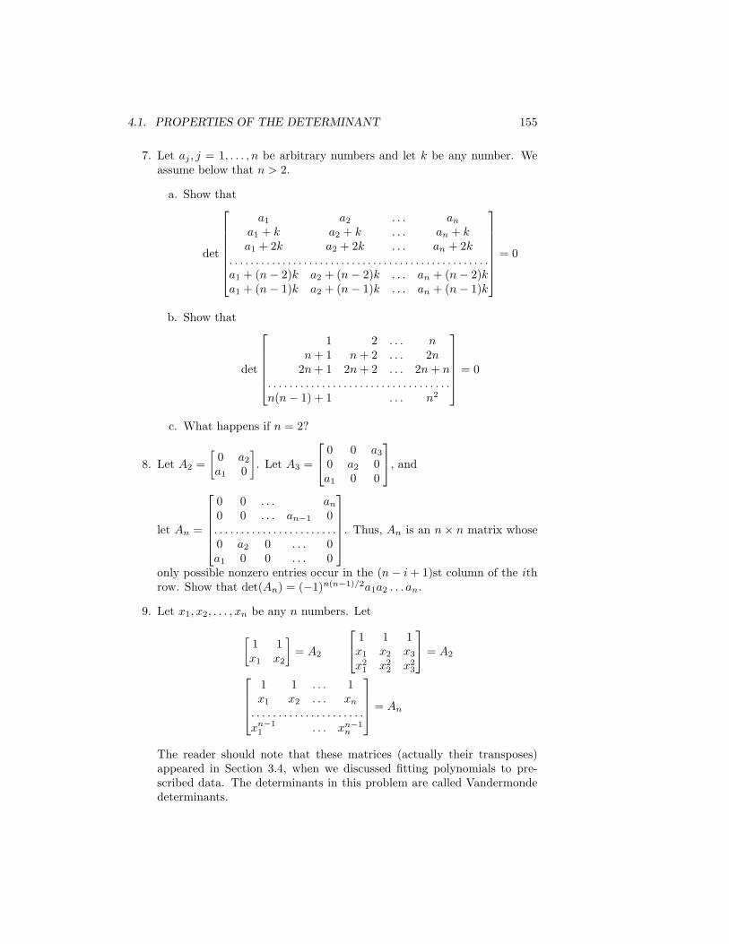
7. Let aj , j = 1, . . . , n be arbitrary numbers and let k be any number. Weassume below that n > 2.
a. Show that
det
a1 a2 . . . ana1 + k a2 + k . . . an + ka1 + 2k a2 + 2k . . . an + 2k
. . . . . . . . . . . . . . . . . . . . . . . . . . . . . . . . . . . . . . . . . . . . . . . . .a1 + (n− 2)k a2 + (n− 2)k . . . an + (n− 2)ka1 + (n− 1)k a2 + (n− 1)k . . . an + (n− 1)k
= 0
b. Show that
det
1 2 . . . nn+ 1 n+ 2 . . . 2n2n+ 1 2n+ 2 . . . 2n+ n
. . . . . . . . . . . . . . . . . . . . . . . . . . . . . . . . . .n(n− 1) + 1 . . . n2
= 0
c. What happens if n = 2?
8. Let A2 =
[
0 a2a1 0
]
. Let A3 =
0 0 a30 a2 0a1 0 0
, and
let An =
0 0 . . . an0 0 . . . an−1 0. . . . . . . . . . . . . . . . . . . . . . .0 a2 0 . . . 0a1 0 0 . . . 0
. Thus, An is an n× n matrix whose
only possible nonzero entries occur in the (n− i+ 1)st column of the ithrow. Show that det(An) = (−1)n(n−1)/2a1a2 . . . an.
9. Let x1, x2, . . . , xn be any n numbers. Let
[
1 1x1 x2
]
= A2
1 1 1x1 x2 x3x21 x22 x23
= A2
1 1 . . . 1x1 x2 . . . xn. . . . . . . . . . . . . . . . . . . . .xn−11 . . . xn−1
n
= An
The reader should note that these matrices (actually their transposes)appeared in Section 3.4, when we discussed fitting polynomials to pre-scribed data. The determinants in this problem are called Vandermondedeterminants.
156 CHAPTER 4. DETERMINANTS
a. Show that det(A2) = x2 − x1.
b. det(A3) = (x3 − x2)(x3 − x1)(x2 − x1).
c. Find a similar formula for det(An).
10. Let A be any n × n matrix. Show that det(A) equals zero if and only ifthe rows (columns) of A form a linearly dependent set of vectors in Rn.(Hint: Use Theorems 4.4 and 4.7.)
11. Let A be a nonsingular matrix. Show that det(A−1) = [det(A)]−1. (Hint:AA−1 = In. Now use Theorem 4.5.)
12. Let S be any scalar matrix, that is, S = cIn for some number c. Showthat det(S) = cn.
13. Let A and B be any two similar matrices; that is, there is a nonsingularmatrix P such that A = PBP−1. Show that det(A) = det(B).
14. Compute the determinants of the following matrices:
a.
2 3 4 53 4 5 64 5 6 75 6 7 8
b.
−8 7 6 −12 5 4 31 −5 7 110 2 −3 6
15. A matrix is said to be skew symmetric if A = −AT . Thus
[
0 −11 0
]
is
skew symmetric, while
[
0 11 0
]
is not.
a. Show that all the diagonal elements of a skew symmetric matrix areequal to zero.
b. Let A be a 3× 3 skew symmetric matrix. Show that det(A) = 0.
c. If A is a 2× 2 skew symmetric matrix, must det(A) = 0?
d. What happens if A is an n× n skew symmetric matrix?
16. Let P be an n× n permutation matrix. Show that det(P ) = ±1. For thedefinition of a permutation matrix see problem 13 in Problem Set 1.5.
4.2 The Adjoint Matrix and A−1
Theorem 4.7 states that A is invertible if and only if det(A) is nonzero. Inthis section we show how to compute the inverse of a matrix by using thedeterminants of its (n − 1) × (n − 1) minors (cf. Definition 4.2). Since thesedeterminants will appear quite frequently, we introduce a special notation forthem.

4.2. THE ADJOINT MATRIX AND A−1 157
Definition 4.3. Let A = [ajk] be any n × n matrix. The cofactor of ajk,denoted by Ajk, is defined to be
Ajk = (−1)j+k det(Mjk)
where Mjk is the j, k minor ofA.
Example 1. Let A =
−1 6 32 0 94 8 7
.
A11 = (−1)2(−72) A12 = (−1)3(14− 36) A13 = (−1)4(16)A21 = −(42− 24) A22 = (−7− 12) A23 = −(−8− 24)A31 = (54) A32 = −(−9− 6) A33 = (−12)
�
Using the cofactors of a matrix, we construct its adjoint matrix.
Definition 4.4. Let A = [ajk] be an n× n matrix. The adjoint matrix of A isthe following n× n matrix:
adj(A) = [Ajk]T
where Ajk are the cofactors of A.
Note that the transpose of the matrix [Ajk] must be taken.
Example 2. Let A =
−1 6 32 0 94 8 7
. From Example 1 and the definition of
adj(A) we have
adj(A) =
−72 22 16−18 −19 3254 15 −12
T
=
−72 −18 5422 −19 1516 32 −12
�
Example 3. Let A be the matrix in the preceding example. Compute det(A)and A[adj(A)].
det(A) = det
−1 6 32 0 94 8 7
= det
−1 6 30 12 150 32 19
= 252
A[adj(A)] =
−1 6 32 0 94 8 7
−72 −18 5422 −19 1516 32 −12
=
252 0 00 252 00 0 252
= 252I3 = det(A)I3 �
158 CHAPTER 4. DETERMINANTS
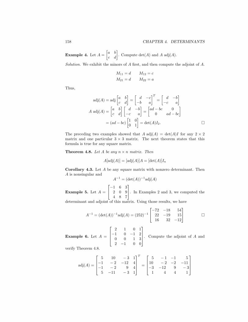
Example 4. Let A =
[
a bc d
]
. Compute det(A) and A adj(A).
Solution. We exhibit the minors of A first, and then compute the adjoint of A.
M11 = d M12 = c
M21 = d M22 = a
Thus,
adj(A) = adj
[
a bc d
]
=
[
d −c−b a
]T
=
[
d −b−c a
]
A adj(A) =
[
a bc d
] [
d −b−c a
]
=
[
ad− bc 00 ad− bc
]
= (ad− bc)
[
1 00 1
]
= det(A)I2. �
The preceding two examples showed that A adj(A) = det(A)I for any 2 × 2matrix and one particular 3 × 3 matrix. The next theorem states that thisformula is true for any square matrix.
Theorem 4.8. Let A be any n× n matrix. Then
A[adj(A)] = [adj(A)]A = [det(A)]In
Corollary 4.3. Let A be any square matrix with nonzero determinant. ThenA is nonsingular and
A−1 = (det(A))−1adj(A)
Example 5. Let A =
−1 6 32 0 94 8 7
. In Examples 2 and 3, we computed the
determinant and adjoint of this matrix. Using those results, we have
A−1 = (det(A))−1adj(A) = (252)−1
−72 −18 5422 −19 1516 32 −12
�
Example 6. Let A =
2 1 0 1−1 0 −1 20 0 1 32 −1 0 0
. Compute the adjoint of A and
verify Theorem 4.8.
adj(A) =
5 10 − 3 1−1 − 2 −12 4−1 − 2 9 45 −11 − 3 1
T
=
5 − 1 −1 510 − 2 −2 −11−3 −12 9 − 31 4 4 1
4.2. THE ADJOINT MATRIX AND A−1 159
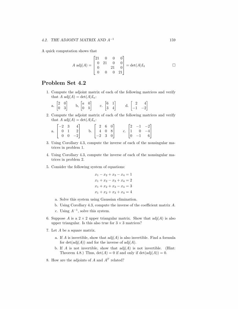
A quick computation shows that
A adj(A) =
21 0 0 00 21 0 00 21 00 0 0 21
= det(A)I4 �
Problem Set 4.2
1. Compute the adjoint matrix of each of the following matrices and verifythat A adj(A) = det(A)In:
a.
[
2 00 3
]
b,
[
a 00 b
]
c.
[
6 13 4
]
d.
[
2 4−1 −2
]
2. Compute the adjoint matrix of each of the following matrices and verifythat A adj(A) = det(A)In:
a.
−2 3 40 1 20 0 −2
b.
2 6 04 0 8
−2 3 0
c.
2 −1 −21 0 −40 −1 6
3. Using Corollary 4.3, compute the inverse of each of the nonsingular ma-trices in problem 1.
4. Using Corollary 4.3, compute the inverse of each of the nonsingular ma-trices in problem 2.
5. Consider the following system of equations:
x1 − x2 + x3 − x4 = 1
x1 + x2 − x3 + x4 = 2
x1 + x2 + x3 − x4 = 3
x1 + x2 + x3 + x4 = 4
a. Solve this system using Gaussian elimination.
b. Using Corollary 4.3, compute the inverse of the coefficient matrix A.
c. Using A−1, solve this system.
6. Suppose A is a 2 × 2 upper triangular matrix. Show that adj(A) is alsoupper triangular. Is this also true for 3× 3 matrices?
7. Let A be a square matrix.
a. If A is invertible, show that adj(A) is also invertible. Find a formulafor det(adj(A)) and for the inverse of adj(A).
b. If A is not invertible, show that adj(A) is not invertible. (Hint:Theorem 4.8.) Thus, det(A) = 0 if and only if det(adj(A)) = 0.
8. How are the adjoints of A and AT related?
160 CHAPTER 4. DETERMINANTS
4.3 Cramer’s Rule
Cramer’s rule is a formula for computing the solution to a system of linearequations when the coefficient matrix A is nonsingular. This formula is just thecomponent verseion of the equation
A−1 = (det(A))−1 adj(A) (4.2)
We derive Cramer’s rule for a system of two equations with two unknowns beforestating the rule for n equations with n unknowns.
Example 1. Find the solution to
a11x1 + a12x2 = b1
a21x1 + a22x2 = b2 (4.3)
Assuming that det(A) = a11a22 − a12a21 6= 0,
A−1 = (det(A))−1 adj(A) = (detA)−1
[
a22 −a22−a21 a11
]
Thus,[
x1x2
]
= A−1
[
b1b2
]
= (detA)−1
[
a22 −a22−a21 a11
] [
b1b2
]
and[
x1x2
]
=
[
b1a22 − b2a12b2a11 − b1a21
]
(detA)−1
Thus,
x1 =b1a22 − b2a12
det(A)=
det
[
b1 a12b2 a22
]
det(A)
x2 =b2a11 − b1a21
det(A)=
det
[
a11 b1a21 b2
]
det(A)�
Thus we see that x1 can be expressed as the ratio of two determinants. Thematrix in the numerator is obtained by replacing the first column of A withthe right-hand side of (4.3). To calculate x2, the matrix in the numerator isobtained by replacing the second column of A with the right-hand side of (4.3).
Consider the general system with n equations and n unknowns
Axxx = bbb (4.4)
where A = [ajk] is an n × n nonsingular matrix xxx = [x1, . . . , xn]T , and bbb =
[b1, . . . , bn]T . We know that
xxx = A−1bbb = (detA)−1 adj(A)bbb (4.5)

4.3. CRAMER’S RULE 161
Using (4.5), we write xk in terms of bbb:
xk = (detA)−1(A1kb1 +A2kb2 + · · ·+Ankbn) (4.6)
remember adj(A) = [Ajk]T , where Ajk is the cofactor of ajk. The last factor
in (4.6) can be thought of as the expansion by minors (going down the kthcolumn) of the determinant of the matrix obtained by replacing the kth columnof A with the column [b1, . . . , bn]
T . That is,
xk =
det
a11 . . . a1(k−1) b1 a1(k+1) . . . a1n. . . . . . . . . . . . . . . . . . . . . . . . . . . . . . . . . . . . . . . . . .aj1 . . . . . . . . . . . . bj . . . . . . . . . . . . ajn. . . . . . . . . . . . . . . . . . . . . . . . . . . . . . . . . . . . . . . . . .an1 . . . an(k−1) bn an(k+1) . . . ann
det(A)(4.7)
Formula (4.7) is Cramer’s rule. Note that it is valid only for systems whosecoefficient matrix is nonsingular.
Example 2. Find the value of x4 for which x1, x2, x3, x4, and x5 solves thefollowing system:
2x1 + x2 + 2x5 = 2x1 + x4 = 2
3x2 + x3 + 2x4 = −1x1 + x2 + x4 + x5 = −1
x3 + x4 + x5 = −1
An easy computation shows that the coefficient matrix A has a determinantequal to −7. Thus, A is nonsingular and we have
x4 =
det
2 1 0 2 21 0 0 2 00 3 1 −1 01 1 0 −1 10 0 1 −1 1
det(A)= −
(
13
7
)
�
We now have three techniques for solving systems of equations: Gaussian elimi-nation, which always works; inversion of the coefficient matrix A, i.e., computeA−1; and Cramer’s rule. The last two methods assume, of course, that A isinvertible. For small systems, n = 2, 3, or 4, any of these methods would befine, at least if A is invertible. For large n, however, the most efficient methodto use in solving a system of equations is usually Gaussian elimination. It isfor this reason that Cramer’s rule is a theoretical rather than a problem-solvingtool.
162 CHAPTER 4. DETERMINANTS
Problem Set 4.3
1. Use Cramer’s rule to solve each of the following systems of equations:
a. 2x1 + 2x2 = 7 b. −8x1 + 6x2 = 48x1 + x2 = −2 3x1 + 2x2 = 6
2. Use Gaussian elimination to solve each of the systems in problem 1.
3. Use Cramer’s rule to solve the following system:
2x1 − 6x2 + x3 = 2x2 + x3 = 1
x1 − x2 − x3 = 0
4. Consider the following system of equations:
2x1 + x2 + x3 − x4 = 13x1 − x2 + x3 + x4 = 0−x1 + x2 − x3 + x4 = 06x1 − x2 + x4 = 0
a. Use Cramer’s rule to solve for x1.
b. Use Gaussian elimination to solve for x1.
5. Consider the following system of equations:
−x1 + 3x2 + x3 = 7x1 − x2 − x3 = −2
−x1 + 6x2 + 2x3 = 3
a. Solve this systsem using Cramer’s rule.
b. Solve using Gaussian elimination.
c. Solve by finding the inverse of the coefficient matrix.
6. Solve the following system by using Cramer’s rule.
2x1 − x3 = 12x1 + 4x2 − x3 = 0x1 − 8x2 − 3x3 = −2
7. Solve using Cramers’ rule.
x1 + x2 + x3 = ax1 + (1 + a)x2 + x3 = 2ax1 + x2 + (1 + a)x3 = 0
8. Solve using Cramer’s rule.
x1 + x2 + x3 + x4 = 4x1 + 2x2 + 2x3 + 2x4 = 1x1 + x2 + 2x3 + 2x4 = 2x1 + x2 + x3 + 2x4 = 3

4.4. AREA AND VOLUME 163
4.4 Area and Volume
Given any two vectors in R2 that are not parallel, they determine a parallel-
ogram; cf. problems 9 and 10 in Section 2.1. With a few manipulations it ispossible to express the area of this parallelogram as the absolute values of thedeterminant of a matrix constructed from the coordinates of these vectors.
Example 1. Compute the area of the parallelogram determined by the vectors(1,2) and (8,0) (see Figure 4.2).
The area of this parallelogram is the base length 8 times the height 2.
Area = 8× 2 = det
[
8 10 2
]
(4.8)
where the columns of the matrix
[
8 10 2
]
are the coordinates of the two vectors
(8,0) and (1,2), with respect to the standard basis of R2. �
x1
(1,2)
(8,0)
x2
Figure 4.2
We derive a similar formula for any two vectors (a1, a2) and (b1, b2). Our proofand picture assume that both vectors lie in the first quadrant, but the othercases can be handled in a similar manner.
Consider the parallelogram determined by the two vectors (a1, a2) and (b1, b2)(see Figure 4.3).
Area of parallelogram OBCA = area of triangle(OBP2)
+ area of trapezoid(P2BCP3)
− area of triangle(OAP1)
− area of trapezoid(P1ACP3)
=1
2(b1b2) +
1
2(a1)(b2 + a2 + b2)
− 1
2(a1a2)−
1
2(b1)(a2 + a2 + b2)
= a1b2 − a2b1 = det
[
a1 b1a2 b2
]
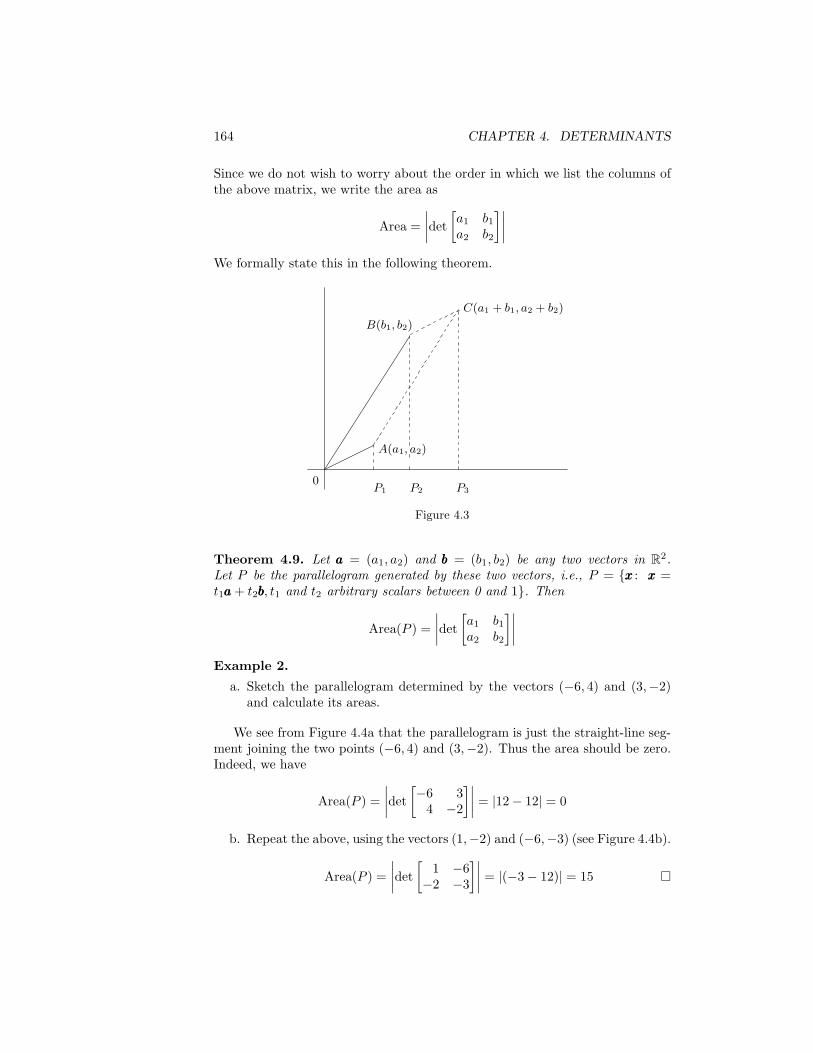
164 CHAPTER 4. DETERMINANTS
Since we do not wish to worry about the order in which we list the columns ofthe above matrix, we write the area as
Area =
∣
∣
∣
∣
det
[
a1 b1a2 b2
]∣
∣
∣
∣
We formally state this in the following theorem.
0P1 P2 P3
B(b1, b2)
C(a1 + b1, a2 + b2)
A(a1, a2)
Figure 4.3
Theorem 4.9. Let aaa = (a1, a2) and bbb = (b1, b2) be any two vectors in R2.Let P be the parallelogram generated by these two vectors, i.e., P = {xxx : xxx =t1aaa+ t2bbb, t1 and t2 arbitrary scalars between 0 and 1}. Then
Area(P ) =
∣
∣
∣
∣
det
[
a1 b1a2 b2
]∣
∣
∣
∣
Example 2.
a. Sketch the parallelogram determined by the vectors (−6, 4) and (3,−2)and calculate its areas.
We see from Figure 4.4a that the parallelogram is just the straight-line seg-ment joining the two points (−6, 4) and (3,−2). Thus the area should be zero.Indeed, we have
Area(P ) =
∣
∣
∣
∣
det
[
−6 34 −2
]∣
∣
∣
∣
= |12− 12| = 0
b. Repeat the above, using the vectors (1,−2) and (−6,−3) (see Figure 4.4b).
Area(P ) =
∣
∣
∣
∣
det
[
1 −6−2 −3
]∣
∣
∣
∣
= |(−3− 12)| = 15 �

4.4. AREA AND VOLUME 165
(3,−2)
(−6, 4)
(a)
(1,−2)
(b)
(−6,−3)
Figure 4.4
As one would expect, there is a generalization of this formula to higher dimen-sions, and we state it in the next theorem.
Theorem 4.10. Let {xxx1, . . . ,xxxn} be any n vectors in Rn. Let P be the n-dimensional parallelepiped generated by these vectors, that is,
P = {yyy : yyy = t1xxx1 + · · ·+ tnxxxn, 0 ≤ tj ≤ 1}Then the n-dimensional volume of P equals
Vol(P ) =
∣
∣
∣
∣
∣
∣
∣
∣
det
xxx1 xxx2 . . . xxxn...
......
......
...
∣
∣
∣
∣
∣
∣
∣
∣
(4.9)
The matrix in (4.9) is obtained by using the coordinates of the vector xxxj (withrespect to the standard basis) as the jth column. Thus, if we had the four
166 CHAPTER 4. DETERMINANTS
vectors
xxx1 = (1, 1, 2, 1) xxx2 = (−1,−1, 3, 4) xxx3 = (8, 9, 1, 1) xxx4 = (10, 11, 1, 0)
then the matrix would be
1 −1 8 101 −1 9 112 3 1 11 4 1 0
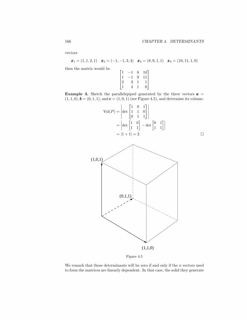
Example 3. Sketch the parallelepiped generated by the three vectors aaa =(1, 1, 0), bbb = (0, 1, 1), and ccc = (1, 0, 1) (see Figure 4.5), and determine its volume.
Vol(P ) =
∣
∣
∣
∣
∣
∣
det
1 0 11 1 00 1 1
∣
∣
∣
∣
∣
∣
=
∣
∣
∣
∣
det
[
1 01 1
]
− det
[
0 11 1
]∣
∣
∣
∣
= |1 + 1| = 2 �
(1,0,1)
(1,1,0)
(0,1,1)
Figure 4.5
We remark that these determinants will be zero if and only if the n vectors usedto form the matrices are linearly dependent. In that case, the solid they generate

4.4. AREA AND VOLUME 167
will lie in an (n − 1)-dimensional plane, and hence should have n-dimensionalvolume equal to zero. See Example 2a.
If L is a linear transformation from R2 to R2, it has a matrix representationA, where
A =
[
a11 a12a21 a22
]
As we saw in Chapter 3, L(eee1) = (a11, a21) and L(eee2) = (a12, a22). Thus,geometrically we can picture L as transforming the parallelogram generatedby eee1 and eee2 into the parallelogram generated by (a11, a21) and (a12, a22) (seeFigure 4.6). Moreover, we have
Area(L(P )) =
∣
∣
∣
∣
det
[
a11 a12a21 a22
]∣
∣
∣
∣
= | det(A)|
Since in this particular case we have area(P ) = 1, we may rewrite this formulaas
Area(L(P )) = | det(A)|area(P )
To see that this formula is true in general let xxx = (x1, x2) and yyy = (y1, y2). LetP be the parallelogram generated by xxx and yyy, that is,
P = {t1xxx+ t2yyy : 0 ≤ t1 ≤ 1, 0 ≤ t2 ≤ 1}
L[e1]
e2
L[e2]
e1
L[P ]
P
Figure 4.6
Then
L(P ) = {t1L(xxx) + t2L(yyy) : 0 ≤ t1 ≤ 1, 0 ≤ t2 ≤ 1}
where
L(xxx) = (a11x1 + a12x2, a21x1 + a22x2)
and
L(yyy) = (a11y1 + a12y2, a21y1 + a22y2).

168 CHAPTER 4. DETERMINANTS
We have from (4.9) that
Area(L(P )) =
∣
∣
∣
∣
det
[
a11x1 + a12x2 a11y1 + a12y2a21x1 + a22x2 a21y1 + a22y2
]∣
∣
∣
∣
=
∣
∣
∣
∣
det
([
a11 a12a21 a22
] [
x1 y1x2 y2
])∣
∣
∣
∣
=
∣
∣
∣
∣
det
[
a11 a12a21 a22
]
det
[
x1 y1x2 y2
]∣
∣
∣
∣
= | det(A)|[area(P )]
Thus, a linear transformation from R2 to R
2 maps parallelograms into parallel-ograms (rank A = 2), or line segments (rank A = 1), or a point (rank A = 0).Moreover, the change in area depends only on the linear transformation and noton the particular parallelogram. Naturally there is a generalization of this tohigher dimensions which we state below.
Theorem 4.11. Let A be the n×n matrix representation of L : Rn → Rn, withrespect to the standard basis of Rn. Let P be an n-dimensional parallelogramgenerated by the n vectors {xxx1, . . . ,xxxn}. Then L(P ) is generated by the n vectors{L(xxx1), . . . , L(xxxn)} and their volumes are related by the formula
Vol(L(P )) = | det(A)|Vol(P ) (4.10)
Problem Set 4.4
1. Calculate the area of the triangles whose vertices are:
a. (0,0), (1,6), (−2, 3) b. (8,17), (9,2), (4,6)
2. Calculate the volume of the tetrahedron whose vertices are:
a. (0,0,0), (1,−1, 2), (−3, 6, 7), (1,1,1)
b. (1,1,1), (−1,−1,−1), (0,4,8), (−3, 0, 2)
3. Find the area of the parallelograms determined by the following vectors;cf. problem 1.
a. (1,6), (−2, 3) b. (1,−15), (−4,−11)
4. Sketch the parallelograms P generated by the following pairs of vectors.Let O be the parallelogram generated by the standard basis vectors. Foreach of the parallelograms P find a linear transformation L such thatP = L(O).
a. (1,0), (1,2) b. (1,−1), (3,6)

4.4. AREA AND VOLUME 169
5. In R2, show that the straight line passing through the two points (a1, a2)and (b1, b2) has equation
det
x1 x2 1a1 a2 1b1 b2 1
= 0
6. Let L, a linear transformation from R2 to R2, have matrix representation
A =
[
1 2−1 −2
]
Let P be the parallelogram generated by the vectors (−1, 2) and (1,3).Sketch P and L(P ) and compute their areas. Then verify (4.10).
7. Let A =
[
−1 −2−2 1
]
be the matrix representation of a linear transformation
L. Let P be the parallelogram generated by the following pairs of vectors:
a. (1,0), (0,1)
b. (1,1), (−1, 1)
In each case sketch P,L(P ), and verify (4.10).
8. Let A =
1 0 2−2 1 10 1 0
be the matrix representation of a linear transfor-
mation L. Let P be the solid generated by the following vectors:
a. (1,0,0), (0,1,0), (0,0,1)
b. (1,1,0), (1,0,1), (0,1,1)
In each case sketch P,L(P ), and verify (4.10).
Supplementary Problems
1. Let A = [ajk] be an n× n matrix. Define each of the following:
a. Mjk minor of A
b. Cofactor of ajk
c. Adj(A)
2. Compute the determinant and adjoint of each of the following matrices:
a.
[
3 42 5
] [
4 26 3
]
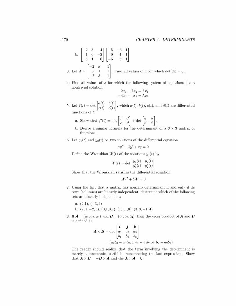
170 CHAPTER 4. DETERMINANTS
b.
−2 3 41 0 −25 1 6
5 −3 10 1 1
−5 5 1
3. Let A =
−2 x 1x 1 12 3 −1
. Find all values of x for which det(A) = 0.
4. Find all values of λ for which the following system of equations has anontrivial solution:
2x1 − 7x2 = λx1−4x1 + x2 = λx2
5. Let f(t) = det
[
a(t) b(t)c(t) d(t)
]
, which a(t), b(t), c(t), and d(t) are differential
functions of t.
a. Show that f ′(t) = det
[
a′ b′
c d
]
+ det
[
a bc′ d′
]
.
b. Derive a similar formula for the determinant of a 3 × 3 matrix offunctions.
6. Let y1(t) and y2(t) be two solutions of the differential equation
ay′′ + by′ + cy = 0
Define the Wronskian W (t) of the solutions yj(t) by
W (t) = det
[
y1(t) y2(t)y′1(t) y′2(t)
]
Show that the Wronskian satisfies the differential equation
aW ′ + bW = 0
7. Using the fact that a matrix has nonzero determinant if and only if itsrows (columns) are linearly independent, determine which of the followingsets are linearly independent:
a. (2,1), (−3, 4)
b. (2, 1,−2, 3), (0,1,0,1), (1,1,1,0), (3, 3,−1, 4)
8. If AAA = (a1, a2, a3) and BBB = (b1, b2, b3), then the cross product of AAA and BBBis defined as
AAA×BBB = det
iii jjj kkka1 a2 a3b1 b2 b3
= (a2b3 − a3b2, a3b1 − a1b3, a1b2 − a2b1)
The reader should realize that the term involving the determinant ismerely a mnemonic, useful in remembering the last expression. Showthat AAA×BBB = −BBB ×AAA and the AAA×AAA = 000.

4.4. AREA AND VOLUME 171
9. Verify the following formulas:
a. det
a b 0c d 00 0 e
= det
[
a bc d
]
e
b. det
a b 0 0c d 0 00 0 e f0 0 g h
= det
[
a bc d
]
det
[
e fg h
]
10. Let A =
[
A1 00 A2
]
be an n×n matrix, where A1 is an m×m matrix and
A2 is an (n−m)× (n−m) matrix, 1 ≤ m ≤ n− 1. Show that
det(A) = det(A1) det(A2)
11. A group (G , ·) is a mathematical system that consists of a collection ofobjects G and an operation · between two elements of G , which gives anelement of G . Thus, if x and y are elements of G , then x · y (we drop thedot in the future) is also in G . We also suppose that this operation, calledmultiplication, satisfies the following properties:
1. (xy)z = x(yz).
2. There is an identity element e in G such that ex = xe = xfor every x in G .
3. For each x in G , there is an x−1 in G such that xx−1 =x−1x = e
a. Show that the set of vectors in a vector space forms a group, thegroup operation being vector addition.
b. Let GL(n) denote the set of invertible n×n matrices, with the groupoperation being matrix multiplication. Show that GL(n) forms agroup. This group is called the general linear group of order n.
c. Let SL(n) denote the set of invertible n×nmatrices with determinantequal to 1. Show that SL(n), with the group operation being matrixmultiplication, is a group. This group is called the special lineargroup of order n.
d. Show that the set of all n × n matrices under matrix multiplicationdoes not form a group.
12. An n× n matrix P is said to be orthogonal if P−1 = PT .
a. Show that if P is orthogonal, then det(P ) = ±1.
b. Deduce from part a that if P is orthogonal and if K is some n-dimensional parallelepiped, then vol(PK) = vol(K).
172 CHAPTER 4. DETERMINANTS
c. Find a 2 × 2 matrix P that is not orthogonal, and for which det(P )equals 1.
d. Show that O(n), the set of n×n orthogonal matrices, forms a groupunder the operation of matrix multiplication; cf. problem 11.
13. A matrix B is said to be similar to the matrix A if there is a nonsingularmatrix P such that B = PAP−1.
a. Show that if B is similar to A, then det(B) = det(A).
b. Find a pair of 2 × 2 matrices A and B for which det(A) = det(B)and B is not similar to A. Hint: If B is similar to a scalar matrix,then B = A.
14. Find two 2×2 matrices A and B for which det(A+B) 6= det(A)+det(B).