Hydroinformatics and its applications at Delft Hydraulics

Hydroinformatics and its applications at Delft Hydraulics

Arthur E. Mynett

Arthur E. MynettDepartment of Strategic Research and

Development,Delft Hydraulics, Postbus 177,Rotterdamseweg 185, 2600 MH Delft,The Netherlands

ABSTRACT

Hydroinformatics concerns applications of advanced information technologies in the fields

of hydro-sciences and engineering. The rapid advancement and indeed the very success of

hydroinformatics is directly associated with these applications. The aim of this paper is to provide

an overview of some recent advances and to illustrate the practical implications of hydroinformatics

technologies. A selection of characteristic examples on various topics is presented here,

demonstrating the practical use at Delft Hydraulics. Most surely they will be elaborated

upon in a more detailed way in forthcoming issues of this Journal.

First, a very brief historical background is outlined to characterise the emergence and evolution

of hydroinformatics in hydraulic and environmental engineering practice. Recent advances in

computational hydraulics are discussed next. Numerical methods are outlined whose main

advantages lie in their efficiency and applicability to a very wide range of practical problems. The

numerical scheme has to adhere only to the velocity Courant number and is based upon a staggered

grid arrangement. Therefore the method is efficient for most free surface flows, including complex

networks of rivers and canals, as well as overland flows. Examples are presented for dam break

problems and inundation of polders. The latter results are presented within the setting of a

Geographical Information System.

In general, computational modelling can be viewed as a class of techniques very much based

on, and indeed quite well described by, mathematical equations. These equations often symbolically

represent underlying physical phenomena, like conservation of mass, momentum and energy.

Diversification to application areas where no clear mathematical formulation may (yet) be present

but where adequate data sets are available is illustrated by several practical examples. Again, using

computer based technologies, various applications of so-called sub-symbolic techniques like Artificial

Neural Networks (ANNs) are discussed and presented. Finally, some reflections on forthcoming

developments and likely implications for engineering practice as well as education are outlined.

Key words | Delft Hydraulics, computational hydraulics, dam break problems, inundation of polders,

artificial neural networks, Kohonen networks

INTRODUCTION AND HISTORIC BACKGROUND

Hydroinformatics is all about applications. Backed by

substantial theoretical considerations (Abbott 1991, 1993,

1994) the main emphasis has been on practical implemen-

tations of advanced information technologies in a wide

variety fields on hydrosciences and engineering (Babovic

1996). The rapid advancement and indeed the very success

of hydroinformatics is directly associated with such appli-

cations. Technological institutes and university research

groups have developed a wide range of hydroinformatics

technologies and demonstrated their relevance for practi-

cal situations in numerous engineering and consultancy

projects. This is clearly reflected by the increasing number

of contributions in the proceedings of the biennial

Hydroinformatics Conferences in Delft 1994, Zurich 1996

and Copenhagen 1998 (Verwey et al. 1994; Muller 1996;

Babovic & Larsen 1998).

83 © IWA Publishing 1999 Journal of Hydroinformatics | 01.2 | 1999

Yet another implication of the advancing field of

hydroinformatics is its role in education. Already in the

early 1990s, the International Institute for Infrastructural,

Hydraulic and Environmental Engineering (IHE Delft)

initiated a graduate course in hydroinformatics. Well over

100 professionals have been trained at both M.Sc. and

Ph.D. level. More recently, other universities worldwide

have established hydroinformatics branches or even

hydroinformatics departments. Within the European

Graduate School of Hydraulics short courses and summer

courses on hydroinformatics are being provided as well.

The International Association for Hydraulic Research

(IAHR) from the very beginning provided a constructive

platform for communication and exchange among univer-

sity research groups and technological institutes alike. A

special Section on Hydroinformatics was created, contrib-

uting to the biennial IAHR Conferences as well as initiat-

ing the intermittent series of biennial Hydroinformatics

Conferences mentioned above. Its origin and emphasis

notably lies within the European communities, but inter-

est and involvement from Asia and North America are

rapidly increasing. It may be worthwhile to note that the

next Hydroinformatics 2000 Conference will be held at

the renowned Iowa Institute of Hydraulics, USA.

Contacts with the International Association on Water

Quality (IAWQ) increased the awareness and necessity to

stimulate the introduction of hydroinformatics tech-

nologies in the field of practitioners. This clearly demon-

strates the growing interest and rapid development over

the past decade. The newly established joint IAHR/IAWQ

Journal of Hydroinformatics is the result of the mutual

interest of both organisations aiming to reach both

researchers and practitioners, hence stimulating further

advances of hydroinformatics applications in the next

millennium.

ADVANCES IN COMPUTATIONALHYDRAULICS MODELLING

The field of hydraulics deals with flow and transport

phenomena in both natural water systems (rivers,

estuaries) as well as in man-made systems (canals, pipes).

Hydraulics has a long tradition of providing a scientific

basis for engineering applications (Rouse 1950; Ippen

1966). At the time, quite often empirical relations obtained

from field observations or model scale experiments

provided the basis for constructing conceptual models.

Mathematics started playing an important role not only to

describe these empirical relations, but also to construct

analytical solutions to schematised model situations that

captured the essential features of particular phenomena.

Applying these techniques to help solve practical prob-

lems, however, quite often was very much a form of art

rather than science.

With the advent of rapidly increasing computer tech-

nology, digital processing and numerical techniques

became of interest as well. In the early 1970s an IAHR

working group was initiated ‘to investigate the role of

computers in hydraulic engineering’. Some could not

imagine that computers would add to or be useful for

anything else than fast and automated data collection and

data processing from model scale experiments. Others

started using computers to solve mathematical equations

numerically that could not be handled analytically. This

approach is often referred to as computational hydraulics.

In fact, nowadays, computational techniques are com-

monly applied in a wide range of fields in science and

engineering, ranging from physics to chemistry and

biology.

Of course, the first applications in computational

hydraulics concerned programming analytical formulae

rather than deriving generic numerical schemes and tech-

niques based on physical principles like conservation laws

for mass and momentum. And still, in particular in one-

dimensional flow modelling, considerable a priori knowl-

edge is required to provide the proper input, even for

commercially available packages. Concepts like ‘convey-

ance width’ for momentum conservation and ‘storage

width’ for mass conservation are just typical examples.

Hence, deciding on the proper choice of values for the

various coefficients associated with such systems often

requires considerable craftsmanship and experience.

Recent developments, however, extend the field of

computational hydraulics to multidimensional modelling

of complicated flow phenomena in arbitrarily shaped

geometries. More general, in the field of computational

fluid dynamics, research and applications are oriented

84 Arthur E. Mynett | Hydroinformatics at Delft Hydraulics Journal of Hydroinformatics | 01.2 | 1999

towards simulating time-varying multidimensional trans-

port processes in high Reynolds number turbulent

flow fields, using high performance vector and parallel

computers. One such example related to recent advances

in the field of computational hydraulics and presented

below, is taken from Stelling et al. (1998).

Numerical schemes for shallow-water flow modelling

Shallow-water flow problems are wide ranging, varying

from ocean dynamics, through estuaries up to inland

waters with rapidly varied flows, or artificial lakes with

dams that might break. The numerical techniques for

coastal regions and estuaries are often based upon very

efficient ADI methods (see, for example, Leendertse 1967),

or semi-implicit methods (see, for example, Casulli 1990).

The efficiency of these approaches is due to an implicit

time integration combined with the application of

‘staggered grids’. Despite their efficiency, these methods

are not very effective for flows with large gradients in the

water levels because of the presence of hydraulic jumps or

the occurrence of bores as a result of dam breaks.

A very different class of numerical techniques is

applied for rapid flows with hydraulic jumps and dam

break problems. These techniques are often based upon

non-staggered grids and the so-called ‘Godunov methods’

as developed for aerodynamics (for extensive overviews

see, for example, Hirsch (1990) or Toro (1997)). Appli-

cations of these techniques to shallow-water flow prob-

lems are described by Chaudry (1993) or Alcrudo &

Garcia-Navarro (1993).

Examples of large gradients are tidal bores or the

inundation of low lands, such as, in The Netherlands,

because of dike breaks. The drying and flooding of tidal

flats can also be considered locally as rapid varying flow.

Locally, tidal bores could occur and it is questionable

whether ‘flooding procedures’ as described by Stelling

et al. (1986) or Falconer & Chen (1991) give accurate

simulations of the local flooding.

To try to bridge the gap between the different

approaches, Stelling proposed a numerical technique that

in essence is based upon the classical staggered grids

and implicit integration schemes such as described

by Leendertse (1967) and Casulli (1990), but that can

be applied to problems that include large gradients.

This new scheme is based upon the following charac-

teristics:

1. The continuity equation is approximated such that

(i) mass is conserved not only globally but also

locally and (ii) the total water depth is guaranteed

to be always positive which excludes the necessity

of ‘flooding and drying’ procedures.

2. The momentum equation is approximated such that

a proper momentum balance is fulfilled near large

gradients.

The combination of positivity of water depths and mass

conservation assures a stable numerical solution. A proper

momentum balance provides that this stable solution con-

verges. The numerical principles and numerical examples

for flows with large gradients are explained in detail by

Stelling et al. (1998). The principles can be explained by

considering the following one dimensional unsteady flow

equations

∂z∂t+

∂(uh)∂x

= 0; (2.1a)

∂u∂t+ u

∂u∂x+ g

∂z∂x+ g

u|u|C2h

= 0, (2.1b)

where

u = velocity,

z = water level above plane of reference,

C = Chezy coefficient,

d = depth below plane of reference,

h = total water depth, h = z + d.

If the bottom is assumed not to be time varying, it follows

that the continuity equations can be rewritten as:

∂h∂t+

∂(uh)∂x

= 0, (2.2)

which can be considered a transport equation of the scalar

quantity h, allowing application of so-called positive

and monotone schemes (see Hirsch 1991). A simple

semi-discretization on a C-type staggered computational

grid as indicated below, leads to


dhdt+ (uh(u))0x = 0, at (i) at (i) (2.3a)

dudt+ a(u,u)+ gz0x + g

_u_uC2h(u)

= 0, at (i + Y) (2.3b)

The relation between the variables in a staggered grid

arrangement are indicated by (2.4),

↑ ↑z z

u h= z+ d u h= z+ d u (2.4)d d↓ ↓

i − Y i i + Y i + 1 i + 1Y

where hi refers to the water depth h at i, a(u,u) denotes

some advection approximation, and

(ui)0x =ui+Y − ui−Y

∆x,(zi+Y)0x =

zi+1 − zi∆x

(2.5)

hi+Y(u) = { hi, u>0hi + 1, u≤0

For discrete time integration there are numerous possi-

bilities (see, for example, Lambert 1991). A well-known

integration scheme is based upon the so-called theta

method, which does not require iterations for the solution

of nonlinear equations. Application to the conservation

equations leads to

hn+1 − hn

∆t+ (un+Ohn(un))0x = 0, at (i) (2.6a)

un+1 − un

∆t+ a(un,un)+ gz0x

n+O

+ gZun_un+1

C2hn= 0, at (i + Y), (2.6b)

where, un+O = Oun+1+ (1 − O)un, and zn+O is defined

accordingly. Stelling et al. (1998) also derived conditions

for strict positivity which can be ensured if

∆t·ui+Yn+O

∆x<1. (2.7)

Similar conditions can be derived for other flow direc-

tions. Simply fulfilling eq. (6) will prevent wet points from

drying, i.e. no special drying and flooding procedures are

required for this approach. It should be noted that the

description of the continuity equation in primitive vari-

ables rather than integrated quantities, has important

advantages: (i) it enables strict positive waterlevels,

and (ii) upwinding yields artificial viscosity without

influencing strict local mass conservation.

For sufficiently smooth solutions, advection approxi-

mations could well be based upon at least second order

local truncations errors. In that case numerical viscosity is

minimal. However, near local discontinuities in the sol-

ution, following from, for example, sharp bottom gradients

or hydraulic jumps, the ‘order of accuracy’ concept is

meaningless. Conservation properties are more important

aspects in such situations. In accordance with well-known

concepts from classical hydraulics, the following quan-

tities are considered: (i) mass, (ii) momentum and (iii)

energy head. The numerical approximations introduced

above are already mass conservative. For the advection

approximation only energy head and momentum are

considered. The so-called energy-head conserving

formulation of (2.1b) is given by

∂u∂t+

∂∂x

( Yu2+ gz)+ gu_u_

C2h= 0 (2.8)

while the momentum conserving formulation is expressed

by

∂∂t

(hu)+∂∂x

(hu2)+ gh∂z∂x+ gu_u_

C2h= 0. (2.9)

Both formulations (2.8) and (2.9) are completely equiva-

lent for continuous and sufficiently smooth solutions. At

local discontinuities, however, these equations have no

unique solution in general. Local discontinuities can

either be due to discontinuities in the bathymetry or due to

the nonlinearly of the equations such as near bores gener-

ated in dam break problems, or near hydraulic jumps. At

the discontinuity additional equations are needed to con-

nect the equations at both sides of the discontinuity. In

general, conservation of mass and momentum provides

the internal boundary conditions, although in case of

converging flows and steep bottom gradients conservation

of energy head can be applied as well, (see, for example,

Chaudry 1993).


For numerical approximation, conservation proper-

ties near large local gradients are again important. Near

steep bottom gradients mass conservation seems to be

imperative. Steep bottom gradients are quite common in

estuaries near tidal channels or near tidal flats. ‘Steepness’

is also a notion that depends on the local grid size. As the

grid size is smaller the local gradients become larger in

the sense that only few grid points are used for its rep-

resentation. Stelling et al. (1998) show two first-order

advection approximations, that can be applied for the

approximation of the advective terms of (2.8) or (2.9) and

that are either energy head or momentum conservative.

Under the assumption of a constant density, hydrostatic

pressure and no velocity gradient in vertical direction the

numerical approximation of the elementary mechanical

conservation law applied to a control volume of water

leads to

change of momentum transport of momentum

F∆xrd

dtSu

2(h+Y+ h−Y)DG+ Fq+1+ q

2ru −

q + q−1

2ru−1G

(2.10)

integrated hydrostatic pressure

+ Fgrh+Y+ h−Y

2(s+Y − s−Y)G = 0

where r denotes the constant density. The integrated

normal pressure follows from the assumption that in a

control volume, the hydrostatic pressure is assumed to be

given by:

p(x,z) = rg(z(x) − z), z(x) =xi + 1 − x

∆xzi +

x − xi∆x

zi+1. (2.11)

The integrated result of the normalised pressure now does

not depend upon the shape of the bottom profile. The only

assumption now is the linear distribution or the free

surface. It should be noted that many authors split the

pressure term into a gradient of the water depth and of the

bottom slope (see, for example, Chaudry 1993), as follows:

gh∂z∂x

= gh∂∂x

(h − d) =∂∂x

( Ygh2) − gh∂d∂x

. (2.12)

This formulation follows from mathematical manipulation

and does not necessarily represent a proper momentum

balance in case of discontinuous steps in the bottom

profile ∂d/∂x where might tend to infinity. In this way

so-called flux splitting methods can be applied, but the

shape of the bottom profile now becomes important for a

numerical approximation. From a physical point of view

this is wrong. Of course both approaches can lead to

consistent approximations: i.e. for sufficiently smooth

solutions the differences are minor and only near discon-

tinuities differences might play an important role. In the

formulation by Stelling et al. (1998) all possibilities are

included, so that energy head conservation can be chosen

for converging flows and momentum conservation for

diverging flows.

According to some authors (see Toro 1997), energy

head conservation is to be used only if solutions are

smooth. For proper shock speeds and shock locations it is

imperative to apply a proper momentum balance. How-

ever, discontinuities sometimes are not only due to shock

formation but also due to the bathymetry. In that case (see

Chaudry 1993), sometimes energy head conservation is a

better assumption for converging flow. For example, rating

curves for sluice gates can be derived from the assumption

of energy head conservation in the upstream part, contrac-

tion in the sluice gate and momentum conservation

in the down stream part of the sluice gate. Of course it is

possible at al times, to impose momentum conservation

throughout.

Integration in time can be based upon various time

integration methods, e.g. the implicit midpoint rule (see

Lambert 1991). Strict application for O = Y will not destroyany of the conservation properties. The equations, how-

ever, are then nonlinear. This necessitates the application

of iterative solvers. By local linearization, iteration can be

avoided. Strict conservation is then difficult to prove.

Practical experience has shown, however, that the differ-

ences are small. To minimise the amount of computational

effort, an implicit approach has been applied. The implicit

equations are symmetric and positive definite and can be

solved by CG methods (see, for example, Casulli 1990).

The principles explained here can be applied, with-

out any alteration, to more general one-dimensional

equations including general cross-sections and they can be

extended to two-dimensional flow equations describing

the simulation of flow over dry land. Some applications

are presented below.


Application to dam break problems

One such example presented here is related to a two-

dimensional dam break problem. As a schematisation the

domain is considered to be rectangular and consisting of

64 × 114 grid points, the grid size corresponding to

∆x = 1 m. The upper reach has an initial water level

h0 = 5 m. The lower reach has an initial water level

h1 = 0 m, i.e. a dry bed. Figure 1 shows the water levels

after 5 seconds for downstream dry bed conditions. To

demonstrate the effect of the downstream boundary con-

dition, Figure 2 shows the results for a wet bed condition,

again after 5 seconds. The shape of the wavefront is seen

to be quite different.

In fact, these features correspond to the correct physi-

cal behaviour as observed in experiments and can be

verified using local analytical solutions. It should be

noted, however, that only very few numerical schemes are

able to represent the quite different behaviour in both

situations. Quite often only wet bed downstream con-

ditions are considered, which indeed is relevant in case of

a reservoir dambreak in a river. However, in case of

inundation of polders due to dike break, dry bed con-

ditions should be considered for overland flow. Apart

form the specific form of the wavefront, the speed of

propagation is quite different in either situation. The

numerical scheme developed by Stelling et al. (1998) is

capable of representing both conditions within the same

simulation. Hence it is particularly useful for – and in fact

the only way for proper modelling of – solving practical

problems related to the inundation of polders.

Application to inundation of polders

The method introduced above provides the basic compu-

tational kernel for the DELFT-FLS system, the numerical

flooding simulation package developed by Delft Hydraul-

ics. The DELFT-FLS system is a two-dimensional hydro-

dynamic simulation package especially suited to simulate

the dynamic behaviour of overland flow over initially dry

land. It is based on the full two-dimensional shallow water

equations. These equations are solved following the finite-

difference numerical technique described above on a

rectangular staggered grid. The technique always guaran-

tees a positive water depth, and allows flow computations

on initially dry land without using any special drying/

wetting procedure. It allows a sound simulation of sub- and

supercritical flows. It gives accurate and stable results dur-

ing flow computations on very steep slopes, such as dike

walls, structures, etc. It provides realistic and reliable pre-

dictions of floods due to dike or dam break, dike over-

toping, coast over-toping, heavy rainfalls and other natural

hazards.

DELFT-FLS is equipped with an automatic time-step

estimator which reduces or enlarges the computational

time-step according to the flow characteristics at any

moment of the simulation. The package requires good

topographical data. It can be given as a GIS-layer (GIS:

Geographical Information System) or manually on a suit-

able rectangular grid. The levels and positions of roads,

levees and other infrastructure are also required. A land use

map (or a similar representation) is also necessary. The

‘land use’ can easily be converted to hydraulic roughness

coefficients, since it is provided with experience based

ecotype roughness relationships. Internal boundary con-

ditions are included to simulate dam break/dike break

events.

Figure 1 | Two-dimensional dam break, dry bed conditions.

Figure 2 | Two-dimensional dam break, wet bed conditions.


The possible outputs are water levels, water depths,

velocities (magnitude and velocity fields), current

lines, inundation depth class intervals. These results

can be given in GIS format for presentation and further

post-processing. The presentation of results using other

packages is also possible.

Simulation of flooding in a GIS-environment

An example is presented here for a typical lowland

situation. The polders of Tiel and Culemborg in The

Netherlands are limited by the rivers Lek on the North

and Waal on the South (both Rhine branches), by the

Amsterdam–Rhine channel on the East and by other

channels and dikes on the west. The region has been

schematised within a rectangular grid with 42,000 active

cells (Kernkamp & de Jonge 1997). The size of each cell

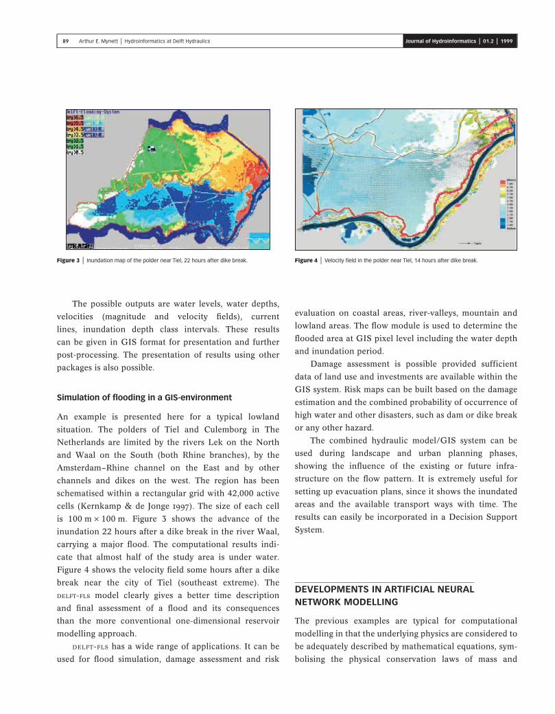
is 100 m × 100 m. Figure 3 shows the advance of the

inundation 22 hours after a dike break in the river Waal,

carrying a major flood. The computational results indi-

cate that almost half of the study area is under water.

Figure 4 shows the velocity field some hours after a dike

break near the city of Tiel (southeast extreme). The

DELFT-FLS model clearly gives a better time description

and final assessment of a flood and its consequences

than the more conventional one-dimensional reservoir

modelling approach.

DELFT-FLS has a wide range of applications. It can be

used for flood simulation, damage assessment and risk

evaluation on coastal areas, river-valleys, mountain and

lowland areas. The flow module is used to determine the

flooded area at GIS pixel level including the water depth

and inundation period.

Damage assessment is possible provided sufficient

data of land use and investments are available within the

GIS system. Risk maps can be built based on the damage

estimation and the combined probability of occurrence of

high water and other disasters, such as dam or dike break

or any other hazard.

The combined hydraulic model/GIS system can be

used during landscape and urban planning phases,

showing the influence of the existing or future infra-

structure on the flow pattern. It is extremely useful for

setting up evacuation plans, since it shows the inundated

areas and the available transport ways with time. The

results can easily be incorporated in a Decision Support

System.

DEVELOPMENTS IN ARTIFICIAL NEURALNETWORK MODELLING

The previous examples are typical for computational

modelling in that the underlying physics are considered to

be adequately described by mathematical equations, sym-

bolising the physical conservation laws of mass and

Figure 3 | Inundation map of the polder near Tiel, 22 hours after dike break. Figure 4 | Velocity field in the polder near Tiel, 14 hours after dike break.


momentum. In hydroinformatics publications this way of

modelling is sometimes referred to as ‘symbolic model-

ling’. In contrast, a different approach of so-called ‘sub-

symbolic’ modelling is emerging rapidly, using techniques

that are nowadays becoming amenable for computer-

based modelling as well (Minns 1998). In particular in

situations where adequate data sets are available from

observations, data-driven modelling techniques like

Artificial Neural Networks (ANNs) often prove very pow-

erful indeed (Hall & Minns 1993; Scardi 1996; Recknagel

et al. 1997). If only limited data are available, but at least

some qualitative understanding is present on the under-

lying processes – like in ecology – Fuzzy Logic techniques

can be applied, combining data from observations and

whatever available knowledge of the underlying pro-

cesses. Yet again, these techniques have increased in sig-

nificance because of advancing computer hardware and

software technologies—i.e. the increasing role of informat-

ics in the hydro-sciences. In the examples below the

emphasis is on various applications of neural network

(NN) modelling.

Artificial Neural Networks for data analysis

When physical processes involve very complex inter-

actions, e.g. wave-structure interaction for the design of

vertical breakwaters, computational techniques may not

be feasible yet, and physical model experiments are still

required. However, the derivation of reliable empirical

relations from such tests can be rather difficult. Since

large data sets are available from joint research projects,

data-driven computational techniques prove very effective

here. The example presented next is based on the work of

Sanchez as reported by Gent & Boogaard (1998).

Horizontal forces on the upright seaward section of

vertical structures, schematically indicated in Figure 5

often form the most important wave load in the design

of vertical breakwaters. Owing to the complexity of

the phenomena involved, it is difficult to describe the

effects of all relevant parameters in design formulae. For

such processes in which the interrelationship of

parameters is unclear, although sufficient experimental

data are available, NN modelling provides a suitable

alternative. Earlier, Mase et al. (1995) showed that this

technique is valuable for the stability analysis of rubble-

mound breakwaters. In the example presented here,

a NN is developed for predicting wave forces on vertical

structures.

The total horizontal force on a vertical breakwater is

the result of the interaction between the wave field, the

foreshore and the structure itself. The random wave field is

represented by the significant wave field (Hs) and the

corresponding peak period (Tp). The effect of the fore-

shore is accounted for by the slope (tan O) and the water

depth in front of the structure (hs). The structure is char-

acterised by the height of the vertical wall below and

above the water level (h′ and Rc), the water depth above

the rubble-mound foundation (d), the width of the berm

(Bb) and the shape of the superstructure (f). A definition

sketch indicating the nine parameters is given in Figure 5.

Figure 5 | Parametrisation for NN-modelling of the horizontal wave force on a vertical

breakwater structure.

��

��

Figure 6 | Neural Network configuration.


A detailed analysis of the parameters involved, as well as a

description of available data sets from various hydraulic

research institutes in different European countries, is

given by Gent & Boogaard (1998).

NN modelling can be seen as a sophisticated data-

oriented modelling technique to find relations between

input- and output patterns without using detailed process

knowledge (it should be noted however, that distinguishing

inputs and outputs by itself already requires at least some

process knowledge). A more detailed general introduction

can be found in a well-written review article on NNs in

ACM Communications (1994) and in the book by Beale &

Jackson (1990); Haykin (1994) provides further details on

technical background, examples and applications.

The NN configuration used here is a so-called multi-

layer perceptron type as presented in Figure 6. This type of

NN is organised in the form of layers of one or more

processing elements called ‘neurons’. The first layer is the

input layer consisting of several neurons equal to the

number of input parameters. The last layer is the output

layer corresponding to the number of output parameters.

In the vertical breakwater case, the applied input par-

ameters are (Hs, Tp, hs, tan O, Rc, h′, d, Bb, f), whereas theoutput is chosen to be (Fh�99.6%), namely the threshold

value of the horizontal force that is exceeded by only 0.4%

of the waves.

The layers between the input and the output layer are

so-called ‘hidden layers’ and can in principle be chosen

arbitrarily, but depend very much on the amount of data

available for training and testing, as well as the complexity

(nonlinearity) of the process that is to be modelled. Each

neuron receives inputs from all neurons of the preceding

layer via the connectivities. To each connectivity a weight

is assigned. The total input of a neuron then consists of a

weighted sum of the outputs of the preceding layer. The

output of the neuron is generated using a ‘nonlinear

activation function’, often of a sigmoid shape. This

procedure applies to each neuron; the output neuron

generates the final value.

Before the NN is ready to be used for actual predic-

tions, the weight factors need to be calibrated. To this end

part of the data set is used, commonly referred to as

‘training the NN’. The calibration of the weight factors is

performed by feeding data to the input (‘feed forward

procedure’) and comparing the output with measurement

observations. The difference between the predicted and

observed values are used to adjust the weights (‘error back

propagation rule’). This iterative procedure is repeated

until the agreement can no longer be improved. The

procedure usually involves minimisation of some cost

function (also denoted as error function) using gradient

based methods.

An important step in NN modelling is to find the

optimal number of neurons in the hidden layer. This

often involves considerable trial and error procedures,

increasing the number of nodes and monitoring the per-

formance of the NN. If the NN starts exhibiting noisy

fluctuations, it is being overtrained. To detect and pre-

vent such overtraining, often not all available data is

used for training; part is reserved for verification.

Although NNs are sometimes referred to as a ‘black box

approach’, it can easily be argued that the choice of the

number of layers and the number of neurons per layer

implies some form of ‘modelling’ of the underlying physi-

cal processes. Also, specific expertise is often required to

assess the NN model performance in a proper way. In

mathematical terms, NNs can be regarded as universal

function approximators, the number of weights corre-

sponding to the number of degrees of freedom of the

system. In engineering terms, knowledge of the relations

between various input parameters can lead to further

improvement of the NN model performance. Interest-

ing engineering applications involving Froude scaling

applied to the specific example of the vertical breakwater

case are presented by Gent & Boogaard (1998). They also

explored the reliability of the NN predictions by estab-

lishing the 95% confidence intervals. The results are

presented in Figure 7.

On the left, the predictions of the NN tool are

presented, whereas the right graph shows the upper and

lower limits of the 95% confidence intervals for these

predictions. The results show that NN modelling can

well be used for the prediction of horizontal wave

forces on vertical breakwater structures. The accuracy

(reliability) of the NN predictions is largely determined

by the quality of the data set. For the data set used by

Gent & Boogaard (1998) the predictions by the NN model

show a better comparison with measured data than the


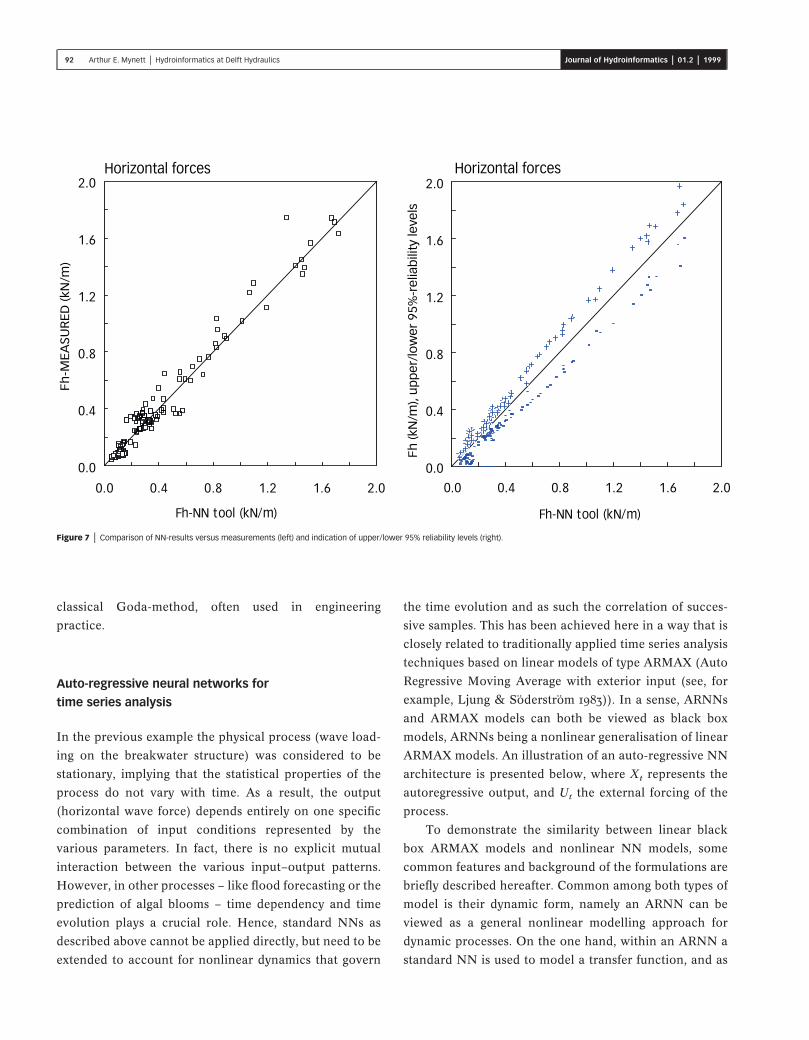
classical Goda-method, often used in engineering

practice.

Auto-regressive neural networks for

time series analysis

In the previous example the physical process (wave load-

ing on the breakwater structure) was considered to be

stationary, implying that the statistical properties of the

process do not vary with time. As a result, the output

(horizontal wave force) depends entirely on one specific

combination of input conditions represented by the

various parameters. In fact, there is no explicit mutual

interaction between the various input–output patterns.

However, in other processes – like flood forecasting or the

prediction of algal blooms – time dependency and time

evolution plays a crucial role. Hence, standard NNs as

described above cannot be applied directly, but need to be

extended to account for nonlinear dynamics that govern

the time evolution and as such the correlation of succes-

sive samples. This has been achieved here in a way that is

closely related to traditionally applied time series analysis

techniques based on linear models of type ARMAX (Auto

Regressive Moving Average with exterior input (see, for

example, Ljung & Soderstrom 1983)). In a sense, ARNNs

and ARMAX models can both be viewed as black box

models, ARNNs being a nonlinear generalisation of linear

ARMAX models. An illustration of an auto-regressive NN

architecture is presented below, where Xt represents the

autoregressive output, and Ut the external forcing of the

process.

To demonstrate the similarity between linear black

box ARMAX models and nonlinear NN models, some

common features and background of the formulations are

briefly described hereafter. Common among both types of

model is their dynamic form, namely an ARNN can be

viewed as a general nonlinear modelling approach for

dynamic processes. On the one hand, within an ARNN a

standard NN is used to model a transfer function, and as

��

��

��

��

��

��

��

��

�� !"#$%!&�'()*+,

��

��

��

��

��

��

��

��

��))��'()*+,

��'()*+,-��*��.��/01�� 2 � ��3��

��))��'()*+,

Figure 7 | Comparison of NN-results versus measurements (left) and indication of upper/lower 95% reliability levels (right).


such an ARNN is largely a data-driven modelling tech-

nique. On the other hand, however, conceptual (physical)

knowledge is explicitly contained in the state space form

of the ARNN, and hence can be seen as a step towards

introducing physically based modelling within NN

simulations.

Traditionally, linear black box models of type ARMAX

are frequently used in time series analysis. In discrete time

stepping procedures these models have a form where the

model’s response at time t depends linearly on the external

forcings at time t as well as at preceding time steps (t − 1,

t − 2, t − 3, . . .). The forcing may consist of deterministic

components as well as random components. Apart from

this linear regressive part with respect to the forcings also

a linear auto-regressive part is often included by feedback

of a linearly weighted sum of the outputs computed in one

or more preceding time steps. Randomness in the model’s

definition can be included to account for uncertainties in

the forcings and/or model uncertainties in more general

sense (system noise). Mathematically all this can be

expressed as

Xt = ∑k=1K akXt−k +∑l=0

L blUt−l +∑m=0M gmZt−m, (3.1)

where Xt represents the output process, Ut the determin-

istic forcing (input process), and Zt a random forcing

which is assumed to be white (i.e. Zt1 and Zt2 are statisti-

cally independent for t1 ≠ t2) and stationary. The par-

ameters ak, bl, gm are assumed to be constants. Clearly this

type of dynamic model is in complete parametrised form,

the weights in the regressive formulation being the

unknown parameters. For a proper initialisation of the

model, these parameters must be identified on the basis of

observed input–output combinations. See, for example,

Priestley (1992) and Gourbesville & Lecluse (1994) for

applications within hydrology.

In hydraulics, hydrology, ecology, etc. most concep-

tual dynamic models describing the time evolution of the

(spatially dependent) state variables have the form of one

or more coupled partial differential equations. They are

often written in a form with the first-order time derivatives

at the left-hand side and all the other terms at the right-

hand side. The terms at the right-hand side involve e.g.

convection and/or advection, friction, dispersion, reac-

tion, as well as terms that represent the contribution of

sinks and/or sources, or other model forcings such as

boundary conditions. Owing to nonlinearities and/or non-

constant or non-uniform coefficients these equations can-

not be solved analytically but must be discretized with

respect to time and the spatial coordinates. This leads to a

discrete time model in state space form:

Xt = F(Xt−1,Ut|a)+ Vt . (3.2)

Vector Xt represents the system’s state at discrete time t

and at one or more spatial positions (or even in distributed

form, e.g. the water levels and discharges at every grid-

point of a one-dimensional flow model of a branched river

system). Vector Ut represents the non-autonomous part

i.e. the system’s inputs or forcings (e.g. wind, lateral dis-

charges or boundary conditions). The (nonlinear) func-

tion F(·) represents a transfer function that governs the

dynamics of the system’s time evolution. In fact, it incor-

porates all the system knowledge that forms the basis of

the underlying conceptual model (and involves physical

principles such as conservation laws for mass, momentum,

energy, heat, etc.). The vector a represents unknown par-

ameters in the conceptual model that must be determined

by calibration. Vt is a random system noise, similar to the

ARMAX approach, that is included to account for uncer-

tainties in the forcings and/or model uncertainties in

general. In stochastic numerical models the inclusion of

system noise, together with uncertainties in observations

of the state variables, forms the basis for sequential

data-assimilation techniques (see, for example, Long

1989).

Clearly the dynamic models implied by Eqs(3.1) and

(3.2) have the same generic form in the sense that the

new state is determined from the preceding state(s) and

'�, ��4�'�, ��

' ,��4�

��' ,��4�

�' ,

�

��4�

�4�

�

�4��4� �

Figure 8 | Example of an Auto-Regressive NN of MLP architecture.


quantities that govern the system’s forcing. However, the

following differences should be mentioned:

1. The linear ARMAX-model is in fully parametrised

form, and the model as a whole must be identified

on the basis of a large set of observations. Hence

ARMAX is a black box model and a data-oriented

modelling technique. On the other hand, the

numerical state space model of Eq.(3.2) is usually

nonlinear and almost completely based on system

knowledge. It will contain only a (relatively) few

unknown parameters that originate from

uncertainties in one or more model coefficients

and/or (sub)processes. These parameters must also

be determined by means of calibration but because

of the knowledge-based form of modelling, a sparse

rather than a densely distributed measurement set

will often be sufficient.

2. In addition to (1) it can be also be mentioned that

ARMAX (as well as NN) models will be most

suitable for modelling the time evolution of a limited

number of state variables (e.g. time-dependent water

levels at one or a few spatial positions). They will

not be appropriate for the modelling of spatially

distributed processes (e.g. water levels and/or

currents on a large and dense two-dimensional

computational grid as described in the previous

section on computational modelling of flooding

systems), because this would require very large data

sets to provide all relevant spatial and temporal

correlations. In practice such distributed data sets

are not easy to obtain although remote sensing

techniques may provide important opportunities for

the near future.

3. The auto-regressive terms on the right-hand side of

the ARMAX-model of Eq.(3.1) may involve state

variables and forcings of more than one preceding

time steps. In the conceptual model of Eq.(3.2) this

‘horizon’ is at most one time step which is the result

of only first-order temporal derivatives in the

underlying partial differential equations defining the

conceptual model. It must be noted, however, that

conceptual models involving second- or higher-order

temporal derivatives (e.g. wave equations) can easily

be rewritten into a form with two or more coupled

equations of first order (in combination with an

appropriate extension of the state variables).

Sometimes this is also done within the ARMAX

approach to achieve that the model is

auto-regressive of order 1, and in this way enable

recursive (filtering) techniques for the identification

of its parameters (Ljung & Soderstrom 1983). Apart

from this, we must recall that ARMAX techniques

are often applied to model a system’s state at one or

a few spatial positions. Therefore the model cannot,

or only marginally, deal with, or ‘learn’ from spatial

correlations and to compensate this absence, all

information must be obtained from temporal

correlations suggesting (auto)regressive parts of

higher order.

In essence, the state space form is a common feature of the

dynamic models underlying both Eq.(3.1) and Eq.(3.2). At

the same time, however, these models are in some sense

opposite ‘extremes’ with respect to the origin of the trans-

fer function F(·): it is a fully parametrised and linear

function for the ARMAX models of Eq.(3.1), and a non-

linear function (almost) fully based on system knowledge,

in Eq.(3.2). Hence, recalling the property that NNs are

universal function approximators (Cybenko 1989), a pow-

erful generic form of a dynamic system can be obtained by

modelling the transfer function with a nonlinear NN. For

the general case of a K-dimensional multivariate time

series Xt as output, with the kth component auto-

regressive of order Mk (Mk ≥ 0), and an L-dimensional

external forcing Ut with the lth component regressive of

order Nl, and for the moment dealing with deterministic

models only, this leads to the following nonlinear

auto-regressive model:

Xt(1)

Xt(2)

·Xt

(k)

·Xt

(K)

=NN

Xt−1(1) , Xt−2

(1) , ··· , Xt−M1(1) ,

Xt−1(2) , Xt−2

(2) , ··· , Xt−M2(2) ,

· · ··· · ,Xt−1

(K) , Xt−2(K) , ··· , Xt−MK

(K) ,

U1(1) , Ut−1

(1) , ··· , Ut−N1(1) ,

Ut(2) , Ut−1

(2) , ··· , Ut−N2(2) ,

· · ··· · ,Ut

(L) , Ut−1(L) , ··· , Ut−NL

(L)

. (3.3)( ) ( )


The NN is a neural network (here assumed of type MLP)

with ∑Kk = 1Mk + ∑L

l = 0Nl neurons in the input layer and K

neurons in the output layer. The example shown in Figure 8

is an illustration of such a model where K = 2, M1 = 2,

M2 = 0, L = 1, and N1 = 2.

The dynamic model of Eq.(3.3) will be referred to as

an Auto-Regressive NN (ARNN). It is in state space form

and in this way a main property of conceptual numerical

models is explicitly incorporated in the description of

the time evolution of the involved processes. As a result

the system of Eq.(3.3) much more represents a model

in the strict sense, than the NNs used in standard form

where no time evolution or any other prior system

knowledge is taken into account.

The training of an ARNN will be a difficult problem

because the ensemble of input–output combinations is

mutually dependent, i.e. inputs determine the outputs and

vice versa, and the standard approach based on the error-

back-propagation-rule cannot be used anymore, and must

be generalised. It turns out that for this generalisation

the adjoint formalism known from data assimilation in

large-scale deterministic numerical models is most

appropriate.

Application to water balance in Lake IJsselmeer

An illustrative example of an ARNN application concerns

the modelling and prediction of the water balance of Lake

IJsselmeer in The Netherlands. In a more detailed form

this application is described by Gautam (1998). The most

important factors that affect the management of the water

balance are the inflow by the discharge of the river IJssel,

and the inner (lake side) and outer (sea side, i.e. the Dutch

Wadden Sea) water levels at the sluices of Den Oever and

Kornwerderzand. A plan view of the area is shown in

Figure 9. The difference of the inner and outer (tidal)

water levels determine when (e.g. at low tide) and how

long water can be drained from the lake into the Wadden

Sea, or vice versa. However, it must be taken into account

that the water levels can be significantly affected by

wind.

On this basis an ARNN was prepared with five forc-

ings as exterior inputs: the discharge of the river Ijssel; the

North–South and East–West components of the wind;

and the tidal water levels at the sluices of Kornwerderzand

and Den Oever. The (auto-regressive) output consists of

the water level of the IJsselmeer. The time step in the

model is �t = 1 day, adopted from the sampling rate for

which observations of the discharges of the river IJssel and

the lake’s water levels were available. For synchronisation

also the wind speeds and the outer tidal water levels were

represented by daily samples. Here this was done by taking

the daily maximum for the wind speed and the daily

minimum of the tidal water levels.

For the IJsselmeer area different target water levels are

maintained during summer and winter. Within the present

study only winter regimes were considered, which are

particularly interesting owing to their pronounced

dynamic behaviour. In this way the data ensemble consists

of daily samples within the periods 1 October until 31

March, for all 15 winter seasons from 1978–79 until

1992–93. From this ensemble nine seasons were chosen

for training and the other six seasons for verification. This

was done in such a way that the training and test ensemble

were statistically representative for the whole data set. On

the basis of repeated training sessions, systematically vary-

ing the orders in the model’s regressive part with respect

to the five forcings, and also varying the order in the

Figure 9 | Plan view Lake IJsselmeer.


auto-regressive part, followed by a comparison of the

model’s performance on the training set and the verifi-

cation set, the ‘optimal’ ARNN architecture was

determined. This turned out to be auto-regressive of order

1, second-order regressive with respect to the discharges

of the river IJssel, and 0th order (i.e. non-regressive) with

respect to the other forcings.

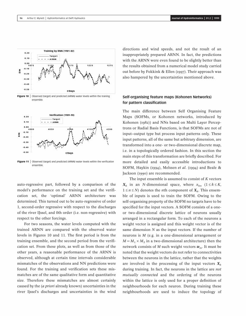
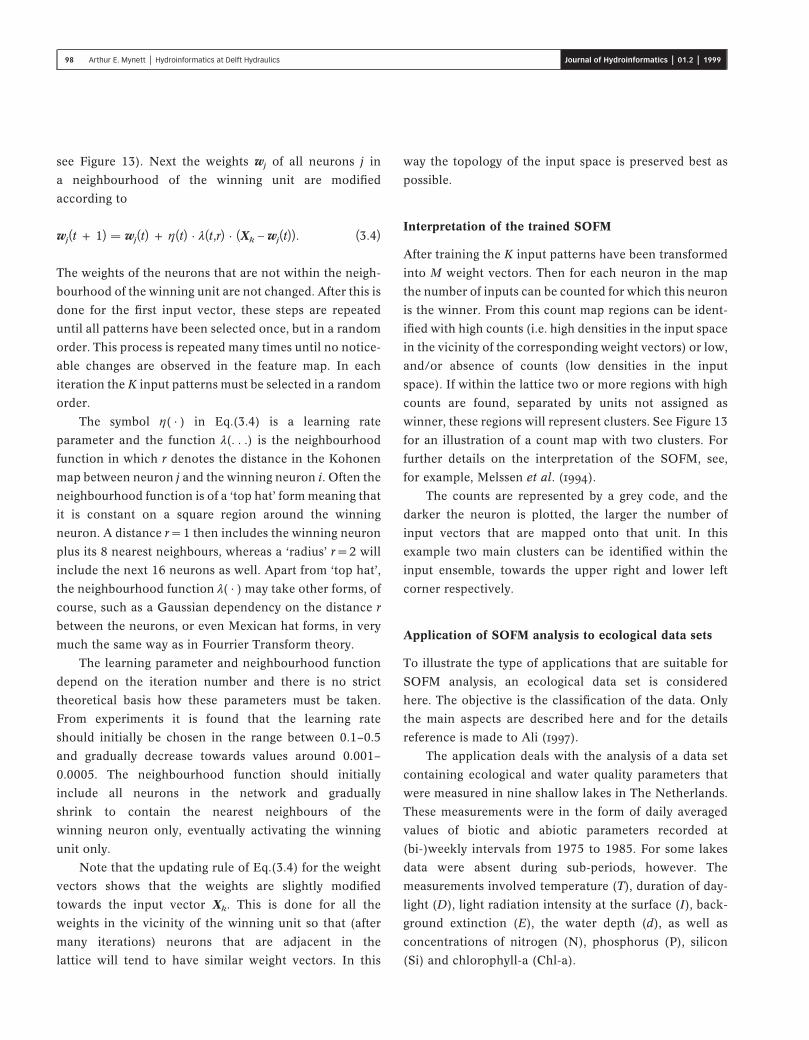
For two seasons, the water levels computed with the

trained ARNN are compared with the observed water

levels in Figures 10 and 11. The first period is from the

training ensemble, and the second period from the verifi-

cation set. From these plots, as well as from those of the

other years, a reasonable performance of the ARNN is

observed, although at certain time intervals considerable

mismatches of the observations and NN predictions were

found. For the training and verification sets these mis-

matches are of the same qualitative form and quantitative

size. Therefore these mismatches are almost certainly

caused by the (a priori already known) uncertainties in the

river Ijssel’s discharges and uncertainties in the wind

directions and wind speeds, and not the result of an

inappropriately prepared ARNN. In fact, the predictions

with the ARNN were even found to be slightly better than

the results obtained from a numerical model study carried

out before by Fokkink & Ellen (1997). Their approach was

also hampered by the uncertainties mentioned above.

Self-organising feature maps (Kohonen Networks)

for pattern classification

The main difference between Self Organising Feature

Maps (SOFMs, or Kohonen networks, introduced by

Kohonen (1982)) and NNs based on Multi Layer Percep-

trons or Radial Basis Functions, is that SOFMs are not of

input–output type but process input patterns only. These

input patterns, all of the same but arbitrary dimension, are

transformed into a one- or two-dimensional discrete map,

i.e. in a topologically ordered fashion. In this section the

main steps of this transformation are briefly described. For

more detailed and easily accessible introductions to

SOFM, Haykin (1994), Melssen et al. (1994) and Beale &

Jackson (1990) are recommended.

The input ensemble is assumed to consist of K vectors

Xk in an N-dimensional space, where xkn (1 ≤ k ≤ K,

1 ≤ n ≤ N) denotes the nth component of Xk. This ensem-

ble of inputs is used to train the SOFM. Owing to the

self-organising property of the SOFM no targets have to be

specified for the input vectors. A SOFM consists of a one-

or two-dimensional discrete lattice of neurons usually

arranged in a rectangular form. To each of the neurons a

weight vector is assigned and this weight vector is of the

same dimension N as the input vectors. If the number of

neurons is M (e.g. in a one-dimensional arrangement or

M =M1 ×M2 in a two-dimensional architecture) then the

network consists of M such weight vectors wm. It must be

noted that the weight vectors do not refer to connectivities

between the neurons in the lattice, rather that the weights

are involved in the processing of the input vectors Xk

during training. In fact, the neurons in the lattice are not

mutually connected and the ordering of the neurons

within the lattice is only used for a proper definition of

neighbourhoods for each neuron. During training these

neighbourhoods are used to induce the topology of

� � ��

��

��

��

��

� ��

� ��

� ��

� � � � � � � � � � � � � � � � �

��

� ��

� ��

��

��

Figure 10 | Observed (target) and predicted (ARNN) water levels within the training

ensemble.

� � � � � � � � � � � � � � � � � � � �

� ��

� ��

��

��

��

��

��

� ��

� ��

� ��

��

!��"�# ��$��

��

Figure 11 | Observed (target) and predicted (ARNN) water levels within the verification

ensemble.


the input ensemble into the set of weight vectors. An

illustration of a two-dimensional SOFM-architecture

(Kohonen Network) is given in Figure 12.

Training of the SOFM

Each neuron m in the network is fed by the input vector Xk

and is equipped with a single weight vector wm which is of

the same dimension as the input vectors. The arrows

represent the evaluation of the similarity between the

input vector and the weight vectors. The larger the

similarity, the more bold an arrow is plotted. Neuron i is

then the ‘winning’ unit. The dashed box denotes a neigh-

bourhood where during training the weights wj of the

enclosed units j are slightly adapted towards the input

vector Xk.

Before training of the SOFM can be started, a function

D(. . .) must be specified that Dmk = D(wm,Xk) measures

the similarity of a weight vector wm and an input vector

Xk. With this similarity measure the degree of agreement

(’similarity’) between two vectors is defined, varying from

‘equivalent’ to ‘totally different’. The similarity measure

will have a large effect on the classification process

because similar input vectors will after training refer to

the same, or neighbouring neurons in the feature map,

whereas very different inputs will activate neurons that are

far apart. With the similarity measure, however, the user

can bring in system knowledge and/or strategies to control

the classification process.

For the similarity measure several alternatives are

possible. Most common are distance measures, such as the

Euclidean distance, or non-Euclidean distance definitions

like the Minkowski distance. Also, distances may be taken

that involve scaling of one or more of the coordinates (or

even involve the inverse covariance matrix of the training

set) to obtain that in all directions the range of variation is

the same. Sometimes, also, similarity measures are used

based on the dot or inner product of the vectors, and apart

from possible normalisations of the input vectors, two

vectors are then similar if they are in the same direction.

Training of the SOFM, as for all types of NNs, implies

that the weights in the network are identified on the basis

of the input data set. In the SOFM the weight vectors are

often randomly initialised at the beginning of the training

process, but sometimes in some way use is made of (an

approximation of) the distribution of the input vectors, if

possible.

Then the following iteration is performed which will

be repeated many times (therefore the iteration is labelled

with a discrete time index t). An iteration starts with a

random selection of an input pattern Xk and for all the

neurons m (1 <m <M) in the lattice the similarity

measure Dmk is evaluated. Then the neuron i is selected

for which the similarity is maximal (the so called ‘winner’,

�� 5 ��

�

� �� 5

��

� �(

�� 3��

+

Figure 12 | Example of a two-dimensional 8×8 Kohonen Network.

Figure 13 | Example of a count map of a trained SOFM.


see Figure 13). Next the weights wj of all neurons j in

a neighbourhood of the winning unit are modified

according to

wj(t + 1) = wj(t)+ h(t) · l(t,r) · (Xk − wj(t)). (3.4)

The weights of the neurons that are not within the neigh-

bourhood of the winning unit are not changed. After this is

done for the first input vector, these steps are repeated

until all patterns have been selected once, but in a random

order. This process is repeated many times until no notice-

able changes are observed in the feature map. In each

iteration the K input patterns must be selected in a random

order.

The symbol h( · ) in Eq.(3.4) is a learning rate

parameter and the function l(. . .) is the neighbourhood

function in which r denotes the distance in the Kohonen

map between neuron j and the winning neuron i. Often the

neighbourhood function is of a ‘top hat’ form meaning that

it is constant on a square region around the winning

neuron. A distance r = 1 then includes the winning neuron

plus its 8 nearest neighbours, whereas a ‘radius’ r = 2 will

include the next 16 neurons as well. Apart from ‘top hat’,

the neighbourhood function l( · ) may take other forms, ofcourse, such as a Gaussian dependency on the distance r

between the neurons, or even Mexican hat forms, in very

much the same way as in Fourrier Transform theory.

The learning parameter and neighbourhood function

depend on the iteration number and there is no strict

theoretical basis how these parameters must be taken.

From experiments it is found that the learning rate

should initially be chosen in the range between 0.1–0.5

and gradually decrease towards values around 0.001–

0.0005. The neighbourhood function should initially

include all neurons in the network and gradually

shrink to contain the nearest neighbours of the

winning neuron only, eventually activating the winning

unit only.

Note that the updating rule of Eq.(3.4) for the weight

vectors shows that the weights are slightly modified

towards the input vector Xk. This is done for all the

weights in the vicinity of the winning unit so that (after

many iterations) neurons that are adjacent in the

lattice will tend to have similar weight vectors. In this

way the topology of the input space is preserved best as

possible.

Interpretation of the trained SOFM

After training the K input patterns have been transformed

into M weight vectors. Then for each neuron in the map

the number of inputs can be counted for which this neuron

is the winner. From this count map regions can be ident-

ified with high counts (i.e. high densities in the input space

in the vicinity of the corresponding weight vectors) or low,

and/or absence of counts (low densities in the input

space). If within the lattice two or more regions with high

counts are found, separated by units not assigned as

winner, these regions will represent clusters. See Figure 13

for an illustration of a count map with two clusters. For

further details on the interpretation of the SOFM, see,

for example, Melssen et al. (1994).

The counts are represented by a grey code, and the

darker the neuron is plotted, the larger the number of

input vectors that are mapped onto that unit. In this

example two main clusters can be identified within the

input ensemble, towards the upper right and lower left

corner respectively.

Application of SOFM analysis to ecological data sets

To illustrate the type of applications that are suitable for

SOFM analysis, an ecological data set is considered

here. The objective is the classification of the data. Only

the main aspects are described here and for the details

reference is made to Ali (1997).

The application deals with the analysis of a data set

containing ecological and water quality parameters that

were measured in nine shallow lakes in The Netherlands.

These measurements were in the form of daily averaged

values of biotic and abiotic parameters recorded at

(bi-)weekly intervals from 1975 to 1985. For some lakes

data were absent during sub-periods, however. The

measurements involved temperature (T), duration of day-

light (D), light radiation intensity at the surface (I), back-

ground extinction (E), the water depth (d), as well as

concentrations of nitrogen (N), phosphorus (P), silicon

(Si) and chlorophyll-a (Chl-a).


From the radiation intensity, depth and background

extinction the accumulated intensity parameter Ih =

I/(d × E) was determined. The chlorophyll concentration

is a measure of the algal mass present in the system and is

actually ‘determined’ by the other parameters. In the past,

either conceptual models or MLP type NNs were applied

to predict the chlorophyll level from the accumulated

intensity parameter Ih, and the remaining five forcings T,

N, P, Si, and D. Within the (preliminary) MLP-type appli-

cations, not so much attention was paid at first to a proper

validation analysis of this six-dimensional input ensemble.

To overcome this ‘omission’, the feasibility of SOFM for

such an analysis was investigated (Ali 1997). The main

results are summarised below.

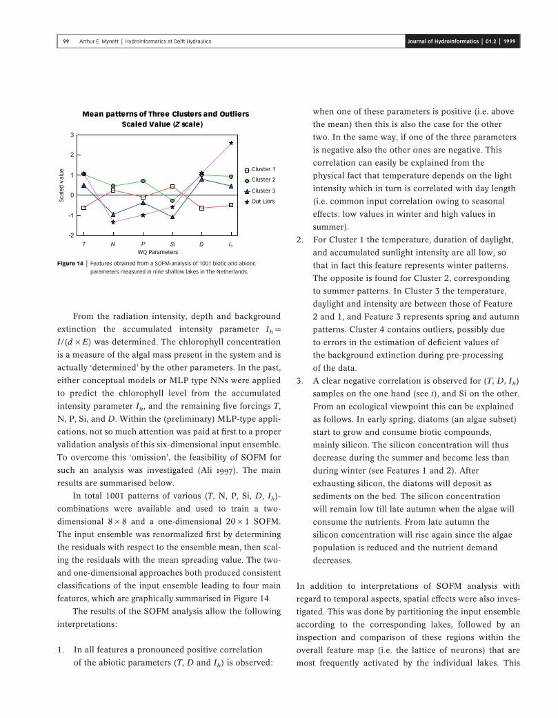
In total 1001 patterns of various (T, N, P, Si, D, Ih)-

combinations were available and used to train a two-

dimensional 8 × 8 and a one-dimensional 20 × 1 SOFM.

The input ensemble was renormalized first by determining

the residuals with respect to the ensemble mean, then scal-

ing the residuals with the mean spreading value. The two-

and one-dimensional approaches both produced consistent

classifications of the input ensemble leading to four main

features, which are graphically summarised in Figure 14.

The results of the SOFM analysis allow the following

interpretations:

1. In all features a pronounced positive correlation

of the abiotic parameters (T, D and Ih) is observed:

when one of these parameters is positive (i.e. above

the mean) then this is also the case for the other

two. In the same way, if one of the three parameters

is negative also the other ones are negative. This

correlation can easily be explained from the

physical fact that temperature depends on the light

intensity which in turn is correlated with day length

(i.e. common input correlation owing to seasonal

effects: low values in winter and high values in

summer).

2. For Cluster 1 the temperature, duration of daylight,

and accumulated sunlight intensity are all low, so

that in fact this feature represents winter patterns.

The opposite is found for Cluster 2, corresponding

to summer patterns. In Cluster 3 the temperature,

daylight and intensity are between those of Feature

2 and 1, and Feature 3 represents spring and autumn

patterns. Cluster 4 contains outliers, possibly due

to errors in the estimation of deficient values of

the background extinction during pre-processing

of the data.

3. A clear negative correlation is observed for (T, D, Ih)

samples on the one hand (see i), and Si on the other.

From an ecological viewpoint this can be explained

as follows. In early spring, diatoms (an algae subset)

start to grow and consume biotic compounds,

mainly silicon. The silicon concentration will thus

decrease during the summer and become less than

during winter (see Features 1 and 2). After

exhausting silicon, the diatoms will deposit as

sediments on the bed. The silicon concentration

will remain low till late autumn when the algae will

consume the nutrients. From late autumn the

silicon concentration will rise again since the algae

population is reduced and the nutrient demand

decreases.

In addition to interpretations of SOFM analysis with

regard to temporal aspects, spatial effects were also inves-

tigated. This was done by partitioning the input ensemble

according to the corresponding lakes, followed by an

inspection and comparison of these regions within the

overall feature map (i.e. the lattice of neurons) that are

most frequently activated by the individual lakes. This

��

��

�

�

�

�

67�8��+��

#��3��

� � � ��

9��

9��

9��5

��

%� ��& �� $"��'��()* �� +�,*�)�� -# )�+�! )*�� # )��

Figure 14 | Features obtained from a SOFM-analysis of 1001 biotic and abiotic

parameters measured in nine shallow lakes in The Netherlands.


allowed a rough classification of the lakes that could be

related to the measured chlorophyll concentrations in

these lakes. Moreover, for a few lakes, the inputs were

partitioned in time as well by no longer activating some

regions in the map over some period of time, thus simulat-

ing management strategies to reduce eutrophication in the

lakes. In this way a sudden trend as a result of the

management strategy could be clearly identified Although

the obtained trend was not really a surprise (since the

management strategy was known to have taken place), the

results nevertheless clearly confirmed its implications,

thus demonstrating the SOFM’s potential for general data

analysis and interpretation.

CONCLUSIONS AND REFLECTIONS ONFORTHCOMING DEVELOPMENTS

In this paper various applications of computer-based mod-

elling are presented. For problems that are well described

by mathematical equations, numerical simulation tech-

niques can be used. Examples are given for dam break

problems and for inundation of polders. When no explicit

mathematical formulation can be given, but when

adequate data are available, computer-based techniques

can be employed yet again. Data-driven modelling tech-

niques like NNs, developed in artificial intelligence, are

particularly useful for data analysis and pattern recog-

nition when no a priori knowledge of the underlying

processes is available. Several applications are shown

here, including horizontal wave forces on breakwaters,

water level predictions in lakes, and feature analysis of

ecological data sets. All examples are taken from recent

work at Delft Hydraulics, although only a limited selection

could be presented here. More elaborate contributions as

well as other topics can be expected in forthcoming issues

of this Journal.

Advances in the field of computational modelling

clearly demonstrate the feasibility of using numerical

simulation techniques for solving realistic problems (like

the inundation of polders). When the physical aspects are

well described by mathematical equations and the numeri-

cal scheme has been validated against experimental inves-

tigations and field observations (the IAHR working group

on dam break problems is one such validation forum),

computer simulations can provide valuable insight. In

particular, when the computational results are embedded

in a geographical information system environment and

the time evolution of the computed results is displayed

dynamically, the inundation process can easily be inter-

preted. In the near future a combined one-dimensional

network/two-dimensional horizontal flow simulation sys-

tem embedded in a GIS environment will become avail-

able, which can be applied to rural and urban area

flooding problems simultaneously. When incorporated

within a decision support system, alternatives for evacu-

ation plans and risk assessment can be explored directly.

Government authorities and insurance companies have

already expressed great interest in such systems. Several

directly relevant practical applications are likely to be

expected in the very near future. Moreover, the distributed

use of such advanced modelling systems via the Internet

will make them more accessible to practitioners and at the

same time better to maintain and update by developers

(see, for example, Mynett et al. 1998).

Diversification of computer-based modelling tech-

nologies to application areas where no clear mathematical

formulation may (yet) be present but where adequate data

sets are available, has been illustrated by several realistic

examples from engineering practice. Various applications

of one particular class of so-called subsymbolic tech-

niques, namely Artificial Neural Networks (ANNs),

clearly demonstrate the power of such approaches

(Boogaard et al. 1998a,b). Although often presented as

‘black box modelling’, it should be stressed, however, that

adequate knowledge and experience is often also required

here, if reliable and practicable answers are to be

obtained. For example, input–output relations have to be

imposed, which implies at least some a priori knowledge

on cause–effect relations. This is not always trivial in

dynamic ecosystems, however. Also, choosing the proper

number of layers in an MLP-type network is very much

related to the amount of data available for training and

verification, if under- or overtraining is to be avoided.

However, dependencies may be present within the data

set. Hence, pre-processing and classification of data,

introduced here as an application of self-organising


feature maps (Kohonen Networks), can be a very valuable

first step in NN modelling. Combinations of various tech-

niques are being explored as well. In general, alternative

computational modelling techniques like ‘neuro-fuzzy

computing’ are developing rapidly and practical examples

of such approaches may be expected in the near future.

The same applies to optimization techniques for decision

support when evaluating complex dynamic systems:

whether based on a ‘constraint logic’ approach or on

‘evolutionary computing’, new developments are under

way to become relevant methodologies in engineering

practice.

ACKNOWLEDGEMENTS

The material presented here is largely a compilation of

ongoing work at Delft Hydraulics. All colleagues involved

are fully credited for their contributions. Special thanks

are due to Professor G. S. Stelling and Dr H. F. P. van den

Boogaard for their support. More extensive elaborations

on the material summarised here can be obtained from

their references.

REFERENCES

Abbott, M. B. 1991 Hydroinformatics – Information Technology andthe Aquatic Environment. Avebury Technical, Aldershot, UK.

Abbott, M. B. 1993 The electronic encapsulation of knowledge inhydraulics, hydrology and water resources. Adv. Wat. Resour.No. 16, 21–39.

Abbott, M. B. 1994 Hydroinformatics: A Copernican revolutionin hydraulics. J. Hydraulics Res. 32 (3) (Extra Issue), 3–13.

ACM Communications, March 1994, 37 (3).Alcrudo, F. & Garcia-Navarro, P. 1993 A high-resolution

Godunov-type scheme in finite volumes for the 2-d shallowwater equations. Int. J. Num. Meth. in Fluids 16.

Ali, Md A. 1997 Applications of Self Organising Feature Mapsfor the Analysis of Hydrological and Ecological Data Sets.M.Sc. Thesis, H.H.315, IHE, Delft, The Netherlands.

Babovic, V. 1996 Emergence, Evolution, Intelligence:Hydroinformatics. Ph.D. Thesis, Balkema, Rotterdam.

Babovic, V. & Larsen, L. C. 1996 (eds) Hydroinformatics ’98, 2 vols,ISBN 90 5410 983 1. Balkema, Rotterdam,

Beale, R. & Jackson, T. 1990 Neural Computing: An Introduction.Bristol: IOP Publishing.

Boogaard, H. F. P. van den, A. E. Mynett, A. E. & Ali, Md S. 1998aSelf organizing feature maps for the analysis of hydrologicaland ecological data sets. In Hydroinformatics ’98 (ed.Babovic, V. M. & Larsen, L. C.), pp. 733–740. Balkema,Rotterdam.

Boogaard. H. F. P. van den, Gautam, D. K. & Mynett, A. E. 1998bAuto-regressive neural networks for the modelling of timeseries. In Hydroinformatics ’98 (ed. Babovic, V. M. & Larsen,L. C.), pp 741–748. Balkema, Rotterdam.

Casulli, V. 1990 Semi-implicit fin. dif. met. for two-dimensionalshal.water eq. J. Comput. Phys. 86, pp 56.

Chaudry, M. H. 1993 Open-Channel Flow. Prentice Hall.Cybenko, G. 1989. Approximation by superpositions of a

sigmoidal function. Math. Control Signals Systems 2,303–314.

Falconer, R. A. & Chen, Y. 1991 An improved repres. of flooding anddrying and wind stress effects in a two-dimensional tidal num.Model. Proc. Inst. Civ. Engrs, part 2, pp. 659.

Fokkink, R. & van Ellen, W. 1997 SOBEK-BEKKEN computations forthe water management within the IJsselmeer area. [In Dutch.]WLzDELFT HYDRAULICS, report T2179.

Gautam, D. K. 1998 Regressive Neural Networks for themodelling of time series. MSc Thesis, IHE, Delft,The Netherlands.

Gent, M. R. A. van & Boogaard, H. F. P. van den 1998 NeuralNetwork and Numerical Modelling of Forces on VerticalStructures. MAST/PROVERBS-report. WLzDELFT HYDRAULICS, Delft,The Netherlands.

Gourbesville, P. & Lecluse, Y. 1994 STORAGE: A STochasticmultimOdel pRocedure for dischArGe forEcasting.In Hydroinformatics ’94 (ed. Verwey, Minns,Babovic & Maksimovic), pp. 147–154. Balkema,Rotterdam.

Hall, M. J. & Minns, A. W. 1993 Rainfall-runoff modelling as aproblem in artificial intelligence: experience with a neuralnetwork. In Proc. 4th Nat. Hydrol. Symp, 5.51–5.57, Cardiff.British Hydrological Society, London.

Haykin, S. 1994 Neural Networks. A Comprehensive Foundation.New York, Macmillan.

Hirsch, C. 1990 Numerical Computation of Internal and ExternalFlows. John Wiley.

Ippen, A.T. 1966 Estuary and Coastline Hydrodynamics.McGraw-Hill.

Kernkamp, H. W. J. & de Jonge, J. J. de 1997 Test reservoir models.Q2136/Z993, Delft Hydraulics.

Kohonen, T. 1982 Self organized formation of topologically correctfeature maps. Biological Cybernetics 43, 59–69.

Lambert, J. D. 1991 Numerical Methods for Ordinary DifferentialSystems. John Wiley.

Leendertse, J. J. 1967 Aspects of a comp. model for long periodwater-wave propagation. RAND Corp. MemorandumRM-5294-PR.

Ljung, L. & Soderstrom, T. 1983 Theory and Practice of RecursiveIdentification. New York, MIT Press.

Long, R. B. 1989 Notes on assimilating observations into numericalmodels. WLzDelft Hydraulics, Report Z274.


Mase, H., Sakamoto, M. & Sakai, T. 1995 Neural network forstability analysis of rubble-mound breakwaters. J. of Waterway,Port, Coastal and Ocean Engng, ASCE, November/December1995, 294–299.

Melssen, W.J., Smits, J. R. M., Buydens, L. M. C. & Kateman, G.1994 Using artificial neural networks for solving chemicalproblems. Part II. Kohonen self-organising feature mapsand Hopfield networks. Chemometrics and IntelligentLaboratory Systems 23, 267–291.

Minns, A.W. 1998 Artificial Neural Networks as Subsymbolic ProcessDescriptors. PhD. Thesis, Delft University of Technology.

Mueller, A. (Ed) 1996 Hydroinformatics ’96, ISBN 90 5410 852 5.Balkema, Rotterdam.

Mynett, A. E., Hummel, S. & Elshoff, I. J. P. & Cate, H. H. ten 1998Distributed computing systems in environmentalhydroinformatics: applications in engineering and in education.In Hydroinformatics ’98 (ed. Babovic, V. M. & Larsen, L. C.),pp. 949–955. Balkema, Rotterdam.

Priestley, M. B. 1992 Spectral Analysis and Time Series. London,Academic Press.

Recknagel, F., French, M., Harkonen, P. & Yanunaka, K. I. 1997Artificial neural network approach for modelling andprediction of algal blooms. Ecological Modelling 96,11–28.

Rouse, H. (Ed.) 1950 Engineering Hydraulics, p. 130. New York,John Wiley.

Scardi, M. 1996 Artificial neural networks as empirical models forestimating phytoplankton production. Marine Ecol. Progr.Ser. 139, 289–299.

Stelling, G. S., Wiersma, A. & Willemse, J. 1986 Practical aspects ofaccurate tidal computations. J. ASCE Hyd. Eng., No. 9, pp. 802.

Stelling, G. S., Kernkamp, H. W. J. & Laguzzi, M.M. 1998 DelftFlooding System: a powerful tool for inundation assessmentbased upon a positive flow simulation. In Hydroinformatics ’98(ed. Babovic, V. M. & Larsen, L. C.) pp. 449–456. Balkema,Rotterdam.

Toro, E. F. 1997 Riemann Solvers and Numerical Methods for FluidDynamics, Springer.

Verwey, A., Minns, A. W., Babovic, V. & Maksimovic, C. (eds) 1994Hydroinformatics ’94, ISBN 90 5410 512 7. Balkema, Rotterdam.


Hydroinformatics and its applications at Delft Hydraulics

Documents

Transcript of Hydroinformatics and its applications at Delft Hydraulics