Hybridization of Multi-Objective Evolutionary Algorithms and ArtificialNeural Networks for Optimizing the Performance of Electrical Drives

Alexandru-Ciprian Zavoianu a,c Gerd Bramerdorfer b,c Edwin Lughofer a Siegfried Silber b,c

Wolfgang Amrhein b,c Erich Peter Klement a,c

aDepartment of Knowledge-based Mathematical Systems/Fuzzy Logic Laboratory Linz-Hagenberg, Johannes Kepler University of Linz,Austria

bInstitute for Electrical Drives and Power Electronics, Johannes Kepler University of Linz, AustriacACCM, Austrian Center of Competence in Mechatronics, Linz, Austria

Abstract

Performance optimization of electrical drives implies a lot of degrees of freedom in the variation of design parameters, which in turnmakes the process overly complex and sometimes impossible to handle for classical analytical optimization approaches. This, andthe fact that multiple non-independent design parameter have to be optimized synchronously, makes a soft computing approachbased on multi-objective evolutionary algorithms (MOEAs) a feasible alternative. In this paper, we describe the application ofthe well known Non-dominated Sorting Genetic Algorithm II (NSGA-II) in order to obtain high-quality Pareto-optimal solutionsfor three optimization scenarios. The nature of these scenarios requires the usage of fitness evaluation functions that rely on verytime-intensive finite element (FE) simulations. The key and novel aspect of our optimization procedure is the on-the-fly automatedcreation of highly accurate and stable surrogate fitness functions based on artificial neural networks (ANNs). We employ thesesurrogate fitness functions in the middle and end parts of the NSGA-II run (→ hybridization) in order to significantly reducethe very high computational effort required by the optimization process. The results show that by using this hybrid optimizationprocedure, the computation time of a single optimization run can be reduced by 46% to 72% while achieving Pareto-optimalsolution sets with similar, or even slightly better, quality as those obtained when conducting NSGA-II runs that use FE simulationsover the whole run-time of the optimization process.

Key words: electrical drives, performance optimization, multi-objective evolutionary algorithms, feed-forward artificial neural networks,

surrogate fitness evaluation, hybridization

1. Introduction

1.1. Motivation

Today, electrical drives account for about 70% of the to-tal electrical energy consumption in industry and for about40% of used global electricity [1]. In [2] it is stated that,each year, in the European Union, the amount of wastedenergy that could be saved by increasing the efficiency ofelectrical drives is around 200TWh and for this reason, in2009, a European regulation was concluded forcing a grad-ual increase of the energy efficiency of electrical drives [3].However, manufacturers of electrical machines need to takemore than just the efficiency into account to hold theirown value in the global market. To be able to successfullycompete, the electrical drives should be fault-tolerant andshould offer easy to control operational characteristics and

compact dimensions. Apart from these, the most impor-tant quality factor is the price. During the development ofan electrical machine, a multi-objective optimization ap-proach [4,5] is required in order to address all of the aboveaspects and to find an appropriate tradeoff between the fi-nal efficiency and the cost of the drive.

1.2. State-of-the-Art in Electrical Drive Design

In the past, electrical machines were designed by ap-plying a parameter sweep and calculating a maximum ofseveral hundred designs [6]. Calculating a design actuallymeans predicting the operational behavior of the electri-cal drive for a concrete set of parameter settings. Becauseof the nonlinear behavior of the materials involved, sucha prediction needs to be based on time intensive finite el-ement simulations. This, combined with the need to have

Preprint submitted to Engineering Application of Artificial Intelligence 1 July 2013

an acceptable duration of the overall analysis, imposed asevere limitation in the number of designs to be calculated.As such, only major design parameters could be taken intoconsideration and only a rather coarse parameter step sizecould be applied.

During the last decade, the use of response surfacemethodology [7], genetic algorithms [8,9], particle swarmoptimization [10] and other techniques [11] for the designof electrical machines and the associated electronics hasbecome state-of-the-art. For a detailed comparisons ofthese modern approaches and additional reviews of thestate-of-the-art in electrical drive design, the reader iskindly directed to consult [12–14].

Although the above mentioned search methods haveproved to be far more suitable for the task of multi-objective optimization than basic parameter sweeps, theyare still plagued by the huge execution times incurredby the need to rely on FE simulations throughout theoptimization procedure. The usage of computer clusterswhere multiple FE simulations can be performed in par-allel can partially address this problem, but the followingdrawbacks still remain severe:– The FE evaluation of one particular design still takes

a long time and conventional methods need to evaluateeach individual design.

– There are high costs associated with the usage of com-puter clustering architectures and various software li-censes.

1.3. Our Approach

In our attempt to create an efficient optimization frame-work for electrical drive design, we are exploiting wellknown and widely applied genetic algorithms used formulti-objective optimization. These specialized algorithmsare generally able to efficiently handle several optimiza-tion objectives. For us, these objectives are electrical drivetarget parameters like efficiency, cogging torque, total ironlosses, etc. In our implementation, the goal is to minimizeall the objectives. If a target needs to be maximized in thedesign (e.g., efficiency), during the optimization, its neg-ative value is taken to be minimized. The FE simulationsrequired by each fitness function evaluation are distributedover a high throughput computer cluster system. Althoughit is able to evolve electrical drive designs of remarkablehigh quality, the major drawback of this initial, and some-what conventional, optimization approach (ConvOpt)is that it is quite slow as it exhibits overall optimizationrun-times that vary from ≈ 44 to ≈ 70 hours. As a par-ticular multi-objective genetic algorithm, we employ thewell-known and widely used NSGA-II[15].

One main method aimed at improving the computationaltime of a multi-objective evolutionary algorithm that hasa very time-intensive fitness function is to approximate theactual function through means of metamodels / surrogatemodels [16]. These surrogate models can provide a very

accurate estimation of the original fitness function at afraction of the computational effort required by the latter.Three very well documented overviews on surrogate basedanalysis and optimization can be found in [17], [18] and [19].

In our case, the idea is to substitute the time-intensivefitness functions based on FE simulations with very-fast-to-evaluate surrogates based on highly accurate regressionmodels. The surrogate models act as direct mappings be-tween the design parameters (inputs) and the electric drivetarget values which should be estimated (outputs). For us,in order to be effective in their role to reduce overall op-timization run-time, the surrogate models need to be con-structed on-the-fly, automatically, during the run of theevolutionary algorithm. This is because they are quite spe-cific for each optimization scenario and each target value(i.e., optimization goal or optimization constraint) that weconsider.

In other words, we would like that only individuals (i.e.,electrical drive designs) from the first N generations willbe evaluated with the time-intensive FE-based fitness func-tion. These initial, FE evaluated, electrical drive designswill form a training set for constructing the surrogate mod-els. For the remaining generations, the surrogate modelswill substitute the FE simulations as the basis of the fit-ness function. As our tests show, this yields a significantreduction in computation time.

The novelty of our research lies in the analysis of howto efficiently integrate automatically created on-the-fly-surrogate-models in order to reduce the overall optimiza-tion run-time without impacting the high quality of theelectrical drive designs produced by ConvOpt.

Artificial Neural Networks (ANNs) [20] are among thepopular methods used for constructing surrogate modelsbecause they possess the universal approximation capabil-ity [21] and they offer parameterization options that allowfor an adequate degree of control over the complexity ofthe resulting model. Another advantage of ANNs is the factthat they are known to perform well on non-linear and noisydata [22] and that they have already been successfully ap-plied in evolutionary computation for designing surrogatemodels on several instances [23,24]. For the purpose of thisresearch, the particular type of ANN we have chosen to useis the multilayered perceptron (MLP). MLP is a popularand widely used neural network paradigm that has beensuccessfully employed to create robust and compact pre-diction models in many practical applications [25,26]. How-ever, our choice for the MLP is first and foremost motivatedby the fact that, for our specific modeling requirements,MLP-bases surrogate models have proved to be both rela-tively fast and easy to create as well as extremely accurate.

There is a wide choice of methods available for construct-ing surrogate models. In this paper, we describe in detailshow we created surrogates based on MLPs, but our hy-bridization schema itself is general and suitable for a multi-tude of modeling methods. In Section 5.1 we present resultsobtained with other non-linear modeling methods that canbe used as alternatives for constructing the surrogate mod-

2

els. These modeling methods are, support vector regression(SVR) [27], RBF networks [28] and a regression orientatedadaptation of the instance based learning algorithm IBk[29]. In the aforementioned section, we also further moti-vate our current preference for MLP surrogate models.

Regardless of the modeling method used, the automaticsurrogate model construction phase involves testing differ-ent parameter settings (e.g. different number of neuronsand learning rates in the case of MLPs, different values of Cand γ in the case of SVR), yielding many models with dif-ferent complexities and prediction behaviors. Given a cer-tain target parameter we propose a new, automated modelselection criterion, aimed at selecting the best surrogateto be integrated in the optimization process. The selectedsurrogate model should deliver the best tradeoff betweensmoothness, accuracy and sensitivity, i.e., the lowest pos-sible complexity with an above-average predictive quality.

The rest of this paper is organized in the following way:Section 2 presents an overview of multi-objective optimiza-tion problems (MOOPs) in general with a special focuson the particular complexities associated with MOOPs en-countered in the design and prototyping of electrical drives.Section 3 contains a description of our hybrid optimizationprocedure (HybridOpt) focusing on the creation and in-tegration of the MLP surrogate models. Section 4 providesthe description of the experimental setup. Section 5 con-tains an evaluation of the performance of the hybrid op-timization process with regards to the overall run-time ofthe simulations and the quality of the obtained solutions.Section 6 concludes the paper with a summary of achievedand open issues.

2. Problem Statement

The design of an electrical machine usually comprises atleast the optimization of geometric dimensions for a pre-selected topology. Figure 1 gives the cross-section of anelectrical drive featuring a slotted stator with concentratedcoils and an interior rotor with buried permanent magnets.The geometric parameters of this assembly are depicted inthe figure (dsi, bst, bss. etc.). Depending on the actual prob-lem setting, usually, most of these parameters need to bevaried in order to achieve a cheap motor with good op-erational behavior. Furthermore, due to the fast movingglobal raw material market, companies tend to investigatethe quality of target parameters with regard to differentmaterials. Sometimes, the study of different topologies isalso required during the design stage. All these lead to arelatively high number of input parameters for the opti-mization procedure.

Furthermore, because the behavior of the materials usedto construct the electrical drive cannot be modeled linearly,the evaluation of a given design has to be done by usingcomputationally expensive FE simulations. These are solv-ing non-linear differential equations in order to obtain thevalues of the target parameters associated with the actual

(a) Stator

(b) Rotor

Fig. 1. Geometric dimensions of the stator and rotor for an interiorrotor topology with embedded magnets

design parameter vector. Specifically, we use the softwarepackage FEMAGTM[30] for the calculation of 2D problemson electro-magnetics.

As our main goal is the simultaneous minimization of allthe objectives (target values) involved, we are faced witha multi-objective optimization problem which can be for-mally defined by:

min (o1(X), o2(X), ..., ok(X)), (1)

where

o1(X), o2(X), ..., ok(X) (2)

are the objectives (i.e. target parameters) that we considerand

XT =[x1 x2 . . . xn

](3)

is the design parameter vector (e.g. motor typology identi-fier, geometric dimensions, material properties, etc).

3

Additionally, hard constraints like (4) can be specifiedin order to make sure that the drive exhibits a valid op-erational behavior (e.g. the torque ripple is upper bound).Such constraints are also used for invalidating designs witha very high price.

c(x) ≤ 0 ∈ Rm (4)

In order to characterize the solution of MOOPs it is help-ful to first explain the notion of Pareto dominance [31]:Definition 1 Given a set of objectives, a solution A is saidto Pareto dominate another solution B if A is not inferiorto B with regards to any objectives and there is at least oneobjective for which A is better than B.

The result of an optimization process for a MOOP isusually a set of Pareto-optimal solutions named the Paretofront [31] (a set where no solution is Pareto dominated byany other solution in the set). The ideal result of the multi-objective optimization is a Pareto front which is evenlyspread and situated as close as possible to the true Paretofront of the problem (i.e., the set of all non-dominated so-lutions in the search space).

3. Optimization Procedure

3.1. Conventional Optimization using Multi-ObjectiveEvolutionary Algorithms

As most evolutionary algorithms (EAs) work generation-wise for improving sets (populations) of solutions, variousextensions aimed at making EA populations store and ef-ficiently explore Pareto fronts have enabled these types ofalgorithms to efficiently find multiple Pareto-optimal solu-tions for MOOPs in one single run. Such algorithms arereferred to as multi-objective evolutionary algorithms orMOEAs in short.

In our case, each individual from the MOEA populationwill be represented as a fixed length real parameter vectorthat is actually an instance of the design parameter vec-tor described in (3). Computing the fitness of every suchindividual means computing the objective functions from(2) and, at first, this can only be achieved by running FEsimulations.

The Non-dominated Sorting Genetic Algorithm II(NSGA-II) [15] proposed by K. Deb in 2002 is, along-side with the Strength Pareto Evolutionary Algorithm 2(SPEA2) [32], one of the most successful and widely ap-plied MOEA algorithms in literature. A brief description ofNSGA-II is presented in Appendix A. On a close review, itis easy to observe that both mentioned MOEAs are basedon the same two major design principles:

(i) an elitist approach to evolution implemented using asecondary (archiving) population;

(ii) a two-tier selection for survival function that usesa primary Pareto non-dominance metric and a sec-ondary density estimation metric;

In light of the above, it is not surprising that the respec-tive performance of these two algorithms is also quite simi-lar [32,33] with minor advantages towards either of the twomethods depending on the particularities of the concreteMOOP problem to be solved [34,35]. Taking into accountthe similarity of the two MOEAs and the very long execu-tion time required by a single optimization run, we mentionthat all the tests reported on over the course of this re-search have been carried out using NSGA-II. Our choice forthis method is also motivated by a few initial comparativeruns in which the inherent ability of NSGA-II to amplifythe search around the extreme Pareto front points enabledit to find a higher number of very interesting solutions thanSPEA2 for two of our optimization scenarios.

3.2. Hybrid Optimization using a Fitness Function basedon Surrogate Models

3.2.1. Basic IdeaOur main approach to further improve the run time

of the our optimization process is centered on substitut-ing the original FE-based fitness function of the MOEAswith a fitness function based on surrogate models. Themain challenge lies in the fact that these surrogate mod-els, which must be highly accurate, are scenario depen-dent and as such, for any previously unknown optimiza-tion scenario, they need to be constructed on-the-fly (i.e.,during the run of the MOEA). A sketch of the surrogate-based enhanced optimization process (HybridOpt) outlin-ing the several new stages it contains in order to incorporatesurrogate-based fitness evaluation is presented in Figure 2.

In the FE-based MOEA execution stage the first N gen-erations of each MOEA run are computed using FE simu-lations and all the individuals evaluated at this stage willform the training set used to construct the surrogate mod-els. Each sample in this training set contains the initialelectrical motor design parameter values (3) and the cor-responding objective function values (2) computed usingFEMAGTM. Please refer to Section 5.2 for a descriptionof the methodology we used in order to determine a goodvalue of N .

In the surrogate model construction stage, we use system-atic parameter variation and a selection process that takesinto consideration both accuracy and architectural simplic-ity to find and train the most robust surrogate design foreach of the considered target variables.

The next step is to switch the MOEA to a surrogate-based fitness function for the remaining generations that wewish to compute (surrogate-based MOEA execution stage).The surrogate-based fitness function is extremely fast whencompared to its FE-based counterpart, and it enables theprediction of target values based on input variables withinmilliseconds. Apart from improving the total run time ofthe MOEA simulation, we can also take advantage of thismassive improvement in speed in two other ways:

(i) by increasing the total number of generations the

4

Fig. 2. Diagram of the conventional optimization process - ConvOpt and of the surrogate-enhanced optimization process - HybridOpt when

wishing to compute a total of M generations

MOEA will compute during the simulation;(ii) by increasing the sizes of the populations with which

the MOEA operates;Both options are extremely important as they generallyenable MOEAs to evolve Pareto fronts that are larger insize and exhibit a better spread.

In the surrogate-based Pareto front computation stagea preliminary surrogate-based Pareto front is extractedonly from the combined set of individuals evaluated usingthe surrogate models. This secondary Pareto front is con-structed independently, i.e., without taking into considera-tion the quality of the FE-evaluated individuals in the firstN generations. Initial tests have shown that this approachmakes the surrogate-based front less prone to instabilitiesinduced by inherent prediction errors and by the relativedifferences between the qualities of the surrogate models.

We mention that, in the current stage of development,at the end of the MOEA run (the FE-based reevaluationstage), it is desired that all the Pareto-optimal solutionsfound using the surrogate models are re-evaluated using FEcalculations. There are two main reasons for which we dothis. The first one is a consequence of the fact that in ouroptimization framework, the check for geometry errors istightly coupled with the FE evaluation stage and as suchsome of the Pareto optimal solutions found using the sur-rogate models might actually be geometrically invalid. Thesecond reason for the re-evaluation is to assure that all thesimulation solutions presented as Pareto optimal have thesame approximation error (i.e., the internal estimation er-ror of the FEMAGTMsoftware).

In the final Pareto front computation stage, the finalPareto front of the simulation is extracted from the com-bined set of all the individuals evaluated using FE simula-

tions, i.e., individuals from the initial N generations andFE-reevaluated surrogate-based individuals.

It is important to note that our enhanced optimizationprocess basically redefines the role of the FE simula-tions. These very accurate but extremely time intensiveoperations are now used at the beginning of the MOEAdriven optimization process, when, generally, the quality-improvement over computation time ratio is the highest.FE simulations are also used in the final stage of the op-timization process for analyzing only the most promisingindividuals found using the surrogate models. In the mid-dle and in the last part of the optimization run, whenquality improvements would come at a much higher com-putational cost, a surrogate-based fitness function is usedto steer the evolutionary algorithm.

In the results section, we will show that, using the sur-rogate enhancement, Pareto fronts with similar quality tothe ones produced by ConvOpt can be obtained while sig-nificantly reducing the overall simulation time.

3.2.2. The Structure and Training of ANN SurrogateModels

Generally, the MLP architecture (Figure 3) consists ofone layer of input units (nodes), one layer of output unitsand one or more intermediate (hidden) layers. MLPs im-plement the feed-forward information flow which directsdata from the units in the input layer through the unitsin the hidden layer to the unit(s) in the output layer. Anyconnection between two units ui and uj has an associatedweight wij that represents the strength of that respectiveconnection. A concrete MLP prediction model is definedby its specific architecture and by the values of the weightsbetween its units.

5

Given the unit ui, the set Pred(ui) contains all the unitsuj that connect to node ui, i.e. all the units uj for whichwji exists. Similarly, the set Succ(ui) contains all the unitsuk to which node ui connects to, i.e. for which wik exists.

Each unit ui in the network computes an output valuef(ui) based on a given set of inputs. Depending on howthis output is computed, one may distinguish between twotypes of units in a MLP:

(i) Input units - all the units in the input layer. The roleof these units is to simply propagate into the networkthe appropriate input values from the data sample wewish to evaluate. In our case, f(ui) = xi where xi isthe ith variable of the design parameter vector from(3).

(ii) Sigmoid units - all the units in the hidden and outputlayers. These units first compute a weighted sum ofconnections flowing into them (5) and then producean output using a non-linear logistic (sigmoid shaped)activation function (6):

s(ui) =∑

uj∈Pred(ui)

wjif(uj) (5)

f(ui) = P (ui) =1

1 + e−s(ui)(6)

In our modeling tasks, we use MLPs that are fully con-nected, i.e. for every sigmoid unit ui, Predui

exclusivelycontains all the units in the previous layer of the network.In the input layer, we use as many units as design variablesin the data sample. Also, as we construct a different sur-rogate model for each target variable in the data sample,the output layer contains just one unit and, at the end ofthe feed-forward propagation, the output of this unit is thepredicted regression value of the elicited target (e.g. P (o1)for the MLP presented in Figure 3).

The weights of the MLP are initialized with small randomvalues and then are subsequently adjusted during a trainingprocess. In this training process we use a training set Tand every instance (data sample) −→s ∈ T contains both thevalues of the varied design parameters (i.e., XT ) as well asthe FE-computed value of the elicited target variable (e.g.,syFE

is the FE estimated value of o2(X) from (2) wheno2(X) is the target for which we wish to construct a MLPsurrogate model):

−→s = (x1, x2, . . . , xn, yFE) (7)

The quality of the predictions made by the MLP can beevaluated by passing every instance from the training setthrough the network and then computing a cumulative er-ror metric (i.e., the batch learning approach). When con-sidering the MLP architecture presented in Figure 3 andthe squared-error loss function, the cumulative error met-ric over training set T is:

E(−→w ) =1

2

∑−→s ∈T

(syFE− P (o1(sxi ,

−→w )))2, i = 1,m (8)

Fig. 3. Multilayer perceptron model with one hidden layer and one

output unit

The goal of the training process is to adjust the weightssuch as to minimize this error metric. The standard ap-proach in the field of ANNs for solving this task is the back-propagation algorithm [36] which is in essence a gradient-based iterative method that shows how to gradually adjustthe weights in order to reduce the training error of the MLP.

First, at each iteration t, the error metric Et(−→w ) is com-puted using (8). Afterwards, each weight wt

ij in the MLPwill be updated according to the following formulas:

∆wtij = ηδ(uj)P (ui)

wtij = wt

ij + ∆wtij if t = 1

wtij = wt

ij + ∆wtij + α∆wt−1

ij if t > 1

(9)

where η ∈ (0, 1] is a constant called the learning rate. Byα ∈ [0, 1), we mark the control parameter of the empiri-cal enhancement known as momentum, which can help thegradient method to converge faster and to avoid some lo-cal minima. The function δ(uj) shows the cumulated im-pact that the weighted inputs coming into node uj have onEt(−→w ) and is computed as:

δ(uj) = P (uj)(1− P (uj))(y − P (uj)) (10)

if uj is the output unit and as:

δ(uj) = P (uj)(1− P (uj))∑

uk∈Succ(uj)

δukwjk (11)

if uj is a hidden unit. The standard backpropagationmethod proposes several stopping criteria: the number ofiterations exceeds a certain limit, Et(−→w ) becomes smallerthan a predefined ε, the overall computation time exceeds acertain pre-defined threshold. We have chosen to adopt anearly stopping mechanism that terminates the executionwhenever the prediction error computed over a validation

6

subset V does not improve over 200 consecutive iterations.This validation subset is constructed at the beginning ofthe training process by randomly sampling 20% of theinstances from the training set T . This stopping criterionmay have a benefit in helping to prevent the overfitting ofMLP surrogate models.

3.2.3. The Evaluation and Automatic Model Selection ofANN Surrogate Models

Usually, in MLP-based data modeling tasks the most im-portant design decision concerns the network architecture:how many hidden layers to use and how many units to placein each hidden layer. In order to construct a highly accu-rate model, based on the previous architecture choice, oneshould also experiment with several values for the learningrate and momentum constants. In practice, this problemis most often solved by experimentation usually combinedwith some sort of expert knowledge.

It has been shown that MLPs with two hidden layerscan approximate any arbitrary function with arbitrary ac-curacy [37] and that any bounded continuous function canbe approximated by a MLP with a single hidden layer anda finite number of hidden sigmoid units [38]. The optimiza-tion scenarios used in this research (see Section 4.1) do notrequire the use of two hidden layers. Like with many otherinterpolation methods, the quality of the MLP approxima-tion is dependent on the number of training samples thatare available and on how well they cover the input space. Inour application, we have the flexibility to select the numberof samples used for training the surrogate model accordingto the complexity of the learning problem (i.e., number ofdesign parameters and their associated range values) andthis aspect is detailed in Section 5.2.

In order to automatically determine the number of hid-den units, the learning rate (η) and the momentum (α)needed to construct the most robust MLP surrogate model,we conduct a best parameter grid search, iterating over dif-ferent parameter value combinations (see Section 4.2 forexact settings).

Our model selection strategy is aimed at finding the mostaccurate and robust surrogate model where, by robust, weunderstand a model that displays a rather low complex-ity and a stable predictive behavior. Our tests have shownthat these two qualities are very important when strivingto construct surrogate models that enable the MOEAs tosuccessfully explore the entire search space.

The surrogate model selection process (Figure 4) is di-vided in two stages. In the first stage, all the surrogatesare ranked according to a metric that takes into accountthe accuracy of their predictions. Next, an accuracy thresh-old is computed as the mean of the accuracies of the bestperforming 2% of all surrogate models. The choice of thefinal surrogate model is made using a complexity metricthat favors the least complex model that has a predictionaccuracy higher than the accuracy threshold. The generalidea is similar to that of a model selection strategy used for

Fig. 4. Diagram of the surrogate model selection process where the

predictive accuracy of the model is computed according to (12)

regression trees [39] with the noticeable difference that wecompute the accuracy threshold using a broader model ba-sis in order to increase stability (i.e., avoid the cases wherethe accuracy threshold is solely set according to a highlycomplex, and possibly overfit, model that is only marginallymore accurate than several much simpler ones).

The metric used to evaluate the prediction accuracy ofa surrogate model qm, is based on the coefficient of deter-mination (R2). In order to evaluate the accuracy of a MLPsurrogate model we use a 10-fold cross-validation data par-titioning strategy [40] and we compute the value of R2 overeach of the ten folds. The final accuracy assigned to the sur-rogate model is the mean value of R2 minus the standarddeviation of R2 over the folds:

qm = µ(R2)− σ(R2) (12)

Using the standard deviation ofR2 over the cross-validationfolds as a penalty in (12) has the role of favoring modelsthat exhibit a more stable predictive behavior. The rea-son for this is that a significant value of σ(R2) indicatesthat the surrogate model is biased toward specific regionsof the search space. The existence of locally-biased surro-gate models is quite probable because our training data israther unbalanced as it is the byproduct of a highly elitistevolutionary process that disregards unfit individuals.

The second metric used in the surrogate model selectionprocess favours choosing less complex models. One MLPsurrogate model is considered to be more complex thananother if the former has more units in the hidden layer(ties are broken in favor of the model that required morecomputation time to train).

It is worth mentioning that this automatic surrogatemodel selection strategy can easily be adapted when opt-ing for another surrogate modeling method. In this case,one only needs to choose a different indicator (or set of in-dicators) for measuring complexity (e.g. the C parameterand/or the number of required support vectors in the caseof a SVR).

7

Algorithm 1 Description of the hybrid optimization process

1: procedure HybridOpt(Scenario, PopSizeini, PopSizeext, N,M)2: P ← RandomlyInitializePopulation(Scenario, PopSizeini)3: E ≡ FE-Evaluator(Scenario)4: 〈P, V alidFE〉 ← NSGA-II-Search(N,PopSizeini, P, E)5: Configurations← InitializeMlpGridSearchConfigurations6: for all target ∈ Scenario do7: Map← ∅8: for all c ∈ Configurations do9: Map←Map∪ ConstructSurrogateModel(c, target, V alidFE)

10: end for11: BestSurrogateModels(target)← SelectBestSurrogateModel(Map)12: end for13: E ≡ SurrogateEvaluator(Scenario,BestSurrogateModels)14: 〈P, V alidMLP 〉 ← NSGA-II-Search(M −N,PopSizeext, P, E)15: OptimalSetMLP ← ExtractParetoFront(V alidMLP )16: E ≡ FE-Evaluator(Scenario)17: OptimalSetMLP ← EvaluateFitness(OptimalSetMLP , E)18: return ExtractParetoFront(V alidFE ∩OptimalSetMLP )19: end procedure

20: function NSGA-II-Search(NrGen, PopSize, InitialPopulation, F itnessEvaluator)21: t← 122: V alidIndividuals← ∅23: P (t)← InitialPopulation24: P (t)← EvaluateFitness(P (t), F itnessEvaluator)25: while t ≤ NrGen do26: O(t)← CreateOffspring(P (t), PopSize)27: O(t)← EvaluateFitness(O(t), F itnessEvaluator)28: V alidIndividuals← V alidIndividuals ∪O(t)29: P (t+ 1)← ComputeNextPopulation(P (t), O(t), PopSize)30: t← t+ 131: end while32: return 〈P (t), V alidIndividuals〉33: end function

3.2.4. Algorithmic Description of HybridOptOur hybrid optimization procedure is presented in Algo-

rithm 1. Apart from method calls and the normal assign-ment operator (←), we also use the operator ≡ in order tomark the dynamic binding of a given object to a specificmethod with the implied meaning that all future referencesto the object are redirected to the corresponding targetedmethod.

The main procedure, named HybridOpt, has five inputparameters:– Scenario - the description of the scenario to be optimized

with information regarding design parameters and tar-gets

– PopSizeini - the size of the NSGA-II population for theFE-based part of the run

– PopSizeext - the size of the NSGA-II population for thesurrogate-based part of the run

– N - the number of generations to be computed in theFE-based part of the run

– M - the total number of generations to be computed

during the optimization (i.e., M −N generations will becomputed in the surrogate-based part)The NSGA-II implementation contained in the NSGA-

II-Search function differs from standard implementationsas it returns two results, the Pareto optimal set obtainedafter constructing the last generation and a set containingall the valid individuals generated during the search. Thisfunction has four input parameters:– NrGen - the number of generations to be computed– PopSize - the size of the population– InitialPopulation - a set containing the starting popu-

lation of the evolutionary search– FitnessEvaluator - an object that is bound to a specific

fitness evaluation functionThe method EvaluateFitness is of particular impor-

tance. It receives as input a set of unevaluated individualsand an object that is bound to a specific fitness evaluationfunction. EvaluateFitness returns a filtered set contain-ing only the valid individuals. Each individual in the re-turned set also stores information regarding its fitness over

8

the multiple objectives — note that the fitness is directlyassociated with the values of the target parameters, whichare either predicted by the surrogate model or calculatedusing differential equations in the FE simulation. If the con-crete fitness function used is FE-Evaluator, individualsare checked for validity with regards to both geometrical(meshing) errors and constraint satisfaction (4). Geomet-rical errors may arise because of specific combinations ofdesign parameter values. When using the SurrogateE-valuator, only constraint satisfaction validity checks canbe performed.

The other methods that we use in HybridOpt are:– RandomlyInitializePopulation - this method ran-

domly initializes a set of individuals of a given size ac-cording to the requirements of the optimization scenarioto be solved

– InitializeMlpGridSearchConfigurations - thismethod constructs all the MLP training configurationsthat are to be tested in a best parameter grid search (seeSection 4.2 for details)

– ConstructSurrogateModel - this method builds asingle MLP surrogate model for a given target based ona preset MLP training configuration and a training setof previously FE-evaluated individuals as described inSection 3.2.2

– SelectBestSurrogateModel - this method selectsthe most robust surrogate from a given set of modelsaccording to the surrogate model selection process de-scribed in Section 3.2.3

– ExtractParetoFront - this method extracts thePareto-optimal front from a given set of possible solu-tions after the description in Section 3.1.In the NSGA-II-Search method, the functions Cre-

ateOffspring and ComputeNextPopulation are re-sponsible for implementing the evolutionary mechanism de-scribed in Appendix A.

4. Experimental Setup

4.1. The Optimization Scenarios

We consider three multi-objective optimization scenarioscoming from the field of designing and prototyping electri-cal drives:

The first scenario (Scenario OptS1 ) is on a motor forwhich the rotor and stator topologies are shown in Figure1. The design parameter vector has a size of six and is givenby

XT =[hm αm er dsi bst bss

],

where all parameters are illustrated in Fig. 1 except forαm, which denotes the ratio between the actual magnetsize and the maximum possible magnet size as a result ofall other geometric parameters of the rotor. The targets forthe MLP surrogate model construction stage are the four,unconstrained, Pareto objectives:

– T1 = −η - where η denotes the efficiency of the motor. Inorder to minimize the losses of the motor, the efficiencyshould be maximized and therefore −η is selected forminimization.

– T2 = TcogPP - the peak-to-peak-value of the motortorque for no current excitation. This parameter de-notes the behavior of the motor at no-load operationand should be as small as possible in order to minimizevibrations and noise due to torque fluctuations.

– T3 = TotalCosts- the material costs associated with aparticular motor. Obviously, minimizing this objective isa very important task in most optimization scenarios.

– T4 = TrippPP - the equivalent of Tcog,PP at load opera-tion. The values of this objective should also be as smallas possible.The second problem (Scenario OptS2 ) is on an electrical

machine featuring an exterior rotor. The design parame-ter vector contains seven geometric dimensions. The aim ofthis optimization problem was to minimize the total lossesof the system at load operation and to minimize the to-tal mass of the assembly while simultaneously maintainingother desired operational characteristics (e.q., efficiency,cogging torque, costs, etc). In the case of this scenario, thefirst target (T1) is a hard-constrained Pareto optimizationgoal, the second (T2) is an unconstrained Pareto optimiza-tion goal, whilst the third (T3) is a secondary hard con-straint imposed on the evolved motor designs.

The third problem (Scenario OptS3 ) also concerns a mo-tor with an exterior rotor. The design parameter vector hasa size of ten. This scenario proposes four, hard-constrained,Pareto optimization goals. All of them are considered tar-gets in the surrogate model construction phase:– T1 = ls - the total axial length of the assembly– T2 = TotalMass - the total mass of the assembly– T3 = PCu- the ohmic losses in the stator coils– T4 = Pfe - the total losses due to material hysteresis and

eddy currents in the ferromagnetic parts of the motor

4.2. The Testing Framework

In order to compare the performance of the two optimiza-tion processes we are using optimization runs that compute100 generations with a population size of 50. This rathersmall choice of the population size is motivated by restric-tions regarding time and the available cluster computationpower for running the required simulations.

In order to illustrate some immediate benefits of usingthe enhanced approach (see Section 3.2.1), we also per-formed tests where, during the run of the MOEA, after theconstruction of the mappings, we doubled the populationsize and the number of generations to be evolved.

Our optimization framework uses the NSGA-II imple-mentation provided by the jMetal package [41]. For all testsreported in Section 5, we used NSGA-II with a crossoverprobability of 0.9, a crossover distribution index of 20, amutation probability of 1/|XT | and a mutation distribu-

9

tion index of 20. The high values of the distribution in-dexes for the crossover and mutation operators (that arerecommended by literature [15] and set as default in jMetal)force NSGA-II to generate near parent values for almost allspawned offspring. While this parameter choice seems todetermine an overall search strategy that favors exploita-tion over exploration, the highly elitist nature of NSGA-IIcoupled with the high mutation probability, help to bal-ance the exploitation versus exploration ratio over the en-tire run. Using ConvOpt, we have performed a tuning phaseto check whether smaller values (i.e., 15, 10, 5 and 2) forthe crossover and mutation distribution indexes would yieldbetter results when using a population size of 50 and alimited number of evolved generations. The results showedthat using these smaller index values does not produce anyimprovement.

In the case of HybridOpt, we perform the mapping train-ing stage after N = 25 generations (please see Section 5.2for a detailed explanation of this parameter choice). As weuse a population size of 50, the maximum possible size ofthe training sets is 1250 samples. The size of the actualtraining sets we obtained was smaller because some of theevolved design configurations were geometrically unfeasibleor invalid with regards to given optimization constraints.When considering all the performed tests, the average sizesand standard deviations of the obtained training sets is pre-sented in Table 1.

Table 1

The average size and standard deviations of the obtained trainingsets.

Scenario Training set size µ Training set size σ

OptS1 1219.50 22.40

OptS2 813 123.59

OptS3 743.25 74.33

The MLP implementation we used for our tests is largelybased on the one provided by the WEKA open source ma-chine learning platform [42]. In the case of the best param-eter grid searches that we performed in order to create theMLP surrogate models:– the number of hidden units was varied between 2 and

double the number of design variables;– η was varied between 0.05 and 0.40 with a step of 0.05– α was varied between 0.0 and 0.7 with a step of 0.1

The search is quite fine grained as it involves buildingbetween 704 (scenario OptS1 ) and 1216 (scenario OptS3 )MLP surrogate models for each elicited target. This ap-proach is possible because we make use of the early stoppingmechanism in the MLP training process (see Section 3.2.2)which in turn ensures an average surrogate model trainingtime of 356.70 seconds. We achieve a considerable speedupin the surrogate model creation stage by distributing all theMLP training tasks over the same high throughput clustercomputing environment that is used to run in parallel theFE simulations. As a result, the surrogate model creation

stage took, on average, 146.33 minutes, over all performedtests.

4.3. Considered Performance Metrics

In order to compare the performance and behavior of theconventional and hybrid optimization processes we use fourperformance metrics:

(i) the hypervolume metric H [43] measures the overallcoverage of the obtained Pareto set;

(ii) the generalized spread metric S [44] measures the rel-ative spatial distribution of the non-dominated solu-tions;

(iii) the FE utility metric U offers some insight on theefficient usage of the FE evaluations throughout theoptimization;

(iv) the run-time metric T records the total runtime inminutes required by one optimization;

The hypervolume and generalized spread metrics arecommonly used in MOEA literature when comparing be-tween different non-dominated solution sets. The H metrichas the added advantage that it is the only MOEA metricfor which we have theoretical proof [45] of a monotonicbehavior. This means that the maximization of the hyper-volume constitutes the necessary and sufficient conditionfor the set of solutions to be “maximally diverse Paretooptimal solutions of a discrete, multi-objective, optimiza-tion problem”. By design, the upper bound of H is 1.00.For any optimization problem, the true Pareto front yieldsthe highest H value. As we are not dealing with artificialproblems, for our considered scenarios, the best possiblevalue of H for each problem is unknown.

In the case of the S metric, a value closer to 0.0 indi-cates that the solutions are evenly distributed in the searchspace. Although this metric is not monotonic in showingtrue Pareto front convergence, in our case, it is extremelyuseful as it is a good indicator of the diversity of Pareto-optimal electrical drive designs that our optimization runsare able to find.

The FE utility metric is constructed for the purpose ofillustrating how efficiently the optimization process is us-ing the very time intensive FE simulations over an entirerun. The U metric is computed as the ratio between thetotal number of non-dominated solutions found during theoptimization (i.e. the size of the final Pareto front) and thetotal number of performed FE simulations.

5. Results

5.1. Overview of MLP Surrogate Model Performance

In order to offer a quick insight into the characteristics ofthe elicited target variables, Table 3 contains the compar-ative results of trying to model the targets using linear re-gression, MLPs and three other non-linear modeling meth-ods. We considered sets containing all the samples obtained

10

(a) Scenario OptS1

(b) Scenario OptS2

(c) Scenario OptS3

Fig. 5. Evolution of the coefficient of determination computed overthe remaining 100−n generations for the best MLP surrogate models

trained using the first n ≤ 50 generations

using FE simulations over 100 NSGA-II generations with apopulation size of 50 and split them into training and testdata sets. The training data sets contain the individualsfrom the first 33 generations while the test data sets aremade up from the individuals from the last 67 generations(i.e., a ”1/3 - training , 2/3 - test” data set partitioningscheme). After removing the geometrically unfeasible andinvalid designs, we ended up with training sets of size 1595(OptS1 ), 1197 (OptS2 ), and 1103 (OptS3 ).

For the non-linear modeling methods, we report the testresult achieved by the best surrogate model which was se-

lected based on 10-fold cross-validation performance afterdoing a best parameter grid search on the training data.In the case of the MLP, the grid search was set up as de-scribed in Section 4.2. In the case of SVR, we trained 675surrogate models for each target as we varied: the gen-eral complexity parameter C between [2−4, 2−3, ..., 210],the RBF kernel parameter γ between [2−5, 2−4, ..., 23]and the ε parameter of the ε-intensive loss function be-tween [0.001, 0.005, 0.01, 0.025, 0.05]. For RBF networks,we trained 918 surrogate models for each target by varyingthe number of clusters between [2, 3, 4, 5, 10, 20, ..., 500]and the allowed minimum standard deviation for the clus-ters between [0.25, 0.5, 1.00, 2.00, ...15.0]. When using IBkmodeling, we created 900 surrogate models for each targetas we varied the number of nearest neighbors from 1 to 300and we used three different distance weighting options: noweighting, weight by 1/distance and weight by 1-distance.

Firstly, one can observe that while most targets dis-play a strong linear dependency towards their respectivedesign variables, the surrogate models obtained using lin-ear regression for some targets (e.g., OptS1-T1, OptS1-T2,OptS1-T4, OptS3-T4 ) are by no means accurate. For thepurpose of this research, we decided on a linear regressionR2 threshold value of 0.9 in order to classify a target aslinear or non-linear.

When considering only the six non-linear targets, MLPsand SVR are the best performers (MLP slightly better thanSVR) while RBF networks produce results that are signif-icantly worse. We conducted all the best parameter gridsearches by distributing the surrogate model training tasksover the computer cluster. We measured the time requiredby the grid searches conducted for non-linear targets and,for each modeling method, averaged it over the total num-ber of surrogate models to be trained. We present these re-sults in Table 2 and, together with some model complexityinformation, they indicate that, when comparing with theMLP:– RBF networks and SVR require ≈ 15% and ≈ 55% more

(wall) time in order to finish the grid search.– when taking into acount the sizes of the training sets,

RBF networks and SVR seem to produce surrogate mod-els that are quite complex (i.e., number of clusters re-quired by the RBF network and number of support vec-tors used by SVR)The difference in required training time, the low struc-

tural complexity, and the higher accuracy motivate ourchoice of using MLP surrogate models.

5.2. The Accuracy and Stability of MLP Surrogate ModelPredictions

In the current version of HybridOpt, it is very importantto choose a good value for the parameter N that indicatesfor how many generations we wish to run the initial FE-based execution stage. A value of the parameter that is toolow will result in creating inconclusive training sets which

11

Table 2Information regarding the average training time of the surrogate models and the structural complexity (i.e., number of hidden units in the

case of MLP, number of support vectors in the case of SVR and number of clusters in the case of RBF networks) of the best surrogate model

on the non-linear targets

TargetAverage training time [minutes] Complexity indicator of the best surrogate

MLP SVR RBF Nets MLP SVR RBF Nets

OptS1-T1

0.734 1.241 0.865

11 892 500

OptS1-T2 12 754 500

OptS1-T4 11 1046 500

OptS2-T1 0.678 0.931 0.620 9 323 300

OptS3-T30.601 0.945 0.837

12 858 400

OptS3-T4 10 868 400

All non-linear 0.671 1.039 0.774 10.83 790.16 433.33

Table 3Linear and non-linear regression modeling results on the elicited targets

Scenario Target ClassificationR2 on test instances

Linear MLP SVR RBF Nets IBk

OptS1

T1 non-linear 0.7353 0.9864 0.9330 0.9029 0.8744

T2 non-linear 0.6048 0.9530 0.9540 0.8992 0.9040

T3 linear 0.9777 0.9992 0.9997 0.9999 0.9660

T4 non-linear 0.6390 0.9674 0.9640 0.9099 0.9044

OptS2

T1 non-linear 0.8548 0.9923 0.9960 0.9859 0.9749

T2 linear 0.9916 0.9997 0.9997 0.9998 0.9904

T3 linear 0.9990 0.9999 0.9998 0.9999 0.9254

OptS3

T1 linear 0.9970 0.9999 0.9997 0.9999 0.9689

T2 linear 0.9514 0.9998 0.9995 0.9999 0.8822

T3 non-linear 0.8526 0.9799 0.9839 0.9804 0.8791

T4 non-linear 0.8355 0.9564 0.9552 0.9521 0.8794

Average All linear 0.9830 0.9997 0.9997 0.9997 0.9466

Average All non-linear 0.7540 0.9720 0.9640 0.9384 0.9026

Average All all 0.8580 0.9847 0.9802 0.9664 0.9226

in turn will lead to surrogate models that are not globallyaccurate or stable. By choosing a value for N that is a lothigher than the optimal one, we are more or less ”wasting”FE simulations by creating oversized training sets. In orderto choose a good value of N we take into account the influ-ence that this parameter has on the accuracy and stabilityof the resulting MLP surrogate models.

In order to estimate the influence that N has on the ac-curacy of the surrogate models, for each optimization sce-nario we consider fully FE-based runs of 100 generationsand the combined pools of samples that each such simula-tion produces. We construct 50 different test cases and, foreach target of each scenario, we divide the available sam-ples into a training and a test set. For test number i, thetraining set contains the individuals from the first i gener-ations and the validation set contains the individuals fromthe last 100− i generations. For each test, we use the bestparameter grid search and the automated model selection

strategy in order to obtain the best MLP surrogate modelon the training data. Next, we evaluate the quality of thissurrogate model by computing the coefficient of determi-nation over the corresponding test set. The resulting val-ues are plotted in Figure 5. It can be easily observed thatall targets display a stable logarithmic saturation behaviorthat suggests that a choice of N in the 20 to 30 generationsrange should be able to produce highly accurate surrogatemodels for all considered targets.

The concrete decision for the value of N is based on thestability over time of the obtained surrogate models. We es-timate the stability over time by computing the individualR2 of every generation in the test data sets. For example,Figure 6 contains the plots of the generational coefficientsof determination for the most difficult to model targets ofscenarios OptS1 and OptS3 (i.e., OptS1-T2 and OptS3-T4 ). We are only interested in the best surrogate modelsconstructed using the samples from the first 20 to 30 gen-

12

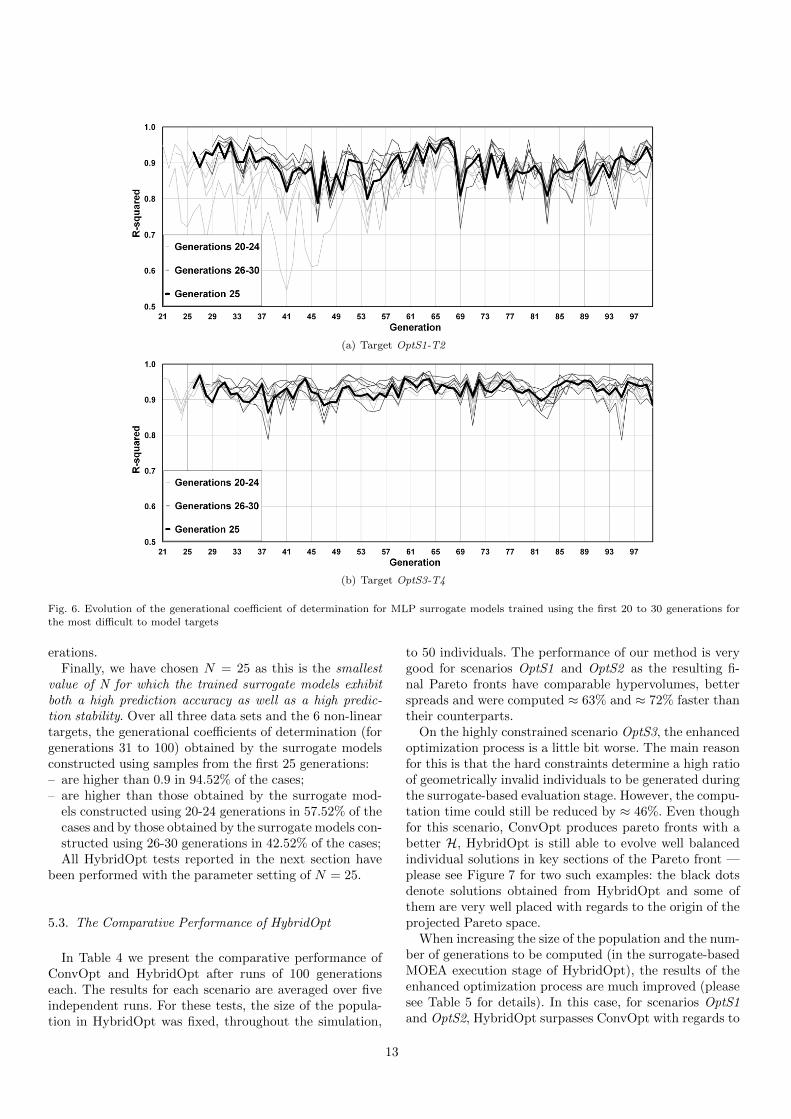
(a) Target OptS1-T2

(b) Target OptS3-T4

Fig. 6. Evolution of the generational coefficient of determination for MLP surrogate models trained using the first 20 to 30 generations for

the most difficult to model targets

erations.Finally, we have chosen N = 25 as this is the smallest

value of N for which the trained surrogate models exhibitboth a high prediction accuracy as well as a high predic-tion stability. Over all three data sets and the 6 non-lineartargets, the generational coefficients of determination (forgenerations 31 to 100) obtained by the surrogate modelsconstructed using samples from the first 25 generations:– are higher than 0.9 in 94.52% of the cases;– are higher than those obtained by the surrogate mod-

els constructed using 20-24 generations in 57.52% of thecases and by those obtained by the surrogate models con-structed using 26-30 generations in 42.52% of the cases;All HybridOpt tests reported in the next section have

been performed with the parameter setting of N = 25.

5.3. The Comparative Performance of HybridOpt

In Table 4 we present the comparative performance ofConvOpt and HybridOpt after runs of 100 generationseach. The results for each scenario are averaged over fiveindependent runs. For these tests, the size of the popula-tion in HybridOpt was fixed, throughout the simulation,

to 50 individuals. The performance of our method is verygood for scenarios OptS1 and OptS2 as the resulting fi-nal Pareto fronts have comparable hypervolumes, betterspreads and were computed ≈ 63% and ≈ 72% faster thantheir counterparts.

On the highly constrained scenario OptS3, the enhancedoptimization process is a little bit worse. The main reasonfor this is that the hard constraints determine a high ratioof geometrically invalid individuals to be generated duringthe surrogate-based evaluation stage. However, the compu-tation time could still be reduced by ≈ 46%. Even thoughfor this scenario, ConvOpt produces pareto fronts with abetter H, HybridOpt is still able to evolve well balancedindividual solutions in key sections of the Pareto front —please see Figure 7 for two such examples: the black dotsdenote solutions obtained from HybridOpt and some ofthem are very well placed with regards to the origin of theprojected Pareto space.

When increasing the size of the population and the num-ber of generations to be computed (in the surrogate-basedMOEA execution stage of HybridOpt), the results of theenhanced optimization process are much improved (pleasesee Table 5 for details). In this case, for scenarios OptS1and OptS2, HybridOpt surpasses ConvOpt with regards to

13

all the considered performance metrics.In the case of scenario OptS3, the increase of the post-

surrogate-creation population and of the number of gener-ations to be evaluated enable HybridOpt to surpass Con-vOpt with regards to the spread of the generated Paretofronts. The hyper-volume values, although much better, arestill 4-8% worse than those of ConvOpt.

As the increase in population size and number of gener-ations is directly translated into a higher number of indi-viduals that need to be re-evaluated using FE-simulations,the improvement in computation time is reduced to valuesranging from ≈ 14% to ≈ 69%. The reduction is partic-ularly visible in the case of the hard-constrained scenarioOptS3, where the amount of geometrically invalid individ-uals generated in the surrogate-based execution stage alsogrows substantially.

(a) Pareto front nr. 1

(b) Pareto front nr. 2

Fig. 7. 2D projections of the full Pareto fronts generated using Con-vOpt and HybridOpt for the highly constrained scenario OptS3. The

regions of the fronts with well balanced Pareto optimal designs are

magnified.

6. Conclusion

In this paper, we investigated multi-objective optimiza-tion algorithms based on evolutionary strategies, exploitingconcepts from the famous and widely used NSGA-II algo-rithm, for the purpose of optimizing the design of electricaldrives in terms of efficiency, costs, motor torque behavior,total mass of the assembly, ohmic losses in the stator coils

and others. Despite the parallelization of the whole opti-mization process over a computer cluster, as both the de-sign and the target parameter space can be quite large, verylong optimization runs are required in order to solve thecomplex scenarios that we deal with. This is because thefitness function used by NSGA-II search requires very time-intensive FE simulations in order to estimate the quality ofa given motor design.

In order to alleviate the problem, we experimented witha system that automatically creates, on-the-fly, non-linearsurrogate models that act as direct mappings between thedesign and the target parameters of the electrical drive.These surrogate models form the basis of a very fast to sur-rogate fitness function that replaces the original FE-basedfitness for the latter part of the optimization process. Em-pirical observations over averaged results indicate that thisleads to a reduction of the total run-time of the optimiza-tion process by 46-72%. For setting up the non-linear sur-rogate models, we applied multi-layer perceptron (MLP)neural networks, as they turned out to be more efficient interms of accuracy versus training and evaluation time thanother soft computing techniques.

The tests that we have performed show that, on aver-age, the Pareto fronts obtained using the hybrid, surrogate-enhanced approach, are similar (or even slightly better)than those obtained by using the conventional NSGA-IIoptimization process, which uses only the FE-based fitnessevaluation function. This may come as a surprise becausewhen we shift the optimization process to the surrogate-based fitness function, the optimization algorithm will infact try to converge to a new, surrogate-induced, artificialoptimum. The high quality of the MLP surrogate modelswe obtain directly translates into the fact that the artificialoptimum lies in the vicinity of the true (FE-induced) opti-mum. The close proximity of the two optima is the likelyreason for which the surrogate models are always able toefficiently steer the optimization process towards exploringhigh-quality Pareto fronts (as the results in Section 5.3 in-dicate).

Future work will basically focus on two issues:(i) Reducing the importance and the sensitivity of the

N parameter in HybridOpt by shifting our optimiza-tion algorithm towards an active learning approach.The idea is that initial surrogate models may beset up from fewer generations, than the currentlysuggested 25 and, from time to time, during thesurrogate-based MOEA execution stage, certain in-dividuals (or generations) are to be evaluated byFE-simulations. This dual evaluation (surrogate andFE-based) will provide information for the dynamicadaption of the surrogate models during the run inorder to keep (or bring) the quality of these modelson a high level throughout the optimization. In fact,an adaptation is very important when some driftsoccur in the optimization process [46], in order toomit time-intensive model re-training and evaluationphases. Active learning steps [47] may be essential

14

Table 4The averaged performance over five runs of the conventional and hybrid optimization processes

MetricScenario OptS1 Scenario OptS2 Scenario OptS3

ConvOpt HybridOpt ConvOpt HybridOpt ConvOpt HybridOpt

H 0.9532 0.9393 0.8916 0.8840 0.4225 0.3691

S 0.7985 0.6211 0.8545 0.8311 0.4120 0.4473

U 0.1315 0.2210 0.0016 0.0064 0.2901 0.2362

T 2696 991 3798 1052 4245 2318

Table 5

Information regarding the averaged performance over five runs of the hybrid optimization process for simulations of 100 and 200 generations.

For these tests, the population size was increase to 100 for the surrogate-based MOEA execution stage.

MetricScenario OptS1 Scenario OptS2 Scenario OptS3

HybridOpt 100 HybridOpt 200 HybridOpt 100 HybridOpt 200 HybridOpt 100 HybridOpt 200

H 0.9534 0.9535 0.9053 0.9114 0.3910 0.4082

S 0.6103 0.5896 0.7442 0.6814 0.3981 0.3912

U 0.2608 0.1799 0.0198 0.0146 0.1863 0.1790

T 1332 1968 1156 1375 3315 3631

to optimize the number of FE simulations which arerequired in order to maintain or even to improve theperformance of a regression model.

(ii) Implementing a similarity analysis mechanism thatwill help to further speed-up the optimization pro-cess. We wish to group together similar individualsthat are to be re-evaluated using FE-simulations andto perform the fitness function calculation only forone representative of each group (e.g. the cluster cen-ter). Another option is to directly estimate the fitnessof individuals based on similarity analysis [48] or toestimate the fitness of those individuals with a low as-sociated reliability measure, as successfully achievedand verified in [49]. This should drastically reduce thetime allocated to re-evaluating promising individualsfound during the surrogate-based MOEA executionstage.

Acknowledgements

This work was conducted in the frame of the researchprogram at the Austrian Center of Competence in Mecha-tronics (ACCM), a part of the COMET K2 program of theAustrian government. The work-related projects are kindlysupported by the Austrian government, the Upper Austriangovernment and the Johannes Kepler University Linz. Theauthors thank all involved partners for their support. Thispublication reflects only the authors’ views.

References

[1] Electric Motor Systems Annex EMSA, Websitehttp://www.motorsystems.org.

[2] H. De Keulenaer, R. Belmans, E. Blaustein, D. Chapman,

A. De Almeida, B. De Wachter, P. Radgen, Energy efficient

motor driven systems, Tech. rep., European Copper Institute

(2004).

[3] European Union, Regulation (eg) nr. 640/2009.

[4] R. Chiong (Ed.), Nature-Inspired Algorithms for Optimisation,Vol. 193 of Studies in Computational Intelligence, Springer, 2009.

[5] R. Chiong, T. Weise, Z. Michalewicz (Eds.), Variants of

Evolutionary Algorithms for Real-World Applications, Springer,2012.

[6] T. Johansson, M. Van Dessel, R. Belmans, W. Geysen, Technique

for finding the optimum geometry of electrostatic micromotors,IEEE Transactions on Industry Applications 30 (4) (1994) 912–

919.

[7] K.-Y. Hwang, S.-B. Rhee, J.-S. Lee, B.-I. Kwon, Shapeoptimization of rotor pole in spoke type permanent magnet

motor for reducing partial demagnetization effect and coggingtorque, in: IEEE International Conference on Electrical

Machines and Systems (ICEMS 2007), 2007, pp. 955–960.

[8] N. Bianchi, S. Bolognani, Design optimization of electric motorsby genetic algorithms, IEE Proceedings of Electric Power

Applications 145 (5) (1998) 475–483.

[9] X. Jannot, J. Vannier, C. Marchand, M. Gabsi, J. Saint-Michel,D. Sadarnac, Multiphysic modeling of a high-speed interior

permanent-magnet synchronous machine for a multiobjective

optimal design, IEEE Transactions on Energy Conversion 26 (2)(2011) 457 –467.

[10] Y. del Valle, G. Venayagamoorthy, S. Mohagheghi, J.-C.Hernandez, R. Harley, Particle swarm optimization: Basicconcepts, variants and applications in power systems, IEEE

Transactions on Evolutionary Computation 12 (2) (2008) 171–195.

[11] S. Russenschuck, Mathematical optimization techniques for the

design of permanent magnet synchronous machines based onnumerical field calculation, IEEE Transactions on Magnetics

26 (2) (1990) 638–641.

[12] Y. Duan, R. Harley, T. Habetler, Comparison of particle swarmoptimization and genetic algorithm in the design of permanent

magnet motors, in: IEEE Internationnal Conference on PowerElectronics and Motion Control Conference (IPEMC 2009),

2009, pp. 822–825.

15

[13] Y. Duan, D. Ionel, A review of recent developments in electrical

machine design optimization methods with a permanent

magnet synchronous motor benchmark study, in: IEEE EnergyConversion Congress and Exposition (ECCE 2011), 2011, pp.

3694–3701.

[14] S. Skaar, R. Nilssen, A state of the art study: Geneticoptimization of electric machines, in: IEEE Conference on Power

Electronics and Applications (EPE 2003), 2003.

[15] K. Deb, A. Pratap, S. Agarwal, T. Meyarivan, A fast and elitistmultiobjective genetic algorithm: NSGA-II, IEEE Transactions

on Evolutionary Computation 6 (2) (2002) 182–197.

[16] L. V. Santana-Quintero, A. A. Montao, C. A. C. Coello, A reviewof techniques for handling expensive functions in evolutionary

multi-objective optimization, in: Y. Tenne, C.-K. Goh, L. M.Hiot, Y. S. Ong (Eds.), Computational Intelligence in Expensive

Optimization Problems, Vol. 2 of Adaptation, Learning, and

Optimization, Springer, 2010, pp. 29–59.

[17] N. Queipo, R. Haftka, W. Shyy, T. Goel, R. Vaidyanathan,

P. Kevin Tucker, Surrogate-based analysis and optimization,

Progress in Aerospace Sciences 41 (1) (2005) 1–28.

[18] A. Forrester, A. Sobester, A. Keane, Engineering Design via

Surrogate Modelling: A Practical Guide, Wiley, 2008.

[19] Y. Tenne, C. Goh (Eds.), Computational Intelligence inExpensive Optimization Problems, Vol. 2 of Adaptation,

Learning and Optimization, Springer, 2010.

[20] S. Haykin, Neural Networks: A Comprehensive Foundation, 2ndEdition, Prentice Hall Inc., 1999.

[21] K. Hornik, M. Stinchcombe, H. White, Multilayer feedforward

networks are universal approximators, Neural Networks 2 (5)(1989) 359–366.

[22] M. Paliwal, U. A. Kumar, Neural networks and statistical

techniques: A review of applications, Expert Systems withApplications 36 (1) (2009) 2–17.

[23] Y. Jin, M. Husken, M. Olhofer, B. Sendhoff, Neural networks forfitness approximation in evolutionary optimization, in: Y. Jin

(Ed.), Knowledge Incorporation in Evolutionary Computation,Studies in Fuzziness and Soft Computing, Springer, 2004, pp.281–305.

[24] Y.-S. Hong, H. Lee, M.-J. Tahk, Acceleration of the convergence

speed of evolutionary algorithms using multi-layer neuralnetworks, Engineering Optimization 35 (1) (2003) 91–102.

[25] C. N. Gupta, R. Palaniappan, S. Swaminathan, S. M. Krishnan,

Neural network classification of homomorphic segmented heartsounds, Applied Soft Computing 7 (1) (2007) 286–297.

[26] A. Wefky, F. Espinosa, A. Prieto, J. Garcia, C. Barrios,

Comparison of neural classifiers for vehicles gear estimation,Applied Soft Computing 11 (4) (2011) 3580–3599.

[27] R. Collobert, S. Bengio, SVMTorch: Support vector machines

for large-scale regression problems, Journal of Machine LearningResearch 1 (2001) 143–160.

[28] M. Buhmann, Radial Basis Functions: Theory andImplementations, Cambridge University Press, 2003.

[29] D. Aha, D. Kibler, M. Albert, Instance-based learningalgorithms, Machine learning 6 (1) (1991) 37–66.

[30] FEMAG - The finite-element program for analysis and

simulation of electrical machines and devices, Website

http://people.ee.ethz.ch/∼ femag/englisch/index en.htm.

[31] K. Deb, Multi-Objective Optimization using Evolutionary

Algorithms, John Wiley & Sons, 2001.

[32] E. Zitzler, M. Laumanns, L. Thiele, SPEA2: Improving

the strength Pareto evolutionary algorithm for multiobjective

optimization, in: Evolutionary Methods for Design, Optimisationand Control with Application to Industrial Problems

(EUROGEN 2001), International Center for Numerical Methods

in Engineering (CIMNE), 2002, pp. 95–100.

[33] V. Khare, X. Yao, K. Deb, Performance scaling of multi-objective evolutionary algorithms, in: International Conference

on Evolutionary Multi-Criterion Optimization (EMO 2003),

Springer, 2003, pp. 376–390.

[34] L. Raisanen, R. M. Whitaker, Comparison and evaluation of

multiple objective genetic algorithms for the antenna placementproblem, Mobile Networks Applications 10 (2005) 79–88.

[35] S. Anauth, R. Ah King, Comparative application of multi-

objective evolutionary algorithms to the voltage and reactive

power optimization problem in power systems, in: InternationalConference on Simulated Evolution And Learning (SEAL 2010),

Springer, 2010, pp. 424–434.

[36] P. J. Werbos, Beyond regression: New tools for prediction

and analysis in the behavioral sciences, Ph.D. thesis, HarvardUniversity (1974).

[37] P. S. Churchland, T. J. Sejnowski, The Computational Brain,

MIT Press, 1992.

[38] G. Cybenko, Approximation by superpositions of a sigmoidal

function, Mathematics of Control, Signals, and Systems 2 (4)

(1989) 303–314.

[39] L. Breiman, J. Friedman, R. Olshen, C. Stone, Classificationand Regression Trees, Chapman and Hall / CRC, 1993.

[40] T. Hastie, R. Tibshirani, J. Friedman, The Elements of

Statistical Learning: Data Mining, Inference and Prediction, 2nd

Edition, Springer, 2009.

[41] J. J. Durillo, A. J. Nebro, JMETAL: A Java framework for

multi-objective optimization, Advances in Engineering Software42 (2011) 760–771.

[42] M. Hall, E. Frank, G. Holmes, B. Pfahringer, P. Reutemann,

I. H. Witten, The WEKA data mining software: an update,

SIGKDD Explorations 11 (1) (2009) 10–18.

[43] E. Zitzler, Evolutionary algorithms for multiobjectiveoptimization: Methods and applications, Ph.D. thesis, Swiss

Federal Institute of Technology (1999).

[44] A. Zhou, Y. Jin, Q. Zhang, B. Sendhoff, E. Tsang, Combining

model-based and genetics-based offspring generation for multi-objective optimization using a convergence criterion, in: IEEE

Congress on Evolutionary Computation (CEC 2006), 2006, pp.892–899.

[45] M. Fleischer, The measure of Pareto optima. applicationsto multi-objective metaheuristics, in: International Conferenceon Evolutionary Multi-Criterion Optimization (EMO 2003),Springer, 2003, pp. 519–533.

[46] E. Lughofer, P. Angelov, Handling drifts and shifts in on-line data streams with evolving fuzzy systems, Applied SoftComputing 11 (2) (2011) 2057–2068.

[47] E. Lughofer, Single-pass active learning with conflict and

ignorance, Evolving Systems 3 (4) (2012) 251–271.

[48] M. Salami, T. Hendtlass, The fast evaluation strategy for

evolvable hardware, Genetic Programming and EvolvableMachines 6 (2) (2005) 139–162.

[49] M. Salami, T. Hendtlass, A fast evaluation strategy forevolutionary algorithms, Applied Soft Computing 2 (3) (2003)

156–173.

16

[50] K. Deb, R. B. Agrawal, Simulated binary crossover for

continuous search space, Complex Systems 9 (1995) 115–148.

[51] K. Deb, M. Goyal, A combined genetic adaptive search (GeneAS)

for engineering design, Computer Science and Informatics 26(1996) 30–45.

Appendix A. Appendix: An Overview of theNSGA-II Algorithm

Fig. A.1. Example of the evolution of a population of size 10 inNSGA-II when considering a MOOP with two objectives

NSGA-II stores at each generation t two distinct popu-lations of the same size n, a parent population P (t) andan offspring population O(t). Population P (t + 1) is ob-tained by selecting the best n individuals from the com-bined populations of the previous generation, i.e., fromC(t) = P (t)∪O(t). The fitness of an individual is assessedby using two metrics. The first metric is a classificationof the individuals in the population into non-dominatedfronts. The first front F1(t) is the highest level Pareto frontand contains the Pareto optimal set from C(t). The sub-sequent lower-level fronts Fj(t), j > 1 are obtained by re-moving higher level Pareto fronts from the population andextracting the Pareto optimal set from the remaining in-dividuals, i.e., Fj(t), j > 1 contains the Pareto optimal set

from C(t) \⋃j−1

k=1 Fk(t). Individuals in a higher-level frontFj(t) are ranked as having a higher fitness than individu-als in a lower-level front Fj+1(t). NSGA-II uses a secondmetric, the crowding distance, in order to rank the qualityof individuals from the same front. The crowding distance[15] associated to a certain individual is an indicator of howdense the non-dominated front is around that respectiveindividual.

Population P (t+1) is constructed by adding individualsfrom the higher non-dominated fronts, starting with F1(t).If a front is too large to be added completely, ties are brokenin favor of the individuals that have the higher crowdingdistance, i.e., that are located in a less crowded region of

the front. The full mechanism through which populationP (t+ 1) is obtained from population P (t) is illustrated inFigure A.1. PopulationO(t+1) is obtained from populationP (t + 1) by using binary tournament selection, simulatedbinary crossover [50] and polynomial mutation [51].

17