HAL Id: tel-00752835https://tel.archives-ouvertes.fr/tel-00752835

Submitted on 16 Nov 2012

HAL is a multi-disciplinary open accessarchive for the deposit and dissemination of sci-entific research documents, whether they are pub-lished or not. The documents may come fromteaching and research institutions in France orabroad, or from public or private research centers.

L’archive ouverte pluridisciplinaire HAL, estdestinée au dépôt et à la diffusion de documentsscientifiques de niveau recherche, publiés ou non,émanant des établissements d’enseignement et derecherche français ou étrangers, des laboratoirespublics ou privés.

Hybrid modelling of erythropoiesis and blood disordersPolina Kurbatova

To cite this version:Polina Kurbatova. Hybrid modelling of erythropoiesis and blood disorders. General Mathematics[math.GM]. Université Claude Bernard - Lyon I, 2011. English. �NNT : 2011LYO10258�. �tel-00752835�

Numéro d’ordre : 258-2011 Année 2011

Université Claude Bernard - Lyon 1

Institut Camille Jordan - CNRS UMR 5208

École doctorale InfoMaths

Thèse de l’université de Lyon

pour obtenir le titre de

Docteur en SciencesMention : Mathématiques appliquées

présentée par

Polina Kurbatova

Modélisation hybride de l’érythropoïèse et desmaladies sanguines

Thèse dirigée par Vitaly Volpert et Grigory Panasenko

soutenue publiquement le 24 novembre 2011

Jury :

Mark Chaplain Professeur, Université de Dundee RapporteurIonel Sorin Ciuperca Maître de Conférence, Université Lyon 1 ExaminateurFlorence Hubert Maître de Conférence, l’Université de Provence ExaminateurGrigory Panasenko Professeur, Université Jean Monnet de St. Etienne DirecteurLuigi Preziosi Professeur, Université Polytechnique de Turin RapporteurPhilippe Tracqui DR au CNRS, Université Joseph Fourier ExaminateurVitaly Volpert DR au CNRS, Université Lyon 1 Directeur

2

3

Remerciements

Tout d’abord je voudrais exprimer ma profonde gratitude envers mes deux directeurs dethèse, Grigory Panansenko et Vitaly Volpert. Je les remercie pour leur soutien aussi biensur le plan scientifique que personnel, ainsi que le temps qu’ils ont consacré à moi et à mesquestions pendant toute la durée de la thèse. J’ai eu beaucoup de chance d’avoir de telsdirecteurs. Merci beaucoup. Je voudrais exprimer ma reconnaissance à Nicolai Bessonov,c’était un grand plaisir pour moi de travailler et d’apprendre avec lui.

Je remercie Mark Chaplain et Luigi Preziosi d’avoir accepté d’être rapporteurs et d’avoireffectué une lecture aussi précise et intéressée de mon manuscrit.

Je remercie aussi Ionel Sorin Ciuperca, Florence Hubert et Philippe Tracqui de m’avoirfait l’honneur d’accepter de faire partie de mon jury.

Cette thèse a été effectuée à l’Institut Camille Jordan, au sein de l’équipe de modélisationmathématique en médecine et en biologie. Je tiens à remercier tous ses membres avec qui j’aieu grand plaisir à travailler. En particulier, je tiens à remercier Samuel Bernard et FabienCrauste pour leur collaboration et les réunions fructeuses mais aussi parce que grâce à euxje me suis sentie beaucoup plus à l’aise dès mon arrivée au laboratoire. Merci. Je voudraisaussi remercier Stephan Fischer et Nathalie Eymard pour leur collaboration pendant lesdifférentes périodes de ma thèse.

Je voudrais remercier mes amis que j’ai eu la chance de rencontrer en France : Ivan,Gaelle, Nastia et Vladimir pour avoir pris une place importante dans ma vie. Je voudrais aussiremercier Fred, Laurent, Rémi et les autres thésards de l’ICJ pour les moments agréablespassés ensemble. Je voudrais aussi, remercier Vika, Tania et Serega ; malgré la distance, j’aitoujours senti qu’ils étaient près de moi. Je tiens à remercier Paule, Lionel et Laura pourleur gentillesse et leur chaleur qui m’ont soutenue pendant tout ce temps.

Enfin, je voudrais remercier mes parents et grand-parents, mon frère et Larissa pour leursoutien et pour avoir toujours cru en moi. Je voudrais remercier, toi, mon chèri Nicolas, jen’y imagine même pas comment je pourrais d’être ici (et ailleurs aussi) sans toi.

4

Résumé

La thèse est consacrée au développement de nouvelles méthodes de modélisations mathé-matiques en biologie et en médecine, du type “off-lattice” modèles hybrides discret-continus,et de leurs applications à l’hématopoïèse et aux maladies sanguines telles la leucémie etl’anémie. Dans cette approche, les cellules biologiques sont considérées comme des objetsdiscrets alors que les réseaux intracellulaire et extracellulaire sont décrits avec des modèlescontinus régis par des équations aux dérivées partielles et des équations différentielles ordi-naires. Les cellules interagissent mécaniquement et biochimiquement entre elles et avec lemilieu environnant. Elles peuvent se diviser, mourir par apoptose ou se différencier. Le com-portement des cellules est déterminé par le réseau de régulation intracellulaire et influencépar le contrôle local des cellules voisines ou par la régulation globale d’autres organes.

Dans la première partie de la thèse, les modèles hybrides du type “off-lattice” dynamiquessont introduits. Des exemples de modèles, spécifiques aux processus biologiques, qui décriventau sein de chaque cellule la concurrence entre la prolifération et l’apoptose, la prolifération etla différenciation et entre le cycle cellulaire et de l’état de repos sont étudiés. L’émergence desstructures biologiques est étudiée avec les modèles hybrides. L’application à la modélisationdes filamente de bactéries est illustrée.

Dans le chapitre suivant, les modèle hybrides sont appliqués afin de modéliser l’érythro-poïèse ou production de globules rouges dans la moelle osseuse. Le modèle inclut des cellulessanguines immatures appelées progéniteurs érythroïdes, qui peuvent s’auto-renouveler, sedifférencier ou mourir par apoptose, des cellules plus matures appelées les réticulocytes, quiinfluent les progéniteurs érythroïdes par le facteur de croissance Fas-ligand, et des macro-phages, qui sont présents dans les îlots érythroblastiques in vivo. Les régulations intracel-lulaire et extracellulaire par les protéines et les facteurs de croissance sont précisées et lesrétrocontrôles par les hormones érythropoïétine et glucocorticoïdes sont pris en compte. Lerôle des macrophages pour stabiliser les îlots érythroblastiques est montré. La comparaisondes résultats de modélisation avec les expériences sur l’anémie chez les souris est effectuée.

Le quatrième chapitre est consacré à la modélisation et au traitement de la leucémie.L’érythroleucémie, un sous-type de leucémie myéloblastique aigüe (LAM), se développe àcause de la différenciation insuffisante des progéniteurs érythroïdes et de leur auto-renou-vellement excessif. Un modèle de type “Physiologically Based Pharmacokinetics-Pharmaco-dynamic” du traitement de la leucémie par AraC et un modèle de traitement chronothé-rapeutique de la leucémie sont examinés. La comparaison avec les données cliniques sur lenombre de blast dans le sang est effectuée.

Le dernier chapitre traite du passage d’un modèle hybride à un modèle continu dans lecas 1D. Un théorème de convergence est prouvé. Les simulations numériques confirment unbon accord entre ces deux approches.

Mots-clés : modèles hybrides discret-continus, “off-lattice” dynamiques des cellules, réseaude régulation intracellulaire et extracellulaire, équations aux dérivées partielles, équationsdifférentielles ordinaires, érythropoïèse, modèle de type PBPKPD du treatement de leucémie.

5

Abstract

This dissertation is devoted to the development of new methods of mathematical mo-delling in biology and medicine, off-lattice discrete-continuous hybrid models, and their ap-plications to modelling of hematopoiesis and blood disorders, such as leukemia and anemia.In this approach, biological cells are considered as discrete objects while intracellular andextracellular networks are described with continuous models, ordinary or partial differentialequations. Cells interact mechanically and biochemically between each other and with thesurrounding medium. They can divide, die by apoptosis or differentiate. Their fate is deter-mined by intracellular regulation and influenced by local control from the surrounding cellsor by global regulation from other organs.

In the first part of the thesis, hybrid models with off-lattice cell dynamics are introduced.Model examples specific for biological processes and describing competition between cellproliferation and apoptosis, proliferation and differentiation and between cell cycling andquiescent state are investigated. Biological pattern formation with hybrid models is discussed.Application to bacteria filament is illustrated.

In the next chapter, hybrid model are applied in order to model erythropoiesis, red bloodcell production in the bone marrow. The model includes immature blood cells, erythroidprogenitors, which can self-renew, differentiate or die by apoptosis, more mature cells, reti-culocytes, which influence erythroid progenitors by means of growth factor Fas-ligand, andmacrophages, which are present in erythroblastic islands in vivo. Intracellular and extracellu-lar regulation by proteins and growth factors are specified and the feedback by the hormoneserythropoietin and glucocorticoids is taken into account. The role of macrophages to stabi-lize erythroblastic islands is shown. Comparison of modelling with experiments on anemiain mice is carried out.

The following chapter is devoted to leukemia modelling and treatment. Erythroleukemia,a subtype of Acute Myeloblastic Leukemia (AML), develops due to insufficient differen-tiation of erythroid progenitors and their excessive slef-renewal. A Physiologically BasedPharmacokinetics-Pharmacodynamics (PBPKPD) model of leukemia treatment with AraCdrug and chronotherapeutic treatments of leukemia are examined. Comparison with clinicaldata on blast count in blood is carried out.

The last chapter deals with the passage from a hybrid model to a continuous model in the1D case. A convergence theorem is proved. Numerical simulations confirm a good agreementbetween these approaches.

Keywords : discrete-continuous hybrid models, off-lattice cell dynamics, intracellular andextracellular regulatory networks, ordinary and partial differential equations, erytropoiesis,PBPKPD modelling of leukemia treatment.

6

Publications

1. N. Bessonov, I. Demin , P. Kurbatova, L. Pujo-Menjouet, V. Volpert, Chapter Multi-agent systems and blood cell formation. in Book Multi-Agent Systems - Modeling,Interactions, Simulations and Case Studies. Intech, 2011.

2. S. Fischer, P. Kurbatova, N. Bessonov, O. Gandrillon, V. Volpert, F. Crauste, Erythro-blastic Islands : Using a Hybrid Model to Assess the Function of Central Macrophage.Submitted in Journal of Theoretical Biology, 2011.

3. P. Kurbatova, S. Bernard, N. Bessonov, F. Crauste, I. Demin, C. Dumontet, S. Fischer,V. Volpert, Hybrid Model of Erythropoiesis and Leukemia Treatment with CytosineArabinoside. Submitted and accepted in SIAM J. Appl. Math., 2011.

4. P. Kurbatova, G. Panasenko, V. Volpert, Asymptotic numerical analysis of the diffusion-discrete absorption equation, Math. Meth. Appl. Sci., 2011.

5. N. Bessonov, P. Kurbatova, V. Volpert, Pattern Formation in Hybrid Models of CellPopulations. Proceedings of a conference Pattern Formation in Morphogenesis, Sprin-ger, in press, 2010.

6. N. Bessonov, F. Crauste, S. Fischer, P. Kurbatova, and V. Volpert, Application ofHybrid Models to Blood Cell Production in the Bone Marrow. In press Math. Model.Nat. Phenom.

7. N. Bessonov, P. Kurbatova, V. Volpert, Dynamics of growing cell populations. CRM,preprint num. 931 for Mathematical biology, University of Barcelona, February 2010.

8. N. Bessonov, P. Kurbatova, V. Volpert, Particle dynamics modelling of cell popula-tions. Math. Model. Nat. Phenom., JANO9 – The 9th International Conference onNumerical Analysis and Optimization, Volume 5, Number 7, 2010, pp. 42 – 47.

9. N. Bessonov, P. Kurbatova, V. Volpert, Dynamics of growing cell populations. SpecialIssue "Actual problems of mathematical hydrodynamics", Izvestiya Vuzov, 2009.

7

Table des matières

1 Introduction 9

1.1 Hybrid models in biology . . . . . . . . . . . . . . . . . . . . . . . . . . . . 91.2 Mathematical modelling of hematopoiesis . . . . . . . . . . . . . . . . . . . 12

1.2.1 Biological background . . . . . . . . . . . . . . . . . . . . . . . . . . 121.2.2 Continuous models . . . . . . . . . . . . . . . . . . . . . . . . . . . . 131.2.3 Leukemia modeling and treatment . . . . . . . . . . . . . . . . . . . 14

1.3 Summary of the results . . . . . . . . . . . . . . . . . . . . . . . . . . . . . 181.3.1 Hybrid Method . . . . . . . . . . . . . . . . . . . . . . . . . . . . . . 181.3.2 Erythropoiesis . . . . . . . . . . . . . . . . . . . . . . . . . . . . . . 201.3.3 Leukemia . . . . . . . . . . . . . . . . . . . . . . . . . . . . . . . . . 221.3.4 From hybrid to continuous models . . . . . . . . . . . . . . . . . . . 24

2 Hybrid method and model examples 25

2.1 Method description . . . . . . . . . . . . . . . . . . . . . . . . . . . . . . . 252.2 Particle dynamics and continuum mechanics . . . . . . . . . . . . . . . . . . 28

2.2.1 From cells to particle dynamics . . . . . . . . . . . . . . . . . . . . . 292.2.2 Particles and discrete equations . . . . . . . . . . . . . . . . . . . . . 292.2.3 Continuous model . . . . . . . . . . . . . . . . . . . . . . . . . . . . . 302.2.4 Energy . . . . . . . . . . . . . . . . . . . . . . . . . . . . . . . . . . . 312.2.5 1D model of particle flow . . . . . . . . . . . . . . . . . . . . . . . . . 312.2.6 Model problem with a point source of particles . . . . . . . . . . . . . 32

2.2.6.1 1D case . . . . . . . . . . . . . . . . . . . . . . . . . . . . . 322.2.6.2 2D case . . . . . . . . . . . . . . . . . . . . . . . . . . . . . 37

2.2.7 Motion of dividing cells . . . . . . . . . . . . . . . . . . . . . . . . . . 382.3 1D hybrid models . . . . . . . . . . . . . . . . . . . . . . . . . . . . . . . . . 38

2.3.1 Cell differentiation and apoptosis . . . . . . . . . . . . . . . . . . . . 382.3.2 Cell division and differentiation . . . . . . . . . . . . . . . . . . . . . 422.3.3 Quiescent state of cells . . . . . . . . . . . . . . . . . . . . . . . . . 42

2.4 2D modelling. . . . . . . . . . . . . . . . . . . . . . . . . . . . . . . . . . . . 462.4.1 Cell differentiation and apoptosis. . . . . . . . . . . . . . . . . . . . 462.4.2 Modelling of tumor growth . . . . . . . . . . . . . . . . . . . . . . . . 46

2.5 Modelling of Pattern Formation in Bacteria Filament . . . . . . . . . . . . . 51

8

3 Hybrid modeling of erythropoiesis 55

3.1 Model . . . . . . . . . . . . . . . . . . . . . . . . . . . . . . . . . . . . . . . 563.1.1 Intracellular Scale : Mathematical Model . . . . . . . . . . . . . . . . 56

3.1.1.1 ODE System . . . . . . . . . . . . . . . . . . . . . . . . . . 563.1.1.2 Brief Analysis : Existence and Stability of Steady States . . 573.1.1.3 Dynamics of the ODE System . . . . . . . . . . . . . . . . . 603.1.1.4 Feedback Control Role . . . . . . . . . . . . . . . . . . . . . 63

3.1.2 Extracellular Scale . . . . . . . . . . . . . . . . . . . . . . . . . . . . 643.1.3 Coupling Both Scales . . . . . . . . . . . . . . . . . . . . . . . . . . . 67

3.2 Results : Stability of Erythroblastic Island and Function of Central Macrophage 683.2.1 Erythroblastic Island without Macrophage . . . . . . . . . . . . . . . 68

3.2.1.1 Stability Analysis . . . . . . . . . . . . . . . . . . . . . . . . 693.2.1.2 Feedback Relevance and Relation to Stability . . . . . . . . 70

3.2.2 Island with macrophage . . . . . . . . . . . . . . . . . . . . . . . . . 723.2.2.1 Stability Analysis . . . . . . . . . . . . . . . . . . . . . . . . 733.2.2.2 Feedback Relevance and Relation to Stability . . . . . . . . 74

3.3 Parameter Estimation . . . . . . . . . . . . . . . . . . . . . . . . . . . . . . 753.4 Responsiveness of the system to stress situations . . . . . . . . . . . . . . . . 783.5 Discussion . . . . . . . . . . . . . . . . . . . . . . . . . . . . . . . . . . . . . 81

4 Pharmacokinetics-Pharmacodynamics model of leukemia treatment 85

4.1 Mathematical model . . . . . . . . . . . . . . . . . . . . . . . . . . . . . . . 854.1.1 Intracellular and extracellular regulation of normal erythropoiesis . . 854.1.2 Ara-C kinetics . . . . . . . . . . . . . . . . . . . . . . . . . . . . . . . 884.1.3 Organization and duration of cell cycle . . . . . . . . . . . . . . . . . 894.1.4 Circadian rhythm in the cell cycle . . . . . . . . . . . . . . . . . . . . 91

4.2 Results . . . . . . . . . . . . . . . . . . . . . . . . . . . . . . . . . . . . . . . 924.2.1 Treatment protocol depending on cell cycle duration . . . . . . . . . 934.2.2 Optimal administration of Ara-C related to circadian rhythm . . . . . 94

4.3 Comparison with clinical data of leukemia treatment . . . . . . . . . . . . . 974.4 Discussion . . . . . . . . . . . . . . . . . . . . . . . . . . . . . . . . . . . . . 100

5 From hybrid to continuous models 103

5.1 Formulation of the problem. . . . . . . . . . . . . . . . . . . . . . . . . . . . 1045.2 Comparison of the discrete and continuous models. . . . . . . . . . . . . . . 1055.3 Numerical experiments . . . . . . . . . . . . . . . . . . . . . . . . . . . . . . 109

Conclusions and Perspectives 110

A Addition to chapter 3 and 4 115

A.1 Computational algorithm . . . . . . . . . . . . . . . . . . . . . . . . . . . . 115

Bibliographie 130

9

Chapitre 1

Introduction

1.1 Hybrid models in biology

In recent years, mathematical models that exploit the advantages of both continuousand discrete models have emerged. Hybrid discrete-continuous models are widely used ininvestigation of the dynamics of cell populations in biological tissues and organisms thatinvolve processes at different scales. This approach receives more and more attention inmodelling cellular systems due to the availability of “individual cell data” such as metabolic,genetic and proteomic.

In hybrid methods cells are considered as discrete objects described either by cellular auto-mata or by various lattice or off-lattice models while intracellular and extracellular concentra-tions are described with continuous models, ordinary or partial differential equations. Hybridmethods can be divided into three main groups : (i) cellular Potts models ( [6, 105]) that canbe thought of as a generalized cellular automaton (CA) models ([4, 5, 7, 8, 34, 40, 72, 113]),(ii) off-lattice cell models ([32, 33, 39, 53, 91, 116]) and (iii) viscoelastic cell models [38, 57, 94].In off-lattice models cell shape can be explicitly modeled and cell interactions with neigh-bouring cells and surrounding medium can be investigated. The viscoelastic cell models arealso lattice free, besides this approach takes into account cell elasticity. That allows celldeformation simultaneously preserving cell volume.

There are several types of cellular automaton model where each individual cell can berepresented as a single site of lattice, as several connected lattice sites or the lattice site canbe larger than an individual cell. In each particular CA model the state of rules determinesthe motion of cells. It can be influenced by the interaction of cells with the elements of theirimmediate surrounding and by processes that involve cellular response to external signals likechemotaxis. The numerous models with gradient fields of chemical concentrations that governmotility of cells have been suggested. Cellular automaton have been used extensively tomodel a wide range of problems. The numerous models analyse the different stages of tumordevelopment from initial avascular phase to invasion and metastasis through angiogenesis.

Cellular automata are applied to model tumor invasion in [7, 8] where tumor is conside-red as a collection of many individual cancer cells that interact and modify the environment

10

through which they grow and migrate. The movement probability of each single cell is ba-sed on coefficients of a discretization system of partial differential equations that controlthe chemical extracellular matrix dynamics. By means of hybrid model it was shown thatevolution of cell phenotypes/genotypes arises in tumors growing in different oxygen concen-trations. Other cellular automaton modele, studied by Dormann and Deutsch [40], focuses onavascular tumor growth in vitro by means of multicellular spheroids. The model reproducesexperimental results of growth saturation observed in multicellular spheroids due to the in-troduction into the model of not only movement of the cell population towards nutrientscoming from outside the tumor but also of a chemotactic migration of tumor cells into thedirection of the necrotic signal gradient that means towards the center. That explains whyan initial exponential growth phase of spheroid is significantly slowed down with appearanceof necrotic cells even if further nutrient is supplied. Diffusion of chemicals (nutrient andnecrotic signal) is modeled with the continuous diffusion equations. Tumor-induced angio-genesis has been modeled using a cellular automaton approach in Anderson and Chaplain[5]. In this work the growth of the vascular network outside the solid tumor in response totumor angiogenic factors (TAF) is described by both continuous and discrete mathemati-cal models. In the continuum approach by means of a system of coupled nonlinear partialdifferential equations, chemotactic response of the endothelial cells is modeled. Using theresulting coefficients of discretized form with Euler finite difference approximation of thesegoverning partial differential equations provides the migration of each individual cell. In thediscrete approach the ability of cells to proliferate is incorporated. Based partially on thework of Anderson and Chaplain other mathematical models of angiogenic networks this timein connection with chemotherapeutic strategies were developed [72, 113]. In McDougall etal. [72] blood flow is incorporated by adapting computational techniques used in petroleumengineering industry to model flow through porous media. The blood is assumed to be aNewtonian fluid and no kinetics reactions are included in drug functions. The flow throughvascular network with different architecture was examined and applied for the study of deli-very of chemotherapeutic drugs to the tumor. Later this model was extended in Stéphanouet al. [113] to the 3D case. Other mathematical model of flow in capillary networks hasbeen considered by Alarcon et al. [4] in order to investigate the influence of red blood cellheterogeneity on normal and cancerous cell growth.

A generalized cellular automaton approach is presented by the cellular Potts models(CPM). The CPM is a more sophisticated cellular automaton that describes individual cellsas extended objects of variable shapes. This model suggests the consideration of differentialsurface energies between cells and their surrounding extracellular medium. The CPM effec-tive energy can control cell behaviors including cell adhesion, signalling, volume and surfacearea or even chemotaxis, elongation and haptotaxis [6]. In [105] M. Scianna and co-workersapplied the cellular Potts model to study the scattering process in colonies of two cell lines,thyroid carcinoma-derived cells (ARO) and mouse liver progenitor cells (MLP-29) inducedby hepatocyte growth factor (HGF) which influences the cell-cell adhesion energy and thesystem motility. In the case of ARO cells the effective energy determines adhesion and targetarea deviation while for a culture of MLP-29 cells it was necessary to add a term related to

1.1. Hybrid models in biology 11

cell polarization and persistence in conjunction with a chemotactic response. In [47] CPM,combining with continuum methods, is used to reproduce transmesothelial migration assaysof ovarian cancer cells, isolated or aggregated in multicellular spheroids. This process is re-gulated by the activity of matrix metalloproteinases (MMPs) and by the interaction of thecells with the extracellular matrix and with other cells. Effective energy is responsible forcell-cell adhesion, cell shape and the response of a cell to chemotactic and haptotactic gra-dients. Concentration of chemical substances, released by mesothelial cells and molecules ofextracellular matrix, and MMPs, released from tumor cells, are described by partial diffe-rential equations. They determine cancer cell’s motility. Results of simulations are in goodagreement with experimental evidences.

Lattice-free models are important to those biological situations in which the shape ofindividual cells can influence the dynamics or geometry of the whole population of cells. Inthese models, shape of cells can be explicitly modeled and response to local mechanical forces,interaction with neighboring cells and environment can be investigated. Indeed, all models ofthis type have the freedom to move each cell in any direction and they can be distinguishedinto several main types : (i) spherical cell-centered models [32, 33, 53, 91], (ii) ellipsoidal cell-centered models [57], (iii) viscoelastic cell models [38, 57, 94] that allows to include elastic orviscoelastic properties of individual cells. To use this modeling approach special algorithmsto handle efficiently cell-cell interaction should be designed. Some interpolation techniquesneed to be applied to couple the cellular off-lattice individuals with the chemical fields.

The method is ideal to understand macroscopic behaviour of discrete systems interactingwith continuum systems. J. C. Dallon [32] models with such a method distyostelium discoi-deum where individual amoebae are treated as discrete entities. Each cell is thought of as apoint mass. They move and communicate with each other through a extracellular diffusiblechemical which is determined by a partial differential equation. Each individual cell modifythe continuum variable which in turn modify the behavior of the cells. This communica-tion is carried out by interpolation the information from the cell locations to the lattice ofdiscretized domain of partial differential equation. Intracellular dynamics of various chemi-cal complexes, one of them determines cell movement, is modeled with ordinary differentialequations defined in the previous works of Tang&Othmer [116] and Dallon&Othmer [33].The cells move in the direction of the gradient of the chemoattractant. The second model in[32] describes scar tissue formation with the same basic framework.

Hybrid lattice-off models, not limited in possible directions of cell motion, are widelyapplied to the modeling of tumor growth and invasion where cell migration is thought tobe central. For example, in the recent work of J. Jeon and co-workers [53] an off-latticehybrid discrete-continuum model of tumor growth and invasion is proposed. The cells arerepresented as the spherical discrete objects while the extracellular concentrations representcontinuum part. All cells interact with each other and with extracellular matrix. Cell migra-tion is described with the Langevin equation. In [91] multiscale modeling approach is used todetermine regulation of cell adhesion by interactions between E-cadherin and β-catenin andits implications for cell migration and cancer invasion. Each cell in isolation has a sphericalshape. The β-catenin kinetics is governed by a system of differential equations in each indivi-

12

dual cell. The concentration of β-catenin control the decision of a cell to migrate. In J. Kimet al. [57] the model of tumor spheroidal growth consists of both continuum and cell-leveldescription. All cells are deformable and have ellipsoidal shape in the absence of externalforces. Extracellular concentrations of oxygen and glucose are governed by reaction-diffusionequations. Cells which are at the periphery of the tumor proliferate.

Fluid-based elastic cell modeling is applied to early tumor development in an article of K.A. Rejniak [94]. The cell membranes and cell nuclei are treated as neutrally buoyant bodieswhich are moved by the fluid inside and outside the cell. The fluid inside the cells representsthe cell cytoplasm and the fluid outside the cells represents the extracellular matrix. Themotion of the fluid is described by the Navier-Stokes equations. The cell nuclei inside thecell is modeled as the source of fluid and cell bounders as the collection of springs that applythe force to the fluid. All cells have the ability to proliferate and to exchange mechanical andchemical signals with their immediate neighbors. The growth of early tumor under differentconditions of its initiation and progression is presented. Other model with the fluid-elasticstructure of the cells was considered in by R. Dillon et al. in [38]. Extracellular chemicals,required for cell growth, are described by a system of reaction-diffusion-advection equations.The model is applied to solid tumor growth and ductal carcinoma.

1.2 Mathematical modelling of hematopoiesis

1.2.1 Biological background

Haematopoiesis is the process by which immature cells proliferate and differentiate intomature blood cells. It starts with very few primitive haematopoietic stem cells and ends upwith a huge number of mature erythrocytes (red blood cells), leukocytes (white blood cells)and platelets. We are concerned, in this work, with the red blood cell lineage, through theprocess of production and regulation of red blood cells, called erythropoiesis.

The whole process of erythropoiesis happens in the bone marrow where erythroid proge-nitors, immature blood cells with abilities to proliferate and differentiate, divide to produceerythroblasts (mature progenitors), then reticulocytes (precursor cells), which are almostdifferentiated red blood cells. Reticulocytes eject their nuclei, enter the bloodstream andfinish their differentiation process to become erythrocytes (mature red blood cells). At everystep of this differentiation process, erythroid cells can die by apoptosis (programmed celldeath), and erythroid progenitors have been shown to be able to self-renew under stressconditions [14, 45, 46, 84]. Moreover, cell fate is partially controlled by external feedbackcontrols. For instance, death by apoptosis has been proved to be mainly negatively regu-lated by erythropoietin (Epo), a growth factor released by the kidneys when the organismlacks red blood cells [60]. Self-renewal is induced by glucocorticoids [14, 45, 46, 84], but alsoby Epo [99, 112] and some intracellular autocrine loops [46, 104]. Global feedback controlmediated by the population of mature red blood cells (through erythropoietin release) issupposed to influence erythroid progenitor proliferation [99, 112] and inhibit their death byapoptosis [60]. Local feedback control, mediated by reticulocytes and based upon Fas-ligand

1.2. Mathematical modelling of hematopoiesis 13

activity, is supposed to induce both differentiation and death by apoptosis [79]. Global andlocal feedback controls modify the activity of intracellular proteins. A set of two proteins,previously considered by the authors [29], Erk and Fas, are thought to be determinant forthe regulation of self-renewal, differentiation and apoptosis. It has been shown [99], thatErk and Fas are involved in an antagonist loop where Erk, from the MAPK family, inhibitsFas (a TNF family member) and self-activates, high levels of Erk inducing cell proliferationdepending on Epo levels, whereas Fas inhibits Erk and induces apoptosis and differentiation.Competition between these two proteins sets a relevant frame to observe, within a single cell,all three possible cell fates depending on the level of each protein.

In addition to intracellular regulation of cell fate and feedback induced either by maturered blood cells or reticulocytes on erythroid progenitors, an important aspect of erythro-poiesis lays in the structure of bone marrow. Erythroid progenitors are indeed producedin specific micro-environments, called niches [115], where erythroblastic islands develop. Anerythroblastic island consists in a central macrophage surrounded by erythroid progenitors[27]. The macrophage appears to act on surrounding cells, by affecting their proliferation anddifferentiation programs. For years, however, erythropoiesis has been studied under the in-fluence of erythropoietin, which may induce differentiation and proliferation in vitro withoutthe presence of the macrophage. Hence, the roles of the macrophage and the erythroblasticisland have been more or less neglected. Consequently, spatial aspects of erythropoiesis (andhematopoiesis, in general) have usually not been considered when modelling cell populationevolution or hematological diseases appearance and treatment.

1.2.2 Continuous models

Hematopoiesis has been the topic of modelling works for decades. Dynamics of hemato-poietic stem cells have been described by Mackey’s early works [69, 70]. The author developedhypothesis that aplastic anaemia (lower counts of all three blood cell types) and periodichaematopoiesis in humans are probably due to irreversible cellular loss from the prolifera-ting pluripotential stem cell population. A model for pluripotential stem cell population isdescribed by delay equations. In the later developed model a population dynamics of cellscapable of both proliferation and maturation was analysed [71]. This model is described bythe first order differential equations. Further development of mathematical model devoted toperiodic diseases of blood production was proposed to explain the origin of oscillations of cir-culating blood neutrophil number in Bernard et al. [15]. They demonstrated that an increasein the rate of stem cell apoptosis can lead to long period oscillations in the neutrophil count.By coupling the previous models in [26] Colijn and Mackey applied mathematical model,through systems of delay differential equations, to explain coupled oscillations of leukocytes,platelets and erythrocytes in cyclical neutropenia and determined necessary parameters tofit data during its treatment. Another work on haematopoiesis modeling was proposed byRoeder[96].

The platelet production process (thrombopoiesis) attracted less attention through years[41, 119]. Cyclical platelet disease was a subject of mathematical modeling in Santillan et al.

14

[103] and was enriched in Apostu et al. [11].

The red blood cell production process (erythropoiesis) has recently been the focus ofmodelling in hematopoiesis. Pioneering mathematical model which describes the regulationof erythropoiesis in mice and rats has been developed by Wichmann, Loeffler and co-workers[121]. In the following paper proposed model was validated by comparing with experimentaldata during stress erythropoiesis as hypoxia and different forms of induced anaemia [120].Analysis of the regulating mechanisms in erythropoiesis was enriched in [125]. In 1995, Bélairet al. proposed age-structured model of erythropoiesis where erythropoietin (EPO) causesdifferentiation, without taking into account erythropoietin control of apoptosis found out in1990 by Koury and Bondurant in [60]. In 1998 Mahaffy et al. [67] expanded this model by in-cluding the apoptosis possibility. Age-stuctured model is detailed in [1] with assumption thatdecay rate of erythropoietin depends on the number of precursor cells. In [28] Crauste et al.included in the model the influence of EPO upon progenitors apoptosis and showed the im-portance of erythroid progenitor self-renewing by confronting their model with experimentaldata on anaemia in mice. Multiscale approaches include both cell population kinetics [18, 19]or erythroid progenitor dynamics [28, 29] and intracellular regulatory networks dynamics inthe models, in order to give insight in the mechanisms involved in erythropoiesis.

A model of all hematopoietic cell lineages has been proposed by Colijn and Mackey[25, 26], including dynamics of hematopoietic stem cells, white cell lineage, red blood celllineage and platelet lineage.

All the previously mentioned approaches did not consider spatial aspects of hematopoie-sis. Models describe cell population kinetics, either in the bone marrow or the spleen (wherecell production and maturation occur) or in the bloodstream (where differentiated and ma-ture cells ultimately end up). Consequently, cellular regulation by cell-cell interaction wasneither considered in these models.

In this thesis we propose a new multiscale model for cell proliferation [18, 19], appliedto erythropoiesis in the bone marrow, based on hybrid modelling. This approach, takinginto account both interactions at the cell population level and regulation at the intracellularlevel, allows studying cell proliferation at different scales. Moreover, the “hybrid” modellingconsists in considering a continuous model at the intracellular scale (that is, deterministicor stochastic differential equations), where protein competition occurs, and a discrete modelto describe cell evolution (every cell is a single object evolving individually and interactingwith surrounding cells and the medium).

1.2.3 Leukemia modeling and treatment

Leukemia. Leukaemia is a malignant disease characterized by abnormal proliferation ofimmature blood cells or haematopoietic stem cells within the bonne marrow. These cellsfinally enter and invade bloodstream. There are four types of leukemia : myelogenous andlymphocytic (according to the haematopoietic lineage involved in the disease), each of whichbeing acute (rapid increase of immature blood cells) or chronic (excessive production ofrelatively mature blood cells). We focus our attention on the acute myeloid leukemia (AML).

1.2. Mathematical modelling of hematopoiesis 15

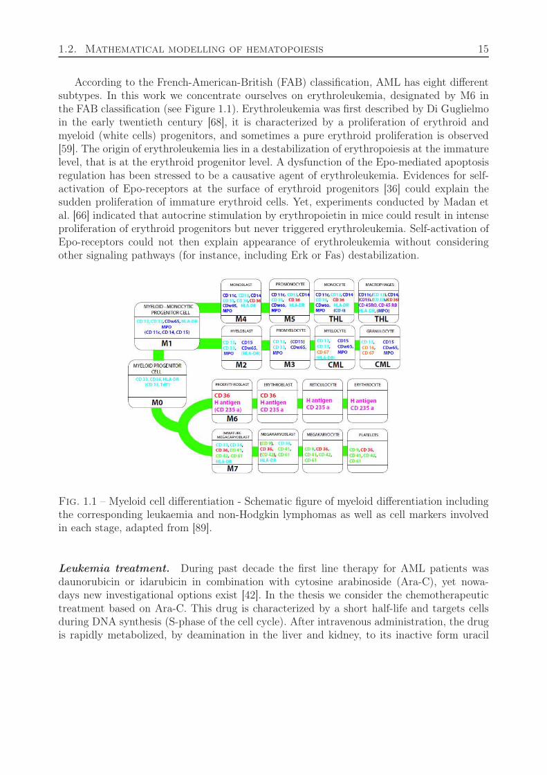
According to the French-American-British (FAB) classification, AML has eight differentsubtypes. In this work we concentrate ourselves on erythroleukemia, designated by M6 inthe FAB classification (see Figure 1.1). Erythroleukemia was first described by Di Guglielmoin the early twentieth century [68], it is characterized by a proliferation of erythroid andmyeloid (white cells) progenitors, and sometimes a pure erythroid proliferation is observed[59]. The origin of erythroleukemia lies in a destabilization of erythropoiesis at the immaturelevel, that is at the erythroid progenitor level. A dysfunction of the Epo-mediated apoptosisregulation has been stressed to be a causative agent of erythroleukemia. Evidences for self-activation of Epo-receptors at the surface of erythroid progenitors [36] could explain thesudden proliferation of immature erythroid cells. Yet, experiments conducted by Madan etal. [66] indicated that autocrine stimulation by erythropoietin in mice could result in intenseproliferation of erythroid progenitors but never triggered erythroleukemia. Self-activation ofEpo-receptors could not then explain appearance of erythroleukemia without consideringother signaling pathways (for instance, including Erk or Fas) destabilization.

Fig. 1.1 – Myeloid cell differentiation - Schematic figure of myeloid differentiation includingthe corresponding leukaemia and non-Hodgkin lymphomas as well as cell markers involvedin each stage, adapted from [89].

Leukemia treatment. During past decade the first line therapy for AML patients wasdaunorubicin or idarubicin in combination with cytosine arabinoside (Ara-C), yet nowa-days new investigational options exist [42]. In the thesis we consider the chemotherapeutictreatment based on Ara-C. This drug is characterized by a short half-life and targets cellsduring DNA synthesis (S-phase of the cell cycle). After intravenous administration, the drugis rapidly metabolized, by deamination in the liver and kidney, to its inactive form uracil

16

arabinoside (Ara-U). When in the bone marrow, it penetrates proliferating cells membraneand it can be transformed into its active form arabinoside triphosphate (Ara-CTP), whichparticipates in the DNA duplication, replacing natural nucleotides. When the proportion ofAra-CTP in the DNA becomes sufficiently high, the cell dies by apoptosis.

It is not always clear what dose of Ara-C should be administrated to each concretepatient to achieve the best efficacy. However, some standard protocol is usually applied. Thedesired therapeutic effect is to bring the disease into remission that means reappearanceof normal haemapoiesis with less than 5% blast cells in bone marrow. From 1980th thepharmacokinetics of high-dose Ara-C was studied [108]. Further clinical studies was needed todetermine the correct balance between efficacy an toxicity. Some trials were recently carriedout where authors showed [56] that the high-dose of Ara-C improve long-term disease control,but no differences between high-dose and standard-dose were found with regard to completeremission rates.

Ara-C acts on all proliferating cells whether they are leukemic or normal. Therefore,the aim in optimizing drug administration schedule is to increase cytotoxicity for leukemiccells and tolerance for normal cells. One possible approaches to this problem is based onchronotherapy, which takes into account the small differences in the temporal organisationof the cell cycle between normal and leukemic cells.

Chronotherapy. Chronotherapy signifies drug delivery synchronized with biological rhythmsin order to optimize the therapeutic outcomes. Cell physiology is regulated along the 24-htime [93]. The suprachiasmatic nucleus, a hypothalamic pacemaker clock and at least 12circadian genes act to generate and coordinate biological rhythms. The aim of anti-cancerchronomodulated treatment is to decrease toxicity and improve efficacy of the treatment. Thesame temporal pattern of phase-specific drug administration should have minimum cytotoxi-city toward population of normal cells and at the same time should show high cytotoxicitytoward cancer cells. It was shown that the survival rate of children with acute lymphoblasticleukemia (ALL) is greater for the evening schedule than for the morning one [92]. The cli-nical relevance of the chronotherapy principle was tested in large population of patient withmetastatic colorectal cancer [63, 64, 77]. Significant improvements in tolerability and anti-cancer efficacy were demonstrated in men, since women still displayed significantly toxicities.It means that the response of patients to chronotherapy can be heterogeneous and protocolshould be personalized to each patient or to subgroups of patients. Mathematical modelingis a good additional utility for that kind of research [9, 10].

Leukemia modeling. Mathematical modelling of leukemia has attracted much attentionsince the beginning of the 1970’s. In 1976, Rubinow and al. [97] proposed mathematicalmodel of acute myeloid leukemia where population of normal neutrophilic cells and leukemicmyeloblasts was considered as distinct but interacting populations. Dynamics of the numberof cells in each population was described by ordinary differential-difference equations takinginto account the age or maturity of cells. Cells of both population can be in the phase G0.Including the phase G0 was important to control the proliferation rate which depended on

1.2. Mathematical modelling of hematopoiesis 17

total number of cells. In the presence of leukemic cells, normal cells were destabilized andproduction of normal cells began to turn off. As a result, total population entirely consistedof leukemic cells and there were no normal cells. Mathematical models of chronic myeloidleukemia and cancer stem cells was proposed by F. Michor in [73, 74, 75]. Basing on [97]model Rubinow et al. [98] proposed a mathematical model of chemotherapeutic treatment ofacute myeloid leukemia. In order to model drug-treatment regime all cells, whether normalor leukemic, which are not in the resting phase G0, were subdivided into three compartmentsG1, S, G2+M according to their phase. It was assumed that 90 % of all cells in the phase Sin the moment of drug administration were killed. It was shown that even small changes inprotocol can have significant effects on the results of treatment. An optimal protocol of drugadministration was proposed. Another mathematical model of acute myeloid leukemia wassuggested in [3]. Populations of normal and leukemic cells were considered in the model. Twocell population dynamics followed a process of Gompertzian growth. Leukemic cells exhibitedinhibiting effect on the growth of the normal cells. The kinetic equations and steady-stateproperties of the model were described. A treatment model was proposed and numericallysimulated. It was shown that aggressive treatment of the disease with heavy doses of drugsis plausible. Very detailed description of PK/PD model of AML treatment with AraC wasproposed by P. F. Morrison and collaborators in [65, 78]. They introduced the model of drugdistribution and metabolism of AraC in the different parts of the organism and estimatedthe pharmacokinetic parameters for L1210 cell line (lymphocytic leukemia cells derived frommice). In the [65] authors carried out computer simulations of the treatment. A PK/PDmodel presented in this thesis is based on these works.

PK/PD modeling. With the development of mathematical modeling of cancer, pharmaco-kinetic-pharmacodynamic (PK/PD) models have received wide application. Pharmacodyna-mics is often summarized as the study of what a drug does to the diseased organs and wholebody, whereas pharmacokinetics is the study of what the body does to a drug and providesa metabolism scheme of drug transformation of its active form. PK/PD approach answerssuch important questions as (i) if the right drug has been selected and (ii) if the optimaldosage regimen has been established.

PK/PD modeling approach developed by Veng-Pedersen and co-workers [30, 117] dealswith stress erythropoiesis. Such approaches are usually centered on parameter estimationand model fitting to data (statistical approaches). S. Chapel et al. investigated the reticu-locyte response resulting from phlebotomy-induced erythropoietin (EPO) in adult sheep bymeans of PK/PD modeling [30]. This study was extended in the subsequent article [117]by considering the hemoglobin data to identify the relevant parameters of the cellular ki-netics of erythropoiesis in acute anemia and showed a good agreement with the observeddata. PK/PD model of the erythropoietic responses to single i.v. and s.c. (subcutaneous)administration of recombinant human erythropoietin (rHuEPO) in rats was studied in [123].A two-compartment pharmacokinetic model of rHuEPO involving linear first-order elimina-tion and Michaelis-Menten saturable kinetics after i.v. administration was used. In order todescribe s.c. administration the absorbtion kinetics is assumed. Proposed pharmacodynamic

18

model was based on combination of cell production and loss model and of indirect responsemodel. Several types of cells were considered among them earliest progenitor cells, which,in turn, converted to erythroblasts, reticulocytes and red blood cells. Indirect response mo-del was considered trough stimulation of responses by rHuEPO. In another article of S.Woo [124], a physiology-based PD model was developed in order to describe progression ofanemia caused by carboplatin in rats. A three-compartment PK model with plasma concen-tration and amounts of carboplatin in peripheral tissue was presented. The PD model forcarboplatin-induced anemia that include erythroid progenitors, erythroblasts, reticulocytesand mature red blood cells with taking into account stimulation through EPO concentrationwas considered. Such models could give an assess to optimization of erythropoietic treatmentof anemia.

1.3 Summary of the results

This dissertation is devoted to the development of hybrid models of cell population dyna-mics. It is applied to study hematopoiesis and blood disorders, such as anemia and leukemia.

The thesis contains four chapters. In the first chapter we present the description of themethod developed in this work and model examples of particle dynamics. In the secondchapter, a hybrid model of erythropoiesis is suggested and studied. The third chapter isdevoted to PK/PD modeling of leukemia treatment with AraC. In the last chapter thepassage from a hybrid model to a continuous model in the 1D case is investigated.

1.3.1 Hybrid Method

Cell populations represent complex multi-level systems where different levels (intracellu-lar, cellular, tissue, organism) interact with each other providing normal functioning of thewhole system. We introduce and study a hybrid model with off-lattice cell dynamics whichdescribe biological processes different levels.

Cells are considered as discrete objects. They can interact with each other and with thesurrounding medium mechanically and biochemically, they can divide, differentiate and diedue to apoptosis. Cell behavior is determined by intracellular regulatory networks describedby ordinary differential equations and by extracellular bio-chemical substances described bypartial differential equations. Each cell has ability of growing, moving, dividing and exchan-ging biochemical substances with surrounding medium. We describe motion of each cell bythe displacement of its center by Newton’s second law.

For each particular application intracellular and extracellular regulation should be spe-cified for each cell type as well as how cell fate (proliferation, differentiation and apoptosis)depends on regulatory networks. In this thesis the approach discussed above is applied tomulti-scale modelling of normal and leukaemic erythropoiesis.

1D hybrid models. We consider a hybrid model for multi-scale modelling of cells popu-lation. We start with the 1D case and study three model problems. In the first one, each cell

1.3. Summary of the results 19

can self-renew or die by apoptosis. In the second model, the case where cells self-renew ordifferentiate into another type of cells is studied. In the last model, we investigate the casewhere cells can divide or be in a quiescent state. Finally, we illustrate application of thesemodels to bacteria filament.

The fate of each cell in considered models is determined by intracellular and extracellularregulation. In the first (second) model we suppose that cell division and death (differentia-tion) are determined by some bio-chemical substances produced by the cells themselves. Weconsider the case where there are two such substances, u and v, which influence cell divisionand death. We come to the following system of equations :

⎧⎨⎩

dudt

= d1∂2u∂x2 + b1c − q1u,

dvdt

= d2∂2v∂x2 + b2c − q2v.

(1.1)

These equations describe the evolution of the extracellular concentrations u and v withtheir diffusion, production terms proportional to the concentration of cells c and with thedegradation term. We consider the no-flux boundary conditions.

Intracellular concentrations ui and vi in the i-th cell are described by the equations :

⎧⎨⎩

dui

dt= k

(1)1 u(x, t) − k

(1)2 ui(t) + H1,

dvi

dt= k

(2)1 v(x, t) − k

(2)2 vi(t) + H2.

(1.2)

The first term in the right-hand side of the first equation shows that the intracellular concen-tration ui grows proportionally to the value of the extracellular concentration u(x, t) at thespace point xi where the cell is located. In the first and second studied models the intra-cellular concentration of ui controls cell division while the concentration of vi controls celldeath (first model) and differentiation (second model).

In the third model we suppose that cells can be either in quiescent state or in cell cycle.When a cell enters cell cycle, it grows and then divides into two identical to itself cells.Extracellular regulation is described by system of partial differential equations. Intracellularregulatory networks is described by system of ordinary differential equations.

For each model pattern formation due to different values of parameters is studied anddiscussed. Extension of the first model where cells can either divide or die to 2D case wascarried out.

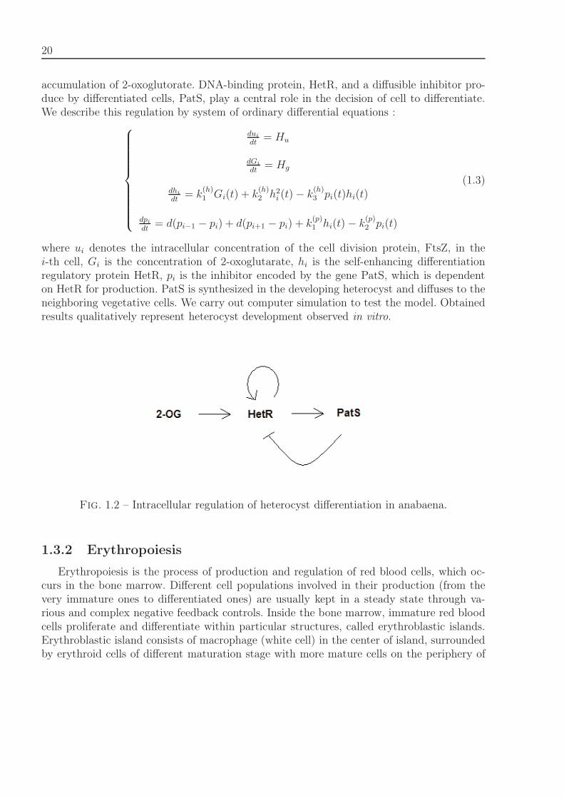
Bacteria filament growth. The filamentous cyanobacterium Anabaena sp. PCC 7120represents a chain of cells connected to each other and is a good model to study cell dif-ferentiation and pattern formation. Due to nitrogen starvation 5-10% of cells differentiateinto heterocytes, cells that fix nitrogen. This process is regulated by different internal andexternal signals. The intracellular regulation which determines cell differentiation is shownin Figure 1.2, [101]. Cell division is initiated by protein FtsZ, cell differentiation starts with

20

accumulation of 2-oxoglutorate. DNA-binding protein, HetR, and a diffusible inhibitor pro-duce by differentiated cells, PatS, play a central role in the decision of cell to differentiate.We describe this regulation by system of ordinary differential equations :⎧⎪⎪⎪⎪⎪⎪⎪⎪⎪⎨

⎪⎪⎪⎪⎪⎪⎪⎪⎪⎩

dui

dt= Hu

dGi

dt= Hg

dhi

dt= k

(h)1 Gi(t) + k

(h)2 h2

i (t) − k(h)3 pi(t)hi(t)

dpi

dt= d(pi−1 − pi) + d(pi+1 − pi) + k

(p)1 hi(t) − k

(p)2 pi(t)

(1.3)

where ui denotes the intracellular concentration of the cell division protein, FtsZ, in thei-th cell, Gi is the concentration of 2-oxoglutarate, hi is the self-enhancing differentiationregulatory protein HetR, pi is the inhibitor encoded by the gene PatS, which is dependenton HetR for production. PatS is synthesized in the developing heterocyst and diffuses to theneighboring vegetative cells. We carry out computer simulation to test the model. Obtainedresults qualitatively represent heterocyst development observed in vitro.

Fig. 1.2 – Intracellular regulation of heterocyst differentiation in anabaena.

1.3.2 Erythropoiesis

Erythropoiesis is the process of production and regulation of red blood cells, which oc-curs in the bone marrow. Different cell populations involved in their production (from thevery immature ones to differentiated ones) are usually kept in a steady state through va-rious and complex negative feedback controls. Inside the bone marrow, immature red bloodcells proliferate and differentiate within particular structures, called erythroblastic islands.Erythroblastic island consists of macrophage (white cell) in the center of island, surroundedby erythroid cells of different maturation stage with more mature cells on the periphery of

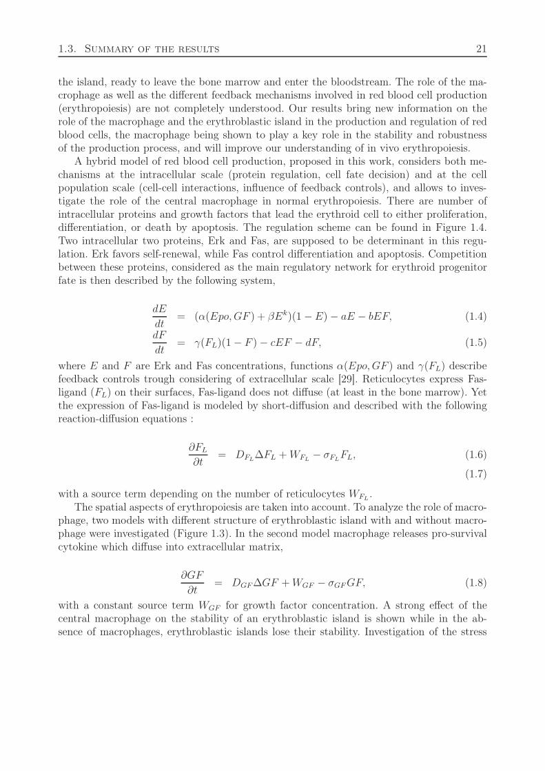
1.3. Summary of the results 21

the island, ready to leave the bone marrow and enter the bloodstream. The role of the ma-crophage as well as the different feedback mechanisms involved in red blood cell production(erythropoiesis) are not completely understood. Our results bring new information on therole of the macrophage and the erythroblastic island in the production and regulation of redblood cells, the macrophage being shown to play a key role in the stability and robustnessof the production process, and will improve our understanding of in vivo erythropoiesis.

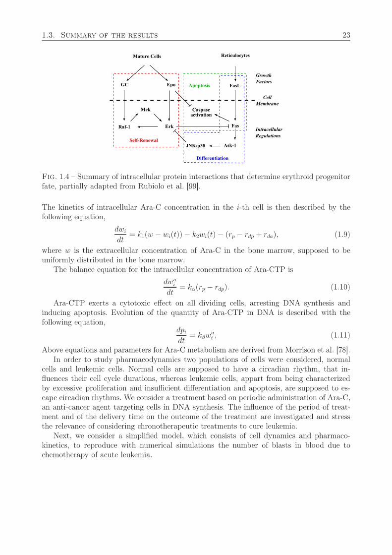
A hybrid model of red blood cell production, proposed in this work, considers both me-chanisms at the intracellular scale (protein regulation, cell fate decision) and at the cellpopulation scale (cell-cell interactions, influence of feedback controls), and allows to inves-tigate the role of the central macrophage in normal erythropoiesis. There are number ofintracellular proteins and growth factors that lead the erythroid cell to either proliferation,differentiation, or death by apoptosis. The regulation scheme can be found in Figure 1.4.Two intracellular two proteins, Erk and Fas, are supposed to be determinant in this regu-lation. Erk favors self-renewal, while Fas control differentiation and apoptosis. Competitionbetween these proteins, considered as the main regulatory network for erythroid progenitorfate is then described by the following system,

dE

dt= (α(Epo, GF ) + βEk)(1 − E) − aE − bEF, (1.4)

dF

dt= γ(FL)(1 − F ) − cEF − dF, (1.5)

where E and F are Erk and Fas concentrations, functions α(Epo, GF ) and γ(FL) describefeedback controls trough considering of extracellular scale [29]. Reticulocytes express Fas-ligand (FL) on their surfaces, Fas-ligand does not diffuse (at least in the bone marrow). Yetthe expression of Fas-ligand is modeled by short-diffusion and described with the followingreaction-diffusion equations :

∂FL

∂t= DFL

ΔFL + WFL− σFL

FL, (1.6)

(1.7)

with a source term depending on the number of reticulocytes WFL.

The spatial aspects of erythropoiesis are taken into account. To analyze the role of macro-phage, two models with different structure of erythroblastic island with and without macro-phage were investigated (Figure 1.3). In the second model macrophage releases pro-survivalcytokine which diffuse into extracellular matrix,

∂GF

∂t= DGF ΔGF + WGF − σGF GF, (1.8)

with a constant source term WGF for growth factor concentration. A strong effect of thecentral macrophage on the stability of an erythroblastic island is shown while in the ab-sence of macrophages, erythroblastic islands lose their stability. Investigation of the stress

22

erythropoiesis model concludes that stability does not decrease responsiveness of the model.Comparison of modelling with experiments on anemia in mice is carried out.

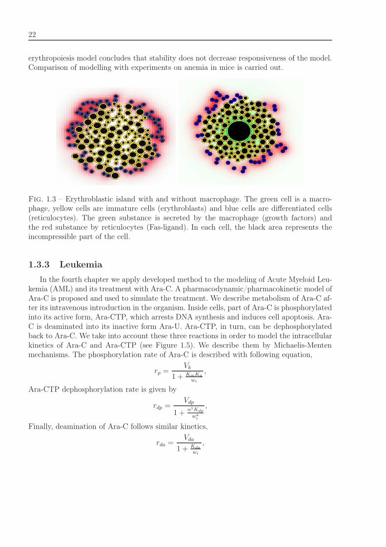
Fig. 1.3 – Erythroblastic island with and without macrophage. The green cell is a macro-phage, yellow cells are immature cells (erythroblasts) and blue cells are differentiated cells(reticulocytes). The green substance is secreted by the macrophage (growth factors) andthe red substance by reticulocytes (Fas-ligand). In each cell, the black area represents theincompressible part of the cell.

1.3.3 Leukemia

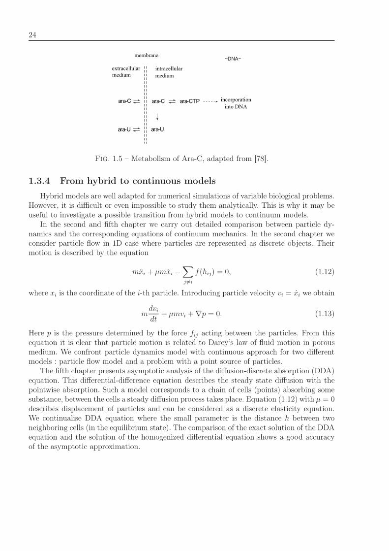
In the fourth chapter we apply developed method to the modeling of Acute Myeloid Leu-kemia (AML) and its treatment with Ara-C. A pharmacodynamic/pharmacokinetic model ofAra-C is proposed and used to simulate the treatment. We describe metabolism of Ara-C af-ter its intravenous introduction in the organism. Inside cells, part of Ara-C is phosphorylatedinto its active form, Ara-CTP, which arrests DNA synthesis and induces cell apoptosis. Ara-C is deaminated into its inactive form Ara-U. Ara-CTP, in turn, can be dephosphorylatedback to Ara-C. We take into account these three reactions in order to model the intracellularkinetics of Ara-C and Ara-CTP (see Figure 1.5). We describe them by Michaelis-Mentenmechanisms. The phosphorylation rate of Ara-C is described with following equation,

rp =Vk

1 + KmKa

wi

,

Ara-CTP dephosphorylation rate is given by

rdp =Vdp

1 +α1Kdp

wai

,

Finally, deamination of Ara-C follows similar kinetics,

rda =Vda

1 + Kda

wi

,

1.3. Summary of the results 23

GrowthFactors

Cell Membrane

Intracellular Regulations

Fig. 1.4 – Summary of intracellular protein interactions that determine erythroid progenitorfate, partially adapted from Rubiolo et al. [99].

The kinetics of intracellular Ara-C concentration in the i-th cell is then described by thefollowing equation,

dwi

dt= k1(w − wi(t)) − k2wi(t) − (rp − rdp + rda), (1.9)

where w is the extracellular concentration of Ara-C in the bone marrow, supposed to beuniformly distributed in the bone marrow.

The balance equation for the intracellular concentration of Ara-CTP is

dwai

dt= kα(rp − rdp). (1.10)

Ara-CTP exerts a cytotoxic effect on all dividing cells, arresting DNA synthesis andinducing apoptosis. Evolution of the quantity of Ara-CTP in DNA is described with thefollowing equation,

dpi

dt= kβwa

i , (1.11)

Above equations and parameters for Ara-C metabolism are derived from Morrison et al. [78].In order to study pharmacodynamics two populations of cells were considered, normal

cells and leukemic cells. Normal cells are supposed to have a circadian rhythm, that in-fluences their cell cycle durations, whereas leukemic cells, appart from being characterizedby excessive proliferation and insufficient differentiation and apoptosis, are supposed to es-cape circadian rhythms. We consider a treatment based on periodic administration of Ara-C,an anti-cancer agent targeting cells in DNA synthesis. The influence of the period of treat-ment and of the delivery time on the outcome of the treatment are investigated and stressthe relevance of considering chronotherapeutic treatments to cure leukemia.

Next, we consider a simplified model, which consists of cell dynamics and pharmaco-kinetics, to reproduce with numerical simulations the number of blasts in blood due tochemotherapy of acute leukemia.

24

incorporation into DNA

intracellular medium

extracellular

membrane

ara-C ara-C

ara-U ara-U

ara-CTP

medium

Fig. 1.5 – Metabolism of Ara-C, adapted from [78].

1.3.4 From hybrid to continuous models

Hybrid models are well adapted for numerical simulations of variable biological problems.However, it is difficult or even impossible to study them analytically. This is why it may beuseful to investigate a possible transition from hybrid models to continuum models.

In the second and fifth chapter we carry out detailed comparison between particle dy-namics and the corresponding equations of continuum mechanics. In the second chapter weconsider particle flow in 1D case where particles are represented as discrete objects. Theirmotion is described by the equation

mxi + μmxi −∑j �=i

f(hij) = 0, (1.12)

where xi is the coordinate of the i-th particle. Introducing particle velocity vi = xi we obtain

mdvi

dt+ μmvi + ∇p = 0. (1.13)

Here p is the pressure determined by the force fij acting between the particles. From thisequation it is clear that particle motion is related to Darcy’s law of fluid motion in porousmedium. We confront particle dynamics model with continuous approach for two differentmodels : particle flow model and a problem with a point source of particles.

The fifth chapter presents asymptotic analysis of the diffusion-discrete absorption (DDA)equation. This differential-difference equation describes the steady state diffusion with thepointwise absorption. Such a model corresponds to a chain of cells (points) absorbing somesubstance, between the cells a steady diffusion process takes place. Equation (1.12) with μ = 0describes displacement of particles and can be considered as a discrete elasticity equation.We continualise DDA equation where the small parameter is the distance h between twoneighboring cells (in the equilibrium state). The comparison of the exact solution of the DDAequation and the solution of the homogenized differential equation shows a good accuracyof the asymptotic approximation.

25

Chapitre 2

Hybrid method and model examples

2.1 Method description

In this thesis we introduce and study a hybrid model with off-lattice cell dynamics. Cellscan interact with each other and with the surrounding medium mechanically and bioche-mically, they can divide, differentiate and die due to apoptosis. Cell behavior is determinedby intracellular regulatory networks described by ordinary differential equations and by ex-tracellular bio-chemical substances described by partial differential equations. Each cell hasability of growing, moving, dividing and exchanging biochemical substances with surroundingmedium.

In order to describe mechanical interaction between cells, we restrict ourselves here to thesimplest model where cells are represented as elastic balls. Consider two elastic balls withthe centers at the points x1 and x2 and with the radii, respectively, r1 and r2. If the distanceh12 between the centers is less then the sum of the radii, r1 + r2, then there is a repulsiveforce between them f12 which depends on the distance h12 (Figure 2.2 (left)). If a particlewith the center at xi is surrounded by several other particles with the centers at the pointsxj , j = 1, ..., k, then we consider the pairwise forces fij assuming that they are independentof each other. This assumption corresponds to small deformation of the particles. Hence, wefind the total force Fi acting on the i-th particle from all other particles, Fi =

∑j �=i fij. The

motion of the particles can now be described as the motion of their centers by Newton’ssecond law

mxi + μmx −∑j �=i

f(hij) = 0, (2.1)

where m is the mass of the particle, the second term in the left-hand side describes thefriction by the surrounding medium, the third term is the potential force between cells. Weconsider the force between particles in the following form

fij =

{K

h0−hij

hij−(h0−h1), h0 − h1 < hij < h0

0, hij ≥ h0

(2.2)

26

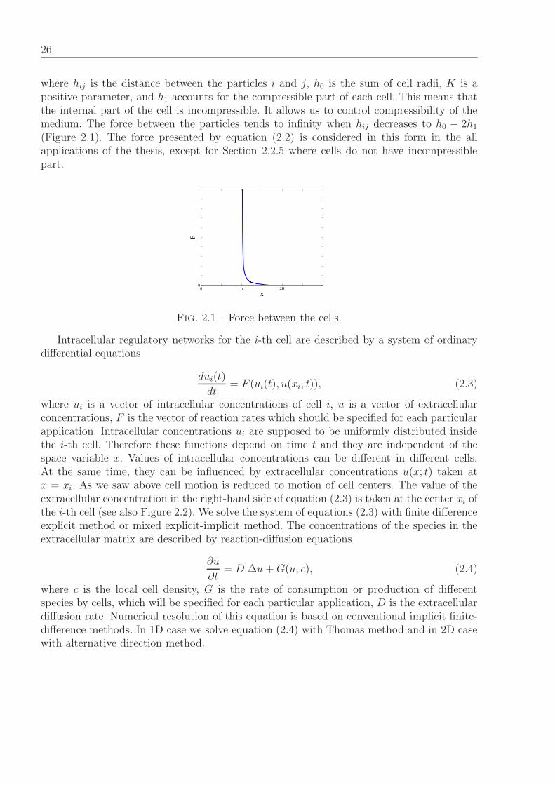
where hij is the distance between the particles i and j, h0 is the sum of cell radii, K is apositive parameter, and h1 accounts for the compressible part of each cell. This means thatthe internal part of the cell is incompressible. It allows us to control compressibility of themedium. The force between the particles tends to infinity when hij decreases to h0 − 2h1

(Figure 2.1). The force presented by equation (2.2) is considered in this form in the allapplications of the thesis, except for Section 2.2.5 where cells do not have incompressiblepart.

0 h 2R0

x

F

Fig. 2.1 – Force between the cells.

Intracellular regulatory networks for the i-th cell are described by a system of ordinarydifferential equations

dui(t)

dt= F (ui(t), u(xi, t)), (2.3)

where ui is a vector of intracellular concentrations of cell i, u is a vector of extracellularconcentrations, F is the vector of reaction rates which should be specified for each particularapplication. Intracellular concentrations ui are supposed to be uniformly distributed insidethe i-th cell. Therefore these functions depend on time t and they are independent of thespace variable x. Values of intracellular concentrations can be different in different cells.At the same time, they can be influenced by extracellular concentrations u(x; t) taken atx = xi. As we saw above cell motion is reduced to motion of cell centers. The value of theextracellular concentration in the right-hand side of equation (2.3) is taken at the center xi ofthe i-th cell (see also Figure 2.2). We solve the system of equations (2.3) with finite differenceexplicit method or mixed explicit-implicit method. The concentrations of the species in theextracellular matrix are described by reaction-diffusion equations

∂u

∂t= D Δu + G(u, c), (2.4)

where c is the local cell density, G is the rate of consumption or production of differentspecies by cells, which will be specified for each particular application, D is the extracellulardiffusion rate. Numerical resolution of this equation is based on conventional implicit finite-difference methods. In 1D case we solve equation (2.4) with Thomas method and in 2D casewith alternative direction method.

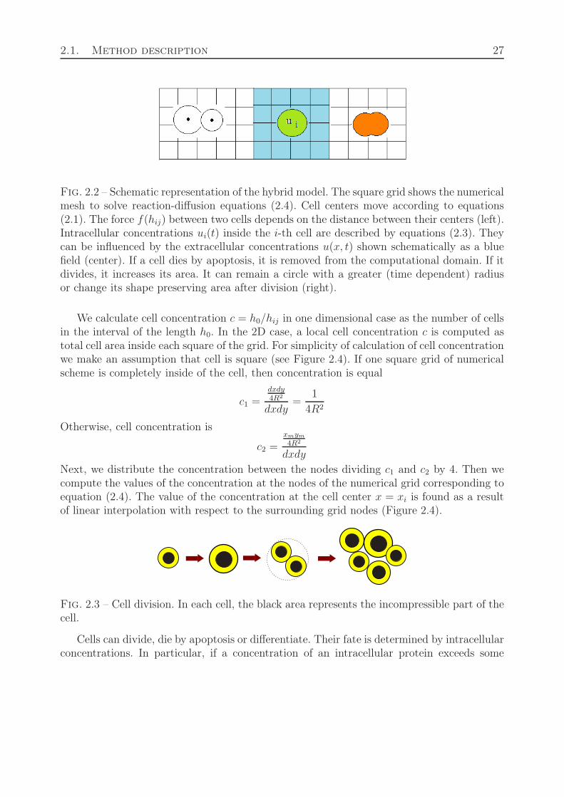
2.1. Method description 27

Fig. 2.2 – Schematic representation of the hybrid model. The square grid shows the numericalmesh to solve reaction-diffusion equations (2.4). Cell centers move according to equations(2.1). The force f(hij) between two cells depends on the distance between their centers (left).Intracellular concentrations ui(t) inside the i-th cell are described by equations (2.3). Theycan be influenced by the extracellular concentrations u(x, t) shown schematically as a bluefield (center). If a cell dies by apoptosis, it is removed from the computational domain. If itdivides, it increases its area. It can remain a circle with a greater (time dependent) radiusor change its shape preserving area after division (right).

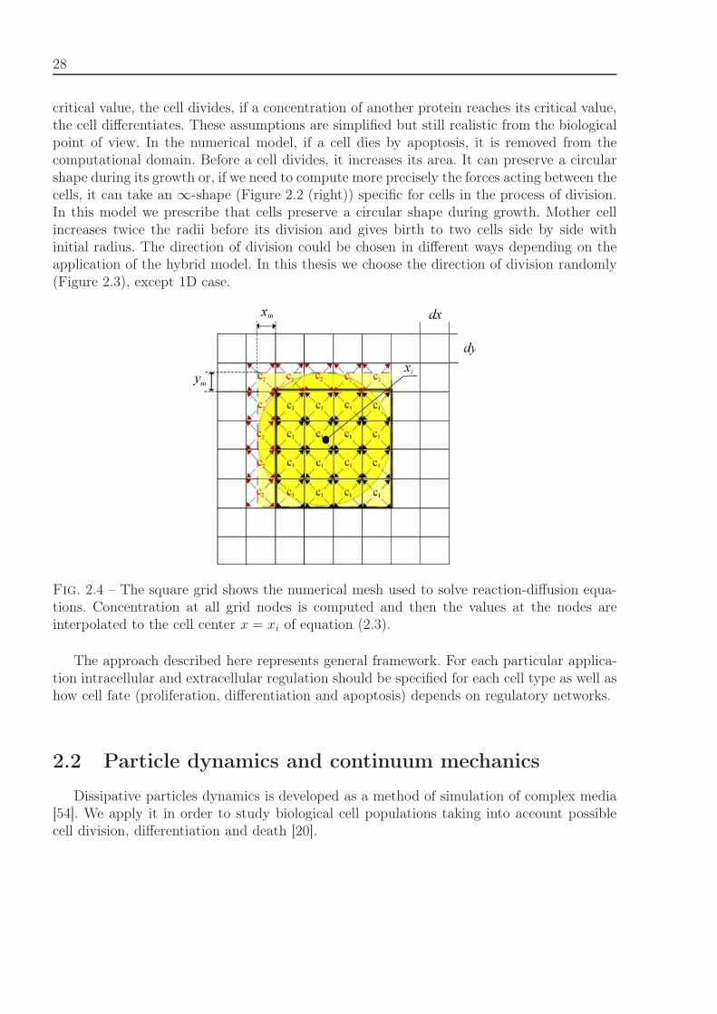
We calculate cell concentration c = h0/hij in one dimensional case as the number of cellsin the interval of the length h0. In the 2D case, a local cell concentration c is computed astotal cell area inside each square of the grid. For simplicity of calculation of cell concentrationwe make an assumption that cell is square (see Figure 2.4). If one square grid of numericalscheme is completely inside of the cell, then concentration is equal

c1 =dxdy4R2

dxdy=

1

4R2

Otherwise, cell concentration is

c2 =xmym

4R2

dxdy

Next, we distribute the concentration between the nodes dividing c1 and c2 by 4. Then wecompute the values of the concentration at the nodes of the numerical grid corresponding toequation (2.4). The value of the concentration at the cell center x = xi is found as a resultof linear interpolation with respect to the surrounding grid nodes (Figure 2.4).

Fig. 2.3 – Cell division. In each cell, the black area represents the incompressible part of thecell.

Cells can divide, die by apoptosis or differentiate. Their fate is determined by intracellularconcentrations. In particular, if a concentration of an intracellular protein exceeds some

28

critical value, the cell divides, if a concentration of another protein reaches its critical value,the cell differentiates. These assumptions are simplified but still realistic from the biologicalpoint of view. In the numerical model, if a cell dies by apoptosis, it is removed from thecomputational domain. Before a cell divides, it increases its area. It can preserve a circularshape during its growth or, if we need to compute more precisely the forces acting between thecells, it can take an ∞-shape (Figure 2.2 (right)) specific for cells in the process of division.In this model we prescribe that cells preserve a circular shape during growth. Mother cellincreases twice the radii before its division and gives birth to two cells side by side withinitial radius. The direction of division could be chosen in different ways depending on theapplication of the hybrid model. In this thesis we choose the direction of division randomly(Figure 2.3), except 1D case.

Fig. 2.4 – The square grid shows the numerical mesh used to solve reaction-diffusion equa-tions. Concentration at all grid nodes is computed and then the values at the nodes areinterpolated to the cell center x = xi of equation (2.3).

The approach described here represents general framework. For each particular applica-tion intracellular and extracellular regulation should be specified for each cell type as well ashow cell fate (proliferation, differentiation and apoptosis) depends on regulatory networks.

2.2 Particle dynamics and continuum mechanics

Dissipative particles dynamics is developed as a method of simulation of complex media[54]. We apply it in order to study biological cell populations taking into account possiblecell division, differentiation and death [20].

2.2. Particle dynamics and continuum mechanics 29

2.2.1 From cells to particle dynamics

Consider two elastic balls with the centers at the points x1 and x2 and with the radii,respectively, r1 and r2. If the distance h12 between the centers is less than the sum of theradii, r1 +r2, then there is a repulsive force between them f12 which depends on the distanceh12.

If a particle with the center at xi is surrounded by several other particles with the centersat the points xj , j = 1, ..., k, then we consider the pairwise forces fij assuming that theyare independent of each other. This assumption corresponds to small deformation of theparticles. Hence, we find the total force Fi acting on the i-th particle from all other particles,

Fi =∑j �=i

fij.

The motion of the particles can now be described as the motion of their centers.

2.2.2 Particles and discrete equations

Consider a system of N particles in the plane. Denote their coordinates by x1, ..., xn. Herexi is a two-component vector. Suppose that all particles have the same mass m and considerthe equation of motion of the i-th particles in the form

xi + μmxi +∑j �=i

fij = 0. (2.5)

The dot denotes the derivative with respect to time, xi is the particle acceleration, xi is itsspeed. The second term in the left-hand side of this equation describes dissipation due tofriction, the last term is the sum of forces acting on this particle from all other particles.

The force fij acting between the particles i and j can be expressed through the potential :fij = −m∇φ(|x − xj |)x=xi

. Then

xi + μxi + ∇(∑

j �=i

φ(|x− xj |))

x=xi

= 0, 1, ..., N. (2.6)

Consider a square grid with the mesh points xi and the step δx. Denote by si the squarewith the side 2 δx and the center at the point xi. Let xi1, ..., xik ∈ si. Let us introducevelocity and density at the grid points :

vi =1

k

k∑j=1

xij , ρi =k

|si| ,

where |si| = 4(δx)2 is the area of si. Then∑j

φ(|x − xj |) ≈∑m

φ(|x− xm|)ρm|sm| ≈ U(x),

30

where

U(x) =

∫φ(|x − x′|)ρ(x′)dx′.

Taking a sum of equations (2.6) with respect to the points inside si, we obtain the discreteequation

ρidvi

dt+ μρivi + ρi(∇U)i = 0, (2.7)

where we use the approximation 1k

∑kj=1 φ(|xj−xm|) ≈ φ(|xi−xm|). Averaged equation (2.7)

may not be equivalent to (2.6). Two particles xj , xk ∈ si with opposite velocities cancel in(2.7) but not in (2.6). They result in the momentum transfer and can be taken into accountin (2.7) by additional dissipative terms. In numerical simulations, the equivalence of theseequations can be provided if we take an average velocity with respect to some ensembles ofparticles.

2.2.3 Continuous model

Consider the continuous analogue of discrete equation (2.7)

ρdv

dt+ μρv + ρ(∇U) = 0. (2.8)

This equation of motion should be completed by the equation of mass conservation :

∂ρ

∂t+ ∇.(ρv) = 0. (2.9)

We can write equation (2.8) in the form

ρ(∂v

∂t+ v.∇v) + μρv + ∇p − U∇ρ = 0, (2.10)

where p is the pressure, p = ρU . This equation is nonlocal because the potential U containthe integral. Using the Taylor expansion of the density ρ(x′) around the point x and keepingthe terms up to the second order, we obtain

ρ(∂v

∂t+ v.∇v) + μρv + ∇p − KΔρ∇ρ = 0. (2.11)

The pressure in this equation is different in comparison with the previous one but we keepfor it the same notation. This equation does not contain the potential anymore. Therefore,we cannot express the pressure through it, and we need to complete system (2.9), (2.11) byan equation of state, p = p(ρ). In the case μ = 0 and K = 0, (2.11) is the Euleur equationand system (2.9), (2.11) becomes the classical model of gas dynamics.

2.2. Particle dynamics and continuum mechanics 31

2.2.4 Energy

Denote the left hand-side of equation (2.8) by J(x, t). We take a scalar product of thisvector with v and integrate over R

2 :

∫Jvdx =

1

2

∫ρ∂|v|2∂t

dx +1

2

∫(ρv,∇|v|2)dx + μ

∫ρ|v|2dx +

∫(ρv,∇U)dx =

1

2

d

dt

∫(ρ|v|2 + ρU)dx + μ

∫ρ|v|2dx.

We use here formal integration by parts, equation (2.9) and the equality∫∂ρ

∂tUdx =

1

2

d

dt

∫ ∫φ(|x− x′|)ρ(x, t)ρ(x′, t)dxdx′ =

1

2

d

dt

∫ρUdx.

From (2.8) we obtain

dE

dt= −μ

∫ρ|v|2dx, (2.12)

where E is the sum of the kinetic and potential energy of the system :

E =1

2

∫ρ|v|2dx +

1

2

∫ρUdx.

It follows from (2.12) that the total energy of the system decreases, its kinetic energy tendsto zero while the potential energy to some constant. Total energy can also be introduced forthe system of particles. Similar to the continuous case, it decreases with time.

2.2.5 1D model of particle flow

In the 1D case, the last term in the left-hand side of the equation (2.11) has the formKρ′ρ′′ and can be included in the pressure. In the stationary case, neglecting the inertialterms, we obtain from (2.9), (2.11) :

μρv + p′ = 0, ρv = q, (2.13)

where q is some constant. The force between two spherical particles is considered in the form

f(h) =

{k h0/h−1

2−h0/h, h0/2 < h < h0,

0 , h > h0

, (2.14)

where h is the distance between their centers, k and h0 are positive parameters. The forcebetween the particles tends to infinity when h decreases to h0/2. On the other hand, thisforce equals zero if h ≥ h0. Hence, every given particles interacts with at most one otherparticle from the left of it and another one from the right.

32

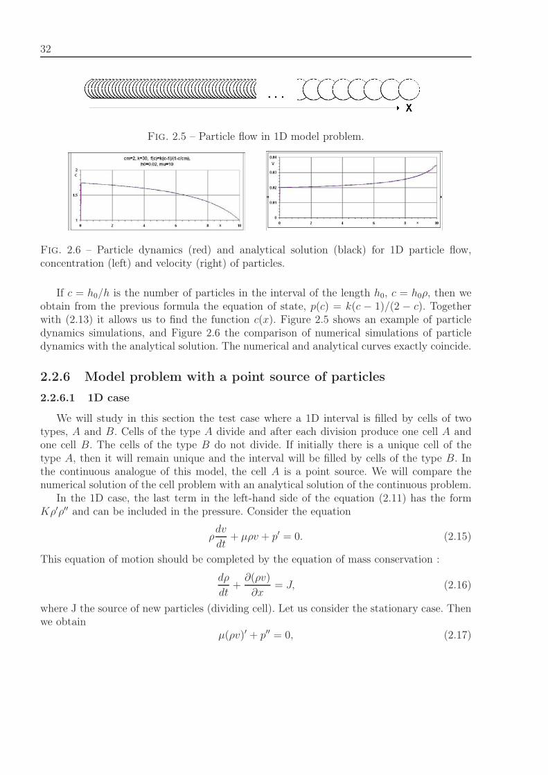
Fig. 2.5 – Particle flow in 1D model problem.

Fig. 2.6 – Particle dynamics (red) and analytical solution (black) for 1D particle flow,concentration (left) and velocity (right) of particles.

If c = h0/h is the number of particles in the interval of the length h0, c = h0ρ, then weobtain from the previous formula the equation of state, p(c) = k(c − 1)/(2 − c). Togetherwith (2.13) it allows us to find the function c(x). Figure 2.5 shows an example of particledynamics simulations, and Figure 2.6 the comparison of numerical simulations of particledynamics with the analytical solution. The numerical and analytical curves exactly coincide.

2.2.6 Model problem with a point source of particles

2.2.6.1 1D case

We will study in this section the test case where a 1D interval is filled by cells of twotypes, A and B. Cells of the type A divide and after each division produce one cell A andone cell B. The cells of the type B do not divide. If initially there is a unique cell of thetype A, then it will remain unique and the interval will be filled by cells of the type B. Inthe continuous analogue of this model, the cell A is a point source. We will compare thenumerical solution of the cell problem with an analytical solution of the continuous problem.

In the 1D case, the last term in the left-hand side of the equation (2.11) has the formKρ′ρ′′ and can be included in the pressure. Consider the equation

ρdv

dt+ μρv + p′ = 0. (2.15)

This equation of motion should be completed by the equation of mass conservation :

dρ

dt+

∂(ρv)

∂x= J, (2.16)

where J the source of new particles (dividing cell). Let us consider the stationary case. Thenwe obtain

μ(ρv)′ + p′′ = 0, (2.17)

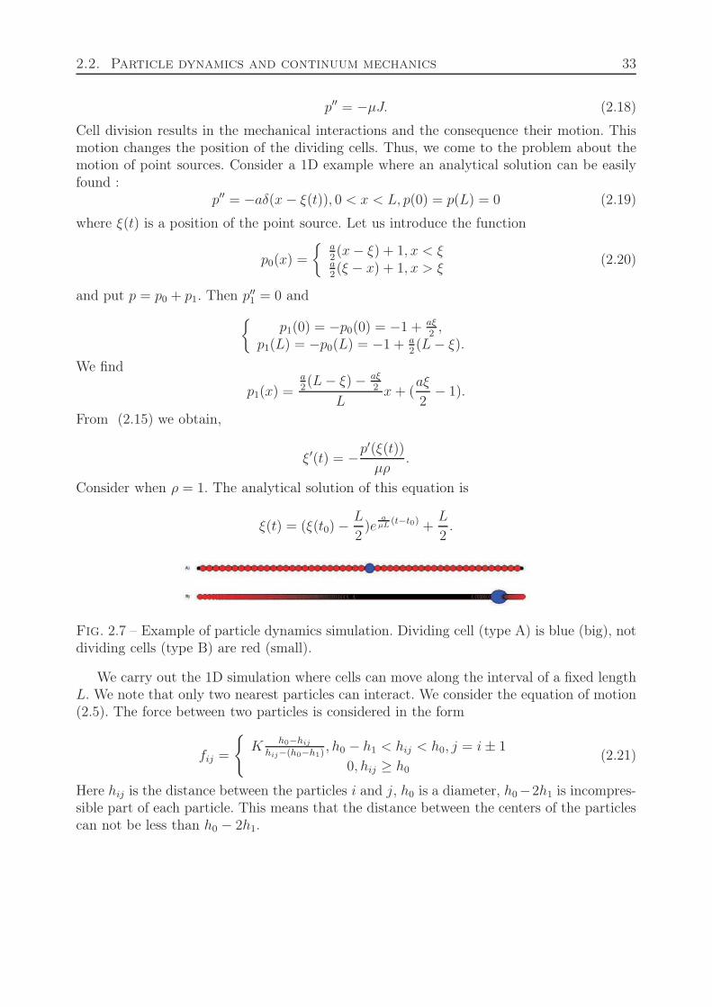
2.2. Particle dynamics and continuum mechanics 33

p′′ = −μJ. (2.18)

Cell division results in the mechanical interactions and the consequence their motion. Thismotion changes the position of the dividing cells. Thus, we come to the problem about themotion of point sources. Consider a 1D example where an analytical solution can be easilyfound :

p′′ = −aδ(x − ξ(t)), 0 < x < L, p(0) = p(L) = 0 (2.19)

where ξ(t) is a position of the point source. Let us introduce the function

p0(x) =

{a2(x − ξ) + 1, x < ξ

a2(ξ − x) + 1, x > ξ

(2.20)

and put p = p0 + p1. Then p′′1 = 0 and{p1(0) = −p0(0) = −1 + aξ

2,

p1(L) = −p0(L) = −1 + a2(L − ξ).

We find

p1(x) =a2(L − ξ) − aξ

2

Lx + (

aξ

2− 1).

From (2.15) we obtain,

ξ′(t) = −p′(ξ(t))μρ

.

Consider when ρ = 1. The analytical solution of this equation is

ξ(t) = (ξ(t0) − L

2)e

aμL

(t−t0) +L

2.

Fig. 2.7 – Example of particle dynamics simulation. Dividing cell (type A) is blue (big), notdividing cells (type B) are red (small).

We carry out the 1D simulation where cells can move along the interval of a fixed lengthL. We note that only two nearest particles can interact. We consider the equation of motion(2.5). The force between two particles is considered in the form

fij =

{K

h0−hij

hij−(h0−h1), h0 − h1 < hij < h0, j = i ± 1

0, hij ≥ h0

(2.21)

Here hij is the distance between the particles i and j, h0 is a diameter, h0−2h1 is incompres-sible part of each particle. This means that the distance between the centers of the particlescan not be less than h0 − 2h1.

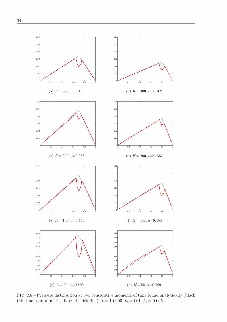
34

0 0.2 0.4 0.6 0.8 11

1.01

1.02

1.03

1.04

1.05

1.06

(a) K= 300, a=0.162

0 0.2 0.4 0.6 0.8 11

1.01

1.02

1.03

1.04

1.05

1.06

(b) K= 300, a=0.162

0 0.2 0.4 0.6 0.8 11

1.01

1.02

1.03

1.04

1.05

1.06

(c) K= 200, a=0.233

0 0.2 0.4 0.6 0.8 11

1.01

1.02

1.03

1.04

1.05

1.06

(d) K= 200, a=0.233

0 0.2 0.4 0.6 0.8 11

1.02

1.04

1.06

1.08

1.1

1.12

(e) K= 100, a=0.458

0 0.2 0.4 0.6 0.8 11

1.02

1.04

1.06

1.08

1.1

1.12

(f) K= 100, a=0.458

0 0.2 0.4 0.6 0.8 11

1.02

1.04

1.06

1.08

1.1

1.12

1.14

1.16

1.18

(g) K= 50, a=0.809

0 0.2 0.4 0.6 0.8 11

1.02

1.04

1.06

1.08

1.1

1.12

1.14

1.16

1.18

(h) K= 50, a=0.809

Fig. 2.8 – Pressure distribution at two consecutive moments of time found analytically (blackthin line) and numerically (red thick line) ; μ= 10 000, h0=0.01, h1= 0.005.

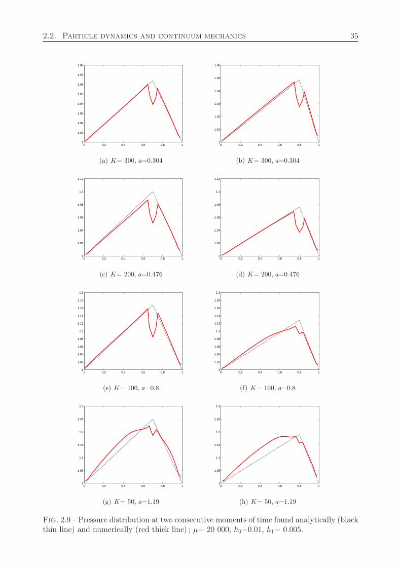
2.2. Particle dynamics and continuum mechanics 35

0 0.2 0.4 0.6 0.8 11

1.01

1.02

1.03

1.04

1.05

1.06

1.07

1.08

(a) K= 300, a=0.304

0 0.2 0.4 0.6 0.8 11

1.01

1.02

1.03

1.04

1.05

1.06

(b) K= 300, a=0.304

0 0.2 0.4 0.6 0.8 11

1.02

1.04

1.06

1.08

1.1

1.12

(c) K= 200, a=0.476

0 0.2 0.4 0.6 0.8 11

1.02

1.04

1.06

1.08

1.1

1.12

(d) K= 200, a=0.476

0 0.2 0.4 0.6 0.8 11

1.02

1.04

1.06

1.08

1.1

1.12

1.14

1.16

1.18

1.2

(e) K= 100, a=0.8

0 0.2 0.4 0.6 0.8 11

1.02

1.04

1.06

1.08

1.1

1.12

1.14

1.16

1.18

1.2

(f) K= 100, a=0.8

0 0.2 0.4 0.6 0.8 11

1.05

1.1

1.15

1.2

1.25

1.3

(g) K= 50, a=1.19

0 0.2 0.4 0.6 0.8 11

1.05

1.1

1.15

1.2

1.25

1.3

(h) K= 50, a=1.19

Fig. 2.9 – Pressure distribution at two consecutive moments of time found analytically (blackthin line) and numerically (red thick line) ; μ= 20 000, h0=0.01, h1= 0.005.

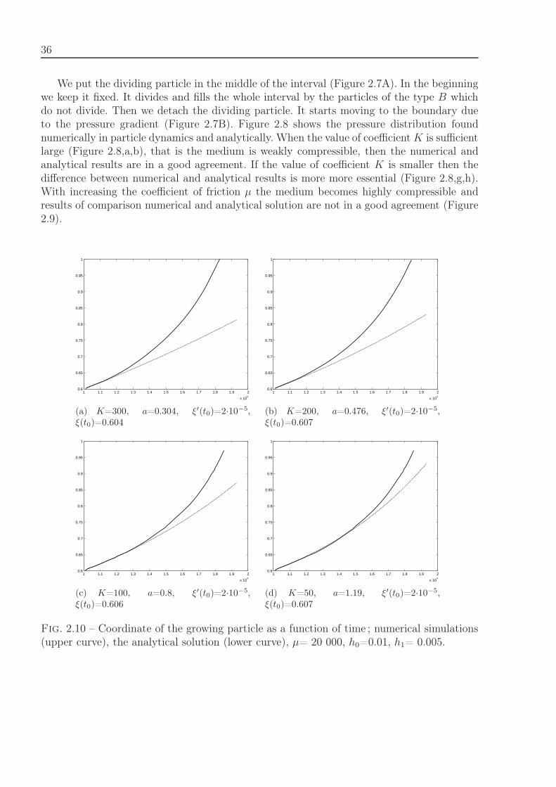
36

We put the dividing particle in the middle of the interval (Figure 2.7A). In the beginningwe keep it fixed. It divides and fills the whole interval by the particles of the type B whichdo not divide. Then we detach the dividing particle. It starts moving to the boundary dueto the pressure gradient (Figure 2.7B). Figure 2.8 shows the pressure distribution foundnumerically in particle dynamics and analytically. When the value of coefficient K is sufficientlarge (Figure 2.8,a,b), that is the medium is weakly compressible, then the numerical andanalytical results are in a good agreement. If the value of coefficient K is smaller then thedifference between numerical and analytical results is more more essential (Figure 2.8,g,h).With increasing the coefficient of friction μ the medium becomes highly compressible andresults of comparison numerical and analytical solution are not in a good agreement (Figure2.9).

1 1.1 1.2 1.3 1.4 1.5 1.6 1.7 1.8 1.9 2

x 104

0.6

0.65

0.7

0.75

0.8

0.85

0.9

0.95

1

(a) K=300, a=0.304, ξ′(t0)=2·10−5,ξ(t0)=0.604

1 1.1 1.2 1.3 1.4 1.5 1.6 1.7 1.8 1.9 2

x 104

0.6

0.65

0.7

0.75

0.8

0.85

0.9

0.95

1

(b) K=200, a=0.476, ξ′(t0)=2·10−5,ξ(t0)=0.607

1 1.1 1.2 1.3 1.4 1.5 1.6 1.7 1.8 1.9 2

x 104

0.6

0.65

0.7

0.75

0.8

0.85

0.9

0.95

1

(c) K=100, a=0.8, ξ′(t0)=2·10−5,ξ(t0)=0.606

1 1.1 1.2 1.3 1.4 1.5 1.6 1.7 1.8 1.9 2

x 104

0.6

0.65

0.7

0.75

0.8

0.85

0.9

0.95

1

(d) K=50, a=1.19, ξ′(t0)=2·10−5,ξ(t0)=0.607

Fig. 2.10 – Coordinate of the growing particle as a function of time ; numerical simulations(upper curve), the analytical solution (lower curve), μ= 20 000, h0=0.01, h1= 0.005.

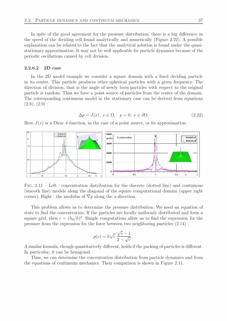
2.2. Particle dynamics and continuum mechanics 37

In spite of the good agreement for the pressure distribution, there is a big difference inthe speed of the dividing cell found analytically and numerically (Figure 2.22). A possibleexplanation can be related to the fact that the analytical solution is found under the quasi-stationary approximation. It may not be well applicable for particle dynamics because of theperiodic oscillations caused by cell division.

2.2.6.2 2D case

In the 2D model example we consider a square domain with a fixed dividing particlein its center. This particle produces other spherical particles with a given frequency. Thedirection of division, that is the angle of newly born particles with respect to the originalparticle is random. Thus we have a point source of particles from the center of the domain.The corresponding continuous model in the stationary case can be derived from equations(2.8), (2.9) :

Δp = J(x), x ∈ Ω, p = 0, x ∈ ∂Ω. (2.22)

Here J(x) is a Dirac δ-function, in the case of a point source, or its approximation.

Fig. 2.11 – Left : concentration distribution for the discrete (dotted line) and continuous(smooth line) models along the diagonal of the square computational domain (upper rightcorner). Right : the modulus of ∇p along the x-direction.

This problem allows us to determine the pressure distribution. We need an equation ofstate to find the concentration. If the particles are locally uniformly distributed and form asquare grid, then c = (h0/h)2. Simple computations allow us to find the expression for thepressure from the expression for the force between two neighboring particles (2.14) :

p(c) = k√

c

√c − 1

2 −√c

.

A similar formula, though quantitatively different, holds if the packing of particles is different.In particular, it can be hexagonal.

Thus, we can determine the concentration distribution from particle dynamics and fromthe equations of continuum mechanics. Their comparison is shown in Figure 2.11.

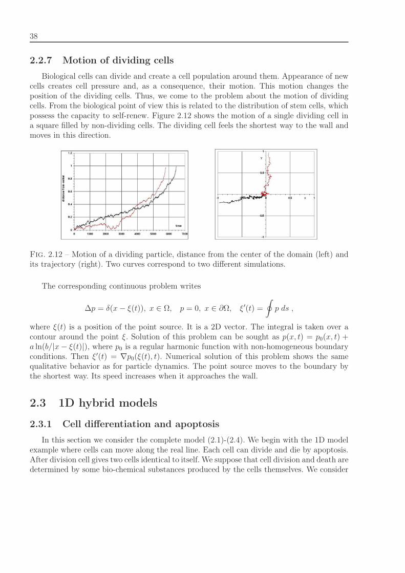
38

2.2.7 Motion of dividing cells

Biological cells can divide and create a cell population around them. Appearance of newcells creates cell pressure and, as a consequence, their motion. This motion changes theposition of the dividing cells. Thus, we come to the problem about the motion of dividingcells. From the biological point of view this is related to the distribution of stem cells, whichpossess the capacity to self-renew. Figure 2.12 shows the motion of a single dividing cell ina square filled by non-dividing cells. The dividing cell feels the shortest way to the wall andmoves in this direction.

Fig. 2.12 – Motion of a dividing particle, distance from the center of the domain (left) andits trajectory (right). Two curves correspond to two different simulations.

The corresponding continuous problem writes

Δp = δ(x − ξ(t)), x ∈ Ω, p = 0, x ∈ ∂Ω, ξ′(t) =

∮p ds ,

where ξ(t) is a position of the point source. It is a 2D vector. The integral is taken over acontour around the point ξ. Solution of this problem can be sought as p(x, t) = p0(x, t) +a ln(b/|x − ξ(t)|), where p0 is a regular harmonic function with non-homogeneous boundaryconditions. Then ξ′(t) = ∇p0(ξ(t), t). Numerical solution of this problem shows the samequalitative behavior as for particle dynamics. The point source moves to the boundary bythe shortest way. Its speed increases when it approaches the wall.

2.3 1D hybrid models

2.3.1 Cell differentiation and apoptosis

In this section we consider the complete model (2.1)-(2.4). We begin with the 1D modelexample where cells can move along the real line. Each cell can divide and die by apoptosis.After division cell gives two cells identical to itself. We suppose that cell division and death aredetermined by some bio-chemical substances produced by the cells themselves. We consider

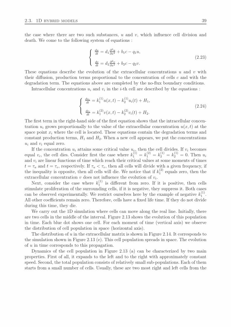
2.3. 1D hybrid models 39

the case where there are two such substances, u and v, which influence cell division anddeath. We come to the following system of equations :⎧⎨

⎩dudt

= d1∂2u∂x2 + b1c − q1u,

dvdt

= d2∂2v∂x2 + b2c − q2v.

(2.23)

These equations describe the evolution of the extracellular concentrations u and v withtheir diffusion, production terms proportional to the concentration of cells c and with thedegradation term. The equations above are completed by the no-flux boundary conditions.

Intracellular concentrations ui and vi in the i-th cell are described by the equations :⎧⎨⎩

dui

dt= k

(1)1 u(x, t) − k

(1)2 ui(t) + H1,

dvi

dt= k

(2)1 v(x, t) − k

(2)2 vi(t) + H2.

(2.24)

The first term in the right-hand side of the first equation shows that the intracellular concen-tration ui grows proportionally to the value of the extracellular concentration u(x, t) at thespace point xi where the cell is located. These equations contain the degradation terms andconstant production terms, H1 and H2. When a new cell appears, we put the concentrationsui and vi equal zero.

If the concentration ui attains some critical value uc, then the cell divides. If vi becomesequal vc, the cell dies. Consider first the case where k

(1)1 = k

(2)1 = k

(1)2 = k

(1)2 = 0. Then ui

and vi are linear functions of time which reach their critical values at some moments of timest = τu and t = τv, respectively. If τu < τv, then all cells will divide with a given frequency, ifthe inequality is opposite, then all cells will die. We notice that if k

(2)1 equals zero, then the

extracellular concentration v does not influence the evolution of vi.

Next, consider the case where k(1)1 is different from zero. If it is positive, then cells

stimulate proliferation of the surrounding cells, if it is negative, they suppress it. Both casescan be observed experimentally. We restrict ourselves here by the example of negative k

(1)1 .

All other coefficients remain zero. Therefore, cells have a fixed life time. If they do not divideduring this time, they die.

We carry out the 1D simulation where cells can move along the real line. Initially, thereare two cells in the middle of the interval. Figure 2.13 shows the evolution of this populationin time. Each blue dot shows one cell. For each moment of time (vertical axis) we observethe distribution of cell population in space (horizontal axis).

The distribution of u in the extracellular matrix is shown in Figure 2.14. It corresponds tothe simulation shown in Figure 2.13 (e). This cell population spreads in space. The evolutionof u in time corresponds to this propagation.

Dynamics of the cell population in Figure 2.13 (a) can be characterized by two mainproperties. First of all, it expands to the left and to the right with approximately constantspeed. Second, the total population consists of relatively small sub-populations. Each of themstarts from a small number of cells. Usually, these are two most right and left cells from the

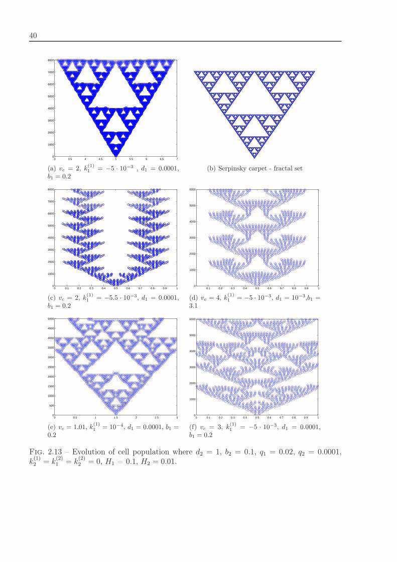
40

3 3.5 4 4.5 5 5.5 6 6.5 70

1000

2000

3000

4000

5000

6000

7000

8000

(a) vc = 2, k(1)1 = −5 · 10−3 , d1 = 0.0001,

b1 = 0.2(b) Serpinsky carpet - fractal set

0 0.1 0.2 0.3 0.4 0.5 0.6 0.7 0.8 0.9 10

1000

2000

3000

4000

5000

6000

7000

8000

(c) vc = 2, k(1)1 = −5.5 · 10−3, d1 = 0.0001,

b1 = 0.2

0.1 0.2 0.3 0.4 0.5 0.6 0.7 0.8 0.9 10

1000

2000

3000

4000

5000

6000

(d) vc = 4, k(1)1 = −5 · 10−3, d1 = 10−3,b1 =

3.1

0 0.5 1 1.5 2 2.5 30

500

1000

1500

2000

2500

3000

3500

4000

4500

5000

(e) vc = 1.01, k(1)1 = 10−4, d1 = 0.0001, b1 =

0.2

0 0.1 0.2 0.3 0.4 0.5 0.6 0.7 0.8 0.9 10

1000

2000

3000

4000

5000

6000

(f) vc = 3, k(1)1 = −5 · 10−3, d1 = 0.0001,

b1 = 0.2

Fig. 2.13 – Evolution of cell population where d2 = 1, b2 = 0.1, q1 = 0.02, q2 = 0.0001,k

(1)2 = k

(2)1 = k

(2)2 = 0, H1 = 0.1, H2 = 0.01.

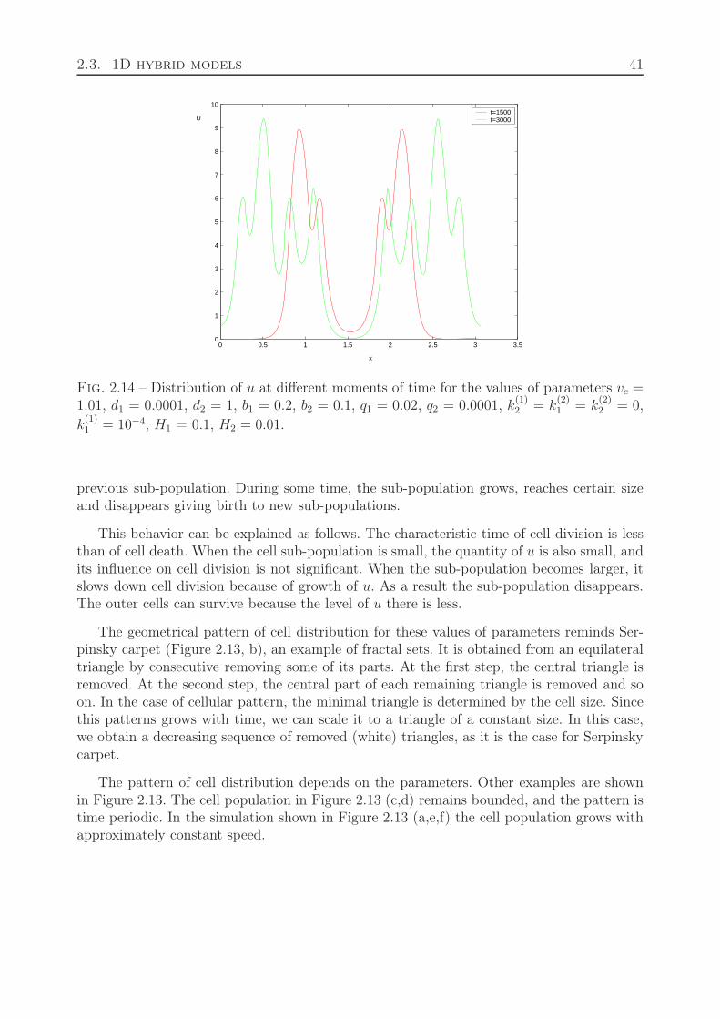
2.3. 1D hybrid models 41

0 0.5 1 1.5 2 2.5 3 3.50

1

2

3

4

5

6

7

8

9

10t=1500t=3000U

x

Fig. 2.14 – Distribution of u at different moments of time for the values of parameters vc =1.01, d1 = 0.0001, d2 = 1, b1 = 0.2, b2 = 0.1, q1 = 0.02, q2 = 0.0001, k

(1)2 = k

(2)1 = k

(2)2 = 0,

k(1)1 = 10−4, H1 = 0.1, H2 = 0.01.

previous sub-population. During some time, the sub-population grows, reaches certain sizeand disappears giving birth to new sub-populations.

This behavior can be explained as follows. The characteristic time of cell division is lessthan of cell death. When the cell sub-population is small, the quantity of u is also small, andits influence on cell division is not significant. When the sub-population becomes larger, itslows down cell division because of growth of u. As a result the sub-population disappears.The outer cells can survive because the level of u there is less.

The geometrical pattern of cell distribution for these values of parameters reminds Ser-pinsky carpet (Figure 2.13, b), an example of fractal sets. It is obtained from an equilateraltriangle by consecutive removing some of its parts. At the first step, the central triangle isremoved. At the second step, the central part of each remaining triangle is removed and soon. In the case of cellular pattern, the minimal triangle is determined by the cell size. Sincethis patterns grows with time, we can scale it to a triangle of a constant size. In this case,we obtain a decreasing sequence of removed (white) triangles, as it is the case for Serpinskycarpet.

The pattern of cell distribution depends on the parameters. Other examples are shownin Figure 2.13. The cell population in Figure 2.13 (c,d) remains bounded, and the pattern istime periodic. In the simulation shown in Figure 2.13 (a,e,f) the cell population grows withapproximately constant speed.

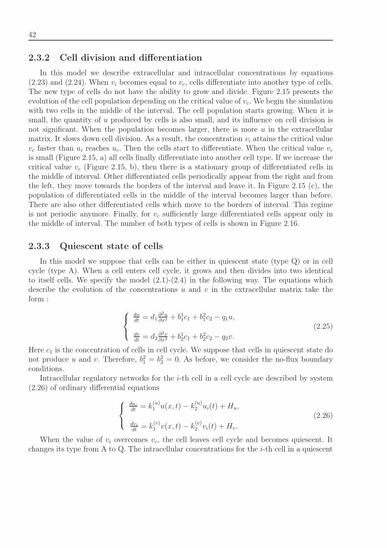
42

2.3.2 Cell division and differentiation

In this model we describe extracellular and intracellular concentrations by equations(2.23) and (2.24). When vi becomes equal to vc, cells differentiate into another type of cells.The new type of cells do not have the ability to grow and divide. Figure 2.15 presents theevolution of the cell population depending on the critical value of vc. We begin the simulationwith two cells in the middle of the interval. The cell population starts growing. When it issmall, the quantity of u produced by cells is also small, and its influence on cell division isnot significant. When the population becomes larger, there is more u in the extracellularmatrix. It slows down cell division. As a result, the concentration vi attains the critical valuevc faster than ui reaches uc. Then the cells start to differentiate. When the critical value vc

is small (Figure 2.15, a) all cells finally differentiate into another cell type. If we increase thecritical value vc (Figure 2.15, b), then there is a stationary group of differentiated cells inthe middle of interval. Other differentiated cells periodically appear from the right and fromthe left, they move towards the borders of the interval and leave it. In Figure 2.15 (c), thepopulation of differentiated cells in the middle of the interval becomes larger than before.There are also other differentiated cells which move to the borders of interval. This regimeis not periodic anymore. Finally, for vc sufficiently large differentiated cells appear only inthe middle of interval. The number of both types of cells is shown in Figure 2.16.

2.3.3 Quiescent state of cells

In this model we suppose that cells can be either in quiescent state (type Q) or in cellcycle (type A). When a cell enters cell cycle, it grows and then divides into two identicalto itself cells. We specify the model (2.1)-(2.4) in the following way. The equations whichdescribe the evolution of the concentrations u and v in the extracellular matrix take theform : ⎧⎨

⎩dudt

= d1∂2u∂x2 + b1

1c1 + b21c2 − q1u,

dvdt

= d2∂2v∂x2 + b1

2c1 + b22c2 − q2v.

(2.25)

Here c1 is the concentration of cells in cell cycle. We suppose that cells in quiescent state donot produce u and v. Therefore, b2

1 = b22 = 0. As before, we consider the no-flux boundary

conditions.Intracellular regulatory networks for the i-th cell in a cell cycle are described by system

(2.26) of ordinary differential equations⎧⎨⎩

dui

dt= k

(u)1 u(x, t) − k

(u)2 ui(t) + Hu,

dvi

dt= k

(v)1 v(x, t) − k

(v)2 vi(t) + Hv.

(2.26)

When the value of vi overcomes vc, the cell leaves cell cycle and becomes quiescent. Itchanges its type from A to Q. The intracellular concentrations for the i-th cell in a quiescent

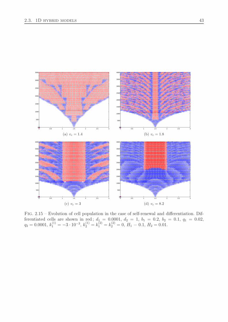
2.3. 1D hybrid models 43

0 0.5 1 1.5 2 2.5 30

500

1000

1500

2000

2500

3000

3500

(a) vc = 1.4

0 0.5 1 1.5 2 2.5 30

500

1000

1500

2000

2500

3000

3500

4000

(b) vc = 1.8

0 0.5 1 1.5 2 2.5 30

500

1000

1500

2000

2500

3000

3500

4000

(c) vc = 3

0 0.5 1 1.5 2 2.5 30

500

1000

1500

2000

2500

3000

3500

4000

(d) vc = 8.2

Fig. 2.15 – Evolution of cell population in the case of self-renewal and differentiation. Dif-ferentiated cells are shown in red ; d1 = 0.0001, d2 = 1, b1 = 0.2, b2 = 0.1, q1 = 0.02,q2 = 0.0001, k

(1)1 = −3 · 10−3, k

(1)2 = k

(2)1 = k

(2)2 = 0, H1 = 0.1, H2 = 0.01.

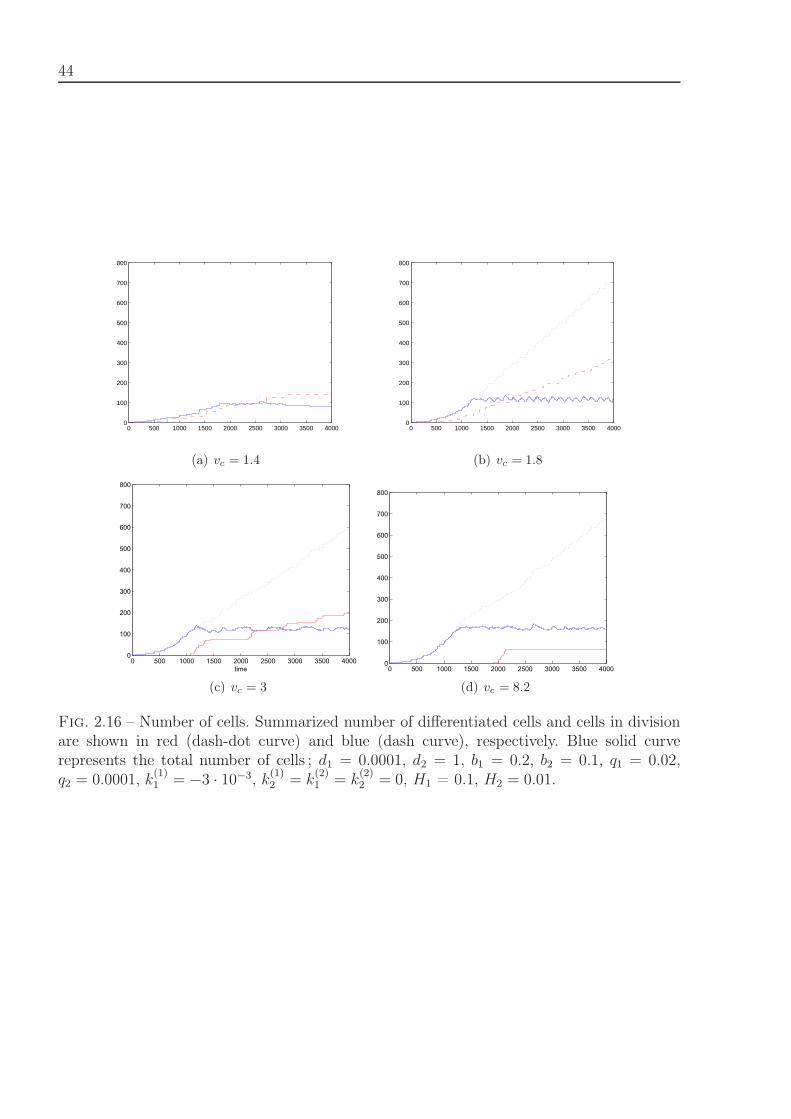
44

0 500 1000 1500 2000 2500 3000 3500 40000

100

200

300

400

500

600

700

800

(a) vc = 1.4

0 500 1000 1500 2000 2500 3000 3500 40000

100

200

300

400

500

600

700

800

(b) vc = 1.8

0 500 1000 1500 2000 2500 3000 3500 40000

100

200

300

400

500

600

700

800

time

(c) vc = 3

0 500 1000 1500 2000 2500 3000 3500 40000

100

200

300

400

500

600

700

800

(d) vc = 8.2

Fig. 2.16 – Number of cells. Summarized number of differentiated cells and cells in divisionare shown in red (dash-dot curve) and blue (dash curve), respectively. Blue solid curverepresents the total number of cells ; d1 = 0.0001, d2 = 1, b1 = 0.2, b2 = 0.1, q1 = 0.02,q2 = 0.0001, k

(1)1 = −3 · 10−3, k

(1)2 = k

(2)1 = k

(2)2 = 0, H1 = 0.1, H2 = 0.01.

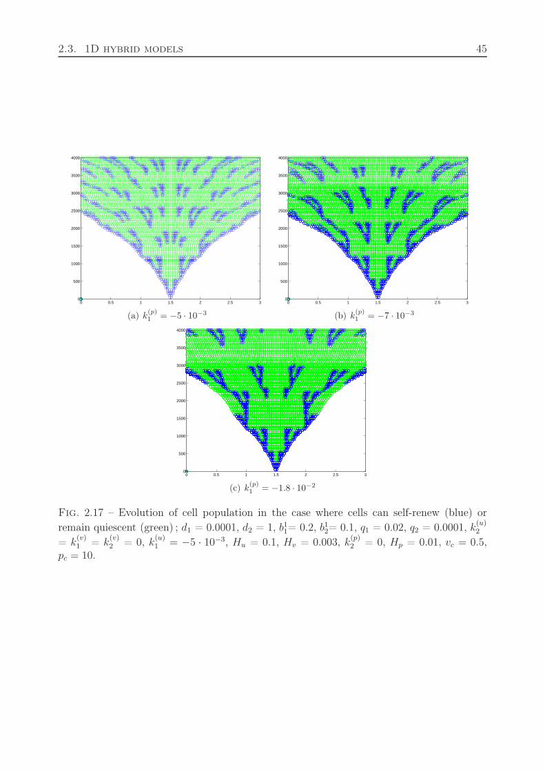
2.3. 1D hybrid models 45

0 0.5 1 1.5 2 2.5 30

500

1000

1500

2000

2500

3000

3500

4000

(a) k(p)1 = −5 · 10−3

0 0.5 1 1.5 2 2.5 30

500

1000

1500

2000

2500

3000

3500

4000

(b) k(p)1 = −7 · 10−3

0 0.5 1 1.5 2 2.5 30

500

1000

1500

2000

2500

3000

3500

4000

(c) k(p)1 = −1.8 · 10−2

Fig. 2.17 – Evolution of cell population in the case where cells can self-renew (blue) or

remain quiescent (green) ; d1 = 0.0001, d2 = 1, b11= 0.2, b1

2= 0.1, q1 = 0.02, q2 = 0.0001, k(u)2

= k(v)1 = k

(v)2 = 0, k

(u)1 = −5 · 10−3, Hu = 0.1, Hv = 0.003, k

(p)2 = 0, Hp = 0.01, vc = 0.5,

pc = 10.

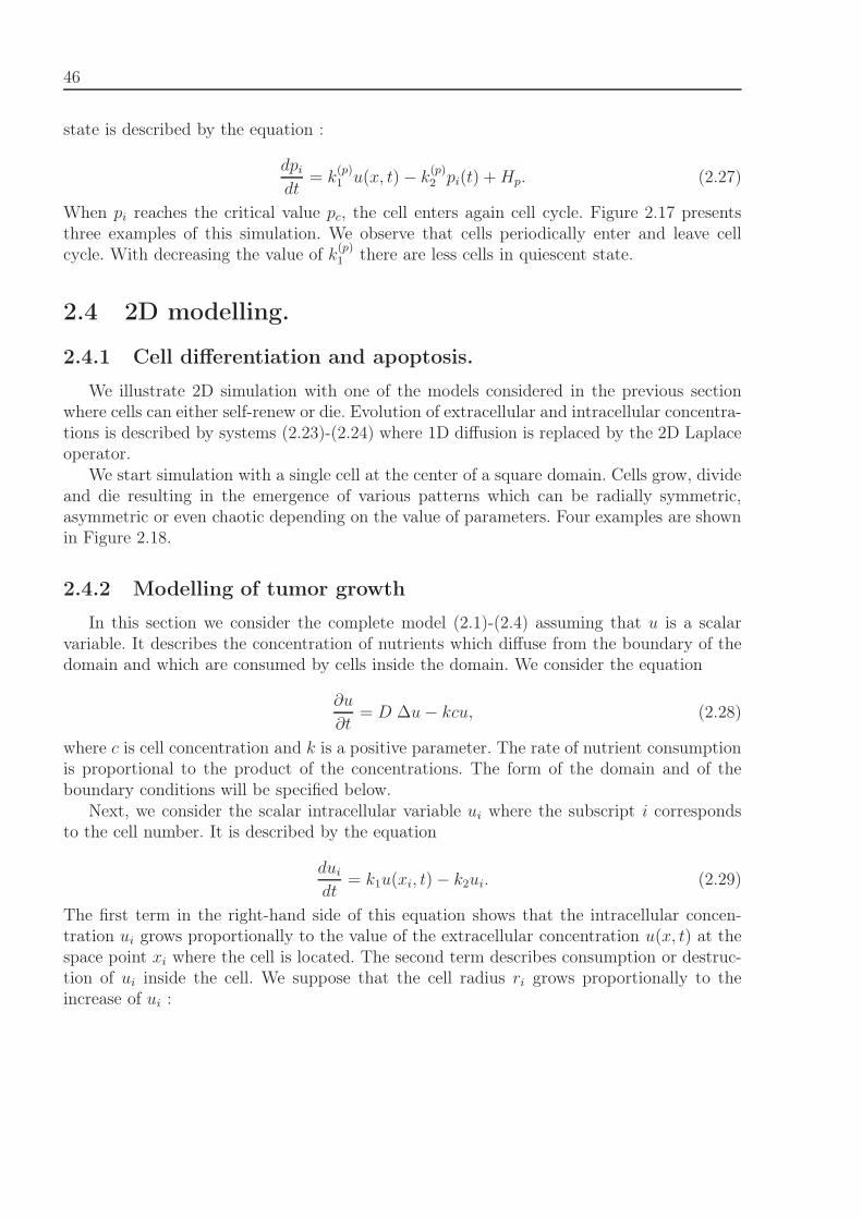
46

state is described by the equation :

dpi

dt= k

(p)1 u(x, t) − k

(p)2 pi(t) + Hp. (2.27)

When pi reaches the critical value pc, the cell enters again cell cycle. Figure 2.17 presentsthree examples of this simulation. We observe that cells periodically enter and leave cellcycle. With decreasing the value of k

(p)1 there are less cells in quiescent state.

2.4 2D modelling.

2.4.1 Cell differentiation and apoptosis.

We illustrate 2D simulation with one of the models considered in the previous sectionwhere cells can either self-renew or die. Evolution of extracellular and intracellular concentra-tions is described by systems (2.23)-(2.24) where 1D diffusion is replaced by the 2D Laplaceoperator.

We start simulation with a single cell at the center of a square domain. Cells grow, divideand die resulting in the emergence of various patterns which can be radially symmetric,asymmetric or even chaotic depending on the value of parameters. Four examples are shownin Figure 2.18.

2.4.2 Modelling of tumor growth

In this section we consider the complete model (2.1)-(2.4) assuming that u is a scalarvariable. It describes the concentration of nutrients which diffuse from the boundary of thedomain and which are consumed by cells inside the domain. We consider the equation

∂u

∂t= D Δu − kcu, (2.28)

where c is cell concentration and k is a positive parameter. The rate of nutrient consumptionis proportional to the product of the concentrations. The form of the domain and of theboundary conditions will be specified below.

Next, we consider the scalar intracellular variable ui where the subscript i correspondsto the cell number. It is described by the equation

dui

dt= k1u(xi, t) − k2ui. (2.29)

The first term in the right-hand side of this equation shows that the intracellular concen-tration ui grows proportionally to the value of the extracellular concentration u(x, t) at thespace point xi where the cell is located. The second term describes consumption or destruc-tion of ui inside the cell. We suppose that the cell radius ri grows proportionally to theincrease of ui :

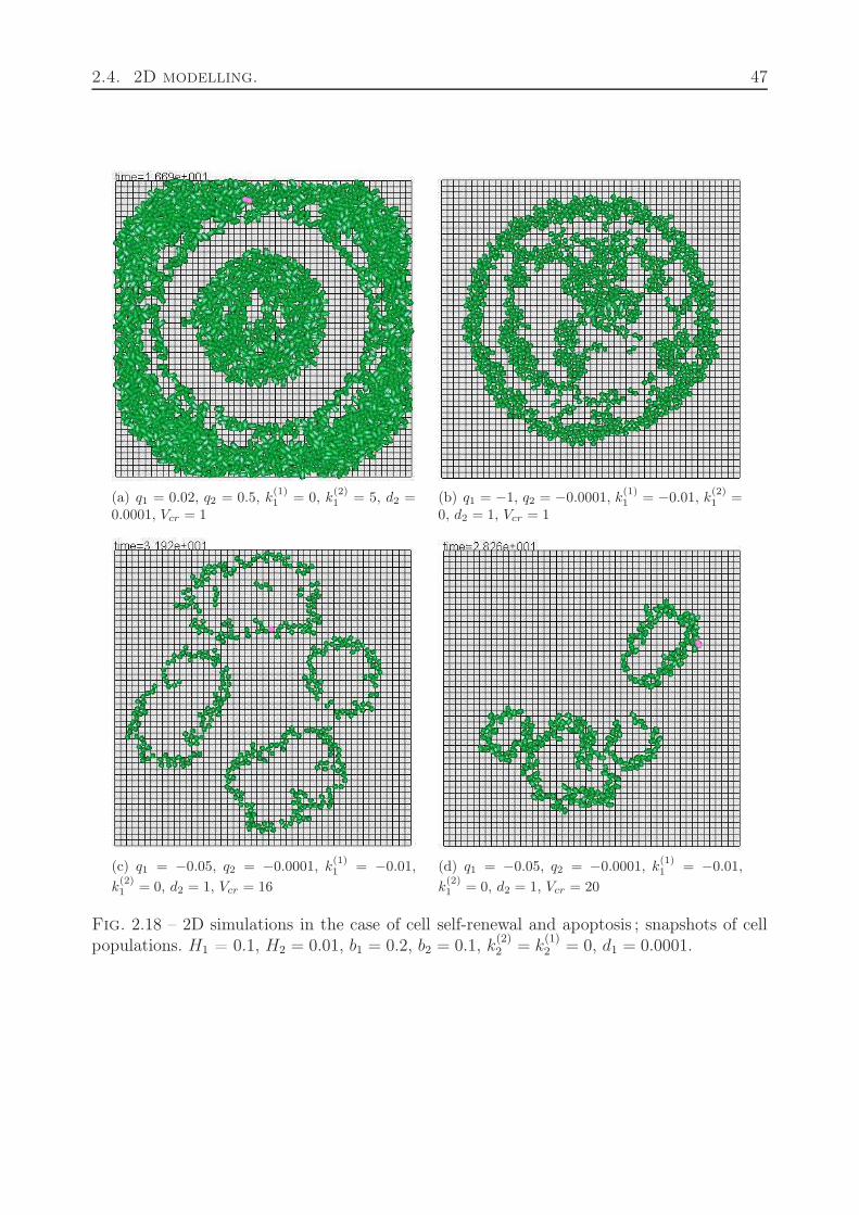
2.4. 2D modelling. 47

(a) q1 = 0.02, q2 = 0.5, k(1)1 = 0, k

(2)1 = 5, d2 =

0.0001, Vcr = 1(b) q1 = −1, q2 = −0.0001, k

(1)1 = −0.01, k

(2)1 =

0, d2 = 1, Vcr = 1

(c) q1 = −0.05, q2 = −0.0001, k(1)1 = −0.01,

k(2)1 = 0, d2 = 1, Vcr = 16

(d) q1 = −0.05, q2 = −0.0001, k(1)1 = −0.01,

k(2)1 = 0, d2 = 1, Vcr = 20

Fig. 2.18 – 2D simulations in the case of cell self-renewal and apoptosis ; snapshots of cellpopulations. H1 = 0.1, H2 = 0.01, b1 = 0.2, b2 = 0.1, k

(2)2 = k

(1)2 = 0, d1 = 0.0001.

48

Fig. 2.19 – Consecutive moments of tumor growth. It starts with a single cell at the centerof the circle. Living cells are shown in red, dead cells in black. 2D grey surface shows thelevel of nutrients.

dri

dt= max

(dui

dt, 0

). (2.30)

The initial value of the radius for each new cell is r0, the maximal radius rm. When it isreached, the cell divides. If the cell does not divide before its maximal age, then it dies. Themaximal cell age is a parameter of the problem.

Consider a circular domain Ω and complete equation (2.28) by the boundary conditionu = 1 at the boundary ∂Ω. We put a single cell in the center of the domain and begin nume-rical solution of system (2.28)-(2.30). The results of the simulations are shown in Figure 2.19for several consecutive moments of time. The grey 2D surface shows the spatial distributionof the concentration u(x, t). In the beginning it equals 1 everywhere in the domain. Theconstants k1 and k2, k1 > k2 are chosen in such a way that the intracellular concentration ui

growth. Consequently, the radius of the cell also grows and after some time the cell divides.The new cells also consume nutrients, grow and divide. The part of the domain filled by cellsforms a disk while the concentration u(x, t) decreases in the center of the domain (secondfigure in the upper row). Hence, the right-hand side of equation (2.30) also decreases, theintracellular concentration stops growing or even decreases, and cells cannot divide beforetheir maximal age τ . As a result, they die and form the black region in the center. Livingcells shown in red form a narrow external layer. The region filled by cells grows in time andfinally approaches to the boundary of the domain.

Dynamics of the cell population can be more complex if we decrease the maximal lifetime τ . Cells now have less time to accumulate enough nutrients for division. In this case,even a small decrease in nutrient concentration can become crucial from the point of view

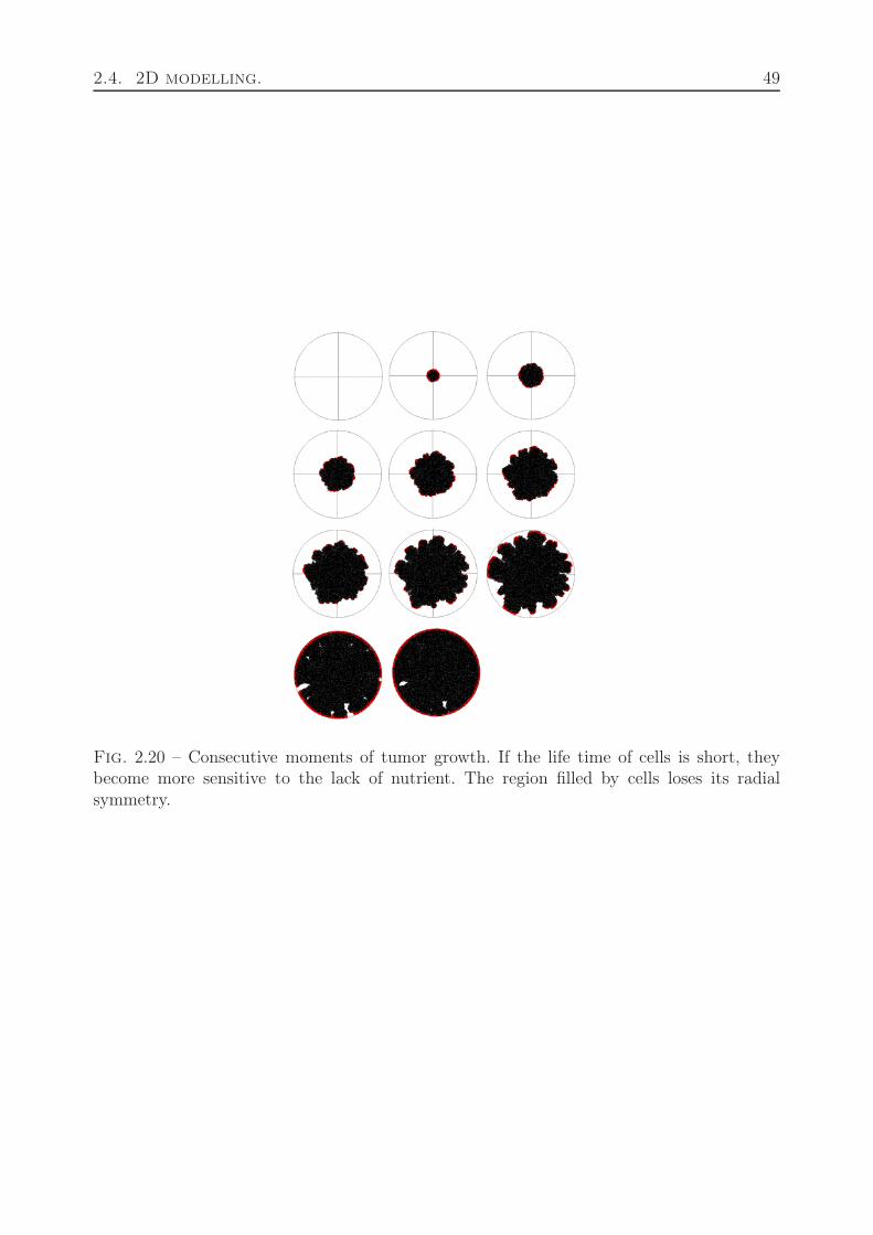
2.4. 2D modelling. 49

Fig. 2.20 – Consecutive moments of tumor growth. If the life time of cells is short, theybecome more sensitive to the lack of nutrient. The region filled by cells loses its radialsymmetry.

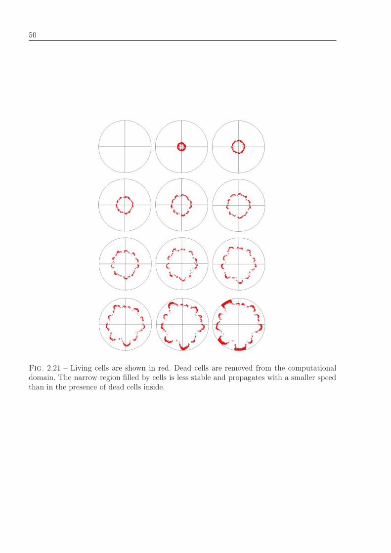
50

Fig. 2.21 – Living cells are shown in red. Dead cells are removed from the computationaldomain. The narrow region filled by cells is less stable and propagates with a smaller speedthan in the presence of dead cells inside.

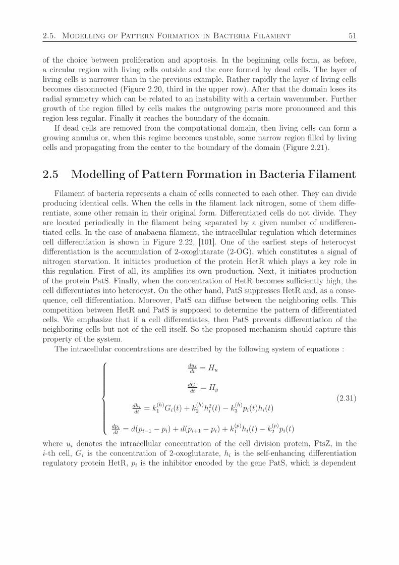
2.5. Modelling of Pattern Formation in Bacteria Filament 51

of the choice between proliferation and apoptosis. In the beginning cells form, as before,a circular region with living cells outside and the core formed by dead cells. The layer ofliving cells is narrower than in the previous example. Rather rapidly the layer of living cellsbecomes disconnected (Figure 2.20, third in the upper row). After that the domain loses itsradial symmetry which can be related to an instability with a certain wavenumber. Furthergrowth of the region filled by cells makes the outgrowing parts more pronounced and thisregion less regular. Finally it reaches the boundary of the domain.

If dead cells are removed from the computational domain, then living cells can form agrowing annulus or, when this regime becomes unstable, some narrow region filled by livingcells and propagating from the center to the boundary of the domain (Figure 2.21).

2.5 Modelling of Pattern Formation in Bacteria Filament

Filament of bacteria represents a chain of cells connected to each other. They can divideproducing identical cells. When the cells in the filament lack nitrogen, some of them diffe-rentiate, some other remain in their original form. Differentiated cells do not divide. Theyare located periodically in the filament being separated by a given number of undifferen-tiated cells. In the case of anabaena filament, the intracellular regulation which determinescell differentiation is shown in Figure 2.22, [101]. One of the earliest steps of heterocystdifferentiation is the accumulation of 2-oxoglutarate (2-OG), which constitutes a signal ofnitrogen starvation. It initiates production of the protein HetR which plays a key role inthis regulation. First of all, its amplifies its own production. Next, it initiates productionof the protein PatS. Finally, when the concentration of HetR becomes sufficiently high, thecell differentiates into heterocyst. On the other hand, PatS suppresses HetR and, as a conse-quence, cell differentiation. Moreover, PatS can diffuse between the neighboring cells. Thiscompetition between HetR and PatS is supposed to determine the pattern of differentiatedcells. We emphasize that if a cell differentiates, then PatS prevents differentiation of theneighboring cells but not of the cell itself. So the proposed mechanism should capture thisproperty of the system.

The intracellular concentrations are described by the following system of equations :⎧⎪⎪⎪⎪⎪⎪⎪⎪⎪⎨⎪⎪⎪⎪⎪⎪⎪⎪⎪⎩

dui

dt= Hu

dGi

dt= Hg

dhi

dt= k

(h)1 Gi(t) + k

(h)2 h2

i (t) − k(h)3 pi(t)hi(t)

dpi

dt= d(pi−1 − pi) + d(pi+1 − pi) + k

(p)1 hi(t) − k

(p)2 pi(t)

(2.31)

where ui denotes the intracellular concentration of the cell division protein, FtsZ, in thei-th cell, Gi is the concentration of 2-oxoglutarate, hi is the self-enhancing differentiationregulatory protein HetR, pi is the inhibitor encoded by the gene PatS, which is dependent

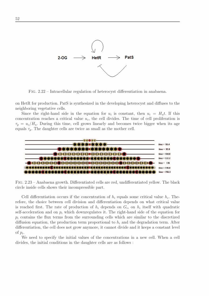
52

Fig. 2.22 – Intracellular regulation of heterocyst differentiation in anabaena.

on HetR for production. PatS is synthesized in the developing heterocyst and diffuses to theneighboring vegetative cells.

Since the right-hand side in the equation for ui is constant, then ui = Hut. If thisconcentration reaches a critical value uc, the cell divides. The time of cell proliferation isτp = uc/Hu. During this time, cell grows linearly and becomes twice bigger when its ageequals τp. The daughter cells are twice as small as the mother cell.

Fig. 2.23 – Anabaena growth. Differentiated cells are red, undifferentiated yellow. The blackcircle inside cells shows their incompressible part.

Cell differentiation occurs if the concentration of hi equals some critical value hc. The-refore, the choice between cell division and differentiation depends on what critical valueis reached first. The rate of production of hi depends on Gi, on hi itself with quadraticself-acceleration and on pi which downregulates it. The right-hand side of the equation forpi contains the flux terms from the surrounding cells which are similar to the discretizeddiffusion equation, the production term proportional to hi and the degradation term. Afterdifferentiation, the cell does not grow anymore, it cannot divide and it keeps a constant levelof pi.

We need to specify the initial values of the concentrations in a new cell. When a celldivides, the initial conditions in the daughter cells are as follows :

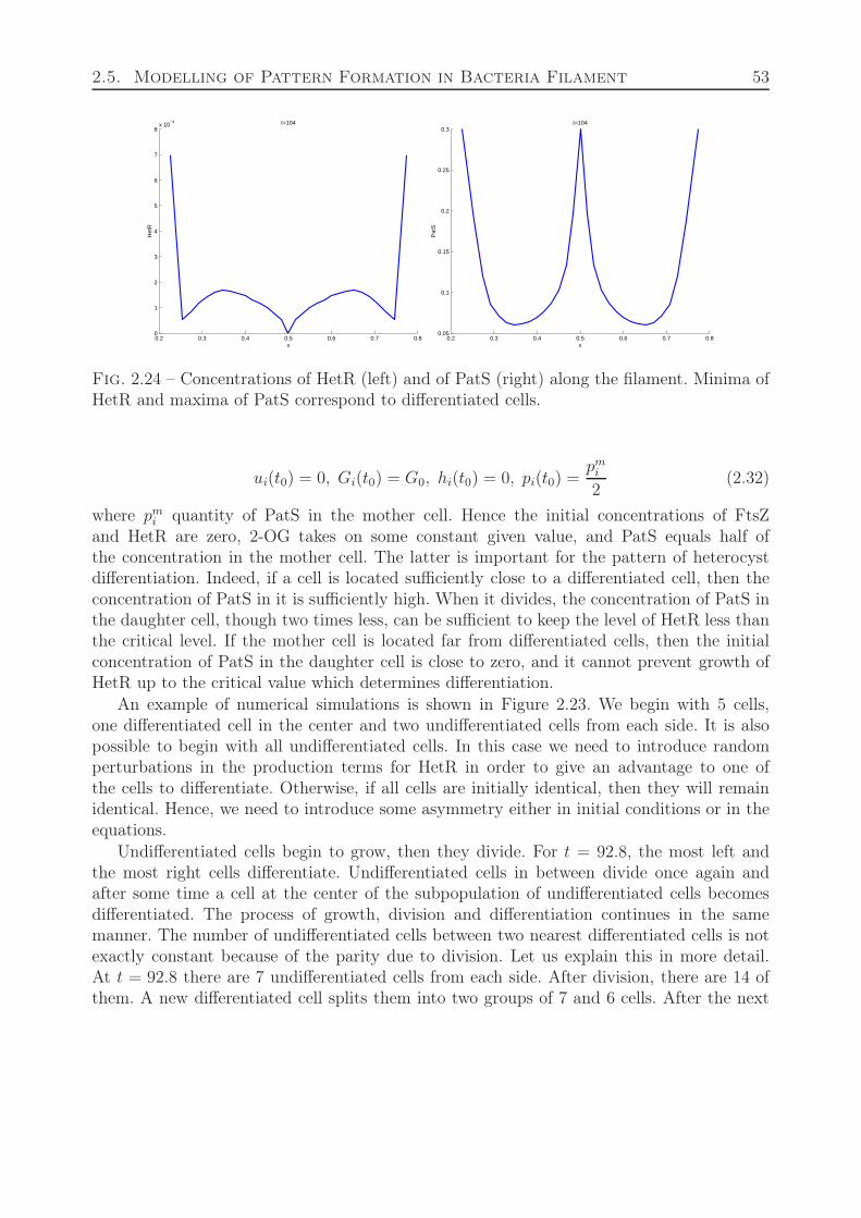
2.5. Modelling of Pattern Formation in Bacteria Filament 53

0.2 0.3 0.4 0.5 0.6 0.7 0.80

1

2

3

4

5

6

7

8x 10

−3

x

Het

R

t=104

0.2 0.3 0.4 0.5 0.6 0.7 0.80.05

0.1

0.15

0.2

0.25

0.3

x

Pat

S

t=104

Fig. 2.24 – Concentrations of HetR (left) and of PatS (right) along the filament. Minima ofHetR and maxima of PatS correspond to differentiated cells.

ui(t0) = 0, Gi(t0) = G0, hi(t0) = 0, pi(t0) =pm

i

2(2.32)

where pmi quantity of PatS in the mother cell. Hence the initial concentrations of FtsZ

and HetR are zero, 2-OG takes on some constant given value, and PatS equals half ofthe concentration in the mother cell. The latter is important for the pattern of heterocystdifferentiation. Indeed, if a cell is located sufficiently close to a differentiated cell, then theconcentration of PatS in it is sufficiently high. When it divides, the concentration of PatS inthe daughter cell, though two times less, can be sufficient to keep the level of HetR less thanthe critical level. If the mother cell is located far from differentiated cells, then the initialconcentration of PatS in the daughter cell is close to zero, and it cannot prevent growth ofHetR up to the critical value which determines differentiation.

An example of numerical simulations is shown in Figure 2.23. We begin with 5 cells,one differentiated cell in the center and two undifferentiated cells from each side. It is alsopossible to begin with all undifferentiated cells. In this case we need to introduce randomperturbations in the production terms for HetR in order to give an advantage to one ofthe cells to differentiate. Otherwise, if all cells are initially identical, then they will remainidentical. Hence, we need to introduce some asymmetry either in initial conditions or in theequations.

Undifferentiated cells begin to grow, then they divide. For t = 92.8, the most left andthe most right cells differentiate. Undifferentiated cells in between divide once again andafter some time a cell at the center of the subpopulation of undifferentiated cells becomesdifferentiated. The process of growth, division and differentiation continues in the samemanner. The number of undifferentiated cells between two nearest differentiated cells is notexactly constant because of the parity due to division. Let us explain this in more detail.At t = 92.8 there are 7 undifferentiated cells from each side. After division, there are 14 ofthem. A new differentiated cell splits them into two groups of 7 and 6 cells. After the next

54

division, there are 14 and 12 cells. The next differentiation will produce the groups of 7, 6,6, and 5 cells. Hence, after each cycle, there is a group of undifferentiated cells smaller thanpreviously. At some point, there will be a group small enough such that it will not give adifferentiated cell. Then the cells in this group will divide producing a group of cells twicelarger.

Figure 2.24 shows the concentrations of HetR and PatS along the filament at t = 104.8 (cf.Figure 2.23). The minima of HetR and the maxima of PatS correspond to the differentiatedcells. Cells differentiate if the value of HetR is sufficiently high. The values of HetR at theboundary cells is still high because these cells have just differentiated.

55

Chapitre 3

Hybrid modeling of erythropoiesis

In this part of the work we use a hybrid model to take into account both intracellular andextracellular regulation of erythropoiesis, but also mainly to study the importance of spatialstructure of erythroblastic islands in the regulation of erythropoiesis. To our knowledge, thisis the first attempt to model erythropoiesis by taking these aspects into account. We focus inparticular on the role of the macrophage, by analyzing different situations, with and withoutmacrophage at the center of the island, and actions of the feedback controls, especiallyregarding the feedback of the macrophage on erythroid cell proliferation and differentiation.The ‘classical’ structure of the erythroblastic island, with the macrophage at the center andimmature erythroid cells surrounding it, will be shown to make the hybrid model stable (sothe island can be sustained for an unlimited number of cell cycles) and robust to perturbationsdue to global and local feedback controls. Following the perturbation, such as an inducedanemia, the return to a healthy organism as soon as in experimental data in mice is observed.The hybrid model displays interesting properties to reproduce erythropoiesis in normal andstress situations, considering spatial aspects of this process.

To present multiscale hybrid model, first, we focus on the intracellular scale, detailingregulatory networks considered in this thesis, described by nonlinear ordinary differentialequations, and investigating their properties, in particular regarding the existence and sta-bility of steady states associated to cell self-renewal, differentiation and death by apoptosis.Second, we concentrate on the extracellular scale, which consists in erythroid cell popula-tions, possibly a macrophage, bone marrow medium, and is described by a computationalmodel. Interactions between cells and with the surrounding medium are presented. Finally,we justify the coupling of both scales, through global and local feedback controls, and wediscuss parameters of the model. In Section 3.2 we present the analysis of the hybrid model.This analysis consists of two parts : first, we consider an erythroblastic island without amacrophage in its center, and investigate the stability of the island and the roles of feed-back controls in the stability. Next we study an island consisting of immature erythroid cellssurrounding a macrophage, and the roles of feedback controls in its stability. This analysisconcludes to the central role of the macrophage in the stability of the erythroblastic island,and consequently of the relevance of considering spatial aspects when modeling erythropoie-

56

sis. Finally, we confront the results of modelling with experiments on anemia in mice.

3.1 Model

We introduce, in this section, the hybrid model for erythropoiesis used later for in silicoexperiments. It consists in the coupling of two models, with different space and time scales.The first model describes intracellular dynamics, represented by regulatory networks basedon specific protein competition. This intracellular dynamical level can be easily modeledwith a continuous approach, namely ordinary differential equations (ODEs) and/or partialdifferential equations (PDEs). The second model is at cell population level, where discretecells and events are computed, so that stochasticity due to random events (cell cycle duration,orientation of the mitotic spindle at division) and small population effects plays an importantrole. Extracellular regulation by growth factors is partially due to continuous models (PDEs).Such discrete-continuous models are usually called hybrid models [19, 51, 83, 88, 90, 102, 111].We hereafter present how the model is defined at each scale and how the different levelsinteract.

3.1.1 Intracellular Scale : Mathematical Model

The intracellular scale describes how each erythroid progenitor cell chooses between self-renewal, differentiation and apoptosis. This choice depends on the level of expression of someproteins, involved in a regulatory network.

Ordinary differential equations are used to describe a simplified regulatory network, basedon two competing proteins, Erk and Fas. Concentrations of the proteins evolve according toprotein-related mechanisms as well as extracellular factor concentrations. A brief analysis ofthe dynamics of the system (3.1)–(3.2) is performed in order to identify key factors in cellfate choice.

3.1.1.1 ODE System

Precise intracellular regulatory mechanisms involved in erythroid progenitor cell fateare largely unknown. Based on the current knowledge, we decided to focus on a simplifiedregulatory network based on two proteins, Erk and Fas, responsible respectively for cellself-renewal and proliferation and cell differentiation and apoptosis [28, 37, 79, 99]. Theseproteins are antagonists : they inhibit each other’s expression. They are also subject toexternal regulation, through feedback loops.

One of these feedback loops is based upon the population of reticulocytes (differentiatederythroid cells). They produce Fas-ligand which is fixed to their exterior cell membrane.Fas-ligand activates Fas, a transmembrane protein, and influences progenitor differentiationand apoptosis. Another feedback control is related to erythrocytes in bloodstream. Theirquantity determines the release of erythropoietin and other hormones, called growth fac-tors. Erythropoietin is known to inhibit erythroid progenitor apoptosis [60] and to stimulate

3.1. Model 57

immature erythroid progenitor self-renewal [99, 112]. Other hormones, like glucocorticoids[14, 45, 46, 84], also increase erythroid progenitor self-renewal by activating Erk.

The simplified system of Erk-Fas interactions considered as the main regulatory networkfor erythroid progenitor fate is then [29]

dEi

dt= (α(Epo, GF ) + βEk

i )(1 − Ei) − aEi − bEiFi, (3.1)

dFi

dt= γ(FL)(1 − Fi) − cEiFi − dFi, (3.2)

where Ei and Fi denote intracellular normalized levels of Erk and Fas, respectively, in thei-th cell (numbering of cells is related to the discrete off-lattice model). Intracellular concen-tration Ei and Fi are supposed to be uniform inside the i-th cell. They depend on timeand independent of space. Their values can be different in different cells. Equation (3.1)describes how Erk level evolves toward maximal value 1 by activation through hormones(function α of erythropoeitin, denoted by Epo, and other growth factors, denoted by GF )and self-activation (parameters β and k). In the meantime, Erk is linearly degraded with arate a and is inhibited by Fas with a rate bF . Erythropoietin concentration depends only ontime.

Equation (3.2) is very similar, only there is no proof for Fas self-activation. Fas is howeveractivitated by Fas-ligand extracellular concentration, denoted by FL, through the functionγ(FL), it is degraded with a rate d and inhibited by Erk with a rate cE. Fas-ligand concen-tration depends on time and space.

This model simply describes a competition between two proteins (Erk and Fas) throughcross-inhibition, self-activation (only for Erk), and activation by extracellular proteins.

In order to explore the parameter space efficiently and observe the possible behaviors ofthe cell, it is relevant to study the mathematical interpretation of parameters.

3.1.1.2 Brief Analysis : Existence and Stability of Steady States

For fixed values of Epo, GF and FL, (3.1)-(3.2) is a closed system of ordinary differentialequations. In order to analyze the impact of each parameter on the system’s behavior, wecan derive analytical forms of the zero-lines associated with each equation. The zero-line fassociated with equation (3.1) is

f(E) =1

b

( α

E− βEk−1(1 − E) − (a + α)

). (3.3)

The zero-line g associated with equation (3.2) is

g(E) =

γ

cγ + d

c+ E

. (3.4)

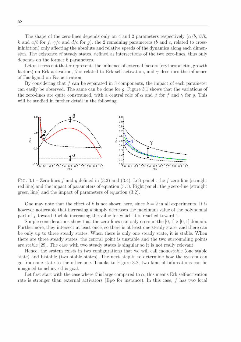
58

The shape of the zero-lines depends only on 4 and 2 parameters respectively (α/b, β/b,k and a/b for f , γ/c and d/c for g), the 2 remaining parameters (b and c, related to cross-inhibition) only affecting the absolute and relative speeds of the dynamics along each dimen-sion. The existence of steady states, defined as intersections of the two zero-lines, thus onlydepends on the former 6 parameters.

Let us stress out that α represents the influence of external factors (erythropoietin, growthfactors) on Erk activation, β is related to Erk self-activation, and γ describes the influenceof Fas-ligand on Fas activation.

By considering that f can be separated in 3 components, the impact of each parametercan easily be observed. The same can be done for g. Figure 3.1 shows that the variations ofthe zero-lines are quite constrained, with a central role of α and β for f and γ for g. Thiswill be studied in further detail in the following.

β

α

a

d γ

Fig. 3.1 – Zero-lines f and g defined in (3.3) and (3.4). Left panel : the f zero-line (straightred line) and the impact of parameters of equation (3.1). Right panel : the g zero-line (straightgreen line) and the impact of parameters of equation (3.2).

One may note that the effect of k is not shown here, since k = 2 in all experiments. It ishowever noticeable that increasing k simply decreases the maximum value of the polynomialpart of f toward 0 while increasing the value for which it is reached toward 1.

Simple considerations show that the zero-lines can only cross in the [0, 1]× [0, 1] domain.Furthermore, they intersect at least once, so there is at least one steady state, and there canbe only up to three steady states. When there is only one steady state, it is stable. Whenthere are three steady states, the central point is unstable and the two surrounding pointsare stable [29]. The case with two steady states is singular so it is not really relevant.

Hence, the system exists in two configurations that we will call monostable (one stablestate) and bistable (two stable states). The next step is to determine how the system cango from one state to the other one. Thanks to Figure 3.2, two kind of bifurcations can beimagined to achieve this goal.

Let first start with the case where β is large compared to α, this means Erk self-activationrate is stronger than external activators (Epo for instance). In this case, f has two local

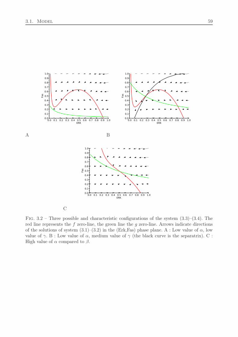
3.1. Model 59

A B

C

Fig. 3.2 – Three possible and characteristic configurations of the system (3.3)–(3.4). Thered line represents the f zero-line, the green line the g zero-line. Arrows indicate directionsof the solutions of system (3.1)–(3.2) in the (Erk,Fas) phase plane. A : Low value of α, lowvalue of γ. B : Low value of α, medium value of γ (the black curve is the separatrix). C :High value of α compared to β.

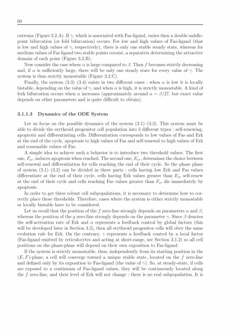
60

extrema (Figure 3.2.A). If γ, which is associated with Fas-ligand, varies then a double saddle-point bifurcation (or fold bifurcation) occurs. For low and high values of Fas-ligand (thatis low and high values of γ, respectively), there is only one stable steady state, whereas formedium values of Fas ligand two stable points coexist, a separatrix determining the attractivedomain of each point (Figure 3.2.B).

Now consider the case where α is large compared to β. Then f becomes strictly decreasingand, if α is sufficiently large, there will be only one steady state for every value of γ. Thesystem is thus strictly monostable (Figure 3.2.C).

Finally, the system (3.3)–(3.4) exists in two different cases : when α is low it is locallybistable, depending on the value of γ, and when α is high, it is strictly monostable. A kind offork bifurcation occurs when α increases (approximately around α = β/27, but exact valuedepends on other parameters and is quite difficult to obtain).

3.1.1.3 Dynamics of the ODE System

Let us focus on the possible dynamics of the system (3.1)–(3.2). This system must beable to divide the erythroid progenitor cell population into 3 different types : self-renewing,apoptotic and differentiating cells. Differentiation corresponds to low values of Fas and Erkat the end of the cycle, apoptosis to high values of Fas and self-renewal to high values of Erkand reasonable values of Fas.

A simple idea to achieve such a behavior is to introduce two threshold values. The firstone, Fcr, induces apoptosis when reached. The second one, Ecr, determines the choice betweenself-renewal and differentiation for cells reaching the end of their cycle. So the phase planeof system (3.1)–(3.2) can be divided in three parts : cells having low Erk and Fas valuesdifferentiate at the end of their cycle, cells having Erk values greater than Ecr self-renewat the end of their cycle and cells reaching Fas values greater than Fcr die immediately byapoptosis.

In order to get three robust cell subpopulations, it is necessary to determine how to cor-rectly place these thresholds. Therefore, cases where the system is either strictly monostableor locally bistable have to be considered.

Let us recall that the position of the f zero-line strongly depends on parameters α and β,whereas the position of the g zero-line strongly depends on the parameter γ. Since β denotesthe self-activation rate of Erk and α represents a feedback control by global factors (thiswill be developed later in Section 3.2), then all erythroid progenitor cells will obey the sameevolution rule for Erk. On the contrary, γ represents a feedback control by a local factor(Fas-ligand emitted by reticulocytes and acting at short-range, see Section 3.1.2) so all cellpositions on the phase-plane will depend on their own exposition to Fas-ligand.

If the system is strictly monostable, then, independently from its starting position in the(E, F )-plane, a cell will converge toward a unique stable state, located on the f zero-lineand defined only by its exposition to Fas-ligand (the value of γ). So, at steady-state, if cellsare exposed to a continuum of Fas-ligand values, they will be continuously located alongthe f zero-line, and their level of Erk will not change : there is no real subpopulation. It is

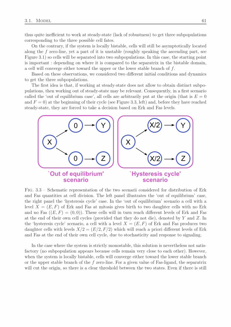
3.1. Model 61

thus quite inefficient to work at steady-state (lack of robustness) to get three subpopulationscorresponding to the three possible cell fates.

On the contrary, if the system is locally bistable, cells will still be asymptotically locatedalong the f zero-line, yet a part of it is unstable (roughly speaking the ascending part, seeFigure 3.1) so cells will be separated into two subpopulations. In this case, the starting pointis important : depending on where it is compared to the separatrix in the bistable domain,a cell will converge either toward the upper or the lower stable branch of f .

Based on these observations, we considered two different initial conditions and dynamicsto get the three subpopulations.

The first idea is that, if working at steady-state does not allow to obtain distinct subpo-pulations, then working out of steady-state may be relevant. Consequently, in a first scenariocalled the ‘out of equilibrium case’, all cells are arbitrarily put at the origin (that is E = 0and F = 0) at the beginning of their cycle (see Figure 3.3, left) and, before they have reachedsteady-state, they are forced to take a decision based on Erk and Fas levels.

`Out of equilibrium' scenario

`Hysteresis cycle' scenario

X

0

0

X

X/2

X/2

Y

Z Z

Y

Fig. 3.3 – Schematic representation of the two scenarii considered for distribution of Erkand Fas quantities at cell division. The left panel illustrates the ‘out of equilibrium’ case,the right panel the ‘hysteresis cycle’ case. In the ‘out of equilibrium’ scenario a cell with alevel X = (E, F ) of Erk and Fas at mitosis gives birth to two daughter cells with no Erkand no Fas ((E, F ) = (0, 0)). These cells will in turn reach different levels of Erk and Fasat the end of their own cell cycles (provided that they do not die), denoted by Y and Z. Inthe ‘hysteresis cycle’ scenario, a cell with a level X = (E, F ) of Erk and Fas produces twodaughter cells with levels X/2 = (E/2, F/2) which will reach a priori different levels of Erkand Fas at the end of their own cell cycle, due to stochasticity and response to signaling.

In the case where the system is strictly monostable, this solution is nevertheless not satis-factory (no subpopulation appears because cells remain very close to each other). However,when the system is locally bistable, cells will converge either toward the lower stable branchor the upper stable branch of the f zero-line. For a given value of Fas-ligand, the separatrixwill cut the origin, so there is a clear threshold between the two states. Even if there is still

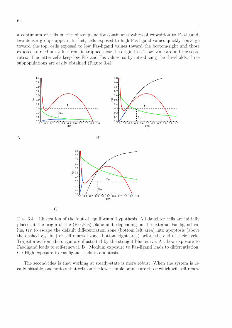
62

a continuum of cells on the phase plane for continuous values of exposition to Fas-ligand,two denser groups appear. In fact, cells exposed to high Fas-ligand values quickly convergetoward the top, cells exposed to low Fas-ligand values toward the bottom-right and thoseexposed to medium values remain trapped near the origin in a ‘slow’ zone around the sepa-ratrix. The latter cells keep low Erk and Fas values, so by introducing the thresholds, threesubpopulations are easily obtained (Figure 3.4).

Ecr

Fcr

Ecr

Fcr

A B

Ecr

Fcr

C

Fig. 3.4 – Illustration of the ‘out of equilibrium’ hypothesis. All daughter cells are initiallyplaced at the origin of the (Erk,Fas) plane and, depending on the external Fas-ligand va-lue, try to escape the default differentiation zone (bottom left area) into apoptosis (abovethe dashed Fcr line) or self-renewal zone (bottom right area) before the end of their cycle.Trajectories from the origin are illustrated by the straight blue curve. A : Low exposure toFas-ligand leads to self-renewal. B : Medium exposure to Fas-ligand leads to differentiation.C : High exposure to Fas-ligand leads to apoptosis.

The second idea is that working at steady-state is more robust. When the system is lo-cally bistable, one notices that cells on the lower stable branch are those which will self-renew

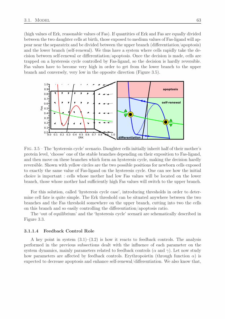
3.1. Model 63

(high values of Erk, reasonable values of Fas). If quantities of Erk and Fas are equally dividedbetween the two daughter cells at birth, those exposed to medium values of Fas-ligand will ap-pear near the separatrix and be divided between the upper branch (differentiation/apoptosis)and the lower branch (self-renewal). We thus have a system where cells rapidly take the de-cision between self-renewal or differentiation/apoptosis. Once the decision is made, cells aretrapped on a hysteresis cycle controlled by Fas-ligand, so the decision is hardly reversible.Fas values have to become very high in order to get from the lower branch to the upperbranch and conversely, very low in the opposite direction (Figure 3.5).

apoptosis

self-renewal

differentiation

Fig. 3.5 – The ‘hysteresis cycle’ scenario. Daughter cells initially inherit half of their mother’sprotein level, ‘choose’ one of the stable branches depending on their exposition to Fas-ligand,and then move on these branches which form an hysteresis cycle, making the decision hardlyreversible. Shown with yellow circles are the two possible positions for newborn cells exposedto exactly the same value of Fas-ligand on the hysteresis cycle. One can see how the initialchoice is important : cells whose mother had low Fas values will be located on the lowerbranch, those whose mother had sufficiently high Fas values will switch to the upper branch.

For this solution, called ‘hysteresis cycle case’, introducing thresholds in order to deter-mine cell fate is quite simple. The Erk threshold can be situated anywhere between the twobranches and the Fas threshold somewhere on the upper branch, cutting into two the cellson this branch and so easily controlling the differentiation/apoptosis ratio.

The ‘out of equilibrium’ and the ‘hysteresis cycle’ scenarii are schematically described inFigure 3.3.

3.1.1.4 Feedback Control Role

A key point in system (3.1)–(3.2) is how it reacts to feedback controls. The analysisperformed in the previous subsections dealt with the influence of each parameter on thesystem dynamics, mainly parameters related to feedback controls (α and γ). Let now studyhow parameters are affected by feedback controls. Erythropoietin (through function α) isexpected to decrease apoptosis and enhance self-renewal/differentiation. We also know that,

64

at a smaller space scale, Fas-ligand induces apoptosis (through function γ) and other growthfactors, on the opposite, stimulate self-renewal (through the function α).

In order to validate possible dynamics, the effect of each factor must be checked in bothcases, the ‘out of equilibrium’ and the ‘hysteresis cycle’ scenarii.

The control exerted by Fas-ligand, which increases the value of Fas reached at steady-state, has already been largely discussed. Simply by existence of the threshold Fcr, Fas-ligandplays the expected role. Fas-ligand is linked to the parameter γ, which is actually a functionof FL.

Epo is known to have a direct action on apoptosis [60], independent of Erk pathway[30, 80, 114]. Therefore, a simple idea is to increase Fcr with the level of Epo. This clearlyreduces apoptosis in favor of differentiation and self-renewal. However, it is also knownthat Epo, and other growth factors, activate Erk. So erythropoietin and growth factors aresupposed to influence the variations of α. It is noticeable that at a local scale, many growthfactors are supposed to have similar mechanisms, so α should in fact be a function of manyglobal and local growth factors.

The value of α controls the monostable/bistable bifurcation (Figure 3.1). When the sys-tem is locally bistable, α mainly controls the value of the local minimum of the f zero-line.In the case where we work out of equilibrium, α changes the position of the separatrix andof the upper steady states, so when α is increased the separatrix cuts the origin for a highervalue of γ(FL) and cells tend to be displaced toward steady-states with lower values of Fasand higher values of Erk. In the case where the hysteresis cycle is used, increasing the localminimum of f reduces the size of the cycle. Cells located on the upper stable branch instantly‘fall’ on the lower stable branch, so self-renewal is immediately enhanced and differentiationreduced.

The effect of α is not the same in both dynamics, but finally it is clearly possible todecrease apoptosis in favor of self-renewal/differentiation and the trends for each protein isroughly what is expected biologically. However, it is still necessary to study whether thefeedback is as efficient as observed experimentally, when the intracellular scale is coupled tothe extracellular one (see Section 3.2).

3.1.2 Extracellular Scale

In the previous section, we focused on the intracellular scale of the hybrid model, based ona system of ordinary differential equations describing competition between two key proteins,Erk and Fas. Concentrations of Erk and Fas induce either cell self-renewal, or differentiation,or death by apoptosis. We now focus on an other layer of the hybrid model, the discrete part,which describes how cells interact and how they influence intracellular parameters whichdepend on extracellular molecules.

In order to describe the evolution of an erythroid cell population, we chose to use anindividual-based model. All cells and their interactions are then numerically computed. Theobjective being to represent erythroblastic islands, which have a limited size, such an ap-proach takes automatically into account small population effects as well as random effects

3.1. Model 65

(direction of division, cell cycle length).A population of cells is numerically simulated in a 2D computational domain which is

a rectangle. Each cell is a discrete object, an elastic ball, considered to be circular andcomposed of two parts : a compressible part at the border and a hardly compressible part atthe center. All newborn cells have the same radius r0 and linearly increase in size until theend of their cycle, when they reach twice the initial radius. When a cell divides, it gives birthto two small cells side by side, the direction of division being randomly chosen. The cell cycleduration is itself variable. From a biological point of view, cell cycle proceeds through G0/G1,S, G2 and M phases. Duration of the first G0/G1 phase and transitions between phases arecontrolled by various intracellular and extracellular mechanisms, inducing stochasticity incell cycle durations [49, 100]. We assumed the duration of G0/G1 phase is a random variablewith a uniform distribution in some given interval, other phase durations were supposed tobe constant.

Under the assumption of small deformations, the force acting between cells can be ex-pressed as a function of the distance between their centers. The force between two particleswith centers at xi and xj is given by a function D(dij) of the distance dij between the centers.This function is zero if the distance is greater than the sum of their radii. To describe themotion of a particle, one should determine the forces acting on it from all other particlesand possibly from the surrounding medium. The motion of each cell is then described by thedisplacement of its center by Newton’s second law :

mx + μmx −∑j �=i

D(dij) = 0, (3.5)

where m is the mass of the particle, the second term in left-hand side describes the frictionby the surrounding medium, the third term is the potential force between cells. The forcebetween two spherical particles is considered in the form

D(dij) =

⎧⎨⎩ K

d0 − dij

dij − d0 + 2H1, dij < d0,

0, dij ≥ d0,

(3.6)

where d0 is the sum of cell radii, K is a positive parameter, and H1 accounts for the compres-sible part of each cell. The force between the particles tends to infinity when dij decreasesto d0 − 2H1. On the other hand, this force equals zero if dij ≥ d0.

Three cell types are computed. First, erythroblasts, which are immature erythroid cells,also known as erythroid progenitors. They follow the growth rules explained above and theirfate is determined as described in Section 3.1.1. They either self-renew and give two cellsof the same type, or differentiate and give two differentiated cells (reticulocytes), or die byapoptosis, depending on their exposition to growth factors and Fas-ligand. It is noticeablethat no asymmetric division is considered in this model.

Second, reticulocytes. From a biological point of view, reticulocytes are almost mature redblood cells that leave the bone marrow and enter the bloodstream after ejecting their nuclei.

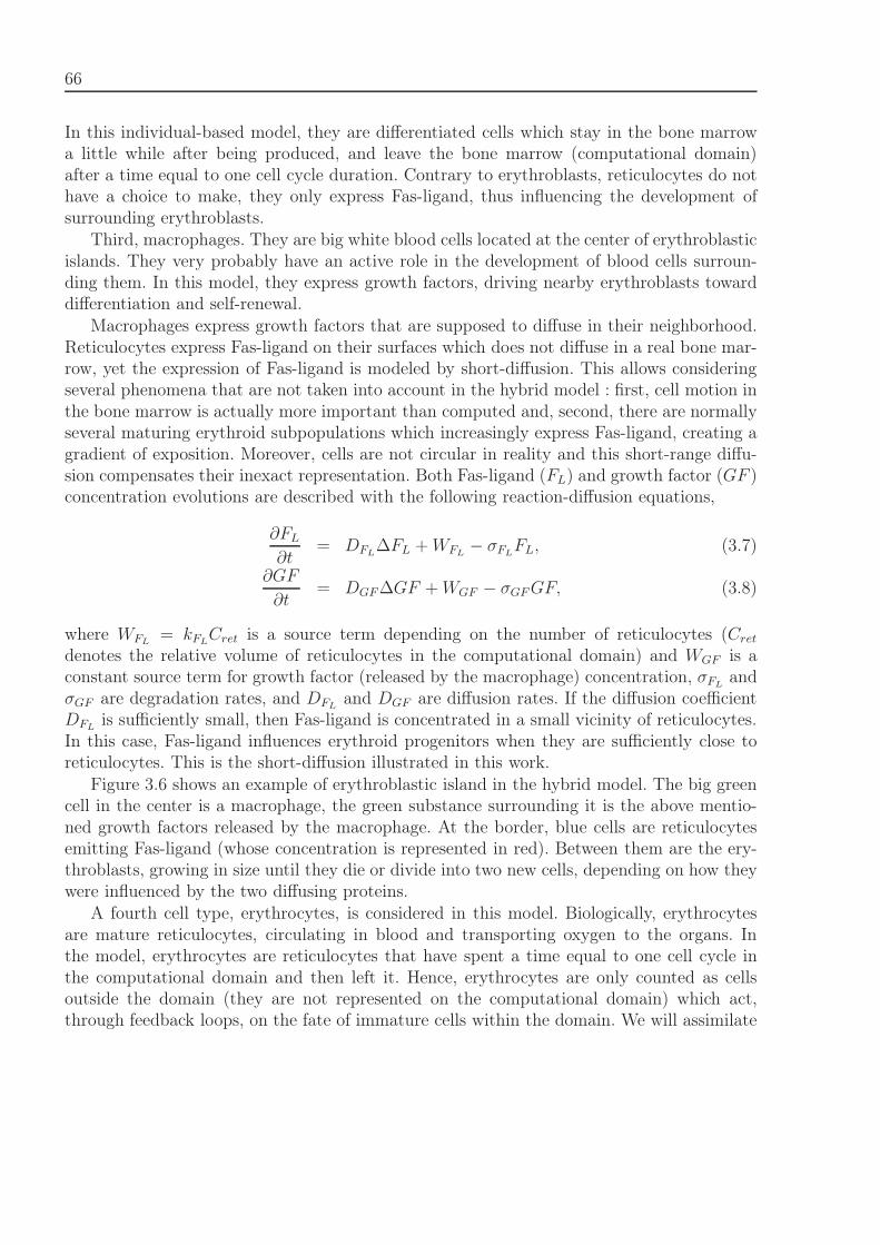
66

In this individual-based model, they are differentiated cells which stay in the bone marrowa little while after being produced, and leave the bone marrow (computational domain)after a time equal to one cell cycle duration. Contrary to erythroblasts, reticulocytes do nothave a choice to make, they only express Fas-ligand, thus influencing the development ofsurrounding erythroblasts.

Third, macrophages. They are big white blood cells located at the center of erythroblasticislands. They very probably have an active role in the development of blood cells surroun-ding them. In this model, they express growth factors, driving nearby erythroblasts towarddifferentiation and self-renewal.

Macrophages express growth factors that are supposed to diffuse in their neighborhood.Reticulocytes express Fas-ligand on their surfaces which does not diffuse in a real bone mar-row, yet the expression of Fas-ligand is modeled by short-diffusion. This allows consideringseveral phenomena that are not taken into account in the hybrid model : first, cell motion inthe bone marrow is actually more important than computed and, second, there are normallyseveral maturing erythroid subpopulations which increasingly express Fas-ligand, creating agradient of exposition. Moreover, cells are not circular in reality and this short-range diffu-sion compensates their inexact representation. Both Fas-ligand (FL) and growth factor (GF )concentration evolutions are described with the following reaction-diffusion equations,

∂FL

∂t= DFL

ΔFL + WFL− σFL

FL, (3.7)

∂GF

∂t= DGFΔGF + WGF − σGF GF, (3.8)

where WFL= kFL

Cret is a source term depending on the number of reticulocytes (Cret

denotes the relative volume of reticulocytes in the computational domain) and WGF is aconstant source term for growth factor (released by the macrophage) concentration, σFL

andσGF are degradation rates, and DFL

and DGF are diffusion rates. If the diffusion coefficientDFL

is sufficiently small, then Fas-ligand is concentrated in a small vicinity of reticulocytes.In this case, Fas-ligand influences erythroid progenitors when they are sufficiently close toreticulocytes. This is the short-diffusion illustrated in this work.

Figure 3.6 shows an example of erythroblastic island in the hybrid model. The big greencell in the center is a macrophage, the green substance surrounding it is the above mentio-ned growth factors released by the macrophage. At the border, blue cells are reticulocytesemitting Fas-ligand (whose concentration is represented in red). Between them are the ery-throblasts, growing in size until they die or divide into two new cells, depending on how theywere influenced by the two diffusing proteins.

A fourth cell type, erythrocytes, is considered in this model. Biologically, erythrocytesare mature reticulocytes, circulating in blood and transporting oxygen to the organs. Inthe model, erythrocytes are reticulocytes that have spent a time equal to one cell cycle inthe computational domain and then left it. Hence, erythrocytes are only counted as cellsoutside the domain (they are not represented on the computational domain) which act,through feedback loops, on the fate of immature cells within the domain. We will assimilate

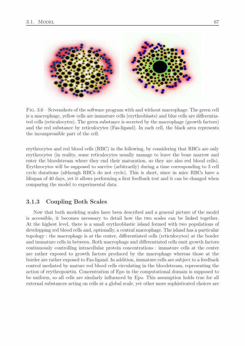
3.1. Model 67

Fig. 3.6 – Screenshots of the software program with and without macrophage. The green cellis a macrophage, yellow cells are immature cells (erythroblasts) and blue cells are differentia-ted cells (reticulocytes). The green substance is secreted by the macrophage (growth factors)and the red substance by reticulocytes (Fas-ligand). In each cell, the black area representsthe incompressible part of the cell.

erythrocytes and red blood cells (RBC) in the following, by considering that RBCs are onlyerythrocytes (in reality, some reticulocytes usually manage to leave the bone marrow andenter the bloodstream where they end their maturation, so they are also red blood cells).Erythrocytes will be supposed to survive (arbitrarily) during a time corresponding to 3 cellcycle durations (although RBCs do not cycle). This is short, since in mice RBCs have alifespan of 40 days, yet it allows performing a first feedback test and it can be changed whencomparing the model to experimental data.

3.1.3 Coupling Both Scales

Now that both modeling scales have been described and a general picture of the modelis accessible, it becomes necessary to detail how the two scales can be linked together.At the highest level, there is a small erythroblastic island formed with two populations ofdevelopping red blood cells and, optionally, a central macrophage. The island has a particulartopology : the macrophage is at the center, differentiated cells (reticulocytes) at the borderand immature cells in between. Both macrophage and differentiated cells emit growth factorscontinuously controlling intracellular protein concentrations : immature cells at the centerare rather exposed to growth factors produced by the macrophage whereas those at theborder are rather exposed to Fas-ligand. In addition, immature cells are subject to a feedbackcontrol mediated by mature red blood cells circulating in the bloodstream, representing theaction of erythropoietin. Concentration of Epo in the computational domain is supposed tobe uniform, so all cells are similarly influenced by Epo. This assumption holds true for allexternal substances acting on cells at a global scale, yet other more sophisticated choices are

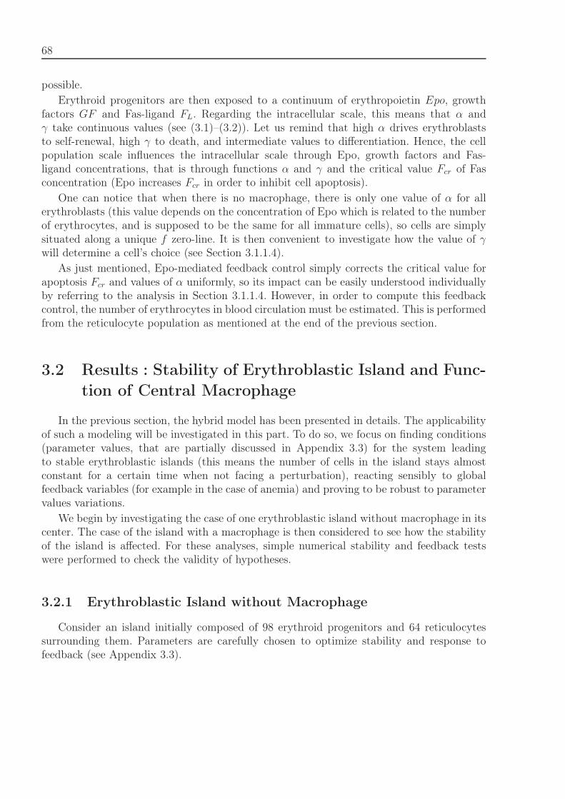
68

possible.

Erythroid progenitors are then exposed to a continuum of erythropoietin Epo, growthfactors GF and Fas-ligand FL. Regarding the intracellular scale, this means that α andγ take continuous values (see (3.1)–(3.2)). Let us remind that high α drives erythroblaststo self-renewal, high γ to death, and intermediate values to differentiation. Hence, the cellpopulation scale influences the intracellular scale through Epo, growth factors and Fas-ligand concentrations, that is through functions α and γ and the critical value Fcr of Fasconcentration (Epo increases Fcr in order to inhibit cell apoptosis).

One can notice that when there is no macrophage, there is only one value of α for allerythroblasts (this value depends on the concentration of Epo which is related to the numberof erythrocytes, and is supposed to be the same for all immature cells), so cells are simplysituated along a unique f zero-line. It is then convenient to investigate how the value of γwill determine a cell’s choice (see Section 3.1.1.4).

As just mentioned, Epo-mediated feedback control simply corrects the critical value forapoptosis Fcr and values of α uniformly, so its impact can be easily understood individuallyby referring to the analysis in Section 3.1.1.4. However, in order to compute this feedbackcontrol, the number of erythrocytes in blood circulation must be estimated. This is performedfrom the reticulocyte population as mentioned at the end of the previous section.

3.2 Results : Stability of Erythroblastic Island and Func-

tion of Central Macrophage

In the previous section, the hybrid model has been presented in details. The applicabilityof such a modeling will be investigated in this part. To do so, we focus on finding conditions(parameter values, that are partially discussed in Appendix 3.3) for the system leadingto stable erythroblastic islands (this means the number of cells in the island stays almostconstant for a certain time when not facing a perturbation), reacting sensibly to globalfeedback variables (for example in the case of anemia) and proving to be robust to parametervalues variations.

We begin by investigating the case of one erythroblastic island without macrophage in itscenter. The case of the island with a macrophage is then considered to see how the stabilityof the island is affected. For these analyses, simple numerical stability and feedback testswere performed to check the validity of hypotheses.

3.2.1 Erythroblastic Island without Macrophage

Consider an island initially composed of 98 erythroid progenitors and 64 reticulocytessurrounding them. Parameters are carefully chosen to optimize stability and response tofeedback (see Appendix 3.3).

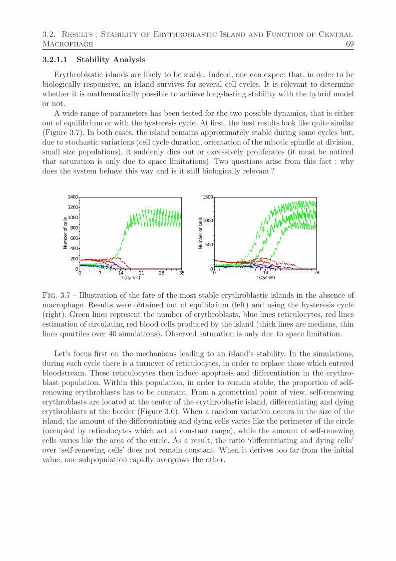
3.2. Results : Stability of Erythroblastic Island and Function of Central

Macrophage 69

3.2.1.1 Stability Analysis

Erythroblastic islands are likely to be stable. Indeed, one can expect that, in order to bebiologically responsive, an island survives for several cell cycles. It is relevant to determinewhether it is mathematically possible to achieve long-lasting stability with the hybrid modelor not.

A wide range of parameters has been tested for the two possible dynamics, that is eitherout of equilibrium or with the hysteresis cycle. At first, the best results look like quite similar(Figure 3.7). In both cases, the island remains approximately stable during some cycles but,due to stochastic variations (cell cycle duration, orientation of the mitotic spindle at division,small size populations), it suddenly dies out or excessively proliferates (it must be noticedthat saturation is only due to space limitations). Two questions arise from this fact : whydoes the system behave this way and is it still biologically relevant ?

0 7 14 21 28 350

200

400

600

800

1000

1200

1400

Num

bero

fcell

s

t (cycles)0 14 28

0

500

1000

1500N

um

be

r o

f ce

lls

t (cycles)

Fig. 3.7 – Illustration of the fate of the most stable erythroblastic islands in the absence ofmacrophage. Results were obtained out of equilibrium (left) and using the hysteresis cycle(right). Green lines represent the number of erythroblasts, blue lines reticulocytes, red linesestimation of circulating red blood cells produced by the island (thick lines are medians, thinlines quartiles over 40 simulations). Observed saturation is only due to space limitation.

Let’s focus first on the mechanisms leading to an island’s stability. In the simulations,during each cycle there is a turnover of reticulocytes, in order to replace those which enteredbloodstream. These reticulocytes then induce apoptosis and differentiation in the erythro-blast population. Within this population, in order to remain stable, the proportion of self-renewing erythroblasts has to be constant. From a geometrical point of view, self-renewingerythroblasts are located at the center of the erythroblastic island, differentiating and dyingerythroblasts at the border (Figure 3.6). When a random variation occurs in the size of theisland, the amount of the differentiating and dying cells varies like the perimeter of the circle(occupied by reticulocytes which act at constant range), while the amount of self-renewingcells varies like the area of the circle. As a result, the ratio ‘differentiating and dying cells’over ‘self-renewing cells’ does not remain constant. When it derives too far from the initialvalue, one subpopulation rapidly overgrows the other.

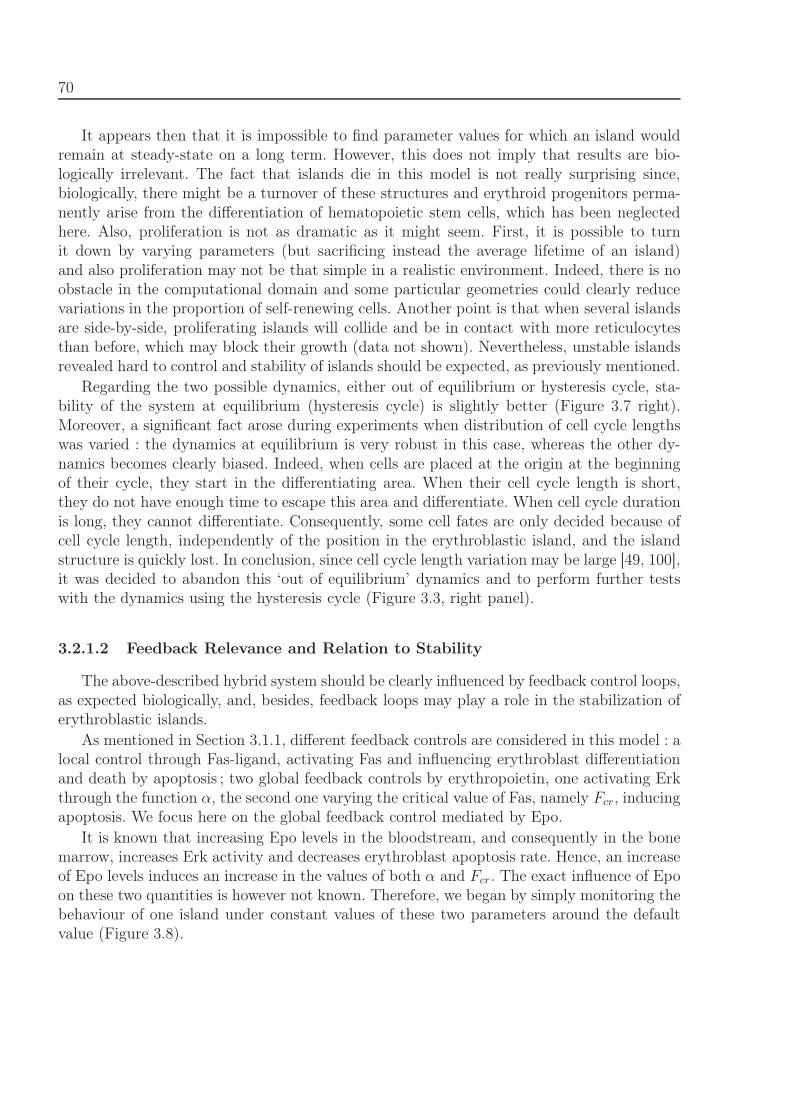
70

It appears then that it is impossible to find parameter values for which an island wouldremain at steady-state on a long term. However, this does not imply that results are bio-logically irrelevant. The fact that islands die in this model is not really surprising since,biologically, there might be a turnover of these structures and erythroid progenitors perma-nently arise from the differentiation of hematopoietic stem cells, which has been neglectedhere. Also, proliferation is not as dramatic as it might seem. First, it is possible to turnit down by varying parameters (but sacrificing instead the average lifetime of an island)and also proliferation may not be that simple in a realistic environment. Indeed, there is noobstacle in the computational domain and some particular geometries could clearly reducevariations in the proportion of self-renewing cells. Another point is that when several islandsare side-by-side, proliferating islands will collide and be in contact with more reticulocytesthan before, which may block their growth (data not shown). Nevertheless, unstable islandsrevealed hard to control and stability of islands should be expected, as previously mentioned.

Regarding the two possible dynamics, either out of equilibrium or hysteresis cycle, sta-bility of the system at equilibrium (hysteresis cycle) is slightly better (Figure 3.7 right).Moreover, a significant fact arose during experiments when distribution of cell cycle lengthswas varied : the dynamics at equilibrium is very robust in this case, whereas the other dy-namics becomes clearly biased. Indeed, when cells are placed at the origin at the beginningof their cycle, they start in the differentiating area. When their cell cycle length is short,they do not have enough time to escape this area and differentiate. When cell cycle durationis long, they cannot differentiate. Consequently, some cell fates are only decided because ofcell cycle length, independently of the position in the erythroblastic island, and the islandstructure is quickly lost. In conclusion, since cell cycle length variation may be large [49, 100],it was decided to abandon this ‘out of equilibrium’ dynamics and to perform further testswith the dynamics using the hysteresis cycle (Figure 3.3, right panel).

3.2.1.2 Feedback Relevance and Relation to Stability

The above-described hybrid system should be clearly influenced by feedback control loops,as expected biologically, and, besides, feedback loops may play a role in the stabilization oferythroblastic islands.

As mentioned in Section 3.1.1, different feedback controls are considered in this model : alocal control through Fas-ligand, activating Fas and influencing erythroblast differentiationand death by apoptosis ; two global feedback controls by erythropoietin, one activating Erkthrough the function α, the second one varying the critical value of Fas, namely Fcr, inducingapoptosis. We focus here on the global feedback control mediated by Epo.

It is known that increasing Epo levels in the bloodstream, and consequently in the bonemarrow, increases Erk activity and decreases erythroblast apoptosis rate. Hence, an increaseof Epo levels induces an increase in the values of both α and Fcr. The exact influence of Epoon these two quantities is however not known. Therefore, we began by simply monitoring thebehaviour of one island under constant values of these two parameters around the defaultvalue (Figure 3.8).

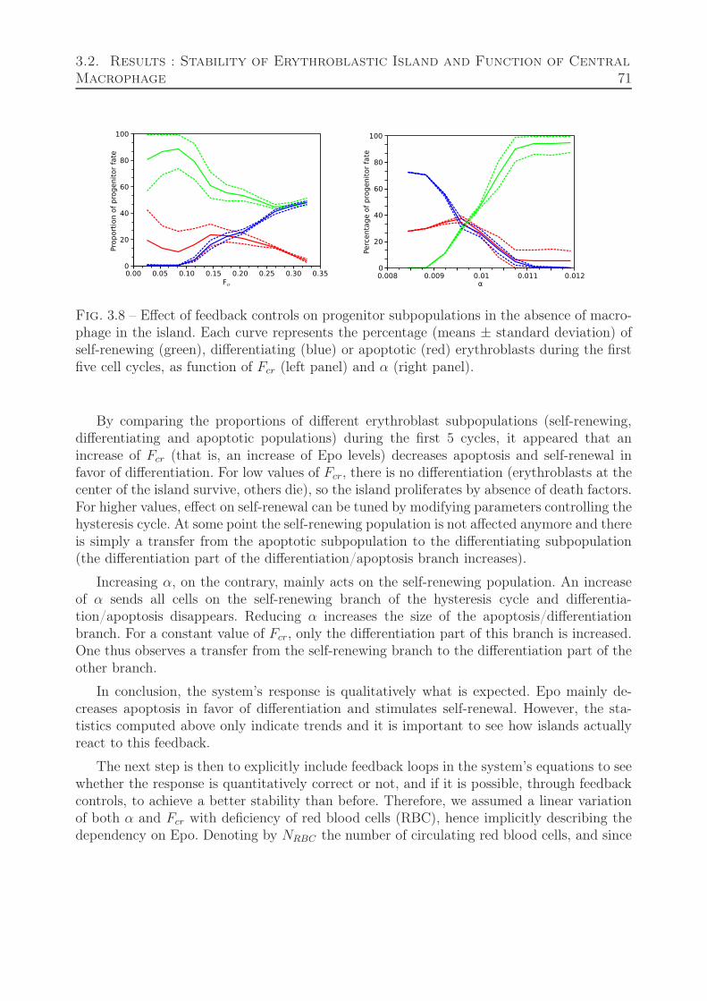
3.2. Results : Stability of Erythroblastic Island and Function of Central

Macrophage 71

0.00 0.05 0.10 0.15 0.20 0.25 0.30 0.35

Prop

ortio

n of

pro

geni

tor f

ate

Fcr

20

0

40

60

80

100

0.008 0.009 0.01 0.011 0.0120

20

40

60

80

100

Perc

enta

geof

prog

enito

rfat

e

α

Fig. 3.8 – Effect of feedback controls on progenitor subpopulations in the absence of macro-phage in the island. Each curve represents the percentage (means ± standard deviation) ofself-renewing (green), differentiating (blue) or apoptotic (red) erythroblasts during the firstfive cell cycles, as function of Fcr (left panel) and α (right panel).

By comparing the proportions of different erythroblast subpopulations (self-renewing,differentiating and apoptotic populations) during the first 5 cycles, it appeared that anincrease of Fcr (that is, an increase of Epo levels) decreases apoptosis and self-renewal infavor of differentiation. For low values of Fcr, there is no differentiation (erythroblasts at thecenter of the island survive, others die), so the island proliferates by absence of death factors.For higher values, effect on self-renewal can be tuned by modifying parameters controlling thehysteresis cycle. At some point the self-renewing population is not affected anymore and thereis simply a transfer from the apoptotic subpopulation to the differentiating subpopulation(the differentiation part of the differentiation/apoptosis branch increases).

Increasing α, on the contrary, mainly acts on the self-renewing population. An increaseof α sends all cells on the self-renewing branch of the hysteresis cycle and differentia-tion/apoptosis disappears. Reducing α increases the size of the apoptosis/differentiationbranch. For a constant value of Fcr, only the differentiation part of this branch is increased.One thus observes a transfer from the self-renewing branch to the differentiation part of theother branch.

In conclusion, the system’s response is qualitatively what is expected. Epo mainly de-creases apoptosis in favor of differentiation and stimulates self-renewal. However, the sta-tistics computed above only indicate trends and it is important to see how islands actuallyreact to this feedback.

The next step is then to explicitly include feedback loops in the system’s equations to seewhether the response is quantitatively correct or not, and if it is possible, through feedbackcontrols, to achieve a better stability than before. Therefore, we assumed a linear variationof both α and Fcr with deficiency of red blood cells (RBC), hence implicitly describing thedependency on Epo. Denoting by NRBC the number of circulating red blood cells, and since

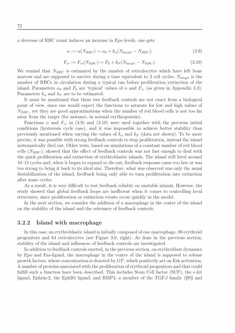
72

a decrease of RBC count induces an increase in Epo levels, one gets

α := α(NRBC) = α0 + kα(Ntarget − NRBC), (3.9)

Fcr := Fcr(NRBC) = F0 + kF (Ntarget − NRBC). (3.10)

We remind that NRBC is estimated by the number of reticulocytes which have left bonemarrow and are supposed to survive during a time equivalent to 3 cell cycles. Ntarget is thenumber of RBCs in circulation during a typical run before proliferation/extinction of theisland. Parameters α0 and F0 are ‘typical’ values of α and Fcr (as given in Appendix 3.3).Parameters kα and kF are to be estimated.

It must be mentioned that these two feedback controls are not exact from a biologicalpoint of view, since one would expect the functions to saturate for low and high values ofNRBC , yet they are good approximations when the number of red blood cells is not too faraway from the target (for instance, in normal erythropoiesis).

Functions α and Fcr in (3.9) and (3.10) were used together with the previous initialconditions (hysteresis cycle case), and it was impossible to achieve better stability thanpreviously mentioned when varying the values of kα and kF (data not shown). To be moreprecise, it was possible with strong feedback controls to stop proliferation, instead the islandsystematically died out. Other tests, based on simulations of a constant number of red bloodcells (NRBC), showed that the effect of feedback controls was not fast enough to deal withthe quick proliferation and extinction of erythroblastic islands. The island still lived around10–15 cycles and, when it began to expand or die out, feedback response came too late or wastoo strong to bring it back to its ideal size. Therefore, what was observed was only the usualdestabilization of the island, feedback being only able to turn proliferation into extinctionafter some cycles.

As a result, it is very difficult to test feedback reliably on unstable islands. However, thestudy showed that global feedback loops are inefficient when it comes to controlling localstructures, since proliferation or extinction events occur quickly in the model.

In the next section, we consider the addition of a macrophage in the center of the islandon the stability of the island and the relevance of feedback controls.

3.2.2 Island with macrophage

In this case, an erythroblastic island is initially composed of one macrophage, 80 erythroidprogenitors and 64 reticulocytes (see Figure 3.6, right). As done in the previous section,stability of the island and influences of feedback controls are investigated.

In addition to feedback controls exerted, in the previous section, on erythroblast dynamicsby Epo and Fas-ligand, the macrophage in the center of the island is supposed to releasegrowth factors, whose concentration is denoted by GF , which positively act on Erk activation.A number of proteins associated with the proliferation of erythroid progenitors and that couldfulfill such a function have been described. This includes Stem Cell factor (SCF), the c-kitligand, Ephrin-2, the EphB4 ligand, and BMP4, a member of the TGFβ family ([95] and

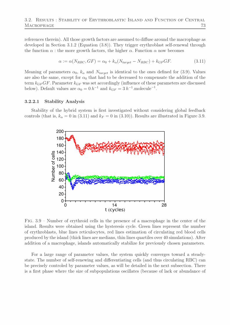
3.2. Results : Stability of Erythroblastic Island and Function of Central

Macrophage 73

references therein). All those growth factors are assumed to diffuse around the macrophage asdeveloped in Section 3.1.2 (Equation (3.8)). They trigger erythroblast self-renewal throughthe function α : the more growth factors, the higher α. Function α now becomes

α := α(NRBC , GF ) = α0 + kα(Ntarget − NRBC) + kGFGF. (3.11)

Meaning of parameters α0, kα and Ntarget is identical to the ones defined for (3.9). Valuesare also the same, except for α0 that had to be decreased to compensate the addition of theterm kGF GF . Parameter kGF was set accordingly (influence of these parameters are discussedbelow). Default values are α0 = 0 h−1 and kGF = 3 h−1.molecule−1.

3.2.2.1 Stability Analysis

Stability of the hybrid system is first investigated without considering global feedbackcontrols (that is, kα = 0 in (3.11) and kF = 0 in (3.10)). Results are illustrated in Figure 3.9.

0 14 280

20

40

60

80

100

120

140

160

180

200

Nu

mb

er

of

ce

lls

t (cycles)

Fig. 3.9 – Number of erythroid cells in the presence of a macrophage in the center of theisland. Results were obtained using the hysteresis cycle. Green lines represent the numberof erythroblasts, blue lines reticulocytes, red lines estimation of circulating red blood cellsproduced by the island (thick lines are medians, thin lines quartiles over 40 simulations). Afteraddition of a macrophage, islands automatically stabilize for previously chosen parameters.

For a large range of parameter values, the system quickly converges toward a steady-state. The number of self-renewing and differentiating cells (and thus circulating RBC) canbe precisely controled by parameter values, as will be detailed in the next subsection. Thereis a first phase where the size of subpopulations oscillates (because of lack or abundance of

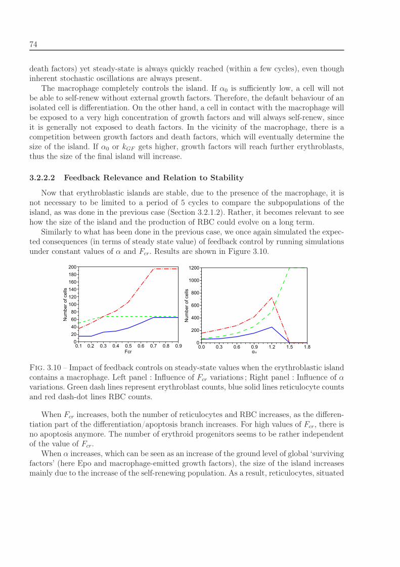
74

death factors) yet steady-state is always quickly reached (within a few cycles), even thoughinherent stochastic oscillations are always present.

The macrophage completely controls the island. If α0 is sufficiently low, a cell will notbe able to self-renew without external growth factors. Therefore, the default behaviour of anisolated cell is differentiation. On the other hand, a cell in contact with the macrophage willbe exposed to a very high concentration of growth factors and will always self-renew, sinceit is generally not exposed to death factors. In the vicinity of the macrophage, there is acompetition between growth factors and death factors, which will eventually determine thesize of the island. If α0 or kGF gets higher, growth factors will reach further erythroblasts,thus the size of the final island will increase.

3.2.2.2 Feedback Relevance and Relation to Stability

Now that erythroblastic islands are stable, due to the presence of the macrophage, it isnot necessary to be limited to a period of 5 cycles to compare the subpopulations of theisland, as was done in the previous case (Section 3.2.1.2). Rather, it becomes relevant to seehow the size of the island and the production of RBC could evolve on a long term.

Similarly to what has been done in the previous case, we once again simulated the expec-ted consequences (in terms of steady state value) of feedback control by running simulationsunder constant values of α and Fcr. Results are shown in Figure 3.10.

0.1 0.90

20406080

100120140160180200

Num

bero

fcel

ls

Fcr0.2 0.3 0.4 0.5 0.6 0.7 0.8 0.0 0.3 0.6 0.9 1.2 1.5 1.8

0

200

400

600

800

1000

1200

α₀

Num

bero

fcel

ls

Fig. 3.10 – Impact of feedback controls on steady-state values when the erythroblastic islandcontains a macrophage. Left panel : Influence of Fcr variations ; Right panel : Influence of αvariations. Green dash lines represent erythroblast counts, blue solid lines reticulocyte countsand red dash-dot lines RBC counts.

When Fcr increases, both the number of reticulocytes and RBC increases, as the differen-tiation part of the differentiation/apoptosis branch increases. For high values of Fcr, there isno apoptosis anymore. The number of erythroid progenitors seems to be rather independentof the value of Fcr.

When α increases, which can be seen as an increase of the ground level of global ‘survivingfactors’ (here Epo and macrophage-emitted growth factors), the size of the island increasesmainly due to the increase of the self-renewing population. As a result, reticulocytes, situated

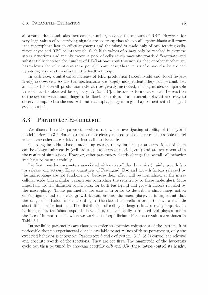
3.3. Parameter Estimation 75

all around the island, also increase in number, as does the amount of RBC. However, forvery high values of α, surviving signals are so strong that almost all erythroblasts self-renew(the macrophage has no effect anymore) and the island is made only of proliferating cells,reticulocyte and RBC counts vanish. Such high values of α may only be reached in extremestress situations and mainly create a pool of cells which may afterwards differentiate andsubstantially increase the number of RBC at once (but this implies that another mechanismhas to lower the value of α at some point). In any case, these values of α may else be avoidedby adding a saturation effect on the feedback loop.

In each case, a substantial increase of RBC production (about 3-fold and 4-fold respec-tively) is observed. As the two mechanisms are largely independent, they can be combinedand thus the overall production rate can be greatly increased, in magnitudes comparableto what can be observed biologically [27, 95, 107]. This seems to indicate that the reactionof the system with macrophage to feedback controls is more efficient, relevant and easy toobserve compared to the case without macrophage, again in good agreement with biologicalevidences [95].

3.3 Parameter Estimation

We discuss here the parameter values used when investigating stability of the hybridmodel in Section 3.2. Some parameters are clearly related to the discrete macroscopic modelwhile some others are related to intracellular dynamics.

Choosing individual-based modelling creates many implicit parameters. Most of themcan be chosen quite easily (cell radius, parameters of motion, etc.) and are not essential inthe results of simulations. However, other parameters clearly change the overall cell behaviorand have to be set carefully.

Let first consider parameters associated with extracellular dynamics (mainly growth fac-tor release and action). Exact quantities of Fas-ligand, Epo and growth factors released bythe macrophage are not fundamental, because their effect will be normalized at the intra-cellular scale (intracellular parameters controlling the sensitivity to these molecules). Moreimportant are the diffusion coefficients, for both Fas-ligand and growth factors released bythe macrophage. These parameters are chosen in order to describe a short range actionof Fas-ligand, and to locate growth factors around the macrophage. It is important thatthe range of diffusion is set according to the size of the cells in order to have a realisticshort-diffusion for instance. The distribution of cell cycle lengths is also really important :it changes how the island expands, how cell cycles are locally correlated and plays a role inthe fate of immature cells when we work out of equilibrium. Parameter values are shown inTable 3.1.

Intracellular parameters are chosen in order to optimize robustness of the system. It isnoticeable that no experimental data is available to set values of these parameters, only theexpected behavior is accessible. Parameters b and c of system (3.1)–(3.2) control the relativeand absolute speeds of the reactions. They are set first. The magnitude of the hysteresiscycle can then be tuned by choosing carefully α/b and β/b (these ratios control its height,

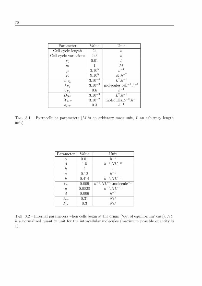
76

Parameter Value UnitCell cycle length 24 h

Cell cycle variations 4/3 hr0 0.01 Lm 1 Mμ 3.105 h−1

K 9.105 M.h−2

DFL3.10−4 L2.h−1

kFL3.10−3 molecules.cell−1.h−1

σFL0.6 h−1

DGF 3.10−3 L2.h−1

WGF 3.10−2 molecules.L−2.h−1

σGF 0.3 h−1

Tab. 3.1 – Extracellular parameters (M is an arbitrary mass unit, L an arbitrary lengthunit)

Parameter Value Unitα 0.01 h−1

β 1.5 h−1.NU−2

k 2 -a 0.12 h−1

b 0.414 h−1.NU−1

kγ 0.009 h−1.NU−1.molecule−1

c 0.0828 h−1.NU−1

d 0.006 h−1

Ecr 0.31 NUFcr 0.3 NU

Tab. 3.2 – Internal parameters when cells begin at the origin (‘out of equilibrium’ case). NUis a normalized quantity unit for the intracellular molecules (maximum possible quantity is1).

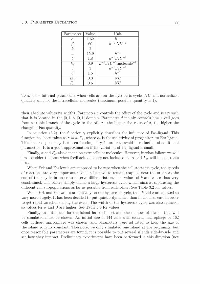
3.3. Parameter Estimation 77

Parameter Value Unitα 1.62 h−1

β 60 h−1.NU−1

k 2 -a 15.9 h−1

b 1.8 h−1.NU−1

kγ 0.9 h−1.NU−2.molecule−1

c 3 h−1.NU−1

d 1.5 h−1

Ecr 0.3 NUFcr 0.6 NU

Tab. 3.3 – Internal parameters when cells are on the hysteresis cycle. NU is a normalizedquantity unit for the intracellular molecules (maximum possible quantity is 1).

their absolute values its width). Parameter a controls the offset of the cycle and is set suchthat it is located in the [0, 1] × [0, 1] domain. Parameter d mainly controls how a cell goesfrom a stable branch of the cycle to the other : the higher the value of d, the higher thechange in Fas quantity.

In equation (3.2), the function γ explicitly describes the influence of Fas-ligand. Thisfunction has been taken as γ = kγFL, where kγ is the sensitivity of progenitors to Fas-ligand.This linear dependency is chosen for simplicity, in order to avoid introduction of additionalparameters. It is a good approximation if the variation of Fas-ligand is small.

Finally, α and Fcr also depend on extracellular molecules. However, in what follows we willfirst consider the case when feedback loops are not included, so α and Fcr will be constantsfirst.

When Erk and Fas levels are supposed to be zero when the cell starts its cycle, the speedsof reactions are very important : some cells have to remain trapped near the origin at theend of their cycle in order to observe differentiation. The values of b and c are thus veryconstrained. The others simply define a large hysteresis cycle which aims at separating thedifferent cell subpopulations as far as possible from each other. See Table 3.2 for values.

When Erk and Fas values are initially on the hysteresis cycle, then b and c are allowed tovary more largely. It has been decided to put quicker dynamics than in the first case in orderto get rapid variations along the cycle. The width of the hysteresis cycle was also reduced,so values for α and β are higher. See Table 3.3 for values.

Finally, an initial size for the island has to be set and the number of islands that willbe simulated must be chosen. An initial size of 144 cells with central macrophage or 162cells without macrophage was chosen, and parameters were adjusted to keep the size ofthe island roughly constant. Therefore, we only simulated one island at the beginning, butonce reasonable parameters are found, it is possible to put several islands side-by-side andsee how they interact. Preliminary experiments have been performed in this direction (not

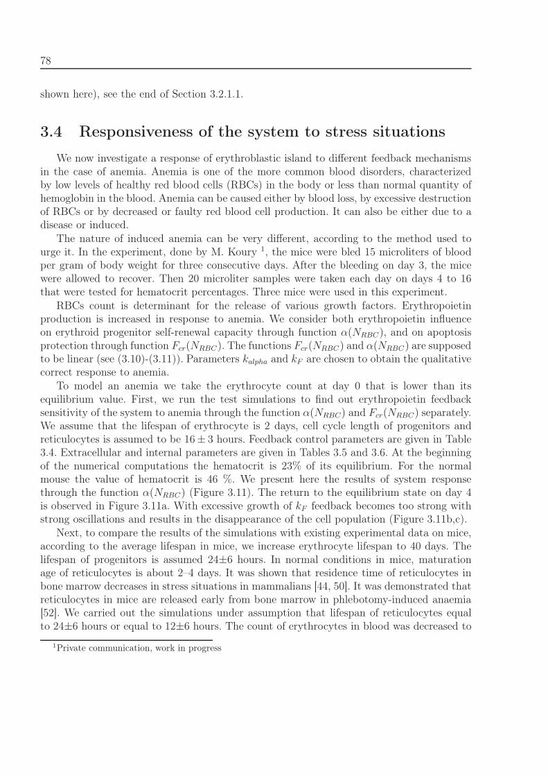
78

shown here), see the end of Section 3.2.1.1.

3.4 Responsiveness of the system to stress situations

We now investigate a response of erythroblastic island to different feedback mechanismsin the case of anemia. Anemia is one of the more common blood disorders, characterizedby low levels of healthy red blood cells (RBCs) in the body or less than normal quantity ofhemoglobin in the blood. Anemia can be caused either by blood loss, by excessive destructionof RBCs or by decreased or faulty red blood cell production. It can also be either due to adisease or induced.

The nature of induced anemia can be very different, according to the method used tourge it. In the experiment, done by M. Koury 1, the mice were bled 15 microliters of bloodper gram of body weight for three consecutive days. After the bleeding on day 3, the micewere allowed to recover. Then 20 microliter samples were taken each day on days 4 to 16that were tested for hematocrit percentages. Three mice were used in this experiment.

RBCs count is determinant for the release of various growth factors. Erythropoietinproduction is increased in response to anemia. We consider both erythropoietin influenceon erythroid progenitor self-renewal capacity through function α(NRBC), and on apoptosisprotection through function Fcr(NRBC). The functions Fcr(NRBC) and α(NRBC) are supposedto be linear (see (3.10)-(3.11)). Parameters kalpha and kF are chosen to obtain the qualitativecorrect response to anemia.

To model an anemia we take the erythrocyte count at day 0 that is lower than itsequilibrium value. First, we run the test simulations to find out erythropoietin feedbacksensitivity of the system to anemia through the function α(NRBC) and Fcr(NRBC) separately.We assume that the lifespan of erythrocyte is 2 days, cell cycle length of progenitors andreticulocytes is assumed to be 16± 3 hours. Feedback control parameters are given in Table3.4. Extracellular and internal parameters are given in Tables 3.5 and 3.6. At the beginningof the numerical computations the hematocrit is 23% of its equilibrium. For the normalmouse the value of hematocrit is 46 %. We present here the results of system responsethrough the function α(NRBC) (Figure 3.11). The return to the equilibrium state on day 4is observed in Figure 3.11a. With excessive growth of kF feedback becomes too strong withstrong oscillations and results in the disappearance of the cell population (Figure 3.11b,c).

Next, to compare the results of the simulations with existing experimental data on mice,according to the average lifespan in mice, we increase erythrocyte lifespan to 40 days. Thelifespan of progenitors is assumed 24±6 hours. In normal conditions in mice, maturationage of reticulocytes is about 2–4 days. It was shown that residence time of reticulocytes inbone marrow decreases in stress situations in mammalians [44, 50]. It was demonstrated thatreticulocytes in mice are released early from bone marrow in phlebotomy-induced anaemia[52]. We carried out the simulations under assumption that lifespan of reticulocytes equalto 24±6 hours or equal to 12±6 hours. The count of erythrocytes in blood was decreased to

1Private communication, work in progress

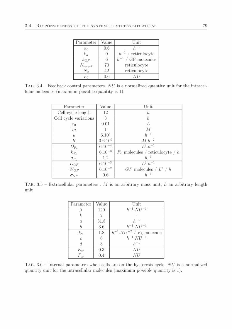
3.4. Responsiveness of the system to stress situations 79

Parameter Value Unitα0 0.6 h−1

kα 0 h−1 / reticulocytekGF 6 h−1 / GF molecules

Ntarget 70 reticulocyteN0 42 reticulocyteF0 0.6 NU

Tab. 3.4 – Feedback control parameters. NU is a normalized quantity unit for the intracel-lular molecules (maximum possible quantity is 1).

Parameter Value UnitCell cycle length 12 h

Cell cycle variations 3 hr0 0.01 Lm 1 Mμ 6.105 h−1

K 3.6.106 M.h−2

DFL6.10−4 L2.h−1

kFL6.10−3 FL molecules / reticulocyte / h

σFL1.2 h−1

DGF 6.10−3 L2.h−1

WGF 6.10−2 GF molecules / L2 / hσGF 0.6 h−1

Tab. 3.5 – Extracellular parameters : M is an arbitrary mass unit, L an arbitrary lengthunit

Parameter Value Unitβ 120 h−1.NU−1

k 2 -a 31.8 h−1

b 3.6 h−1.NU−1

kγ 1.8 h−1.NU−2 / FL moleculec 6 h−1.NU−1

d 3 h−1

Ecr 0.3 NUFcr 0.4 NU

Tab. 3.6 – Internal parameters when cells are on the hysteresis cycle. NU is a normalizedquantity unit for the intracellular molecules (maximum possible quantity is 1).

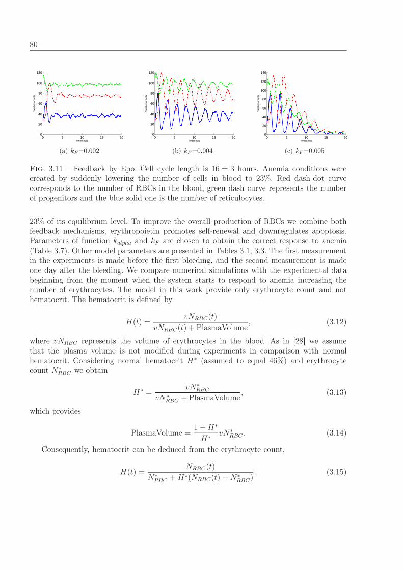
80

0 5 10 15 200

20

40

60

80

100

120

Num

ber

of c

ells

time(days)

(a) kF =0.002

0 5 10 15 200

20

40

60

80

100

120

Num

ber

of c

ells

time(days)

(b) kF =0.004

0 5 10 15 200

20

40

60

80

100

120

140

Num

ber

of c

ells

time(days)

(c) kF =0.005

Fig. 3.11 – Feedback by Epo. Cell cycle length is 16 ± 3 hours. Anemia conditions werecreated by suddenly lowering the number of cells in blood to 23%. Red dash-dot curvecorresponds to the number of RBCs in the blood, green dash curve represents the numberof progenitors and the blue solid one is the number of reticulocytes.

23% of its equilibrium level. To improve the overall production of RBCs we combine bothfeedback mechanisms, erythropoietin promotes self-renewal and downregulates apoptosis.Parameters of function kalpha and kF are chosen to obtain the correct response to anemia(Table 3.7). Other model parameters are presented in Tables 3.1, 3.3. The first measurementin the experiments is made before the first bleeding, and the second measurement is madeone day after the bleeding. We compare numerical simulations with the experimental databeginning from the moment when the system starts to respond to anemia increasing thenumber of erythrocytes. The model in this work provide only erythrocyte count and nothematocrit. The hematocrit is defined by

H(t) =vNRBC(t)

vNRBC(t) + PlasmaVolume, (3.12)

where vNRBC represents the volume of erythrocytes in the blood. As in [28] we assumethat the plasma volume is not modified during experiments in comparison with normalhematocrit. Considering normal hematocrit H∗ (assumed to equal 46%) and erythrocytecount N∗

RBC we obtain

H∗ =vN∗

RBC

vN∗RBC + PlasmaVolume

, (3.13)

which provides

PlasmaVolume =1 − H∗

H∗ vN∗RBC . (3.14)

Consequently, hematocrit can be deduced from the erythrocyte count,

H(t) =NRBC(t)

N∗RBC + H∗(NRBC(t) − N∗

RBC). (3.15)

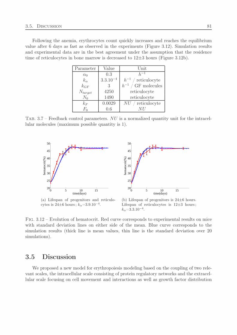
3.5. Discussion 81

Following the anemia, erythrocytes count quickly increases and reaches the equilibriumvalue after 6 days as fast as observed in the experiments (Figure 3.12). Simulation resultsand experimental data are in the best agreement under the assumption that the residencetime of reticulocytes in bone marrow is decreased to 12±3 hours (Figure 3.12b).

Parameter Value Unitα0 0.3 h−1

kα 3.3.10−4 h−1 / reticulocytekGF 3 h−1 / GF molecules

Ntarget 4250 reticulocyteN0 1490 reticulocytekF 0.0029 NU / reticulocyteF0 0.6 NU

Tab. 3.7 – Feedback control parameters. NU is a normalized quantity unit for the intracel-lular molecules (maximum possible quantity is 1).

0 5 10 1520

25

30

35

40

45

50

time(days)

hem

atoc

rit(

%)

(a) Lifespan of progenitors and reticulo-cytes is 24±6 hours ; kα=3.9.10−4.

0 5 10 1520

25

30

35

40

45

50

time(days)

hem

atoc

rit(

%)

(b) Lifespan of progenitors is 24±6 hours.Lifespan of reticulocytes is 12±3 hours ;kα=3.3.10−4.

Fig. 3.12 – Evolution of hematocrit. Red curve corresponds to experimental results on micewith standard deviation lines on either side of the mean. Blue curve corresponds to thesimulation results (thick line is mean values, thin line is the standard deviation over 20simulations).

3.5 Discussion

We proposed a new model for erythropoiesis modeling based on the coupling of two rele-vant scales, the intracellular scale consisting of protein regulatory networks and the extracel-lular scale focusing on cell movement and interactions as well as growth factor distribution

82

in the medium. Description of the competition between two proteins within erythroid proge-nitors has been performed with continuous models (ordinary differential equations) whereascells have been studied as discrete objects on an off-lattice model, so the whole system canbe named ‘hybrid model’, for it consists in the coupling of continuous and discrete systems.Applied to normal erythropoiesis in the bone marrow, in particular to the regulation of ery-throblastic islands, the model suggests an important role of macrophages in the stability ofislands. In the absence of macrophages, erythroblastic islands very quickly lose their stabi-lity, meaning they either die out or abnormally proliferate (with overproduction of erythroidprogenitors). They survive only for the equivalent of about ten cell cycles. On the contrary,when the erythroblastic island is built around a central macrophage, assumed to releasegrowth factors sustaining erythroid progenitor survival and proliferation (like SCF, Ephrin-2or BMP-4 [95]), then the island is a very robust structure, able to produce continuously ery-throcytes while keeping a steady structure (that is an almost constant ratio of reticulocytesover progenitors).

This control of the production of differentiated red blood cells by the macrophage at thelevel of the erythroblastic island may first appear in contradiction with usual knowledge oferythropoiesis. It is indeed well known that during a response to a stress, erythropoiesis isa very intense process, large amounts of cells being produced in a short time, so the wholeprocess is expected to possess the ability to overcome its usual production, in particular theratio of reticulocytes over progenitors should not stay constant. The hypothesis we proposeis that the macrophage, inside the erythroblastic island, controls the explosiveness of ery-thropoiesis and that, contrary to other hematopoietic lineages (white cells, platelets), thiscontrol is necessary because stress erythropoiesis must deal with very large amounts of cellsand otherwise the stability of the process could be lost. It is moreover noticeable that gettingmore stability with the central macrophage does not decrease responsiveness of the model.For instance, the island reacts to perturbations simulating anemia (sudden loss of maturered blood cells), returning quickly to ‘normal’ values of the different erythroid populations,progenitors, reticulocytes and erythrocytes (not shown here). Hence the gain of stabilityis not compensated by a loss in the system’s reactivity. Simulation of stress erythropoiesis(anemia) confirm that the macrophage plays a relevant role in the stability of erythropoiesis.

Some comments may however be made on the behavior of an island without macrophagein its center. Although it is clear that this system cannot lead to a stable island (this can beexplained by considering that fluctuations automatically lead to proliferation or extinction),it is nevertheless possible to imagine a system working with such islands. For instance, ifislands are put side-by-side, proliferation is made difficult (islands cannot expand due toconfinement) and extinction can be compensated by the birth of new islands. Moreover,other assumptions, based on a better knowledge of erythroblastic islands, could lead to morestability (geometry of bone marrow and islands,. . .), even though all scenarii cannot andwere not tested. However, the lack of stability makes it hard to have a clear view on howfeedback controls act on one single island, and as far as we know of, studying erythropoiesismodels (or hematopoiesis models, in a wide sense) without considering feedback controlsdoes not make sense. Hence, searching for island stability appeared relevant in this study. At

3.5. Discussion 83

a global scale, it is still possible that island stability is not necessary and can be compensatedbetween proliferation and extinction. When looking at one single island however, the factthat feedback controls do not work correctly on an unstable island is somewhat compelling.

Stability of the erythroblastic island including a central macrophage was obtained byconsidering two scenarii (see Figure 3.3) for the distribution of Erk and Fas quantities indaughter cells, following mitosis and mother cell’s division. In the first one, initial values ofErk and Fas in newborn cells were set to zero, and cell fate was decided depending on theevolution of concentrations through the cell cycle duration (this is the ‘out of equilibrium’assumption). This scenario was shown to lead to results strongly dependent on the length ofcell cycle. The second scenario, called the ‘hysteresis cycle case’, which is more biologicallyrelevant, consisted in dividing values of Erk and Fas of the mother cell at mitosis into two, soboth daughter cells are located on a hysteresis cycle in the Erk-Fas plane at birth. Combiningthe hysteresis cycle scenario with a structure including a local feedback on the island (themacrophage) gave relevant results and appears very promising. Parameter values which wereobtained through mathematical analysis appear to be very robust and the system exhibitsqualitatively the same behavior for a wide range of parameters. The stability of the islandallows a better control of its size and its subpopulations and, as a result, gives much moresatisfying results on feedback tests.

Regarding parameter values used to study the model and check different scenarii (with orwithout macrophage in the center of the island, distribution of initial quantities of Erk andFas), one must note that most of these values are mainly not accessible through experiments.Some others, such as for instance the time of survival of RBC, are however rather quitearbitrary and not necessarily in agreement with usual knowledge on erythropoiesis. Yet,results show that the behaviour may be satisfying from a biological point of view. Since awide range of parameters is allowed, this system can fit experimental data and numericallyreproduce certain stress behavior.

84

85

Chapitre 4

Pharmacokinetics-Pharmacodynamics

model of leukemia treatment

In this chapter we use the hybrid model to study normal and leukemic red blood cell pro-duction, and treatment of leukemia. Normal cells are supposed to have a circadian rhythm,that influences their cell cycle durations, whereas leukemic cells, appart from being cha-racterized by excessive proliferation and insufficient differentiation and apoptosis, are sup-posed to escape circadian rhythms. We consider a treatment based on periodic adminis-tration of Ara-C, an anti-cancer agent targeting cells in DNA synthesis. A pharmacodyna-mic/pharmacokinetic model of Ara-C is then proposed, and used to simulate the treatment.Influences of the period of the treatment and the day delivery time on the outcome of thetreatment are investigated and stress the relevance of considering chronotherapeutic treat-ments to cure leukemia.

4.1 Mathematical model

4.1.1 Intracellular and extracellular regulation of normal erythro-

poiesis

In this chapter, in order to focus ourself on leukemia treatment we consider two typesof cells, erythroid progenitors and reticulocytes. Reticulocytes produce Fas-ligand whichdiffuses into extracellular matrix and influences erythroid progenitors. Erythroid progenitorsare also influenced by the hormone erythropoietin. Its production depends on the numberof erythrocytes in blood. Finally, we will introduce pharmacokinetics of Ara-C, a drug usedfor chemotherapy of acute myeloblastic leukemia.

Intracellular regulation We focus our attention on two key intracellular proteins, Erkand Fas, which are involved in cell fate decision (high levels of Erk induce cell self-renewal,whereas high levels of Fas induce either cell differentiation or apoptosis). Evolution of the

86

concentrations of these proteins inside an erythroid progenitor is described by a system oftwo ordinary differential equations [29],⎧⎪⎨

⎪⎩dEi

dt= (α(Epo) + βEk

i )(1 − Ei) − aEi − bEiFi,

dFi

dt= γ(FasL)(1 − Fi) − cEiFi − dFi,

(4.1)

where Ei and Fi are the concentrations of Erk and Fas, respectively, in the i-th cell.Here, we do not consider the feedback by erythropoietin. The concentration of Epo is

assumed to be constant, so the function α in (4.1) will be considered as a positive para-meter. For this study, we focus only on the feedback control exerted on progenitor cells byreticulocytes through Fas-ligand (see the next paragraph Extracellular regulation).

As we already discussed above, this system of equations can have between one and threestationary points [29], depending on parameter values. The choice of parameters is an im-portant issue when describing intracellular regulatory networks. In most cases, there are noexperimental data on the reaction rates of involved proteins. So the criterion when choosingparameter values is to describe the normal behavior of the whole system with approximatelycorrect proportion between self-renewing, differentiating and apoptotic cells and the correctresponse of the system to stimulation by the hormones. The set of parameters satisfyingthese conditions may not be unique. A detailed discussion of the choice of parameters ispresented in previous chapter. Here, parameter values are chosen in such a way that thesystem has three steady states, and values are given in Table 4.1. In this case, the systemexhibits bistability, with one unstable steady state, and two stable ones.

Let us recall that the intracellular regulation scheme described above concerns erythroidprogenitors but not reticulocytes. Indeed, reticulocytes are differentiated cells. Similar tomature red blood cells, they do not proliferate. However, reticulocytes produce Fas-ligand,which influences intracellular regulation of erythroid progenitors (the second equation insystem (4.1) depends on Fas-ligand). For large values of Fas-ligand, trajectories of the systemmove towards greater values of Fi and to smaller values of Ei. If during the cell cycle, thevalue of Erk becomes greater than a given critical value Ec, then the cell will self-renew : atthe end of the cell cycle, it will divide and give rise to two daughter cells that are identical tothe mother cell. During the same cell cycle, if the value of Fas becomes greater than a givencritical value, Fc, then the cell immediately dies by apoptosis. If none of these conditions aresatisfied, then the cell will differentiate : when the cell cycle is finished, the cell divides andgives birth to two more mature cells, that are reticulocytes.

Once produced, a reticulocyte remains in the computational domain during a time equalto one cell cycle, during which it produces Fas-ligand, and then becomes a mature ery-throcyte. At the end of their development, reticulocytes leave the bone marrow and enterthe bloodstream as red blood cells. In the framework of our model, reticulocytes that haveperformed one cell cycle are removed from the computational domain.

We note finally that the duration of cell cycle for each cell is considered as a randomvariable with the uniform distribution in the interval [Tc − τ, Tc + τ ], where Tc is the meancell cycle time and τ < Tc is a parameter accounting for variability of the cell cycle duration.

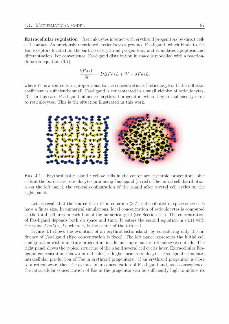
4.1. Mathematical model 87

Extracellular regulation Reticulocytes interact with erythroid progenitors by direct cell-cell contact. As previously mentioned, reticulocytes produce Fas-ligand, which binds to theFas receptors located on the surface of erythroid progenitors, and stimulates apoptosis anddifferentiation. For convenience, Fas-ligand distribution in space is modelled with a reaction-diffusion equation (3.7),

∂FasL

∂t= DΔFasL + W − σFasL,

where W is a source term proportional to the concentration of reticulocytes. If the diffusioncoefficient is sufficiently small, Fas-ligand is concentrated in a small vicinity of reticulocytes.[31]. In this case, Fas-ligand influences erythroid progenitors when they are sufficiently closeto reticulocytes. This is the situation illustrated in this work.

Fig. 4.1 – Erythroblastic island : yellow cells in the center are erythroid progenitors, bluecells at the border are reticulocytes producing Fas-ligand (in red). The initial cell distributionis on the left panel, the typical configuration of the island after several cell cycles on theright panel.

Let us recall that the source term W in equation (3.7) is distributed in space since cellshave a finite size. In numerical simulations, local concentration of reticulocytes is computedas the total cell area in each box of the numerical grid (see Section 2.1). The concentrationof Fas-ligand depends both on space and time. It enters the second equation in (4.1) withthe value FasL(xi, t), where xi is the center of the i-th cell.

Figure 4.1 shows the evolution of an erythroblastic island, by considering only the in-fluence of Fas-ligand (Epo concentration is fixed). The left panel represents the initial cellconfiguration with immature progenitors inside and more mature reticulocytes outside. Theright panel shows the typical structure of the island several cell cycles later. Extracellular Fas-ligand concentration (shown in red color) is higher near reticulocytes. Fas-ligand stimulatesintracellular production of Fas in erythroid progenitors : if an erythroid progenitor is closeto a reticulocyte, then the extracellular concentration of Fas-ligand and, as a consequence,the intracellular concentration of Fas in the progenitor can be sufficiently high to induce its

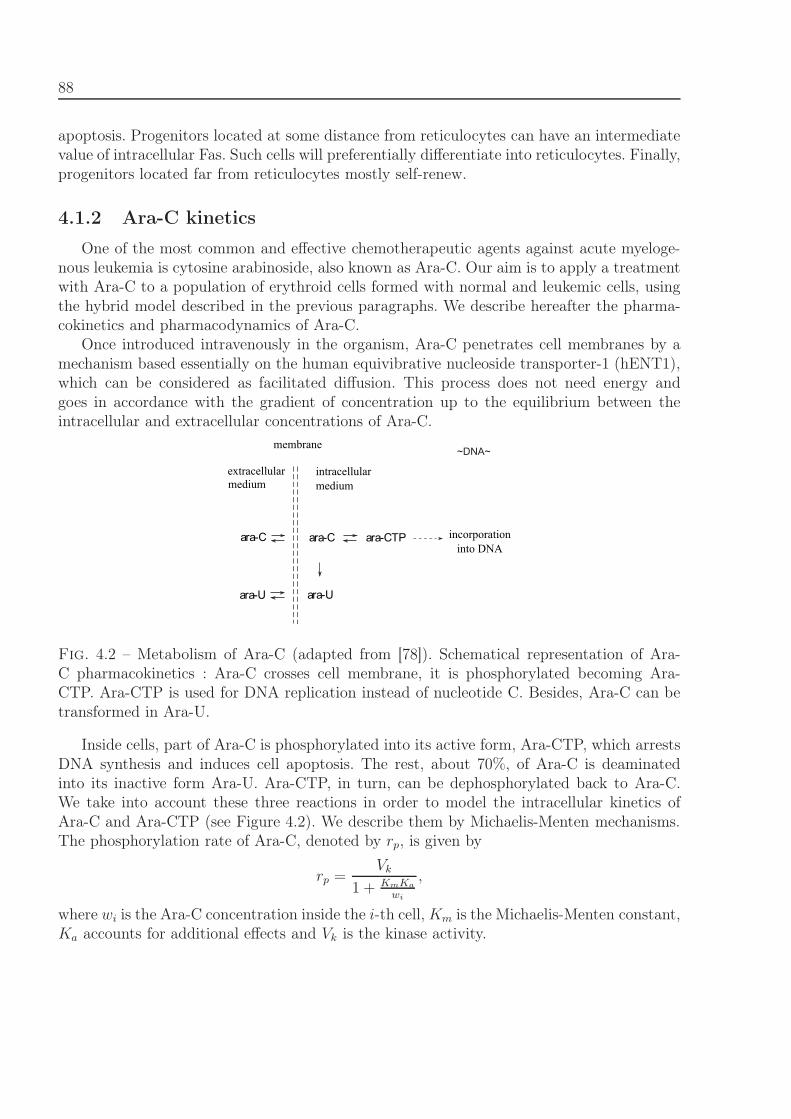
88

apoptosis. Progenitors located at some distance from reticulocytes can have an intermediatevalue of intracellular Fas. Such cells will preferentially differentiate into reticulocytes. Finally,progenitors located far from reticulocytes mostly self-renew.

4.1.2 Ara-C kinetics

One of the most common and effective chemotherapeutic agents against acute myeloge-nous leukemia is cytosine arabinoside, also known as Ara-C. Our aim is to apply a treatmentwith Ara-C to a population of erythroid cells formed with normal and leukemic cells, usingthe hybrid model described in the previous paragraphs. We describe hereafter the pharma-cokinetics and pharmacodynamics of Ara-C.

Once introduced intravenously in the organism, Ara-C penetrates cell membranes by amechanism based essentially on the human equivibrative nucleoside transporter-1 (hENT1),which can be considered as facilitated diffusion. This process does not need energy andgoes in accordance with the gradient of concentration up to the equilibrium between theintracellular and extracellular concentrations of Ara-C.

incorporation into DNA

intracellular medium

extracellular

membrane

ara-C ara-C

ara-U ara-U

ara-CTP

medium

Fig. 4.2 – Metabolism of Ara-C (adapted from [78]). Schematical representation of Ara-C pharmacokinetics : Ara-C crosses cell membrane, it is phosphorylated becoming Ara-CTP. Ara-CTP is used for DNA replication instead of nucleotide C. Besides, Ara-C can betransformed in Ara-U.

Inside cells, part of Ara-C is phosphorylated into its active form, Ara-CTP, which arrestsDNA synthesis and induces cell apoptosis. The rest, about 70%, of Ara-C is deaminatedinto its inactive form Ara-U. Ara-CTP, in turn, can be dephosphorylated back to Ara-C.We take into account these three reactions in order to model the intracellular kinetics ofAra-C and Ara-CTP (see Figure 4.2). We describe them by Michaelis-Menten mechanisms.The phosphorylation rate of Ara-C, denoted by rp, is given by

rp =Vk

1 + KmKa

wi

,

where wi is the Ara-C concentration inside the i-th cell, Km is the Michaelis-Menten constant,Ka accounts for additional effects and Vk is the kinase activity.

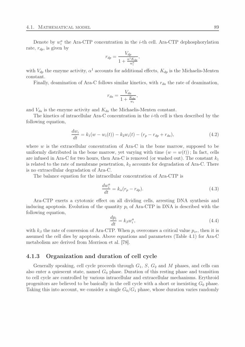
4.1. Mathematical model 89

Denote by wai the Ara-CTP concentration in the i-th cell. Ara-CTP dephosphorylation

rate, rdp, is given by

rdp =Vdp

1 +α1Kdp

wai

,

with Vdp the enzyme activity, α1 accounts for additional effects, Kdp is the Michaelis-Mentenconstant.

Finally, deamination of Ara-C follows similar kinetics, with rda the rate of deamination,

rda =Vda

1 + Kda

wi

,

and Vda is the enzyme activity and Kda the Michaelis-Menten constant.The kinetics of intracellular Ara-C concentration in the i-th cell is then described by the

following equation,

dwi

dt= k1(w − wi(t)) − k2wi(t) − (rp − rdp + rda), (4.2)

where w is the extracellular concentration of Ara-C in the bone marrow, supposed to beuniformly distributed in the bone marrow, yet varying with time (w = w(t)) ; In fact, cellsare infused in Ara-C for two hours, then Ara-C is removed (or washed out). The constant k1

is related to the rate of membrane penetration, k2 accounts for degradation of Ara-C. Thereis no extracellular degradation of Ara-C.

The balance equation for the intracellular concentration of Ara-CTP is

dwai

dt= kα(rp − rdp). (4.3)

Ara-CTP exerts a cytotoxic effect on all dividing cells, arresting DNA synthesis andinducing apoptosis. Evolution of the quantity pi of Ara-CTP in DNA is described with thefollowing equation,

dpi

dt= kβwa

i , (4.4)

with kβ the rate of conversion of Ara-CTP. When pi overcomes a critical value pcr, then it isassumed the cell dies by apoptosis. Above equations and parameters (Table 4.1) for Ara-Cmetabolism are derived from Morrison et al. [78].

4.1.3 Organization and duration of cell cycle

Generally speaking, cell cycle proceeds through G1, S, G2 and M phases, and cells canalso enter a quiescent state, named G0 phase. Duration of this resting phase and transitionto cell cycle are controlled by various intracellular and extracellular mechanisms. Erythroidprogenitors are believed to be basically in the cell cycle with a short or inexisting G0 phase.Taking this into account, we consider a single G0/G1 phase, whose duration varies randomly

90

Tab. 4.1 – Parameter values (N.U. means “no unit”, min is for “minute”)Parameter Value Unit

Force between two cellsH1 Cell compressible part 1.75 μmK Positive parameter 1000

Intracellular regulationα Epo-dependent Erk activation rate 0.0003472 min−1

k Erk self-activation power 2 N.U.β Erk self-activation rate 0.05 min−1

a Erk degradation rate 0.004 min−1

b Erk inhibition constant 0.0138 min−1

kγ Fas-ligand-dependent Fas activation rate 0.0002 min−1

c Fas inhibition rate 0.00138 min−1

d Fas degradation rate 0.0001 min−1

Ec Erk critical level 0.4 N.U.Fc Fas critical level 0.2 N.U.

Extracellular regulationD Fas-ligand diffusion coefficient 1e−5 μm2.min−1

σ Fas-ligand degradation rate 0.02 min−1

W Source term 0.0001 min−1

Metabolism of AraCk1 Membrane penetration rate 0.0116 min−1

k2 Ara-C degradation rate 0 min−1

Vk Kinase activity 1.28 μM.min−1

Km Michaelis-Menten constant 27.0 μMKa Additional effects constant 16 N.U.Vdp Enzyme activity 300 μM.min−1

Kdp Michaelis-Menten constant 900 μMα1 Additional effects constant 44.4 N.U.Vda Enzyme activity 16.45 μM.min−1

Kda Michaelis-Menten constant 1011.7 μMkα Metabolism constant 0.8 N.U.kβ Ara-CTP conversion rate 1 N.U.pcr Critical value of Ara-CTP in DNA 40 μM

Circadian rhythmcx Constant characterizing the circadian clock ∈ [0, 1] N.U.θ Phase shift 5 hours

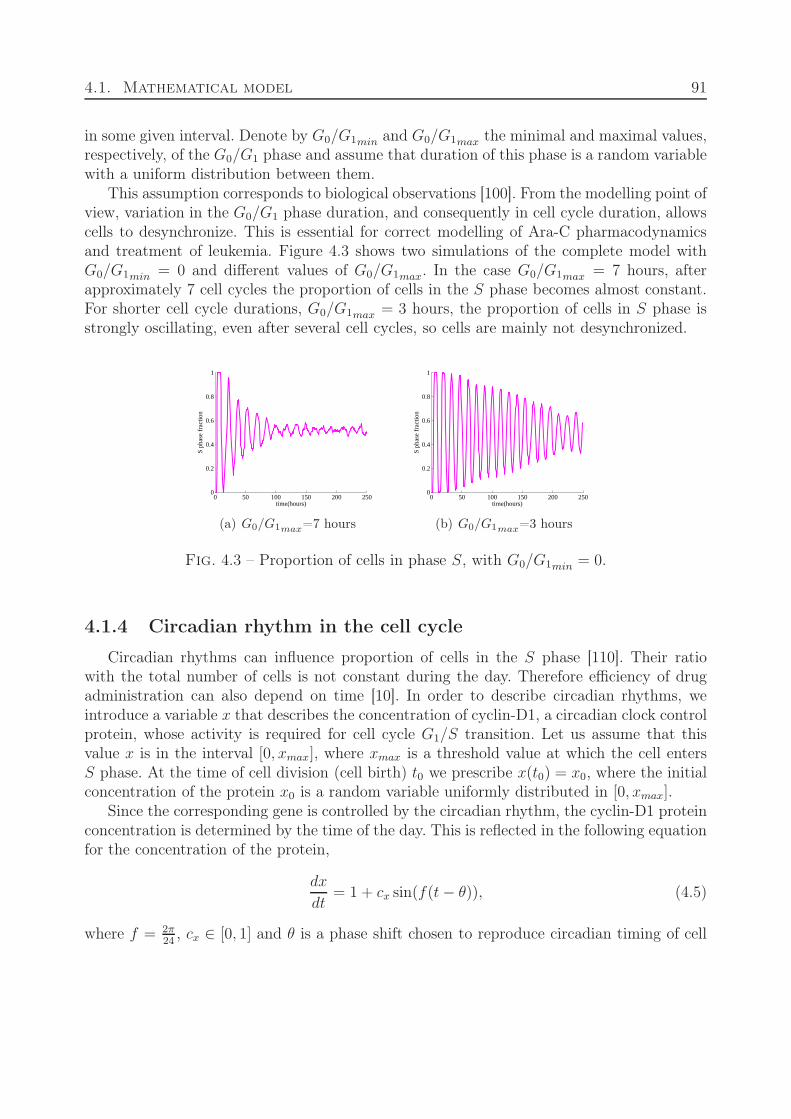
4.1. Mathematical model 91

in some given interval. Denote by G0/G1min and G0/G1max the minimal and maximal values,respectively, of the G0/G1 phase and assume that duration of this phase is a random variablewith a uniform distribution between them.

This assumption corresponds to biological observations [100]. From the modelling point ofview, variation in the G0/G1 phase duration, and consequently in cell cycle duration, allowscells to desynchronize. This is essential for correct modelling of Ara-C pharmacodynamicsand treatment of leukemia. Figure 4.3 shows two simulations of the complete model withG0/G1min = 0 and different values of G0/G1max. In the case G0/G1max = 7 hours, afterapproximately 7 cell cycles the proportion of cells in the S phase becomes almost constant.For shorter cell cycle durations, G0/G1max = 3 hours, the proportion of cells in S phase isstrongly oscillating, even after several cell cycles, so cells are mainly not desynchronized.

0 50 100 150 200 2500

0.2

0.4

0.6

0.8

1

time(hours)

S ph

ase

frac

tion

(a) G0/G1max=7 hours

0 50 100 150 200 2500

0.2

0.4

0.6

0.8

1

time(hours)

S ph

ase

frac

tion

(b) G0/G1max=3 hours

Fig. 4.3 – Proportion of cells in phase S, with G0/G1min = 0.

4.1.4 Circadian rhythm in the cell cycle

Circadian rhythms can influence proportion of cells in the S phase [110]. Their ratiowith the total number of cells is not constant during the day. Therefore efficiency of drugadministration can also depend on time [10]. In order to describe circadian rhythms, weintroduce a variable x that describes the concentration of cyclin-D1, a circadian clock controlprotein, whose activity is required for cell cycle G1/S transition. Let us assume that thisvalue x is in the interval [0, xmax], where xmax is a threshold value at which the cell entersS phase. At the time of cell division (cell birth) t0 we prescribe x(t0) = x0, where the initialconcentration of the protein x0 is a random variable uniformly distributed in [0, xmax].

Since the corresponding gene is controlled by the circadian rhythm, the cyclin-D1 proteinconcentration is determined by the time of the day. This is reflected in the following equationfor the concentration of the protein,

dx

dt= 1 + cx sin(f(t − θ)), (4.5)

where f = 2π24

, cx ∈ [0, 1] and θ is a phase shift chosen to reproduce circadian timing of cell

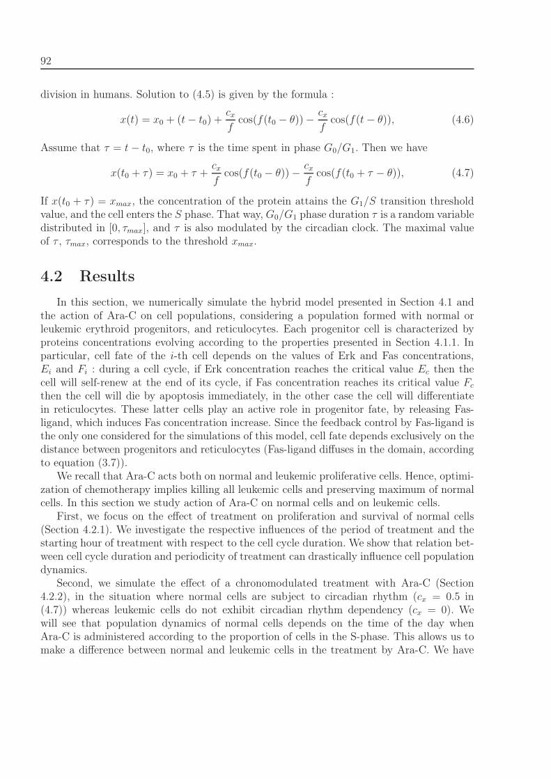
92

division in humans. Solution to (4.5) is given by the formula :

x(t) = x0 + (t − t0) +cx

fcos(f(t0 − θ)) − cx

fcos(f(t − θ)), (4.6)

Assume that τ = t − t0, where τ is the time spent in phase G0/G1. Then we have

x(t0 + τ) = x0 + τ +cx

fcos(f(t0 − θ)) − cx

fcos(f(t0 + τ − θ)), (4.7)

If x(t0 + τ) = xmax, the concentration of the protein attains the G1/S transition thresholdvalue, and the cell enters the S phase. That way, G0/G1 phase duration τ is a random variabledistributed in [0, τmax], and τ is also modulated by the circadian clock. The maximal valueof τ , τmax, corresponds to the threshold xmax.

4.2 Results

In this section, we numerically simulate the hybrid model presented in Section 4.1 andthe action of Ara-C on cell populations, considering a population formed with normal orleukemic erythroid progenitors, and reticulocytes. Each progenitor cell is characterized byproteins concentrations evolving according to the properties presented in Section 4.1.1. Inparticular, cell fate of the i-th cell depends on the values of Erk and Fas concentrations,Ei and Fi : during a cell cycle, if Erk concentration reaches the critical value Ec then thecell will self-renew at the end of its cycle, if Fas concentration reaches its critical value Fc

then the cell will die by apoptosis immediately, in the other case the cell will differentiatein reticulocytes. These latter cells play an active role in progenitor fate, by releasing Fas-ligand, which induces Fas concentration increase. Since the feedback control by Fas-ligand isthe only one considered for the simulations of this model, cell fate depends exclusively on thedistance between progenitors and reticulocytes (Fas-ligand diffuses in the domain, accordingto equation (3.7)).

We recall that Ara-C acts both on normal and leukemic proliferative cells. Hence, optimi-zation of chemotherapy implies killing all leukemic cells and preserving maximum of normalcells. In this section we study action of Ara-C on normal cells and on leukemic cells.

First, we focus on the effect of treatment on proliferation and survival of normal cells(Section 4.2.1). We investigate the respective influences of the period of treatment and thestarting hour of treatment with respect to the cell cycle duration. We show that relation bet-ween cell cycle duration and periodicity of treatment can drastically influence cell populationdynamics.

Second, we simulate the effect of a chronomodulated treatment with Ara-C (Section4.2.2), in the situation where normal cells are subject to circadian rhythm (cx = 0.5 in(4.7)) whereas leukemic cells do not exhibit circadian rhythm dependency (cx = 0). Wewill see that population dynamics of normal cells depends on the time of the day whenAra-C is administered according to the proportion of cells in the S-phase. This allows us tomake a difference between normal and leukemic cells in the treatment by Ara-C. We have

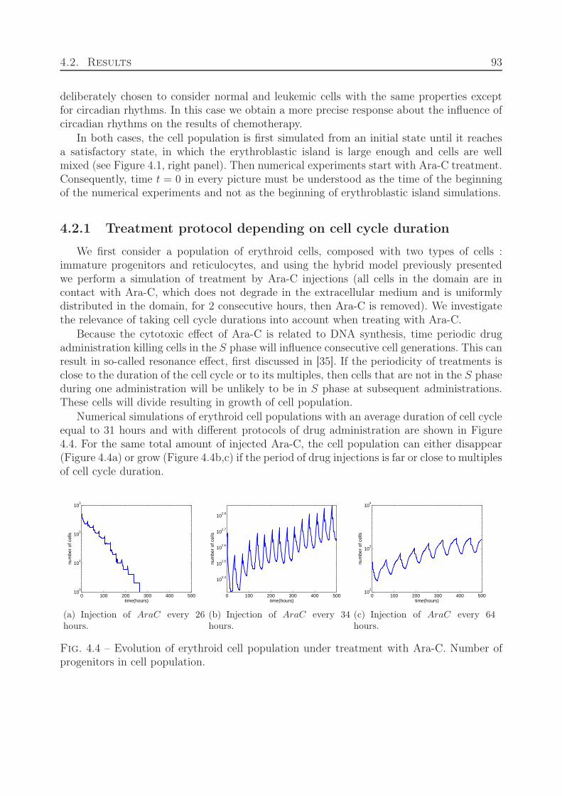
4.2. Results 93

deliberately chosen to consider normal and leukemic cells with the same properties exceptfor circadian rhythms. In this case we obtain a more precise response about the influence ofcircadian rhythms on the results of chemotherapy.

In both cases, the cell population is first simulated from an initial state until it reachesa satisfactory state, in which the erythroblastic island is large enough and cells are wellmixed (see Figure 4.1, right panel). Then numerical experiments start with Ara-C treatment.Consequently, time t = 0 in every picture must be understood as the time of the beginningof the numerical experiments and not as the beginning of erythroblastic island simulations.

4.2.1 Treatment protocol depending on cell cycle duration

We first consider a population of erythroid cells, composed with two types of cells :immature progenitors and reticulocytes, and using the hybrid model previously presentedwe perform a simulation of treatment by Ara-C injections (all cells in the domain are incontact with Ara-C, which does not degrade in the extracellular medium and is uniformlydistributed in the domain, for 2 consecutive hours, then Ara-C is removed). We investigatethe relevance of taking cell cycle durations into account when treating with Ara-C.

Because the cytotoxic effect of Ara-C is related to DNA synthesis, time periodic drugadministration killing cells in the S phase will influence consecutive cell generations. This canresult in so-called resonance effect, first discussed in [35]. If the periodicity of treatments isclose to the duration of the cell cycle or to its multiples, then cells that are not in the S phaseduring one administration will be unlikely to be in S phase at subsequent administrations.These cells will divide resulting in growth of cell population.

Numerical simulations of erythroid cell populations with an average duration of cell cycleequal to 31 hours and with different protocols of drug administration are shown in Figure4.4. For the same total amount of injected Ara-C, the cell population can either disappear(Figure 4.4a) or grow (Figure 4.4b,c) if the period of drug injections is far or close to multiplesof cell cycle duration.

0 100 200 300 400 50010

0

101

102

103

time(hours)

num

ber

of c

ells

(a) Injection of AraC every 26hours.

0 100 200 300 400 500

102.4

102.5

102.6

102.7

102.8

time(hours)

num

ber

of c

ells

(b) Injection of AraC every 34hours.

0 100 200 300 400 50010

2

103

104

time(hours)

num

ber

of c

ells

(c) Injection of AraC every 64hours.

Fig. 4.4 – Evolution of erythroid cell population under treatment with Ara-C. Number ofprogenitors in cell population.

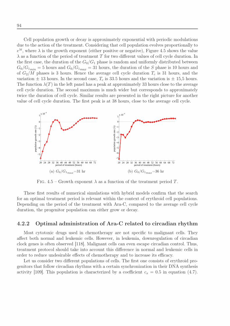
94

Cell population growth or decay is approximately exponential with periodic modulationsdue to the action of the treatment. Considering that cell population evolves proportionally toeλt, where λ is the growth exponent (either positive or negative), Figure 4.5 shows the valueλ as a function of the period of treatment T for two different values of cell cycle duration. Inthe first case, the duration of the G0/G1 phase is random and uniformly distributed betweenG0/G1min = 5 hours and G0/G1max = 31 hours, the duration of the S phase is 10 hours andof G2/M phases is 3 hours. Hence the average cell cycle duration Tc is 31 hours, and thevariation ± 13 hours. In the second case, Tc is 33.5 hours and the variation is ± 15,5 hours.The function λ(T ) in the left panel has a peak at approximately 33 hours close to the averagecell cycle duration. The second maximum is much wider but corresponds to approximatelytwice the duration of cell cycle. Similar results are presented in the right picture for anothervalue of cell cycle duration. The first peak is at 38 hours, close to the average cell cycle.

20 24 28 32 36 40 44 48 52 56 60 64 68 72

−5

−4

−3

−2

−1

0

1x 10

−4

period of treatment (hours)

popu

latio

n gr

owth

rat

e ( λ

)

(a) G0/G1max=31 hr

20 24 28 32 36 40 44 48 52 56 60 64 68 72

−7

−6

−5

−4

−3

−2

−1

0

1x 10

−4

period of treatment (hours)

popu

latio

n gr

owth

rat

e ( λ

)

(b) G0/G1max=36 hr

Fig. 4.5 – Growth exponent λ as a function of the treatment period T .

These first results of numerical simulations with hybrid models confirm that the searchfor an optimal treatment period is relevant within the context of erythroid cell populations.Depending on the period of the treatment with Ara-C, compared to the average cell cycleduration, the progenitor population can either grow or decay.

4.2.2 Optimal administration of Ara-C related to circadian rhythm

Most cytotoxic drugs used in chemotherapy are not specific to malignant cells. Theyaffect both normal and leukemic cells. However, in leukemia, downregulation of circadianclock genes is often observed [118]. Malignant cells can even escape circadian control. Thus,treatment protocol should take into account this difference in normal and leukemic cells inorder to reduce undesirable effects of chemotherapy and to increase its efficacy.

Let us consider two different populations of cells. The first one consists of erythroid pro-genitors that follow circadian rhythms with a certain synchronization in their DNA synthesisactivity [109]. This population is characterized by a coefficient cx = 0.5 in equation (4.7).

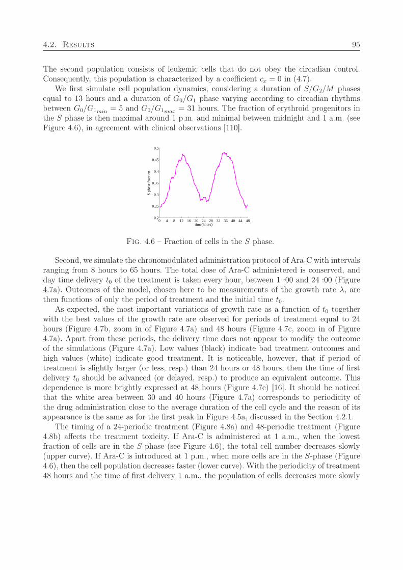
4.2. Results 95

The second population consists of leukemic cells that do not obey the circadian control.Consequently, this population is characterized by a coefficient cx = 0 in (4.7).

We first simulate cell population dynamics, considering a duration of S/G2/M phasesequal to 13 hours and a duration of G0/G1 phase varying according to circadian rhythmsbetween G0/G1min = 5 and G0/G1max = 31 hours. The fraction of erythroid progenitors inthe S phase is then maximal around 1 p.m. and minimal between midnight and 1 a.m. (seeFigure 4.6), in agreement with clinical observations [110].

0 4 8 12 16 20 24 28 32 36 40 44 480.2

0.25

0.3

0.35

0.4

0.45

0.5

time(hours)

S ph

ase

frac

tion

Fig. 4.6 – Fraction of cells in the S phase.

Second, we simulate the chronomodulated administration protocol of Ara-C with intervalsranging from 8 hours to 65 hours. The total dose of Ara-C administered is conserved, andday time delivery t0 of the treatment is taken every hour, between 1 :00 and 24 :00 (Figure4.7a). Outcomes of the model, chosen here to be measurements of the growth rate λ, arethen functions of only the period of treatment and the initial time t0.

As expected, the most important variations of growth rate as a function of t0 togetherwith the best values of the growth rate are observed for periods of treatment equal to 24hours (Figure 4.7b, zoom in of Figure 4.7a) and 48 hours (Figure 4.7c, zoom in of Figure4.7a). Apart from these periods, the delivery time does not appear to modify the outcomeof the simulations (Figure 4.7a). Low values (black) indicate bad treatment outcomes andhigh values (white) indicate good treatment. It is noticeable, however, that if period oftreatment is slightly larger (or less, resp.) than 24 hours or 48 hours, then the time of firstdelivery t0 should be advanced (or delayed, resp.) to produce an equivalent outcome. Thisdependence is more brightly expressed at 48 hours (Figure 4.7c) [16]. It should be noticedthat the white area between 30 and 40 hours (Figure 4.7a) corresponds to periodicity ofthe drug administration close to the average duration of the cell cycle and the reason of itsappearance is the same as for the first peak in Figure 4.5a, discussed in the Section 4.2.1.

The timing of a 24-periodic treatment (Figure 4.8a) and 48-periodic treatment (Figure4.8b) affects the treatment toxicity. If Ara-C is administered at 1 a.m., when the lowestfraction of cells are in the S-phase (see Figure 4.6), the total cell number decreases slowly(upper curve). If Ara-C is introduced at 1 p.m., when more cells are in the S-phase (Figure4.6), then the cell population decreases faster (lower curve). With the periodicity of treatment48 hours and the time of first delivery 1 a.m., the population of cells decreases more slowly

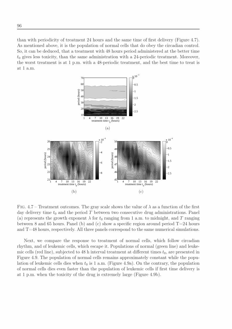
96

than with periodicity of treatment 24 hours and the same time of first delivery (Figure 4.7).As mentioned above, it is the population of normal cells that do obey the circadian control.So, it can be deduced, that a treatment with 48 hours period administered at the better timet0 gives less toxicity, than the same administration with a 24-periodic treatment. Moreover,the worst treatment is at 1 p.m. with a 48-periodic treatment, and the best time to treat isat 1 a.m.

1 4 7 10 13 16 19 2210

20

30

40

50

60

70

treatment time t0 (hours)

peri

od (

hour

s)

−2.5

−2

−1.5

−1

−0.5

0x 10

−3

(a)

treatment time t0 (hours)

peri

od (

hour

s)

1 4 7 10 13 16 19 2221

22

23

24

25

26

−8

−6

−4

−2x 10

−4

(b)

1 4 7 10 13 16 19 2245

46

47

48

49

50

treatment time t0 (hours)

peri

od (

hour

s)

−2.5

−2

−1.5

−1

−0.5

0x 10

−4

(c)

Fig. 4.7 – Treatment outcomes. The gray scale shows the value of λ as a function of the firstday delivery time t0 and the period T between two consecutive drug administrations. Panel(a) represents the growth exponent λ for t0 ranging from 1 a.m. to midnight, and T rangingbetween 8 and 65 hours. Panel (b) and (c) show a specific region around period T=24 hoursand T=48 hours, respectively. All three panels correspond to the same numerical simulations.

Next, we compare the response to treatment of normal cells, which follow circadianrhythm, and of leukemic cells, which escape it. Populations of normal (green line) and leuke-mic cells (red line), subjected to 48 h interval treatment at different times t0, are presented inFigure 4.9. The population of normal cells remains approximately constant while the popu-lation of leukemic cells dies when t0 is 1 a.m. (Figure 4.9a). On the contrary, the populationof normal cells dies even faster than the population of leukemic cells if first time delivery isat 1 p.m. when the toxicity of the drug is extremely large (Figure 4.9b).

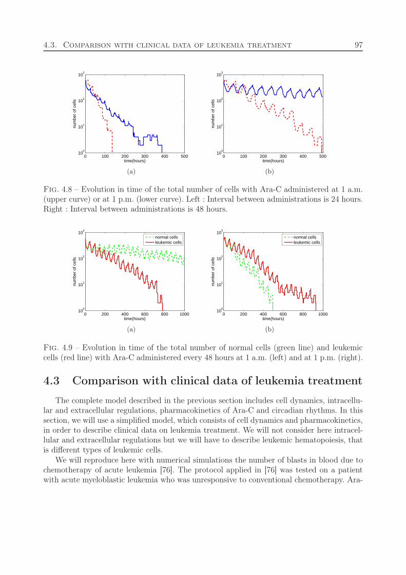
4.3. Comparison with clinical data of leukemia treatment 97

0 100 200 300 400 50010

0

101

102

103

time(hours)

num

ber

of c

ells

(a)

0 100 200 300 400 50010

0

101

102

103

time(hours)

num

ber

of c

ells

(b)

Fig. 4.8 – Evolution in time of the total number of cells with Ara-C administered at 1 a.m.(upper curve) or at 1 p.m. (lower curve). Left : Interval between administrations is 24 hours.Right : Interval between administrations is 48 hours.

0 200 400 600 800 100010

0

101

102

103

time(hours)

num

ber

of c

ells

normal cellsleukemic cells

(a)

0 200 400 600 800 100010

0

101

102

103

time(hours)

num

ber

of c

ells

normal cellsleukemic cells

(b)

Fig. 4.9 – Evolution in time of the total number of normal cells (green line) and leukemiccells (red line) with Ara-C administered every 48 hours at 1 a.m. (left) and at 1 p.m. (right).

4.3 Comparison with clinical data of leukemia treatment

The complete model described in the previous section includes cell dynamics, intracellu-lar and extracellular regulations, pharmacokinetics of Ara-C and circadian rhythms. In thissection, we will use a simplified model, which consists of cell dynamics and pharmacokinetics,in order to describe clinical data on leukemia treatment. We will not consider here intracel-lular and extracellular regulations but we will have to describe leukemic hematopoiesis, thatis different types of leukemic cells.

We will reproduce here with numerical simulations the number of blasts in blood due tochemotherapy of acute leukemia [76]. The protocol applied in [76] was tested on a patientwith acute myeloblastic leukemia who was unresponsive to conventional chemotherapy. Ara-

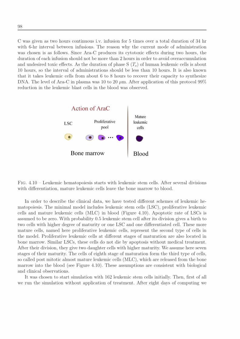
98

C was given as two hours continuous i.v. infusion for 5 times over a total duration of 34 hrwith 6-hr interval between infusions. The reason why the current mode of administrationwas chosen is as follows. Since Ara-C produces its cytotoxic effects during two hours, theduration of each infusion should not be more than 2 hours in order to avoid overaccumulationand undesired toxic effects. As the duration of phase S (Ts) of human leukemic cells is about10 hours, so the interval of administrations should be less than 10 hours. It is also knownthat it takes leukemic cells from about 6 to 8 hours to recover their capacity to synthesizeDNA. The level of Ara-C in plasma was 10 to 20 μm. After application of this protocol 99%reduction in the leukemic blast cells in the blood was observed.

Bone marrow Blood

...LSC Proliferative

pool

Matureleukemic cells

Action of AraC

Fig. 4.10 – Leukemic hematopoiesis starts with leukemic stem cells. After several divisionswith differentiation, mature leukemic cells leave the bone marrow to blood.

In order to describe the clinical data, we have tested different schemes of leukemic he-matopoiesis. The minimal model includes leukemic stem cells (LSC), proliferative leukemiccells and mature leukemic cells (MLC) in blood (Figure 4.10). Apoptotic rate of LSCs isassumed to be zero. With probability 0.5 leukemic stem cell after its division gives a birth totwo cells with higher degree of maturity or one LSC and one differentiated cell. These moremature cells, named here proliferative leukemic cells, represent the second type of cells inthe model. Proliferative leukemic cells at different stages of maturation are also located inbone marrow. Similar LSCs, these cells do not die by apoptosis without medical treatment.After their division, they give two daughter cells with higher maturity. We assume here sevenstages of their maturity. The cells of eighth stage of maturation form the third type of cells,so called post mitotic almost mature leukemic cells (MLC), which are released from the bonemarrow into the blood (see Figure 4.10). These assumptions are consistent with biologicaland clinical observations.

It was chosen to start simulation with 162 leukemic stem cells initially. Then, first of allwe run the simulation without application of treatment. After eight days of computing we

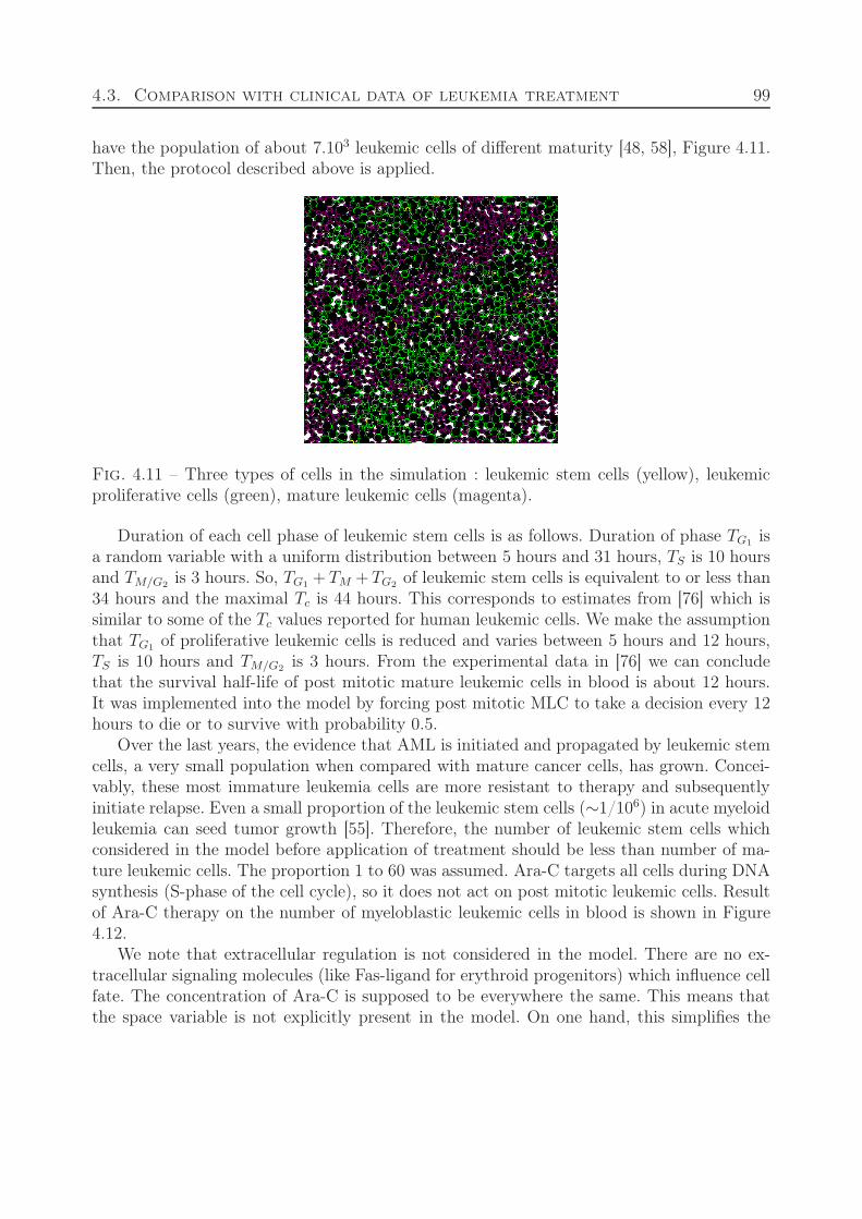
4.3. Comparison with clinical data of leukemia treatment 99

have the population of about 7.103 leukemic cells of different maturity [48, 58], Figure 4.11.Then, the protocol described above is applied.

Fig. 4.11 – Three types of cells in the simulation : leukemic stem cells (yellow), leukemicproliferative cells (green), mature leukemic cells (magenta).

Duration of each cell phase of leukemic stem cells is as follows. Duration of phase TG1 isa random variable with a uniform distribution between 5 hours and 31 hours, TS is 10 hoursand TM/G2

is 3 hours. So, TG1 + TM + TG2 of leukemic stem cells is equivalent to or less than34 hours and the maximal Tc is 44 hours. This corresponds to estimates from [76] which issimilar to some of the Tc values reported for human leukemic cells. We make the assumptionthat TG1 of proliferative leukemic cells is reduced and varies between 5 hours and 12 hours,TS is 10 hours and TM/G2 is 3 hours. From the experimental data in [76] we can concludethat the survival half-life of post mitotic mature leukemic cells in blood is about 12 hours.It was implemented into the model by forcing post mitotic MLC to take a decision every 12hours to die or to survive with probability 0.5.

Over the last years, the evidence that AML is initiated and propagated by leukemic stemcells, a very small population when compared with mature cancer cells, has grown. Concei-vably, these most immature leukemia cells are more resistant to therapy and subsequentlyinitiate relapse. Even a small proportion of the leukemic stem cells (∼1/106) in acute myeloidleukemia can seed tumor growth [55]. Therefore, the number of leukemic stem cells whichconsidered in the model before application of treatment should be less than number of ma-ture leukemic cells. The proportion 1 to 60 was assumed. Ara-C targets all cells during DNAsynthesis (S-phase of the cell cycle), so it does not act on post mitotic leukemic cells. Resultof Ara-C therapy on the number of myeloblastic leukemic cells in blood is shown in Figure4.12.

We note that extracellular regulation is not considered in the model. There are no ex-tracellular signaling molecules (like Fas-ligand for erythroid progenitors) which influence cellfate. The concentration of Ara-C is supposed to be everywhere the same. This means thatthe space variable is not explicitly present in the model. On one hand, this simplifies the

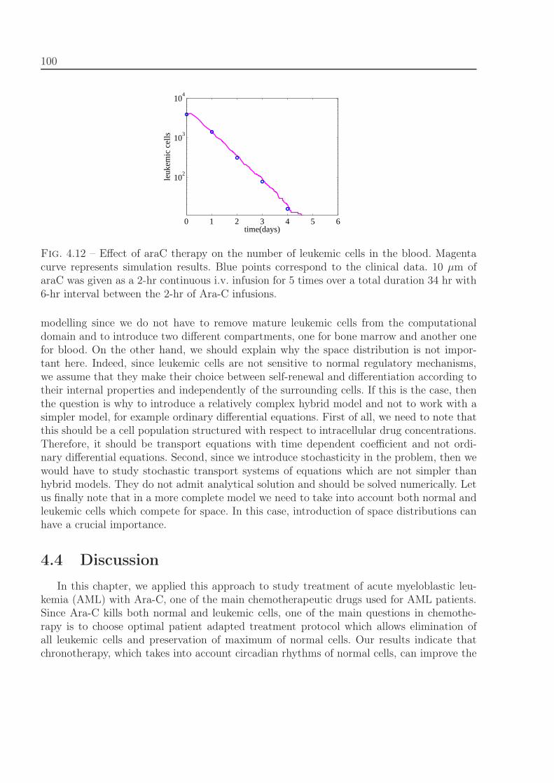
100

0 1 2 3 4 5 6

102

103

104

time(days)

leuk

emic

cel

ls

Fig. 4.12 – Effect of araC therapy on the number of leukemic cells in the blood. Magentacurve represents simulation results. Blue points correspond to the clinical data. 10 μm ofaraC was given as a 2-hr continuous i.v. infusion for 5 times over a total duration 34 hr with6-hr interval between the 2-hr of Ara-C infusions.

modelling since we do not have to remove mature leukemic cells from the computationaldomain and to introduce two different compartments, one for bone marrow and another onefor blood. On the other hand, we should explain why the space distribution is not impor-tant here. Indeed, since leukemic cells are not sensitive to normal regulatory mechanisms,we assume that they make their choice between self-renewal and differentiation according totheir internal properties and independently of the surrounding cells. If this is the case, thenthe question is why to introduce a relatively complex hybrid model and not to work with asimpler model, for example ordinary differential equations. First of all, we need to note thatthis should be a cell population structured with respect to intracellular drug concentrations.Therefore, it should be transport equations with time dependent coefficient and not ordi-nary differential equations. Second, since we introduce stochasticity in the problem, then wewould have to study stochastic transport systems of equations which are not simpler thanhybrid models. They do not admit analytical solution and should be solved numerically. Letus finally note that in a more complete model we need to take into account both normal andleukemic cells which compete for space. In this case, introduction of space distributions canhave a crucial importance.

4.4 Discussion

In this chapter, we applied this approach to study treatment of acute myeloblastic leu-kemia (AML) with Ara-C, one of the main chemotherapeutic drugs used for AML patients.Since Ara-C kills both normal and leukemic cells, one of the main questions in chemothe-rapy is to choose optimal patient adapted treatment protocol which allows elimination ofall leukemic cells and preservation of maximum of normal cells. Our results indicate thatchronotherapy, which takes into account circadian rhythms of normal cells, can improve the

4.4. Discussion 101

result of treatment.

It can be noted that leukemic cells are practically irresponsive to intracellular and ex-tracellular regulation. From the modelling point of view developed in this work, this meansthat the regulation described in Section 4.1.1 does not influence leukemic cells. Hence theanalysis of pharmacokinetics and pharmacodynamics of leukemic cells, which was one of themain objectives of this work, is applicable not only for erythroleukemia but also for all typesof acute leukemia. On the other hand however, when analyzing the influence of chemotherapyon normal cells, we need to take into account their regulation.

Regarding the chronomudulated treatment, it should be noted that resonance is observedin the simplified model while the real in vivo situation can be much more complex. Firstof all, cell lineages with different durations of cell cycle can coexist. Moreover, treatmentitself can change duration of cell cycle, delaying the process of DNA duplication [78]. To ourknowledge, resonance effect has not yet been observed in vivo.

One would have noticed that, in order to use hybrid models and methods in cancermodelling and treatment, development of several submodels are required. First, rather so-phisticated computational tools or frameworks must be developed, including : a) cells asindividual objects that can divide, move, change their type (differentiation), die (disappearfrom the computational domain), interact with each other and with the surrounding mediummechanically and chemically ; b) intracellular regulatory networks described, for instance, byordinary differential equations ; c) extracellular bio-chemical species, whose evolution can bedescribed by partial differential equations. Second, detailed knowledge of intracellular andextracellular regulations are needed. Extracellular regulation can include local regulation dueto cell communication in the tissue or global feedback through hormones or other signalingmolecules produced in other organs. Intracellular and extracellular regulations can influenceeach other in a complex way. Third, pharmacokinetics of medical treatment, treatment pro-tocol, some particular biological or medical aspects of the problem under consideration, likefor instance resonance and chronotherapy in this work, must be modeled.

There are two major obstacles in the development of this approach : values of parametersand availability of clinical data. Some values of parameters can be found in the literature. Inmany cases, however, reaction rates in intracellular protein cascades are completely unknown.Moreover, a “complete” reaction scheme can contain hundreds of interacting proteins, genes,and other factors. So we need to simplify the model preserving its most essential features. Thevalues of parameters should be adjusted in order to obtain biologically realistic functioningof the system : correct proportion of each cell type, correct response to various controlparameters, and so on. The uncertainty of the choice of parameters will nevertheless oftenremain. Pharmacokinetical parameters are taken from [78].

Beyond the question of access to the existing clinical data, which is not straightforward,the main difficulty when trying to compare simulations to existing data, and possibly suggestan improved treatment protocol, is related to the extreme complexity of in vivo processes.Intra-specific variation, which has a crucial importance from the evolutionary point of view,complicates even more treatment optimization for individual patients.

In spite of these difficulties, we can expect that hybrid models will be used in biological

102

experiments and clinical practice. These models allow one to take simultaneously into accountspatial effects, intracellular and extracellular regulation, stochasticity, mechanical propertiesof cells and of the surrounding medium. Conventional continuous models based on ordinaryand partial differential equations either cannot describe ensemble of these effects at all orcan do it in an empiric way hardly possible to justify rigorously. Moreover, they can becomeexcessively complex even for numerical simulations.

103

Chapitre 5

From hybrid to continuous models

The present chapter deals with asymptotic analysis of the diffusion-discrete absorption(DDA) equation. This differential-difference equation describes the steady state diffusionwith the pointwise absorption. Such a model corresponds, for example, to a chain of cells(points) absorbing some substance ; between the cells a steady diffusion process takes place.The discrete sorption corresponds to the term that is a sum of large number of δ-functionsmultiplied by the unknown function (concentration). The main result of of this part of thesisis the homogenization (continualisation) of this equation when the small parameter is thedistance h between two neighboring cells (in the equilibrium state). This homogenizationleads to a purely differential equation describing the macroscopic field. The error estimatesare proved for the difference of the exact solution of the DDA equation and the solution ofthe homogenized differential equation.

Up to our knowledge the existence and uniqueness of solution of the DDA equation wasnot studied earlier. That is why we prove the existence of solution of the DDA equation. Thetheoretical results are confronted to the numerical study. This comparison confirms a goodaccuracy of the asymptotic approximation.

The present chapter continues a set of works devoted to an asymptotic analysis of thediscrete models, in particular, in the atomistic mechanics. Some first results in this directioncan be found in the book [23]. The idea of an asymptotic derivation of the continuousmechanics from the atomistic description has been revisited in a vast literature [62]. Thisapproach is close in some sense to the justification of difference schemes for the partialdifferential equations, when the difference scheme plays part of the initial model and thecorresponding PDE is the limit model. That is why the homogenization of difference schemescould be also considered in the frame of the passage from discrete to continuous models[13, 61, 82, 87]. The discrete homogenization has been developed in [24]. Finally, the hybridpartially discrete and partially continuous models has been considered in [17, 21, 22, 43, 85,86].

104

5.1 Formulation of the problem.

Let R be a positive number, f1 ∈ C([0, 1]), f2 ∈ C([−R, R]), y be a monotone (increa-sing) function [0, 1] → [a, b], such that⎧⎪⎨

⎪⎩y′′(x) = f1(x), x ∈ (0, 1)

y(0) = a,

y(1) = b.

(5.1)

−R < a < b < R ; denote by y−1 the inverse function to y,

χ[a,b](x) =

⎧⎨⎩1, x ∈ [a, b],

0, otherwise.

Consider the problem⎧⎪⎪⎪⎪⎪⎨⎪⎪⎪⎪⎪⎩

u′′(x) − h

k∑j=0

αδ(x − y(jh))u(x) = f2(x), x ∈ (−R, R),

u′(−R) = 0,

u(R) = 0.

(5.2)

where α, h > 0, α is the absorption coefficient, hk = 1 and k is integer.Let us introduce the Sobolev space : H1

0R = {ϕ ∈ H1(−R, R)| ϕ(R) = 0} . Define asolution of (5.2) as a function u ∈ H1

0R, such that ∀ϕ ∈ H10R,

−(

∫ R

−R

u′(x)ϕ′(x)dx +

k∑j=0

αhu(y(jh))ϕ(y(jh))) =

∫ R

−R

f2(x)ϕ(x)dx (5.3)

Theorem 5.1.1 Problem (5.3) admits a unique solution.

Proof

Consider a linear functional : Φ : H10 → R, such that Φ(ϕ) = − ∫ R

−Rfϕdx. This functional

Φ is continuous in L2 : | − ∫ R

−Rfϕdx |≤ ‖f‖L2‖ϕ‖L2 and Φ is also continuous in the norm

‖ϕ′‖L2 due to the Poincaré-Friedrichs inequality. Let us introduce a new scalar product :

(u, v) =

∫ R

−R

u′v′dx + αhk∑

j=0

u(yj)ϕ(yj)

and, respectively, the norm

5.2. Comparison of the discrete and continuous models. 105

‖u‖2 = ‖u′‖2L2

+ αh

k∑j=0

u2(yj). (5.4)

We have

u(yj) = −∫ R

yj

u′(x)dx,

so|u(yj)| ≤

√2R‖u′‖L2,

and

‖u‖2 ≤ (1 + 2αR)‖u′‖2L2

,

because hk = 1. So, the norm (5.4) is equivalent to the norm H10R.

Due to the Riesz theorem, there exists a unique solution u ∈ H10R such that ∀ϕ ∈ H1

0R

Φ(ϕ) =

∫ R

−R

u′v′dx + αhk∑

j=0

u(yj)ϕ(yj)

Here and below, yj = y(jh). Then, there exists a unique u ∈ H10R such that ∀ϕ ∈ H1

0R

−(

∫ R

−R

u′ϕ′dx + αh

k∑j=0

u(y(jh))ϕ(y(jh))) =

∫ R

−R

fϕdx

The theorem is proved.�

The goal of this work is to justify the closeness of problem (5.1)-(5.2) and the macroscopicdifferential equation :⎧⎪⎨

⎪⎩u′′(x) − αu(x)(y−1(x))′χ[a,b](x) = f2(x), x ∈ (−R, R)

u′(−R) = 0,

u(R) = 0.

(5.5)

The existence and uniqueness of its solution is well known.

5.2 Comparison of the discrete and continuous models.

Let us prove that the solution of problems (5.1)-(5.2) and (5.5) satisfy the estimate witha constant c independent of h. To this end, compare the integral

I1 =

∫ x

−R

hk∑

j=1

αu(z)δ(z − y(jh))dz

106

and

I2 =

∫ x

−R

αu(z)(y−1(z))′dz

We have

I1 = h∑

j:y(jh)≤x

αu(y(jh)) = h∑

j:jh≤y−1(x)

αu(y(jh)) =

∫ y−1(x)

0

αu(y(θ))dθ + rh

where

rh =∑

j:j≤ y−1(x)h

∫ jh+h

jh

α[u(y(jh)) − u(y(θ))]dθ +

∫ (j0+1)h

y−1(x)

αu(y(θ))dθ,

where

j0 = [y−1(x)

h]

Applying the Lagrange theorem, we get

|u(y(jh)) − u(y(θ))| ≤ supθ∈[0,1]

|u′(y(θ)||θ − jh| ≤ supx∈[−R,R]

|u′(x)| supθ∈[0,1]

|y′(θ)|h

|∫ (j0+1)h

y−1(x)

αu(y(θ))dθ| ≤ |α| supx∈[−R,R]

|u(x)|h

Hence,

|rh| ≤ Mh,

where

M = α( supx∈[−R,R]

|u′(x)| supθ∈[0,1]

|y′(θ)| + supx∈[−R,R]

|u(x)|) (5.6)

Making change, t = y(θ), in the integral∫ y−1(x)

0αu(y(θ))dθ, we get∫ y−1(x)

0

αu(y(θ))dθ =

∫ x

a

αu(t)(y−1(t))′dt

Integrating equations (5.5) and (5.2), we get⎧⎪⎪⎨⎪⎪⎩

u′(x) −∫ x

−R

h

k∑j=0

αu(θ)δ(θ − y(jh))dθ =

∫ x

−R

f2(θ)dθ,

u(R) = 0.

(5.7)

5.2. Comparison of the discrete and continuous models. 107

⎧⎨⎩ u′(x) −

∫ x

−R

αu(θ)(y−1(θ))′χ[a,b](θ)dθ =

∫ x

−R

f2(θ)dθ,

u(R) = 0.

(5.8)

Denote w = u − u. Then, subtracting (5.7) from (5.8), we get

w′(x) −∫ x

−R

h

k∑j=0

αw(θ)δ(θ − y(jh))dθ + I1 −∫ x

−R

αu(θ)(y−1(θ))′χ[a,b](θ)dθ = 0

On the other hand,

I1 −∫ x

a

αu(t)(y−1(t))′χ[a,b](θ)dθ = rh.

Therefore, ⎧⎪⎪⎨⎪⎪⎩

w′(x) −∫ x

−R

h

k∑j=0

αw(θ)δ(θ − y(jh))dθ + rh = 0,

w(R) = 0.

(5.9)

Multiply (5.9) by ϕ′ where ϕ ∈ H10R(−R, R), and integrate, we get

∫ R

−R

w′ϕ′dx −∫ R

−R

∫ x

−R

h

k∑j=0

αw(θ)δ(θ − y(jh))dθϕ′(x)dx +

∫ R

−R

rh(x)ϕ′(x)dx = 0

∫ R

−R

w′ϕ′dx + h

k∑j=0

αw(y(jh))ϕ(y(jh)) = −∫ R

−R

rh(x)ϕ′(x)dx

Setting ϕ = w, we have

‖w′‖2L2

+ hk∑

j=0

αw2(y(jh)) ≤ ‖rh‖L2‖w′‖L2

‖w′‖L2 ≤ ‖rh‖L2

Applying the Poincaré-Friedrichs inequality, we get

‖w‖H1 ≤√

2R2 + 1‖rh‖L2

Let us estimate constant M (see (5.6)). We have

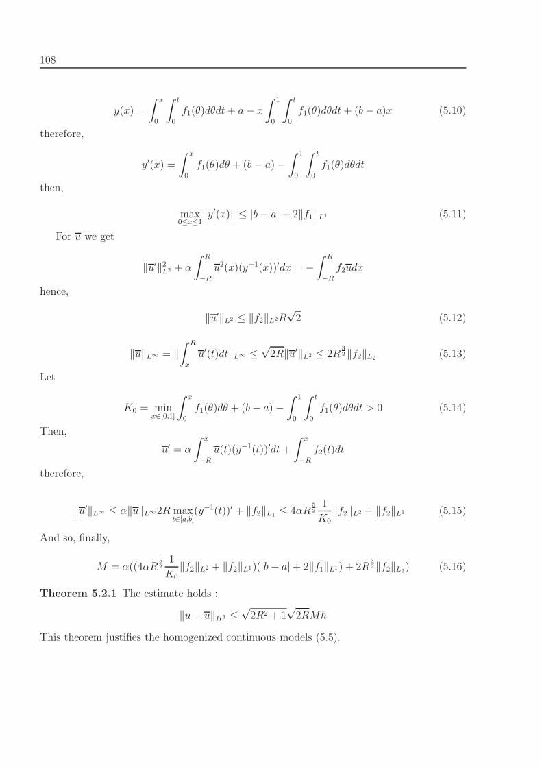
108

y(x) =

∫ x

0

∫ t

0

f1(θ)dθdt + a − x

∫ 1

0

∫ t

0

f1(θ)dθdt + (b − a)x (5.10)

therefore,

y′(x) =

∫ x

0

f1(θ)dθ + (b − a) −∫ 1

0

∫ t

0

f1(θ)dθdt

then,

max0≤x≤1

‖y′(x)‖ ≤ |b − a| + 2‖f1‖L1 (5.11)

For u we get

‖u′‖2L2 + α

∫ R

−R

u2(x)(y−1(x))′dx = −∫ R

−R

f2udx

hence,

‖u′‖L2 ≤ ‖f2‖L2R√

2 (5.12)

‖u‖L∞ = ‖∫ R

x

u′(t)dt‖L∞ ≤√

2R‖u′‖L2 ≤ 2R32‖f2‖L2 (5.13)

Let

K0 = minx∈[0,1]

∫ x

0

f1(θ)dθ + (b − a) −∫ 1

0

∫ t

0

f1(θ)dθdt > 0 (5.14)

Then,

u′ = α

∫ x

−R

u(t)(y−1(t))′dt +

∫ x

−R

f2(t)dt

therefore,

‖u′‖L∞ ≤ α‖u‖L∞2R maxt∈[a,b]

(y−1(t))′ + ‖f2‖L1 ≤ 4αR52

1

K0

‖f2‖L2 + ‖f2‖L1 (5.15)

And so, finally,

M = α((4αR52

1

K0‖f2‖L2 + ‖f2‖L1)(|b − a| + 2‖f1‖L1) + 2R

32‖f2‖L2) (5.16)

Theorem 5.2.1 The estimate holds :

‖u − u‖H1 ≤√

2R2 + 1√

2RMh

This theorem justifies the homogenized continuous models (5.5).

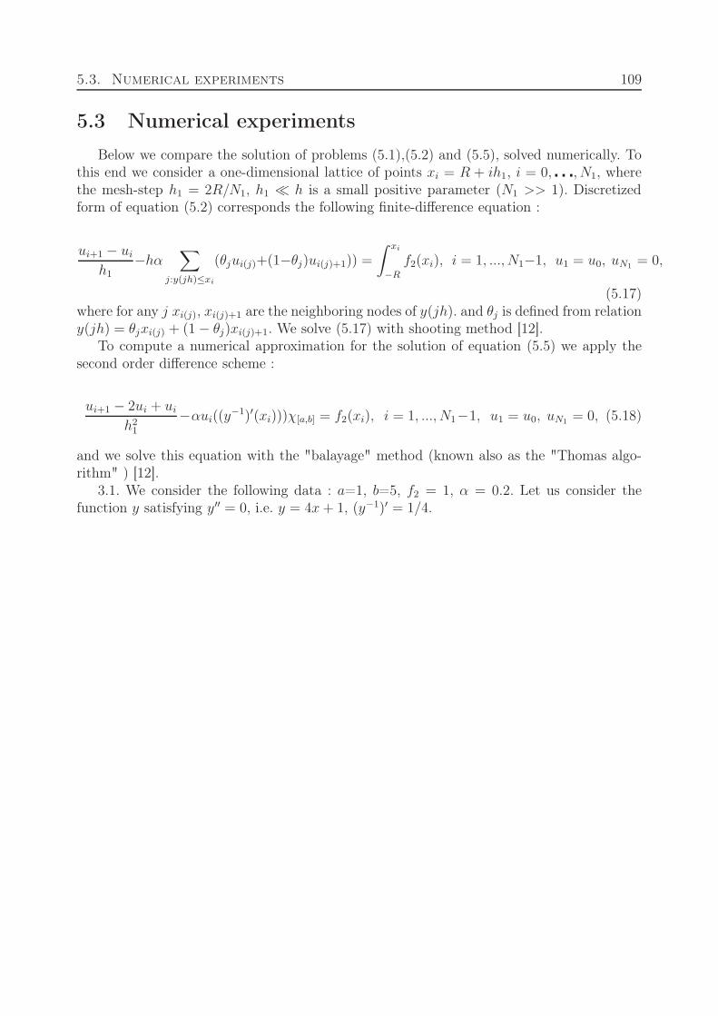
5.3. Numerical experiments 109

5.3 Numerical experiments

Below we compare the solution of problems (5.1),(5.2) and (5.5), solved numerically. Tothis end we consider a one-dimensional lattice of points xi = R + ih1, i = 0, � � �, N1, wherethe mesh-step h1 = 2R/N1, h1 h is a small positive parameter (N1 >> 1). Discretizedform of equation (5.2) corresponds the following finite-difference equation :

ui+1 − ui

h1

−hα∑

j:y(jh)≤xi

(θjui(j)+(1−θj)ui(j)+1)) =

∫ xi

−R

f2(xi), i = 1, ..., N1−1, u1 = u0, uN1 = 0,

(5.17)where for any j xi(j), xi(j)+1 are the neighboring nodes of y(jh). and θj is defined from relationy(jh) = θjxi(j) + (1 − θj)xi(j)+1. We solve (5.17) with shooting method [12].

To compute a numerical approximation for the solution of equation (5.5) we apply thesecond order difference scheme :

ui+1 − 2ui + ui

h21

−αui((y−1)′(xi)))χ[a,b] = f2(xi), i = 1, ..., N1−1, u1 = u0, uN1 = 0, (5.18)

and we solve this equation with the "balayage" method (known also as the "Thomas algo-rithm" ) [12].

3.1. We consider the following data : a=1, b=5, f2 = 1, α = 0.2. Let us consider thefunction y satisfying y′′ = 0, i.e. y = 4x + 1, (y−1)′ = 1/4.

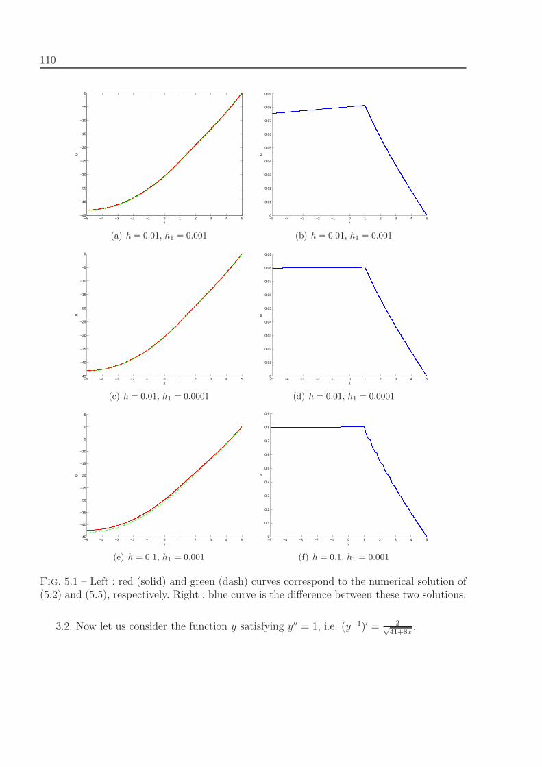
110

−5 −4 −3 −2 −1 0 1 2 3 4 5−45

−40

−35

−30

−25

−20

−15

−10

−5

0

x

U

(a) h = 0.01, h1 = 0.001

−5 −4 −3 −2 −1 0 1 2 3 4 50

0.01

0.02

0.03

0.04

0.05

0.06

0.07

0.08

0.09

x

M

(b) h = 0.01, h1 = 0.001

−5 −4 −3 −2 −1 0 1 2 3 4 5−45

−40

−35

−30

−25

−20

−15

−10

−5

0

x

U

(c) h = 0.01, h1 = 0.0001

−5 −4 −3 −2 −1 0 1 2 3 4 50

0.01

0.02

0.03

0.04

0.05

0.06

0.07

0.08

0.09

x

M

(d) h = 0.01, h1 = 0.0001

−5 −4 −3 −2 −1 0 1 2 3 4 5−45

−40

−35

−30

−25

−20

−15

−10

−5

0

5

x

U

(e) h = 0.1, h1 = 0.001

−5 −4 −3 −2 −1 0 1 2 3 4 50

0.1

0.2

0.3

0.4

0.5

0.6

0.7

0.8

0.9

x

M

(f) h = 0.1, h1 = 0.001

Fig. 5.1 – Left : red (solid) and green (dash) curves correspond to the numerical solution of(5.2) and (5.5), respectively. Right : blue curve is the difference between these two solutions.

3.2. Now let us consider the function y satisfying y′′ = 1, i.e. (y−1)′ = 2√41+8x

.

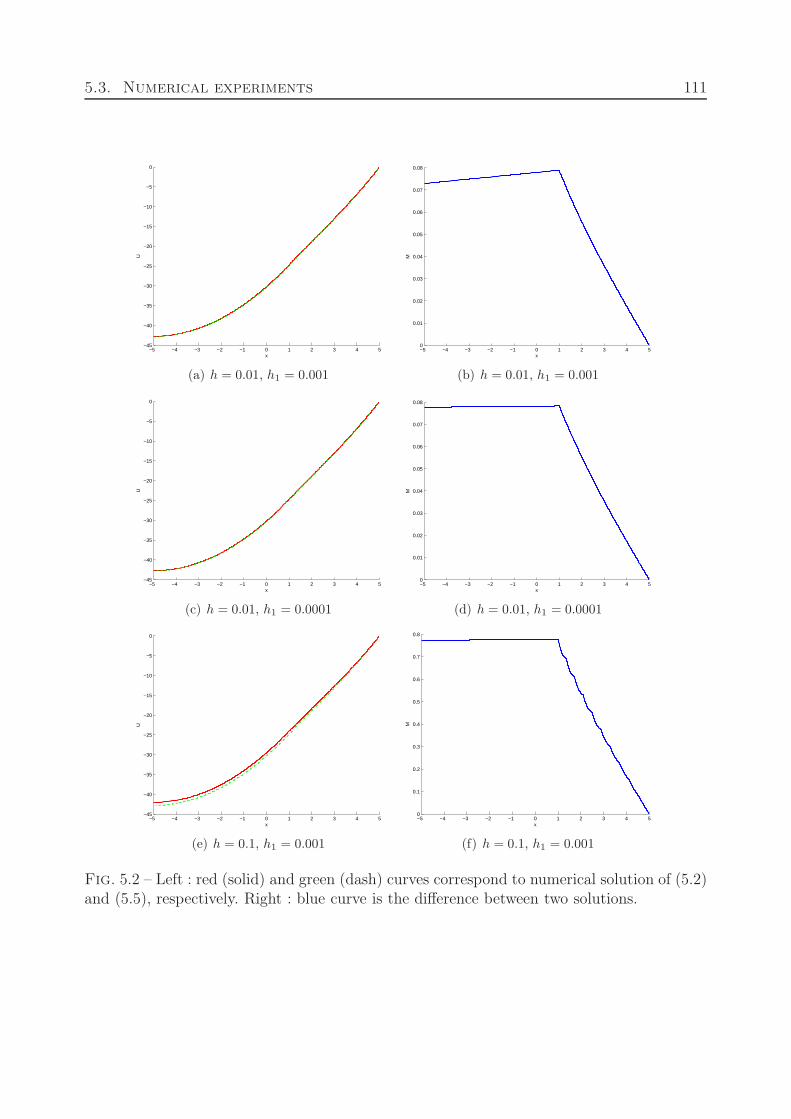
5.3. Numerical experiments 111

−5 −4 −3 −2 −1 0 1 2 3 4 5−45

−40

−35

−30

−25

−20

−15

−10

−5

0

x

U

(a) h = 0.01, h1 = 0.001

−5 −4 −3 −2 −1 0 1 2 3 4 50

0.01

0.02

0.03

0.04

0.05

0.06

0.07

0.08

x

M

(b) h = 0.01, h1 = 0.001

−5 −4 −3 −2 −1 0 1 2 3 4 5−45

−40

−35

−30

−25

−20

−15

−10

−5

0

x

U

(c) h = 0.01, h1 = 0.0001

−5 −4 −3 −2 −1 0 1 2 3 4 50

0.01

0.02

0.03

0.04

0.05

0.06

0.07

0.08

x

M

(d) h = 0.01, h1 = 0.0001

−5 −4 −3 −2 −1 0 1 2 3 4 5−45

−40

−35

−30

−25

−20

−15

−10

−5

0

x

U

(e) h = 0.1, h1 = 0.001

−5 −4 −3 −2 −1 0 1 2 3 4 50

0.1

0.2

0.3

0.4

0.5

0.6

0.7

0.8

x

M

(f) h = 0.1, h1 = 0.001

Fig. 5.2 – Left : red (solid) and green (dash) curves correspond to numerical solution of (5.2)and (5.5), respectively. Right : blue curve is the difference between two solutions.

112

113

Conclusions and Perspectives

Conclusions. This thesis is devoted to off-lattice discrete-continuous hybrid modelingapplied to hematopoiesis and blood diseases, such as leukemia and anemia. The main resultsof the dissertation are as follows :

– Hybrid models with off-lattice cell dynamics were introduced and studied. Cells areconsidered as individual object. Intracellular regulation determine cell fate, that istheir self-renewal, differentiation and apoptosis. Therefore, we do not impose the cor-responding rates as parameters but obtain them as a result of modeling. This is one ofthe main achievements of this work.

– Model examples of hybrid models which describe biological processes such as the com-petition between cell proliferation and apoptosis, between proliferation and differen-tiation and between cell cycling and quiescent state were presented.

– Biological pattern formation with hybrid models and its application to bacteria filamentis discussed.

– A new model of red blood cell production considering the intracellular scale (protein re-gulation, cell fate decision) and the cell population scale (cell-cell interactions, influenceof feedback controls) was proposed.

– The numerical simulation of an erythroblastic island were carried out. Our resultsbrought new information on the role of the macrophage and the erythroblastic islandin the production and regulation of red blood cells, the macrophage was shown to playa key role in the stability and robustness of the production process.

– Using experimental data on anemia in mice, we investigate the roles of different feed-back mechanisms in response to stress situations.

– Hybrid models was applied to leukemia modeling and its treatment. A PhysiologicallyBased Pharmacokinetics-Pharmacodynamics (PBPKPD) model of leukemia treatmentwith AraC drug and the relevance of considering chronotherapeutic treatments tocontrol leukemia was examined.

– The passage from a hybrid model to a continuous model in the 1D case was carriedout :– Comparison between particle dynamics flow and the corresponding equations of

continuum mechanics was done. Numerical simulations confirm a good agreementbetween these approaches

– Comparison of diffusion-discrete absorption equation that describes the steady statediffusion with the pointwise absorption equation and its homogenized form that

114

leads to continuous differential equation shows a good accuracy of the asymptoticapproximation.

Perspectives. We propose and study the model of normal and leukemic erythropoiesiswhich give some insight in the way how erythroid cell proliferation and differentiation canbe controlled, in vitro and in vivo. Nevertheless, further developments could be considered :

– The regulatory network can be completed by introduction of additional proteins, forexample, such as GATA-1, which involved in erythroid progenitor differentiation [2,107].

– Influx of BFU-E and CFU-E from HSC can be considered in the further work.– Both erythropoietin’s influence on erythroid progenitor self-renewal capacity and on

apoptosis protection were taken as linear functions of the number of circulating redblood cells. Saturation effects should be envisaged when confronting the model tostrong perturbations (for instance, a severe anemia), in order to be closer to the realitywhere responses of the organism to a loss of red blood cells have shown to be nonlinear[28, 29].

– In this work focus was made on the behavior of one single erythroblastic island andon feedback controls at global and local scales. However, particular geometries, withobstacles or describing the porous aspect of the bone marrow can be investigated.

– The hybrid model was numerically simulated in two dimensions. The case of simulationsin three dimensions has not been developed. Qualitatively, such a change is not expectedto modify the results, it should nevertheless be tested.

– Moreover, in this work, we focus our attention on red blood cell lineage. Study ofhaematopoiesis should be improved by taking into account development of differentblood cells lineages, lymphopoiesis and myelopoiesis.

– In the modeling of leukemic erythropoiesis and its treatment, in order to predict theoutcome of treatment in a more realistic situation, we need to introduce :– different proliferation rates for normal and leukemic cells– different lineages of leukemic cells– resistance to treatment

– Next important step in the modeling of leukemia treatment will be directed to optimi-zation of the AML treatment by taking into account individual variability of patients.To achieve this goal the malignant cells from individual patients should be analyzed inorder to determine pharmacokinetics-pharmacodynamics parameters.

We intend to study these questions in the subsequent works.

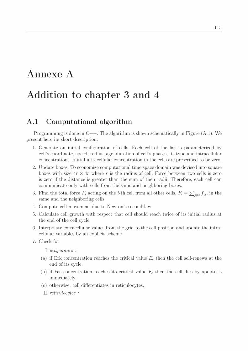
115

Annexe A

Addition to chapter 3 and 4

A.1 Computational algorithm

Programming is done in C++. The algorithm is shown schematically in Figure (A.1). Wepresent here its short description.

1. Generate an initial configuration of cells. Each cell of the list is parameterized bycell’s coordinate, speed, radius, age, duration of cell’s phases, its type and intracellularconcentrations. Initial intracellular concentration in the cells are prescribed to be zero.

2. Update boxes. To economize computational time space domain was devised into squareboxes with size 4r × 4r where r is the radius of cell. Force between two cells is zerois zero if the distance is greater than the sum of their radii. Therefore, each cell cancommunicate only with cells from the same and neighboring boxes.

3. Find the total force Fi acting on the i-th cell from all other cells, Fi =∑

j �=i fij, in thesame and the neighboring cells.

4. Compute cell movement due to Newton’s second law.

5. Calculate cell growth with respect that cell should reach twice of its initial radius atthe end of the cell cycle.

6. Interpolate extracellular values from the grid to the cell position and update the intra-cellular variables by an explicit scheme.

7. Check for

I progenitors :

(a) if Erk concentration reaches the critical value Ec then the cell self-renews at theend of its cycle.

(b) if Fas concentration reaches its critical value Fc then the cell dies by apoptosisimmediately.

(c) otherwise, cell differentiates in reticulocytes.

II reticulocytes :

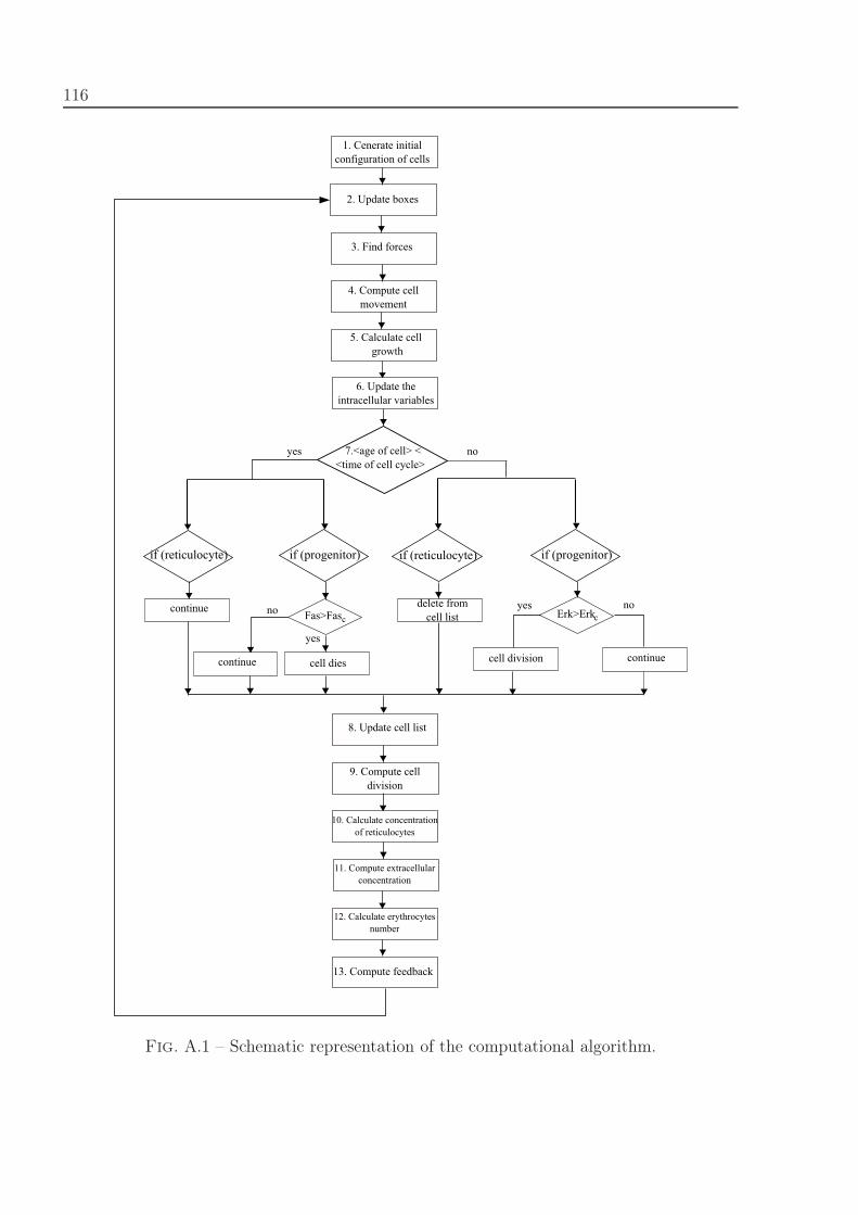
116

1. Cenerate initial configuration of cells

2. Update boxes

3. Find forces

4. Compute cell movement

5. Calculate cell growth

6. Update the intracellular variables

7.<age of cell> < <time of cell cycle>

yes

if (progenitor)

Fas>Fasc

yes

cell dies

if (reticulocyte)

no

if (progenitor)if (reticulocyte)

Erk>Erkcdelete from cell list

cell division

yescontinue

continue

no

8. Update cell list

9. Compute cell division

10. Calculate concentration of reticulocytes

11. Compute extracellular concentration

13. Compute feedback

12. Calculate erythrocytes number

continue

no

Fig. A.1 – Schematic representation of the computational algorithm.

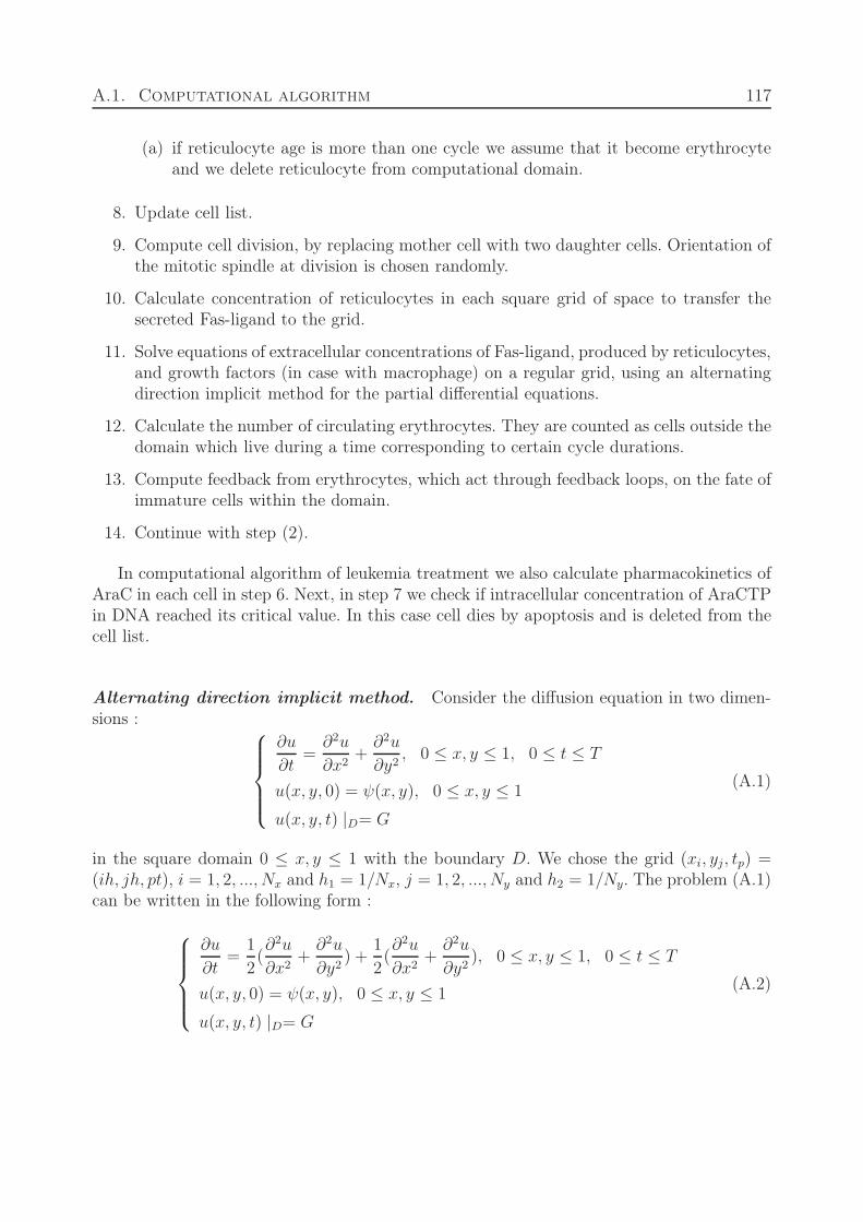
A.1. Computational algorithm 117

(a) if reticulocyte age is more than one cycle we assume that it become erythrocyteand we delete reticulocyte from computational domain.

8. Update cell list.

9. Compute cell division, by replacing mother cell with two daughter cells. Orientation ofthe mitotic spindle at division is chosen randomly.

10. Calculate concentration of reticulocytes in each square grid of space to transfer thesecreted Fas-ligand to the grid.

11. Solve equations of extracellular concentrations of Fas-ligand, produced by reticulocytes,and growth factors (in case with macrophage) on a regular grid, using an alternatingdirection implicit method for the partial differential equations.

12. Calculate the number of circulating erythrocytes. They are counted as cells outside thedomain which live during a time corresponding to certain cycle durations.

13. Compute feedback from erythrocytes, which act through feedback loops, on the fate ofimmature cells within the domain.

14. Continue with step (2).

In computational algorithm of leukemia treatment we also calculate pharmacokinetics ofAraC in each cell in step 6. Next, in step 7 we check if intracellular concentration of AraCTPin DNA reached its critical value. In this case cell dies by apoptosis and is deleted from thecell list.

Alternating direction implicit method. Consider the diffusion equation in two dimen-sions : ⎧⎪⎪⎪⎨

⎪⎪⎪⎩∂u

∂t=

∂2u

∂x2+

∂2u

∂y2, 0 ≤ x, y ≤ 1, 0 ≤ t ≤ T

u(x, y, 0) = ψ(x, y), 0 ≤ x, y ≤ 1

u(x, y, t) |D= G

(A.1)

in the square domain 0 ≤ x, y ≤ 1 with the boundary D. We chose the grid (xi, yj, tp) =(ih, jh, pt), i = 1, 2, ..., Nx and h1 = 1/Nx, j = 1, 2, ..., Ny and h2 = 1/Ny. The problem (A.1)can be written in the following form :

⎧⎪⎪⎪⎨⎪⎪⎪⎩

∂u

∂t=

1

2(∂2u

∂x2+

∂2u

∂y2) +

1

2(∂2u

∂x2+

∂2u

∂y2), 0 ≤ x, y ≤ 1, 0 ≤ t ≤ T

u(x, y, 0) = ψ(x, y), 0 ≤ x, y ≤ 1

u(x, y, t) |D= G

(A.2)

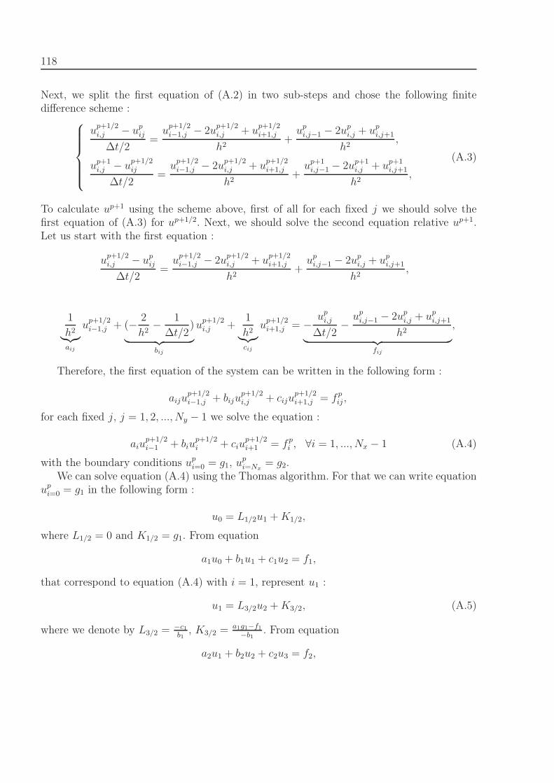
118

Next, we split the first equation of (A.2) in two sub-steps and chose the following finitedifference scheme :⎧⎪⎪⎪⎪⎨

⎪⎪⎪⎪⎩

up+1/2i,j − up

ij

Δt/2=

up+1/2i−1,j − 2u

p+1/2i,j + u

p+1/2i+1,j

h2+

upi,j−1 − 2up

i,j + upi,j+1

h2,

up+1i,j − u

p+1/2ij

Δt/2=

up+1/2i−1,j − 2u

p+1/2i,j + u

p+1/2i+1,j

h2+

up+1i,j−1 − 2up+1

i,j + up+1i,j+1

h2,

(A.3)

To calculate up+1 using the scheme above, first of all for each fixed j we should solve thefirst equation of (A.3) for up+1/2. Next, we should solve the second equation relative up+1.Let us start with the first equation :

up+1/2i,j − up

ij

Δt/2=

up+1/2i−1,j − 2u

p+1/2i,j + u

p+1/2i+1,j

h2+

upi,j−1 − 2up

i,j + upi,j+1

h2,

1

h2︸︷︷︸aij

up+1/2i−1,j + (− 2

h2− 1

Δt/2)︸ ︷︷ ︸

bij

up+1/2i,j +

1

h2︸︷︷︸cij

up+1/2i+1,j = − up

i,j

Δt/2− up

i,j−1 − 2upi,j + up

i,j+1

h2︸ ︷︷ ︸fij

,

Therefore, the first equation of the system can be written in the following form :

aijup+1/2i−1,j + biju

p+1/2i,j + ciju

p+1/2i+1,j = f p

ij ,

for each fixed j, j = 1, 2, ..., Ny − 1 we solve the equation :

aiup+1/2i−1 + biu

p+1/2i + ciu

p+1/2i+1 = f p

i , ∀i = 1, ..., Nx − 1 (A.4)

with the boundary conditions upi=0 = g1, up

i=Nx= g2.

We can solve equation (A.4) using the Thomas algorithm. For that we can write equationup

i=0 = g1 in the following form :

u0 = L1/2u1 + K1/2,

where L1/2 = 0 and K1/2 = g1. From equation

a1u0 + b1u1 + c1u2 = f1,

that correspond to equation (A.4) with i = 1, represent u1 :

u1 = L3/2u2 + K3/2, (A.5)

where we denote by L3/2 = −c1b1

, K3/2 = a1g1−f1

−b1. From equation

a2u1 + b2u2 + c2u3 = f2,

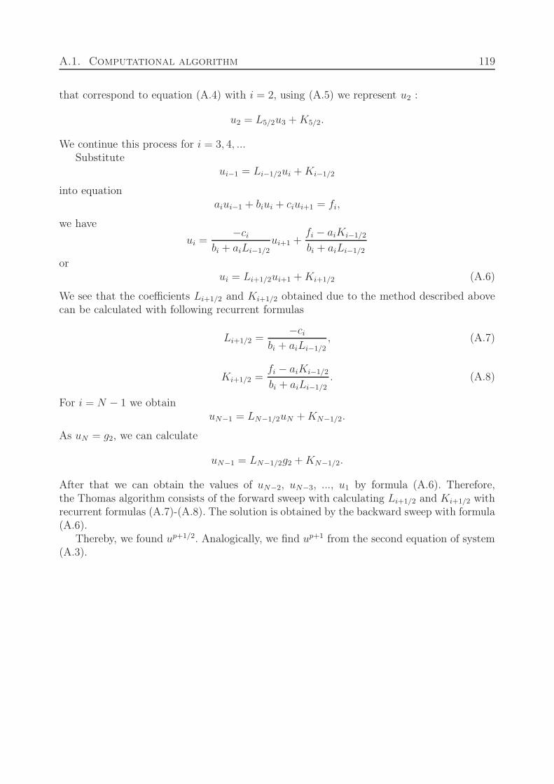
A.1. Computational algorithm 119

that correspond to equation (A.4) with i = 2, using (A.5) we represent u2 :

u2 = L5/2u3 + K5/2.

We continue this process for i = 3, 4, ...Substitute

ui−1 = Li−1/2ui + Ki−1/2

into equationaiui−1 + biui + ciui+1 = fi,

we have

ui =−ci

bi + aiLi−1/2

ui+1 +fi − aiKi−1/2

bi + aiLi−1/2

orui = Li+1/2ui+1 + Ki+1/2 (A.6)

We see that the coefficients Li+1/2 and Ki+1/2 obtained due to the method described abovecan be calculated with following recurrent formulas

Li+1/2 =−ci

bi + aiLi−1/2

, (A.7)

Ki+1/2 =fi − aiKi−1/2

bi + aiLi−1/2

. (A.8)

For i = N − 1 we obtainuN−1 = LN−1/2uN + KN−1/2.

As uN = g2, we can calculate

uN−1 = LN−1/2g2 + KN−1/2.

After that we can obtain the values of uN−2, uN−3, ..., u1 by formula (A.6). Therefore,the Thomas algorithm consists of the forward sweep with calculating Li+1/2 and Ki+1/2 withrecurrent formulas (A.7)-(A.8). The solution is obtained by the backward sweep with formula(A.6).

Thereby, we found up+1/2. Analogically, we find up+1 from the second equation of system(A.3).

120

121

Bibliographie

[1] A.S Ackleh, K. Deng, K. Ito, J. Thibodeaux, A structured erythropoiesis model withnonlinear cell maturation velocity and hormone decay rate, Math. Bios. 204, (2006), pp.21–48.

[2] G.R. Aispuru, M.V. Aguirre, J.A. Aquino-Esperanza, C.N. Lettieri, J.A. Juaristi, N.C.Brandan, Erythroid expansion and survival in response to acute anemia stress : the role ofEPO receptor, GATA-1, Bcl-xL and caspase-3, Cell Biol. Int. 32 (8), (2008), pp. 966–78.

[3] E. Afenya, Acute leukemia and chemotherapy : A modeling viewpoint, Original ResearchArticle Mathematical Biosciences 138 (2), (1996), pp. 79–100.

[4] T. Alarcón, H.M. Byrneb, P.K. Mainia, A cellular automaton model for tumour growthin inhomogeneous environment, J. Theor. Biol. 225, (2003), pp. 257–274.

[5] A.R.A. Anderson, M.A.J. Chaplain, Continuous and discrete mathematical models oftumor-induced angiogenesis, Bull. Math. Biol. 60 (5), (1998), pp. 857–99.

[6] A.R.A. Anderson, M.A.J. Chaplain, K.A. Rejniak, The cellular Potts model and its va-riants, Single-Cell-Based Models in Biology and Medicine, (2007).

[7] A.R.A. Anderson, K.A. Rejniaka, P. Gerleea, V. Quaranta, Modelling of Cancer Growth,Evolution and Invasion : Bridging Scales and Models, Math. Model. Nat. Phenom. 2 (3),(2007), pp. 1–29.

[8] A.R.A. Anderson, A hybrid multiscale model of solid tumour growth and invasion : Evo-lution and the microenvironment, Single Cell Based Models in Biology and Medicine,Mathematics and Biosciences in Interaction, (2007), pp. 3–28.

[9] A. Altinok, F. Lévi and A. Goldbeter, Identifying mechanisms of chronotolerance andchronoefficacy for the anticancer drugs 5-fluorouracil and oxaliplatin by computationalmodeling, Eur. J. Pharm. Sci. 36, (2009), pp. 20–38.

[10] A. Altinok, F. Lévi and A. Goldbeter, A cell cycle automaton model for probing circadianpatterns of anticancer drug delivery, Adv. Drug Deliv. Rev. 59, (2007), pp. 1036-1053.

[11] R. Apostu, M.C. Mackey, Understanding cyclical thrombocytopenia : A mathematicalmodeling approach, J. Theor. Biol. 251, (2008), pp. 297–316.

122

[12] N.S. Bakhvalov, Méthodes Numériques, Edition Mir, Moscow, (1973).

[13] N.S. Bakhvalov, Averaging of partial differential equations with rapidly oscillating coef-ficients, Doklady Acad. Nauk SSSR 224 (2), pp. 351–355, 1975.

[14] A. Bauer, F. Tronche, O. Wessely, C. Kellendonk, H.M. Reichardt, P. Steinlein, G.Schutz, and H. Beug, The glucocorticoid receptor is required for stress erythropoiesis,Genes Dev. 13 (22), (1999), pp. 2996–3002.

[15] S. Bernard , J. Bélair, M.C. Mackey Oscillations in cyclical neutropenia : Newevidence based on mathematical modeling J. Theor. Biol. 223, (2003), pp. 283–298,doi :10.1016/S0022-5193(03)00090-0.

[16] S. Bernard, B. Cajavec Bernard, F. Lévi and H. Herzel, Tumor growth rate deter-mines the timing of optimal chronomodulated treatment schedules, PLoS Comput. Biol.6, (2010), e1000712.

[17] N. Bessonov, V. Volpert, Dynamic models of plant growth.

[18] N. Bessonov , F. Crauste, S. Fischer, P. Kurbatova, V. Volpert, Application of Hy-brid Models to Blood Cell Production in the Bone Marrow, in press Math. Model. Nat.Phenom., submitted.

[19] N. Bessonov, P. Kurbatova, V. Volpert, Particle dynamics modelling of cell populations,Proc. Conf. JANO, Mohhamadia, 2008. Math. Model. Nat. Phenom. 5 (7), (2010), pp.42–47.

[20] N. Bessonov, L. Pujo-Menjouet, V, Volpert. Cell modelling of hematopoiesis. Math.Model. Nat. Phenom. 1 (2), (2006), pp. 81–103.

[21] X. Blanc, C. Le Bris, P.L. Lions, Atomistic to continuum limits for computatioal mate-rials science , Laboratoire Jacques-Louis Lions, (2005).

[22] X. Blanc, C. Le Bris, F. Legoll, Analysis of a prototypical multiscale method couplingatomistic and continuum mechanics, Mathematical Modelling and Numerical Analysis39 (4), (2005), pp. 797–826.

[23] M. Born, K. Huang, Dynamical Theory of Crystal Lattices, Oxford U. P., London, (1954).

[24] D. Caillerie, A. Muorad, A. Raoult, Discrete hohmogenization in graphene sheet mode-ling, Journal of Elasticity 84, (2006), pp. 33–68.

[25] C. Colijn and M.C. Mackey, A mathematical model of hematopoiesis – I. Periodic chronicmyelogenous leukemia, J. Theor. Biol. 237, (2005), pp. 117–132.

[26] C. Colijn and M.C. Mackey, A mathematical model of hematopoiesis – II. Cyclical neu-tropenia, J. Theor. Biol. 237, (2005), pp. 133–146.

BIBLIOGRAPHIE 123

[27] J.A. Chasis and N. Mohandas, Erythroblastic islands : niches for erythropoiesis, Blood112, (2008).

[28] F. Crauste, L. Pujo-Menjouet, S. Génieys, C. Molina, O. Gandrillon, Adding Self-Renewal in Committed Erythroid Progenitors Improves the Biological Relevance of aMathematical Model of Erythropoiesis, J. Theor. Biology 250, (2008), pp. 322–338 .

[29] F. Crauste, I. Demin, O. Gandrillon, V. Volpert, Mathematical study of feedback controlroles and relevance in stress erythropoiesis J. Theor. Biology 263, (2010), pp. 303–316.

[30] S.H. Chapel, P. Veng-Pedersen, R.L. Schmidt, J.A. Widness, A pharmacodynamic ana-lysis of erythropoietin-stimulated reticulocyte response in phlebotomized sheep, J. Phar-macol. Exp. Ther. 295 (1), (2000), pp. 346–351.

[31] R. Cheong, A. Bergmann, S. L. Werner, J. Regal, A. Hoffmann and A. Levchenko,Transient IκB Kinase Activity Mediates Temporal NF-κB Dynamics in Response to aWide Range of Tumor Necrosis Factor-αDoses, The Journal of Biological Chemistry,281 (5), (2006), pp. 2945–2950.

[32] John C. Dallon, Models with lattice-free center-based cells interacting with continuumenvironment variables, Single Cell Based Models in Biology and Medicine, Mathematicsand Biosciences in Interaction, III., (2007), pp. 197–219

[33] J.C. Dallon and H.G. Othmer, A discrete cell model with adaptive signalling for aggre-gation of Dictyostelium discoideum, Philos. Trans. R Soc. Lond B Biol Sci. 352 (1351),(1997), pp. 391–417.

[34] A. Deutsch, Lattice-gas cellular automaton modeling of developing cell systems , Single-Cell-Based Models in Biology and Medicine, Mathematics and Biosciences in Interaction,(2007), pp. 29–51.

[35] B.F. Dibrov, Resonance effect in self-renewing tissues, J. Theor. Biol. 192, (1998), pp.15–33.

[36] S. Dazy, F. Damiola, N. Parisey, H. Beug and O. Gandrillon, The MEK-1/ERKs signa-ling pathway is differentially involved in the self-renewal of early and late avian erythroidprogenitor cells, Oncogene 22, (2003), pp. 9205–9216.

[37] I. Demin, F. Crauste, O. Gandrillon and V. Volpert, A multi-scale model of erythropoie-sis, Journal of Biological Dynamics 4 (2010), pp. 59–70.

[38] R. Dillon, M. Owen, and K. Painter, A single-cell-based model of multicellular growthusing the immersed boundary method, AMS Contemp. Math. 466, (2008), pp. 1–15.

[39] D. Drasdo, Center-based single-cell models : An approach to multi-cellular organizationbased on a conceptual analogy to colloidal particles, Single Cell Based Models in Biologyand Medicine, Mathematics and Biosciences in Interaction, (2007), pp. 171–196

124

[40] S. Dormann and A. Deutsch, Modeling of self-organized avascular tumor growth with ahybrid cellular automaton, In Silico Biol., (2002), pp. 393–406.

[41] J. Eller , I. Gyori, M. Zollei, F. Krizsa, Modelling Thrombopoiesis Regulation - I Modeldescription and simulation results, Comput. Math. Appli 14, (1987), pp. 841–848.

[42] E.H. Estey, Treatment of acute myeloid leukemia, Haematologica, 94 (2009), pp. 10–16

[43] M. Betoue Etoughe, G. Panasenko, Partial homogenization of discrete models, Appli-cable Analysis 87 (12), (2008) pp. 1425–1442.

[44] K.J. Freise, J.A. Widness, R.L. Schmidt, P. Veng-Pedersen, Pharmacodynamic analy-sis of timevariant cellular disposition : reticulocyte disposition changes in phlebotomizedsheep, J. Pharmacokinet. Pharmacodyn. 34, (2007), pp. 519–547.

[45] O. Gandrillon, The v-erbA oncogene. Assessing its differentiation-blocking ability usingnormal chicken erythrocytic progenitor cells, Methods Mol. Biol. 202, (2002), pp. 91–107.

[46] O. Gandrillon , U. Schmidt, H. Beug, J. Samarut, TGF-beta cooperates with TGF-alphato induce the self-renewal of normal erythrocytic progenitors : evidence for an autocrinemechanism, Embo J. 18, (1999), pp. 2764–2781.

[47] C. Giverso, M. Scianna, L. Preziosi, N. Lo Buono and A. Funaro, Individual Cell-BasedModel for In-Vitro Mesothelial Invasion of Ovarian Cancer, Math. Model. Nat. Phenom.5 (1), (2010), pp. 203-223.

[48] D.F. Gluzman, V.A. Nadgornaya, L.M. Sklyarenko, T.S. Ivanovskaya, L.Yu. Polud-nenko, N.I. Ukrainskaya, Immunocytochemical markers in acute leukemias diagnosis,Exp. Oncol., (2010).

[49] A. Golubev, Random discrete competing events vs. dynamic bistable switches in cellproliferation in differentiation, J. Theor. Biol. 267 (3), (2010), pp. 341–354.

[50] R.S. Hillman, Characteristics of marrow production and reticulocyte maturation in nor-mal man in response to anemia, J. Clin. Invest. 48, (1969), pp. 443–453.

[51] S. Hoehme, D. Drasdo, A cell-based simulation software for multi-cellular systems, Bio-informatics 26 (20), (2010), pp. 2641–2642.

[52] N.H. Al-Huniti, J.A. Widness, R.L. Schmidt, P. Veng-Pedersen, Pharmacodynamic ana-lysis of changes in reticulocyte subtype distribution in phlebotomyinduced stress erythro-poiesis, J. Pharmacokinet. Pharmacodyn. 32, (2005), pp. 359–376.

[53] J. Jeon, V. Quaranta, and P. T. Cummings, An Off-Lattice Hybrid Discrete-ContinuumModel of Tumor Growth and Invasion, Biophys. J. 98 (1), (2010), pp. 37–47.

BIBLIOGRAPHIE 125

[54] M. Karttunen, I. Vattulainen, A. Lukkarinen, A novel methods in soft matter simula-tions, Springer, Berlin, (2004).

[55] P. N. Kelly, A. Dakic, J. M. Adams, S. L. Nutt, and A. Strasser, Tumor Growth NeedNot Be Driven by Rare Cancer Stem Cells, Science, 317 (5836), (2007), p. 337.

[56] W. Kern, E. H. Estey, High-dose cytosine arabinoside in the treatment of acute myeloidleukemia Cancer 107, (2006), pp. 116–124.

[57] Y. Kim, M.A. Stolarska, H.G. Othmer, A hybrid model for tumor spheroid growth invitro, I : theoretical development and early results, Math. Models Methods Appl. Sci. 17,(2007), pp. 1773–1798.

[58] H.P. Koeffler, Induction of differentiation of human acute myelogenous leukemia cells :therapeutic implications, Blood 62 (4), (1983), pp. 709–721.

[59] A. Kowal-Vern, F.M. Mazzella, J.D. Cotelingam, M.A. Shrit, J.T. Rector and H.R.Schumacher, Diagnosis and characterization of acute erythroleukemia subsets by deter-mining the percentages of myeloblasts and proerythroblasts in 69 cases, Am. J. Hematol.65, (2000), pp. 5–13.

[60] M. J. Koury and M.C. Bondurant, Erythropoietin retards DNA breakdown and preventsprogrammed death in erythroid progenitor cells, Science 248, (1990), pp. 378–381.

[61] S.M. Kozlov, Averaging of difference schemes, Math. USSR Sb. 57, (1987), pp. 351–369.

[62] I.A. Kunin, Media with Microstructure, Spring-Verlag, Berlin, New-York, I (26), (1982) ;Spring-Verlag, Berlin, New-York, II (44), (1983).

[63] F. Lévi, Circadian chronotherapy for human cancers The Lancet Oncology 2 (5), (2001),pp. 307 – 315.

[64] F. Lévi, C. Focan, A Karaboué, de la Valette V, D. Focan-Henrard, B. Baron, F. Kreutz,S. Giacchetti, Implications of circadian clocks for the rhythmic delivery of cancer thera-peutics, Adv. Drug Deliv. Rev. 59, (2007), pp. 1015–1035.

[65] T.L. Lincoln, P.F. Morrison, J. Aroesty, and G. Carter, em Computer simulation ofleukemia therapy : combined pharmacokinetics, intracellular enzyme kinetics, and cellkinetics of the treatment of l1210 leukemia by cytosine arabinoside, Cancer Treat. Rep.60, (1976), pp. 1723–1739.

[66] A. Madan, C. Lin, Z. Wang and P.T. Curtin, Autocrine stimulation by erythropoietinin transgenic mice results in erythroid proliferation without neoplastic transformation,Blood Cells, Molecules and Diseases, 30 (2003), pp. 82–89.

126

[67] J.M. Mahaffy, J. Belair, M.C. Mackey, em Hematopoietic model with moving boundarycondition and state dependent delay : applications in erythropoiesis, J. Theor. Biol. 190,(1998), pp. 135–146.

[68] F.M. Mazzella, C. Alvares, A. Kowal-Vern and H.R. Schumacher, The acute erythroleu-kemias, Clin. Lab. Med. 20, (2000), pp. 119–37.

[69] M.C. Mackey, Unified hypothesis of the origin of aplastic anaemia and periodic hema-topoïesis, Blood 51, (1978), pp. 941–956.

[70] M.C Mackey, Dynamic hematological disorders of stem cell origin, In : G. Vassileva-Popova and E. V. Jensen, Editors. Biophysical and Biochemical Information Transfer inRecognition, Plenum Press, New York., (1979), pp. 373–409.

[71] M.C. Mackey, R. Rudnicki, A new criterion for the global stability of simultaneous cellreplication and maturation processes, J. Math. Biol. 38, (1999), pp. 195–219.

[72] S.R. McDougall, A.R.A. Anderson, M.A.J. Chaplain and J.A. Sherratt, Mathematicalmodelling of flow through vascular networks : Implications for tumour-induced angioge-nesis and chemotherapy strategies, Bulletin of Mathematical Biology 64 (4), (2002), pp.673–702.

[73] F. Michor, T.P. Hughes, Y. Iwasa, S. Branford, N.P. Shah, et al. Dynamics of chronicmyeloid leukaemia, Nature 435 (7046), (2005), pp. 1267–1270.

[74] F. Michor, Quantitative approaches to analyzing imatinib-treated chronic myeloid leu-kemia, Trends Pharmacol. Sci. 28 (5), (2007), pp. 197–199.

[75] F. Michor, Mathematical models of cancer stem cells, J. Clin. Oncol. 26 (17), (2008),pp. 2854–1861.

[76] R.L. Momparler, A Model for the Chemotherapy of Acute Leukemia with 1-β-D-Arabinofuranosylcytosine, Cancer Research 34, (1974), pp. 1775–1787.

[77] M.C. Mormont and F. Lévi, Cancer chronotherapy : principles, applications, and pers-pectives, Cancer 97, (2003), pp. 155–69.

[78] P.F. Morrison, T.L. Lincoln and J. Aroesty, The disposition of ara-c and its metabolites :a pharmacokinetic simulation, Cancer Chemother. Rep. 59, (1975), pp. 861–876.

[79] R. De Maria, U. Testa, L. Luchetti, A. Zeuner, G. Stassi, E. Pelosi, R. Riccioni, N. Felli,P. Samoggia and C. Peschle, Apoptotic Role of Fas/Fas Ligand System in the Regulationof Erythropoiesis, Blood 93, (1999), pp. 796–803.

[80] Y. Nagata, N. Takahashi, R.J. Davis, K. Todokoro, Activation of p38 MAP kinase andJNK but not ERK is required for erythropoietin-induced erythroid differentiation Blood92, (1998), pp. 1859–1869.

BIBLIOGRAPHIE 127

[81] H. G. Othmer, K. Painter, D. Umulis,C. Xue, The Intersection of Theory and Appli-cation in Elucidating Pattern Formation in Developmental Biology, Math. Model. Nat.Phenom. 4 (4), (2009), pp. 3–82.

[82] R. Orive, E. Zuazua, Finite difference approximation of homogenization problems forelliptic equations, Multi-scale Methodes and Simulation 4, (2005), pp. 36–87.

[83] J.M. Osborne, A. Walter, S.K. Kershaw, G.R. Mirams, A.G. Fletcher, P. Pathmanathan,D. Gavaghan, O.E. Jensen, P.K. Maini and H.M. Byrne, A hybrid approach to multi-scalemodelling of cancer, Phil. Trans. R. Soc. A 368, (2010), pp. 5013–5028.

[84] B. Pain, C.M. Woods, J. Saez, T. Flickinger, M. Raines, H.J. Kung, et al. EGF-R asa hemopoietic growth factor receptor : The c-erbB product is present in normal chickenerythrocytic progenitor cells and controls their self-renewal, Cell 65, (1991), pp. 37–46.

[85] G. Panasenko, Multi-scale Modeling for Structures and Composites, Springer, (2005).

[86] G. Panasenko, Partial homogenization : continuous and discrete versions, Math. Mao-dels and Methods in Applied Sciences 17 (8), (2007), pp. 1183–1209.

[87] A. Piatnitski, E. Rémy, Homogenization of elliptic difference operators, SIAM J. Math.Anal., (2001), pp. 53–83.

[88] A.A. Patel, E.T. Gawlinsky, S.K. Lemieux and R.A. Gatenby, A Cellular AutomatonModel of Early Tumor Growth and Invasion : The Effects of Native Tissue Vascularityand Increased Anaerobic Tumor Metabolism, J. Theor. Biol. 213, (2001), pp. 315–331.

[89] A. Plesa, G. Ciuperca, V. Louvet, L. Pujo-Menjouet, S. Génieys, C. Dumontet, X.Thomas and V. Volpert, Diagnostics of the AML with immunophenotypical data, Math.Model. Nat. Phenom. 1 (2), (2006), pp. 104–123.

[90] I. Ramis-Conde, M.A. Chaplain, A.R. Anderson, D. Drasdo, Multi-scale modelling ofcancer cell intravasation : the role of cadherins in metastasis, Phys. Biol. 6 (1), (2009) :016008.

[91] I. Ramis-Conde, D. Drasdo, Alexander R. A. Anderson, and Mark A. J. Chaplain,Modeling the Influence of the E-Cadherin-�-Catenin Pathway in Cancer Cell Invasion :A Multiscale Approach, Biophys. J., 95 (1), (2008), pp. 155–165.

[92] G. Rivard, C. Infante-Rivard, C. Hoyoux, J. Champagne, Maintenance chemotherapy forchildhood acute lymphoblastic leukaemia : better in the evening, Lancet 2 (8467), (1985),pp. 1264-1266.

[93] S. M. Reppert, D. R. Weaver Coordination of circadian timing in mammals Nature418, pp. 935–941.

128

[94] K. A. Rejniak, An immersed boundary framework for modelling the growth of individualcells : An application to the early tumour development, J. Theor. Biol. 247 (1), (2007),pp. 186–204.

[95] M.M. Rhodes, P. Kopsombut, M.C. Bondurant, J.O. Price, M.J. Koury. Adherence tomacrophages in erythroblastic islands enhances erythroblast proliferation and increaseserythrocyte production by a different mechanism than erythropoietin, Blood 111, (2008).

[96] I. Roeder, Quantitative stem cell biology : computational studies in the hematopoieticsystem, Curr. Opin. Hematol. 13, (2006), pp. 222–228.

[97] S. I. Rubinow and J. L. Lebowitz, A mathematical model of the acute myeloblasticleukemic state in man, Biophys. J. 16, (1976), pp. 897–910.

[98] S. I. Rubinow and J. L. Lebowitz, A mathematical model of the chemotherapeutictreatment of acute myeloblastic leukemia, Biophys. J. 16, (1976), 1257–1271.

[99] C. Rubiolo, D. Piazzolla, K. Meissl, H. Beug, J.C. Huber, A. Kolbus and M. Baccarini,A balance between Raf-1 and Fas expression sets the pace of erythroid differentiation,Blood 108, (2006), pp. 152–159.

[100] D.A. Rew, G.D. Wilson, I. Taylor and P.C. Weaver, Proliferation characteristics ofhuman colorectal carcinomas measured in vivo, Br J Surg. 78, (1991), pp. 60-66.

[101] S. Sakr, R. Jeanjean, C.-C.Zhang, and T. Arcondeguy, Inhibition of Cell DivisionSuppresses Heterocyst Development in Anabaena sp. Strain PCC 7120, Journal of Bac-teriology 188 (4), (2006), pp. 1396–1404.

[102] I. Salazar-Ciudad, J. Jernvall, A computational model of teeth and the developmentalorigins of morphological variation, Nature 464 (7288), (2010), pp. 583–586.

[103] M. Santillan, J.M. Mahaffy, J. Belair, M.C. Mackey, Regulation of platelet production :The normal response to perturbation and cyclical platelet disease, J. Theor. Biol. 206,(2000), pp. 585–603.

[104] S.T. Sawyer, S.M. Jacobs-Helber, Unraveling distinct intracellular signals that promotesurvival and proliferation : study of erythropoietin, stem cell factor, and constitutive si-gnaling in leukemic cells, J. Hematother. Stem Cell Res. 9, (2000), pp. 21–29.

[105] M. Scianna, R. M. H. Merks, L. Preziosi and E. Medico, Individual cell-based models ofcell scatter of ARO and MLP-29 cells in response to hepatocyte growth factor, J. Theor.Biol. 260 (1), (2009), pp. 151–160.

[106] V. Shenoy, R. Miller, E.B. Tadmor, D. Rodney, R. Philips, M. Ortiz, An adaptive finiteelement approach to atomistic-scale mechanics - The Quasi-Continuum Method, J. Mech.Phys. Solids 47, (1999), pp. 611–642.

BIBLIOGRAPHIE 129

[107] M. Socolovsky, Molecular insights into stress erythropoiesis, Current opinion in hema-tology 14 (3), (2007), pp. 215–224.

[108] M.L. Slevin, E.M. Piall, G.W. Aherne, V.J. Harvey, A. Johnston and T.A. Lister, Effectof dose and schedule on pharmacokinetics of high-dose cytosine arabinoside in plasma andcerebrospinal fluid, Journal of Clinical Oncology 1, (1983), pp. 546–551.

[109] R. Smaaland, O.D. Laerum, K. Lote, O. Sletvold, R.B. Sothern and R. Bjerknes, DNAsynthesis in human bone marrow is circadian stage dependent, Blood 77, (1991), pp.2603–2611.

[110] R. Smaaland, R.B. Sothern, O.D. Laerum and J.F. Abrahamsen, Rhythms in humanbone marrow and blood cells, Chronobiol Int. 19, (2002), pp. 101–27.

[111] S.L Spencer, R.A. Gerety, K.J. Pienta, S. Forrest, Modeling somatic evolution in tu-morigenesis, PLoS Comput. Biol. 2 (8), (2006), e108.

[112] J.L. Spivak, T. Pham, M. Isaacs, W.D. Hankins, Erythropoietin is both a mitogen anda survival factor, Blood 77, (1991), pp. 1228–1233.

[113] A. Stéphanou, S.R. McDougall, A.R.A. Anderson and M.A.J. Chaplain, Mathematicalmodelling of flow in 2D and 3D vascular networks : Applications to anti-angiogenic andchemotherapeutic drug strategies, Mathematical and Computer Modelling 41 (10), (2005),pp. 1137-1156.

[114] X. Sui, S.B. Krantz, Z.J. Zhao, Stem cell factor and erythropoietin inhibit apoptosis ofhuman erythroid progenitor cells through different signalling pathways, Br. J. Haematol.110, (2000), pp. 63–70.

[115] A.S. Tsiftsoglou, I.S. Vizirianakis, J. Strouboulis, Erythropoiesis : model systems, mo-lecular regulators, and developmental programs, IUBMB Life., 61(8), (2009), pp. 800–830.

[116] Y. Tang and H. G. Othmer, A G protein-based model of adaptation in Dictyosteliumdiscoideum, 120 (1), (1994), pp. 25–76.

[117] P. Veng-Pedersen, S. Chapel, P.R.L. Schmidt, N.H. Al-Huniti, R.T. Cook et al. Anintegrated pharmacodynamic analysis of erythropoietin, reticulocyte, and hemoglobin res-ponses in acute anemia, Pharm Res 19, (2002), pp. 1630–1635.

[118] M.Y. Yang, J.G. Chang, P.M. Lin, K.P. Tang, Y.H. Chen, H.Y. Lin, T.C. Liu, H.H.Hsiao, Y.C. Liu and S.F. Lin, Downregulation of circadian clock genes in chronic myeloidleukemia : alternative methylation pattern of hPER3, Cancer Sci. 97, (2006), pp. 1298–1307.

[119] H.E. Wichmann, M.D. Gerhardts, H. SPechtmeyer, R. Gross, A mathematical modelof thrombopoiesis in rats, Cell Tissue Kinet. 12, (1979), pp. 551–567.

130

[120] H.E. Wichmann, M. Loeffler, K. Pantel, H. Wulff, A mathematical model of erythro-poiesis in mice and rats. Part 2. Stimulated erythropoiesis., Cell Tissue Kinet. 22, (1989),pp. 31–49.

[121] H.E. Wichmann, M. Loeffler, Mathematical Modeling of Cell Proliferation, Boca Raton,FL, CRC, (1985).

[122] H.E. Wichmann, M. Loeffler, S. Schmitz, A concept of hemopoietic regulation and itsbiomathematical realisation. Blood Cells 14, (1985), pp. 411–429.

[123] S. Woo, W. Krzyzanski and W. J. Jusko, Pharmacokinetic and Pharmacodynamic Mo-deling of Recombinant Human Erythropoietin after Intravenous and Subcutaneous Admi-nistration in Rats, JPET 319 (3), (2006), pp. 1297–1306.

[124] S. Woo, W. Krzyzanski and W. J. Jusko, Pharmacodynamic model for chemotherapy-induced anemia in rats, Cancer Chemother. Pharmacol. 62 (1), (2008), pp. 123–133.

[125] H. Wulff, H.E. Wichmann, M. Loeffler, K. Pantel, A mathematical model of erythro-poiesis in mice and rats. Part 3. Suppressed erythropoiesis, Cell Tissue Kinet. 22, (1989),pp. 51–61.