
HUBBLE SPACE TELESCOPE WIDE FIELD AND PLANETARY...
94
HUBBLE SPACE TELESCOPE WIDE FIELD AND PLANETARY CAMERA 2 INSTRUMENT HANDBOOK Version 2.0 May 1 994 \
Transcript of HUBBLE SPACE TELESCOPE WIDE FIELD AND PLANETARY...

HUBBLE SPACE TELESCOPE
WIDE FIELD AND PLANETARY CAMERA 2
INSTRUMENT HANDBOOK
Version 2 .0 May 1 994
\

, 'tJ ,It"",,. -:,. � i.. ,. Ii" o¢
.. WfPC21nsttu1/fent Htlndbook Version 2.0
Revision History
Instrument Version Date
WFIPC-1 1.0 October 1985 WFIPC-1 2.0 May 1989 WFIPC-1 2.1 May 19.90 WFIPC-1 3.0 April 1992 WFPC2 1.0 March 1993 WFPC2 2.0 May 1994
Authorst
1 May 1 994
Editor
Richard Griffiths Richard Griffiths Richard Griffiths
John W. MacKenty Christopher 1. Burrows Christopher J. Burrows
Christopher J. Burrows, Mark Oampin, Richard E. Griffiths, John Krist, John W. MacKenty
with contributions from
Sylvia M. Baggett, Stefano Casertano, Shawn P. Ewald, Ronald 1. Gilliland, Roberto Gilmozzi, Keith Horne, Christine E. Ritchie, Glenn Schneider, William B. Sparks, and
lisa E. Walter
and the WFPC2 IDT:
John T. Trauger, Christopher J. Burrows, John Oarke, David Crisp, John Gallagher, Richard E. Griffiths, J. Jeff Hester, John Hoessel, John Holtzman, Jeremy Mould, and
James A. Westphal.
t In publications please refer to this document as "Wide Field and Planetary Camera 2 Instrument Handbook, C. J. Burrows (Ed.), STScI publication (May 1994)"
CAUTION The procedures for creating a Phase II proposal are being reviewed and revised as this is written. We strongly recommend that users check the Phase II documentation carefully. We also recommend checking on STEIS at that time for a revised version of this Instrument Handbook; Some significant uncertainties remain concerning the WFPC2 performance. Updated information will be posted as it becomes available.
The Space Telescope Science Institute is operated by the Association of Universities for Research in Astronomy, Inc., for the National Aeronautics and Space Administration.
ii
" t
.�

WF.PC2 Instrument Handbook Version 2.0 1 May 1994
Table of Contents
1. INTR.ODUCTION ............................................................................................................ 1
1.1. Background to the WFPC2 ......................................................................... 1
1 .2. Science Performance ................................................................................... 1
1.3. Calibration plans .......................................................................................... 2
1.4. Major Changes in WFPC2 ........................................................................... 2
1.4.1. Single Field Format ............................................................ ; ........ 2
1 .4.2. Optical Alignment Mechanisms ............................................... 3
1.4.3. CCD Technology .......................................................................... 4
1.4.4. UV Imaging ................................................................................... 5
1.4.5. Calibration Channel .................................................................... 5
1.4.6. Spectral Elements ....................................................................... 5
1.5. Organization of this Handbook ............................................................... :6
1.6. References ..................................................................................................... 6
2. INSTRUMENT DESCRIPTION ...................................................................................... 7
2.1. Science Objectives ....................................................................................... 7
2.2. WFPC2 Configuration, Field of View and Resolution .......................... 7
2.3. Overall In.strument Description ................................................................ 8
2.4. Quantum. Efficiency ...................................................................................... 11
2.5. Shutter ............................................................................................................ 12
2.6. Overhead times ............................................................................................ 13
2 .7. CCD Orientation and Readout .................................................................. 14
3. OYTICAL FIL'fERS .................................................................................... � .................... 16
3.1. Choice Of Broad Band Filters .................................................................... 20
3.2. linear Ramp Filters ..................................................................................... 20
3.2 .1 . Spectral Response ....................................................................... 2 1
3.3. Redshifted [Om Quad Filters .................................................................... 2 7
3.4. Polarizer Quad Filter ................................................................................... 2 7
3.5. Methane Quad .............................................................................................. 30
3.6. Wood's Filters ............................................................................................... 32
3.7. Apertures ....................................................................................................... 33
4. CCD PERFORMANCE ................................................................................. ................... 35
4.1. In.troduction .................................................................................................. 35
4.2. CCD Characteristics .................................................................................... 36
4.2 .1 . Quantum. Efficiency .................................................................... 36
4.2.2. DYIlamic Range ........................................................................... 37
iii
WfPC2 Instrument Handbook Version 2.0 1 May 1994
4.2.3. Bright Object Artefacts .............................................................. 38
4.2.4. Residual Image ............................................................................ 39
4.2.5. Quantum Efficiency Hysteresis .............................................. .40
4.2.6. Flat Field ....................................................................................... 40
4.2.7. Dark Noise .................................................................................... 41
4.2.8. Cosmic Rays ................................................................................. 42
4.2.9. Radiation Damage ...................................................................... 45
4.2.10. Charge Transfer Efficiency ..................................................... 45
4.2. 1 1 . Read Noise and Gain Settings ................................................ 45
4.2.12. CCD Electronics ........................................................................ 46
4.3. References ..................................................................................................... 46
5. POINT SPREAD FUNCTION ......................................................................................... 47
5.1. Effects of OTA Spherical Aberration ....................................................... 47
5.2. CCD Pixel Response Function ................................................................... 48
5.3. Model PSFs .................................................................................................... 49
5.4. Aberration correction . ................................................................................ 52
5.5. Wavefront Quality ........................................................................................ 53
5.6. Optical Distortion ........................................................................................ 53
6. EXPOSURE TIME ESTIMATION ................................................................................... 55
6.1. System Throughput ..................................................................................... 55
6.2. Sky Background ............................................................................................ 58
6.3. Point Sources ................................................................................................ 58
6.4. Extended Sources ......................................................................................... 59
6.5. Color Transformations of Primary Photometric Filters ...................... 60
6.6. Red Leaks in UV Filters .............................................................................. 62
7. CALIBRATION AND DATA REDUCTION ................................................................. 64
7.1 . Calibration Observations and Reference Data ...................................... 64
7.2. In.strument Calibration ............................................................................... 64
7.3. Flat Fields ...................................................................................................... 64
7.4. Dark Frames .................................................................................................. 65
7.5. Bias Frames ................................................................................................... 65
7.6. Data Reduction and Data Products ......................................................... 65
7.7. Pipeline Processing ...................................................................................... 65
7.8. Data Formats ................................................................................................ 66
ACRONYM liST ................................................................................................................. 67
iv

WfPC2 Instrument Handbook Version 2.0 1 May 1994
8. APPENDIX ....................................................................................................................... 68
8.1 . Passbands For Each Filter In Isolation .................................................... 68
8.1 .1 . F122M, F130LP, F160AW, F160BW, F165LP, F1 70W ........... 68
8.1 .2. F185W, F2 18W, F255W, F300W, F336W, F343N .................. 69
8.1 .3. F375N, F380W, F390N, F410M, F437N, F439W- .................. 70
8.1.4. F450W, F467M, F469N, F487N, F502N, F547M ....•.............. 71
8.1 .5. F555W, F569W, F588N, F606W, F622W, F631N ................... 72
8.1.6. F656N, F658N, F673N, F675W, F702W, F785LP .................. 73
8 .1 .7. F791W, F8 14W, F8S0LP, F953N, F1042M, FQUVN-A .......... 74
8.1 .8. FQUVN-B, C and D, FQCH4N-A, B and c. ............................... 75
8.1 .9. FQCH4N-D, -Parallel and Perpendicular Polarizers ............. 76
8.2. Passbands Including the System Response ........................................... 77
8.2.1. F122M, F130LP, F160AW, F160BW, F165LP, F1 70W ........... 77
8.2.2. F18 5Wj F218W, F255W, F300W, F336W, F343N .................. 78
8.2.3. F375N, F380W, F390N, F410M, F437N, F439W ................... 79
8 .2 .4. F450W, F467M, F469N, F487N, F502N, F547M ................... 80
8.2.5. F555W, F569W, F588N, F606W, F622W, F631N ................... 8 1
8.2.6. F656N, F658N, F673N, F675W, F702W, F785LP .................. 82
8.2.7. F791W, F814W, F850LP, F953N, FI042M, FQUVN-A .......... 83
8.2.8. FQUVN-B, C and D, FQCH4N-A, B and c. ....... ........................ 84
8.2.9. FQCH4N-D, parallel and perpendicular polarizers .............. 8 5
8.3. Normalized Passbands Including the System Response ..................... 86
v

WfPC2 Instrument Handbook Version 2.0 1 May 1994
Figures
Figure 1.1 'WFPC2 Field of View ..................................................................................... 3 .
Figure 2.1 Wide Field Planetary Camera Concept lliustration ................................ 8 1'1
Figure 2.2 'WFPC2 Optical Configuration ..................................................................... 9
Figure 2.3 Cooled Sensor Assembly ............................................................................. 10
Figure 2.4 'WFPC2 + OTA System Throughput . .......................................................... 11
Figure 3.1 Summary of Normalized Filter Curves ...................................................... 19
Figure 3.2 Ramp Filter Peak Transmission ................................................................. 21
Figure 3.3 Ramp Filter Dimensionless Widths ........................................................... 22
Figure 3.4 Ramp Filter WaVelength Mapping .............................................................. 25
Figure 3.5 Polarizer Transmission ................................................................................ 28
Figure 3.6 Redshifted [OIl] and Polarizer Quads ...................................................... 29
Figure 3.7 Methane Quad Filter ..................................................................................... 31
Figure 3.8 Wood's Filters ................................................................................................. 32
Figure 4.1 MPP operating principle (schematic} ......................................................... 35
Figure 4.2 'WFPC2 Flight CCD DQE ................................................................................ 37
Figure 4.3 Saturated Stellar Image ............................................................................... 39
Figure 4.4 'WFPC2 CCD Flat. Field .................................................................................. 41
Figure 4.5 Histogram of Cosmic Ray Event Sizes .................................................... .42
Figure 4.6 Comparison of Star images and Cosmic Ray Events ............................ 43
Figure 4.7 Histogram of Cosmic Ray Event Energies .............................................. .44
Figure 5.1 PSF Surface Brightness ................................................................................. 47
Figure 5.2 Encircled Energy ............................................................................................ 48
Figure 5.3 Integrated Photometry Correction ............................................................ 54
Figure 6.1 Giant Elliptical Galaxy .................................................................................. 59
Figure 6.2 F336W-F439W against Johnson U-B .......................................................... 60
Figure 6.3 F439W-F555W against Johnson B-V .......................................................... 60
Figure 6.4 F555W-F675W against Johnson V-R ... � ..................................................... 61
Figure 6.5 F555W-F675W against Johnson V-I.. ......................................................... 61
Figure 6.6 F675W-F814W against Johnson R-I. .......................................................... 6 1
Figure 6.7 UV Filter Red Leaks ...................................................................................... 62
vi
WfPC2 Instrument Handbook Version 2.0 1 May 1994
Tables
Table 2.1 Summary of Camera Format ........................................................................ 7
Table 2.2 WFPC2 Dynamic Range in a Single Exposure ............................................ 12
Table 2.3 Quantized Exposure Times (Seconds) ........................................................ 13
Table 2.4 Inner Field Edges ............................................................................................. 14
Table 3.1 WFPC2 Simple ('F') Filter Set . ........................................................................ 17
Table 3.2 WFPC2 quad and ramp filters ...................................................................... 18
Table 3.3 Ramp Filter FR418N parameters ................................................................. 23
Table 3.4 Ramp Filter FR533N parameters ................................................................. 23
Table 3.5 Ramp Filter FR680N parameters ................................................................. 24
Table 3.6 Ramp Filter FR868N parameters ................................................................. 24
Table 3.7 Aperture Locations and Wavelengths for Ramp Filters .......................... 26
Table 3.8 Unavailable Wavelengths for Ramp Filters ................................................ 27
Table 3.9 Redshifted [OIl] Quad Filter Elements ........................................................ 27
Table 3.10 Polarizer Quad Filter .................................................................................... 28
Table 3.11 Mefuane Band Quad Filter .......................................................................... 30
Table 3.12 Wood's Filters ................................................................................................ 33
Table 3.13 Aperture definitions ..................................................................................... 34
Table 4.1 Comparison Between WF/PC-I and WFPC2 CCDs ..................................... 36
Table 4.2 CCD Dark Count Rates ................................................................................... 41
Table 4.3 Signal Chain Gains .......................................................................................... 46
Table 5.1 PC Point Spre.ad Functions ............................................................................ 50
Table 5.2 WF Point Spread Functions ........................................................................... 51
Table 5.3 Wavefront Error Budget ................................................................................. 52
Table 5.4 Aberrations in each camera .......................................................................... 53
Table 5.5 Cubic Distortion Coefficients ....................................................................... 54
Table 6.1 AB as a Function of Wavelength .................................................................. 56
Table 6.2 Preliminary System Throughputs ................................................................ 57
Table 6.3 Sky Brightness .................................................................................................. 58
Table 6.4 Sharpness .......................................................................................................... 58
Table 6.5 Red Leak in UV Filters .................................................................................... 63
, .
vii

· ..

q
[.
WFPC2 Instrument Handbook Version 2.0
1. INTRODUCTION
1.1. BACKGROUND TO mE WFPC2
1 May 1994
The original Wide Field and Planetary Camera (WF/PC-l) was a two-dimensional spectrophotometer with rudimentary polarimetric and transmission-grating capabilities. It imaged the center of the field of the Hubble Space Telescope (HST). The instrument was designed to operate from 1150A to 11000A with a resolution of 0.1 arcsececonds per pixel (Wide Field camera, F/12.9) or 0.043 arcseconds per pixel (Planetary Camera, F/30), each camera mode using an array of four 800x800 CCD detectors.
The development and construction of the WF/pC-l was led by Prof. J. A. Westphal, Principal Investigator (PI), of the California Institute of Technology. The Investigation Definition Team (IDT) also included J. E. Gunn (deputy PI), W. A. Baum, A. D. Code, D. G. Currie, G. E. Danielson, T. F. Kelsall, J. A. Kristian, C. R. Lynds, P. K. Seidelmann, and B. A. Smith. The instrument was built at the Jet Propulsion Laboratory, Caltech (]PL). WF /PC -1 was launched aboard the HST in April 1990 and was central to the discovery and characterization of the spherical aberration in HST.
NASA decided to build a second Wide Field and Planetary Camera (WFPC2) at JPL as a backup clone of the WF /pC -1 because of its important role in the overall HST mission. This second version of the WF /PC was in the early stages of construction at
]pL at the time of HST launch. A modification of the internal WF /pC optics could correct for the spherical aberration and restore most of the originally expected performance. As a result, it was decided to incorporate the correction within WFPC2 and to accelerate its development. The Principal Investigator for WFPC2 is Dr J. T. Trauger of]pL. The IDT is C. J. Burrows, J. Oarke, D. Crisp, J. Gallagher, R. E. Griffiths, J. J. Hester, J. Hoessel, J. Holtzman. J. Mould, and J. A. Westphal.
WFPC2 passed its thermal vacuum testing at ]pL in May 1993 and subsequent integration testing at Goddard Space Flight Center. In particular it demonstrated its UV capability, and optical correction of the HST aberration. The only significant changes resulting from these tests were a change in the thermal blanket of the instrument in order to ensure that it fit into HST correctly, a change in the timing of the commanding to the filter wheel, and a minor change in the use of the shutter blades (so that an exposure is always ended with the opposite blade to that which started it - even in anomalous situations). None of these changes affect the way general observers should plan to use the instrument. WF /PC -1 was replaced by WFPC2 during the first Maintenance and Refurbishment Mission in December 1993.
Since the start of Cycle 4 observations in January 1994, the General Observer community has had access to WFPC2. As well as optical correction for the aberrated HST primary mirror, the WFPC2 incorporates evolutionary improvements in photometric imaging capabilities. The CCD sensors, signal chain electronics, filter set, UV performance, internal calibrations, and operational efficiency have all been improved through new technologies and lessons learned from WF /pC-l operations and the HST experience since launch.
1.2. SCIENCE PERFORMANCE
The WFPC2 completed system level thermal vacuum (SL TV) testing at ]pL in April and May 1993. Between June and November there were payload compatibility checks at Goddard Space Flight Center (GSFC), and payload integration at Kennedy space center (KSC). WFPC2 is known to substantially meet its engineering and scientific performance requirements both on the basis of these tests and from testing conducted during the three month Servicing Mission Observatory Verification (SMOV) period
1
WFPC2 Instrument Handbook Version 2.0 1 May 1994
following the servicing mission. Formally, these instrument performance requirements are set forth in a document called the Contract End Item Specification (CEIS). In brief, the WFPC2 CEIS calls for accurate correction of the HST spherical aberration, a scientifically capable camera configured for reliable operation in space without maintenance, an instrument which can be calibrated and maintained without excessive operational overhead, and comprehensive ground testing and generation of a viable calibration database prior to instrument delivery. The WFPC2 has the same scientific goals as WF/PC-1, hence the WF/pC-1 and WFPC2 instrument specifications are substantially similar.
1 .3. CAlmRA nON PlANS
WFPC2 SMOV requirements were developed by the lOT, GSFC, and the STScI to include: verification of the baseline instrument performance; an optical adjustment by focussing and aligning to minimize coma; the estimation of residual wavefront errors from the analysis of star images; a photometric calibration with a core minimum set of filters (including both visible and UV wavelengths, and consistent with anticipated early science observation requirements); the evaluation of photometric accuracy over the full field with the core minimum filter set; and measurement of the photometric stability.
Observers are cautioned that this manual was written immediately after the SMOV testing, and although the camera is now quite well characterized, several aspects of its performance on-orbit are still being understood. Therefore although the information given here is sufficient for planning observations in most cases, it should not be regarded as an adequate calibration for data reduction purposes. In particular significant uncertainties remain in the areas of photometric calibration, hot pixel evolution and CCD traps.
.
The CCDs have been operated at -77C since launch. A compromise between being as warm as possible for contamination reasons, while being sufficiently cold that the dark rate is low. It now appears that at this temperature significant photometric errors are introduced by low level traps in the CCDs. This problem with the charge transfer efficiency of the CCDs will probably be eliminated by operating at a lower temperature.
Following these early alignments and calibrations, further instrument calibration is being interspersed with science observations. Initial calibrations of new filters are being merged into the routine STScI maintenance and calibration time to support an increasing diversity of science programs.
1.4. MAJOR CHANGES IN WFPC2
The WFPC2 objectives are to allow us to recover HST's expected wide field imaging capabilities with the first HST servicing mission and to build on the WF /pC-1 experience to provide improved science capability and operational efficiency while employing the flight proven WF/PC-1 design. As a result, although substantially similar, WFPC2 differs from WF/PC-1 in several important respects. The following subsections outline these differences. There is a full description of the instrument in Chapter 2.
1 .4.1. Single Field Format
A reduction in scope of the WFPC2 instrument was mandated in August 1991 due to budget and schedule constraints. The result was a reduction in the number of relay channels and CCDs. The WFPC2 field of view is now divided and distributed into four cameras by a fixed four-faceted pyramid mirror near the HST focal plane. Three of these are F/12.9 Wide field cameras (WFC), and the remaining one is an F/28.3 Planetary
2
. ..
."

WfPC2 Instrument Handbook Version 2.0 1 May 1994
camera (PC). There are thus four sets of relay optics and CCD sensors in WFPC2, rather than the eight in WF/pC-l, which had two independent field fonnats. The pyramid rotation mechanism has been eliminated, and all four cameras are now in the locations that were occupied in WF /pC -1 by the wide field camera relays. These positions are denoted PC1, WF2, WF3, and WF4, and the projection of their fields of view onto the sky is illustrated in Figure 1.1. Each image is a mosaic of three F/12.9 images and one F /28.3 image.
Figure 1.1
�2 (-V2)
FOS
WF2 pel
� __ ���----li.....-----, eOST AR l' +-
WF3 WF4
Foe I 1 arcminute
WFPC2 Field of View on the sky. The readout direction is marked with arrows near the start of the first row in each CCD. The XY coordinate directions are for POS-TARG commands. The position angle of V3 varies with pointing direction and observation epoch, but is given in the calibrated science header by keyword PA_ V3.
1.4.2. Optical Alignment Mechanisms
Two entirely new mechanism types have been introduced in WFPC2 to allow optical alignment on-orbit. The 47° pickoff mirror has two-axis tilt capabilities provided by stepper motors and flexure linkages, to compensate for uncertainties in our knowledge of HST's latch positions, i.e. instrument tilt with respect to the HST optical axis. These latch uncertainties would be insignificant in an unaberrated telescope, but must be compensated in a corrective optical system. In addition, three of the four fold mirrors, internal to the WFPC2 optical bench, have limited two-axis tilt motions provided by electrostrictive ceramic actuators and invar flexure mountings. Fold mirrors for the PC1, WF3, andWF4 cameras are articulated, while the WF2 fold mirror has a fixed invar mounting identical to those in WF /pC -1. A combination of the pickoff mirror and fold mirror actuators has allowed us to correct for pupil image misalignments in all four cameras. Mirror adjustments will be very infrequent following the initial alignment. The mechanisms are not available for GO commanding.
3

Wfl'C2 Instrument Handbook Version 2.0 1 May 1994
1.4.3. CCD Technology
The WFPC2 CCDs are thick, front-side illuminated devices made by Loral. They support multi-pinned phase (MPP) operation which eliminates quantum efficiency hysteresis. They have a Lumogen phosphor coating to give UV sensitivity. WF/pC-l CCDs were thinned, backside illuminated devices with a coronene phosphor. The resulting differences may be summarized as follows:
Read noise: WFPC2 CCDs have lower read noise (about 5e- rms) than WF/PC-l CCDs (l3e- rms) which improves their faint object and UV imaging capabilities.
Dark noise: Inverted phase operation yields lower dark noise for WFPC2 CCDs. They are presently being operated at -77°C and yet the median dark current is about 0.016 electrons/pixel/sec. This is 10°C warmer than the WF/pC-l devices and helps in reducing the build-up of contaminants on the CCD windows. If they end up being operated colder the dark current reduces by a factor of 3 for every 10°C temperature drop.
Flat field: WFPC2 CCDs have a more uniform pixel to pixel response «296 pixel to pixel non-uniformity) which will improve the photometric calibration.
Pre-Flash: Charge traps are present at the current operating temperature. However, by cooling the devices further, it is expected that they will become negligible for WFPC2 CCDs. Pre-flash exposures will then not be required. This would avoid the increase in background noise, and decrease in operational efficiency that results from a preflash.
Gain switch: Two CCD gains are available with WFPC2, a 7e-jDN channel which saturates at about 27000e- (4096 ON with a bias of about 300 ON) and a l4e-jDN channel which saturates at about 53000e-. The Loral devices have a large full well capacity (of 80-100,000 electrons) and are linear up to the saturation level in both channels.
DUE: The Loral devices have intrinsically lower UE above 4800A (and up to about 6500A) than thinned, backside illuminated wafers which have no attenuation by frontside electrode structures. On the other hand, the improved phosphorescent coating leads to higher DQE below 4800A. The peak DUE in the optical is 4096 at 7000A while in the UV (l100-4000A) the DQE is 10-1596.
Image Purge: The residual image resulting from a 100x (or more) full-well overexposure is well below the read noise within 30 minutes, removing the need for CCD image purging after observations of particularly bright objects. The Loral devices·bleed almost exclUSively along the columns.
Quantization: The systematic Analog to Digital converter errors that were present in the low order bits on WF /PC -1 have been largely eliminated, contributing to a lower effective read noise.
QEH: Quantum Efficiency Hysteresis (QEH) is not a significant problem in the Loral CCDs because they are frontside illuminated and use MPP operation. The absence· of any significant QEH means that the devices do not need to be UV-flooded and so the chips can be warmed for decontamination purposes without needing to maintain the UV-flood.
Detector MTF The Loral devices do suffer from low detector MTF perhaps caused by scattering in the frontside electrode structure. The effect is to blur images and decrease the limiting magnitude by about 0.5 magnitudes.
4
., "

Wfl'C2 Instrument Handbook Version 2.0 1 May 1994
1.4.4. UV Imaging
The contamination control issues for WFPC2 may be best understood in terms of the problems that were experienced with WF/pC-l. Since launchd WF/pC-l suffered from the accumulation of molecular contaminants on the cold (-87 C) CCO windows. This molecular accumulation resulted in the loss of FUV (1 1 50-2000A) throughput and attenuation at wavelengths as long as 5000A. Another feature of the contamination was the "measles" - multiple isolated patches of low volatility contamination on the CCO window. Measles were present even after decontamination cycles, when most of the accumulated molecular contaminants were boiled off by warming the CCOs. In addition to the loss of a UV imaging capability, these molecular contamination layers scattered light and seriously impacted the calibration of the instrument.
WFPC2 required a factor of 104-105 reduction in material deposited on the cold CCO window, compared to WF/pC-l , to meet the project's goal of achieving 196 photometry at 1470A over any 30 day period. This goal corresponds to the collection of a uniform layer of no more than 47 ng/cm2 on the CCO window in that time. The resulting instrument changes were:
1 . The venting and baffling particularly of the electronics were redesigned to isolate the optical cavity.
2. There was an extensive component selection and bake-out program, and changes to cleaning procedures.
3. The CCOs can operate at a higher temperature, which reduces the rate of . build-up of contaminants.
4. Molecular absorbers (Zeolite) are incorporated in the WFPC2.
On orbit measurements indicate that there is a decrease in throughput of about 1096 per month at 1 700A, but that'a decontamination procedure completely recovers the loss. The rate at which the contaminants build up has decreased in the first three months of operation at -77C.
1.4.5. Calibration Channel
An internal flat-field system provides reference flat-field images over the spectral range of WFPC2. The system contains tungsten incandescent lamps with spectrum shaping glass filters and a deuterium lamp. The flat-field illumination pattern will be uniform for wavelengths beyond about 1600A, and differences between the flatfield source and the OTA will be handled in terms of calibrated ratio images that are not expected to have strong wavelength dependence. Short of 1600A the flat-field is distorted due to refractive MgF2 optics, and at these wavelengths the channel will primarily serve as a monitor of changes in QE. This system physically takes the place of the WF /PC -1 solar UV flood channel, which is unnecessary for WFPC2 and has been eliminated.
1A.6. Spectral Elements
Revisions have been made to the set of 48 scientific filters, based on considerations of the scientific effectiveness of the WF /pC -1 filter set, and as discussed in a number of science workshops and technical reviews. WFPC2 preserves the WF /PC-l 'UBVRI' and 'Wide UBVRI' sequences, while extending the sequence of wide filters into the far UV. The photometric filter set also now includes an apprOximation to the Stromgren sequence. Wide-band UV filters will provide better performance below 2000A, working together with the reductions in UV absorbing molecular contamination,
5
WR'C2 Instrument Handbook Version 2.0 1 May 1994
the capability to remove UV-absorbing accumulations on cold CCD windows without disrupting the CCD quantum efficiencies and flat-field calibrations, and an internal source of UV reference flat-field images. We expect substantial improvements in narrow-band emission line photometry. All narrow-band filters are specified to have the same dimensionless bandpass profile. Center wavelengths and profiles are uniformly accurate over the filter clear apertures, and laboratory calibrations include profiles, blocking, and temperature shift coefficients. The narrow-band set now includes a linear ramp filter which provides a dimensionless bandpass FWHM of 196 over most of the 3700-9800A range.
1.5. ORGANIZATION OF THIS HANDBOOK
A description of the instrument is contained in Chapter 2. The filter set is described in Chapter 3. CCD performance is discussed in Chapter 4. A description of the Point Spread Function is given in Chapter 5. The details necessary to estimate exposure times are described in Chapter 6. Data products and standard calibration methods are summarized in Chapter 7.
This document summarizes the expected performance of the WFPC2 as known in April 1994 after its Thermal Vacuum testing and initial on-orbit calibration. Obviously, more information will become available as a result of further tests, and the information presented here has to be seen as preliminary. Observers are encouraged to contact the STScI Instrument SCientists for the latest information.
1.6. REFERENCES
The material contained in this Handbook is derived from ground tests and design information obtained by the IDT and the engineering team at JPL, and from onorbit measurements. Other sources of information include:
1. "HST Phase 2 Proposailnstructions'� (Version 4.0 January 1993).*
2. "Wide Field/P lanetary Camera Final OrbitaVScience Verification Report" S.M. Faber, editor, (1992). [IDT OV /SV Report]*
3. "STSDAS Calibration Guide", (November 1991).*
4. "The Reduction of WF/PC Camera Images", Lauer, T., P.A.S.P. 101,445 (1989).
5. "The Imaging Performance of the Hubble Space Telescope", Burrows, C. J., et al., Ap. J. Lett. 369, L21 (1991).
6. Interface Control Document (ICD) 19, "PODPS to STSDAS'
7. Interface Control Document (lCD) 47, "PODPS to CDBS'
8. " The Wide Field/planetary Camera in The Space Telescope Observatory", J. Westphal and the WF/pC-1 IDT. lAU 18th General Assembly, Patras, NASA CP-2244 (1982).
9. " The WfPC2 Sc ience Calibration Report", Pre-launch Version 1.2. J. Trauger, editor, (1993). [IDT calibration report]
1 0. "White Paper for WfPC2 Far-Wtraviolet Science". J. T. Carke and the WFPC2 IDT (1992)*.
11 These documents may be obtained from the STScI User Support Branch (USB).
The SIScI Science Programs Division (SPD) produces technical reports on the calibration and performance of the Science Instruments. Announcements of these reports appear on the SfEIS electronic bulletin board system and they can be obtained by writing to the SIScI WFPC2 Instrument Scientist Questions relating to the scientific use and calibration of the WFPC2 may also be directed to the Instrument Scientists.
6
....
Wfl'C2 Instru ment Handbook Version 2.0
2. INSTRUMENT DESCRIPTION
2.1. SCIENCE OBJECTIVES
1 May 1994
The scientific objectives of the WFPC2 are to provide photometrically and geometrically accurate, multi-band images of astronomical objects over a relatively wide field-of-view (FOV), with high angular resolution across a broad range of wavelengths.
WFPC2 meets or exceeds the photometric performance of WF /pC -1 in most areas. Nominally, the requirement is 196 photometric accuracy in all filters, which is essentially a requirement that the relative response in all 800x800 pixels per CCD be known to a precision of 196 in flat-field images taken through each of the 48 science filters. Success in this area is dependent on the stability of all elements in the optical train particularly the CCDs, filters and calibration channel.
The recovery of the point spread function is essential to all science programs being conducted with the WFPC2, because it allows one to both go deeper than ground based imagery and to resolve smaller scale structure with higher reliability and dynamic range. In addition, accomplishing the scientific goals which originally justified the HST requires that good quality images be obtained across as wide a field of view as possible. The Cepheid distance scale program, for example, cannot be accomplished without a relatively wide field of view.
A unique capability of the WFPC2 is that it provides a sustained, high resolUtion, wide field imaging capability in the vacuum ultraviolet. Considerable effort has been expended to assure that this capability is maintained. Broad passband far-UV filters, including a Sodium Woods filter, are included. The Woods filter has superb red blocking characteristics. Photometry at wavelengths short of 3000A is improved through the control of internal molecular contamination sources and the ability to put the CCDs through warm-up decontamination cycles without loss of prior calibrations.
While the WFPC2 CCDs have lower V-band quantum efficiency than the WF/PC-l chips, for many applications this is more than made up for by the lower read noise, and intrinsically uniform flat field. For example, these characteristics are expected to increase the accuracy of stellar photometry, which was compromised by uncertainty in the flat field in WF /pC-I.
2.2. WFPC2 CONFIGURATION, FIElD OF VIEW AND REsOLUTION
The field of view and angular resolution of the wide field and planetary camera is split up as follows:
Field Pixel and CCD Field of View Pixel Scale F/ratio Format
WideField 800 x 800 2.5 x 2.5 100 milli- 12.9 x 3 CCDs arcminutes arcseconds
(L-shaped) Planetary 800 x 800 35 x 35 46 milIi- 28.3
x I CCD arcseconds arcseconds Table 2.1 Summary of Camera Format
7

WFPC2 Instrument Handbook Version 2.0 1 May 1994
Figure 2.1
H.at Pipe
Invar Bulkheads
External Radiator
1m
CCD Camera Head (1 of 4)
Relay Optics" Ught Baffle (1 of 4)
Fixed Pyramid Mirror
Selectable Optical Filter Assembly (SOFA)
Windo.wless Entrance Aperture
�V3 �ctuated
'l Actuated � �ICkOff 6-Vl Fold Mirror Mirror
Wide Field Planetary Camera Concept Illustration. The calibration channel, and pickoff mirror mechanism are not shown.
2.3. OVERALL INSTRUMENT DESCRIPTION
The Wide-Field and Planetary Camera, illustrated in Figure 2.1, occupies the only radial bay allocated to a scientific instrument. Its field of view is centered on the optical axis of the telescope and it therefore receives the highest quality images. The three Wide-Field Cameras (WFC) at F/12.9 provide an "1" shaped field-of-view of 2.5x2.5 arcminutes with each 15 J.lIIl detector pixel subtending 0.10 arc seconds on the sky. In the Planetary Camera (PC) at F/28.3, the field-of-view is 3 5x35 arcseconds, and each pixel subtends 0.046 arcseconds. The three WFCs undersample the point spread function of the optical telescope assembly (OTA) by a factor of 4 at 5800A in order to provide an adequate field-of-view for studying galaxies, clusters of galaxies, etc. The PC resolution is over two times higher. The PC field of view is adequate to provide fulldisk images of all the planets except Jupiter (which· is 47 arcseconds in maximum diameter). The PC has numerous extra-solar applications, including studies of galactic and extra-galactic objects in which both high angular resolution and excellent sensitivity are needed. The WFPC2 can be used as the prime instrument, for target acquisition in support of other HST instruments, and for parallel observations.
8
. ..
'w

WfPC2 Instrument Handbook Version 2.0 1 May 1994
Figure 2.2 shows the optical arrangement (not to scale) of the WFPC2. The central portion of the OTA F/24 beam is intercepted by a steerable pick-off mirror attached to the WFPC2 and is diverted through an open entry port into the instrument. The entry port is not sealed with an afocal MgF2 window as it was in WF/pC-l. The
F/24 Beam from OTA
Steerable Pickoff Mirror
I t / FIlte,
Shutter
Figure 2.2
Four Faceted Pyramid Mirror
MgF2 Field
Cassegraln Flattener
R�lay Primary ____ � M'rro< ___ .\\
Secondary Mirror
I
CCD Detector
WFPC2 Optical Configuration
beam then passes through a shutter and filters. A total of 48 spectral elements and polarizers are contained in an assembly of 12 filter wheels. Then the light falls onto a shallow-angle, four-faceted pyramid located at the aberrated OTA focus, each face of the pyramid being a concave spherical surface. The pyramid divides the OTA image of the sky into four parts. After leaving the pyramid, each quarter of the full field-of-view is relayed by an optical flat to a cassegrain relay that forms a second field image on a charge-coupled device (CCD) of 800x800 pixels. Each detector is housed in a cell that is sealed by a MgF2 window. This window is figured to serve as a field flattener.
The aberrated HST wavefront is corrected by introducing an equal but opposite error in each of the four cassegrain relays. An image of the HST primary mirror is formed on the secondary mirrors in the cassegrain relays. The previously flat fold mirror in the PC channel has a small curvature to ensure this, and this is why the magnification is changed from F/30 to F/28.3 in the PC. The spherical aberration from the telescope's primary mirror is corrected on these secondary mirrors, which are extremely aspheric. The point spread function is then close to that originally expected for WF /PC-I.
The single most critical and challenging technical aspect of applying a correction is assuring exact alignment of the WFPC2 pupils with the pupil of the HST. If the image of the HST primary does not align exactly with the repeater secondary, the aberrations no longer cancel, leading to a wavefront error and comatic images. An error of only 2% of the pupil diameter produces a wavefront error of 1/6 wave, leading to degraded spatial resolution and a loss of about 1 magnitude in sensitivity to faint point sources. This error corresponds to mechanical tolerances of only a few microns in the tip/tilt motion of the pickoff mirror,
. the pyramid, and the fold mirrors. The mechanical
tolerances required to passively maintain WFPC2 alignment far exceed the original requirements for WF /PC-I. Actuated optics were incorporated into WFPC2 to assure
9
WFPC2 Instru ment Handbook Version 2.0 1 May 1994
that accurate alignment, and hence good images, can be achieved and maintained on orbit. The beam alignment is set with a combination of the steerable pickoff mirror and actuated fold mirrors in cameras PC1, WF3 and WF4.
The WFPC2 pyramid cannot be focussed or rotated. The pyramid motor mechanism has been eliminated because of stability and contamination concerns. WFPC2 will be focussed by moving the OTA secondary mirror, and then COSTAR and any future science instruments will be adjusted to achieve a common focus for all the HST Instruments.
The OTA spherical aberration greatly reduces the utility of the low reflectance 'Baum' spot on the pyramid that was in the WF/PC-l deSign, and it has therefore been eliminated.
After a selected integration time (�O.ll seconds), the camera shutter is closed, and the full 1600x1600 pixel field-format may be recovered by reading out and assembling the outputs from the four CCDs. The CCDs are physicallX oriented and clocked so that the pixel read-out direction is rotated approximately 90 in succession (see Figure 1.1). The (1,1) pixel of each CCD array is thereby located near the apex of the pyramid. As a registration aid in assembling the four frames into a single picture, a light can be turned on at the pyramid to form a series of eleven fixed artificial "stars" (known as Kelsall spots or K-spots) along the boundaries of each of the quadrants. This calibration is normally done in a separate exposure. In WFPC2 the K -spot images will be aberrated and similar in appearance to the uncorrected HST PSF. The relative alignment of the four channels will be more accurately determined from star fields, which can be used if, as expected, the alignment is stable over long periods.
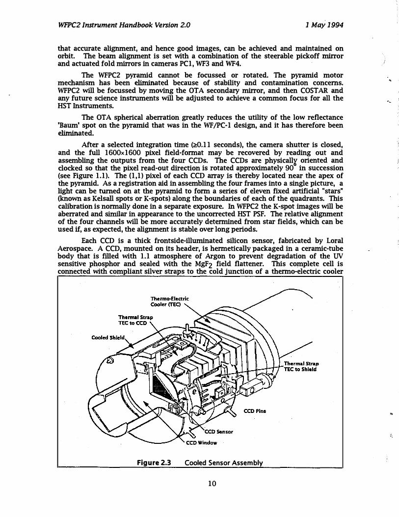
Each CCD is a thick frontside-illuminated silicon sensor, fabricated by Loral Aerospace. A CCD, mounted on its header, is hermetically packaged in a ceramic-tube body that is filled with 1.1 atmosphere of Argon to prevent degradation of the UV sensitive phosphor and sealed with the MgF2 field flattener. This complete cell is connected with compliant silver straps to the cold junction of a thermo-electric cooler
Figure 2.3 Cooled Sensor Assembly
10
..

('
WfPC2 Instru ment Handbook Version 2.0 1 May 1994
(TEC). The hot junction of the TEC is connected to the radial bay external radiator by an Ammonia heat pipe. This sensor-head assembly is shown in Figure 2.3. During operation, each TEC cools its sensor package to suppress dark current in the CCD.
2.4. QUANTUM EFFICIENCY The WFPC2 provides a useful sensitivity from 1150A to 11000A in each detector.
The overall spectral response of the system is shown in Figure 2.4 (not including filter transmissions). The CUlVes represent the probability that a photon that enters the 204m diameter HST aperture at a field position near the center of one of the detectors will pass all the aperture obscurations, reflect from all the mirrors, and eventually be detected as an electron in the CCD. The throughput of the system combined with each filter is tabulated in Table 6.1 and also shown in the Appendix.
Thermal vacuum testing and on orbit results have essentially confirmed the throughput estimates in version 1.0 of this handbook for wavelengths longward of 3500A. A comparison of these throughput values with those available from the WF/PC-1 IDT SV report indicates that WFPC-2 is a factor of a little under 2 less sensitive than WF /PC -1 (because its chips are not thinned). For a given background level, on an isolated point source WFPC2 would be about 2 times more sensitive than WF /pC-1 because of the improved PSF. However, WFPC2 has an intrinsically much lower equivalent background level (by a factor of 2 when sky limited and by a factor of 10-16 when read noise limited), so the overall gain in sensitivity is between about 3 and 8.
Below 2000A the data from the thermal vacuum testing were unclear. A Xe
..... 10 ::J c...
L en ::J o �
L I-
E � 5 CIl >. (j)
Figure 2.4
-- On orbit measurement·
........... Pre-launch prediction
2000 4000 6000 8000 10000 Wavelength (Angstroms)
WFPC2 + OTA System Throughput. The measurements made on orbit are better than the pre-launch estimates, and are used consistently elsewhere in this handbook. However they are preliminary, and result from observations on a small subset of the filters and standards.
11

WfPC2 Instru ment Handbook Version 2.0 1 May 1994
lamp at 1470A was used to get an absolute efficiency measurement with the camera compared to a standard diode. The result was a factor of 2 below the predicted cmves presented in this handbook version 1.0 based on component level tests. The results of the on-orbit testing have confirmed this result. It is now believed that the discrepancy is caused by the WFPC mirror reflectivities each having being in error by about 1096.
The visible and red sensitivity of the WFPC2 is a property of the silicon from which the CCDs are fabricated. To achieve good ultraviolet response each CCD is coated with a thin film of lumogen, a phosphor. Lumogen converts photons with wavelengths <4800A into visible photons with wavelengths between 5100A and 5800A. The CCD detects these visible photons with good sensitivity. Beyond 4800A, the lumogen becomes transparent and acts to some degree as an anti-reflection coating. Thus, the full wavelength response is determined by the MgF2 field flattener cutoff on the shortwavelength end, and the silicon band-gap in the infrared at 1 .1 eV (-1 1 OOOA).
With the WFPC2 CCD sensors, images may be obtained in any spectral region defined by the chosen filter with high photometric quality, wide dynamic range, and excellent spatial resolution. The bright end of the dynamic range is limited by the 0.1 1 seconds minimum exposure time, and by the saturation level of the selected analog to digital converter, which is roughly 53000 or 27000e- per pixel. The maximum signal-tonoise ratio corresponding to a fully exposed pixel will be about 230. The faint end of the dynamic range is limited by photon noise, instrument read noise and, for the wide-band visible and infra-red filters, the sky background.
Table 2.2 gives characteristic values of the expected dynamic range in visual magnitudes for point sources. The minimum brightness is given for an integrated SIN ratio of 3, and the maximum corresponds to full range (selected as 53000e-). The quoted values assume an effective bandwidth of 1000A at about 5700A (the F569W filter). The Planets, and many other resolved sources, are observable in this filter with short exposures even if their integrated brightness exceeds the 8.5 magnitude limit.
Configuration
Wide Field Wide Field Planetary Planetary
Exposure (seconds) Min. V Magnitude 0.11 8.83
3000. 19.92 0.11 8.46
3000. 19.55
Max. V. Magnitude
17.84 27.99 17.54 27.96
Table 2.2 WFPC2 Dynamic Range in a Single Exposure
2.5. SHUTTER
The shutter is a two-blade mechanism used to control the duration of the exposure. A listing of the possible exposure times is contained in Table 2.3. These are the only exposure times which can be commanded. Current policy is to round down non-valid exposure times to the next valid value. An exposure time of less than 0.1 1 seconds will therefore only result in a bias frame being taken.
Some exposures should be split into two (CR-SPLIT) in order to allow cosmic ray events to be removed in post-processing. By default, exposures of more than 10 minutes are CR-SPLIT. If an exposure is CR-SPLIT then the exposure time is halved (unless the user specifies a different fraction), and then rounded down. Note that some exposure times in the table do not correspond to commandable values when halved. In preparing a proposal that is to be CR-SPLIT, the simplest procedure to use in order to be sure of a given exposure time is to enter double a legal value.
For the shortest exposure times, it is possible to reconstruct the actual time of flight of the shutter blades. Encoder disks, attached to the shutter blade arms, are timed by means of a photo-transistor. The maximum error is 5 milliseconds. The
12
Wfl'C2 Instru ment Handbook Version 2.0 1 May 1994
necessary information is contained in the WFPC2 engineering data stream. However, this information is not in the processed science header.
When obtaining very short exposures, diffraction effects from the edges of the shutter blades affect the point spread function. Especially when using short exposures to obtain point spread functions in support of long exposure observations, it is advisable to use exposure times greater than 0.2s (see the WF/pC-I IDT OV/SV Report, Chapter 9 for further discussion in the spherically aberrated case).
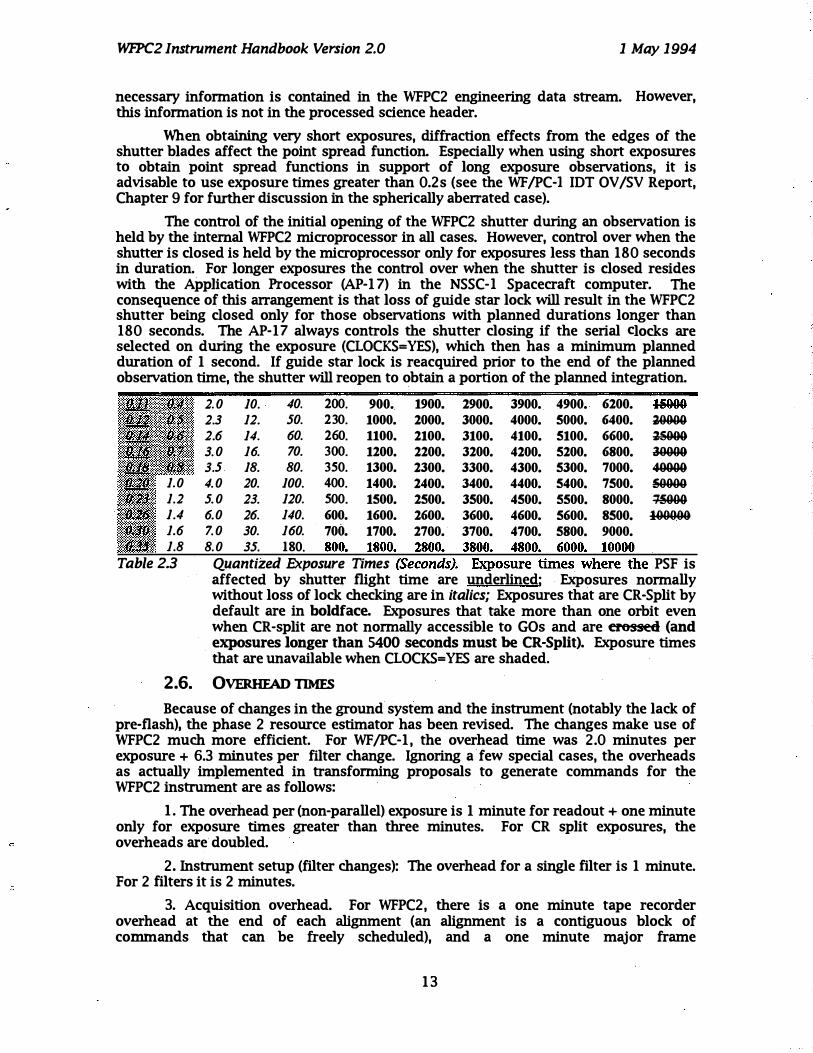
The control of the initial opening of the WFPC2 shutter during an observation is held by the internal WFPC2 microprocessor in all cases. However, control over when the shutter is closed is held by the microprocessor only for exp9sures less than 180 seconds in duration. For longer exposures the control over when the shutter is closed resides with the Application Processor (AP-1 7) in the NSSC-l Spacecraft computer. The consequence of this arrangement is that loss of guide star lock will result in the WFPC2 shutter being closed only for those observations with planned durations longer than 180 seconds. The AP-17 always controls the shutter closing if the serial clocks are selected on during the exposure (CLOCKS=YES), which then has a minimum planned duration of 1 second. If guide star lock is reacquired prior to the end of the planned observation time, the shutter will reopen to obtain a portion of the planned integration.
2. 0 10. 40. 200. 900. 1900. 2900. 3900. 4900. 6200. tsOOO 2.3 12. 50. 230. 1000. 2000. 3000. 4000. 5000. 6400. � 2.6 14. 60. 260. 1100. 2100. 3100. 4100. 5100. 6600. � 3. 0 16. 70. 300. 1200. 2200. 3200. 4200. 5200. 6800. 30000 3.5 18. 80. 350. 1300. 2300. 3300. 4300. 5300. 7000. 40000
1.0 4. 0 20. 100. 400. 1400. 2400. 3400. 4400. 5400. 7500. � 1.2 5. 0 23. 120. 500. 1500. 2500. 3500. 4500. 5500. 8000. � 1.4 6.0 26. 140. 600. 1600. 2600. 3600. 4600. 5600. 8500. 100000 1.6 7. 0 30. 160. 700. 1700. 2700. 3700. 4700. 5800. 9000. 1.8 8. 0 35. 180.
Table 2.3 Quantized Exposure Times PSF is affected by shutter flight time are underlined; Exposures normally without loss of lock checking are in italics; Exposures that are CR-Split by default are in boldface. Exposures that take more than one orbit even when CR-split are not normally accessible to GOs and are el'6ssed (and exposures longer than 5400 seconds must be CR-Split). Exposure times that are unavailable when CLOCKS=YES are shaded.
2.6. OVERHEAD TIMES Because of changes in the ground system and the instrument (notably the lack of
pre-flash), the phase 2 resource estimator has been revised. The changes make use of WFPC2 much more efficient. For WF/PC-1, the overhead time was 2.0 minutes per exposure + 6.3 minutes per filter change. Ignoring a · few special cases, the overheads as actually implemented in transforming proposals to generate commands for the WFPC2 instrument are as follows:
1 . The overhead per (non-parallel) exposure is 1 minute for readout + one minute only for exposure times greater than three minutes. For CR split exposures, the overheads are doubled.
2. Instrument setup (filter changes): The overhead for a single filter is 1 minute. For 2 filters it is 2 minutes.
3. Acquisition overhead. For WFPC2, there is a one minute tape recorder overhead at the end of each alignment (an alignment is a contiguous block of commands that can be freely scheduled), and a one minute major frame
1 3
WfPC2 Instru ment Handbook Version 2.0 1 May 1994
synchronization overhead. These two minutes are usually absorbed into the 12 minute overhead associated with guide star acquisitions and into the 6 minute· overhead associated with reacquisitions (generally each alignment has a seperate acquisition).
This information is provided for completeness and background. Guidelines in the Phase I proposal instru ctions and RPSS should be followed to develop Phase I and II proposals respectively.
It is not possible to schedule exposures in different filters less than 3 minutes apart. Commands to the WFPC2 are processed at spacecraft "major frame" intervals of one minute. A filter wheel may be returned to its "clear" position and another filter selected in one minute. An exposure takes a minimum. of one minute, and a readout of the CCDs takes one minute. There is no overhead time advantage in reading out a subset of the CCDs except when the WFPC2 readout occurs in parallel with the operation of a second instrument (where 2 minutes may be required to readout all 4 CCDs). Preflash overhead is eliminated because preflash is not necessary in WFPC2 to avoid deferred charge. The RPSS Resource Estimator should be used in developing Phase 2 proposals.
2.7. CCD ORIENTATION AND READOUT
The relation between the rows and columns for the four CCDs is shown in Figure 1.1. Note that each CCD is similarly sequenced, so that their axes are defined by a 90° rotation from the adjacent CCD. If an image were taken of the same field with each of the CCDs and then displayed with rows in the "X" direction and columns in the "Y" direction, each successive display would appear rotated by 90° from its predecessor.
The aberrated image of the pyramid edge is 40±14 pixels from the edge of the format along the two edges of each CCD which butt against the fields of view of neighboring CCDs. Figure 1.1 illustrates the projected orientation of the WFPC2 CCDs onto the sky. Because the beam is aberrated at the pyramid, there is a vignetted area at the inner edge of each field with a width of 4 arcseconds. The vignetted light ends up focussed in the corresponding position in the adjacent channel (with complementary vignetting). The inner edges of the field projected onto the CCDs are given in Table 2.4.
Camera Start Vignetted Field Contiguous field
PCI X>O and Y>8 X>44 and Y>S2 WF2 X>26 and Y>6 X>46 and Y>26 WF3 X>lO and Y>27 X>30 and Y>47 WF4 X>23 and Y>24 X>43 and Y>44
Start Unvignetted Field
X>88 and Y>96 X>66 and Y>46 X>SO and Y>67 X>63 and Y>64
Table 2.4 Inner Field Edges. The CCD �y (Column,Row) numbers given are uncertain at the 1 pixel level.
The WFPC2 has two readout formats, namely full single pixel resolution (FULL Mode), and 2x2 pixel summation (AREA Mode - obtained by specifying the optional parameter SUM=2x2 as described in the Proposal Instru ctions). Each line of science data is started with two words of engineering data, followed by 800 (FULL) or 400 (AREA) 16-bit positive numbers as read from the CCDs (with 12 significant bits). In FULL Mode the CCD pixels are followed by 11 "bias" words ("overclocked" pixels), making a total of 813 words per line for 800 lines. In AREA Mode, there are 14 bias words giving a total of 416 words per line for 400 lines. Either pixel format may be used to read out the WFC or Pc. These outputs are reformatted into the science image and extracted engineering data files during processing in the HST ground system prior to delivery to the observer.
The advantage of the AREA Mode (2x2) on-chip pixel summation is that readout noise is maintained at 7 electrons rms for the summed (i.e., larger) pixels. This pixel
14

WfPC2 Instrument Handbook Version 2.0 1 May 1994
summation is useful for some photometric observations of extended sources particularly in the UV. Cosmic ray removal is more difficult in AREA Mode.
The readout direction along the columns of each CCD is indicated by the small arrows near the center of each camera field in Figure 1.1. Columns and rows are parallel and orthogonal to the arrow, respectively. Each CCD is read out from the corner nearest the center of the diagram, with column (pixel) and row (line) numbers increasing from the diagram center. In a saturated exposure, blooming will occur almost exclusively along the columns because of the MPP operating mode of the CCDs. Diffraction spikes caused by the Optical Telescope Assembly and by the internal Cassegrain optics of the WFPC2 are at 45° to the edges of the CCDs. The default pointing position when all 4 CCDs are used is on WF3, approximately 10 arcseconds along each axis from the origin.
Observations which require only the field of view of a single CCD are best made with the target placed near the center of a single CCD rather than near the center of the 4 CCD mosaic. This will result in a marginally better point spread function, and avoid photometric, astrometric and cosmetic problems in the vicinity of the target caused by the overlap of the cameras.
While for such observations, only the field of view of a single CCD detector is actually required, the default operational mode is to read out all four CCDs. In the case of WF/pC-I, this policy resulted in serendipitous discoveries, and the recovery of useful observations in the case of small pointing or coordinate errors.
On the other hand any combination of 1, 2 or 3 CCDs may be read out in' numerical order (as specified in the Proposal Instructions). This partial readout capability is not generally available to GOs although it can be used if data volume constraints mandate it, after discussion with the WFPC2 instrument scientists. It does not result in a decrease in the readout overhead time but does conserve limited space on the HST on-board science tape recorder. The capacity of this tape recorder is slightly over 7 full (4 CCD) WFPC2 observations and 18 single CCD WFPC2 observations on a single side (of two). Switching sides of the tape recorder without a pause will result in the loss of part of a single CCD readout. Since an interval of about 30 minutes must normally be allowed for the tape recorder to be copied to the ground, readout of only a subset of the WFPC2 CCDs can be advantageous when many frames need to be obtained in rapid succession.
Multiple exposures may be obtained with or without spacecraft repointing between them followed by a readout with the restriction that the WFPC2 will be read out at least once per orbit.
15
WfPC2 Instru ment Handbook Version 2.0
3. OPTICAL FI L TERS
A set of 48 filters are included in WFPC2, with the following features:
1 May 1994
1 . It approximately replicates the WF/PC-I "UBVRI" photometry series.
2 . The broad-band filter series is extended into the far UV.
3. There is a new Stromgren series.
4. A Wood's fIlter is included for far-UV imaging without a red leak.
5. There is a 196 bandpass linear ramp filter series covering 3700-9800A.
6. The narrow-band series is more uniformly specifIed and better calibrated.
The filters are mounted in the Selectable Optical Filter Assembly (SOFA) between the shutter and the reflecting pyramid. The SOFA contains 1 2 filter wheels, each of which has 4 filters and a clear "home" position. A listing of all simple optical elements in the SOFA mechanism and the location of each element (by wheel number 1-12, and position 1-4) is given in Table 3.1. Wheel number 1 is located closest to the shutter. The categories of simple filters (F) are long-pass (LP), wide (W), medi� (M), and narrow (N). Most of these filters are either flat single substrates or sandwiches.
The filter complement includes two solar blind Wood's filters F160AW and FI60BW. F160BW will be used in all science observations because the other filter has some large pinholes that lead to significant redleak. .
In addition to the above complement of broad and narrowband filters WFPC2 features a set of three specialized quadrant (quad or Q) filters in which each quadrant corresponds to a facet of the pyramid, and therefore to a distinct camera relay. There is one quad containing four narrowband, redshifted [On] filters with central wavelengths from 3763-3986A, one quad with four polarizing elements (POL) with polarization angles, 0, 45, 90 and 135 degrees, and one quad with four methane (CH4) band filters with central wavelengths from 5433-8929A. The polarizer quad filter, can be crossed with any other filter over the wavelength range from 2800A to 8000A, with the exception of the Methane Quad and Redshifted [On] Quad which share the same wheel. The SOFA also contains four linearly variable narrowband ramp (FR) filters (in the twelfth wheel - closest to the focus). The quad and ramp filters are listed in Table 3.2
In Tables 3.1 and 3.2, each of the Type "A" filters is equivalent to inserting 5nun of quartz in terms of optical path length, with compensation for wavelength such that focus is maintained on the CCDs. A confIguration with no filters in the beam results in out-of-focus images and will not generally be used. With the exception of the quad polarizer and blocking (Type "B") filters, all filters are designed to be used alone. Type "B" filters introduce no focus shift, so they can be used in combination with any type "A:" filter. All combinations where the number of type "A" filters is not unity will result in out-of-focus images. The image blur resulting from two or zero type "A" filters at visible wavelengths is equivalent to 2.3 nun defocus in the F/24 beam, which corresponds to 1/5 wave rms of defocus at 6328A, and a geometrical image blur of 0.34 arcseconds. While this is a large defocus, the images are still of very high quality compared for example to seeing limited images. Some such combinations may be ScientifIcally attractive. For example, the Wood's filter may be crossed with another UV filter to provide a solar blind passband (although the effIciency will be low).
16

WfPC2 Instrument Handbook Version 2.0 1 May 1994
Name Type Wheel! Notes In r Ar Peak Peak Slot WF/PC-1 ? (A) (A) T (%) A. (A)
F122M A 1 4 H Ly alpha · Red Leak Y 1256 184.9 13.8 1247 F130LP B 2 1 CaFl Blocker (zero focus) N 3838 5568.2 94.7 4331 FI60AW A 1 3 Woods A • redleak from pinholes N 1471 466.5 19.0 1436 FI60BW A 1 2 Woods B N 1471 466.5 19.0 1436 F165LP B 2 2 Suprasil Blocker (zero focus) N 4357 5532.0 95.4 5788 F170W A 8 1 N 1675 469.5 26.2 1667 F185W A 8 2 N 1906 302.9 23.7 1849 Fl18W A 8 3 Interstellar Feature N 2136 354.5 22.2 2091 Fl55W A 8 4 N 2557 408.0 17.0 2483 F300W A 9 4 Wide U N 2925 727.8 47.9 2760 F336W A 3 1 WFPC2 U Y 3327 370.7 70.4 3447 F343N A 5 1 Ne V N 3430 24.8 19.7 3433 F375N A 5 2 [011] 3727 RS Y 3737 26.7 17.2 3736 F380W A 9 1 N 3934 694.7 65.0 3979 F390N A 5 3 CN N 3889 45.3 36.9 3885 F410M A 3 2 Stromgren nu N 4089 146.9 72.8 4098 F437N A 5 4 [0111] Y 4369 25.2 49.6 4368 F439W A 4 4 WFPC2 B Y 4292 ·464.4 71.3 4176 F450W A 10 4 Wide B N 4445 925.0 91.1 5061 F467M A 3 3 Stromgren b N 4682 171.4 80.0 4728 F469N A 6 1 He n y 4695 24.9 56.9 4699 F487N A 6 2 H beta y 4865 25.8 63.0 4863 F502N A 6 3 [0111] Y 5012 26.9 57.9 5009 F547M A 3 4 Stromgren y (but wider) Y 5454 486.6 86.6 5361 F555W A 9 2 WFPC2 V Y 5252 1222.5 94.9 5150 F569W A 4 2 F555W generally preferred Y 5554 965.7 92.0 5313 F588N A 6 4 He I & Na I (NaD) y 5892 49.1 92.1 5895 F606W A 10 2 Wide V Y 5843 1578.7 98.3 6187 F622W A 9 3 Y 6157 935.4 96.2 6034 F631N A 7 1 [01] Y 6283 30.6 90.2 6281 F656N A 7 2 H-alpha Y 6562 21.9 86.2 6561 F658N A 7 3 [NlI] Y 6590 28.5 83.3 6592 F673N A 7 4 [SII] Y 6733 47.2 82.1 6733 F675W A 4 3 WFPC2 R Y 6735 889.4 98.6 6796 F702W A 10 3 Wide R Y 6997 1480.7 99.0 6539 F785LP A 2 3 F814W generally preferred Y 9367 2094.8 98.3 9960 F791W A 4 F814W generally preferred Y 8006 1304.2 99.4 8081 F814W A 10 WFPC2 1 Y 8269 1758.0 98.7 8386 F850LP A 2 4 Y 9703 1669.5 94.2 10026 F953N A 1 1 [Sill] N 9542 54.5 90.7 9530 FI042M A 1 1 2 Y 10443 610.9 95.2 10139
Table 3.1 WfPC2 Simple ('F) Filter Set. The effective wavelength. width and transmission quoted are defined in Chapter 6. but do not include the system (OTA+WfPC2) response.
The mean wavelength r is similar to that defined in Schneider, Gunn and Hoessel (Ap. J. 264, 337). The width is the FWHM of a Gaussian filter with the same second moment and is reasonably close to the FWHM. The values tabulated here do not include the CCD DQE or the transmission of the OTA or WFPC2 optics (as given in Figure 2.4).
" . In Chapter 6 the corresponding quantities are given including the effect of the other optical elements and the CCD DQE.
1 7

MPC2 Instru ment Handbook Version 2.0 1 May 1994
Name Type Wheell Notes In t At Peak Peak Slot WF/PC-1 ? (A) (A) T (%) A. (A)
FQUVN·A A 1 1 3 Redshifted [011] 375 N 3766 73.4 24.0 3769 FQUVN·B A 1 1 3 Rcdshifted [Oll] 383 N 3831 $7.4 30.5 3827 FQUVN-C A 1 1 3 Rcdshifted [011] 391 N 3913 59.3 38.9 3908 FQUVN·D A 1 1 3 Redshifted [011] 399 N 3993 63.6 43.4 3990 FQCH4N·A A 1 1 4 CH4 543 N 5462 72.3 83.8 5442 FQCH4N·B A 1 1 4 CH4 619 N 6265 1$7.7 83.7 6202 FQCH4N-C A 1 1 4 CH4 727 N 7324 1 12.4 89.7 7279 FQCH4N·D A 1 1 4 CH4 892 N 8915 68.2 91.2 8930 POLQ..par B 1 1 1 0,45,90,135 N 5427 $797.6 90.8 10992 POLQ..per B 1 1 1 0,45,90,135 N 7922 66S3.4 89.7 10992 FR418N A 12 1 3700-4720 N W W/l00 -20-50 W FRS33N A 12 2 4720-6022 N W W/I00 -40·50 W FR680N A 12 3 6022·7683 N W W/I00 -60·80 W FR868N A 12 4 7683·9802 N W W/I00 -70·8S W
Table 3.2 MPC2 quad and ramp filters The quad polarizer is represented for both parallel and perpendicular polarization to its polarization direction, which is different in each quadrant.
Figure 3.1 summarizes the normalized transmission curves for the simple ("F") filters and narrowband quad filters. It does not include curves for the polarizing quad, or the linear ramp filters which are documented in Sections 3.1 and 3.3 respectively. Individual filter transmission curves are shown in the Appendix in Sections 8.1 (filters alone) and 8.2 (system response included). Figure 3.1 divides the filters into the following groups:
A. Long pass filters designed to be used in combination with another filter.
B. Wide bandpass filters with FWHM -2 596 of the central wavelength.
C. Approximations to the UBVRI sequence generally with wider bandpasses, designed for use on faint sources.
D. A photometric set of approximations to UBVRI passbands (see Harris et al. 1991, A.J. 101, 677). Note, however, that the WFPC2 UBVRI series is not the Johnson-Cousins photometric series, neither is it identical with the WF/PC-1 series. See Chapter 6 for detailed comparisons.
E. Medium bandpass filters with FWHM -1096 of the central wavelength, including an approximation to the Stromgren photometric series.
F. Narrow bandpass filters for isolating individual spectral lines or bands.
G. Redshifted [Om and CH4 narrow bandpass quad filters.
Note that the UV filters have some degree of "red leak", which is quantified in Chapter 6 where the system response is included.
A passband calibration is maintained in the calibration database system (CDBS). It has been updated following on orbit calibrations. However, the full filter set has not been calibrated yet, and some inconsistencies remain in the calibration. The information given here must therefore be regarded as approximate and preliminary. In particular, the ground based calibration of the narrowband filters' central wavelengths has not been corrected for temperature effects and is therefore accurate to about 2A. Because of this, it is not advisable to place narrow emission lines at the half power points of such filters and expect to predict the throughput to high accuracy. Either the standalone software package XCAL or SYNPHOT running under IRAF can be used to access these calibrations which are available on STEIS.
18

WfPC2 Instru ment Handbook Version 2.0
., ., 5
r��tr: ' � 1 000 2000 3000
z
2000 3000
4000 5000 6000 7000
Wavelength (Angstroms)
Wide Fi lters only
5000 6000 7000
Wovelength (Angstroms)
4000 5000 6000 7000
Wove length (Angstroms)
8000 9000
.................... 8000 9000
8000 9000
1 May 1994
1 0000 1 1 000
1 0000 1 1 000
1 0000 1 1 000
., ., � 1 00
r-____ �----��� __ ��W�FP�C�2�U�B-V-R�I�F·�llt�e-rs�o�n�ly�--__ --��--�� ____ � :; 80
i \ro• " .',- , -_. y: ,�.
II:: 60 ,.f' !\.. '-..., ! I \ 1l 40 ,1\,. .;... .J! i .... � 28 � ____ � ____ � ____ �J��,�\�� ____ �:_· _�_,�,·�� .. � __ �.�� ____ �� __ � ______ -J
� 1 000 o 2000 3000
z .,
4000 5000 6000 7000
Wavelength (Angstroms) 8000 9000 1 0000 1 1 000
.,
f '�I� : It n 7u\:l
t
e
,�� � : r 1 � 1 0
u
OO
�---
2
-
00
-
0
----3
-
0
�
0
-
0
----4
�
0
�
0
�
0
��
5
�
0
�
00
-----
60
�
0
-
0
----7
-
0
�
0
-
0
----
8
-
0
�
0
-
0
----
9
-
0
�
00
----
1
-
0
�
0
-
0
-
0
---
1
�
1 000
Z Wovelength (Angstroms) II en �
1 00
r-____ �--__ � __ �����nNrO-r-ro-w�Fnil�te7r-s�o-n+ly------�----�--�� ____ � ! �g ���;����;��;; f��a� ,::r.' ... ,; .. :i,I:.i .. , . �!�,.!i •••• ,� ••• , Ii 11 11 ::.:::::�::.:::: f!ii� i 28 � ____ � ___ F_�_§��� __ ������ ____ ��II�ID�H�=_::�_·;:_::_::_::_::�: ____ ����� ____ -J
(; 1 000 2000 3000 4000 5000 6000 7000 8000
Z Wavelength (Angstroms) 9000 1 0000 1 1 000
=:
f '�� ���� li�e �� :Qur], "nIYJ : 11 : � g
1 0
�
00
-----
2
�
00
-
0
----
3
�
0
�
0
-
0
--�
4
�
0
�
0
-
0
----
5
-
0
�
00
��-
60
�
0
�
0
�--7
-
0
�
0
-
O
ll---
8
-
0
�
O
-
0
----
9
w
O
�
00
----1
-
0
�
0
-
O
-
O
---
I
-J
l
000
Z Wavelength (Angstroms)
Figure 3.1 Summary of Normalized Filter Curves
19
WFPC2 Instru ment Handbook Version 2.0 1 May 1994
3.1. CHOICE OF BROAD BAND FILTERS
A number of different choices are possible on WFPC2 in order to approximate the Johnson Cousins system often used in ground based observing. These choices differ in throughput, wavelength fidelity, color transformability and cosmetics. The science program as a whole clearly benefits if a standard set for broad band photomeoy can be agreed upon by the community. This will allow theoretical isocbrones and other models to be published in the standard system, and allow ready comparison of the results from different observers. Furthermore although all filters will be calibrated photometrically and with flat fields, a core set must be chosen for monitoring the instrument both photometrically and in imaging performance. There is a substantial consensus between the accepted cycle 4 GO programs, the WFPC 1 and 2 science teams, and the Medium Deep Survey key project. In the case of the cool stars TAC panel for cycle 4, the accepted programs are mandated to use a standard system, unless the proposer is able to provide compelling scientific reasons for a different choice. AU GOs are therefore strongly encouraged to use F336W, F439W, F555W, F675W, and F814W as approximate equivalents to Johnson Cousins U, B, V, R, I passbands. These filters form the basis for the WFPC2 broad band photometric system. Note that the previous version of the WFPC2 handbook listed FS69W as a best choice for a V bandpass, and F791 W for the I bandbass. These choices are marginally better approximations to the Johnson Cousins passbands, but are not as efficient as the preferred filters. Also, the thermal vacuum results indicate that some dust is present on F791W, and this affects the flatfie�d. As will be seen from the figures in Chapter 6, the preferred set is accurately transformable with the exception of the U bandpass which is not particularly well simulated by any choice.
An edited summary of the cycle 4 TAC cool star panel recommendation is as follows:
"Cycle 4 will see the execution of several imaging programs which involve color-magnitude photometry of old stellar systems (globular clusters and dwarf galaxies). These individual programs are highly complementary to one another, and will have a major impact on our understanding of the chronology of the early Milky Way Galaxy and its satellites. The cumulative impact of these programs will be very much like that of a LargelKey Project in both size and scientific scope.
"Much of the scientific value of the combined programs will come after each is individually complete and when the color-magnitude data are directly compared, to produce discussions of the relative ages, metallicities, and other properties of the stellar systems concerned. In view of this, the Panel regards it as essential that the different observational groups should use the SAME FILTERS wherever feasible, and thus to remove any potential difficulties later in transforming between different photometriC systems. Most of the programs listed above intend to use the (V,/) band passes, but not all are requesting the same filters to define those bands.
" The Panel's opinion is that these filter choices should be MANDATORY. That is, all the programs must use the filters as listed above unless they can make a very strong scientific case to the contrary to the Director during the Phase 2 preparations. "
3.2. LINEAR. RAMP FILTERS
The linear ramp filters are designed for narrowband absorption and emission line imaging of moderately extended objects. Each filter is divided into four parallel strips where the central wavelength across each strip varies by approximately 6%. Each CCD pixel is, thus, mapped to a unique central wavelength with a FWHM band width of approximately 196 of the central wavelength. The ·maximum size ·of an object which can be imaged at a given wavelength is approximately 1 3 arcseconds and is determined by the width of the strips and the image size at the filter. The cumulative wavelength range of the four linear ramp filters is 3700 to 9802 A. Originally intended for a four WFC configuration, the linear ramp filters require partial rotation of the SOFA wheels to -18 and -33 degrees from their nominal positions, to recover 'wavelength regions which would fall on the PC camera or otherwise be lost. There will be vignetting at some wavelengths for these partial rotations.
20

WfPC2 Instrument Handbook Version 2.0 1 May 1994
3.2.1. Spectral Response
A JPL Interoffice Memorandum DM # 2031 (December 30, 1992) gives the results of a prediction scheme to locate and quantify the passbands of the four WFPC2 flight ramp filters, RF418n, RF533n, RF680n and RF866n. The results are summarized here.
Laboratory (room temperature) measurements of the passbands of the four ramp filters were made at 5 equally spaced intervals on each of the four ramp stripes on each filter for a total of 80 passband measurements. The laboratory measurements were made with a narrow beam and were then integrated over a "donut" area of the filter to simulate the beam profile at the ramp filter. The radius of the beam is 3.7nim, or 1 3 arcseconds. The integration was carried out by assuming the nominal linear shift in wavelength with position and that no significant changes in the passband shape occur across the beam. The integration makes the shape of the passband quite symmetric. The resulting curves can then be fitted to within a few percent with a Munson function:
T = 1'0 / {I + (1- a)x2 + a(1- b)x4 + ab(1 - c)x6 + abcxB}
where a, b and c are shape parameters, and Osa,b,c.s:l; To is the peak transmission of the passband, T=To at x=O; x is related to wavelength A. by x=(A.-Ac,)/H, T=T cl2 at x=1 (so His the half width at half maximum).
The parameters, (A.l)I T l)I H, a, b, c) were then fitted to polynomial functions of position Y (which starts at 0 inches at the lower wavelength edge of each strip) to predict the filter response for areas of the filters between the tested points. Good quadratic fits are in general available for all the parameters except for TO which requires a cubic. The results are given in Tables 3.3 through 3.6, which give the polynomial fit coefficients for the ramp filter parameters. The Table entries except for the first line are used as parameter=Ao+Aj Y+A2y2+A3y3. The short wavelength side of the filter is opposite for alternate ramps. The first line in each table gives Yposition as
-a.e -c o
'iii In 'E In C e ....
.:Je. C Q) a..
1 00
80
60
40
20
, / ..... , /\ ,.<'\ / ' �I /\ I 1 ; \ / r, I I I I I I I I I I I I I I I I I I , I I \�\" � , f\ 1 \
f \
II I I I ,I '" . , '\I I f Y v I I I " I
1 \ I ' \ I
I \ I
I I
,
, / ., .,'
I \" ,. ,r,
,.,. ;' �
, ,.
o �� ____ �� ____ �� ____ �� ____ �� ____ �� ____ �� ____ ���
2000
Figure 3.2
4000 6000 Wavelength (A)
8000 1 0000
Ramp Filter Peak Transmission. The four line types correspond to the four different filters (each containing four ramps)
2 1

WR'C2 Instrument Handbook Version 2.0 1 May 1994
0.020 I I I
-
0.01 5 I- -
_ .':.,. - . _ . _ . .. - . - . ... .
0.005 f0-r-
" - . _ . ... . ...
-
-
O.OOO �� __ � __ ��I�� __ � __ ��J __ � __ � __ L-�I __ � __ ����
2000 4000 6000 BOOO Wavelength {A}
Figure 3.3 Ramp Filter Dimensionless Widths
1 0000
a function of A.. If the polynomial fit predicts a, b, or c < 0 or > 1 then the quantities are set to 0 or 1 respectively.
Use of these fits should be restricted to objects on the center of the ramp ±7.6 arcseconds or the beam will combine light from adjacent ramps. The fit should also not be used within 1 3 arcseconds of the end of the ramp. There is enough overlap between ramps that positions inside the measured positions will be used for complete wavelength coverage except at the extreme end of the lowest and highest wavelength ramp. Figure 3.2 shows the fit parameter To as a function of AO for all 16 ramp filter strips. Figure 3.3 shows 2H/Ao
22

WFPC2 Instrument Handbook Version 2.0
Quantity
Ramp I Position WavelenctJa
Peak tl'lUllllliuJon HalhwldCh at halrmas
a II c:
Ramp 2 Position WavelenctJa
Peak tl'lUllllliuJon HaJrwldCh at halrmu
a II c:
Ramp 3 Position WavelenctJa
Peak transmisllon HalrwldCh at hair mas
a II c:
Ramp 4 Position WavelenctJa
Peak tl'llJlSlllilslon HaJrwldCh at half'mas
a b c:
AO Al Al -29.38 .0089 .0000 3657.7 138.7 .6178 -.01667 .2188 .04138
21.95 -.8347 2.143 .2120 .002857 .002596 1.181 -.8138 .3535 .3301 -.3715 .3825 -26.46 .0073 .0000 3876.9 158.6 .5472 .1660 .2288 -.1080 21.50 3.315 -.7079 .1592 -.003687 -;0008497 .7938 .2355 -.09124 .9306 .01366 .007458 -21.77 .0046 .0000 4130.5 168.8 -.7389 .1352 .6200 -.5226 22.09 1.306 -.1181 .2300 .05586 -.03044 1.096 -.3 185 .1396 1.276 -1.279 .5721
-24.39 .0058 .0000 4371.3 185.8 .2913 .3189 .1287 -.01 160 25.62 1.01S . 1 161 .3123 -.2055 .09535 .9222 .1 167 -.04673 1.033 -.1356 .05660
1 May 1 994
A3
-.03489
.004005
.1529
-.001712
Table 3.3 Ramp Filter FR41 8N parameters Note that FR41 8N is the name of the optical element, but it is used as generic filter LRF together with a specified wavelength in a proposal.
Quantity AO Al Al A3 Ramp I Position -21.77 .0037 .0000
WavelenctJa 4677.7 177.3 -1.125 Peak tl'llllSllllsslon .5450 -.3612 .3623 -.1281
HaJrwldCh at half'mas 25.67 .3168 .8873 a -.009839 .4644 -.2039 b .31 5 1 1 .9473 -.4516 c: -.3379 2.788 -1.346
Ramp 2 Position -26.79 .0058 .0000 Wavelen .... 4948.4 199.2 .6484
Peak tl'llllSllllsslon .4546 .4188 -.5456 0.1548 HaJrwfdCh at halrmas 32.10 -1.204 3.171
a .1678 -.02726 .09521 b .9345 .1935 -.1224 c: .9571 .02919 -.009393
Ramp 3 Position -19.98 .0030 .0000 Wavelength 5257.3 217.9 -1.481
Peak tl'llllSllllsslon .4944 -.1714 .1890 -0.0631 HaJrwldCh at half'mas 34.03 5.078 -1.347
a .3851 -.06264 .003163 b .5605 .6642 -.2751 c: .9665 .05543 -.03654
Ramp 4 Position -23.27 .0038 .0000 Wavelen"" 5596.9 220.9 -.6938
Peak tl'llllSllllsslon .5058 -.2715 .3203 -.1230 HaJrwldth at half'mas 35.06 -2.856 2.382
a .06553 .2253 -.08275 b 1.043 -.1190 .02889 c: 1.162 -.4910 .2059
Table 3.4 Ramp Filter FR533N parameters
23

WfPC2 Instrument Handbook Version 2.0 1 May 1994
Quantity AO At A2 A3 Ramp t PoIItlon -22.�7 .0039 .0000
WavelenatJa �916.0 269.4 .3460 Peak tl'lUlSllllallon .1 198 1.00� -.401� -.00162
Halfwldth at half mu 4UO -�.873 4.038 a .1743 -.O�OSO .06481 .. .8320 .3326 -.18�8 e .9682 -.09110 .0�122
Ramp 2 PoIItion -24.16 .0041 .0000 , . WavelenatJa 6290.8 27�.6 .7184
Peak tnnsmbalon .7918 -.02034 .1086 -.OS94S HalCwldth at halfmu 39.48 2.120 .3703
a .OSS96 .3034 -.1333 .. 1.017 -.27026 .04�60 e .7244 .8326 -.SI07
Ramp 3 Position -22.66 .003� .0000 WavelenatJa 6673.� 301.6 .3321
Peak tl'lUlSmlsslon .9494 -1.008 1.161 -.3777 HalCwldth at halCmu 42.81 .8193 .4269
a .1038 .09020 -.02747 b .84lS .304S -.1930 e 1.017 -.1732 .07463
Ramp 4 Position -24.0� .0033 .0000 WavelenatJa 7141.9 289.3 -.2999
Peak tl'lUlSmlsslon .4823 .4479 -.07484 -.0�868 Halfwldth at halCmu: 44.72 .89�2 -.07�6
a .1612 -.01167 .013�S b .2708 1.077 -.47�7 e .9941 -.02694 .0168S
Table 3.5 Ramp Filter FR680N parameters
Quantity AO At A2 A3 Ramp 1 Position -26.76 .0040 .0000
Wavelength . 7���.� 320,4 1.906 Peak tl'lUlSmlsslon .7�24 -.3328 .4�43 -.1343
HalCwldth at halCmu: 49.32 1.742 .4914 a .29�8 -.3877 .246S b 1.321 -.91�6 .3666 e .3762 1.668 -.9499
Ramp 2 Position -21.73 .0026 .0000 Wavelength 8014.3 3�0.� -.7�00
Peak tl'lUlSmlsslon .8204 -.3368 .381� -.10�7 HalCwldth at halCmu: �4.17 U79 .2196
a .0�832 .7�2S -.362� b .4�82 .8433 -.43�0 e .6422 .3247 -.1�93
Ramp 3 Position -23.16 .0028 .0000 Wavelength 8�10.7 37�.6 .3706
Peak tl'lUlSmlsslon .�817 -.1920 .4�17 -.1627 HalCwldth at halCmu �S.19 -.74S9 1.433
a .�422 -.2444 .03�4S b 1.420 -1.176 .4814 e .42�7 -.2�22 .1777
Ramp 4 Position -24.�4 .0029 .0000 WavelenatJa 9034.3 387.2 .8722
Peak tl'lUlSmlsslon .6241 .2403 -.1230 .02829 HalCwldth at halCmu: �9.69 2.167 -.1996
a .2376 -.01879 -.00864 b .9670 .024�6 -.00477 e .7829 .037�0 . 02393 ..
Table 3.6 Ramp Filter FR868N parameters
24

WfPC2 Instrument Handbook Version 2.0 1 May 1994
FR418N FR533N
- - - - - - - - - -.. - - - - .. - - - - -. 4442 4441 I I 4987 5075 1 1
1 i I I I I I I
I 1 I I
4572 -'- 4329 I 1 i 1 I 1 1 I I
1 1 1 1
4884 5166 1
4573 4325 4325 I 4325
1 r 1 I
1 I I I I I I
4713 4202 4170 I 3716 I
4875 5176 5176 1 5176
1 r 1 1
1 1 1 1 I 1 I
4770 5295 5371 1
5978 1
FR680N FR860N
6026 6803 - - - - 7 - - - - -1
1 i I 1 I I I 1
1 1 1 1 1 6205 6619 1
9248 9247 - - - - 1 - - - - -
1
i 1 I
1 1 1 1 1
1 1 1 1 1
9453 8954 1 6220 I 6603 6603 I 6603
1 1 1 I 1 I I I I I I
6402 6417 7176 I 7274
9476 I 8931 8413 7916
1 r 1 1 1 1 1 1 1 1 1
9785 8691 8690 1 7659
Figure 3.4 Ramp Filter Wavelength Mapping.
In Figure 3.4 we show the correspondence between central wavelength and location in the focal plane for the nominal filter positions. Rotated ramp filter positions are not shown here but are available seperately in a WFPC2 Instrument Science Report. The selection of filter and aperture for the linear ramp filters is transparent to the user who is required only to specify the lIDear ramp filter name LRF and a central wavelength for the observation. Each central wavelength is assigned to a unique filter and CCD location. Following thermal vacuum testing of · WFPC2 a revised table of linear ramp filter wavelengths has been compiled and is shown in Table 3.7. The vignetted regions close to the pyramid edges are avoided. The wavelength range 3700 - 9800A covered by the linear ramp filters is not continuous. Table 3.8 lists gaps in the wavelength coverage. It is also important to note that at the ends of each wavelength range on the filters, extended objects will be vignetted (Table 3.7 includes the pixel coordinates for the start and end wavelengths for each range). The boundaries of each strip correspond to the edge of the CCD at one end and the edge of the field near the pyramid at the other. While alternative locations for some wavelengths may be possible, they are not supported in order to ensure that a given central wavelength always corresponds to a single location within the unvignetted field of view. This scheme also permits standardization of the calibration requirements for these filters.
25

WfPC2 Instrument Handbook Version 2.0 1 May 1 994
Start {A� End {A� Filter CCO Pos X1 Pos Y1 Pos X2 Pos Y2 3716 381 5 FR4 1 8N WF4-FIX 796.6 736 67 736 3818 3877 FR41 8N33 WF3-FIX 683.3 432.9 446.4 68 3886 3921 FR41 8N33 WF2-FIX 70 425.2 286.9 284.7 3921 401 9 FR41 8N1 8 WF2-FIX 672.9 1 99.8 71 395.4 4025 4055 FR41 8N1 8 WF3-FIX 392.3 70 652.2 233.3 4057 4 1 70 FR4 1 8N WF4-FIX 67.8 3 1 2 797.7 3 1 2 4202 4325 FR4 1 8N WF3-FIX 238 796.6 238 76.2 4329 4441 FR4 1 8N WF2-FIX 70.9 253 763 253 4442 4572 FR41 8N WF2-FIX 785.2 729 65 729 4573 471 3 FR4 1 8N WF3-FIX 714 73 71 4 799 4770 4875 FR533N WF3-FIX 714 799.8 7 1 4 72 4884 4987 FR533N WF2-FIX 70 729 787.3 729 5039 5074 FR533N1 8 WF2-FIX 772.9 696 572 758 5075 5166 FR533N WF2-FIX 61 5.9 279 66.4 279 5176 5295 FR533N WF3-FIX 264 76.9 264 795.5 5371 5499 FR533N WF4-FIX 795.2 292 72.4 292 5542 5673 FR533N1 8 WF2-FIX 70 4 1 7 773.6 1 88.1 5673 5680 FR533N33 WF2-FIX 692.7 550.6 725.8 529.1 5704 5750 FR533N33 WF2-FIX 286.2 280.4 73.1 41 8.8 5763 5842 FR533N33 WF3-FIX 443 70 681 436 5847 5978 FR533N WF4-FIX 71 740 797 740 6026 6205 FR680N WF2-FIX 784.8 739 70 . 739 6220 6402 FR680N WF3-FIX 724 73 724 799.8 641 7 6603 FR680N WF3-FIX 248 798.5 248 74 661 9 6803 FR680N WF2-FIX 71 263 787.5 263 6804 6861 FR680N33 · WF2-FIX 498 668 323.7 780.7 6862 6946 FR680N1 8 WF2-FIX 354 3 1 6 69 409 6964 71 76 FR680N1 8 WF3-FIX 41 3.4 75 647.4 795 71 76 721 8 FR680N WF4-FIX 650 300 799.3 300 7274 7468 FR680N WF4-FIX 796.3 750 71 750 7476 7560 FR680N1 8 WF4-FIX 352.3 44.7 71 1 36 7561 7592 FR680N33 WF3-FIX 496.2 1 70.6 433.1 73.4 761 1 7658 FR680N33 WF2-FIX 69.2 409.4 279 273 7659 7916 FR868N WF4-FIX 796 758 69 758 7946 8032 FR868N1 8 WF4-FIX 301 70 70 1 45 8042 831 8 FR868N1 8 WF2-FIX 781 89 70 393.5 8341 8403 FR868N1 8 WF3-FIX 387 70 436 223 841 3 8690 FR868N WF4-FIX 70 324 798.6 324 8691 8931 FR868N WF3-FIX 224 656 224 70 8954 9247 FR868N WF2-FIX 69 239 784 239 9248 9453 FR868N WF2-FIX 552 729 68 729 9476 9785 FR868N WF3-FIX 714 68 714 798.8
Table 3.7 Aperture Locations and Wavelengths for Ramp Filters.
26

WR'C2 Instrument Handbook Version 2.0
Start End Gap 381 5 381 8 3 3877 3886 9 3921 3921 0 401 9 4025 6 4055 4057 2 4170 4202 32 4325 4329 4 4441 4442 1 4572 4573 1 471 3 4770 57
Start End Gap 4875 4884 9 4987 5039 52 5074 5075 1 5166 5176 1 0 5295 5371 76 5499 5542 43 5680 5704 24 5750 5763 1 3 5842 5847 5 5978 6026 48
Start End Gap 6205 6220 1 5 6402 641 7 1 5 6603 661 9 1 6 6803 6804 1 6861 6862 1 6946 6964 1 8 7176 7176 0 721 8 7274 56 7468 7476 8 7560 7561 1
1 May 1994
Start End Gap 7592 761 1 1 9 7658 7659 1 7916 7946 30 8032 8042 1 0 831 8 8341 23 8403 841 3 1 0 8690 8691 1 8931 8954 23 9247 9248 1 9453 9476 23
Table 3.8 Unavailable Wavelengths for Ramp Filters.
3.3. REDSHIF lED [011] QUAD FILTERS
The redshifted [011] quad fIlter was designed to map onto a four faceted WFC configuration. A partial SOFA wheel rotation of -33 degrees is required to move filter quadrant 1 (3763A) into WF2 and WF3, with some vignetting of both camera fields. The fIlter projections associated with the redshifted [011] quad are shown in Figure 3.6.
The nominal and rotated fIlter wheel positions for the redshifted [011] quad fIlter are each associated with different filter names, in order to allow pipeline calibration and database retrievals to proceed smoothly. The specification for each filter name is summarized in Table 3.9 below. .
Filter FOV Aperture Mean Effective Name Location name Wavelength Width
FQUVN WF2 WF2 3986 1 14 FQUVN WF3 WF3 3916 90 FQUVN WF4 WF4 3839 90 FQUVN33 WF2 FQUVN33 3763 88
Comments
Nominal filter wheel position Nominal filter wheel position Nominal filter wheel position Filter rotated -33 degrees
Table 3.9 Redshifted [OIl] Quad Filter Elements
The required central wavelength is selected by fIlter name and aperture location. Filter element FQUVN (Filter Quad UltraViolet Narrow) has three possible apertures, each of which is nominally centered in one of the three WF channels and associated with a unique central wavelength, while the filter element FQUVN33 corresponds to a single central wavelength. In the proposal instructions a central wavelength is also requested, in addition to the fIlter name and aperture, to provide a consistency check. Aperture names are discussed further in Section 3.6.
3.4. POlARIZER QUAD FILTER
The polarizer quads were also designed to map onto a four faceted WFC configuration and, consequently, also require a partial filter rotation of -33 degrees to move the fIlter quadrant 1 (nominal polarization angle 135 degrees) into WFCs 2 and 3, with some vignetting of both camera fields. Several additional partial rotations have been added to allow observations with different polarization angles on the same CCD.
27
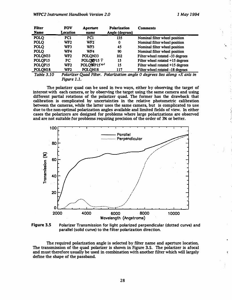
WR'C2 Instrument Handbook Version 2.0 1 May 1 994
Filter FOV Aperture Polarization Comments Name Location name Ansle �desreesl POLQ PCI PCI 135 Nominal filter wheel position POLQ WF2 WF2 0 Nominal filter wheel position POLQ WF3 WF3 45 Nominal filter wheel position POLQ WF4 WF4 90 Nominal filter wheel position POLQN33 WF2 POLQN33 102 Filter wheel rotated -33 degrees POLQPI5 PC POLQJ&15 '\l 15 Filter wheel rotated + 15 degrees POLQPI5 WF2 POLQ\W15\t-1 15 Filter wheel rotated + 15 degrees POLQNI8 WF2 POLQNI8 1 17 Filter wheel rotated -18 deGrees Table 3.10 Polarizer Quad Filter. Polarization angle 0 degrees lies along +X axis in
Figure 1.1.
The polarizer quad can be used in two ways, either by observing the target of interest with each camera, or by observing the target using the same camera and using different partial rotations of the polarizer quad. The former has the drawback that calibration is complicated by uncertainties in the relative photometric calibration between the cameras, while the latter uses the same camera, but is complicated to use due to the non-optimal polarization angles available and limited fields of view. In either cases the polarizers are designed for problems where large polarizations are observed and are not suitable for problems requiring precision of the order of 396 or better.
1 00
-� -c: 0 Or;; rD
'e rD c: E! I-
Figure 3.5
80
60
40
20
--- Parallel .................... Perpendicular
2000 4000 6000 · 8000 1 0000 Wavelength (Angstroms)
Polarizer Transmission for light polarized perpendicular (dotted curve) and parallel (solid curve) to the filter polarization direction.
The required polarization angle is selected by filter name and aperture location. The transmission of the quad polarizer is shown in Figure 3.S. The polarizer is afocal and must therefore usually be used in combination with another filter which will largely define the shape of the passband.
28
.�

WFPC2 Instrument Handbook Version 2.0
r
\...
1 35 0
. .
FQUVN33/POLQN33
POLQP1 5
1 May 1994
\/F"2 PCl
VF"3 \JF'4 ,
Figure 3.6 Redshifted [Om and Polarizer Quads. The schematics illustrate the field of view for unrotated and rotated polarizer filters. The greyscale flatfield images were obtained during thermal vacuum (PC field not to scale). The redshifted . FQUVN33 has the same field of view as POLQN33. An image of the filter POLQN1 5 1 ot yet available.
29
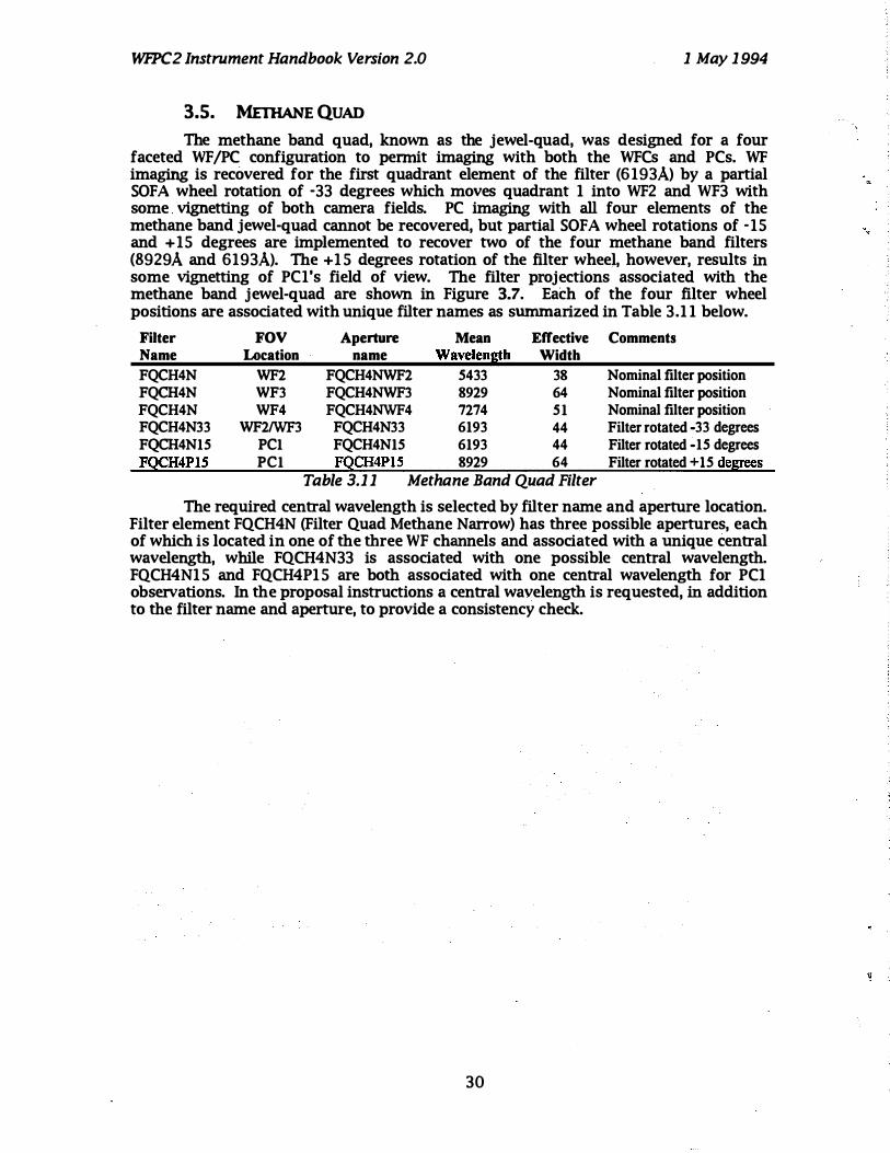
�2 Instrument Handbook Version 2.0 1 May 1 994
3.5. METHANE QUAD The methane band quad, known as the jewel-quad, was designed for a four
faceted WF /PC configuration to pennit imaging with both the WFCs and PCs. WF imaging is recovered for the first quadrant element of the filter (6193A) by a partial SOFA wheel rotation of -33 degrees which moves quadrant 1 into WF2 and WF3 with some vignetting of both camera fields. PC imaging with all four elements of the methane band jewel-quad cannot be recovered, but partial SOFA wheel rotations of -15 and +15 degrees are implemented to recover two of the four methane band filters (8929A and 6193A). The +1 5 degrees rotation of the filter wheel, however, results in some vignetting of PC1's field of view. The filter projections associated with the methane band jewel-quad are shown in Figure 3.7. Each of the four filter wheel positions are associated with unique filter names as summarized in Table 3.1 1 below.
Filter FOV Aperture Mean Effective Comments Name Location name Wavelength Width
FQCH4N WF2 FQCH4NWF2 5433 38 FQCH4N WF3 FQCH4NWF3 8929 64 FQCH4N WF4 FQCH4NWF4 7274 51 FQCH4N33 WF21WF3 FQCH4N33 6193 44 FQCH4N15 PC1 FQCH4N15 6193 44 FQCH4P15 PC1 FQCH4P15 8929 64
Table 3.1 1 Methane Band Quad Filter
Nominal filter position Nominal filter position Nominal filter position Filter rotated -33 degrees Filter rotated -15 degrees Filter rotated +15 degrees
The required central wavelength is selected by filter name and aperture location. Filter element FQCH4N (Filter Quad Methane Narrow) has three possible apertures, each of which is located in one of the three WF channels and associated with a unique central wavelength, while FQCH4N33 is associated with one possible central wavelength. FQCH4N1 5 and FQCH4P1 5 are both associated with one central wavelength for PC1 observations. In the proposal instructions a central wavelength is requested, in addition to the filter name and aperture, to provide a consistency check.
30

WFPC2 Instrument Handbook Version 2.0 1 May 1994
FQCH4N
FQCH4N33 -- --
FQCH4P15
FQCH4N15
Figure 3.7 Methane Quad Filter. The mapping to the. focal plane for nominal and rotated (-33, - 1 5 and +15 degrees) SOFA positions. The flatfield images on the right can be used to assess the unvignetted field. The PC1 field is not to scale in these images for clarity. Schematics illustrating the relative alignments are shown on the left.
3 1

Wfl'C2 Instrument Handbook Version 2.0 1 May 1994
3.6. WOOD'S Fn.TERS
WFPC2 features two solar-blind, or Wood's filters, for FUV « 2000A) imaging. It was shown by Wood in the 1930s (Physical Optics, 1949, R. W. Wood) that thin layers of alkali metals transmit FUV wavelengths while providing very efficient long wavelength blocking due to the plasma frequency of the free electrons. Wood's filters have been built for WFPC2 at JPL using thin (5000A) layers of sodium sandwiched between two MgF2 substrates. These sodium-based Wood's filters have a broad bandpass from 1200-2 100A with visible-light transmission lower than 10-8. The best conventional UV filters exhibit visible-light transmission of 10-3 to 10-4. Many astronomical objects emit 104 to 107 visible photons for every FUV photon. In such cases, a Wood's filter is essential for FUV imaging so that the visible light leak does not dominate the observation. The main problem experienced to date with Wood's filters is their long term stability. Sodium is a very reactive metal and attempts to passivate the sodium layer have met with limited success. It is possible that as the Wood's filters age pinholes will form which transmit visible light. This transmitted light will appear as an increase in the background level at the focal plane.
The Wood's filters can be used as a broadband filter or in combination with the CaF2 longpass filter to suppress geocoronal emission or crossed with one of the other UV filters to define a solar-blind UV photometric system. As discussed at the beginning of this Chapter, the image will be out of focus in the last case. WFPC2's Wood's filters are circular with a clear aperture of 41 Mm. Two similar Wood's filters are mounted in SOFA wheel 1 to provide some redundancy.
In the nominal filter wheel position PC1 has a clear field of view but, there is significant vignetting in all three WFCs. A partial filter wheel rotation of -1 5 degrees produces a larger field of view in WF3, although some vignetting remains. The options are illustrated in Figure 3.8. The imaging performance of the Wood's filters will be continually monitored for signs of "ageing such as pinhole visible light leaks. Additional partial rotations could be implemented in the future to pOSition an unaffected region of the filter into a WF or PC if necessary. The unvignetted filter projections associated with the two planned filter positions are shown schematically in Figure 3.8. Each filter
F160BW F160BN15 " Figure 3.8 Wood's Filters. Greyscale flat field images showing the field of
view available with the two Woods filter options Fl 60BW and F1 60BWN l S.
32

WfPC2 Instrument Handbook Version 2.0 1 May 1994
Filter FOV Aperture Mean Effective Comments Name Location Name Wavelength Width
Fl60BW PCI PCI 1600 900 Nominal filter position F160BNIS WF3 F160BNIS 1600 900 Filter rotated -IS degrees
Table 3.12 Wood's Filters
pOSition is associated with a unique name as summarized in Table 3.12 . .
The filter name required is selected on the basis of whether a PC or WF obseIVation is required.
In Thermal Vacuum testing, the two Wood's filters (F160AW and F160BW) performed well and were stable. F160AW however does show evidence for pinholes, which cause excessive redleak in some parts of its field. Therefore the preferred filter for far UV imaging with minimal redleak in WFPC2 is F160BW.
3.7. APERTURES
The WFPC2 camera configuration and filter set require a substantial number of new apertures. A summary of all possible aperture/filter combinations is given in Table 3.13.
Each camera has an associated 'optimum' aperture within its field of view (FOV) close to the field center of the CCD. The location for these apertures is close to the geometric center of each camera's field of view (after allowing for pyramid vignetting). . These pOSitions have been adjusted to reflect CCD performance following SMOV. The aperture designations are WF2, WF3, WF4 and PCI for the individual cameras and WFALL for the three WFC combination. WFALL is located close to the apex in WF3 (see Figure 1.1). ObseIVers are expected to place small or unresolved targets on these
. apertures. Note that normally all four CCDs are read out even if a specific CCD is selected with an aperture. This is discussed in Section 2.7.
In cases where the user does not want to use the current 'optimum' centers, a complimentary set of apertures has been implemented specifically for this purpose. These locations remain fixed and correspond roughly to the geometric center of each camera's field of view. They are designated WFl-FIX, WF2-FIX, WF3-FIX, PC1-FIX and WFALL-FIX. ObseIVers are expected to place extended targets on these apertures.
An additional set of aperture names have been defined for use with the WFPC2 filters which require partial rotations. The characteristics and uses of these filters are discussed earlier in this Chapter. In the nominal filter position, the three WFC segments of the [Om, Methane and Polarizer quad filters can be selected with an aperture for each camera corresponding to the optimum or geometric camera centers. The partially rotated quad filters, which generally fall into more than one camera, have been assigned apertures in the camera which provides the largest clear aperture. The pixel coordinates of these apertures will be reviewed on a regular basis to reflect changes in CCD and filter cosmetics. There are no analogous fixed apertures for the partially rotated filter configurations. The aperture name is generally the same as the (rotated) filter name. For the Wood's filters, the nominal filter position is used for the PCl FOV only, while the rotated filter position is used for WFC obseIVations. The linear ramp filters are unique because an aperture name is not required, since the ultimate location of the target will be determined from the central wavelength specified.
33

WFPC2 Instrument Handbook Version 2.0 1 May 1994
APERlURE CCO RLlER Loca tion Coord ina te s
XAO YAO pC , pC Optimu m c e nte r PC 1 420 424.5 WF2 WF2 O p timum c e nte r WF2 422.5 414 WF3 WF3 O p tim um c e nte r WF3 436l 424.5 WF4 WF4 O p timum c e nte r WF4 423 ' 421 �
WFALL WF3 O p timum loc a tio n nea r a p e x WF3 1 33 \ 1 49 PC 1-AX PC G e o metric c e nte r of FO V PC 1 420 \ 424.5 WF2-AX WF2 G e ometric c e nte r of FO V WF2 422.5 I 414 WF3-AX WF3 G e o m e tric c e nte r of FO V WF3 41 6.5-:.J 424.5 WF4-AX WF4 G e o m e tric c e nte r of FO V WF4 423 421 WFALL-AX WF3 Rxe d loc a tion n e a r a p e x WF3 1 33 1 49 FO UVN33 WF2 FO UVN33 O p timum in unvig nette d FO V WF2 292 520 PO LQN33 WF2 PO LQ N33 O ptim um in unvig nette d FO V WF2 292 520 PO LQ PP1 5 PC PO LQ P1 5 O ptim um in unvig netted FO V PC 1 200 680 PO LQWP 1 5 WF2 PO LQ P 1 5 O p timum in unvig nette d FO V WF2 500 260 PO LQ N 1 8 WF2 PO LQ N 1 8 O p tim um in unvig nette d FO V WF2 329 640 FO C H4NW2 WF2 FO C H4N O ptimum in unvig nette d FO V WF2 602 608 FO C H4NW3 WF3 FO C H4N O ptimum in unvig nett� d FO V WF3 602 608 FO C H4NW4 WF4 FO C H4N O ptim um in unvig nette d FO V WF4 640 386 FO C H4N33 WF2 FO C H4N33 O ptimum in unvig nette d FO V WF2 264 436 FO C H4N 1 5 PC FO C H4N 1 5 O ptim um in unvig nette d FO V PC 1 420 424.5 FO C H4P 1 5 PC FO C H4P15 O p timum in unvig nette d FO V PC 1 400 312 F1 60BN 1 5 WF3 F1 60BN 1 5 O ptimum in unvig nette d FO V WF3 41 6.5 424.5
Table 3.1 3 Aperture definitions. The coordinate system is (row, column) pixel numbers for the camera in use (see Figure 1 .1).
34

WR'C2 Instrument Handbook Version 2.0
4. CCO PERFORMANCE
4.1. INTRODUCTION
1 May 1994
It was originally intended that the WFPC2 CCDs would be Texas Instruments m) 800x800 CCDs, with Platinum bias gate electrodes to address the problem of quantum efficiency hysteresis (QEH). Subsequently, due to the limited availability of flight quality devices it was decided to design and fabricate a new CCD, based on the TI format, at Loral (formerly Ford Aerospace).
The WFPC2 CCDs are thick, front-side illuminated devices with a format of 800x800, 1 5x 1 5 pm. pixels. They are three-phase devices employing a recent CCD innovation, multi-pinned phase (MPP). MPP allows CCD exposure with the total inversion of all phases so that the Si-Si02 interface, at the surface of the CCD, can be pinned at the substrate potential, directing signal charge away from the Si-Si02 interface states towards the buried n-channel. Figure 4.1 shows a schematic which illustrates the principle of MPP (modified from Janesick et al. 1989). The frontside Si-Si02 interface significantly affects the performance of CCDs, so MPP operation yields many practical benefits including, reduced dark noise, optimal charge transfer efficiency (CTE), rapid removal of residual images, excellent pixel-to-pixel uniformity and improved radiation hardness. MPP technology has been demonstrated and characterized in both Loral Oanesick et al. 1989) and Tektronix devices (Woodgate et al. 1989). The CCD sensors for WFPC2 were manufactured by Loral in 1991 and processed and packaged for flight
Barrier __ ..... -....... Phase
o
-5
D
p
Collecting Phase
Distance (microns) •
p
6
·1 0 ______ � ______ L-____ � ______ � ______ L_ ____ � ______ �
A schematic showing the ideal potential profile through a frontside illuminated CCD whose front surface is inverted with multi-pinned phase (MPP). The CCD structure consists of a polysilicon gate, which forms part of the CCD's electrode structure, a surface layer of oxidized silicon (Si02) and the epitaxial layer which comprises p-doped silicon with an n-doped buried-channel for charge transfer. MPP pins the surface potential by populating the Si-Si02 interface with holes. The holes passivate the Si-Si02 interface states and create an electric field which directs signal charge away from the interface towards the buried n-channel.
Figure 4.1 MPP operating principle (schematic)
35

WFPC2 Instrument Handbook Version 2.0 1 May 1 994
at JPL
WF /pC -1 CCDs were thinned and 'back' illuminated, meaning that the active silicon layer is a free-standing membrane somewhat less than 10].llll thick, with photons impinging directly on the silicon layer without attenuation in the polysilicon gate structure built on the other ('front') side of the device. On the other hand, the Loral CCDs are illuminated from the 'front' surface, i.e. the light passes through the polysilicon gate structure overlying the 10].llll thick active silicon layer. Because the WFPC2 devices are frontside illuminated and supported by a bulk silicon substrate the CCD surface is flat, which is expected to reduce uncertainties in astrometric calibrations to about the 1/10 pixel level.
4.2. ceo CHARACTERISTICS
In this section the performance characteristics of the WFPC2 CCDs are reviewed and compared to the WF /pC -1 devices. In order to facilitate a rapid comparison a summary of device characteristics is presented in Table 4.1.
PARAMETER WFIPC-l WFPC2
Device Architecture
TI Thinned
Loral Thick
Dlumination Backside Frontside Format 800x800 800x800
Pixel size 15 JUIl2 15 JUIl2
UV Phosphor Coronene Lumogen Dark noise 0.03 e-/pixells(-8T') 0.016 e-/pixells(-7T') Read noise 13e- RMS 5e- RMS
Full Well Depth 40000 e- 90000 e-Gain 8e-IDN 7e-IDN or 14e-IDN
ADC range 12 bits (4096 DN) 12 bits (4096 DN) Full range (e1 -30000e- -53000e-
QE 6000A 50% 35% QE 2500A 12% 15%
WFC resolution 0.10 arcsec/pixel 0. 10 arcseclpixel PC resolution 0.043 arcsec/pixel 0.0455 arcsec/pixel
Table 4.1 Comparison Between WFJPC-I and WFPC2 CCDs
4.2.1. Quantum Efficiency
The Loral CCDs are thick, frontside illuminated devices and so their intrinsic QE is lower than thinned, backside-illuminated CCDs due to the absorption of some incident light by the polysilicon electrode structure on the frontside surface of the CCD. The phosphor coating, which converts UV light into the visual range, also produces an enhancement of DOE at visual wavelengths since it acts as an anti-reflection coating
The WF/PC-1 devices were overcoated with a coronene phosphor, which converts photons shortward of 3600A to longer wavelengths where the CCD DQE is high. The flat field appearance of the WF/PC-1 CCDs resulted from local variations in membrane thickness, and variations in thickness of residual inactive silicon and the electrostatic charge state at the back surface. A massive UV (2S00A) flood followed by maintenance of a continuous cold temperature was required to stabilize the backside charge state and OE of the WF /pC -1 CCDs. The QE instability was most pronounced in B band images.
In the WFPC2 devices, the front surface is overcoated with a lumogen phosphor, which serves as the primary detection medium for photons shortward of about 4800A,
36

WFPC2 Instrument Handbook Version 2.0 1 May 1 994
down-converting these to 5100-5800A. The QE of the Loral devices is stable without maintenance, hence the UV flood is unnecessary. Lumogen typically yields gains in DQE of 2-2.5 over the WF/pC-1 coronene phosphor for a given CCD. Its long wavelength cutoff (4800A) is -also better matched to a CCD's intrinsic sensitivity. The QE of the four flight WFPC2 CCDs is shown in Figure 4.2 and shows the uniform UV response of 10-1 596 and a peak optical QE of 4096.
50
40
-� 30 UJ o o
B 20 u
1 0
--- PC1
----···· .. ········· WF2
-----. WF3
- . - . - . - . _ . WF4
2000 4000 6000 8000 Wavelength (Angstroms)
Figure 4.2 WFPC2 Fl ight CCD DQE
4.2.2. Dynamic Range
1 0000
Linear full well capacity for these devices, clocked appropriately for the MPP mode, is approximately 70000e-/pixel. The full well capacity of the WF /pC -1 CCDs was about 40000e-, but signal level was set in practice by the system gain of 8e-ION and the ADC resolution of 1 2 bits giving ADC saturation at 30000e-. Flight qualified ADC with higher dynamic range (>12 bits) were not available so WFPC2 operates the two available ADCs at different gain factors. One channel has a gain of 14e-/DN, which significantly undersamples the CCD read noise (5e- RMS/pixel) and gives a digital full well of about 53000e-. The other channel has a gain of 7e-/DN, which is comparable to the CCD read noise and saturates at about 27000e-. The choice of gain factor will be detennmed by the scientific objective. The 7e-/DN channel is best suited to faint object and UV imaging, where the lower CCD read noise will be most effective. For example it should be used for UV imaging of planets or narrowband imaging of high redshift galaxies. The 14e-/DN channel has slightly higher effective read noise due to the quantization granularity but can be used for programs where a signal level in excess of 27000e- is required. Even when imaging faint sources, it may be sometimes be desirable to retain the high signal to noise information on brighter field stars as a PSF reference.
4.2.3. Bright Object Artefacts
Blooming up and down a CCD column occurs when more than about 100000e(the full well capacity) are collected in any pixel. When the pixel is full, the charge will
37

WfPC2 Instrument Handbook Version 2.0 1 May 1994
flow into the next pixels along the column, and so on. The orientation of the bloomed column(s) on the sky depends on the read-out direction of the particular CCO (see Figure 1 .1) and the roll angle of the spacecraft. This effect is visible in Figure 4.3 which shows a logarithmic stretch of the image resulting from 100 seconds exposure on a star of V magnitude 2 .6 through filter F502N in the Pc.
Extreme overexposure of the Loral CCOs is not believed to cause any permanent effects and therefore the WFPC2 does not have a bright object limit.
The WFPC2 CCOs can be operated in a non-standard mode during the integration phase of an exposure in order to limit the blooming to only those columns containing the bright sources. This is accomplished by operating the serial transfer register clocks during the integration (Using the optional parameter CLOCKS as specified in the Proposal Instructions). This will result in an enhanced dark current rate over much of the CCOs and is only necessary for overexposures expected to have signal levels of a few x 107 electrons within a single column. This mode is only possible for exposure times greater than 1 second.
Several other artefacts that are common in saturated stellar images are also obvious in in Figure 4.3. The Spider diffraction spikes caused by both the OTA spiders and internal WFPC2 spiders are at 45 degrees to the CCO columns in all cameras.
The halo around the stellar image is close to the diffraction limit in intensity and falls as the inverse cube of the angle subtended to the star.
Ouring readout of a badly overexposed image there is spurious charge detected by the readout electronics. This charge typically amounts to a level of 1.5 ON per saturated pixel with a lIe folding length of 400 pixels. The apparent brightness of the stellar halo is higher to the right of the saturated columns. This is particularly obvious at the bottom of the image in Figure 4.3 which is a region in the shadow of the pyramid edge.
Two filter ghosts caused by double (and quadruple) reflection inside the filter are visible below and to the right of the star. The position and brightness of these ghosts varies from filter to filter, typically being most obvious in interference filters. The comatic shape of the ghost is caused by the camera optics being effectively misaligned for the light path followed by the ghost. The relative position of these ghosts does not vary very much over the field.
The large ghost image expected to be caused by reflection off the CCO back to the filter and then back to the CCO is not seen. It was deliberately eliminated in the PC by tilting the CCO slightly.
An additional ghost is less obvious in this image can be seen closer to the . star than the filter ghost, and just above the bottom right spider diffraction spike. It is present in all filters and is caused by a reflection off the CCO, and a return reflection from the front of the MgF2 field flattener immediately in front of the CCO. The distance of this ghost from the star image varies linearly with the distance of the star image from a point near the center of the chip, because the field flattener is curved.
38
..

WfPC2 Instrument Handbook Version 2.0 1 May 1 994
Figure 4.3 Saturated Stellar Image
4.2.4. Residual Image Residual images in the WF /PC -1 CCDs occurred when the full well capacity was
exceeded, causing electrons to become trapped at the backside Si-Si02 surface interface. Trapped charge was slowly released over a period of time ranging from minutes to several hours, giving rise to residual images. A similar phenomenon, associated with the frontside Si-Si02 surface interface, is seen with frontside-illuminated CCDs. Inverted phase operation (MPP) allows holes to recombine with the trapped electrons at the frontside interface and so residual images dissipate very rapidly, on a timescale of minutes.
A second potential source of residual images, which occurs only in frontsideilluminated CCDs, is known as residual bulk image (RBI). Long wavelength photons can penetrate deeply enough to produce charge in the substrate. Most of this charge recombines rapidly (due to short carrier lifetimes) but some may diffuse into the epitaxial layer where it can become trapped in epitaxial interface states. Residual
39

WFPC2 Instrument Handbook Version 2.0 1 May 1994
images can occur as this charge is slowly released during an exposure. RBI is temperature sensitive since the bulk trapping time constants decrease with increasing temperature. The WFPC2 CCDs do exhibit RBI, but at -70°C trapped charge rapidly escapes so that residual images disappear within 1000 seconds. Driven by the WFPC2 electronics, the CCDs recover quickly from a large overexposures (100 times full well or more), showing no measurable residual images a half hour after the overexposure.
4.2.5. Quantum Efficiency Hysteresis
The problem of quantum efficiency hysteresis (QEH) due to backside charge accumulation has been reviewed in detail by Griffiths et ·al. (1989) and Janesick and Elliot (1991). QEH should not be present in the Loral CCDs because they are frontside illuminated and incorporate MPP operation, and this has been verified in component tests at ]pL. The absence of QEH means that the devices do not need to be UV-flooded and so decontamination procedures can be planned without the constraint of maintaining the UV-flood.
4.2.6. Flat Field
The flat field response is uniform within a few percent, with the exception of a manufacturing pattern defect which generates a 396 reduction in QE once every 34 rows. lbis pattern defect is identical in all CCDs, and also creates an astrometric offset of approximately 396 of the pixel height (0.003 arcsec in the WFCs) every 34 rows. More precisely, there was a 0.5JJlll overlap between adjacent 1024xO.5JJlll raster scans during the construction of the masks used to fabricate the chips. Photometry of point sources imaged onto these defects will be affected, and it will be better to correct flat fields for these rows for such applications. WFPC2 flat fields also include instrumental effects, such as vignetting and shadowing by dust particles.
The accuracy of flat fielding was one of the major limiting factors in the photometric calibration of scientific observations with WF /pC-I . The WFPC2 CCDs have intrinsically uniform flat field response since they are not thinned, so there are no large scale chip non-uniformities resulting from the thinning process. MPP operation also improves pixel-pixel uniformity because charge transfer is driven deep into the buried n-channel away from the influence of Si-Si02 interface states. The WFPC2 CCD flat fields show an overall pixel-to-pixel response having <296 non-unifOrmity. Figure 4.4 shows a portion of a WFPC2 CCD flat field obtained during quantum efficiency measurements at ]pL. The image illustrates the excellent pixel to pixel unifOrmity of the Loral devices. The 34 row defect is clearly visible, and its amplitude of 396 serves to calibrate the grey scale.
40
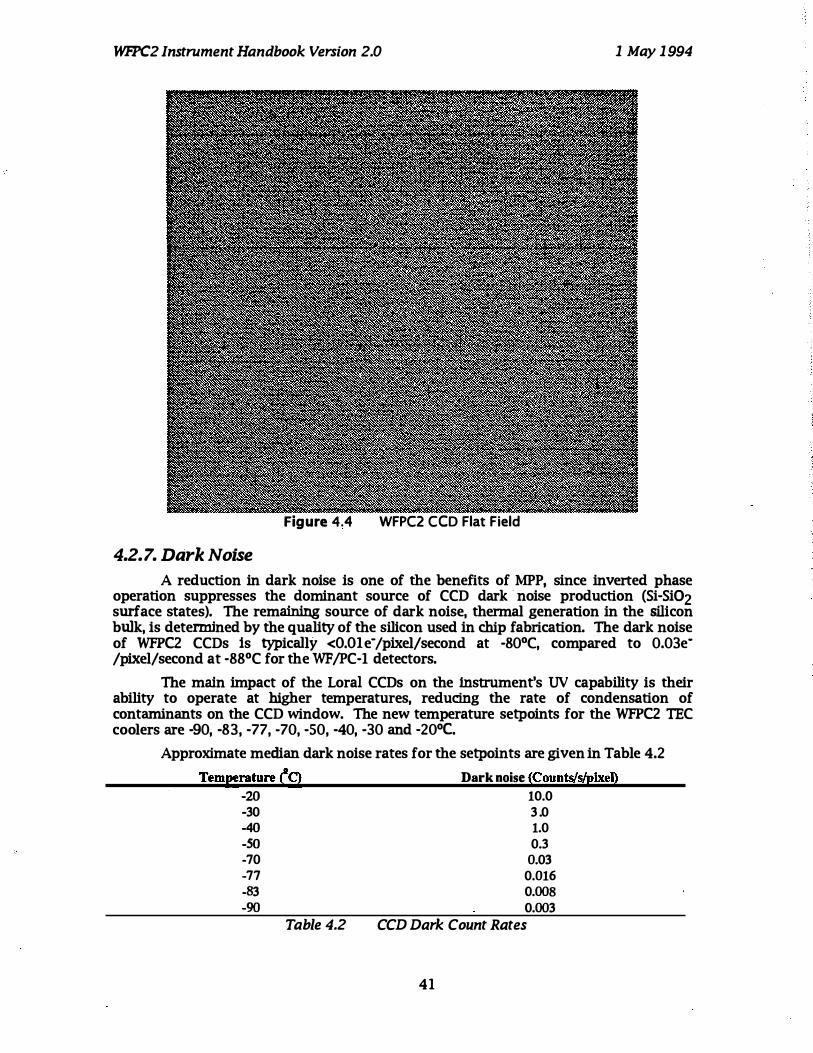
WFPC2 InstrumentHandbook Version 2.0
4.2.7. Dark Noise
Figure 4A WFPC2 CCD Flat Field
1 May 1 994
A reduction in dark noise is one of the benefits of MPP, since inverted phase operation suppresses the dominant source of CCD dark · noise production (Si-Si02 surface states). The remaining source of dark noise, thermal generation in the silicon bulk, is determined by the quality of the silicon used in chip fabrication. The dark noise of WFPC2 CCDs 1s typically <O.Ole-/pixel/second at -80°C, compared to 0.03e/pixel/second at -88°C for the WF/PC-1 detectors.
The main impact of the Lora! CCDs on the instrument's UV capability is their ability to operate at higher temperatures, reducing the rate of condensation of contaminants on the CCD window. The new temperature setpoints for the WFPC2 TEC coolers are -90, -83, -77, -70, -50, -40, -30 and -20°e.
Approximate median dark noise rates for the setpoints are given in Table 4.2
Temperature (9 -20 -30 -40 -SO -70 -77 -83 -90
Table 4.2
Dark noise (Counts/s/pixel)
10.0 3 .0 1.0
0.3 0.03
0.016 0.008
0.003
CCD Dark Count Rates
41
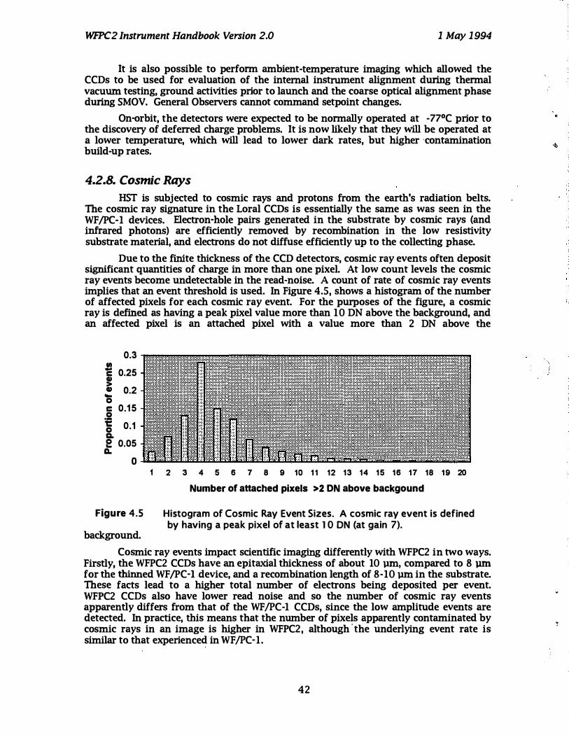
WfPC2 Instrument Handbook Version 2.0 1 May 1994
It is also possible to perfonn ambient-temperature imaging which allowed the CCDs to be used for evaluation of the internal instrument alignment during thennal vacuum testing, ground activities prior to launch and the coarse optical alignment phase during SMOV. General Observers cannot command setpoint changes.
On-orbit, the detectors were expected to be nonnally operated at -77°C prior to the discovery of deferred charge problems. It is now likely that they will be operated at a lower temperature, which will lead to lower dark rates, but higher contamination build-up rates.
4.2.8. Cosmic Rays
HST is subjected to cosmic rays and protons from the earth's radiation belts. The cosmic ray Signature in the Loral CCDs is essentially the same as was seen in the WF /pC -1 devices. Electron-hole pairs generated in the substrate by cosmic rays (and infrared photons) are efficiently removed by recombination in the low resistivity substrate material, and electrons do not diffuse efficiently up to the collecting phase.
Due to the finite thickness of the CCD detectors, cosmic ray events often deposit significant quantities of charge in more than one pixel. At low count levels the cosmic ray events become undetectable in the read-noise. A count of rate of cosmic ray events implies that an event threshold is used. In Figure 4.5, shows a histogram of the number of affected pixels for each cosmic ray event. For the purposes of the figure, a cosmic ray is defined as having a peak pixel value more than 10 DN above the background, and an affected pixel is an attached pixel with a value more than 2 DN above the
0.3
-E 0.25 ! '0
0.2
c 0.1 5 o i 0.1 a. e 0.05
D. o
Figure 4.5
background.
2 3 4 5 6 7 8 9 10 1 1 12 13 14 1 5 16 17 18 1 9 20 Number of attached pixels >2 ON above backgound
Histogram of Cosmic Ray Event Sizes. A cosmic ray event is defined by having a peak pixel of at least l O ON (at gain 7).
Cosmic ray events impact scientific imaging differently with WFPC2 in two ways. Firstly, the WFPC2 CCDs have an epitaxial thickness of about 10 pm, compared to 8 pm. for the thinned WF /pC-I . device, and a recombination length of 8-10 pm in the substrate. These facts lead to a higher total number of electrons being deposited per event. WFPC2 CCDs also have lower read noise and so the number of cosmic ray events apparently differs from that of the WF /PC -1 CCDs, since the low amplitude events are detected. In practice, this means that the number of pixels apparently contaminated by cosmic rays in an image is higher in WFPC2, although ' the underlying event rate is similar to that experienced in WF /PC-I.
42
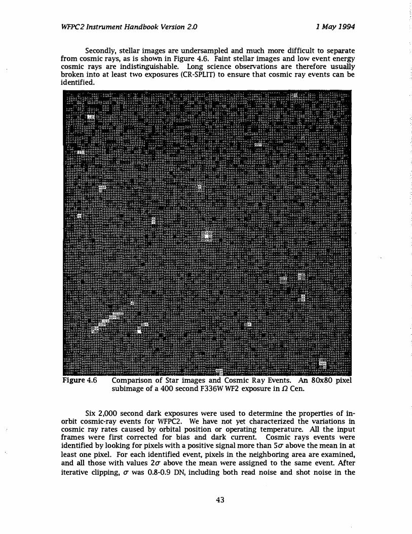
WFPC2 Instrument Handbook Version 2.0 1 May 1994
Secondly, stellar images are undersampled and much more difficult to separate from cosmic rays, as is shown in Figure 4.6. Faint stellar images and low event energy cosmic rays are indistinguishable. Long science observations are therefore usually broken into at least two exposures (CR-SPLIT) to ensure that cosmic ray events can be identified.
Figure 4.6 Comparison of Star images and Cosmic Ray Events. An 80x80 pixel subimage of a 400 second F336W WF2 exposure in [2 Cen.
Six 2,000 second dark exposures were used to determine the properties of inorbit cosmic-ray events for WFPC2. We have not yet characterized the variations in cosmic ray rates caused by orbital position or operating temperature. All the input frames were first corrected for bias and dark current. Cosmic rays events were identified by looking for pixels with a positive signal more than 50" above the mean in at least one pixel. For each identified event, pixels in the neighboring area are examined, and all those with values 20" above the mean were assigned to the same event. After iterative clipping, 0" was 0.8-0.9 DN, including both read noise and shot noise in the
43
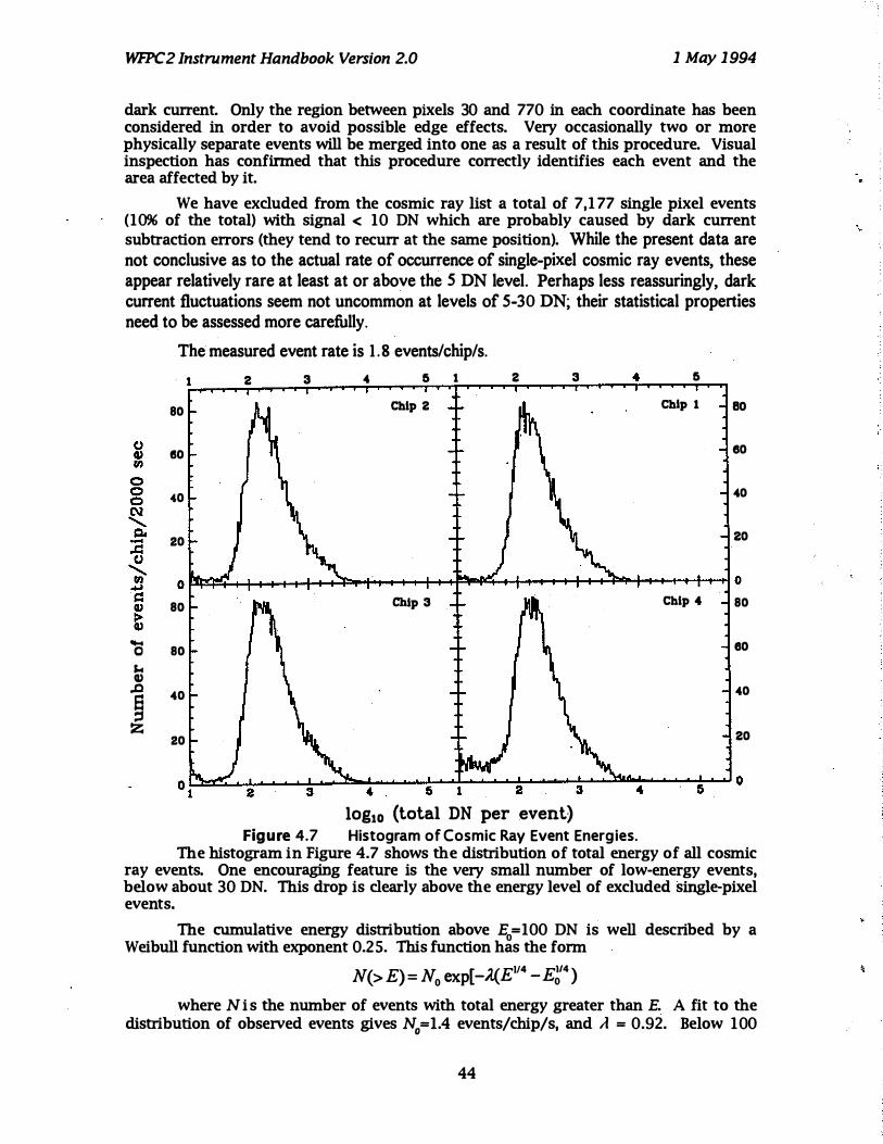
WfPC2 Instrument Handbook Version 2.0 1 May 1994
dark current. Only the region between pixels 30 and 770 in each coordinate has been considered in order to avoid possible edge effects. Very occasionally two or more physically separate events will be merged into one as a result of this procedure. Visual inspection has confirmed that this procedure correctly identifies each event and the area affected by it.
We have excluded from the cosmic ray list a total of 7,1 77 single pixel events (1096 of the total) with signal < 10 DN which are probably caused by dark current subtraction errors (they tend to recurr at the same position). While the present data are not conclusive as to the actual rate of occurrence of single-pixel cosmic ray events, these appear relatively rare at least at or above the 5 DN level. Perhaps less reassuringly, dark current fluctuations seem not uncommon at levels of 5-30 DN; their statistical properties need to be assessed more carefully.
-o ... Q)
.c § Z
The measured event rate is 1 .8 events/chip/so
1 2
80
eo
40
20
3 4 5 1
Chip 2
2 3 5
ChIp 1 80
80
40
20
o����++�������������++�����++�� O 80 ChIp 3 Chip " 80
80
40
20
80
40
20
���������--���������������6�� 0 2 3 " 5 1 2 3 "
IOglO (total DN per event) Figu re 4.7 Histogram of Cosmic Ray Event Energies.
The histogram in Figure 4.7 shows the distribution of total energy of all cosmic ray events. One encouraging feature is the very small number of low-energy events, below about 30 DN. This drop is clearly above the energy level of excluded single-pixel events.
The cumulative energy distribution above Eo=100 DN is well described by a Weibull function with exponent 0.25. This function has the form
N(> E) = No exp[-A.{EII4 _E�4 ) where N i s the number of events with total energy greater than E. A fit to the
distribution of observed events gives No=1.4 events/chip/s, and /I = 0.92. Below 100
44

WR'C2 Instrument Handbook Version 2.0 1 May 1 994
DN, the distribution flattens considerably, and the Weibull distribution should not be extrapolated. The total event rate below 100DN is about 0.4 eventS/chip/so
About 3.796 of the pixels will be affected by a cosmic ray in a 2000 s exposure. As cosmic rays can be expect to be randomly placed, one would expect that about 1 ,000 pixels per chip would be hit in both of two 2000s exposures, which would make cosmic ray removal impossible for those pixels. For a pair of 1000s exposures, about 220 pixels will be affected in both frames.
4.2.9. Radiation Damage
In low earth orbit (LEO) the CCDs are subject to radiation damage from the earth's radiation belts. The WFPC CCDs are shielded from energetic electrons, and about half the incident energetic protons. Long term radiation damage to the CCDs from high energy protons leads to an increase in dark count rate (mainly from the creation of hot pixels), baseline shifts in the CCD amplifiers and long term degradation of Charge Transfer Efficiency (CTE). There has not been a significant degradation in the amplifier baselines (although occasional small baseline shifts have been seen). There are no observed changes in CTE since launch. On the other hand; one of the major radiation damage mechanisms is the creation of new Si-Si02 interface states which cause increased dark current rates in affected pixels. In the MPP CCD these states immediately recombine with holes reducing the gradual increase in dark noise by factors of -2 5 compared to normal three-phase CCDs· (Woodgate et al. 1989, Janesick et al. 1989b). A long term dark frame program is monitoring. the increase in the number of hot pixels
4.2.10. Charge Transfer Efficiency
The WF/PC-l CCDs exhibited a low-level non-linearity, known as deferred charge, mainly due to charge traps in the CCD transfer gate, a design fault discussed by Janesick and Elliot (1991) and Griffiths, et al. (1989). In practice low signal levels « 250 e-) are effectively smeared over several pixels during transfer. Removing the problem required a preflash exposure (40e- pedestal) prior to the majority of science observations, increasing the read noise and adding to the overhead time associated with an exposure.
There are also significant deferred charge problems in the WFPC2 CCDs at the current operating temperature of -77 degrees. This has been observed to lead to a difference in count rate for a given point source of 1096 between the top and bottom rows on the chip (after flat-fielding). However, this problem is expected to be largely eliminated by operating the devices at -90 degrees. Successful proposers will be informed of the status of this problem in time for their phase 2 submissions.
4.2.1 1.Read Noise and Gain Settings
The CCDs and their associated signal chains have read-out noise levels (in the absence of signal shot noise or interference) of approximately 5e-. The WF/PC-l CCD read noise was effectively 1 5-20e-, since there were additional contributions above the nominal 1 3e- resulting from "missing codes" in the ADC and the preflash exposure.
The conversion factors from detected electrons (QE x number of incident photons) to data numbers (DN) are as tabulated in Table 4.3., as are read noise and linearity. Note that all calculations of sensitivity in this manual assume gains of 7 and 14 for two gain channels, choices very close to the meaured gains.
45
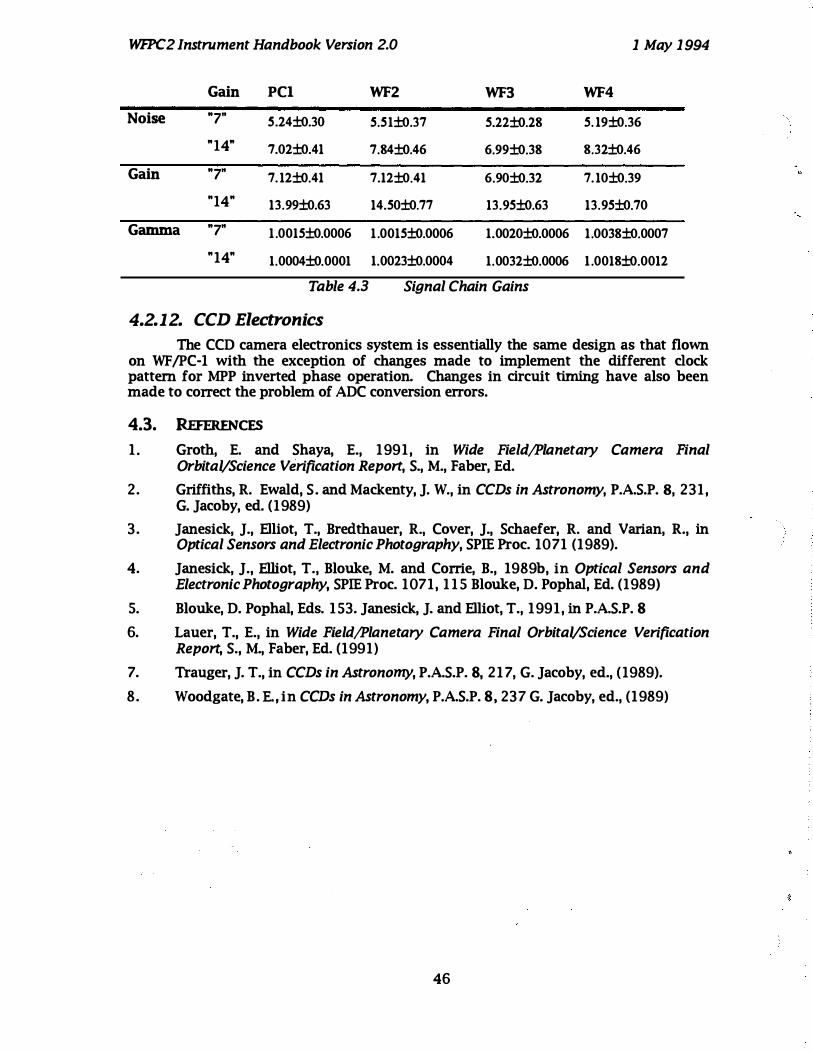
WfPC2 Instrument Handbook Version 2.0 1 May 1 994
Gain PCI WF2 WF3 WF4
Noise "7" S.24±o.30 S.Sl±o.37 S.22±o.28 S. 19±o.36
"14" 7.02±o.41 7.84±o.46 6.99±o.38 8.32±o.46
Gain "7" 7. 12±o.41 7.12±o.41 6.90±o.32 7. 10±o.39
"14" 13.99±o.63 14.S0±o.77 13.9S±o.63 13.9S±o.70
Gamma "7" l .OOlS±o.OOO6 l .OOlS±o.OOO6 l.OO20±o.OOO6 1.0038±o.OOO7
"14" l.OOO4±o.OOOl l.OO23±o.OOO4 l.OO32±o.OOO6 l .OO18±o.OO12
Table 4.3 Signal Chain Gains
4.2.12. CCD Electronics
The CCD camera electronics system is essentially the same design as that flown on WF /pC-1 with the exception of changes made to implement the different clock pattern for MPP inverted phase operation. Changes in circuit timing have also been made to correct the problem of ADC conversion errors.
4.3. REfERENCES
1 . Groth, E. and Shaya, E., 1991, in Wide Field/planetary Camera Final OrbitaVScience Verification Report, S., M., Faber, Ed.
2 . Griffiths, R. Ewald, S . and Mackenty, J. W., in CCDs in Astronomy, P.AS.P. 8, 231 , G. Jacoby, ed. (1989)
3 . Janesick, J., Elliot, T., Bredthauer, R., Cover, J., Schaefer, R. and Varian, R., in Optical Sensors and Electronic Photography, SPIE Proc. 1071 (1989).
4. Janesick, J., Elliot, T., Blouke, M. and Corrie, B., 1989b, in Optical Sensors and Electronic Photography, SPIE Proc. 1071, 1 1 5 Blouke, D. Pophal, Ed. (1989)
5. Blouke, D. Pophal, Eds. 1 53. Janesick, J. and Elliot, T., 1991, in P.AS.P. 8
6. Lauer, T., E., in Wide Field/planetary Camera Final OrbitaVScience Verification Report, S., M., Faber, Ed. (1991)
7. Trauger, J. T., in CCDs in Astronomy, P.AS.P. 8, 2 1 7, G. Jacoby, ed., ( 1989).
8 . Woodgate, B . E., in CCDs in Astronomy, P.AS.P. 8, 237 G. Jacoby, ed., (1989)
46
"

WfPC2 Instrument Handbook Version 2.0
s. POINT SPREAD FUNCTION
5.1. EFFEcrs OF OTA SPHERICAL ABERRATION
1 May 1 994
The OTA spherical aberration produces the Point Spread Function (PSF - the apparent surface brightness profile of a point source), that was observed by the WF/PC-1. Briefly, the fraction of the light within the central 0.1 arcsecond was reduced by a factor of about 5. The resulting PSF had "wings" which extended to large radii (several arcseconds), greatly reducing the contrast of the images and degrading the measurements of sources near bright objects or in crowded fields. Burrows et al. (1991, Ap. J. Lett. 369, L2 1) provide a more complete deScription of the aberrated HST PSF. Figure 5.1 shows the PSF in three cases. It shows the aberrated HST PSF, the WFPC2 PSF, and for comparison the PSF that would be obtained from a long integration if HST were installed at a ground based observatory with one arcsecond seeing. All the PSFs were computed at 4000A. The FWHM of the image both before and after the installation of WFPC2 is approximately proportional to wavelength but the WF /PC -1 core was approximately 5096 broader than the core that is obtained with WFPC2. Figure 5.2 shows the encircled energy (EE), the proportion of the total energy from a point source within a given radius of the image center, for the same three cases. The WFPC2 curve shown is the average of measurements taken with F336W and F439W. It can be seen that the core of the image in WFPC2 contains most of the light. At this wavelength, 6596 of the light is contained within a circle of radius 0.1 arcseconds. (WF/PC-1 had about 1 596). However, this proportion is considerably less than the optics deliver. The reason for this is discussed in the next section.
_____ WFPC2 PC (corrected)
_ _ _ _ _ _ _ _ WF /PC- 1 PC (aberrated)
_ . _ . _ . _ . _ . _ . _ . _ .PC ( 1 arcsec seeing) )( 1 0-2 ::3
� C .... oS -0
1 0-4 �
1 0-8 �_�_�_� __ �_�_�_��� __ �_�_�_� o
Figure 5.1
2 4 e
PSF Surface Brightness. The percentage of the total flux at 4000A falling on a PC pixel as a function of the distance from the peak of a star image.
47

Wf1'C2 Instrument Handbook Version 2.0 1 May 1 994
1 00 ���-'-T-r-r�==�::::::��_�._�. -�.�- .�- .�-�.�S.��.-�-���.-�. -�.�_ .�_�. _r-_�.���
... . - . /
80
� 60 �
� -
'0 M 40
20
. - ' /
� / / /
/ / , /
, / ,
//
,.' , / , / ,. / ,. /
/ // ,. /
,. / i /
i /
/"
.' //
! / ;' // WFPC2 PC (corrected)
i/ /.( / ! ________ .WF/PC-1 PC (aberrated)
/ ! I' ! / ! / / _ ._ . _ . _ . _ . _ . _ . _PC ( 1 arcsec seeing)
I ! I .'
I . ! I !
I .' ,
" , � '
2 Arcseconds 3 o
Figure 5.2 Encircled Energy. The percentage of the total flux at 4000A within a given radius of the image peak .
S.2. CCD PIxEL REsPONSE FUNCTION
From Thermal Vacuum testing, there was evidence that the images are not as sharp as expected despite the good wavefront quality. The decrease in sharpness corresponds to a loss in limiting magnitude of about 0.5 magnitudes in the WF cameras, and less decrease in the PC.
Further testing by covering a flight spare CCO with a 2 micron pinhole grid in an opaque metallic mask and illuminating with a flatfield source, showed that even when a pinhole was centered over a pixel only about 7096 of the light was detected in that pixel.
For practical Plll'Poses, the effect can be modelled as equivalent to about 30 milliarcseconds RMS gaussian jitter in the WFC and 14 milliarcseconds in the Pc. Alternatively, at least in the V band, it can be modelled by convolving a simulated image by the following kernel:
0.016
K= 0.080 0.015
0.067 0.635 0.078
0.016 0.080 0.015
One clue is the wavelength dependence of the observed sharpness: the results from the 2 micron pinhole grid test get worse at longer wavelengths. This may reflect the greater penetration into the silicon of low energy photons, which facilitates the diffusion of photoelectrons across the pixel boundaries defined by the frontside gate structure. There is also evidence for subpixel QE variations at the 1096 level. There is an implied dependence on pixel phase for stellar photometry. This has been seen at about the 196 level in on-orbit data. The very recent work of Jorden, Oeltom, and Oates (Greenwich Observatory Newsletter 9/93) has yielded quite similar results, and suggests that subpixel response must be taken into account when seeking to understand the behavior of all CCO detectors forming undersampled images.
48

Wf1'C2 Instrument Handbook Version 2.0 1 May 1994
5.3. MODEL PSFs
Considerable effort has gone into the modeling of the HST PSF, both in order to measure the optical abeITations in support of the WFPC2, COSTAR and advanced sdentific instruments and to provide PSFs for image deconvolution in the abeITated telescope. Such PSFs are noise free and do not require valuable HST observing time. Software to generate model PSFs for any filter and at any location within the field of view is available from the STScI. It can also be used to generate model PSFs for the WFPC2. The results are illustrated in Tables 5.1 and 5.2 for the PC1 and WF2 cameras respectively. A representative PSF is on the left in each panel. It meets the wavefront error budget, with the measured mix of focus, coma, astigmatism, and spherical aberration. It has been degraded by the pixel response function as discussed in the last section. On the right is the diffraction limited case for comparison. In each case the percentage of the total flux in a central 5x5 pixel region of a point source is displayed The peak of the star image can be at an arbitrary point relative to the boundaries of the CCD pixels. Two cases are shown: one where the star is approximately centered on a pixel, and one where it is approximately centered at a pixel comer. As a consequence of the under-sampling in the WFPC2, the limiting magnitude attainable in the background limit varies by about 0.5 magnitude, depending on the position of the source. This point is discussed in more detail in Chapter 6. .
Neither observed nor modeled PSFs will provide a perfect match to the PSF in actual sdence observations due to modeling uncertainties, the "jitter" in the HST pointing, and orbit to orbit variations in telescope focus ("breathing" - which seems to generally be limited to about 1/20 wave peak to peak). Jitter is not predictable but can be recovered to a reasonable extent for observations obtained in Fine Lock. In long exposures, up to about 10 milliarcseconds of apparent pointing drift may occur as a result of the breathing effects in the FGS.
49

WfPC2 Instrument Handbook Version 2.0 1 May 1 994
2000 A Peak near corner of PC pixel 1.3 2.6 2.4 2.1 0.1 0.2 0.5 0.4 0.3 0.1 3.3 7.4 7.2 2.5 0.7 0.5 14.3 20. 1 0.6 0.1 2.3 5.9 1 0.5 2.9 0.6 0.4 20. 1 30.8 0.6 0.2 1 .6 2.5 3.3 1 .8 0.6 0.3 0.6 0.6 0.3 0. 1 . "
0.5 0.9 0.7 0.7 0.5 0. 1 0.1 0.2 0. 1 0.2 Peak near center of pixel
0.7 1 . 3 1 .9 1 . 9 0.9 0.2 0.4 0.4 0.3 0.2 1 . 5 3.9 5.0 2.6 1 .2 0.4 0.9 6.8 0.5 0.2 2.1 5.6 14.9 5.1 1 .4 0.4 6.9 63. 1 4.2 0.4 1 .3 2.4 3.9 3.6 1 . 1 0.3 0.5 4.2 0.6 0.3 0.6 1 .4 1 .6 1 .2 0.6 0.2 0.2 0.4 0.3 0.2
4000 A Peak near corner of PC e.1xel 1 .0 2. 1 2.7 0.9 0.3 0.2 2.3 2.4 0.3 0. 1 3.2 9.1 1 0.2 3.0 0.5 2.3 12.8 1 5.5 2.8 0.2 2.2 9.6 1 2.3 3.6 0.6 2.4 1 5.5 1 9.4 3.1 0.2 0.6 2.5 3.2 1 .5 0.6 0.3 2.8 3.1 0.4 0. 1 0.2 0.4 0.5 0.6 0.3 0.1 0.2 0.2 0.1 0. 1
Peak near center of pixel 0.5 0.8 0.8 0.7 0.4 0. 1 0.2 0.5 0.2 0. 1 1 .2 4.3 6.3 4.0 0.7 0.2 4.4 5.4 3.8 0.2 1 . 0 6.5 22.7 6.0 0.9 0.5 5.4 48.7 4.2 0.3 0.5 2.7 5.4 4.0 0.9 0.2 3.8 4.2 3.6 0.2 0.3 0.4 0.6 0.9 0.5 0.1 0.2 0.3 0.2 0.1
6000 A Peak near corner of PC e.1xel 1 .9 2.4 3.0 2.2 0.4 2.0 2.3 2.0 2.1 0.2 3.2 8.7 9.7 2.8 0.6 2.3 1 0.4 12.7 2. 1 0.6 2.5 9.8 1 1 .2 3.2 0.7 1 .9 1 2.8 1 5.2 2.0 0.6 1 .4 2.6 3.0 2.3 0.6 2.0 2.0 2.0 2.3 0.2 0.3 0.5 0.7 0.6 0.2 0.2 0.5 0.6 0.2 0. 1
Peak near center of pixel 0.7 1 .4 1 .8 1 .7 0.5 0.3 1 . 9 1 .9 1 .6 0.3 2.0 3.3 6.3 3.2 1 . 3 1 . 8 2.3 5.8 2.2 1 .4 2.0 6.5 1 9.4 5.5 1 .5 1 . 9 5.8 3 1 . 3 4.0 1 . 8 1 . 1 2.6 5.0 3.4 1 .4 1 . 5 2. 1 4.0 2.4 1 .3 0.3 1 .1 1 .6 1 .4 0.6 0.2 1 . 3 1 . 8 1 . 3 0.2
BOOO A Peak near corner of PC eixel 1 .6 1 .8 2.0 1.8 1.1 1 .8 0.9 0.9 1 .5 1.1 2.0 8.6 9.3 2. 1 1 . 1 0.9 1 0.9 1 2.5 1 . 0 1 .4 1 . 9 9.4 1 0.2 2.4 1 . 1 0.9 12.5 14.0 1 . 1 1 . 5 1 . 3 2.0 2.2 1 . 8 1 . 1 1 . 5 1 .0 1 . 1 1 . 5 1 .3 0.8 1 . 1 1 . 3 1 . 1 0.5 1 . 1 1 .4 1 . 5 1 .3 0.2
Peak near center of pixel 1 .3 1 .3 1 .5 1 .7 1 . 3 1 .6 1 .6 1 . 0 1 .6 1 .4 1 .7 3.0 6.5 2.6 1 .5 1 .6 2.1 7.5 1 .7 1 .6 1 .6 6.6 14.8 5.6 1 .4 1 .0 7.5 22.2 5.7 1 .2 1 .2 2.6 5.3 2.5 1 .6 1 .6 1 .7 5.7 1 . 3 1 . 8 0.9 1 . 3 1 .4 1 .6 1 . 1 1 .4 1 .6 1 . 1 1 . 8 1 .2
Table 5.1 PC Point Spread Functions shown as percentages of the total flux in Q 5 by 5 pixel region On the left in each case is a model PSF with the observed wavefront errors and pixel response (unction. On the right is the diffraction limited case for comparison.
50

WfPC2 Instrument Handbook Version 2.0 1 May 1994
0.5 1.9 1 .5 1 0.2 1 .3 8.6 0.5 1 .9 0.2 0.4
0.2 0.5 0.4 2.1 0.6 6.3 0.3 2.1 0.3 0.5
0.8 2.4 2.4 1 4.7 1 .9 1 2.5 0.6 2.0 0.2 0.4
0.4 0.7 0.7 4.0 1 . 1 9.6 0.5 2.5 0.2 0.4
0.7 2.4 2.8 1 3.6 2.1 1 3.5 0.6 2.3 0.2 0.3
0.3 0.9 0.9 5.2 1 .0 8.6 0.5 2.9 0.2 0.5
0.9 2.7 3.3 12.2 2.5 1 2.5 0.7 3.3 0.2 0.4
0.3 0.9 1 . 1 5.3 1 .0 7.8 0.5 3.1 0.2 0.5
Table 5.2
2.3 1 4.8 23.6 3.5 0.3
0.7 6.6
30.0 7.8 0.9
2.3 1 5.8 1 9.3 2.9 0.3
0.9 8.3
33.2 7.5 0.7
2.5 1 5.3 1 7.9 3.2 0.4
1 .0 8.1
30.3 8.0 0.9
2.8 1 3.4 1 5.4 3.9 0.5
0.9 7.4
30.6 6.9 0.9
2000 A 0.9 3.4 4.7 1 .3 0.2
Peak near comer of WF §Ixel 0.3 0.4 .3 0.5 0.3 1 0.3 0.6 0.4 1 8.2 0.3 0.3 0.4 0.2 0.1 0.1
Peak near center of pixel 0.6 3.4
1 2.7 3.5 0.6
4000 A 0.7 3.1 3.3 1 .0 0.2
0.3 0.2 0.2 0.8 0.2 0.9 1 .8 0.2 1 .6 0.8 0.1 0.6 0.3 0.2 0.1
Peak near comer of WF §ixel 0.2 0.4 .5 0.5 0.5 1 4.0 0.4 0.5 20.2 0.2 0.2 0.6 0.1 0.1 0.1
Peak near center of pixel 0.6 0.3 0.3 0.3 3.5 0.6 0.2 0.9 8.6 0.9 0.4 6.0 2.4 0.5 0.2 0.7 0.5 0.2 0.2 0.2
6000 A Peak near comer of WF e,ixel 0.9 0.3 0.3 0.4 3.4 0.5 0.4 1 5.7 3.5 0.4 0.4 20.2 0.8 0.2 0.2 0.6 0.2 0.2 0.2 0.3
Peak near center of pixel 0.7 0.3 0.2 0.3 4.1 0.8 0.3 2.9 8.8 1 .1 0.3 6.2 3.0 0.5 0.3 1 .9 0.5 0.3 0.2 0.3
BOOO A Peak near comer of WF e,ixel 1 .1 0.3 0.1 1 .7 4.2 0.6 1 .7 1 4.2 3.8 0.5 1 .8 1 7.0 1 .1 0.3 0.2 2.4 0.2 0.1 0.2 0.1
Peak near center of pixel 0.8 0.3 0.1 0.2 4.5 0.9 0.2 4.2 7.5 1 .1 0.3 5.4 3.2 0.6 0.2 3.4 0.6 0.2 0.1 0.2
0.4 0.3 0.1 1 8.2 0.4 0.1 44.9 0.4 0.1 0.5 0.4 0.1 0.1 0.1 0.1
0.2 0.1 0.2 1 .6 0.6 0.1
86.0 1 .2 0.2 1 .2 0.8 0.1 0.2 0.2 0.2
0.5 0.2 0.1 20.2 0.6 0.1 32.2 0.6 0.1 0.6 0.4 0.2 0.1 0.2 0.2
0.4 0.2 0.2 6.0 0.7 0.2
68.6 3.0 0.3 3.0 0.7 0.1 0.3 0.2 0.3
0.4 0.2 0.2 20.2 0.5 0.3 27.5 0.7 0.2 0.7 0.2 0.2 0.2 0.3 0.2
0.3 0.3 0.2 6.2 1 .9 0.3
54.9 6.0 0.2 6.0 1 .5 0.3 0.2 0.3 0.2
1 .8 0.2 0.2 1 7.0 2.4 0.1 21 .4 2.8 0.1 2.8 0.2 0.2 0.1 0.2 0.1
0.3 0.2 0.1 5.4 3.4 0.1
5 1 .6 4.4 0.3 4.4 3.2 0.2 0.3 0.2 0.1
WF Point Spread Functions On the left in each case is a model PSF with the observed wavefront errors, and pixel response (unction. On the right is the diffraction limited case for comparison.
51

WFPC2 Instrument Handbook Version 2.0 1 May 1994
S.4. ABERRATION CORRECTION.
The strategy for correction of the HST aberration preserves the optical layout of WF/PC-I , but with steep corrective figure on the relay secondary mirrors and substantially tighter optical alignment tolerances. The optical correction implemented for WFPC2 recovers near-diffraction limited images over the entire CCD fields of view. The corrective optics enable essentially all of the scientific objectives of the original WF /PC to be met.
Camera
Design error Fabrication and alignment error
Alignment stability error Total wavefront error
Table 5.3
WFC (F/ll.9) 1J143 1J14.7 -1J25
1J12.6
PC(F/28 3) 1J50
1J.14.7 1J25
1J12.3 Wavefront Error Budget
Through a number of independent analyses, based on investigations of star images obtained on-orbit and the examination of fixtures used during the figuring of the primary mirror, the aberrations of the HST optics were accurately characterized. The surface of the primary mirror was figured to an incorrect conic constant: -1.0139±0.0005 rather than the -1.0023 design requirement, resulting in a large amount of spherical aberration. By design, WF /pC -1 created an image of the primary mirror near the surface of the relay cassegrain secondary mirror in each of its channels. This design was originally intended to minimize vignetting in the relay optics, but for WFPC2 the image (complete with the wavefront aberration) serves an additional purpose. The optical figure of the WFPC2 secondary mirrors was altered with the addition of a compensating 'error' in conic constant. By adopting a preScription within the error bars for the HST primary mirror, corrective secondary mirrors were made with sufficient accuracy that the residual spherical aberration in the WFPC2 wavefront is small compared to other terms in the WFPC2 optical wavefront budget. On the other hand, new and stringent alignment requirements were created by the steep optical figure on the corrective relay secondary mirrors. The primary mirror image must be accurately centered on the corrective mirror, and must have the correct magnification. Centering is the most demanding requirement. A failure to center accurately would create a new aberration in the form of coma. A misalignment of 796 of the pupil diameter introduces as much RMS wavefront error as was present in the form of spherical aberration prior to the introduction of corrective optics. The new requirements for alignment accuracy and stability lead to the introduction of a tip-tilt mechanism on the pickoff mirror to compensate for camera alignment uncertainties with respect to the OTA, and actuated fold mirrors which can compensate for internal misalignments. There was an additional term in the CElS specification of the overall instrument wavefront error budget for aligntnent stability. It is 1../25 RMS at 6328A, as shown in the Table 5.3.
The first two lines in the wavefront error budget are essentially identical to those for WF /PC-I. 'Design error' refers to the aberrations inherent in the design itself, which would be seen if the optics conformed perfectly to their specifications. All the optics were fabricated and integrated into the WFPC2 optical bench, and it was established on the basis of component tests, end-to-end optical interferometry, and through focus phase retrieval that the WFPC2 optical system performed within the stated tolerances for 'fabrication and alignment' in the laboratory environment. What remained was to demonstrate the stability of the optical alignment during launch vibrations, and in response to the thermal environment on-orbit. The 'stability' line anticipated these uncertainties, and has now been verified during early science operations.
52
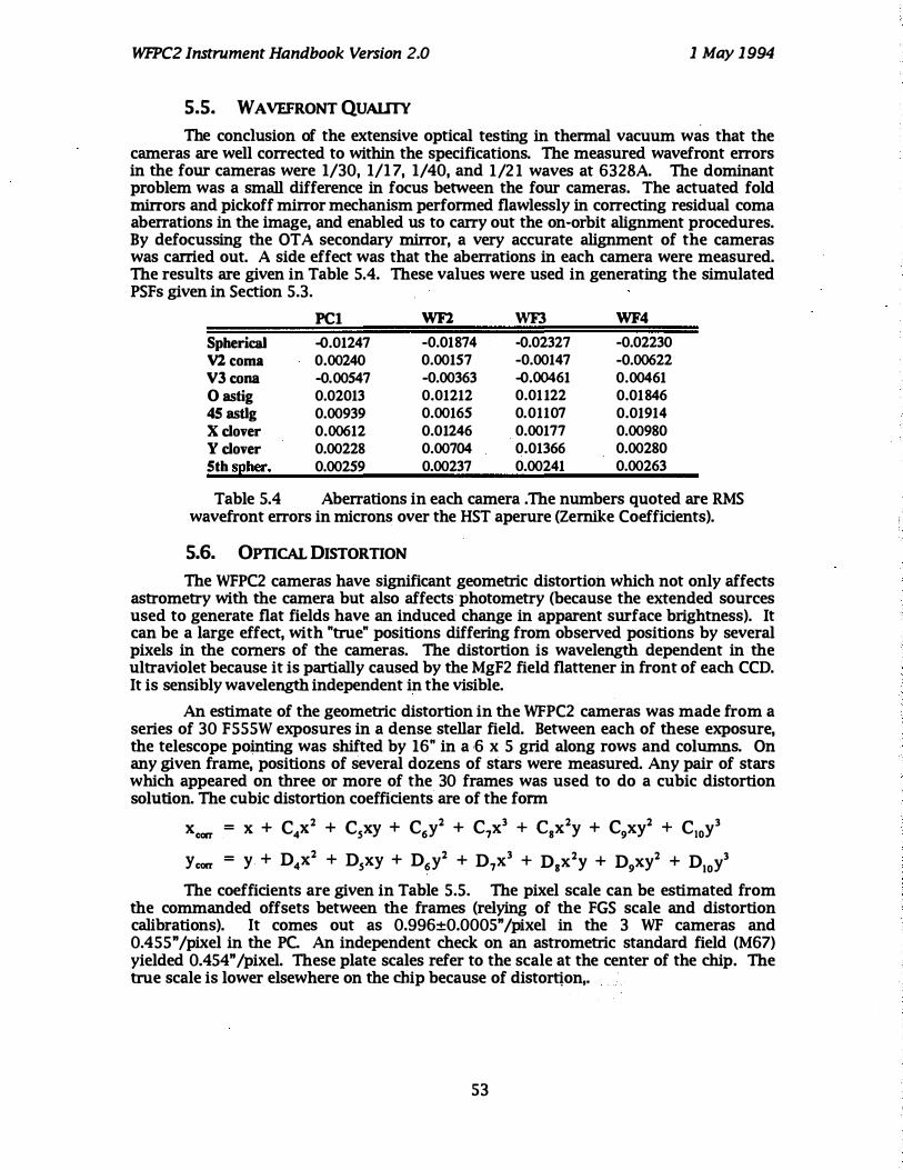
WFPC2 Instrument Handbook Version 2.0 1 May 1994
5.5. WAVEFRONT QUAUTY
The conclusion of the extensive optical testing in thennal vacuum was that the cameras are well corrected to within the specifications. The measured wavefront errors in the four cameras were 1/30, 1/1 7, 1/40, and 1/2 1 waves at 6328A. The dominant problem was a small difference in focus between the four cameras. The actuated fold mirrors and pickoff mirror mechanism perfonned flawlessly in correcting residual coma aberrations in the image, and enabled us to carry out the on-orbit alignment procedures. By defocussing the OTA secondary mirror, a very accurate alignment of the cameras was carried out. A side effect was that the aberrations in each camera were measured. The results are given in Table 5.4. These values were used in generating the simulated PSFs given in Section 5.3.
Spherical V2 coma V3 cona o astig 45 astlg X clover Y clover 5th spher.
PCI WF2 WF3 WF4
-0.01247 -0.01874 -0.02327 -0.02230
0.00240 0.00157 -0.00147 -0.00622
-0.00547 -0.00363 -0.00461 0.00461
0.02013 0.01212 0.01 122 0.01846
0.00939 0.00165 0.01107 0.01914
0.00612 0.01246 0.00177 0.00980
0.00228 0.00704 0.01366 0.00280
0.00259 0.00237 0.00241 0.00263
Table 5.4 Aberrations in each camera .The numbers quoted are RMS wavefront errors in microns over the HST aperure (Zernike Coefficients).
5.6. OPTICAL DISTORTION
The WFPC2 cameras have significant geometric distortion which not only affects astrometry with the camera but also affects photometry (because the extended sources used to generate flat fields have an induced change in apparent surface brightness). It can be a large effect, with "true" positions differing from observed positions by several pixels in the corners of the cameras. The distortion is wavelength dependent in the ultraviolet because it is partially caused by the MgF2 field flattener in front of each CCD. It is sensibly wavelength independent in the visible.
An estimate of the geometric distortion in the WFPC2 cameras was made from a series of 30 F555W exposures in a dense stellar field. Between each of these exposure, the telescope pointing was shifted by 16" in a ,6 x 5 grid along rows and columns. On any given frame, positions of several dozens of stars were measured. Any pair of stars which appeared on three or more of the 30 frames was used to do a cubic distortion solution. The cubic distortion coefficients are of the fonn
XCCIIT = x + C4X2 + CsXY + C6y2 + C,x3 + Csx2y + Cgxy2 + CIOy3
Ycorr = y + D4X2 + DsXY + D6y2 + D,x3 + Dsx2y + Dgxy2 + D)oy3 The coefficients are given in Table 5.5. The pixel scale can be estimated from
the commanded offsets between the frames (relying of the FGS scale and distortion calibrations). It comes out as 0.996±0.0005" /pixel in the 3 WF cameras and 0.455" /pixel in the Pc. An independent check on an astrometric standard field (M67) yielded 0.454" /pixel. These plate scales refer to the scale at the center of the chip. The true scale is lower elsewhere on the chip because of distorqon,.
53

WF.PC2 Instrument Handbook Version 2.0 1 May 1 994
PCl WFl WF3 WF4 C4 S.724E-OS -1.72SE-06 2. 626E-07 -6.933E-07 CS 6.442E-OS -1 .303E-06 -1. 104E-06 -1. 13SE-06
C6 -S. 1 13E-07 1 . 664E-07 9. 479E-07 S.3SSE-07 C7 -3.S72E';'()S -3.444E-OS -3.409E-OS -3.610E-OS
C8 1.036E-09 -4.S34E-IO -1 .S63E-I0 -1 .S79E-IO
C9 -3.637E-OS -3.40lE-OS -3.S3 1E-OS -3.490E-OS
CI0 -3.371E-IO -2.224E-I0 1.63 1E-I0 -4.7SSE-I0
D4 -1.099E-06 6. 149E-07 7.SS1E-07 S.S34E-07
DS -6. 1 16E-OS -2.2SSE-06 -1. 224E-06 -1.639E-P6
D6 3. S47E-07 -4.8S7E-07 -2.429E-07 -1.6SSE-07
D7 S.366E-12 2.43S-10 3.030E-I0 2. 37SE-l 1
D8 -3.477E-OS -3.470E-OS -3.S02E-OS -3.S13E-OS
D9 4. 104E-IO -1.760E-IO 6.916E-l l -1 .07SE-09
DI0 -4.1 1SE-OS -3.363E-OS -3.4S0E-OS -3.60lE-OS
Table 5.5 Cubic Distortion Coefficients
The cubic distortion coeffIcients can be used to derive effective pixel areas as presented in Figure 5.3. Contours are shown at half percent levels. Measurements of total brightness (as opposed to measurements of surface brightness), should be corrected by multiplying by the maps.
['.:1M Figure 5.3 Integrated Photometry Correction induced
by camera distortions.
54

WfPC2 Instrument Handbook Version 2.0
6. EXPOSURE TIME ESTIMATION
6.1. SYSTEM THROUGHPUT
1 May 1994
A decision on a suitable exposure time will require the combination of
a. The overall spectral response of the system (Figure 2.4).
b. The spectral transmission of the filters (Chapter 3 and Appendix 8.1).
c. The spectral energy distribution and spatial profile of the target.
d. The point response function and pixel size of the instrument (Chapter 5).
e. Criteria for specifying desirable charge levels.
When the transmissions of filters T(l) are combined with the overall system response Q(l), we obtain detective quantum efficiency plots (electrons-per-photon as a function of l) for each filter. These DQE plots link the output of the CCD to the photon flux at the input to an unobscured 2.4 m telescope.
These calibrations exist in the STScI Calibration Data Base and are accessible with the STSDAS Synphot package or with the XCAL software. The XCAL and Synphot Users Guides should be consulted for further details. We include here a sufficient calibration for exposure planning. This calibration is not sufficient for accurate photometry, because only a few standard star observations were available when this version of the handbook was written, and those only in a few filters.
In Table 6.2 the dimensionless efficiency and the mean wavelength for each filter are tabulated together with the effective width, the equivalent Gaussian dimensionless width, the maximum transmission, the derivative of the mean wavelength with respect to spectral index, the pivot wavelength, average wavelength, and wavelength of maximum transmission. The parameters are defined as follows. The dimensionless efficiency is J Q(l)T(l)dll l The mean wavelength is defined in Schneider, Gunn, and Hoessel Ap. J., 264, 337 (1983)
J = exJ J Q(l)T(l) log" (l)dlI l] � ) Q(l)T(l}dll l This rather unconventional definition has the property that the correspondingly defined mean frequency is just c / X. It is in some sense halfway between the conventional frequency mean and the wavelength mean. The pivot wavelength is defined as [ J Q(l)T(l)Ml J/2 l
p = J Q(l)T(l}dll X
The effective Gaussian is defined implicitly by
u2 =[J ���� Q(l)T(l)log2 (l7 l» 2dl l lJ/2 ) ���� Q(l)T(l}dll l where the integration limits eliminate unrealistic contributions from imperfect blocking far from the passband. The effective width of the bandpass is
oX = 2[2 1og2 2]1/2 uX
55
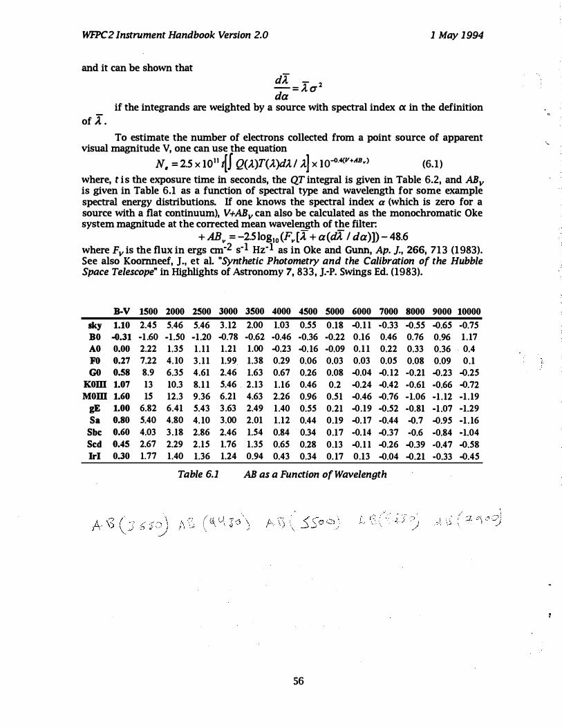
Wf1'C2 Instrument Handbook Version 2.0 1 May 1994
and it can be shown that iI -_= l 0" 2 da
if the integrands are weighted by a source with spectral index oc in the definition of I.
To estimate the number of electrons collected from a point source of apparent visual magnitude V, one can use the equation
N. = 2.5 x lOll t[f Q(l)T(l}dl/ l] x 10-o·4{v+ABv) (6.1)
where, t is the exposure time in seconds, the QT integral is given in Table 6.2, and ABy is given in Table 6.1 as a function of spectral type and wavelength for some example spectral energy distributions. If one knows the spectral index a (which is zero for a source with a flat continuum), V+ABy can also be calculated as the monochromatic Oke system magnitude at the corrected mean wavelength of the filter:
+ ABv = -2.5 1oglo (Fv [l + a(dX / da)]) - 48.6 where Fy is the flux in ergs cm-2 s-l Hz-1 as in Oke and Gunn, Ap. J., 266, 71 3 (1983). See also Koornneef, J., et al. "Synthetic Photometry and the Calibration of the Hubble Space Telescope" in Highlights of Astronomy 7, 833, J.-P. Swings Ed. (1983).
D-V 1500
sky 1.10 2.45 DO -0.31 -l .60 AO 0.00 2.22 FO 0.27 7.22 GO 0.58 8.9
KOm 1.07 13 MOm 1.60 IS
gE 1.00 6.82 Sa 0.80 5.40
Sbe 0.60 4.03 Sed 0.45 2.67 IrI 0.30 l.77
2000 2500 3000
5.46 5.46 3 .12
-l.50 -l.20 -0.78 l.35 l . 11 l.21 4. 10 3 . 11 1.99 6.35 4.61 2.46 10.3 8.1 1 5.46 .
12.3 9.36 6.21 6.41 5.43 3 .63 4.80 4. 10 3.00 3 .18 2.86 2.46 2.29 2.15 1.76 1.40 l.36 l.24
Table 6.1
( i \:i:. V , . , \
3500 4000 4500 5000 6000 7000 8000 9000 10000
2.00 l.03 0.55 0.18 -0.1 1 -0.33 -0.55 -0.65 -0.75 -0.62 -0.46 -0.36 -0.22 0.16 0.46 0.76 0.96 l .17 l.00 -0.23 -0. 16 -0.09 0.1 1 0.22 0.33 0.36 0.4 l.38 0.29 0.06 0.03 0.03 0.05 0.08 0.09 0.1 l.63 0.67 0.26 0.08 -0.04 -0. 12 -0.21 -0.23 -0.25 2.13 l.16 0.46 0.2 -0.24 -0.42 -0.61 -0.66 -0.72 4.63 2.26 0.96 0.51 -0.46 -0.76 -l.06 -l .12 -l .19 2.49 1.40 0.55 0.21 -0.19 -0.52 -0.81 -l .07 -l.29 2.01 l.12 0.44 0.19 -0. 17 -0.44 -0.7 -0.95 -l .16 l.54 0.84 0.34 0.17 -0.14 -0.37 -0.6 -0.84 -l.04 l.35 0.65 0.28 0.13 -0.1 1 -0.26 -0.39 -0.47 -0.58 0.94 0.43 0.34 0. 17 0.13 -0.04 -0.21 -0.33 -0.45
AB as a Function of Wavelength
., I · "
56
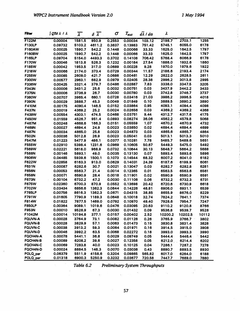
WFPC2 Instrument Handbook Version 2.0 1 May 1 994
FIl_ l QTd A. I A. :r- o T u TA£tX dl / da l F1 22M 0.00004 1 58 1 .5 950.9 0.2553 0.00034 1 03 . 1 2 21 98.7 2703.1 1 255 F1 30LP 0.09732 61 03.2 461 1 .2 0.3837 0. 1 3983 761 .42 6746. 1 6066.0 61 78 F1 60AW 0.00026 1 690.7 642.2 0.1 448 0.00066 33.33 1 626.0 1 642.5 1 797 F1 60BW 0.00026 1 690.7 642.2 0.1 448 0.00066 33.33 1 626.0 1 642.6 1 797 F1 65LP 0.09704 61 54.0 4493.3 0.3702 0. 1 41 08 706.42 6768.4 6066.9 61 78 F1 70W 0.00046 1 8 1 3.8 626.3 0.1 232 0.00 1 84 27.64 1 886.0 1 932.6 1 860 F1 86W 0.00042 1 953.6 31 7.0 0.0689 0.00228 9.28 1 970.0 1 979.6 1 922 F218W 0.00066 21 74.0 373.4 0.0729 0.00344 1 1 .67 21 86.6 21 93.4 2 1 74 F255W 0.00085 2609.0 421 .7 0.0686 0.00461 1 2.29 2622.0 2628.6 261 1 F300W 0.00677 2963.1 682.9 0.0979 0.02405 28.38 2996.2 301 3.8 2996 F336W 0.00426 3321 .4 379.7 0.0486 0.02887 7.83 3338.0 3347.6 3205 F343N 0.00006 343 1 .2 25.6 0.0032 0.00751 0.03 3437.9 3442.2 3433 F376N 0.00006 3736.9 26.7 0.0030 0.00780 0.03 3742.8 3746.7 3737 F380W 0.00707 3965.4 680. 1 0.0728 0.0341 6 21 .03 3986.2 3996.6 401 8 F390N 0.00029 3888.7 45.3 0.0049 0.01 849 0. 1 0 3889.5 3890.2 3890 F410M 0.00 1 75 4090.4 1 46.5 0.01 52 0.03864 0.95 4093.1 4094.4 4098 F437N 0.0001 9 4369.2 25.2 0.0024 0.02656 0.03 4369.2 4369.2 4368 F439W 0.00554 4303.1 474.5 0.0468 0.03751 9.44 431 2.7 431 7.6 41 75 F450W 0.01 559 4526.7 951 .4 0.0893 0.08274 36.06 4562.2 4579.8 5068 F467M 0.00248 4668.6 1 66.3 0.01 51 0.05559 1 .07 4670.2 4670.9 4732 F469N 0.00027 4694.4 24.9 0.0023 0.03850 0.02 4694.4 4694.4 4699 F487N 0.00034 4865.0 25.8 0.0023 0.04873 0.03 4865.6 4865.7 4864 F502N 0.00036 501 2.8 26.9 0.0023 0.05041 0.03 501 3. 1 601 3.3 501 0 F547M 0.01 223 5477.9 486.1 0.0377 0.1 0281 7.78 5485.7 5489.6 5651 F555W 0.0291 0 5398.4 1 231 .6 0.0969 0.1 0605 50.67 5449.3 5475.0 5492 F569W 0.02221 561 8.0 968.9 0.0732 0. 1 0644 30. 1 3 5648.7 5664.2 5688 F588N 0.00 1 46 5893.1 49.0 0.0035 0. 1 3 1 30 0.07 5893.4 5893.6 5896 F606W 0.04485 5939.6 1 500:1 0.1 073 0.1 4544 68.32 6007.2 6041 .0 6 1 82 F622W 0.02858 61 63.3 91 3.0 0.0629 0. 1 4031 24.39 61 87.6 61 99.9 6061 F63 1 N 0.00087 6282.6 30.7 0.0021 0.1 3047 0.03 6282.7 6282.8 628 1 F656N 0.00053 6563.7 21 .4 0.00 1 4 0.1 2365 0.01 6563.5 6563.6 6561 F658N 0.00071 6590.9 28.4 0.00 1 8 0.1 1 901 0.02 6590.9 6590.9 6591 F673N 0.00 1 04 6732.2 47.2 0.0030 0.1 1 1 06 0.06 6732.2 6732.3 6731 F675W 0.02360 6700.3 870.9 0.0552 0. 1 3698 20.42 6720.6 6730.9 661 8 F702W 0.03434 6856.6 1 362.3 0.0844 0.1 4226 48.8 1 6906.0 693 1 . 1 6539 F785LP 0.00756 861 6.3 1 362.3 0.0671 0.0431 5 38.85 8655.9 8676.0 8229 F791 W 0.01 605 7790.9 1 1 89.3 0.0648 0. 1 001 8 32.74 7824.2 7841 . 1 7374 F81 4W 0.01 822 7877.5 1 469.0 0.0792 0.1 0970 49.40 7928.6 7954.7 7247 F850LP 0.00364 9089. 1 1 01 9.6 0.0476 0.03095 20.63 91 1 0.2 91 20.8 8766 F953N 0.0001 0 9528.9 67.3 0.0030 0.01 432 0.09 9536.8 9539.7 9528 F1 042M 0.0001 4 1 01 94.8 377.1 0.01 57 0.00402 2.52 1 0200.2 1 0202.5 1 01 1 2 FQUVN-A 0.00028 3764.9 73. 1 0.0082 0.01 1 26 0.26 3765.9 3766.7 3802 FQUVN-B 0.00028 3829.9 57.1 0.0063 0.01 473 0. 1 5 3830.8 383 1 .4 3828 FQUVN-C 0.00038 391 3.2 59.3 0.0064 0.01 971 0. 1 6 391 4.5 391 5.0 3908 FQUVN-O 0.00046 3992.2 63.5 0.0068 0.02272 0. 1 8 3993.0 3993.3 3990 FQCH4N-A 0.00078 5441 . 1 36.8 0.0029 0.09749 0.05 5444.4 5446.4 5442 FQCH4N-B 0.00089 6208.2 39.6 0.0027 0.1 2358 0.05 621 2.0 621 4.4 6202 FQCH4N-C 0.00069 7283.8 40.0 0.0023 0. 1 0 1 25 0.04 7286.1 7287.2 7278 FQCH4N-O 0.00024 8884.5 1 46.3 0.0070 0.03038 0.43 8890.7 8893.5 8930 POLQ_par 0.06379 551 1 .9 41 58.6 0.3204 0.09865 565.82 601 7.0 6264.0 6 1 88 POLQ per 0.01 3 1 8 6900.3 5250.9 0.3232 0.03677 720.58 7447.7 7689.0 7880
Table 6.2 Preliminary System Throughputs
57

WfPC2 Instrument Handbook Version 2.0 1 May 1994
6.2. SKY BACKGROUND
The actual sky brightness depends on the heliocentric ecliptic latitude and apparent longitude, in a manner summarized in Table 6.3. The appropriate ABv can be taken from Table 6.1. To convert magnitudes/arcsecond2 to magnitudes/pixel2 one needs to add 5 (WFC) or 6.7 (PC1).
Eclintic Latitude Apparent 0 30 60 90 Lons!tude
180 22. 1 22.7 23.2 23.3
145 22.4 22.9 23.3 23.3
110 22.3 22.9 23.3 23.3
Table 6.3 Sky Brightness (V magnitude/arcsecond2) as a Function of Ecliptic Latitude and Apparent Longitude
6.3. POINT SOURCES
The signal to noise ratio for a point source in the normal read noise or background limited case is a function not only of the expected number of detected photons 1 from the source but also of the average background count rate in each pixel B, the point spread function P(iJ), and the weights used to average the signal in the pixels affected by the source. It is easy to show that the signal to noise ratio for optimal weights (which are proportional to the point spread function) is given by
(S I N)2 = � LP(i,j)2 (6.2)
The sum on the right is tabulated for a few representative cases in Table 6.4 To estimate the signal to noise, multiply the signal to noise obtained assuming all the flux is in one pixel by the square root of the value in the Table.
2000 A 4000 A 6000 A 8000 A Obs. Diff. Obs. Diff. Obs. Diff. Obs. Diff.
PC Center 0.040 0.41 1 0.073 0.253 0.058 0.1 1 3 0.043 0.072 PC Comer 0.033 0.1 96 0.051 0.1 08 0.048 0.072 0.042 0.067 WF Center 0.1 24 0.740 0.145 0.481 0.127 0.31 8 0 .123 0.281 WF Comer 0.1 02 0.279 0.1 06 0.206 0.099 0.1 82 0.082 0.1 28
Table 6.4 Sharpness as a Function of Wavelength, Camera, and PIXel Phase With and without Instrumental Effects.
For example, Table 2 .2 lists the faintest V magnitude star measurable with a signal to noise ratio of 3 in a 3000s integration in F569W in the wide field cameras. The calculation to check this goes as follows. The efficiency of the filter is 0.022 2 1 from Table 6.2. The sky background in each pixel is 22.3+5=28.3 assuming an ecliptic latitude of 90' from Table 6.3, and the pixel area correction for the WFC given in the text above that Table. The total sky background collected per pixel in 3000 seconds is given by Equation 6.1 as 79.7 electrons. Note that the AB color correction required for the sky in the wavelength range of the filter is 0.0 from Table 6.1. From Table 4.3, the read noise is 5.2 electrons. From Table 4.2, the median dark current at -77C is 0.016. Therefore the total median dark current (on which there will be shot noise is) 48 electrons. The equivalent background per pixel is then given as B=79.7+5.22+48=1 54.8. The total number of detected electrons from a star with V=27.99 is 1=88 electrons, again using equation 6.1. The expected peak count is 3 1 detected electrons using Table 5.2, which is much less than B, allowing the use of Equation 6.2. (If it comes out much
58
",
I ' I

WfPC2 Instrument Handbook Version 2.0 1 May 1994
greater as it can in UV filters, one is not read or background limited, but photon noise limited. Then the signal to noise comes out as the square root of I). The sharpness for the WF camera in the best case when the star is centered on a pixel is given in Table 6.4 as 0.123. Then Equation 6.2 above gives the signal to noise as 3.0.
In principle, one should also include contributions in the signal to noise for flat fielding uncertainties, dark frame errors, and quantization noise. Flat fielding errors will be of order 196. Dark frame errors in the vast majority of pixels seem to be small (with the expected poisson statistics). Quantization noise can be treated accurately by adding a term G2/1 2 to the background rate B (ie 4.1 in the 7 electron channel, and 16.3 in the 14 electron channel)
6.4. ExTENDED SOURCES
In general, the signal to noise level for extended sources is computed for each pixel. The sources of noise are read noise, sky background, flat field residuals, and photon noise. If read noise is the dominant noise source, the signal to noise can be improved by using AREA mode (see page 13), at some cost in resolution. Observers are encouraged to simulate the expected image in order to optimize their observations.
For high-z galaxies, a much smaller fraction of light falls in the central pixel than for a point source of equivalent total flux. The rough magnitude difference between the light falling in the central pixel and the entire galaxy is plotted against redshift in Figure 6.1, for giant elliptical galaxies. For other types of galaxies, a morphological term can be added to the values in for example, 0.6 magnitudes for lenticulars, 0.7 for S, 0.8 for Sab, 0.9 for Sbc, 1.2 for Sed, and 1.8 for 1m. These values must be increased by an additional 1 .7 magnitudes for the Pc.
Wide Field : Mean O<q<+O.5 3.0 ....-,.--...,.--.----r----,.---.r--..-- -r---.-'-'-r----.-'----,--r--'--.-"--,-.:..:.,....---.----.--r---r---.-'---r----.-----,r---,
� 3.5 E "
� '" � ...!.. I 1
"" "
� 4.0
Redshift Z
Figure 6.1 Giant Elliptical Galaxy
59
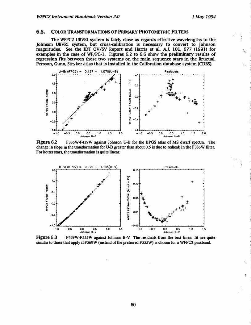
WfPC2 Instrument Handbook Version 2.0 1 May 1 994
6.S. COLOR TRANSFORMATIONS OF PRIMARY PHOTOMETRIC FILTERS
The WFPC2 UBVRI system is fairly close as regards effective wavelengths to the Johnson UBVRI system, but cross-calibration is necessary to convert to Johnson magnitudes. See the lOT OV/SV Report and Harris et al. A.J. 101, 677 (1991) for examples in the case of WF /PC-I. Figures 6.2 to 6.6 show the preliminary results of regression fits between these two systems on the main sequence stars in the Bruzual, Persson, Gunn, Stryker atlas that is installed in the Calibration database system (CDBS).
U-B(WFPC2) = 0.1 27 + 1 .070(U-B) 2.0
I .S
� 1 .0 .... • ... I � o.S .... .... ... +. '" � 0.0 � Of-
..... -o.S + -#
- 1 .0 L.....""---'--�...L.....� ........ _ ........ _--'-� ...... - 1 .0 -0.5 0.0 0.5 1 .0 1 .5 2.0
Johnson U-8
] � is � ;!
0.2
0.0
� -0.2 co .... .... ... '" � -0.4 �
Residuals
+
+ - 0 . 6 '--_ ......... � .......... _ ......... _ ....... _ ........... �.......J
- 1 .0 -0.5 0.0 0.5 1 .0 1 .5 2.0 Johnson U-B
Figure 6.2 F336W-F439W against Johnson U-B for the BPGS atlas of MS dwarf spectra. The ' change in slope in the transformation for U-B greater than about 0.5 is due to redleak in the F336W filter. For hotter stars, the transformation is quite linear.
B-V(WFPC2) = 0.029 + 1 . 1 45(B-V) I .S +
�
� '6 " It'> ! It'> ... I is iJ: It'> 01 on .... It'> • ... ... I '" iJ: � 01 .... � ... ... N 0 II. �
- 1 .0 -0.5 0.0 0.5 1 .0 1 .5 Johnson 8-V
Residuals 0.1 5
0.10
0.05 \ + *
... * + * ++++
0.00
-0.05 - 1 .0
\ +++ �4(�
-0.5 0.0 0.5 Johnson 8-V
+
1 .0 1 .5
Figure 6.3 F439W-F555W against Johnson B-V The residuals from the best linear fit are quite similar to those that apply ifF569W (instead of the preferred F555W) is chosen for a WFPC2 passband.
60

WfPC2 Instrument Handbook Version 2.0
V-I(WFPC2) = 0.078 + O.B85(V-I) 2 ��������������
� ... iii ... i on 0 on on ... N � ... �
- 1
-2 -2 - 1 0 2
Johnson V-I
"0 " ! 0.02 � ... iii ... I � 0.00 on on ... N � -0.02 l
-0.04
Residuals
*+ �++ "t.-H:t-+ + �+� + :t+ +* + +.\: + '1-+ +
+
+ � +
++
-2 -1 0 Johnson V-I
1 May 1994
+
:\:. + +
2
Figure 6.4 FSSSW-F814W against Johnson V-I The residuals from the best linear fit are generally very small. This particular color combination is widely used.
V-R(WFPC2) = -0.0 1 8 + 0.895(V-R) Residuals 1.0 0.10
+ :;- �"\ + ... 0.05
:# +:1=+ 0.5
� "0 / � " 0.00 ... 0 '" � ... I � � on * on !O -0.05 f on on ... ... I N � U on Q. :fl -0.10 l ... +
N + U e: -0. 1 5 � + -0.20
- 1 .0 -0.5 0.0 0.5 1 .0 1 .5 - 1 .0 -0.5 0.0 0.5 1 .0 1 .5 Johnson V-R Johnson V-R
Figure 6.5 F55SW-F67SW against Johnson V-R The residuals from the best linear fit are somewhat larger for blue stars (V-R<-O.6) than those that apply ifF569W is chosen.
R-I(WFPC2) = 0.095 + O.876(R-I) Residuals 1 .0 0.20 + + ++ if 0.1 5 + � is ... "
0.1 0 iii ! ... + I � �� � on ... ... iii 0.05 If ... '*' 1 #" I N � � ... 0.00 l '" ... N U e: -0.05 + ++ �
- 1 .0 -0.10 - 1 .0 -0.5 0.0 0.5 1 .0 - 1 .0 -0.5 0.0 0.5 1 .0
Johnson R-I Johnson R-I
Figure 6.6 F67SW-F814W against Johnson R-I The residuals from the best linear fit are similar to those that apply ifF791 W is chosen for a WFPC2 I passband. For spectral type M8V and later (not shown) the transformation will not work as well.
61

WFPC2 Instrument Handbook Version 2.0
6.6. RED LEAKs IN W FILTERS
1 May 1994
The "red leaks" in the UV filters are shown in Figure 6.7 for F122M, F160W (the new Woods filter), F1 70W, F18sW F2 18W F2s sW, F300W and F336W. The presence of significant red leaks in the UV filters, together with the much greater sensitivity and wavelength coverage in the red part of the spectrum, makes calibration of UV observations difficult. Table 6.5 shows preliminary red leak estimates as a percentage of the total detected flux from dereddened stellar sources ordered by spectral type. In each column, the red leak is defined as the percentage of the detected flux longward of the cutoff wavelength in the second row. In the presence of interstellar reddening, the red leaks will be larger.
Q) en F 1 22M g _ 1 r-����--�--�� � -2 <11
c::: - 3 � - 4 � -5 � _____ , e -6 ""'" � -7 a-��� ____ � __ � �� g' 2000 4000 6000 80001 0000
...J Wavelength (Angstroms) "....... � F 1 70W 8.. - 1 li'l -2
c::: - 3 � -4 (ij -5 >-e - 6 � -7 ���� ____ � __
��
.3 2000 4000 6000 80001 0000 Wavelength (Angstroms)
"....... � F2 1 8W 8.. - 1 li'l - 2
c::: - 3 E - 4 <11 � -5
e - 6 � -7 ����� __ ���� .3 2000 4000 6000 80001 0000
Wavelength (Angstroms) "....... � F300W 8.. - 1 li'l - 2
c::: - 3 E -4 <11 � -5
e - 6 � -7 ���� __ ��
__ ��
g' 2000 4000 6000 80001 0000 ...J Wavelength (Angstroms)
"....... � F 1 60BW (WOOdS) o - 1 � -2 <11
c::: - 3 E - 4 � I/) - 5 >-
e - 6 � - 7 ��� __ � __ � ____ �
g' 2000 4000 6000 80001 0000 ...J Wavelength (Angstroms) "....... <11 I/) c: o - 1 � - 2 <11
c::: - 3
F 1 85W
� -4 � -5 e - 6 � - 7 LL __ ��==�"�� .3 2000 4000 6000 80001 0000
Wavelength (Angstroms) "....... � F255W 8.. - 1 li'l - 2
c::: - 3 E -4 <11
til - 5 >-e -'- 6 � -7 �� __ �� __ � ____ � g' 2000 4000 6000 80001 0000 ...J Wavelength (Angstroms) "....... � F336W o - 1 � -2 <11
c::: - 3 E - 4 <11 til - 5 >-e - 6 � -7 ��� __ ��-L� __
J
g' 2000 4000 6000 80001 0000 ...J Wavelength (Angstroms)
Figure 6.7 UV Filter Red Leaks including the on-orbit measurements of system response.
62
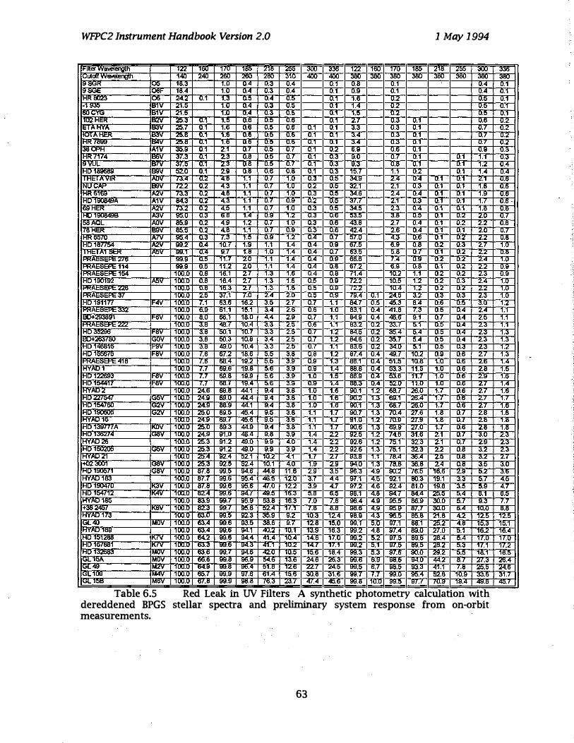
WfPC2 Instrument Handbook Version 2.0 1 May 1 994
! FiKer Wavelength 122 160 170 1110 2111 205 .)UIJ ;,� 1-" 160 170 1110 2111 .. :tE ;,uu ,Cutaf WMlength 140 240 260 260 260 ;'1V 'lUI) 'lUI) .xsu .xsu 380 380 380 � 380 19 SGR u:> 111.3 .V U.4 U.3 V.4 U. V.II V. 0.4 19 SGE UtII- 111.4 .U U.4 U.3 �4 _U.l � � 0.4 IHR &l23 06 24.2 0.1 1.3 U.O U.4 U.O U.1 1.1'; .U.2 0.5 -1 935 BW 21.5 1.U U.4. U.3 U.O U.1 . 104 ...11,2 . 0.5 I60 CYG !BW 21.5 1.U 0.4 U.3 U.5 U.1 1.5 .U.2. 0.5 1102 HER 1B2V 25.3 0.1 1.5 0.6 U.5 0.6 0.1 . 2.7 .U.3 . U.1. ·0.6 IETAHYA !B3V 25.7 0.1 1.6 0.6 U.5 U.6 0.1 0.1 3.3 U.3 U.l 0.7 IIOTARER II:S3V 25.8 0.1 1.6 0.6 0.0 v.o u. U. ;'.4 0.3 0.1 U.7 IHK 1t11i9 ItI4V :to.1I U. .0 V.O U.O v.o V. V. ".4 U." V. U. 138 OI-'H lAW 30.9 0.1 2.1 0.7 V.O u. U. U.:t 0.9 v.o V. U.9 IHR 7 74 II:!6V 37.3 U. 2.3 U.II U.O U. U. U.3 9.U . U. u. 19 VUL 11:!7V 37.5 U. 2.3 U.II U.O U. U. U.3 9.3 U.II V. .1 1.2 IH0 1B9689 IB9V 52.0 0.1 2.9 U.II V.I) .11,11 U.l .. U.3 E·t .... 1 . _U.;.!. . 1 1.4 ITHETAVIR IAOV 73.4 0.2 4.6 1.1 U.I 1.U U.3 U.O _34.9 .2.4 U.4. .U..! .1 2.1 INU CP<P IB9V 72.2 0.2 4.3 1 .1 U.7 1.U U.2 U.5 32.1 2,1 U.3 U.l .1 1.8 IHR 5159 IA2V 13.3 U.2 4.0 .1 0.7 1 .0 0.3 0.5 34.6 2.4 0.4 U. 1 .9 IH0 19U849A lAW 114.3 U.2 4.3 .. 1 0.7 0.9 0.2 0.5 37.7 2.1 v.;, JI.2 .1 1.7 169 HER IA2V 73.2 U.2 4.0 1.1 U.I ).u .U.3 U.O � __ O. �3. y.4. U-.1.. .1 1.8 IH019U849B IA3V 95.0 0.3 6.11. 1� 1).9 .... 2 _U.3 _U.5 � � � _U..! 1.2 ·2.0 I58ACL IAOV 85.9 0.2 4.9 1.2 UJ 1.U U.3 U.5 _43.11 2.1 U.4. U .. l 1.2 2.2 1/11 Ht:K II:!9V 85.5 0.2 4.11 1.1 U.7 U.9 U.3 U.6 _42.4 .2.6 U.4. u..! .1 ·2.0 IHR657U- IA7V 95.4 0.3 7.3 1.5 U.9 1.2 U.4 U.7 07.U 4.3 U.6 U.l 1.2 2.2 IH0 1117754 IA2V 99.2 U.4 10.7 1.9 1.1 1 .4 0.4 0.9 67.5 6.9 U.II 0.2 1.3 2.
1 Ht: 1 A' lOt:K IAOV 99. U.4 9. 1 1.11 1 .V 1 .4 V.'+ V. 0".0 0.0 U.I U. 1.:t 2.2 : 2/5 99.9 U.O 11.7 2.0 1 .1 1.4 0.4 0.9 511.6 7.4 0.9 0.2 1.2 2.4
114 99.9 U.O .2 ;l.0 1 .1 1.4 0.4 0.8 67.2 6.9 V.O U. 1.2 2.2 104 loo.U O.B 16.1 2.7 1.3 1 .6 0.4 0.8 71.4 1U.2 1.1 0.2 1.2 2.3
IHO 190192 IAOV loo.U U.II 16.'+ :t. 1 .3 1.0 V.O U.9 12.2 lU.O .2 V.2 1.3 2.4 : 22ti loo.U U.II 11)." 2. I." 1.0 V.O V.9 12.2 lUA .2 V.2 1.2 2.2 : 3( loo.U 2.0 3/. 7.v 2A 2.0 0.5 0.9 19A V. 2'+.0 3.:t U." 1.3 2.3
IH0 19' 1Tf IF4V 100. 53.0 16.:t 3.0 :t. U. 114.1 1.0 40.3 11.4 1.0 1.5 3.0 : 332 loo.U 6.9 6' . 10. 3.4 :t.6 Jl.ti _1.U � � � � � 1.4 2.4
180+293891 IF6V 100.0 8.0 66.1 111.U 4.4 2.9 UJ 1 .1 .114.9 UA .4t:i.ti. 9.1 U.I 1.4 2.5 : 222 100.0 3.8 48.1 lU.4 3.3 2.0 U.5 1.1 .113.2 U.2 33.1 0.1 U.O 1.4 ·2.3
IH0 35296 IF8V 100.0 3.B 50.1 10.7 3.3 2.5 U.7 1.2 114.5 U.2 35.4 5.4 U.O 1.4 ·2.3 180+263780 IGOV 100.0 3.B 50.3 10.8 3.4 2.5 0.7 1.2 114.6 U.2 35.7 5.4 0.5 1.4 2.3 IH014t:i!11ti -9V 1OO.U 3.11 49.V lU.'+ ".;, 2.0 V. 0".0 V.2 -'4.U O. V.O J.3 2.3 IH0 105670 Il-tlV loo.U '.5 5/.:t 111.ti .� �tI _u.tI _1.2 ..tI.f.'I. � � .'1.U� � 1.6 2.7
: 41t1 loo.U 1.5 511 . ." 19-<!. 0,0 . 3.9 ..0.9 1 .3 � ...1-1.4. JI.l.0 . .1U.1I. 1,1) 11.6 2.6 IHYAD l 100.0 7.7 69.ti 19.tI 0.5 3.9 U.9 1.4 tIII.tI U.4 03.3 11.0 1.U 1.6 2.B IH0122693 !FBV 100.0 7.7 69.11 19.9 5.6 3.9 1.0 1.5 88.9 U.4 53.6 11 .7 1.U 1.6 -2:9· IHOl544f7 I"OV 100.0 7.7 68.7 19.4 5.6 3.9 U.9 1.'+ 00." U.'+ 02.U I.U I.U J.ti 2.1 IHYAD2 1 100.0 24.6 88.8 44.1 9.4 3.8 1.0 1.6 90.1 1 .2 00. 2tI.U J.5 2.7 IHD227� luOV loo.U :t4.9 tI9.V qq.,+ 9.'+ ".0 I .U 1.0 90.2 I ." 09. 2tI.'+ J.5 2. IHD154750 lu2V loo.U 24.9 tIII.9 qq. 9.4 3.tI I.U I.ti 9O..! 1.3 titI:.{ � � 1.6 2.7 IH0 19U600 IG2V loo.U 25.U 69.,:>, 40.." �o .3 __ tI 1.1 1.1 �I 2-3. --'.0,4. _21.ti. 1"'- 1.7 2.8 I HYAD 15 loo.U 24.9 69.1 4O.ti 9.0 .� ].1 _1.1 � E �. �.� � 1.7 2.8 IH0 13977fA IKUV 100.0 25.U 69.3 44.9 9.4 3.tI 1.1 1.7 .90.5 1.3 . t:i9.9. 2/.U 1./ 1.6 2.8 IHO l36274 IGIIV loo.U 24.9 91.U 4tI.4 9.tI 3.9 1.4 2.2 92.0 1 .2 . 14.0 31.ti 2.1 1.7 ·3.0 IHYAD 26 100.0 25.3 91.2 49.U 9.9 4.U 1.4 2.2 92.5 1.2 75.1 32.3 2.1 1.7 ·2.9 IHO l50205 IG5V ! 100.0 25.3 91.2 49.0 9.9 3.9 1.4 :t.:t 92.0 1 .3 � 32.3 :t.2 1.11 3.2 HYAU :t1 loo.U :to.4 9'2.'+ 02. 1U.2 4. 2. 93.11 IliA �.'+ 2.0 1.8 3.2 1+02300f utlV loo.U 20.3 9'.l.o .o:t--". 1.11,1 _4.U 1.9 2.9 JI<tU ).3. JII.II_ .3t:i.1I. .2.-". 11.8 3.5 'HD l9U5r utlV loo.U tl/.tI 99.� . 94-.t' q<j.tI '11.ti 2.9 3.0 JIti.3. 59 .9O.:t_ lti.� 1o.ti ;l.9 5.2 .HYAD 183 100.0 87.7 99.5 95.4 40.0 12.U 3.7 4.4 9(.1 4.5 92.1 60.3 19.1 �.3 5.7 IH0 190470 K3V 100.0 87.8 99.5 95.5 47.0 12.2 3.9 4.7 97.2 4.6 92.'+ O·I.U 19.0 .i.5 5.9 H0 154712 ,,'+v 100.0 82.4 99.6 94. 1 '+9.0 10.3 0.11 0.0 911. '+.11 9'+. �'+ :to.O 0.4 11.1 ,HVAD185 loo.U 113.9 99. 90.9 OJ.tI '1..0,-3 l.U l.ti JIlI __ 4 . ....".9. _90.0_ .tIt:i.� .3O-,-U. 0.7 9.3 +38 2407 KtlV loo.U tl2.3 99.1 90.11 0:t.4 '1.'..1 J..tI _tl.tI � --"".9. �-,9 _ _ tl/.1.. .3O..-lI. ci.4 10.0 HYAD 73 100.0 53.U 99.0 92.3 30.9 9.2 lU.3 12.4 911.9 4.3 95.5 85.11 21.11 4.2 12.5 IGL40 MOV 100.0 63.4 99.5 93.5 38.6 9.7 12.8 15.0 99.1 5.0 97.1 88.1 20.2 4.tI 15.3 IHYAD 189 100.0 63.4 99.6 94. qu.2 lV. 1".11 10.3 99.2 '+.11 9'.-". �V 2, .U 0.1 16.2 ,HO 151288 .r<.,v 100.0 ti4.:t 99.t> 9'+.'+ '+, .4 lU.4 14.ti 'It·u � � Jl.l..0 _ _ tI9.1l. _:tIS:". 0.4 17.0 IRD lo/tlll' "'V loo.U 1)3.3 99.0 9'+.3 '+1 . lU.2 14.1 '1/'.1 � � JI0I_ �� �� 0.3 17.1 'H0 132583 MUV loo.U 53.6 99. _94..ti. .� '1IJ.0 10.ti lt1.4 JI!:I.3. _0.3 . . 9/.0_ 9O.!J. 29 •. 2 0.5 18.1 IGL 15A 'MUV 100.0 66.5 99,t1 95 .. 9 04.6 13.5 24.6 26.3 . 99.5 5.9 . 98.5 94.U 44.2 11.7 ·27.3 IGL 49 M2V loo.U 114.9 99.11 .95.-". O ..... tI '12.5 22.7 24.5 _99.0 .5.l 911.0 93.3 ,+., . '.11 :to.o IGL 109 IM4V 100.0 65.7 99.9 97 .. 5 51.4 10.5 30.8 31 .6 . 99.7 f.7 99.U 95.4 52.8 111.9 --s3:6 IGL 15B IM5V loo.U 57.tI 99.9 9II.tI .� �l .41.4 45.6 J:l!i.8. )U.U _ _ 99.0_ . 97.1.. IU.>J ·,01.4 49.ti
Table 6.S Red Leak in UV Filters A synthetic photometry calculation with dereddened BPGS stellar spectra and preliminary system response from on-orbit measurements.
63
336 380 0.1 0.1 0.1 O�f o.r U.2 � 0.2 U.2 0.3 0.3 0.4 0.4 0.6· 0:0 0.6 0.6 · 0.6 0.7 0.8 0:7 O.s-I.U U.II I.U U.9 U.9 1.0 1.0 1.0 1.2 1 .1 1.1 1.1 1.3 1 .3 1.2 1.3 1.4 1.5 1�o 1 .4 1.6 .. 7
1 .6 1.8 1.8 1.8 2.3 2.3 2.3 2.7 3.0 3.6 4.5 4.7 6.5 7.7 8.8 12.5 15:1 16.4 17.0 17.2 18.5 26.4 24.5 31:7 40.1

WfPC2 Instrument Handbook Version 2.0
7. CALIBRATION AND DATA REDUCTION
7.1. CAuBRATION OBSERVATIONS AND REFERENCE DATA
1 May 1994
Standard calibration observations are obtained and maintained in the HST archive at the STScI, and can be obtained by external users using StarView. This includes those flat field, dark and bias frames needed to operate the Post Observation Data Processing System (PODPS; usually just called the "pipeline"), a photometric calibration derived from standard star observations and the measured filter profiles, and derived determinations of the plate scale, distortion, and so on. The first set of these calibrations were provided to the STScI by the WFPC2 IDT from the Servicing Mission Observatory Verification (SMOV) and System Level Thermal Vacuum (SLTV) testing periods, and will be maintained and updated thereafter by the STScI with initial assistance from the IDT as part of the long term calibration program. For measurements requiring more precise calibrations, special calibration observations may need to be obtained as part of the observing proposal. Please consult the STScI WFPC2 Instrument Scientists for guidance if the routine calibration appears unlikely to support the requirements of a proposed observation.
7.2. INSTRUMENT CAImRATION
A database of laboratory characterizations of optical components, CCD sensors, filters, and the flat field channel has been collected to support the instrument calibration. This database of component test results was used to generate this handbook. In addition, the SLTV testing of the assembled instrument with calibrated reference sources was a critical element leading to the calibrated instrument on-orbit.
On-orbit pointed calibrations require large HST resources, taking time that could otherwise be used for direct scientific observations. They can also be unsatisfactory due to the limitations of the available astronomical reference sources. The need for such calibrations has been minimized. For WFPC2 the inherent stability and unifOrmity of the CCD sensors, the well calibrated filters, the internal flat field calibration system, and an archive populated with flat field images obtained in SLTV prior to launch should improve the scientific data analysis and productivity.
7.3. FIAT FIElDS
The process of correcting for the effect of the variation in the sensitivity of the WFPC2 with field position is usually known as flat-fielding or flattening. A "flat field" (an exposure of a spatially uniform source) needs to be observed through the telescope and desired filter. Real flat fields are always external; however, the WFPC2 has an internal calibration channel which produces a reasonably flat illumination pattern down to about 1800A. This channel can be used to monitor and correct for changes in the flat fields. The instrument flat field is also coarsely monitored using the internal flat channel that is the same as that installed in WF/pC-I, using exposures called INTFLATS. Flat fields in medium bandpass filters will be obtained using the sunlit earth (Target = EARTH-CAUB), as part of routine calibration, in order to provide an absolute reference for the internal calibrations (and remove the low frequency effects of variations in the OTA illumination pattern).
The Earth is an imperfect flat field target because it is too bright for the WFPC2 in the broad-band green and red filters. The rapid · motion of the HST also creates streaks across the flat field images. The removal of the streaks requires the combination of multiple earth observations with the streaks at different angles on the CCDs. An extensive discussion of the generation of earth flat fields is available in Chapter 6 of the WF /pC -I IDT OV /SV Report.
64

WF.PC2 Instrument Handbook Version 2.0 1 May 1994
The new flat field calibration system works by imaging an illuminated diffuser plate onto the WFPC2 exit pupil (relay secondary), by means of an MgF2 lens. Two lamps provide optical and FUV illumination providing a flat field which should closely resemble the input beam from the OTA between 1600A and looooA. During SLTV, flat fields were obtained using both the flat field calibration module and the WFPC2 optical stimulus (HST simulator) to generate a database of ratio images which link the internal flats to external flats. The external stimulus flats been updated by comparison against on-orbit streak flats, obtained for a small subset of filters. Streak flats are still required. They have been obtained during the initial in-flight calibration of the instrument, to effectively calibrate low frequencies in the the internal flat-fielding source. They will only used thereafter for periodic calibration checks. Eventually we expect to obtain sky flats for the broad photometric filters by combining many days worth of frames.
Flat fields have been obtained for all filters used by observers by combining information from SLTV test flats (which are good for all but the lowest spatial frequencies), the calibration channel (which can monitor for time dependent changes in the flat fields), and earth flats in a limited number of filters (which will fix the low frequency terms). Some redundancy is provided by the internal flat channel, but it does not form a part of the baseline calibration.
7.4. DARK FRAMES
Dark frames are long exposures that are taken with no light incident on the CCDs. They are used to detect CCD counts (the dark current) caused by thermal generation (at the interfaces between the silicon and oxide layers) as well as the rate of charged particle and secondary radiation events. Estimated dark current and cosmic ray event rates are given in Sections 4.2.7and 4.2.8 respectively. Observers are cautioned that the calibration provided by the pipeline may not use the most up to date possible dark frames (partly because constructing these may involve data taken after the observation). This matters because new hot pixels are being generated all the time. Data to construct improved superdarks is available in the archive with at least 5 long dark exposures being taken weekly.
7.5. BIAS FRAMES
Bias frames are readouts of the CCDs without an exposure (so the dark current is negligible). They are used to measure the DC offset built into the signal chain to ensure that the ADC input is above zero. They fix the constant that is subtracted from the raw data prior to dark subtraction and flat fielding in Routine Science Data Processing (RSDP).
7.6. DATA REDUcnON AND DATA PRODUCTS
The routine processing of WFPC2 science data consists of the pipeline functions described below. The resulting images will be available on magnetic tape in FITS format, and as photographic prints. The reformatted raw data will also be available, along with the relevant calibration data. The STSDAS Calibration Guide should be consulted for a more complete description than the summary presented here.
7.7. PlPEIlNE PROCESSING
The pipeline processing of WFPC2 data sets reformats the telemetry received from HST into group fits format images, generates headers containing a large number of keywords taken from both the HST and WFPC2 telemetry streams in addition to various STScI ground system databases, and applies the calibration described below. This calibration is done with a module known as "CALWFP2" which is written in the
65

WFPC2 Instrument Handbook Version 2.0 1 May 1 994
IRAF SPP language and is available, in identical form, to users of the STSDAS system. Therefore, off-line recalibration of observations is fairly easy and will use the same program as the PODOPS system. Documentation is available in the HST Data Handbook, and the STSDAS User's Guide.
CALWFP2 performs the following operations if required by the observation:
• ADC correction
• Bias level removal
• Bias image subtraction (depending on the gain channel in use)
• Dark image scaling and subtraction
• Shutter shading correction
• Flat field image correction
• Population of various photometric calibration keywords
In addition, the following conditions are flagged in the Data Quality File (DQF):
• Transmission failures and possible failures
• Known bad pixels (e.g. blocked columns)
• Pixels at the maximum AID converter level (Le. saturated)
• Bad pixels in reference images
7.8. DATA FORMATS
The following data will be supplied to observers on FITS tapes:
• Edited Image and DQF (uncalibrated) .dOh,.qOh
• Standard Header Packet .shh
• Extracted Engineering Data and DQF .xOh,.qlh
• Trailer File (ASCII file) .trl
• Calibrated Image and DQF .cOh,.c1h
In addition, a histogram file used for mOnitoring of the signal chain (.c2h file), and a calibration file which gives the throughput curve used in populating the photometric keywords (.c3t file) are included.
Further data reduction and analysis can be performed under the STScI's science data analysis software system (STSDAS). Standard routines are available, operating under IRAF, for the analysis of data for image photometry, spectral analysis, astrometry, and the generation of the calibration data files.
66

WfPC2 Instrument Handbook Version 2.0 1 May 1 994
ADC
CCD
CEIS
DQE
FITS
GSFC
HST
ICD
IDT
JPL
MPP
MTF OTA
PC
PI
PODPS
PSF
QEH
RMS
sm SLTV
SMOV
STSd
STSDAS
USB
UV WF/PC-I
WFC
WFPC2
ACRONXM UST
Analog to Digital Conversion
Charge Coupled Device
Contract End Item Specification
Detector Quantum Efficiency
Flexible Image Transport System
Goddard Space Flight Center
Hubble Space Telescope
Interface Control Document
Instrument Definition Team
Jet Propulsion Laboratory
Multi Pinned Phase
Modulation Transfer Function
Optical Telescope Assembly
Planetary Camera
Principal Investigator
Post Observation Data Processing System
Point Spread Function
Quantum Efficiency Hysteresis
Root Mean Square
Science Instrument Branch
System Level Thermal Vacuum Test
Servicing Mission Orbital Verification
Space Telescope Science Institute
Space Telescope Science Data Analysis System
User Support Branch
Ultraviolet
Wide Field and Planetary Camera
Wide Field Camera
Wide Field and Planetary Camera 2
67

WFPC2 Instrument Handbook Version 2.0 1 May 1994
APPENDIX 8.
8.1. PASSBANDS FOR EACH FILTER IN ISOlATION
8.1.1. F122M, F130LP, F1 60AW, F1 60BW, F1 65LP, F1 70W
�
� "5 Q. � '" " 0 ..c .... .. � ii:
F 1 22M only Wheel: 1 Pos:4 Type:M WF1 ?:Y 1 5
5
Elficl*n<y: 0.01922 Wldlh: 184.900 S�: 4.91 1
''';1\'''' ! I I I ! f ! � I I i i !< : .. ---mean: 1255.60 ! � ! � i . ,... ---p;.,ol: 1313.90 I I f i ! --0\'8'°91:1 357.70 I I � O L-��' �'�'�===c��::==��� __ �
1000 1 200 1400 1 600 1 800 2000 2200 2400 Wavelength (Angstroms)
H Ly alpha - Red Leak F 1 60AW only Wheel : 1 Pos:3 Type:W WF 1 ?:N
25 Efficiency: 0.07365 Wldlh: 466.500 S�: 26.677
20
1 5
1 0
5
0 1 000 1 200 1 400 1 600 1 800 2000 2200 2400
Wavelength (Angstroms) Woods A - redleok from pinholes
F 1 65LP only Wheel:2 Pos:2 Type:LP WF1 ?:N 1 20 Efficiency: 1.74661 Width: 5532.00 S�: 1266.741
1 00
�
� 80 "5 Q. � '" " 60 0 ..c .... .. � � 40
20
0
r···· .. ·· .. ······· ..
I !
! I ! i ; ! K:----;..m09n: 41356.70 I I l ! i !<--;--plvol: 5654.20 I I 1 I i i ;c--�roge:6375.3O I i � I
2000 4000 6000 8000 Wavelength (Angstroms)
Suprosil Blocker (zero focus)
1 0000
�
� "5 Q. � '" :> 0 ..c .... .. � ;.;:
F 1 30LP only Wheel:2 Pos: 1 Type:LP WF1 ? : N 120 Efflc'*n<y. 1 .97017 Wkn.: 5568.20 Slo,.: 1456.782
100
20
............. :.:.: .. :;; ... ". ... --r---r---.--r-------;
:':"i". I !<-----;.,oonl Ji!38.10 1 I 1 1 i k--;.-j,ivol: 5338.30 I I I I i i !"'i-o .... og.:6192.60
0 u-__ �� ___ 1u-��1��1�1��� ____ ��� 2000 4000 6000 8000 10000
Wavelength (Angstroms) Cor2 Blocker (zero focus)
F 1 60BW only Wheel: 1 Pos :2 Type:W WF 1 ? : N 25 EWc;'ncy. 0.07365 Wodth: 466.500 Slope: 26.677
20
1 5
1 0
5
0 1000 1200 1400 1 600 1 800 2000 2200 2400
Wavelength (Angstroms) Woods B
F 1 70W only Wheel:8 Pos: 1 Type:W WF 1 ?:N 30 EWc;'ncy. 0.08243 Wodth: 469.500 Slope: 23.736
1 200 1400 1 600 1 800 2000 2200 2400 2600 Wavelength (Angstroms)
68
..
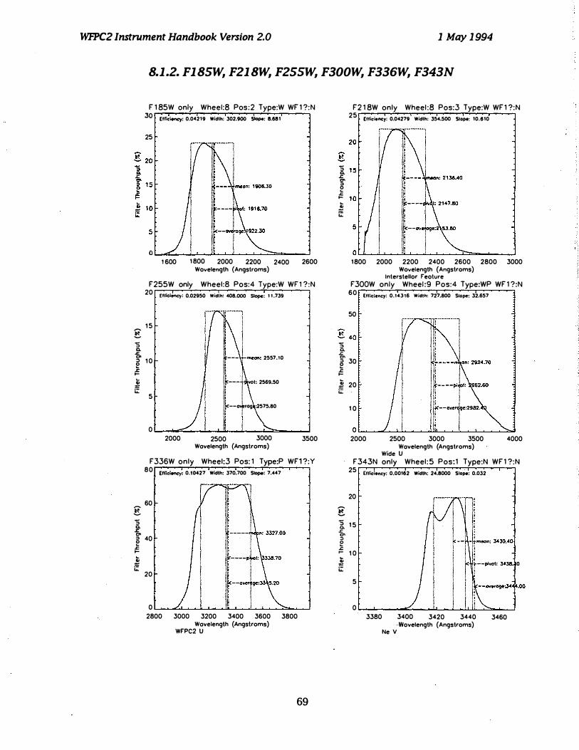
WFPC2 Instrument Handbook Version 2.0 1 May 1 994
8.1.2. F185W, F21 8W, F25SW, F300W, F336W, F343N
...... � "5 Co .s:: '" " e .s:: I-� �
g "5 Co .r; '" " e .s:: I-.. ., "" �
F 1 85W only Wheel:8 Pos:2 Type:W WF 1 ?:N 30 Effie;..,q.: 0.04219 Width: 302.900 Slope: 8.681
25
1 600 1800 2000 2200 2400 Wovelength (Angstroms)
2600
F255W only Wheel:8 Pos:4 Type:W WF 1 ?:N 20 EffiCiency: 0.02950 Width: 40S.OOO stope: 1 1 .739
1 5
10
5
0 2000
�-l :. : ij::--- :-mean: 2557.10 :) . OJ OJ OJ " !�---� ·vot: 2569.50 II I 1:<--"""'09 :2575.S0 !� i II I
2500 3000 Wovelength (Angstroms)
3500
F336W only Wheel:3 Pos: 1 Type:P WF1 ?:Y 80 Ellieioney: 0.100427 Width: 370.700 Slope: 7.447
60
40
20
0 2800 3000 3200 3400 3600 3800
Wovelength (Angstroms) wrpC2 U
69
"5 c. .r; '" " o � .. � �
"5 Co .s:: '" " e .r; I-
� �
E "5 c. .s: '" " e .c I-t "" �
F2 1 8W only Wheel :8 Pos:3 Type:W WF 1 ?:N 25
Efficioncy: 0.04279 Width: 354.500 Slape: 10.1110
1800 2000 2200 2400 2600 2800 3000 Wovelength (Angstroms)
Interstellor reoture F300W only Wheel :9 Pos:4 Type:WP WF 1 ?:N
60 Efficiency: 0.143'6 Width: 727.S00 SlOpe: 32.657
50
30
20
1 0
o ��������������� 2000 2500 3000 3500 4000
Wovelength (Angstroms) Wide U
F343N only Wheel : 5 Pos:1 Type:N WF 1 ?:N 25 Effieiency: 0.00162 Width: 24.8000 Stope: 0.032
20
1 5
1 0
5
0 3380 3400 3420 3440
Wovelength (Angstroms) Ne V
3460
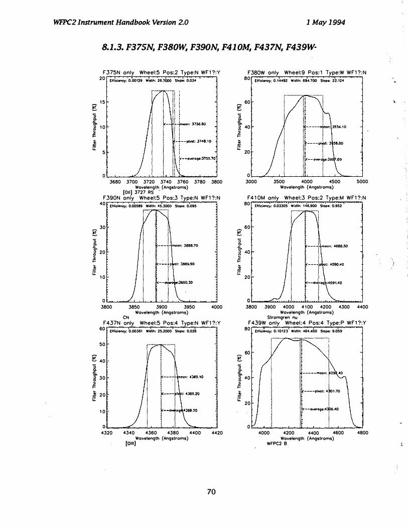
WfPC2 Instrument Handbook Version 2.0 1 May 1 994
8.1.3. F37SN, F380W, F390N, F41 0M, F437N, F439W·
.... e :; a. .::: D' ::> e .::: l-t
"'" �
.... e :; a. .::: '" ::> e
.::: I-
� �
....
F375N only Wheel:5 Pos:2 Type:N WF 1 ?:Y 20 Effici.ncy: 0.00139 W;,tlh: 26.7000 Slope: 0.034
1 5
1 0
5
3680 3700 3720 3740 3760 3780 3800 Wovelength (Angstroms)
[OU] 3727 RS -F390N only Wheel:5 Pos:3 Type:N WFl ?:N
40 Effici.ncy: 0.00589 Wth: 45.3000 Slope: 0.095
30
20
1 0
0 3800
� ····· .. 1
i � t---i meon: 3888.70
· , · , · , · ,
r:r-" g ! · , :) :
3850 3900 3950 4000 Wovelength (Angstroms)
CN F437N only Wheel:5 Pos:4 Type:N WF1 ?:Y
60 Efficiency: 0.00361 Wth: 25.2000 Slope: 0.026
50
� 40 :;
, , , , , , , , ! ! a. .::: D' � 30
� I-... .! 20 iZ
, . f----i , , , , , , 1 � 1<:----;, : ! , : , : , : , :
1 0 k--�o
O L-____ -=� ____ �� __ ,�; ���I ____ �� ____ �
4320 4340 4360 4380 4400 Wovelength (Angstroms) [0111]
4420
70
.... e :; a. .::: D' ::> 0 ..c I-... ., "'" �
.... e :; a. .::: D' ::> 0 ..c I-... � �
F380W only Wheel:9 Pos: 1 Type:W WF1 ?:N 80 Effici.ncy: 0.1"92 W;dth: 69'.700 Slope: 22.124
60
40
20
0 3000 3500 4000 4500 5000
Wovelength (Angstroms)
F4 1 0M only Wheel:3 Pos:2 Type:M WF1 ?:N 80 Efficiency: 0.03305 W;dth: 1 46.900 Slope: 0.952
60
20
I I I I I i i �---I I I
t----ic--�rag :4091.40 I i o � __ ���������� ____ �
3800 3900 4000 4 1 00 4200 4300 4400 Wovelength (Angstroms)
Stromgren nu F439W only Wheel : 4 Pos:4 Type: P WFl ?:Y
80 Efficiency: 0.10123 Width: 464.400 Slope: 9.059
60
40
20
0 4000 4200
" g II !� �------< l� " iif'----pNot: 4lKl1 •70 I� I l1,c--overoge:4J/J6.40 l� I
4400 4600 Wovelength (Angstroms)
WFPC2 B
4800

WF.PC2 Instrument Handbook Version 2.0 1 May 1994
8.1.4. F4S0W, F467M, F469N, F487N, FS02N, FS47M
E 'S Q. ..0:: '" ::> !:l ..0:: ...
� �
'S Q. ..0:: '"
F4S0W only Wheel : 1 0 Pos:4 Type:WP WF 1 ?: N 100
EW"*"'r: 0.2472. W'odlh: 025.000 Slop.: �.711
80
60
40
20
4000 4500 5000 Wavelength (Angstroms)
Wide B
5500
F469N only Wheel:6 Pos: 1 Type:N WF 1 ?:Y 80 Effici .... Y' 0.00.03 Widlh: 24.9000 Slope: 0.024
60 . .
� 40 i k-----� : 4694.50 1:
.... ... � E
E 'S Q. ..0:: '" ::> !:l ..0:: .... II f:
20
i ! �----piv4t: .. 94.40 I i I i k--aver�:469 I I O ����� __ ������� __ �
4660 4670 4680 4690 4700 471 0 4720 4730 Wavelength (Angstroms)
He II FS02N only Wheel:6 Pos:3 Type:N WF1 ?:Y
80 Efficiencr: 0.00413 W'odlh: 26.9000 Slope: 0.026
60
40
20
0 4980 4990 5000 5010 5020 5030 5040 5050
Wavelength (Angstroms) (0111)
71
F467M only Wheel :3 Pos: 3 Type:M WF 1 ?:N 100 Elneio"cr: 0.03796 W'odlh: 171 .• 00 Slo�: 1 .132
80
1 60 ..0:: '" ::> . !:l ..0:: .... 40 � l:
20
O � __ �-d��������� __ � 4300 4400 4500 4600 4700 4800 4900 5000
Wavelength (Angstroms) Stromgren b
F487N only Wheel :6 Pos:2 Type:N WF 1 ?:Y 80 EfOci,"cr: 0.00.38 W'odlh: 25.8000 Slope: 0.025
4820 4840 4860 4880 4900 Wavelength (Angstroms)
H beta FS47M only Wheel :3 Pos:4 Type:M WFl ?:Y
1 00 EWeie"cr: 0.10.36 'Mdlh: .86.600 Slope: 7.828
80
1 60 ..0:: '" ::> !:l ..0:: .... 40 ... '" :: �
20
5000 5200 5400 5600 Wovelen9th (Angstroms)
Stromgren y (but wider)
5800 6000
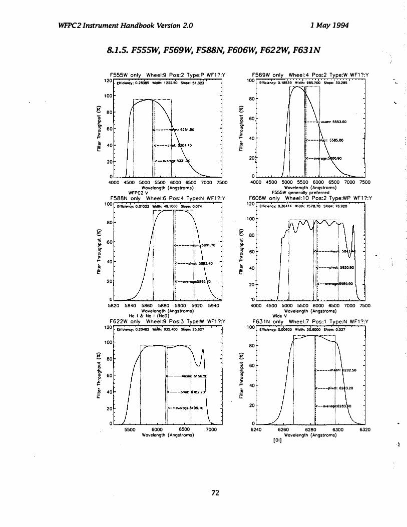
WfPC2 Instrument Handbook Version 2.0 1 May 1994
8.1.5. F55SW, F569W, F588N, F606W, F622W, F631N
......
� :; Q. L "" " 0 .c ...
� :0: i:
......
� :; Q. L "" " e L ...
� i:
g :; Q. L "" " 0 .E
...
] i:
F555W only Wheel:9 Pos:2 Type:P WF1 ?:Y 1 20 Effi ..... cy: 0.28311S WIdth: t222.50 SIOp4f: 5' .323
1 00
80
60
40
20
0
iI! i I· I II I ,· " ". ' " \ 1. I I I : I'
ff-----
ILl-"" . I ii I 4000 4500 5000 5500 6000 6500 7000 7500
Wavelength (Angstroms) wrpC2 V
F588N only Wheel:6 Pos:4 Type:N WF1 ?:Y 1 00 Effic;oncy: 0.0'022 Wodth: �9.'OOO Slop4f: 0.07�
80
60
40
20
n 1 1 n n i : 1 : " " " " : a . 14-----m.on: 5891 .70 n ! : a : i I ! !k----piv�t: 58 3 •• 0 H � U ! ! I<" --overog.:589J. 0 II I O � __ ����-J __ �������
5820 5840 5860 5880 5900 5920 5940 Wavelength (Angstroms)
He I & Na I (NoD) F622W only Wheel:9 Pos:3 Type:W WFl ?:Y
120 Efficiency: 0.20�82 Wodth: 93S.�00 Slope: 25.627
100
80
60
40
20
0 5500 6000 6500
Wavelength (Angstroms) 7000
72
......
� -" Q. L "" " 0 .c
...
�
� i:
...... � :; Q. L "" " e J:
...
� i:
......
� :; Q. L "" " 0 .E ...
] i:
F569W only Wheel :4 Pos:2 Type:W WF1 ?:Y 100 [frociency: 0.'8539 Width: 18S.7oo SIopo: 30.28S
80
60
40
20
0
··"ff· .. ······!
i) J I, j h . !� ,I. 1: 11 : �--- 1m.on: 5553.60
" " !�----�. 1� � !: ! i:< --overage: II I
4000 4500 5000 5500 6000 6500 7000 7500 Wavelength (Angstroms)
r555W generally preferred F606W only Wheel: 1 0 Pos:2 Type:WP WF 1 ?:Y
120 Efroeiency: O.36� '4 Width: 1578.70 Slope: 76.920
1 00
80
60
40
20
0 4000 4500
···T:;····
1i I I! I I! �.i.----meo�: 58 3
i i! I ! �----pivot! 5920.90 i ii i � �i ! ! ii<--..-ogei5959.9O I II I
5000 5500 6000 6500 7000 7500 Wavelength (Angstroms)
Wide V F63 1 N only Wheel :7 Pos : 1 Type:N WF1 ?:Y
1 00 Emciency: 0.00603 Width: 30.6000 Slope: 0.027
80
60
40
20
0 6240
it if if !r " " if 1: " I-----mr !1<----piva1: 62 3.20 II I !:C--overogf:6283. 0 !! !
6260 6280 6300 Wavelength (Angstroms)
[01)
6320
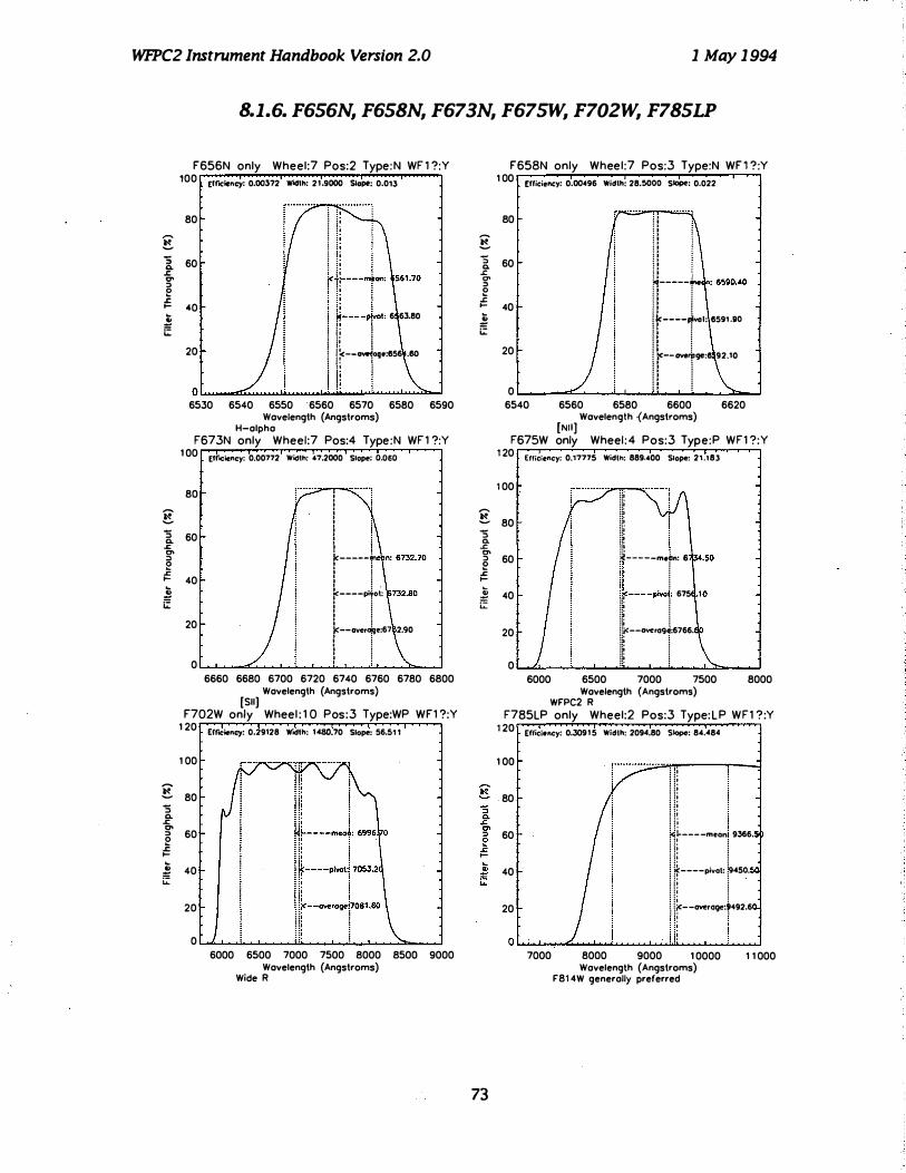
WfPC2 Instrument Handbook Version 2.0 1 May 1 994
8.1.6. F656N, F658N, F673N, F675W, F702W, F785LP
,... � "'5 Q. J:. '" :> !? J:. I-� E
g "'5 Q. .r; '" " !? .r; I-� .! �
..... � "'5 Q. J:. '" " !? J:. I-� � i:
F656N only Wheel:7 Pos:2 Type: N WF 1 ?:Y 100 EffICiency: 0.00372 WlIlIh: 21.9000 Slope: 0.013
80
60
40
20
I ! ! i : l . nr---Tn: ! H----p!-ol: 6 63.80
i i i ! I Ii i i 11�--�9.:656 .60
i I f ! I I ' I I I I 1 o � __ ������������� 6530 6540 6550 6560 6570 6580 6590
Wavelength (Angstroms) H-alpha
F673N only Wheel:7 Pos:4 Type:N WF 1 ?:Y 1 00 EffICiency: 0.00772 W�lh: 07.2000 Slope: O.OBO
80
60
40
20
0
· l l l I I
I \ r-----t I , I , I : . �----piTot: · , I , I , I , · , I , !<--..... "!'ie:67 I , · , I , · , I , I 1
2.90
6660 6680 6700 6720 6740 6760 6780 6800 Wavelength (Angstroms)
[Sll) F702W only Wheel : 1 0 Pos:3 Type:WP WF1 ?:Y
1 20 EffICiency: 0.29128 WocIth: 1460.70 Slope: 56.511
1 00
80
60
40
20
0 6000 6500 7000 7500 8000 8500 9000
Wavelength (Angstroms) Wide R
,... � "'5 Co J:. 0' " !? J:. I-
� i:
..... � "'5 Q. .r; '" " !? .r; l-
� i:
73
F658N only Wheel:7 Pos:3 Type:N WF 1 ?:Y 1 00 Efficiency: 0.00496 Widlh: 28.!IOOO Slope: 0.022
80
60
40
20
0
; . n " " n n " " n " �-----r i k----�I: 659UO I i I i :<--.... .;,9":6 92.10 I i I
6540 6560 6580 6600 6620
[Nil) Wavelength {Angstroms)
F675W only Wheel : 4 Pos:3 Type:P WF1 ?:Y 1 20 EWciency: 0.17775 Width: 889.'00 Slope: 21.183
1 00
80
60
40
20
0
::. " ::. " :: . " ::. " ::-" i� i� ::. ii!-----mei.n: 6 Ii I ioc----piva{: 675 Ii I iil<--over094,6766. I! I
6000 6500 7000 7500 8000 Wavelength (Angstroms)
WFPC2 R F785LP only Wheel:2 Pos:3 Type: L P WF1 ?:Y
1 20 Efficiency: 0.30915 Width: 2094.80 Slope: 84.484
1 00
80
60
40
20
r··········::.:;····""··· ... · ...... ---..,...-..:::J I I II Hi i ii
Ul----meani 9366. l H ! I �----Pivat: �4SO.
1 1�--over09":�.92.6 I i i 1 o ���������������� 7000 8000 9000 1 0000
Wavelength (Angstroms) F81 4W generally preferred
1 1 000

WFPC2 Instrument Handbook Version 2.0 1 May 1 994
8.1.7. F791 W, F814W, F850LP, F953N, F1 042M, FQUVN-A
�
F79 1 W only Wheel:4 Pos: 1 Type:WP WF 1 ?:Y 1 20 Elfieioftcy. 0.2246' Width: 130 •. 20 510p0: 38.3"
1 00
� 80
"S Q. .c .,.. " 60 e .c .... .. � 40 j;:
�
� "S Q. .c .,.. " 0 1: ....
� j;:
g -::> Q. .c .,.. ::> e .c .... .. � j;:
20
7000 SOOO 9000 1 0000
Wavelength (Angstrams) rS14W generally preferred
1 1 000
F850LP only Wheel:2 Pos:4 Type:LP WF1 ?:Y 1 00 Effici.ncy. 0.23369 WIdth: 1669.50 Slo e: 51 .805
f··n..... l li 80
60
40
I Ii : 11 i ii Hi : �i----meon: �702.70 I ii I i it----pivot: 9711 •.• 0 I Ii I i i!<--owrage:9780.30
o � __ ����������I�ll __ � __ ��I� __ �
20
SOOO 8500 9000 9500 1 0000 1 0500 1 1 000
Wavelength (Angstroms)
F 1 042M only Wheel : 1 1 Pos:2 Type:M WF1 ?:Y 1 20 Efficiency. 0.07772 Width: 610.900 Slopo: 6.445
1 00
SO
60
40
20
0
9800
�
I t------: �10.43.
I I iIc----p;"O,: ' •• 50.0 I I ik--overage:l0�53.2 I !
10000 1 0200 1 0400 1 0600 1 0800 1 1 000
Wavelength (Angstroms)
� � "S Q. .c .,.. ::> e .c .... .. � �
g "S Q. .c .,.. ::> 0 1: ....
� j;:
F8 1 4W only Wheel : 1 0 Pos: 1 Type:P WF1 ?:Y 1 20 Efficiency: 0.:19744 Width: '7�.00 $lope: 87.402
1 00
80
60
40
20
0
7000 SOOO
HI I I !,ii-----mei.n: 112 9.'0 H� ! !�----pi�: 833 I ii ! i ii<--overog�:8370. I!i I
9000 1 0000 1 1 000
Wavelength (Angstroms) WrpC2 I
F953N only Wheel: 1 Pos: 1 Type:N WFl ?:N 1 00
Efficiency: 0.00674 Width: 54.5000 Slope: 0.056
80
60
40
20
0
9450 9500 9550 9600 9650
Wavelength (Angstroms) [Sill)
FOUVN-A only Wheel: 1 1 Pos:3 Type:O WF 1 ?:N 3 0 Efficiency: 0.00!598 Width: 73.4000 Slape: O.2�
25
5
I i I k-----moi.n: 3765.80 i l k----pivo,j 37 5.60 I , I l I , I : �--ove,age:�765 I , I , I , I ,
O �� __ � ____ � __ ���I� ____ �i ____ ��--" 3700 3750 3800
Wavelength (Angstroms) Redshifted [011) 375
3850
74

WfPC2 Instrument Handbook Version 2.0 1 May 1 994
B.l.B. FQUVN-B, C and D, FQCH4N-A, B and C
FQUVN - B only Wheel : 1 1 Pos:3 Type:Q WF 1 ?:N 40 EfflClellCy. D.�5 Wldlh: 57.4000 Slope: D.155
E :; Q. .&. '" " � .&. ... .. � r;:
30
20
1 0
0
I -----m .. n: 3831.10
i ----pivoli ; ! --ov.ro;.:�83O.
! !
3760 3780 3800 3820 3840 3860 3880 3900 Wovelength (Angstroms)
Redshifted [011) 383 FQUVN- D only Wheel : 1 1 Pos:3 Type:Q WF1 ?:N 50 Eff",iellCy. D.00873 Wldlh: 63.6000 Slope: o. '83
40
1 0
: i ! i k-----..iea I i ! ! �----p;.J,: 3 92.80 I I :<,--averag�:399 .80 , , , , , , , , , ,
0 �� __ ��� __ �:� ____ �1� __ -L� __ ��--J 3950 4000 4050 4100
Wovelength (Angstroms) Redshifted [011] 399
FQCH4N - 8 only Wheel : 1 1 Pos:4 Type:O WF1 ?:N
g -" Q. .&. "" " e .&. ... � r;:
100 Eff",iellCy. 0.00617 Wldlh: 157.700 Slope: 0.716
80
60
40
20
0 6100
) 6150 6200 6250 6300
Wovelength (Angstroms) CH4 619
g :; Q. .&. '" " e .&. ... � :t::
r;:
FQUVN -C only Wheel: 1 1 Pos:3 Type:O WF 1 ?: N 50 Elfltlency: 0.00755 Wldlh: 5Q.JOOO Slope: D.182
40
10
1: 1; a " " " �-----+n
1�----p;.J,: 3 14.50 II I ;",--.-,,*:391
0 L-��� __ � __ ��!�:1� ____ �1-L ____ �� __ -J 3850 3900 3950 4000
Wovelength (Angstroms) Redshifted [011) 39 1
FOCH4N-A only Wheel : 1 1 Pos:4 Type:O WF 1 ?:N 1 00 Efficiency: 0.00677 Wld,h: 72.3000 Slope: 0.'72
80
60
40
20
0
,\r l l I ! I i ! i<---i--fmeon: 5462.30
I I i I I I r-t--pivol: 5485.00
l i ! ! ! ! 1<--... .,og.:5498.70 ) i �,. i i l l\ l ! 5350 5400 5450 5500 5550 5600
Wovelength (Angstroms) CH4 543
FOCH4N-C only Wheel: 1 1 Pos:4 Type:O WF 1 ?:N 1 00 Efficiency: 0.00624 Wldlh: 1 12.400 Slope: 0.31 1
7200
75
7250 7300 7350 Wovelength (Angstroms)
CH4 727
7400

WfPC2 Instrument Handbook Version 2.0 1 May 1994
8.1.9. FQCH4N-D, -Parallel and Perpendicular Polarizers
� � :; Q. .<: '" :> � .<: .....
� iZ
FOCH4N - D only Wheel: 1 1 Pos:4 Type:O WF1 ?:N 1 00 Efl;cloncy. 0.0071 7 _IeII.: 811.2000 Slope: 0.094
80
20
O bc __ -=�������� ____ � 8800 8850 8900 8950 9000 9050
Wavelength (Angstroms) CH4 892
POLO_per only Wheel: 1 1 Pas: 1 Type: WF1 ?:N 1 00 EII;cIoncy. 0.34663 Yfodl.: 6653.40 Slope: 1007.753
80
60
40
20
0 2000
r········· .. ·················'· .. ···rT················ .
I I i i : ! I
4000 6000 8000 1 0000 Wavelength (Angstroms)
0.45,90,135
.10
76
�
� ;; Q. .<: '" '" � .<: ....
� iZ
POLO_par only Wheel : 1 1 Pos : 1 Type: WF 1 ?:N 1 00 Elroclency. 1 .00517 ""dl.: 5797.60 Slope: " 16.892
80
60
, ........ · ............ · .. '[" .... ·r .. r .... ·· . . ·1
I r---i-t�r .. ; !<-�--pOwoll &498.70
I I r--+-'" O �� __ -L __ ����A-�� __ �� __ �
2000 4000 6000 8000 Wovelength (Angstroms)
0,45,90,1 35
1 0000

WFPC2 Instrument Handbook Version 2.0 1 May 1 994
S.2. PASSBANDS INCLUDING TIfE SYSTEM REsPONSE
8.2.1. F122M, F130LP, F1 60AW, F1 60BW, F1 65LP, F1 70W
0.040
F 1 22M Wheel : 1 Pes:4 Type:M WF 1 ?:Y
EIIld.ncy. o.� Wldlh: 850.Il00 Slope: 103." 5
�Q.' 0.030
�!:, ...... ··· .. ·· .. · .. · .. l· .... ··· .. · ........ · .... , - i f � I i i , :" . fC-----meoft: 1S$1.50 !
E ..
i III 0.0 1 0
1 000 1 200 1 400 1 600 1800 2000 2200 2400
Wavelength (Angstroms)
0.08
E 0.06
:> Q.
..r: tI' :> � 0.04
....
E ..
i III 0.02
H Ly alpha - Red Leak F 1 60AW Wheel: 1 Pes:} Type:W WF 1 ?:N
Elrtc:ioncy. 0.00025 W"odlh: �2.2oo Slope: 33.333
0.00 ........ �.u...... ............... � ....... � ........ :.........-..L-�-'-.....:: __ -..J
� e. 'S Q. ..r: tI' :> e ..r: ....
E ..
iii .... III
1 000 1 200 1 400 1 600 1 800 2000 2200 2400
Wavelength (Angstroms)
1 5
1 0
5
Woods A - redleak from pinholes F 1 65LP Wheel:2 Pes:2 Type:LP WF1 ?:N
2000 4000 6000 8000
Wavelength (Angstroms) Suprasil Blocker (zero focus)
1 0000
1 5
� t:.. 'S 1 0
Q. ..r: tI' :> e ..r: ....
2198.70 � iii rtI
5
<--overo
0.08
E 0.06
'S c. ..r: tI' :> o 0.04
� E .! VI ....
III 0.02
F 1 30LP Wheel:2 Pes : 1 Type:LP WF 1 ?:N
2000 4000 6000 8000 1 0000
Wavelength (Angstroms) CaF2 Blocker (zero focus)
F1 60BW Wheel: 1 Pes:2 Type:W WF1 ?:N Elfic:ionc:y; 0.00025 W"odlh: 542.200 Slop.: 33.333
r·············T-!·l······· � 1 H 1 1 :; i Hi
: a . �"t----� n: 1 590.70
! ll ! : : . : ! �----pi�o': ' 625.00 I I! ! i ii<--ov ... +¥:164 .50 I II I 0.00 ........ �.u.........:... ........ � ....... � ........ �-..L-� ......... .....;::,.".. -.J
1 000 1200 1 400 1 600 1 800 2000 2200 2400
Wavelength (Angstroms) Woods B
F 1 70W Wheel:8 Pes : 1 Type:W WF1 ?:N 0.20
Elfic:ionc:y: 0.00046 W"od,h: 526.300 Slo�: 27.537
E 0. 1 5
1 ..r: tI' :> e 0. 1 0 ..r: .... E ., Ui ....
III 0.05
77
0.00 1G.....:.......�l....L�.....L..J...i. ......... L...... ........ ........JL::::;:::::I::;::j 1 200 1 400 1 600 1 800 2000 2200 2400 2600
Wavelength (Angstroms)
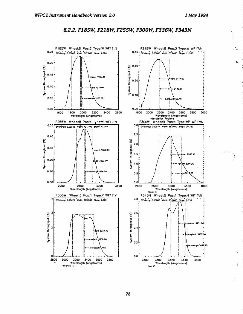
WfPC2 Instrument Handbook Version 2.0 1 May 1994
B.2.2. FIB5W, F21BW, F255W, F300W, F336W, F343N
0.25
0.20 E -; 0. 0. 1 5 t. " !! .l! l-E 0. 1 0 � .. JI
o.os
F 1 B5W Wheel:B Pos:2 Type:W WF 1 ?: N
[.rod.n"y: 0.00042 Wldlh: 317.000 Slope: 9.278
0.00 L.......::::::""""......JL...._i..li.J..._.L..........I-_--===='
�
� -;
1 600 1 800 2000 2200 2400 2600 Wavelength (Angstroms)
F255W Wheel:B Pos:4 Type:W WF1 ?:N 0.SO r-E�w�-·�en-"-y�: 0-.���--�WI-,dTlh-:�4-2-1.�7oo�-Sl�0�pe-r: -12�.2-8�9--���
0.40
.f 0.30 '" " !! � E 0.20 II iii JI
0. 1 0
0.00 L.....o ........ _:::....._....i..--'-........ �..l--.....J'---"= __ ...J
g -" <>-.J:: '" " � .J:: l-E II iii >. en
2000
F336W
2500 3000 3500 Wavelength (Angstroms)
Wheel:3 Pos: 1 Type:P WF1 ?:Y 4 Elrodency: 0.00425 WIdth: 379.700 Slope: 7.829
3
2
3000 3200 3400 3600 Wavelength (Angstroms)
WFPC2 U 3800
0.40
E 0.30
-; 0. t. " !! 0.20 .l! ... E to iii >. en 0 . 1 0
F2 1 BW Wheel:B Pos:3 Type:W WF1 ?: N
Elli<;.ooy: o.oooee Wldlh: 373.400 Slope: 1 1.585 ........... ,
! I ;neon: 2174.00
1 800 2000 2200 2400 2600 2800 3000 Wavelength (Angstroms)
Interstellar Feature F300W Wheel:9 Pes:4 Type:WP WF1 ?:N
3.0 Elroc;eooy: 0.00577 WIdth: 682.900 Slope: 28.380
2.5
g :; 2.0 0. .J:: '" "
1 .S 0 ..c l-E � III 1 .0 >. en
o.s
0.0 2000 2500 3000 3500 4000
0.8
g 0.6
-; 0. .l! '" " e 0.4 .J:: .... E .. iii >. en 0.2
Wavelength (Angstroms) Wide U
F343N Wheel:5 Pes: 1 Type:N W F 1 ?:N
Elrodency: 0.00006 WIdth: 2r=�.1lQ9 •• S1!!nr34
i i i i n +�ml!an: 3431.2 i i i i i !
k ·f--p;wt: 3437.
! I 0.0 '----'-__ """"'��'-'-L_....:..........:..J ........ ........;""., ..... ....J
78
3380 3400 3420 3440 Wavelength (Angstroms)
Ne V
3460

WfPC2 Instrument Handbook Version 2.0 1 May 1994
8.2.3. F375N, F380W, F390N, F410M, F437N, F439W
1 .0
0.8 --� '5
"- 0.6 .s: .,. ::J 0 l:
.... E 0.4 � .. >. (II
0.2
0.0
2.0
E 1 .5
'5 ".s: '" ::J !? 1 .0 .s: .... E '" tii >. (II 0.5
3.0
2.5
g '5 2.0 Q. .s:: '" ::J !? 1 .5 � E .! 1 .0 .. .:0
0.5
F375N Wheel:5 Pos:2 Type:N WF 1 ?:Y
Efficiency: 0.00008 Widlh: 26.7000 Slope: 0.0301
3680 3700 3720 3740 3760 3780 3800 Wovelength (Angstroms)
[Oil] 3727 RS F390N Wheel:5 Pos:3 Type:N WF 1 ?:N
Ellicioney: 0.00029 Widlh: 45.3000 Slope: 0.095
mean: 3888.70
I: 3889.50
3850 3900 3950 Wovelength (Angstroms)
CN
4000
F437N Wheel:5 POS:4 Type:N WF 1 ?:Y
Elliciency: 0.00019 Widlh: 25.2000 Slope: 0.026
, ,
I :<----r-, , , : , : , : , : : 1 . I<----p , : , : , : , : , : , : , : j<--ovet09 , : , : , : , : , : , : O.O L-____ -=�������' ���; ���=_ ____ �
4320 4340 4360 4380 4400 Wovelength (Angstroms)
[0111] 4420
79
E '5 "-.s: .,. ::J 0 l: ....
E " tii >. (II
--� '5 Q. .s:: '" ::J !? .s:: ....
E '" tii >. (II
'5 Q. .s:: '" ::J
F380W Wheel :9 Pos: 1 Type:W WF 1 ?:N 4
Efficiency: 0.00707 Yndlh: 080.100 Slope: 21.032
3
2
o ���������������� 3000 3500 4000 4500 5000
Wovelength (Angstroms)
F4 1 0M Wheel :3 Pos:2 Type:M WF1 ?:N 5
Efficiency: 0.00175 Yndlh: 146.500 Slope: 0.946
4
3
2
, , l i I i , : t---� . : , : , : , : , : k---"'; , : , : , : , : , : t--ov�ro
O ���������������� 3800 3900 4000 4 1 00 4200 4300 4400
Wavelength (Angstroms)
4
Stromgren nu F 439W Wheel :4 Pos:4 Type:P WF1 ?:Y
EfficiencY: .. Q,9!!�54 •• "Y!!!��:. �?'�:;!Q9 ... ?I!!�; 9.437
I II I l� �-----meon: �303. 10
e 2 It. I .s:: .... E '" tii >. (II
ii!"----pivol: 4j12.70 II I ir=--overOCJe:43� 7.60
O L-���������II�� __ ��:�;� __ ����
4000 4200 4400 4600 Wavelength (Angstroms)
WFPC2 B
4800

WH'C2 Instrument Handbook Version 2.0 1 May 1994
8.2.4. F4S0W, F467M, F469N, F487N, FS02N, FS47M
--!!. 'S Q. �
F450W Wheel : 1 0 Pos:4 Type:WP WF1 ?: N 1 0 Elliclency: 0.01559 W'odth: 951.400 Slope: 36.059
3500 4000 4500 5000 5500 Wavelength (Angstroms)
Wide B F469N Wheel:6 Pos: 1 Type:N WF 1 ?:Y
5 Efficiency: 0.00027 W'odth: 24.9000 Slope: 0.024
4
3
· · · · · · · : '" ! " e � l-E QI 1ii >. VI
--� 'S Q. � '" " e � l-E .!
UI
Ji'
2
k-----rrieo : 4694.40 · , · , · , · , · , · , k- ---pivqt: .. 94.40 I : · , · , · , · , r--�r09r:469 · , I !
O ����������:����! ���� __ � 4660 4670 4680 4690 4700 47 1 0 4720 4730
Wavelength (Angstroms) He II
F502N Wheel : 6 Pos:3 Type:N WF1 ?:Y 6
Efficiency: 0.00036 W'odlh: 26.9000 Slope: 0.026
5
4
3
2
I : : �-----m�n: 5012.80 · , · , · , · , i i �----p;yol: 50 3.10 · , · , · , · , � 1 · , r--ovet'0CJ4f:5013. · , · , · , : !
O ����������·����;����� __ � 4980 4990 5000 50 1 0 5020 5030 5040 5050
Wovelength (Angstroms) (0111)
E
F467M Wheel :3 Pos: 3 Type:M WF 1 ? : N
6 Elliclency: 0.00248 Widlh: 186.300 SlOpe: I .oee ! ........ T ....
I i
.! 2 �::l��,::·� II> >. VI
--!!. 'S 0-� '" " e � l-E QI 1ii >. VI
--!!. 'S Q. � '" " e � l-E QI 1ii >. VI
80
r--i : 1 o ��� __ ���������� __ � 4300 4400 4500 4600 4700 4800 4900 5000
Wavelength (Angstroms) Stromgren b
F487N Wheel : 6 Pos:2 Type:N WFl ?:Y
6 EWci.ncy: 0.00034 Width: 25.8000 Siopo: 0.025
5
4
3
2
" " " " " " " " " " " " " " �-----�e n: 4865.00 Ii .I ,i<----poyot: !i i il<--ove,qge:48 5.70 !i I O ����������������
4820 4840 4860 4880 4900 Wavelength (Angstroms)
H beta F547M Wheel : 3 Pos:4 Type:M WF1 ? :Y
1 2 Elfociency: 0.01223 Width: 486.100 Slope: 7.779
1 0
8
6
4
2
0 5000 5200 5400 5600 5800
Wavelen9th (Angstroms) Slramgren y (but wider)
6000
, ..

WFPC2 Instrument Handbook Version 2.0 1 May 1994
8.2.5. F555W, F569W, F588N, F606W, F622W, F631N
E 4> iii ?>
g
F555W Wheel:9 Pes:2 Type:P WF l ?:Y 1 2 Elncioney: 0.029 1 0 Width: 1231.60 Slape: 50.668
1 0
8
6
4
2
o ������������--� 4000 4500 5000 5500 6000 6500 7000 7500
Wavelength (Angstroms) WF'PC2 V
F588N Wheel:6 Pes:4 Type:N WF1 ?:Y 15
Ellicioney: 0.00146 Wldlh: 49.0000 Slape: 0.073
5820 5840 5860 5880 5900 5920 5940 Wavelength (Angstroms)
He I & No I (NoD) F622W Wheel:9 Pes:3 Type:W WFl ?:Y
15
:; 10 Q. � 0-" o .E .... E ., 5 ].
5500 6000 6500 Wavelength (Angstroms)
7000
:; Q. .J: '" "
F569W Wheel:4 Pes:2 Type:W WF l ?:Y 12 Ellicieney: 0.02221 Width: 968.900 Slape: 30.134
1 0
8
6
4
2
o ��������������� 4000 4500 5000 5500 6000 6500 7000 7500
Wavelength (Angstroms) F'555W generally preferred
F606W Wheel: 1 0 Pes:2 Type:WP W F l ?:Y 20 Efficieney: 0.04485 Width: 1500.1 0 Slape: 68.322
o 1 0 � E II> 1 Vl 5
E
4000 4500 5000 5500 6000 6500 7000 7500 Wavelength (Angstroms)
Wide V F63 1 N Wheel:7 Pes: 1 Type:N WF1 ?:Y
15 Efficieney: 0.00087 Width: 30.7000 Slope: 0.027
:·······�··--,..l-..:.:: I
! I I :;
1 0 Q.
; ! .J: '" " e .J: ....
8 1
5
I k-----m�n: I : � i : ! I : I : !<----p""l: 62 I : , : � i , : , : k--'-D<l<i:6282. i ! I i ; !
O � __ cC� __ ��� ____ �' __ � __ �;� ____ �� 6240 6260 6280 6300
Wavelength (Angstroms) [01]
6320
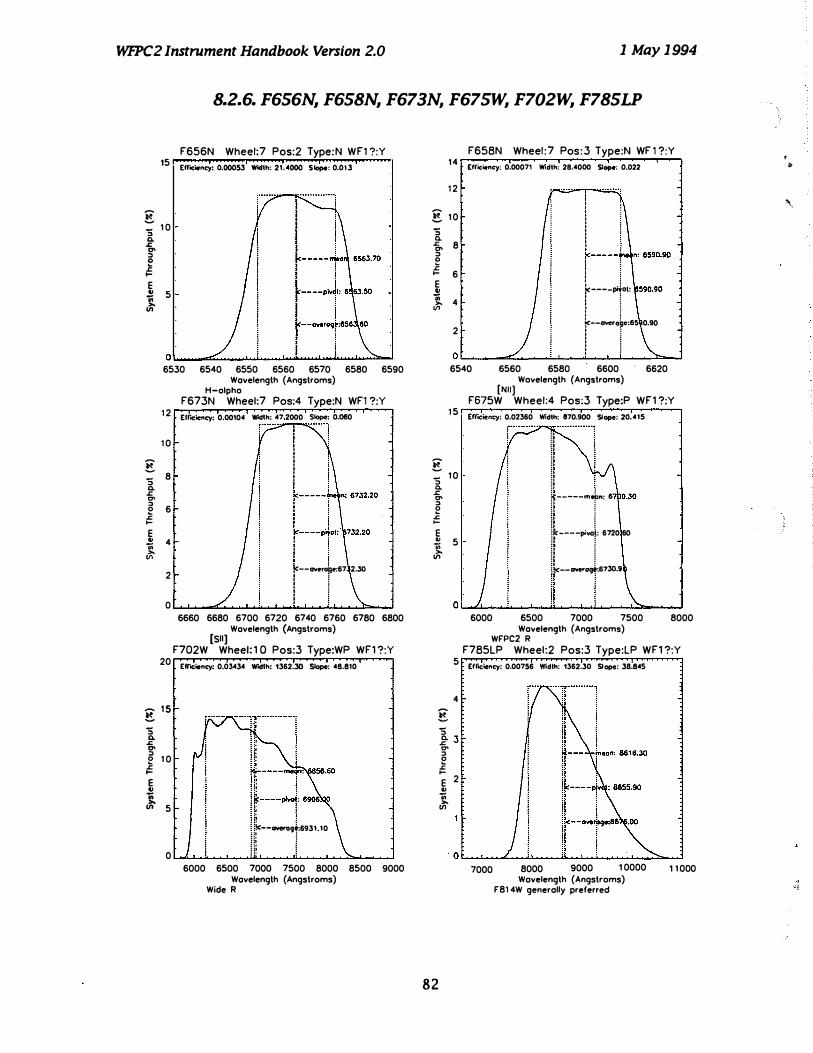
Wfl'C2 Instrument Handbook Version 2.0 1 May 1 994
8.2.6. F656N, F658N, F673N, F675W, F702W, F785LP
g
F656N Wheel:7 Pos:2 Type: N WFl ?:Y 15
Efflc:iency: 0.00053 W'ldth: 21.4000 Slope: 0.013
"5 1 0 0-.t:. '" ::> o � E " 5 £
�
� "5 0-.t:. '" ::I e .t:. l-E .!! .. >. II>
E "5 0-.t:. '" ::> e .t:. l-E " 0; >. II>
o � __ ������������� 6530 6540 6550 6560 6570 6580 6590
1 2
1 0
8
6
4
2
0
Wavelength (Angstroms) H-olpho
F673N Wheel:7 Pos:4 Type:N WF1 ?:Y
Emeiency: 0.00104 W'tdlh: 47.2000 Slope: 0.060 : ! I : : : I
r::::l t<--overoae:67 i ! i i
2.30
6660 6680 6700 6720 6740 6760 6780 6800 Wavelength (Angstroms)
[SII) F702W Wheel: 1 0 Pos:3 Type:WP WF1 ?:Y
20 Eff'lCiency: 0.03434 W'tdlh: 1362.30 Slope: 4S.S10
1 5
1 0
5
0
<r " 1 : :1 :
F-1-l lic--overag.:6931.10 !� ! i � i
6000 6500 7000 7500 8000 8500 9000 Wavelength (Angstroms)
Wide R
F658N Wheel : 7 Pos: 3 Type:N WF l ?:Y 14
E"-=ioncy: 0.00071 Wodth: 28.4000 SI_: 0.022
1 2
g 10 "5 0-f" 8 ::> o .J: I- 6 E .!!
� 4
2
i : : I r-----i I , I , r----101: I , I , , , I ! :<--overo�e:65 0.90 I , I , I , I , I , I , O L-� ____ �������"L-� __ '����--J
�
� "5 0-.t:. '" ::I e .t:. t-E .!! .. >. II>
�
� "5 0-.t:.
6540 6560 6580 6600 6620
[Nil) Wovelength (Angstroms)
F675W Wheel:4 Pos:3 Type:P WF1 ?:Y 1 5 Efrtciency: 0.02360 Wodth: 870.900 Slope: 20.415
10
5
" " " � " �-----mr 6
lk----pivoi: 6720 60 /I I ��--GYera�:6730.9
0 ���������11L.�-L�1����b. ____ � 6000 6500 7000 7500 8000
Wavelength (Angstroms) WFPC2 R
F785LP Wheel:2 Pos:3 Type:LP WF1 ?:Y 5
Erf'ociency: 0.00756 Wodth: 1362.30 Slope: 3B.S4S
4
3 '" ::I e .t:. l-E .!! .. >. II>
82
2
7000 8000 9000 1 0000 Wavelength (Angstroms)
F81 4W generally preferred
1 1000
, I>
'\

WfPC2 Instrument Handbook Version 2.0 1 May 1 994
8.2.7. F791 W, F814W, F850LP, F953N, Fl 042M, FQUVN-A
g -" 0-s:: 0' " � s:: ... E .! .. >0-(/)
g :; 0-s:: 0' " 0 .E ... E ... 0; >0-(/)
F79 ' W Wheel:4 Pes : ' Type:WP WF 1 ? :Y 12 Efficiency: 0.01805 Wldlh: 1 1 89.30 Slop.: 32.738
1 0
8
6
4
2
0
·····"':r·········1 I> • I' I 1= f ,: ! I i I I I .. " I .. jf- --tm.on: 7790.90 " i I' .1 .. i: , 11<----. . " .. i! " !�--OY�09·:78 • • 10 II I
7000 BOOO 9000 1 0000 1 1 000 Wovelength (Angstroms)
FB1 4W generally preferred F850LP Wheel:2 Pos:4 Type:LP WF1 ?:Y
4 Efroelency. 0.00364 W;dlh: 1019.60 Slop.: 20.626
3
2
·····u·············, '. : ; I
-lean: 9089. I 0
O �������� __ � __ �� __ � 8000 8500 9000 9500 1 0000 1 0500 1 1 000
Wavelength (Angstroms)
F1 042M Whee l : " Pes:2 Type:M W F 1 ?:Y 0.50 Efroe"ncy. 0.00014 W;dlh: 377.100 Slope: 2.516
0.40 .... '"i •••••••• --.:
E : I :; � 0.30 0' " � s:: ... E 0.20 .,
� 0. 10
r ---I
n: 10194.8
i<----� � �--GWr49e:1 � ! , ,
O.OO L-��� __ ��'���i���� __ ��� __ � 9800 1 0000 1 0200 1 0400 10600 10800 1 1 000
Wavelength (Angstroms)
83
1 2
10 -!:. :; 8 0-s:: 0' " � 6 s:: .... E ... 4 0; >-. (/)
2
0
2.0
g 1 .5
:; Q. s:: 0' " e 1 .0 .s: .... E ... i III 0.5
F8 1 4W Wheel: 1 0 Pes: 1 Type:P WF1 ?:Y Ernclency: 0.01822 Wldl.: "S9.00 Slope: OS.'02
.. ········11!············i Ii i !� i !� � (. -----�.an: 7877.50 g i i� i !� 1 !�--- .� ot: 7928.60 i� . �� :�--"""'4ge:795 •. l� ! I� I
7000 BODO 9000 1 0000 1 1 000 Wavelenglh (Angstroms)
WFPC2 I F953N Wheel: 1 Pes: 1 Type:N WF' ?:N Elfoelency: 0.00010 Width: 67.3000 Slope: 0.086
0.0 L.... __ .:::w.��.:.....J.J'-'-......;.._�-= ___ ..J 9450 9500 9550 9600 9650
[5111] Wavelength (Angstroms)
FOUVN-A Wheel : " Pos:3 Type:O WF1 ?:N 1 .2
1 .0
E :; 0.8 Q. .s: 0' " e 0.6 .s:; .... E � 0.4 JJ
0.2
I ; � i · ,
f-----mern: · , o , � i · , , : ilc----pr..oti 37 5.90 · , > , · , > : · , > , · , > : !l<--ave''''lel3766 70 · : g 1 · ,
� 1 O.O ��-L���_��� __ ����� 3700 3750 3800
Wavelength (Angstroms) Redshifted [011] 375
3850

wrPC2 Instrument Handbook Version 2.0 1 May 1994
B.2.B. FQUVN-B, C and D, FQCH4N-A, B and C
FOUVN- 8 Wheel : 1 1 Pos:3 Type:O WF 1 ?: N 2.0 Efficiency: 0.000211 Width: 1I7.1ooo Slope: 0.1114
E 1 .5
:;
r··········· Q. .<: '" :> � 1 .0 .<: .... E " �
E :; Q. .<: '" :> � .<:
....
E .. �
g
0.5
3760 3780 3800 3820 3840 3860 3880 3900 Wavelength (Angstroms)
Redshifled [On] 383 FQUVN- D Wheel : 1 1 Pos:3 Type:Q WF1 ?:N
2.5 Efficiency: 0.00046 Width: 63.5000 Slope: 0.182
2.0
1 .5
1 .0
0.5
0.0
I ! I i i i::-----....i.an 3992.20 . , , , . , I ! = i �----p;.j.I: 3 93.00
I I k--.-a,Je:399 .30 I i I I
3950 4000 4050 4 100 Wavelength (Angstroms)
Redshifled [On] 399 FQCH4N-8 Wheel: 1 1 Pos:4 Type:Q WF 1 ?: N
15 Efficiency: 0.00089 Width: 39.6000 Slope: 0.046
:; 10 Q. .<: 0' '" e .<: .... E � 5 �
6150 6200 6250 Wavelength (Angstroms)
CH4 619
6300
,... � :; Q. .<: '" :> � .<: .... E � II> >-VI
E :; Q. .<: '" :> 0 1:
....
E .. iii "-VI
E :; c. .<: 0' '" e .<:
....
E .. iii >-VI
84
FOUVN- C Wheel : 1 1 Pos:3 Type:Q WF1 ?:N 2.5 Eff",I,ncy: 0.000311 Wldlh: lI9.3000 Slape: 0. 152
2.0 ............ I 1 .5
1 .0
0.5
0.0
" "
IJ j! i: i-----mton
!I ! il<----piYdl: 3 U.lIO II I it<--overGCJ"!e:391� 00 II I 3850 3900 3950 4000
Wavelength (Angstroms) Redshifted [011] 391
FQCH4N-A Wheel : 1 1 Pos:4 Type:Q WF 1 ?: N 1 2 EffICiency: 0.00078 Widlh: 36.8000 Slope: 0.045
1 0
8
6
4
2
0 5350 5400 5450 5500 5550 5600
Wavelength (Angstroms) CH4 543
FQCH4N-C Wheel : 1 1 Pos:4 Type:Q WF1 ?: N 12 Efficiency: 0.00069 Widlh: 40.0000 Slope: 0.040
1 0 i , :
8 I 6 : -mean: 72113.80
4 pivol: 7286. I 0
2
0 7200 7250 7300 7350
Wavelength (Angstroms) CH4 727
7400
, &.
\
.-
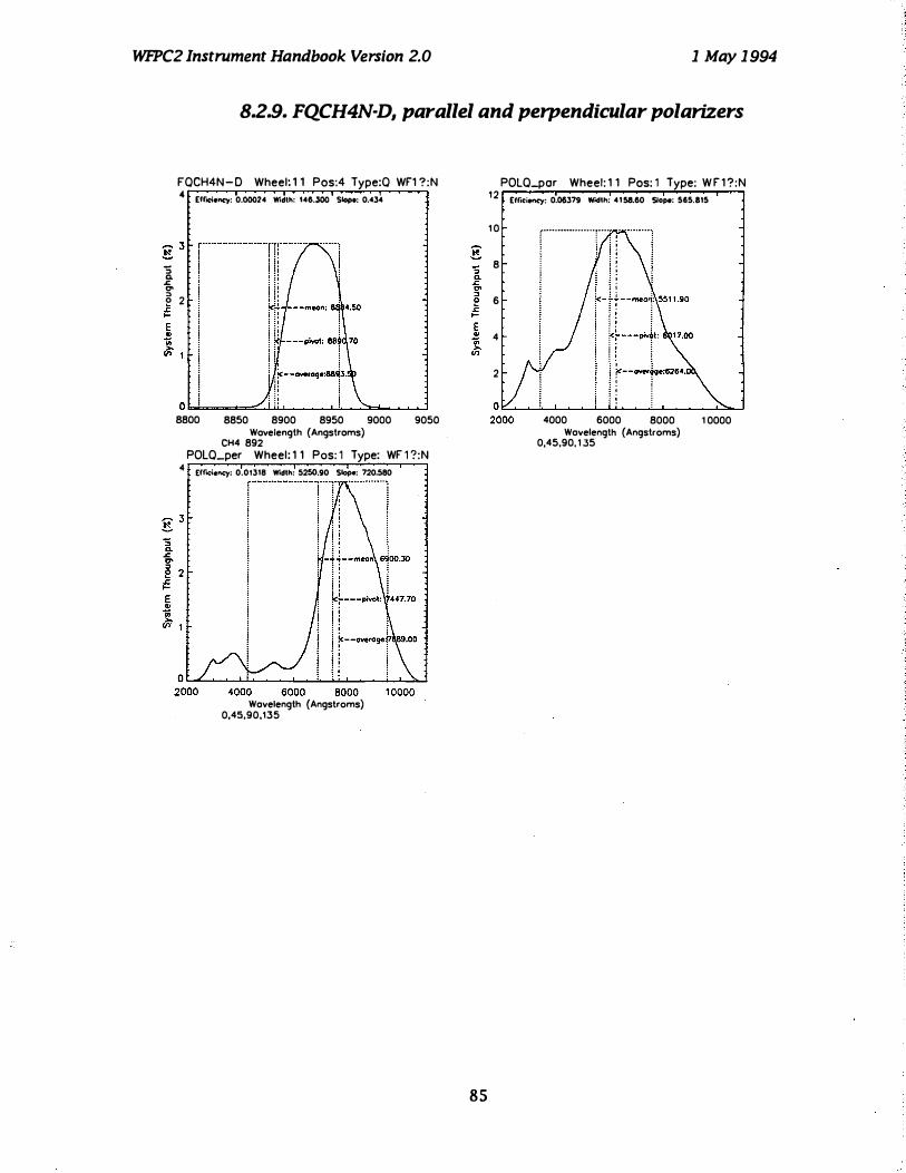
WfPC2 Instrument Handbook Version 2.0 1 May 1 994
8.2.9. FQCH4N-D, parallel and perpendicular polarizers
"S Co .J:. .,. ::>
rOCH4N - D Wheel: 1 1 Pas:4 Type:O WF1 ?:N " ElrlCi.n<y: 0.00024 Wodth: 146.300 Slope: 0.434
o 2 �
O �==������������
8800 8850 8900 8950 9000 9050 Wavelength (Angstroms)
CH4 892 POLO_per Wheel: 1 1 Pas: 1 Type: WF 1 ?:N
4 ElrlCi.n<y: 0.01318 Wodth: 5250.90 Slope: 720.580
Wovelength (Angstroms) 0,45,90,135
85
POLO-por Wheel: 1 1 Pas: 1 Type: W F 1 ?:N 12 E/focioney: 0.06379 w"odth: 41 58.60 Slope: 565.815
1 0
8
6
4
2
,. .................. .. , .... , .. ! � I ' I 4000 6000 8000
Wovelength (Angstroms) 0,45,90, 1 35
1 0000

WfPC2 Instrument Handbook Version 2.0 1 May 1994
8.3. NORMAUZED PASSBANDS INCLUDING THE SYSTEM REsPONSE
II ..
: '�n :::�
sy,
�>� � � 1 0
�00
----�2
�00
�0-----
30�
0-
0----
4-
0·
0-0
----5-
0�0
-0
----6-0
�00
-----7
�00
-0--�-
80�
0-
0�--
9-
0·
0-
0--�
1=0
�00
-0�--
1�1 000
Z Wovelength (Angstroms) II .. � 1 00 � __ ����r-�----��
W-id-e
__ F-il�t-e�rs
�+�
S�y_s_t
_e�m--R�e-s�p_o_n_s_e� ______ �----�----�
:c 80 / l""'\ V ................... . � �g j / \ \ ::::::::::::::.: 1 28 ������ __ �'-__ � __ ��!.! __ Lf_i __
�_\,_,_ .. � ... � .. l�\ ____ ::'_.::_:::�:::_::_:::_:::_: ��� ____
� ____ �
(; 1 000 2000 3000 4000 5000 6000 7000 8000 9000 1 0000 1 1 000 Z Wovelength (Angstroms) .. .. � 1 00 � ____ -r ____ �� ____
W_iTd_e_U_B_V __ R
�l
rF_il_te_r_s
�+
�S�y�
s�te_m
��R
_e�s�p_o�n_s_e
____ � ______ � ____ �
; � /'<ir' ("\t-�'---,,� ��?�?� "I! � 28 � ____ ��� __ � __ �� ____ �!�_i� __ �/�' ______ ��\ ____ �
'�\ � __ �\ ______ � ____ � E (; 1 000 2000 3000 4000 5000 6000 7000 8000 9000
Z Wovelength (Angstroms) 1 0000 1 1 000
.. .. � 1 00 r--____ �----__ ��_W_F-
PT
C�
2�
U-B-V-
R�
I�F
-il-te�r
�s�
+�
s�y�s�te
�m,-�
R-e-s�p�o_n-s-e----�----�----__, :c 80 ! \ // " / - " .� ... ,
'---", ;' '.4 ,'" ..... I • ..... .... � 60 . J.-, " \{ ' ; "--g 40 .,1 /\ ! \" ! \ ........ -. __ ._ .. 1 28 � ____ � ______ L-__ �� __ �!�\� ______ �: ___ ,,,�_�_ �1 ___ ;�., __ � ______ �-_'--'� __ � ____ � (; 1 000 2000 3000 4000 5000 6000 7000 8000 9000 1 0000 1 1 000
Z Wovelength (Angstroms) .. .. � 1 00
�r-__ -r ______ �-----M�
e-d_iu-m
�F�
i-lt-e�
rs __ +�S�y�s-t-e_m�R-e_s�p_o_n_s�e ______ � ______ ���, ____ _, ! �g n ... ,n,.,. / \ �:��:��:��:.:�:.: J���l { \\ � 28 \ 1 \ i \. i \,
E ���==--------����----�----�----�----�--���� (; 1 000 2000 3000 4000 5000 6000 7000 8000 9000 1 0000 1 1 000
Z Wavelength (Angstroms) .. .. � 1 00 r--____ �----__ ����
N-a�
rrr
O-wT7
F�
i-lt-e-rs--
+�
S�y�
s-t�e
�m
�R-e_s�p_o_n_s�e ______ � __ � __ r-____ _, i ij��---.I�����I_���·��� ............... liii� ............... 1 11 ............... ! .............. 1 ............... �; 11:.0.....0..-1 ������������-...........��� li�i�� -........-.....11 ...............
(; 1 000 2000 3000 4000 5000 6000 7000 8000 Z Wavelength (Angstroms) ..
9000 1 0000 1 1 000
.. � 1 00 r-____ -r ______ �--�nTQ--u_O-d-F
-i�lt-e-rs
�+--S�y�s
rt-e-m--R�e-s
�p_o_n_s_e� ____ �� ____ � ____ --, i ��_��_�������_��_��_I�I�I_�_��i=[�\ ___ ��I ___ �f�1 ___ ��� ___ �� ______ � ___ � (; 1 000 2000 3000 4000 5000 6000 7000 8000
Z Wavelength (Angstroms)
86
9000 1 0000 1 1 000
, b